HYDROLOGICAL PROCESSESHydrol. Process. 26, 2663–2671 (2012)Published online 6 July 2012 in Wiley Online Library(wileyonlinelibrary.com) DOI: 10.1002/hyp.9414

Areal differentiation of snow accumulation and melt betweenpeatland types in the James Bay Lowland

Peter Whittington,1* Scott Ketcheson,1 Jonathan Price,1 Murray Richardson2 and Antonio Di Febo31 University of Waterloo, 200 University Ave., Waterloo, ON, N2L 3G1, Canada2 Carleton University, 1125 Colonel By Drive, Ottawa, ON, K1S 5B6, Canada

3 AMEC, 160 Traders Blvd. E., Suite 110, Mississauga, ON, Canada

*CMaE-m

Co

Abstract:

Snow accumulation and melt between various peatland types in the James Bay Lowlands is poorly understood despite being asignificant source of fresh water to the saline James Bay. Many topographical factors that control snow accumulation and melt(e.g. slope, aspect) are not relevant in the James Bay Lowlands because of the extremely low relief. Thus, vegetationcharacteristics (e.g. winter leaf area index, tree density), which are strongly linked to peatland type, may dictate spatial patterns ofsnow accumulation and melt across the landscape. A 1.5-km long transect that bisected five peatland types representative of thelocal area was used to determine average snow depth, density and water equivalence for each of the landscape units. The peatlandtypes were classified, in part, because of the density of treed vegetation and were named open bog, open shrub fen, low-densitytreed fen, medium density treed bog and high-density treed fen. Those with medium or high-density treed vegetationaccumulated significantly more snow than those with low or open densities. Snow density, however, showed no correlation withlandscape unit, and snowmelt proceeded at similar rates between all landscape units because of the relatively open canopy typicalof this environment. A randomization test showed that the areally weighted basin average snow depth estimates varied by lessthan 10 cm as a result of the small but statistically significant differences in snow accumulation among landscape units. Thesedifferences are therefore relatively unimportant for accurately quantifying basin-wide snow depth in this landscape. Copyright ©2012 John Wiley & Sons, Ltd.

KEY WORDS peatlands; James Bay Lowlands; snow accumulation; snow melt; landscape units; vegetation density

Received 22 July 2011; Accepted 9 May 2012

INTRODUCTION

The James Bay Lowlands (JBL) represent a significantcontribution of the fresh water runoff to the saline JamesBay (Rouse et al., 1992), yet there is a dearth ofinformation on how different types of wetlands behavehydrologically in terms of snow accumulation and melt.Determining the average snow depth, density and waterequivalent for large basins can be critical for an accurateunderstanding of the hydrological processes (e.g. runoff)in these basins (Pietroniro et al., 1996; Hamlin et al.,1998; Woo, 1998; Pomeroy et al., 2002), yet doing so canbe expensive and labour intensive. However, landscapeunits within the same climatic region tend to accumulatesnow with repeatable patterns (Steppuhn and Dyck, 1974;Woo and Marsh, 1978), and thus targeted surveying ineasily identifiable landscape units can improve our regionalgeneralizations from a few measurements (Adams andRoulet, 1982) in targeted terrain types (Woo and Marsh,1978) versus a simple random sample (Elder et al., 1991).At the regional (Steppuhn and Dyck, 1974) or

macroscale (Pomeroy et al., 2002) (10–1000 km) snowaccumulation is controlled by latitude, elevation,orographic influences, atmospheric circulation and large

orrespondence to: Peter Whittington, Geography and Environmentalnagement, University of Waterloo, Waterloo, Canada.ail: whittington.pete@gmail.com

pyright © 2012 John Wiley & Sons, Ltd.

water bodies; at the local or mesoscale (100–1000m), itcan be controlled by terrain variables such as elevation,slope and aspect and vegetation variables such asvegetation type, canopy and tree density; and at themicroscale (10–100m) by interception, surface roughnessand redistribution along airflow patterns. Despite differ-ences in snow accumulation at the microscale, Pomeroyand Gray (1995) note that snow accumulation patterns arestill evident at the stand (meso) scale. These accumulationpatterns typically vary with the effective winter leaf areaindex (LAI; total horizontal area of stems, needles andleaves per unit area of ground) (Pomeroy et al., 2002)and the impact of wind redistribution of snow (Bensonand Sturm, 1993), both of which should be affected bydifferences in the relative tree density between differentlandscape units in the JBL.Snow interception in forested canopies is impacted in

part by the leaf area and tree species (Hedstrom andPomeroy, 1998), and in combination with sublimation,losses directly from the canopy can greatly reduce snowaccumulation in forested sites (Koivusalo and Kokkonen,2002). In areas where the LAI is low, snow accumulationpatterns are similar to those in open areas (Pomeroy et al.,2002). Further, wind-blown snow from adjacent openareas will accumulate in stands of more dense vegetationwhere surface wind speeds are reduced (Benson andSturm, 1993). The JBL is dominated by low LAIlandscape units (e.g. sparse trees in bogs) that have yet

2664 P. WHITTINGTON ET AL.

to be suitably characterized but will likely result in muchsubtler differences in snow accumulation patterns com-pared with forested watersheds with higher average LAIand also higher spatial variability in LAIRelatively little research on snow accumulation and

melt processes has been conducted in low relief andsparsely vegetated landscapes typical of Canada’snorthern lowland regions. Adams and Roulet (1982)studied snow accumulation in a small sub-arctic drainagebasin and found that average snow depth was greatest inareas with the closest spacing of trees (e.g. 146 cm with2–6m spacing and 126 cm with 7–12m spacing) andshallowest in open tundra environments (e.g. 77 cm withshrub covered tundra). Sturm et al. (2001) found that thedeepest snow packs were found in areas with the tallest,densest shrubs in a tundra site in arctic Alaska. Additionalresearch is required to accurately characterize spatialvariability of snow accumulation in JBL sub-arcticlowland environment.The rate of snowmelt at the microscale and macroscale

is controlled and also strongly influenced by thevegetation canopy LAI, hence tree density, and its effecton the energy available for snow ablation (Boon, 2009).A forest canopy will reduce the net radiation andturbulent transfer contributions to snow ablation. Similarto accumulation processes mentioned earlier, the rela-tively open canopies in the JBL may not be notablydifferent than open areas resulting in similar snow meltrates across landscape units.Many studies have used the landscape unit approach in

their snow studies; however, these have largely been usedin the Western boreal forest (e.g. Pomeroy et al., 2002),Southern Ontario forest (Adams, 1976), Sierra Nevadaalpine (Elder et al., 1991), disturbed forest (Boon, 2011)and sub-Arctic (Adams and Roulet, 1982) and high-Arctic (Woo and Marsh, 1978; Woo and Young, 1997;Woo, 1998) systems. Few studies have employed the‘landscape unit’ approach in wetland dominated basins,especially in the JBL where more than 60% of thelandscape is covered by bogs and fens (Riley, 2011).Many of the terrain factors that can affect snowaccumulation at the mesoscale are irrelevant in extremelylow relief areas such as the JBL. Vegetation factors,however, vary with peatland type and are likely toinfluence snow accumulation and ablation patterns.Different peatland types are, in part, a function ofvegetation structure, and unambiguously classifying themis difficult (Di Febo, 2011). While the Canadian WetlandClassification System (NWWG, 1997) categorizeswetlands with a three-level hierarchical system on thebasis of (1) class (e.g. bog or fen), (2) form (e.g. peatplateau bog or channel fen) and (3) type (e.g. treed bog orgraminoid fen), these hierarchical structures, especiallyform, are often difficult to identify. Riley (2011) offers analternative system that ignores form and focuses mostlyon class and type, where type is predominantly vegetationbased. Therefore, using Riley’s (2011) classificationscheme would conveniently divide the landscape intorelatively homogenous ‘landscape units’.

Copyright © 2012 John Wiley & Sons, Ltd.

Considering the limited understanding of snowdynamics between and within different ‘landscape units’in peatland dominated basins, the objective of this paperis to determine the snow pack and melt regimecharacteristics of various peatland types in the JBL.

STUDY SITE

The study site is located 500 km north–north–west ofTimmins, Ontario, and 90 km west of Attawapiskat,Ontario, in the Hudson–JBL (lat. 52.8349, long.�83.9290). The study area comprises part of the NorthGranny Creek (NGC) watershed, which is a tributaryof the Nayshkootayaow River and subsequently theAttawapiskat River (Figure 1). NGC splits into twodistinct channels that we have labelled south-NGC(SNGC) and north-NGC (NNGC).The snow survey transect was 1.5-km long and

bisected five different peatland types common to the area(Figure 1). The start of the transect was a medium densitytreed lichen-rich bog, which led into areas of low-densitytreed fen and high-density treed fens in the riparian areasnear the streams. The bog that separates SNGC andNNGC is similar to that at the southern end of thetransect. At the north end of the transect is an open shrubfen water track classified as open shrub fen. Lastly, thereis an open, lichen-rich low shrub bog at the northernmostend. Table I provides a key to the nomenclature(including transect locations).The two closest stations with long-term meteorological

records were Lansdowne House (inland 300 km west–south–west) and Moosonee (near the coast, 250 kmsouth–east). The average annual January and Julytemperatures for Lansdowne House are �22.3 and17.2 �C, respectively, and for Moosonee are �20.7 and15.4 �C, respectively (Environment Canada, 2008).Annual precipitation for Lansdowne House is 700mmwith ~35% falling as snow; for Moosonee, precipitation is682mm with ~31% falling as snow.The study site is located at the De Beers Victor Mine,

and therefore the possibility of dust enhanced melt (fromblasting in the open pit) must be addressed (Drake, 1981).Drake and Moore (1980) studied dust loading around amine in Schefferville, Quebec, and noted that prevailingwinds were a large control on dust fall and that within adistance of 1 km cross-wind from the disturbed area, dustfall returns to a ‘. . .presumably normal background level’.The normal background values by Drake and Moore(1980) are reported as 2 g/m2 over the winter season(~6months). The study area at the Victor Mine is locatedseveral (3–4) kilometres directly upwind of the mine, andthus dust fall is likely not an issue. In addition, as part ofDe Beers’ monitoring requirements, dust fall is collectedat four orthogonal locations around the mine. At thelocation nearest the transect, dust falls for 2008, 2009 and2010 for May were 0.8, 1.8 and 1.2 g/m2/30 days(Steinback (De Beers Canada, Victor Diamond Mine),pers. comm.; 2011 data were not ready for release, but

Hydrol. Process. 26, 2663–2671 (2012)

Medium bog

Low density fen

High density fen

Medium bog

High density fen

Openshrub fen

Openbog

Medium bog

Low density fen

High density fen

Medium bog

High density fen

Openshrub fen

Openbog

a)

c)b)

Figure 1. Site map. (a) Location of study area within Ontario. (b) IKONOS image showing part of the NGC watershed divided into the NNGC and SNGCsubwatersheds (white lines) and the streams (black lines). The De Beers Victor mine camp is visible in the lower right hand corner; the pit is located ~1kmfurther to the right. The image is approximately 9 km across. (c) IKONOS image of the snow survey transect (solid white line), ablation lines and snow pits (allstars 2009, grey stars 2011) and landscape types along the transect. The transect is 1500m long. Note: Some high vegetation density fen sites do exist in the low-

density fen areas but have been omitted in Figure 1 and Table I for simplification. They were classified correctly for all analyses

Table I. Landscape classification class and type

Tree properties

Distance along transect (m) Classification (Riley, 2011) Official This paper Height (m) Distance (m) % treed

0 to 145; 615 to 810 Medium density treed lichen-rich bog T(md)lrB Medium bog 3.3 16 50145 to 580 Open treed or low-density treed fen T5F-T(ld)F Low-density fen 3.9 17 18580 to 615; 810 to 866 High-density treed fen T(hd)F High-density fen 3.9 4 63886 to 1200 Open shrub fen OsF Open shrub fen 3.0 29 61200 to 1500 Open, lichen-rich low shrub bog OlrlsB Open bog 3.7 35 12

The superscript T5 is a quantification of how open the area is, e.g. <5% tree cover. The letters can be deduced from the classification column. Treedistance was determined from the manual tree density survey. Height was determined as the average of non-zero returns from the canopy height model.% treed was calculated as the number of non-zero returns for that landscape type/total returns (zero and non-zero) for that landscape type� 100.

2665AREAL DIFFERENTIATION OF SNOW ACCUMULATION AND MELT IN THE JBL

as the pit continues to get deeper, the risk of dustcontamination diminishes), which, although slightly higher,are in-line with those reported by Drake and Moore (1980).

METHODS

Meteorological

A weather station was erected ~1 km south of theVictor Mine in March 2000; this weather station wasdecommissioned when a new weather station was erected~2 km north of the Victor Mine near the study area inApril 2008. Both weather stations measured precipitation,temperature, relative humidity, net radiation, wind speedand direction.

Snow surveys and ablation lines

Snow surveys were conducted every 4–5 days fromApril to May in 2009 and 2011 along the research

Copyright © 2012 John Wiley & Sons, Ltd.

transect. In 2010, there was an abnormally low snowfalland early melt and is not considered in this paper. Depthmeasurements using ametal ruler were taken every 15 paces(~10m)with depth and snowwater equivalent (SWE) every30 paces using an ESC-30 (Eastern Snow Conference)plastic snow tube (1.2m by 0.07m i.d.) and hanging massscale. SWE was calculated on the basis of the mass of thesnow in the tube and water density of 1 g/cm3; snow densitywas calculated using the volume (depth of the sample andtube dimension). At each SWE measurement location, aGPS reading (�4m) was taken to locate the landscape typesampled (a separate ground truthing survey for landscapeclassification was completed in November 2009). Tomeasure the rate of snowmelt, measurements of the changein snow surface elevationweremade at 0.5m intervals along6.5 to 10.5m ablation wires. In 2009 (all stars, Figure 1),they were erected in medium bog (x2), low-density fen (x2)and open shrub fen (1) (Figure 1) and, in 2011 (grey starsonly, Figure 1), in medium bog (1) and low-density treed

Hydrol. Process. 26, 2663–2671 (2012)

Win

d sp

eed

(m/s

)

2666 P. WHITTINGTON ET AL.

fen (1). Snow pits were used to measure density andtemperature profiles in the area near each ablation line inboth years; however, they were only completed once in2011. Density samples were taken using a fixed volumecutter (6� 3� 5.5 cm=99 cm3) centred at every 5 cm forthe entire snow pit depth. Ablation lines and snow pits weremeasured when they were reached along the snow surveytransect. Different snow pits in roughly the same area(within 5m) were used each time.

Tree canopy properties

Starting at the southern end of the transect, the distanceand the diameter at breast height (DBH) was measured forthe closest tree in each quarter [following the point-quarter method (Cottam and Curtis, 1956)] at a pointevery 50m along the transect. Because of the stuntedgrowth of trees in the JBL, the definition of tree wasextended to those with a DBH of 6 cm rather than 10 cm.Where canopy cover was very open (e.g. north end of thetransect) and trees would be double counted (i.e. the sametree would be the closest for the subsequent quarter), thespacing was increased or the survey stopped.To create the canopy height model, a 5-m resolution

digital surface model (DSM) was first interpolated usingthe maximum elevation of all LiDAR returns using a 5 by5m moving window that followed the snow surveytransect. The ground surface elevation was subtractedfrom this DSM using the 5-m resolution bare earth digitalelevation model (DEM). Areas with no classifiedvegetation returns were assigned a height of 0m.

Landscape classification

The watershed boundaries and landscape compositionare based on classification of LiDAR and IKONOSremote sensing imagery (Di Febo, 2011). Briefly, amaximum likelihood classification was conducted on theIKONOS red, green, blue and near-infrared bands as wellas several topographic derivatives computed from a 2.5-mresolution LiDAR derived DEM that were shown toimprove the classification accuracy. The final cross-validated accuracy of the classification (using separatetraining and validation classes and excluding water,which is relatively easy to discriminate) was approxi-mately 80%.

Tem

pera

ture

(°C

)

Figure 2. Meteorological variables for the 2009 and 2011 melt seasons

RESULTS

The average April temperature (when the majority of themelt occurs) based on the 8-year record located on site(2000–2007) fell between those at Lansdowne House andMoosonee, suggesting that those stations could be usedfor the long-term average. The average daily temperaturesfor April 2009 and 2011 and the 30-year LansdowneHouse and Moosonee averages were, �2.9, �2.2, �2.4and �1.6 �C, respectively, making 2009 slightly coolerthan average and 2011 average. The first half of April2009 averaged �6 �C, whereas for 2011, it was �3 �C, in

Copyright © 2012 John Wiley & Sons, Ltd.

part because of a warm period (average daily tempera-tures >0) for 4 out of 5 days (and the <0 day dailytemperature was only �1.8 �C) from 8 April to 13 April2011; the second half of April was similar for both years(Figure 2). In 2009, a 5-day warm period occurred from13 April to 18 April, with 16 April 2009 having a dailyaverage and max temperature of 7.4 and 15.3 �C,respectively. Wind speeds were higher for the start ofmelt in 2009 but were similar between years after ~18April 18. For 2009 and 2011, snow accumulation at theend of March (i.e. near the start of melt) was 133% and71%, respectively, of the normal values reported atLansdowne House (inland station), although snow melt in2011 had started prior to our arrival.In 2009, snowmelt started on 9 April and continued

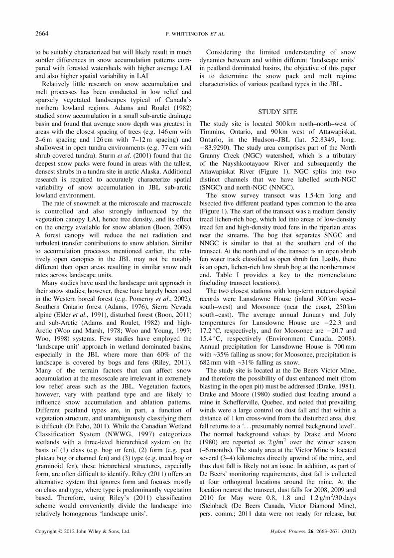
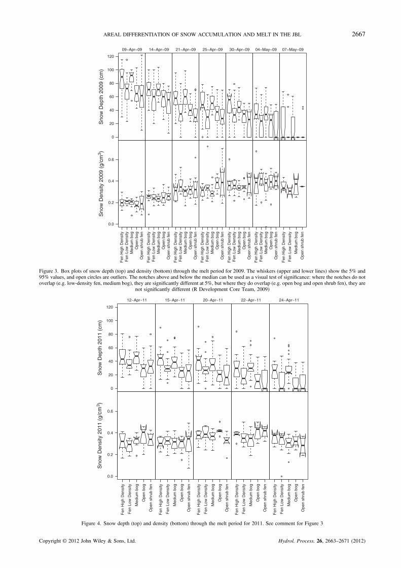
until ~7 May. Average snow depth across the site was75 cm at the onset of melt, ranging from 63 cm in theopen shrub fen to 90 cm in the medium bog (Figure 3). In2011, snow melt had started before we arrived on site andsome ripening and settling of the snow pack hadoccurred; however, very few bare patches were present(the tops of a few hummocks at the northern end of thetransect were visible). Average snow depth upon arrivalin 2011 was 39 cm, ranging from 27 cm in the open bogto 47 cm in the high-density fen (Figure 4). Thecompletion of melt was not well documented in 2011because of limited field personnel but the site becamesnow free ~28 April. For both years, the medium bog and

Hydrol. Process. 26, 2663–2671 (2012)

0

20

40

60

80

100

120

09−Apr−09

Sno

w D

epth

200

9 (c

m)

14−Apr−09 21−Apr−09 25−Apr−09 30−Apr−09 04−May−09 07−May−09

Fen

Hig

h D

ensi

tyF

en L

ow D

ensi

tyM

ediu

m b

ogO

pen

bog

Ope

n sh

rub

fen

0.0

0.2

0.4

0.6

Fen

Hig

h D

ensi

tyF

en L

ow D

ensi

tyM

ediu

m b

ogO

pen

bog

Ope

n sh

rub

fen

Fen

Hig

h D

ensi

tyF

en L

ow D

ensi

tyM

ediu

m b

ogO

pen

bog

Ope

n sh

rub

fen

Fen

Hig

h D

ensi

tyF

en L

ow D

ensi

tyM

ediu

m b

ogO

pen

bog

Ope

n sh

rub

fen

Fen

Hig

h D

ensi

tyF

en L

ow D

ensi

tyM

ediu

m b

ogO

pen

bog

Ope

n sh

rub

fen

Fen

Hig

h D

ensi

tyF

en L

ow D

ensi

tyM

ediu

m b

ogO

pen

bog

Ope

n sh

rub

fen

Fen

Hig

h D

ensi

ty

Fen

Low

Den

sity

Med

ium

bog

Ope

n sh

rub

fen

Sno

w D

ensi

ty 2

009

(g/c

m3 )

Figure 3. Box plots of snow depth (top) and density (bottom) through the melt period for 2009. The whiskers (upper and lower lines) show the 5% and95% values, and open circles are outliers. The notches above and below the median can be used as a visual test of significance: where the notches do notoverlap (e.g. low-density fen, medium bog), they are significantly different at 5%, but where they do overlap (e.g. open bog and open shrub fen), they are

not significantly different (R Development Core Team, 2009)

0

20

40

60

80

100

120

12−Apr−11

Sno

w D

epth

201

1 (c

m)

15−Apr−11 20−Apr−11 22−Apr−11 24−Apr−11

Fen

Hig

h D

ensi

ty

Fen

Low

Den

sity

Med

ium

bog

Ope

n bo

g

Ope

n sh

rub

fen

0.0

0.2

0.4

0.6

Fen

Hig

h D

ensi

ty

Fen

Low

Den

sity

Med

ium

bog

Ope

n bo

g

Ope

n sh

rub

fen

Fen

Hig

h D

ensi

ty

Fen

Low

Den

sity

Med

ium

bog

Ope

n bo

g

Ope

n sh

rub

fen

Fen

Hig

h D

ensi

ty

Fen

Low

Den

sity

Med

ium

bog

Ope

n bo

g

Ope

n sh

rub

fen

Fen

Hig

h D

ensi

ty

Fen

Low

Den

sity

Med

ium

bog

Ope

n bo

g

Ope

n sh

rub

fen

Sno

w D

ensi

ty 2

011

(g/c

m3 )

Figure 4. Snow depth (top) and density (bottom) through the melt period for 2011. See comment for Figure 3

2667AREAL DIFFERENTIATION OF SNOW ACCUMULATION AND MELT IN THE JBL

Copyright © 2012 John Wiley & Sons, Ltd. Hydrol. Process. 26, 2663–2671 (2012)

Table II. p-values of Wilcoxon rank sum difference of means test for snow density (below diagonal) and snow depth (above diagonal)at onset of snowmelt (2009/2011)

Fen high density Fen low density Medium bog Open bog Open shrub fen

Fen high density — ≤0.01/≤0.01 0.95/0.90 ≤0.0001/≤0.0001 ≤0.001/0.013Fen low density 0.90/0.43 — ≤0.0001/≤0.0001 0.45/0.24 0.29/0.32Medium bog 0.73/0.79 0.76/≤0.05 — ≤0.0001/≤0.01 ≤0.0001/≤0.001Open bog 0.29/0.22 0.10/≤0.05 0.20/0.20 — 0.48/0.03Open shrub fen 0.86/0.53 0.87/0.10 0.91/0.71 0.53/0.23 —

Bold entries significant at 95% or better.

0

1

2

3

4

5

6

7

8

20-Apr-09 24-Apr-09 28-Apr-09 2-May-09 6-May-09 10-May-09Su

rfac

e lo

wer

ing

(cm

/day

)

Medium bog 1 Low density fen 1

Low density fen 2 Medium bog 2

Open shrub fen

0

2

4

6

8

10

12

April 14, 2011 April 17, 2011 April 20, 2011 April 23, 2011 April 26, 2011

Su

rfac

e lo

wer

ing

(cm

/day

)

Medium bog 1

Low density fen 2

0.0

0.5

1.0

1.5

2.0

2.5

20-Apr-09 22-Apr-09 24-Apr-09 26-Apr-09 28-Apr-09

Mel

t (c

m/d

ay)

Medium bog 1 Low density fen 1

Low density fen 2 Medium bog 2

Open shrub fen

a)

b)

c)

Figure 5. Snow surface lowering determined from ablation lines for 2009(a) and 2011 (b) and the corresponding melt rates for 2009 (c). Snow pits

were not completed on the last day

2668 P. WHITTINGTON ET AL.

high-density fen were above average in snow accumula-tion and were statistically significantly different than theopen shrub fen, low-density fen and open bog, whichwere below average (Table II).At the onset of melt in 2009, snow density ranged from

0.17 to 0.20 g/cm3 in the open bog and low-density fen,respectively, but offered no real trend with landscape type(Figure 4). Snow water equivalence ranged from 12 cm inthe open shrub fen to 18 cm in the medium bog. The siteremained completely snow covered until 13 April andbecame functionally snow free ~7 May (some small,isolated drifts in heavily treed areas remained) (Figure 3).In 2011, snow density ranged from 0.28 g/cm3 in the low-density fen to 0.36 g/cm3 in the open bog on the first dayof measurement (Figure 4). Again, no real trend withlandscape type was observed. SWE was highest in themedium bog at 16 cm on the first day of measurementsand was lowest in the low-density fen with 11 cm. In bothyears, the medium bog had the highest SWE followed byhigh-density fen. Open bog was the second lowest inboth years.The rate of snow surface lowering beneath the ablation

lines in 2009 and 2011 were very similar betweenlandscape types for the same period for both years andranged between 0.5 and 10 cm/day (Figure 5a and b). Thelarge increase in the second medium bog location was dueto some small patches of relatively deep snow remainingthat melted to nothing very quickly. For 2009, thesecorresponded to melt rates of between 2.3 and 0.24 cm/day(Figure 5c) and again were similar between all landscapetypes. The fewer points are a result of no snow pits beingconducted on the last measurement days because of a veryshallow snow pack.Temperature profiles (not shown) in the snow pits in

2009 showed the snow profile in all five of the pitsbecoming isothermal and ripe (~0 �C) around 21 Aprilshortly after the warm period noted previously (Figure 2).In 2011, the first (and only) snow pits (April 12) showedan already isothermal and ripe snow pack, again,corresponding with the end of the warm period (Figure 2).The average distance to a tree (which is an inverse

surrogate for tree density) is being used in this paperinstead of tree density as it removes the need for dividingby an arbitrary area (e.g. hectares) to convert distance to adensity. Snow depth at the onset of melt (or first surveyfor 2011) was inversely correlated to average distance totree (Table I, Figure 6). The open bog point was

Copyright © 2012 John Wiley & Sons, Ltd.

artificially placed at 35-m distance as the tree densitysurvey was stopped because of very low tree density(35m was the furthest distance recorded in the open shrubfen before the survey was terminated). The R2 valuesexcluding the open bog point for 2009 and 2011 are 0.52and 0.56, respectively. The open fen and open bog had6% and 12% tree coverage on the basis of the canopymodel created by the LiDAR, compared with 50% and63% coverage for the medium bog and high-density fenlocations, respectively (Table I). Shrub heights were notpart of the original tree survey; however, personalobservations show that in the medium bogs, shrubs were~<60 cm tall and spaced similarly to the trees. In the openfen and open bog, shrubs were much more prevalent thantrees however less frequent that in the medium boglocations and were smaller (~<45 cm).

Hydrol. Process. 26, 2663–2671 (2012)

0

10

20

30

40

50

60

70

80

90

100

0 5 10 15 20 25 30 35 40

Sno

w d

epth

(cm

)

Distance to tree(m)

High density fen Medium bog

Low density fen

Open fen Open bog

High density fenMedium bog

Low density fenOpen fen

Open bog

2009R2 = 0.5873

2011R2 = 0.8049

Figure 6. Average distance to tree versus snow depth for the different landscape types for 2009 (dark) and 2011 (white) initial snow survey. Recall treebeing defined at a DBH> 6 cm

Table III. % area for each of the landscape units of the NorthGranny Creek basin and an example of the randomization for

9 April 2009

Snow depths 9 April 2009

Areally weighed

Landscape Unit Area (%) Survey Correct Max Min

High-density fen 8 85.9 85.9 62.8 90.5Open bog 17 65.4 65.4 65.4 85.9Open shrub fen 19 62.8 62.8 67.7 67.7Medium bog 26 90.5 90.5 85.9 65.4Low-density fen 30 67.7 67.7 90.5 62.8

Average 74.5 73.7 78.6 70.4

For example, the high-density fen occupied 8% of the area and contained85.9 cm of snow on the basis of the field survey and therefore contributes0.08� 85.9 cm= 6.9 cm of the 73.7-cm basin average for the ‘correct’areally weighed allocation column.

0.0

10.0

20.0

30.0

40.0

50.0

60.0

70.0

80.0

90.0

April 9, 2009 April 14, 2009 April 19, 2009 April 24, 2009 April 29, 2009 May 4, 2009

Sno

w d

epth

(cm

)

Figure 7. Randomized areally weighted average snow depths for the NGCbasin. Whiskers in these box plots represent min and max

2669AREAL DIFFERENTIATION OF SNOW ACCUMULATION AND MELT IN THE JBL

DISCUSSION

Classification of any landscape into ‘landscape units’ isdifficult, especially low relief environments such as theJBL. Riley’s (2011) system offers more flexibility overthe NWWG (1997) as many of the types are scaledependant on the density of treed vegetation. Snow depthin this peatland complex varied by site (Figures 3 and 4)and was statistically significant between those with higherdensity and those with lower density (Table II). Forinstance, low-density and high-density fen were different;however, low-density fen and open bog or open shrub fenwere not. This is also supported by the strong correlationbetween snow depth and tree distance (Figure 6). Siteswith high or medium tree densities had snow depth abovethe overall average, and those with low tree densities werebelow; this trend was consistent for both years’ data.Snow density, however, was similar among landscapetypes, and almost none were significantly different.Melt rates were similar between landscape types, and

most proceeded at very similar rates (Figure 5c),regardless of tree density. While the snow is deeper inareas with denser tree cover, shading by the canopy ofthese stunted, relatively well-spaced trees is minimal, andat almost all points along the transect, there is always aclear view of the sky. Reifsnyder and Lull (1965) showedthat in forested environments (red pine), reducing canopycover from 1.5m average distance to tree to 7.7mincreased light intensity from 15 to 60%. As the treedistance is much larger in our study area (16 to >35m)and the stunted black spruce typical of the JBL wouldhave an already more open canopy than red pine, it is notsurprising that melt rates proceeded similarly amonglandscape types. Exceptions to this are the very denseforested areas near the streams (average distance to tree of<4m), but these represent a small proportion of the area[about 3% (Di Febo 2011)]. Therefore, the denser treecover generally encourages snow deposition, likely due tolower wind speeds (Benson and Sturm, 1993; Ketchesonet al., 2012), but is insufficient to markedly reduce theradiation budget and thus the rate of melt. While we donot have meteorological instruments in the forestedsections to quantify the wind speed differences, fieldobservations support lower wind speeds in the treed areas

Copyright © 2012 John Wiley & Sons, Ltd.

compared with the open fen and bog. Therefore, theduration of the snowmelt period in the JBL is ultimatelydependant on how much snow was present at the start ofthe melt and the radiation balance.Our results indicate small but statistically different

snow depths between the majority of the landscape unitsat this JBL study site. In order to test whether thesedifferences were hydrologically important at the scale ofthe entire drainage basin, a simple reallocation experimentwas conducted. On the basis of the analysis of Di Febo(2011), we were able to relate our landscape units to Di

Hydrol. Process. 26, 2663–2671 (2012)

2670 P. WHITTINGTON ET AL.

Febo’s (2011) to areally weight the snow depths for theentire basin for the snow melt period. These areallyweighted basin average snow depth values were alwayswithin 0.8 cm (Table III) of the field snow survey average,suggesting that the snow survey chosen was representa-tive of the basin as a whole (Table III). To test theimportance of the differences between landscape units,observed snow depths were re-assigned to different landcover types iteratively until all possible permutations ofland cover type/snow depth observations were satisfied.The basin average snow depth was re-calculated eachiteration and recorded. There are five landscape units, andtherefore, there are 120 (5! = 5� 4� 3� 2� 1 = 120)ways (permutations) of reallocating the depths to thelandscape unit areas. Table III shows an example for thefirst day of snow surveys in 2009. The snow surveyaverage was 74.5 cm at the onset of melt, which comparedwell with the average of the ‘correct’ order of areallyweighting the depths of 73.7 cm. The maximum (maxcolumn, Table III) would be one outcome (of the 120)where the depths arranged themselves ascending withascending area (i.e. the shallowest snow depths with thesmallest areas), whereas the minimum (min column,Table III) would occur when they were arranged inreverse. For example, the 62.8-cm average depth for openshrub fen was applied to the area for high-density fen(max) and then to low-density fen (min) (Table III). Theoutcomes of the other 117 (min, max, and correct) casesare summarized using box plots (Figure 7). The range(max–min) varied between 5.2 and 8.3 cm, with anaverage range of 6.9 cm. The inter-quartile range (upper–lower quartile) where 50% of the outcomes would occurranged from 2 to 3.6 cm, with an average of 2.8 cm. Giventhe large natural variability of snow depth within alandscape type (Figures 3 and 4), these ranges are wellwithin the expected error of measurement, implying thatwhile landscape types do, generally, have statisticallysignificantly different snow packs than each other, thisdifference is not important to the basin’s averagesnow depth.

CONCLUSION

In this area of the JBL, snow depth is controlled mostlyby land cover type and its associated vegetationcharacteristics, as opposed other landscapes wheretopography, aspect and slope have a much strongerinfluence on snow depth. Despite differences in snowdepth, melt rates were similar across all landscape types,in part because of the relatively open canopy coverthroughout this sparsely vegetated landscape. Because ofthe similar proportions of open bog/fen and low/mediumfen and bog, and small area of high-density fen, changingthe distribution of snowfall by re-allocating it did notsignificantly affect the average basin snow depth. Ourfindings contrast those of many other studies that haveshown that topography and vegetation strongly influencethe spatial pattern of snow accumulation and melt and

Copyright © 2012 John Wiley & Sons, Ltd.

must be specifically addressed as part of any snowsampling strategy designed to estimate basin-wide snowdepth. Here, we found that a simple snow survey thattransects some open and treed areas is sufficient toestimate basin-wide snow depth.

ACKNOWLEDGEMENTS

The authors wish to thank Dave Fox, Chris Cook, TomUlanowski, Melissa Leclair and Emily Perras forassistance in the field. Special thanks must be given tothe Environment Lab at the De Beers Victor mine foreverything they have done for us. Thanks also to the keeneye of one of the reviewers of this paper. Funding wasprovided in part by De Beers Canada and an NSERCCRD grant to J. Price.

REFERENCES

Adams W. 1976. Areal differentiation of snow cover in east centralOntario. Water Resources Research 12(6): 1226–1234.

Adams W, Roulet N. 1982. Areal differentiation of land and lakesnowcover in a small sub-Arctic drainage basin. Nordic Hydrology 13(3):139–156.

Benson CS, Sturm M. 1993. Structure and wind transport of seasonalsnow on the Arctic slope of Alaska. Annals of Glaciology 18:261–267.

Boon S. 2009. Snow ablation energy balance in a dead forest stand.Hydrological Processes 23(18): 2600–2610.

Boon S. 2011. Snow accumulation following forest disturbance.Ecohydrology. DOI: 10.1002/eco.212

Cottam G, Curtis JT. 1956. The use of distance measures inphytosociological sampling. Ecology 37(3): 451–460.

Di Febo A. 2011. On developing an unambiguous peatland classificationusing fusion of IKONOS and LiDAR DEM terrain derivatives. VictorProject, James Bay Lowlands, University of Waterloo, Waterloo.

Drake J. 1981. The effects of surface dust on snowmelt rates. Arctic andAlpine Research 13(2): 219–223.

Drake J, Moore TR. 1980. Snow pH and dust loading at Schefferville,Quebec. Geographica XXIV(3): 286–291.

Elder K, Dozier J, Michaelsen J. 1991. Snow accumulation anddistribution in an alpine watershed. Water Resources Research 27(7):1541–1552.

Environment Canada. 2008. Canadian Climate Normals or Averages1971–2000.

Hamlin L, Pietroniro A, Prowse TD, Soulis E, Kouwen N. 1998.Application of indexed snowmelt algorithms in a northern wetlandregime. Hydrological Processes 12: 1641–1657.

Hedstrom N, Pomeroy J. 1998. Measurements and modelling of snowinterception in the boreal forest. Hydrological Processes 12(10–11):1611–1625.

Ketcheson SJ,Whittington P, Price JS. 2012. The effect of peatland harvestingon snow accumulation, ablation and snow surface energy balance.Hydrological Processes accepted Dec 2011. DOI: 10.1002/hyp.9325

Koivusalo H, Kokkonen T. 2002. Snow processes in a forest clearing andin a coniferous forest. Journal of Hydrology 262(1–4): 145–164.

National Wetlands Working Group. 1997. The Canadian WetlandClassification System, 2nd edn. University of Waterloo, Waterloo,Ontario.

Pietroniro A, Prowse TD, Hamlin L, Kouwen N, Soulis R. 1996.Application of a grouped response unit hydrological model to anorthern wetland region. Hydrological Processes 10(10): 1245–1261.

Pomeroy J, Gray D. 1995. Snowcover accumulation, relocation andmanagement. Bulletin of the International Society of Soil Science88: 2.

Pomeroy JW, Gray DM, Hedstrom NR, Janowicz JR. 2002. Prediction ofseasonal snow accumulation in cold climate forests. HydrologicalProcesses 16: 3543–3558.

R Development Core Team. 2009. R: a language and environment forstatistical computing. R Foundation for Statistical Computing.

Hydrol. Process. 26, 2663–2671 (2012)

2671AREAL DIFFERENTIATION OF SNOW ACCUMULATION AND MELT IN THE JBL

Reifsnyder WE, Lull HW. 1965. Radiant energy in relation to forests.In Service, U.S.D.o.A.F. (ed.). U.S. Government Printing Office:Washington D.C.; 125.

Riley JL. 2011. Wetlands of the Ontario Hudson Bay Lowland: an regionaloverview. Nature Conservancy of Canada, Toronto, Ontario, Canada; 156.

Rouse WR, Woo M, Price JS. 1992. Damming James Bay: I. Potentialimpacts on coastal climate and the water balance. The CanadianGeographer 36(1): 2–7.

Steppuhn H, Dyck G. 1974. Estimating true basin snowcover, advancedconcepts and techniques in the study of snow and ice resources: aninterdisciplinary symposium;[papers]. National Academies.

Copyright © 2012 John Wiley & Sons, Ltd.

Sturm M, McFadden JP, Liston GE, Chapin FS, III, Racine CH, HolmgrenJ. 2001. Snow-shrub interactions in Arctic tundra: a hypothesis withclimate implications. Journal of Climate 14: 336–344.

Woo M. 1998. Arctic snow cover information for hydrologicalinvestigations at various scales. Nordic Hydrology 29(4/5): 245–266.

Woo M, Marsh P. 1978. Analysis of error in the determination of snowstorage for small high Arctic basins. Journal of Applied Meteorology17: 1537–1541.

Woo M, Young KL. 1997. Hydrology of a small drainage basin with polaroasis environment, Fosheim Peninsula, Ellesmere Island, Canada.Permafrost and Periglacial Processes 8: 257–277.

Hydrol. Process. 26, 2663–2671 (2012)