SNOW ACCUMULATION ALGORITHM FOR THE WSR-88D RADAR,

VERSION 1

June 1996

U.S. DEPARTMENT OF THE INTERIOR Bureau of Reclamation

Technical Service Center Water Resources Services

River Systems and Meteorology Group

I REPORT DOCUMENTATION PAGE I OMB No 0704-0188 1 Fonn Approved

I

Pubhc reporting burden for this collection of mfonatlon 1s estimated to average 1 hour per response, ~ncludlng the tlme for revlewmg lnstrunlons. searching exlstlng data sources, gather~ng and malntalnlng the data needed, and completing and revlewlng the collection of lntormat~on Send comments regardmg th~s burden estlmate or any other aspect of th~s coltectlon of ~nformat~on. lnclud~ng suggestions for reducmg thls burden to Washmgton Headquaners Se~ lces . D~rectorate for Informatton Operat~ons and Reports 1215 Jefferson Dav~s H~ghway. Sult 1204. Arlmgton VA 22202-4302. and to the OWlce of Management and Budget, Paperwork Reduction Report (0704-01 88). Wash~ngton DC 20503

1. AGENCY USE ONLY (Leave Blank) 1 2. REPORT DATE 1 3. REPORT TYPE AND DATES COVERED I ~ u n e 1996 I Final

4. TITLE AND SUBTITLE Snow Accumulation Algorithm for the WSR-88D Radar, Version 1 6. AUTHOR(S) Arlin B. Super and Edmond W. Holroyd, 111

7. PERFORMING ORGANIZATION NAME(S) AND ADDRESS(ES) Bureau of Reclamation Technical Service Center Denver CO 80225

9. SPONSORIN~ONITORING AGENCY NAME(S) AND ADDRESS(ES) Bureau of Reclamation Denver Federal Center PO Box 25007 Denver CO 80225-0007

11. SUPPLEMENTARY NOTES Hard copy available a t the Technical Service Center, Denver, Colorado

128. DlSTRlBUTIONlAVAllABlLlTY STATEMENT Available from the National Technical Information Service, Operations Division, 5285 Port Royal Road, Springfield, Virginia 22161

5. FUNDING NUMBERS

PR

8. PERFORMING ORGANIZATION REPORT NUMBER

10. SPONSORlNGlMONlTORlNG AGENCY REPORT NUMBER

DIBR

12b. DISTRIBUTION CODE

13. ABSTRACT (Maximum 200 words)

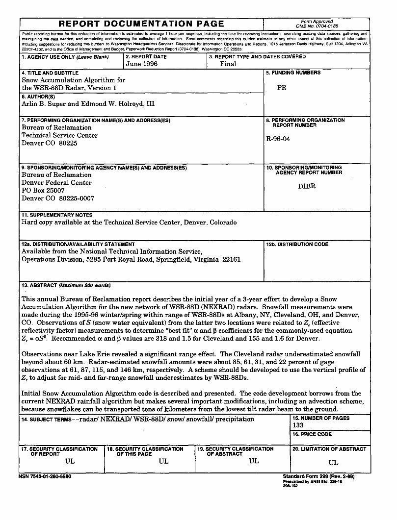
This annual Bureau of Reclamation report describes the initial year of a 3-year effort to develop a Snow Accumulation Algorithm for the new network of WSR-88D (NEXRAD) radars. Snowfall measurements were made during the 1995-96 winterlspring within range of WSR-88Ds a t Albany, NY, Cleveland, OH, and Denver, CO. Observations of S (snow water equivalent) from the latter two locations were related to 2, (effective reflectivity factor) measurements to determine "best fit" a and f! coefficients for the commonly-used equation 2, = dP. Recommended CY and f! values are 318 and 1.5 for Cleveland and 155 and 1.6 for Denver.

Observations near Lake Erie revealed a significant range effect. The Cleveland radar underestimated snowfall beyond about 60 km. Radar-estimated snowfall amounts were about 85,61,31, and 22 percent of gage observations a t 61,87,115, and 146 km, respectively. A scheme should be developed to use the vertical profile of 2, to adjust for mid- and far-range snowfall underestimates by WSR-88Ds.

Initial Snow Accumulation Algorithm code is described and presented. The code development borrows from the current NEXRAD rainfall algorithm but makes several important modifications, including an advection scheme, because snowflakes can be transported tens of kilometers from the lowest tilt radar beam to the ground. 14. SUBJECT TERMS- -radar/ NEXRADI WSR-88Dl snow/ snowfall1 precipitation 15. NUMBER OF PAGES 1 133

16. PRICE CODE

I I I

ISN 7540-01-280-5500 Standard Form 298 (Rev. 2-89) Pmsfbed by ANSI Std. 23918 296102

I

17. SECURITY CLASSIFICATION OF REPORT

18. SECURITY CLASSIFICATION 19. SECURIN CLASSIFICATION 20. LIMITATION OF ABSTRACT OF THIS PAGE OF ABSTRACT

SNOW ACCUMULATION ALGORITHM FOR THE WSR-88D RADAR,

VERSION 1

Arlin B. Super and Edmond W. Holtoyd, Ill

River Systems and Meteorology Group Water Resources Services

Technical Service Center Denver, Colorado

June 1996

UNITED STATES DEPARTMENT OF THE INTERIOR * BUREAU OF RECLAMATION

ACKNOWLEDGMENTS

It is no surprise that the efforts of many individuals were required in various aspects of special datacollection or analyses which culminated in this report. Jerry Klazura provided outstanding MOUmonitoring, often suggesting sources for technical information and assistance. Other NEXRADOperational Support Facility personnel who were helpful in particular aspects of the research includeJoe Chrisman, Tim O'Bannon, Bill Urell, and Colonels Tim Crum and Andy White.

Several National Weather Service personnel from the Albany, NY, Cleveland, OH, and Denver, CO,WFOs made special efforts on behalf of collecting quality observations. Notable among these are JohnQuinlan (Albany), Bob LaPlante and Frank Kieltyka (Cleveland), and David Imy and Mike Holzinger(Denver). The three WFO MIC's deserve special thanks for allowing their staffs to assist in the snowalgorithm efforts.

John Kobar and Neal Lott of the National Climatic Data Center promptly furnished the many LevelII data tapes that were requested for snow algorithm development.

The people who were interested enough in this project to collect special snowfall observations alldeserve acknowledgement. Those from the Albany area are too numerous to mention because about90 volunteer observers were involved, but their efforts are certainly appreciated. Cleveland areaobservers, all of whom did a first-rate job, are Mike Bezoski, Doug Brady, David Henderson, AnthonyMarshall, and Paul Mechling. The two Denver observers who deserve special mention for providinghigh quality hourly observations in addition to operating Belfort gages are Malcolm Bedell andRichard Kissinger. Steve Becker and Marc Jones provided quality gage measurements west of Denver.

Special appreciation is expressed to Dr. James Heimbach of the University of North Carolina atAsheville. Besides providing significant counsel and being the main source of rawinsonde datathroughout the field season, Dr. Heimbach found time in his busy schedule to program and rigorouslytest the optimization scheme used to determine radar equation coefficients, all without any monetarycompensation. His considerable and generous help is very much appreciated and will not be forgotten.

Dr. Paul Smith of the South Dakota School of Mines and Technology provided significant experttechnical advice to Reclamation scientists. Dr. Smith carefully read the first draft of this report andmade many helpful comments that improved it.

Jack McPartland of Reclamation was deeply involved in all aspects of site selection, gage calibrationand installation, and observer training. Curt Hartzell of Reclamation coordinated the collection ofdata needed for future storm partitioning. Ra Aman developed much of the programming for dealingwith Level II data on a Sun workstation. Besides writing several programs used in data handling,Anne Reynolds carefully reduced most of the numerous Belfort gage charts and then double-checkedthem all, an exceptionally tedious job requiring extraor4inary care and patience.

Special thanks are due Dave Matthews and Jim Pierce of Reclamation for providing additionalresources and a flexible environment for accomplishment of this work.

This work was primarily supported by the WSR-88D Operational Support Facility and the NextGeneration Weather Radar (NEXRAD) Program, with additional support by Reclamation's TechnicalService Center.

11

u.s. Department of the InteriorMission Statement

ABthe Nation's principal conservation agency, the Department of theInterior has responsibility for most of our nationally-owned publiclands and natural resources. This includes fostering sound use of ourland and water resources; protecting our fish, wildlife, and biologicaldiversity; preserving the environmental and cultural values of ournational parks and historical places; and providing for the enjoymentof life through outdoor recreation. The Department assesses ourenergy and mineral resources and works to ensure that theirdevelopment is in the best interests of all our people by encouragingstewardship and citizen participation in their care. The Departmentalso has a major responsibility for American Indian reservationcommunities and for people who live in island territories under U.S.administration.

The information contained in this report regarding commercialproducts or firms may not be used for advertising or promotionalpurposes and is not to be construed as an endorsement of anyproduct or firm by the Bureau of Reclamation.

iii

CONTENTS

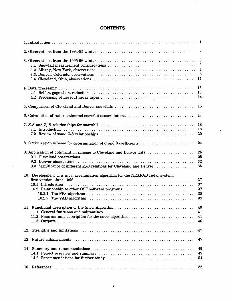
1. Introduction. . . . . . . . . . . . . . . . . . . . . . . . . . . . . . . . . . . . . . . . . . . . . . . . . . . . . . . . . . . . . .

2. Observations from the 1994-95 winter. . . . . . . . . . . . . . . . . . . . . . . . . . . . . . . . . . . . . . . . . .

3. Observations from the 1995-96 winter. . . . . . . . . . . . . . . . . . .. . . . . . . . . . . . . . . . . . . . . . . .3.1 Snowfall measurement considerations. . . . . . . . . . . . . . . . . . . . . . . . . . . . . . . . . . . . . .3.2. Albany, New York, observations. . . . . . . . . . . . . . . . . . . . . . . . . . . . . . . . . . . . . . . . . .3.3. Denver, Colorado, observations. . . . . . . . . . . . . . . . . . . . . . . . . . . . . . . . . . . . . . . . . . .3.4. Cleveland, Ohio, observations. . . . . . . . . . . . . . . . . . . . . . . . . . . . . . . . . . . . . . . . . . .

4. Data processing. . . . . . . . . . . . . . . . . . . . . . . . . . . . . . . . . . . . . . . . . . . . . . . . . . . . . . . . . .4.1 Belfort gage chart reduction. . . . . . . . . . . . . . . . . . . . . . . . . . . . . . . . . . . . . . . . . . . .4.2 Processing of Level II radar tapes. . . . . . . . . . . . . . . . . . . . . . . . . . . . . . . . . . . . . . . .

5. Comparison of Cleveland and Denver snowfalls. . . . . . . . . . . . . . . . . . . . . . . . . . . . . . . . . .

6. Calculation of radar-estimated snowfall accumulations. . . . . . . . . . . . . . . . . . . . . . . . . . . .

7. Z-S and Z.-S relationships for snowfall. . . . . . . . . . . . . . . . . . . . . . . . . . . . . . . . . . . . . . . .7.1 Introduction.. . . . . . . . . . . . . . . . . . . . . . . . . . . . . . . . . . . . . . . . . . . . . . . . . . . . . . .7.2 Review of some Z-S relationships. . . . . . . . . . . . . . . . . . . . . . . . . . . . . . . . . . . . . . . .

8. Optimization scheme for determination of a and ~coefficients. . . . . . . . . . . . . . . . . . . . . . .

9. Application of optimization scheme to Cleveland and Denver data. . . . . . . . . . . . . . . . . . . .9.1 Cleveland observations. . . . . . . . . . . . . . . . . . . . . . . . . . . . . . . . . . . . . . . . . . . . . . . .9.2 Denver observations. . . . . . . . . . . . . . . . . . . . . . . . . . . . . . . . . . . . . . . . . . . . . . . . . .9.3 Significance of different Z.-S relations for Cleveland and Denver. . . . . . . . . . . . . . . . .

10. Development of a snow accumulation algorithm for the NEXRAD radar system,first version: June 1996 . . . . . . . . . . . . . . . . . . . . . . . . . . . . . . . . . . . . . . . . . . . . . . . . . .. 3710.1 Introduction.. . .. . . . . . . . . . . . . . . . . . . . . . . . . . . . . . . . . . . . . . . . . . . . . . . . . .. 3710.2 Relationship to other OSF software programs. . . . . . . . . . . . . . . . . . . . . . . . .. . . .. 37

10.2.1 The PPS algorithm. . . . . . . . . . . . . . . . . . . . . . . . . . . . . . . . . . . . . . . . . . . . . . . 3810.2.2 The VAD algorithm. . . . . . . . . . . . . . . . . . . . . . . . . . . . . . . . . . . . . . . . . . . . .. 39

11. Functional description of the Snow Algorithm. . . . . . . . . . . . . . . . . . . . . . . . . . . . . . . . . .11.1 General functions and subroutines. . . . . . . . . . . . . . . . . . . . . . . . . . . . . . . . . . . . . .11.2 Program unit description for the snow algorithm. . . . . . . . . . . . . . . . . . . . . . . . . . . .11.3 Outputs '.' .

12. Strengths and limitations. . . . . . . . . . . . . . . . . . . . . . . . . . . . . . . . . . . . . . . . . . . . . . . . .

13. Future enhancements. . . . . . . . . . . . . . . . . . . . . . . . . . . . . . . . . . . . . . . . . . . . . . . . . . . .

14. Summary and recommendations. . . . . . . . . . . . . . . . . . . . . . . . . . . . . . . . . . . . . . . . . . . .14.1 Project overview and summary. . . . . . . . . . . . . . . . . . . . . . . . . . . . . . . . . . . . . . . . .14.2 Recommendations for further study. . . . . . . . . . . . . . . . . . . . . . . . . . . . . . . . . . . . . .

15. References............................................................

v

1

2

3346

11

131314

15

17

181820

24

25253235

40414146

47

47

494954

55

Appendix

Table

Figure

APPENDIXES

ABCDE

Optimization technique used to derive the Ze-S algorithm. . . . . . . . . . . . . . . . . . . . . .Algorithm documentation requirements. . . . . . . . . . . . . . . . . . . . . . . . . . . . . . . . . . . .Criteria for acceptance of deliverables ,.....Tasks of the MOD. . . . . . . . . . . . . . . . . . . . . . . . . . . . . . . . . . . . . . . . . . . . . . . . . . . .Production of the site-specific files used by the Snow Algorithm in theJune 1996version. . . . . . . . . . . . . . . . . . . . . . . . . . . . . ~ . . . . . . . . . . . . . . . . . . . . .. 79Program OCCTRIM . . . . . . . . . . . . . . . . . . . . . . . . . . . . . . . . . . . . . . . . . . . . . . . . . .. 85Program' HYSTRIMT . . . . . . . . . . . . . . . . . . . . . . . . . . . . . . . . . . . . . . . . . . . . . . . . .. 89Program POLAR230 , 99Program FLIPBYTE , 105Comparison between OSF and Reclamation routines. . . . . . . . . . . . . . . . . . . . . . . . .. 109Program RDNX.C , 115

57636973

FGHIJK

TABLES

12

Locations of two Belfort gage sites in the Albany area. . . . . . . . . . . . . . . . . . . . . . . . .. 5Summary of snow storm periods sampled by the volunteer network near Albany,New York, during the 1995-96 winter. . . . . . . . . . . . . . . . . . . . . . . . . . . . . . . . . . . . .. 6Locations of six snow observing sites in the Denver area. . . . . . . . . . . . . . . . . . . . . . .. 8Summary of significant snowstorm periods sampled by Belfort gages and snowboardsnear Denver, Colorado, during the 1995-96 winter. . . . . . . . . . . . . . . . . . . . . . . . . . .. 11Locations of five Belfort gage sites in the Cleveland area. . . . . . . . . . . . . . . . . . . . . .. 12Summary of significant snowfall periods sampled by Belfort gages east-northeastof Cleveland, Ohio, during the 1995-96 winter. . . . . . . . . . . . . . . . . . . . . . . . . . . . . .. 13Summary of snow water equivalents for 5 Cleveland gages for the first 2.monthsof the winter, and for 5 Denver gages for the first 3 months of the winter. . . . . . . . .. 16Summary of results of applying the optimization scheme to the five gages locatedeast-northeast ofCleveland. . . . . . . . . . . . . . . . . . . . . . . . . . . . . . . , . . . . . . . . . . .

" 26Summary of applying equation (8) to the data set from each Cleveland area gage. . . . . 27Summary of results of applying the optimization scheme to five gages inthe Denver area. . . . . . . . . . . . . . . . . . . . . . . . . . . . . . . . . . . . . . . . . . . . . . . . . . . . .. 32

34

56

7

8

910

FIGURES

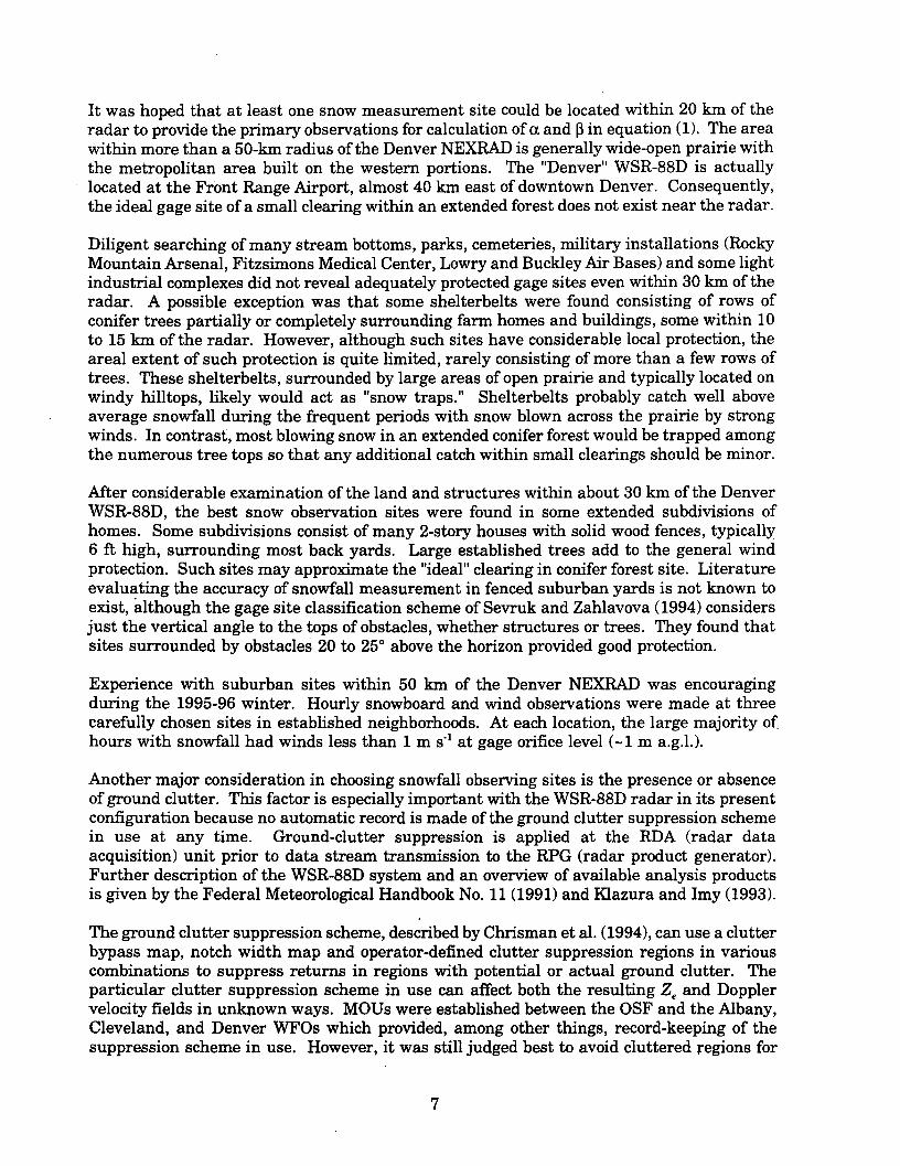
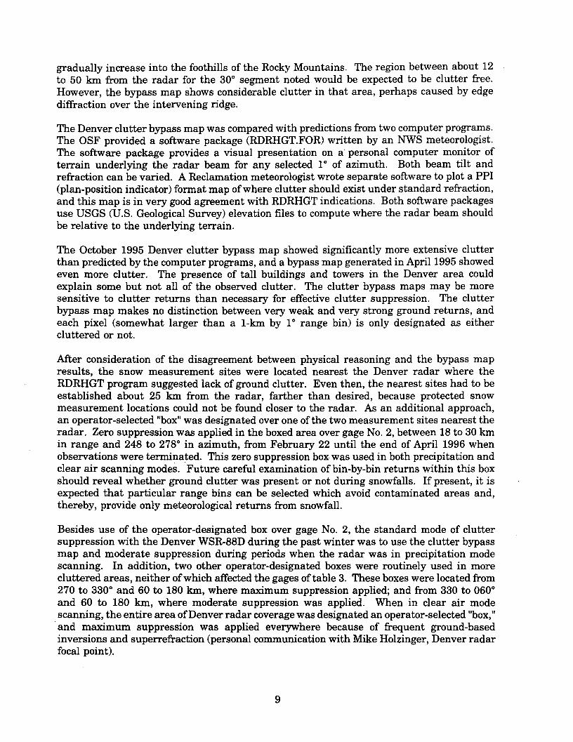
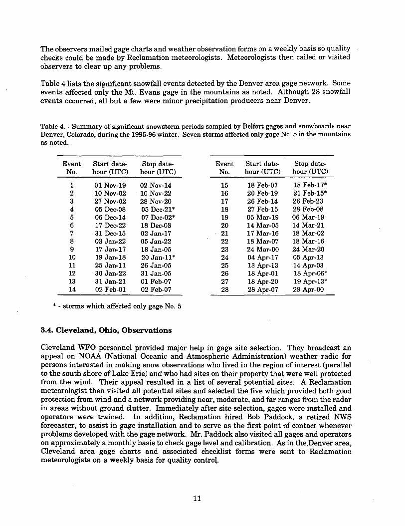
1 Plots of three different Ze-S relationships showing the effect of varying the13coefficient while the excoefficient remains constant. . . . . . . . . . . . . . . . , . . . . . . . . .Plots of three different Z.-S relationships showing the effect of varying theexcoefficient while the 13coefficient remains constant. . . . . . . . '. . . . . . . . . . . . . . . . . .Scatter plot of 143 pairs of hourly-observed snowfall for Cleveland gage No.1versus radar-estimated snowfall directly overhead using the relation Z. = 318 S1.5 . . . .Similar to figure 3 except for 235 pairs for Cleveland gage No.2. . . . . . . . . . . . . . . . .Similar to figure 3 except for 187 pairs for Cleveland gage No.3. . . . . . . . . . . . . . . . .Similar to figure 3 except for 202 pairs for Cleveland gage No.4. . . . . . . . . . . . . . . . .Similar to figure 3 except for 218 pairs for Cleveland gage No.5. . . . . . . . . . . . . . . . .Scatter plot of 196 pairs of hourly-observed snowfall for Denver gages No.1 to 3versus radar-estimated snowfall directly overhead using the relation Z. = 155 S1.6 . . . .Similar to figure 8 except the Cleveland Ze-S relationship of figure 3 isdeliberately misapplied to Denver gages No.1 to 3

""""""""""""'"Similar to figure 9 except that the Denver Z.-S relationship of figure 8 isdeliberately misapplied to Cleveland gages No.1 and 2 ,..... 36

222

223

45678

2528282929

349

3610

vi

1. Introduction

The OSF (Operational Support Facility) of the WSR-88D Radar Program released a requestfor proposals in the fall of 1994 seeking development of a snow accumulation algorithm forthe new national network of Doppler weather radars. Reclamation (Bureau of Reclamation)submitted a proposal in mid-October 1994, which was evaluated along with proposals fromother Federal and Federally-supported agencies. An MOV (memorandum of understanding)was signed the end of May 1995 among the NEXRAD (NEXt generation RADar) Program,the WSR-88D OSF, and Reclamation, which called for Reclamation to develop an algorithmover a 3-year period to estimate both S (snow water equivalent) and SD (snow depth) fromradar measurements. (Snow depth is sometimes called snow accumulation-in this report,snowfall accumulation refers to S accumulation for 1 hour or more.) This snow accumulation

.algorithm (hereafter Algorithm) is to be limited to dry snowfall. The complications of dealingwith mixed rain and snow and/or melting snow with associated "bright band" effects isbeyond the scope of the requested work and the resources available to accomplish it.

The original MOV was amended in August 1995 to include precipitation data collectionparallel to the south shore of Lake Erie east-northeast of the Cleveland, Ohio, WSR-88Dradar. Subsequent analysis of these snowfall and radar measurements was expected toevaluate the ability of the developing Algorithm to detect and quantify lake effect snowfalL

This report discusses progress during the first year of effort ending June 1, 1996. Threeletter-type quarterly reports have been submitted to the OSF which provide more detail aboutsome efforts.

This report is organized around the tasks to be performed by Reclamation scientists duringthe first year ending May 31, 1996, as spelled out in the MOV's SOW (statement of work).Briefly, the MOV tasks are:

1. Scrutinize existing precipitation gage observations of S from the 1994-95 winter withinreasonable range of WSR-88D systems with Level II data. Level II data, recorded on8-m~ tape, are the most basic data available to researchers (Crum et aI., 1993).

2. Obtain Level II data from selected WSR-88D systems and storm periods for the 1994-95winter that have corresponding gage data. Also obtain supporting software from the OSFfor manipulation of these data and hardware suitable for working with these data andsoftware. Progress under tasks No.1 and 2 is discussed in section 2 of this report.

3. Vse the data, software, and hardware of tasks No.1 and 2 above and write additionalsoftware as needed for development of a "simplified prototype" Algorithm for predictionof S from WSR-88D Level II data. The initial Algorithm will be based on comparisons ofradar measurements of equivalent (also called effective) reflectivity factor, Ze' with surfacegage measurements of S. The Algorithm will incorporate radar-estimated horizontal windspeed and direction for advection of falling snow particles to match surface observationsof S with radar bin observations of Ze. A large number of Ze-S pairs will be used tocalculate the empirically-determined coefficients, a. and ~, for the commonly-used power-law model:

Z = a.S~e. (1)

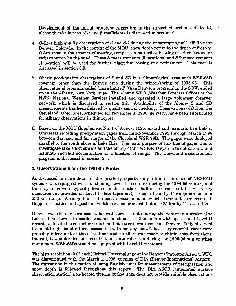
Development of the initial prototype Algorithm is the subject of sections 10 to 13,although calculations of a and ~ coefficients is discussed in section 9.

4. Collect high-quality observations of Sand SD during the winter/spring of 1995-96 nearDenver, Colorado. In the context of the MOU, snow depth refers to the depth of freshly-fallen snow in the absence of melting, compaction by surface heating or other factors, orredistribution by the wind. These S measurements (5 locations) and SD measurements(1 location) will be used for further Algorithm testing' and refinement. This task isdiscussed in section 3.3.

5. Obtain good-quality observations of Sand SD in a climatological area with WSR-88Dcoverage other than the Denver area during the winter/spring of 1995-96. Thisobservational program, called "more limited" (than Denver's program) in the SOW, endedup in the Albany, New York, area. The Albany WFO (Weather Forecast Office) of theNWS (National Weather Service) installed and operated a large volunteer observernetwork, which is discussed in section 3.2. Availability of the Albany Sand SDmeasurements has been delayed by quality control checking. Observations of S from theCleveland, Ohio, area, scheduled for November 1, 1996, delivery, have been substitutedfor Albany observations in this report.

6. Based on the MOU Supplement No.1 of August 1995, install and maintain five BelfortUniversal recording precipitation gages from mid-November 1995 through March 1996between the near and far ranges of the Cleveland WSR-88D. The gages were deployedparallel to the south shore of Lake Erie. The main purpose of this line of gages was toinvestigate lake effect storms and the ability of the WSR-88D system to detect snow andestimate snowfall accumulation as a function of range. The Cleveland measurementprogram is discussed in section 3.4.

2. Observations from the 1994.95 Winter

As discussed in more detail in the quarterly reports, only a limited number of NEXRADsystems was equipped with functioning Level II recorders during the 1994-95 winter, andthose systems were typically located in the southern half of the continental U.S. A keymeasurement provided on Level II data tapes is Ze for each l-km by 10 range bin out to a230-km range. A range bin is the basic spatial unit for which these data are recorded.Doppler velocities and spectrum width are also provided, but at O.25-km by 10 resolution.

Denver was the northernmost radar with Level II data during the winter in question (theBoise, Idaho, Level II recorder was not functional). Other radars with operational Level IIrecorders, located even farther south and at lower elevations than Denver, likely observedfrequent bright band returns associated with melting snowflakes. Dry snowfall cases wereprobably infrequent at those locations and no effort was made to obtain data from them.Instead, it was decided to concentrate on data collection during the 1995-96 winter whenmany more WSR-88Ds would be equipped with Level II recorders.

The high-resolution (O.OI-inch) Belfort Universal gage at the Denver (Stapleton Airport) WFOwas discontinued with the March 1, 1995, opening of DIA (Denver International Airport).The convention in this nation of using English units for measurement of precipitation andsnow depth is followed throughout this report. The DIA ASOS (automated surfaceobservation station) non-heated tipping bucket gage does not provide suitable observations

2

for Algorithm development. Reclamation scientists did acquire the existing Novemberthrough February Denver WFO hourly snowfall data, as well as daily snowfall amounts fromall cooperative observer gages within range of the Denver radar.

Besides the problem of sparsity of Denver data during the dry winter of 1994-95, it wasdiscovered that the standard mode of operation that winter was not to use the Clutter BypassMap. Rather, because of frequent ground-based inversions and superrefraction, maximumsuppression was routinely applied to the entire radar area of coverage. Communication withOSF specialists has revealed that suppression application might have commenced with radialwind speeds (i.e., toward or away from the radar) as great as 10 knots. Suppression isincreased as the radial wind speed decreases (Chrisman et aI., 1994). Radial winds less than10 knots are not uncommon over large portions of the lowest tilt radar beam (0.5° elevationangle) during many Denver-area winter storm periods. Consequently, meteorological returnswere likely often suppressed even in regions without ground clutter. With the uncertaintyof how much suppression was applied at a given place and time and the scarcity of surfacesnowfall observations it is difficult to see how much use can be made of 1994-95 winter datafrom Denver for establishing a Ze-S relationship. However, some attempts were made.

All hourly precipitation data from the Denver WFO were examined for the three snowstormsof the 1994-95 winter with associated Level II data. The only hourly values of record areTrace, 0.01, 0.02 and 0.06 (1 value only) inches, so the available range is very limited.Comparisons of these data with Ze values directly above the WFO gage revealed large scatter.The scatter was possibly caused in part by over-application of clutter suppression andpartially by the lack of range in the snowfall observations.

Twenty-four-hour precipitation totals from all area cooperative observer gages were alsoexamined and compared to Ze values directly overhead. This comparison resulted in evenlarger scatter than that observed with the Denver WFO hourly data. At that point, it wasdecided that resources would be better spent working with the upcoming 1995-96 winterobservations than dealing further with the limited and uncertain measurements from theprior winter.

3. Observations from the 1995.96 Winter

3.1 Snowfall Measurement Considerations

Accurate snowfall measurement is difficult because wind effects can cause significant tosevere gage undercatch as demonstrated by several authors over many decades. For example,Goodison (1978) reported that gage undercatch by an un shielded Belfort Universal gage canexceed 50 percent with wind speeds as low as 2.5 m s-l, and 75 percent with a 7-m S-l wind.Furthermore, Goodison showed that even a Belfort gage equipped with an Alter wind shieldcan exceed 50-percent undercatch with a 5 m S.l wind speed. Goodison and others haveshown that the degree of undercatch is even greater for some gage types, including theFisher-Porter, because of their shape.

Another problem is that many existing recording gages in the national network are of theFisher-Porter type with resolution of only 0.10-inch water equivalent. This resolution is anorder of magnitude less than the 0.01 inch (or less) provided by a Belfort gage. In mostregions of the U.S. which commonly experience snowfall, only a small fraction of all snowfallhours have a melted water equivalent of 0.10 inch or more. The infrequent occurrence of

3

higher rates is demonstrated for the Cleveland and Denver areas in section 5. Therefore,Fisher-Porter gages have little utility for relating radar observations to hourly snowfallobservations.

Even if snowboards are used to manually measure snowfall and are set flush with the snowor ground surface, windy sites can result in drifting of additional snow onto them or scouringof snow off of them. Windy sites must be avoided for quantitative snowfall measurements.

Because of the problems noted and others discussed by Groisman and Legates (1994), theexisting national precipitation gage network was determined at the onset to be inadequatefor the purposes ofthis study. Most climatological gages are read daily and, therefore, do nothave the needed time resolution. Many recording gages with hourly time resolution do nothave the desired mass resolution for snowfall (O.Ol-inch melted water equivalent or less).Tipping bucket gages usually can resolve 0.01 inch of water, but most are unheated so theycannot measure snowfall with any reasonable accuracy. And even where gages with adequatemass resolution exist, they tend to be located near WFOs, typically at wide-open, windyairports. The undercatch of such gages can be serious and unknown in magnitude. Snowfallmeasurements from such locations can add considerable variability to attempts to relatesnowfall accumulation to radar observations.

Small clearings in widespread conifer forest generally provide excellent snowfallmeasurement sites (e.g., Brown and Peck, 1962). Clearings in thick deciduous forest,especially if low brush is common, can also provide well-protected snowfall observing sites.Such forest clearings, together with gage wind shields, can almost eliminate gage undercatchcaused by airflow around the gage orifice. Gages installed and operated for this study wereplaced in forest clearings wherever possible. Of course, most of the U.S. does not havewidespread forest, and alternatives needed to be found for protecting gages from the wind inthe absence of forest. As will be discussed, different approaches to attempting to solve thesnowfall measurement problem were taken at each of at the three measurement areas(Albany, Cleveland, and Denver) during the 1995-96 winter.

It is desirable to locate snow observing sites intended for Ze-S comparisons as near the radaras practical. Such locations minimize the vertical distance between the radar beam and thesurface, which reduces uncertainties caused by wind advection of snow particles. In addition,the volume sampled by the radar increases with range as the beam broadens in width andheight. So the representativeness of a surface point observation for the overlying range binor bins becomes increasingly uncertain at more distant ranges. However, as a practicalmatter, these factors must be weighed against usually greater ground clutter contaminationnear the radar and whether suitable surface observing sites exist near the radar. Thetradeoffs involved in selecting a snow observing site near a radar are perhaps best illustratedin the discussion of site selection in the Denver area in section 3.3.

3.2. Albany, New York, Observations

Unlike the other two sites, Reclamation had a limited role in data collection within range ofthe Albany, New York, WSR-88D. Reclamation supplied one Belfort gage with an Alter windshield. John Quinlan, a forecaster at the Albany WFO, supplied another Belfort gage, andReclamation provided an Alter shield for that gage as well. These two gages, noted in table1, were installed by Albany WFO personnel. Reclamation also supported computer data entryof volunteer observations by university students.

4

Distance! Azim uthGage Location Latitude Longitude m.s.!. Elevation from Radar(Operator) (°_') (°_') (m) (kmr)*

Round Lake 42-55.430 73-47.152 59 44/31 °(J. Quinlan)East Durham(F. Stark) 42-20.095 74-03.038 136 28/178°

Table 1. - Locations of two Belfort gage sites in the Albany area.

* All azimuths are given in degrees (°) true in this report.

A large volunteer network was established around Albany largely through the efforts of JohnQuinlan. After advertising for volunteers, Mr. Quinlan met with potential snowfall observersto explain the project during a series of meetings around the area of radar coverage. Mr.Quinlan visited those persons with both the interest and a suitable location and gave theminstructions and the equipment necessary to make hourly observations of both Sand SD.Mr. Quinlan also took GPS (global positioning system) readings at each location to documentlatitude and longitude. About 90 volunteers were trained and equipped with appropriateforms for logging data, snowboards (1 by 1 ft), rulers graduated to the nearest 0.1 inch, andClear Vu Model 1100 rain gages. The latter were not used as gages, but the 4-inch-diameterouter shells with sharp tapered edges were used to core snow on boards after the SDmeasurement was made at the end of each hour. The cored sample was then melted indoorsand the measurement of S was made in the usual manner by pouring the melted water intothe 1-I/4-inch-diameter inner tube, which is graduated every 0.01 inch. Snowboardobservations are generally more accurate than gage observations unless gages are wellprotected from the wind.

Efforts were made to locate Albany network snowboards in reasonably protected locations,but local wind measurements were only made at sites with pre-existing anemometers. Somedrifting and scouring of snow from individual boards may have occurred during windier stormperiods and network observers in most instances noted this occurrence on the observationform or stopped taking observations at that time. The use of a large number of samplingpoints should partially compensate for wind-caused errors in the hourly snowboardmeasurements of Sand SD.

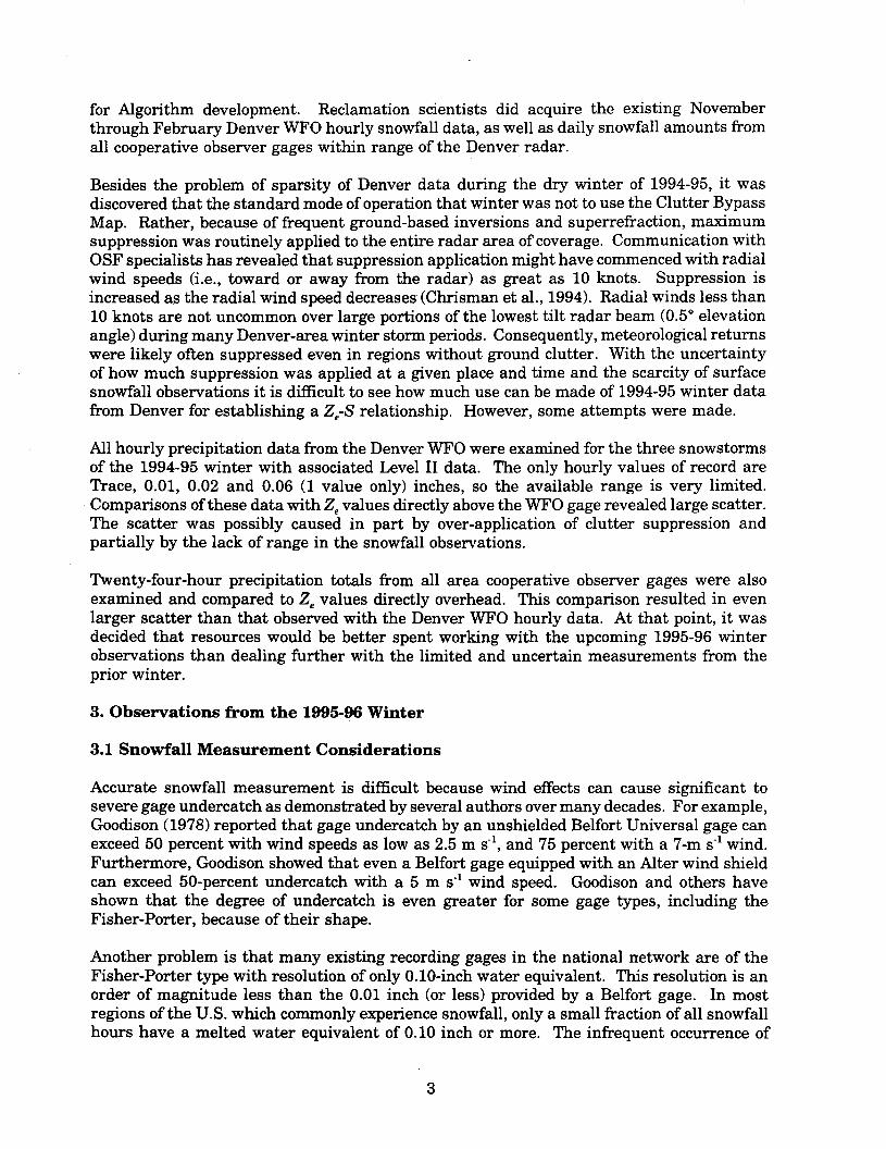
The Albany network was partially or fully activated by phone calls from the WFO on 13occasions from December 1,1995, through mid-April 1996 as noted in table 2 supplied by Mr.Quinlan. The start and stop times in table 2 include a couple of hours before and after actualsnowfall as each storm approached and left the Albany area. Partial or full networkactivation depended upon whether the Albany WFO forecasters expected only a portion or allofthe WSR-88D's area or coverage to be affected by an approaching storm. The network wasactivated only when forecasters expected dry snowfall without bright band effects.

5

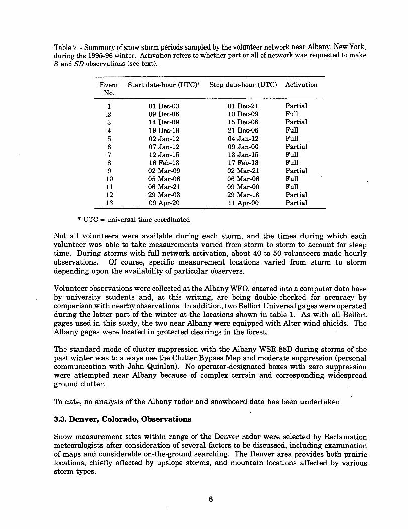
Table 2. -Summary of snow storm periods sampled by the volunteer network near Albany, New York,during the 1995-96 winter. Activation refers to whether part or all of network was requested to makeS and SD observations (see text).

EventNo.

Start date-hour (UTC)* Stop date-hour (UTC) Activation

1.2345678910111213

01 Dec-03

09 Dec-0614 Dec-0919 Dec-1802 Jan-1207 Jan-1212 Jan-1516 Feb-1302 Mar-0905 Mar-0606 Mar-2129 Mar-0309 Apr-20

01 Dec-21'10 Dec-0915 Dec-0621 Dec-0604 Jan-1209 Jan-OO13 Jan-1517 Feb-1302 Mar-2106 Mar-0609 Mar-OO29 Mar-1811 Apr-OO

PartialFullPartialFullFullPartialFullFullPartialFullFullPartialPartial

* UTC = universal time coordinated

Not all volunteers were available during each storm, and the times during which eachvolunteer was able to take measurements varied from storm to storm to account for sleeptime. During storms with full network activation, about 40 to 50 volunteers made hourlyobservations. Of course, specific measurement locations varied from storm to stormdepending upon the availability of particular observers.

Volunteer observations were collected at the Albany WFO, entered into a computer data baseby university students and, at this writing, are being double-checked for accuracy bycomparison with nearby observations. In addition, two Belfort Universal gages were operatedduring the latter part of the winter at the locations shown in table 1. As with all Belfortgages used in this study, the two near Albany were equipped with Alter wind shields. TheAlbany gages were located in protected clearings in the forest. .

The standard mode of clutter suppression with the Albany WSR-88D during storms of thepast winter was to always use the Clutter Bypass Map and moderate suppression (personalcommunication with John Quinlan). No operator-designated boxes with zero suppressionwere attempted near Albany because of complex terrain and corresponding widespreadground clutter.

To date, no analysis of the Albany radar and snowboard data has been undertaken.

3.3. Denver, Colorado, Observations

Snow measurement sites within range of the Denver radar were selected by Reclamationmeteorologists after consideration of several factors to be discussed, including examinationof maps and considerable on-the-ground searching. The Denver area provides both prairielocations, chiefly affected by upslope storms, and mountain locations affected by variousstorm types.

6

It was hoped that at least one snow measurement site could be located within 20 kIn of theradar to provide the primary observations for calculation of a and ~in equation (1). The areawithin more than a 50-kIn radius of the Denver NEXRAD is generally wide-open prairie withthe metropolitan area built on the western portions. The "Denver" WSR-88D is actuallylocated at the Front Range Airport, almost 40 kIn east of downtown Denver. Consequently,the ideal gage site of a small clearing within an extended forest does not exist near the radar.

Diligent searching of many stream bottoms, parks, cemeteries, military installations (RockyMountain Arsenal, Fitzsimons Medical Center, Lowry and Buckley Air Bases) and some lightindustrial complexes did not reveal adequately protected gage sites even within 30 kIn of theradar. A possible exception was that some shelterbelts were found consisting of rows ofconifer trees partially or completely surrounding farm homes and buildings, some within 10to 15 kIn of the radar. However, although such sites have considerable local protection, theareal extent of such protection is quite limited, rarely consisting of more than a few rows oftrees. These shelterbelts, surrounded by large areas of open prairie and typically located onwindy hilltops, likely would act as "snow traps." Shelterbelts probably catch well aboveaverage snowfall during the frequent periods with snow blown across the prairie by strongwinds. In contrast, most blowing snow in an extended conifer forest would be trapped amongthe numerous tree tops so that any additional catch within small clearings should be minor.

Mter considerable examination of the land and structures within about 30 kIn of the DenverWSR-88D, the best snow observation sites were found in some extended subdivisions ofhomes. Some subdivisions consist of many 2-story houses with solid wood fences, typically6 ft high, surrounding most back yards. Large established trees add to the general windprotection. Such sites may approximate the "ideal" clearing in conifer forest site. Literatureevaluating the accuracy of snowfall measurement in fenced suburban yards is not known toexist, although the gage site classification scheme of Sevruk and Zahlavova (1994) considersjust the vertical angle to the tops of obstacles, whether structures or trees. They found thatsites surrounded by obstacles 20 to 25° above the horizon provided good protection.

Experience with suburban sites within 50 kIn of the Denver NEXRAD was encouragingduring the 1995-96 winter. Hourly snowboard and wind observations were made at threecarefully chosen sites in established neighborhoods. At each location, the large majority of.hours with snowfall had winds less than 1 m S.l at gage orifice level (-1 m a.g.l.).

Another major consideration in choosing snowfall observing sites is the presence or absenceof ground clutter. This factor is especially important with the WSR-88D radar in its presentconfiguration because no automatic record is made of the ground clutter suppression schemein use at any time. Ground-clutter suppression is applied at the RDA (radar dataacquisition) unit prior to data stream transmission to the RPG (radar product generator).Further description of the WSR-88D system and an overview of available analysis productsis given by the Federal Meteorological Handbook No. 11 (1991) and Klazura and Imy (1993).

The ground clutter suppression scheme, described by Chrisman et al. (1994), can use a clutterbypass map, notch width map and operator-defined clutter suppression regions in variouscombinations to suppress returns in regions with potential or actual ground clutter. Theparticular clutter suppression scheme in use can affect both the resulting Ze and Dopplervelocity fields in unknown ways. MOUs were established between the OSF and the Albany,Cleveland, and Denver WFOs which provided, among other things, record-keeping of thesuppression scheme in use. However, it was still judged best to avoid cluttered regions for

7

m.s.I. Distance/AzimuthGage Location Gage Latitude Longitude Elevation from Radar(Operator) No. (°.') (°.') (m) (kml°)*

SE Aurora 1 39-38.217 104-46.206 1758 25/229(M. Bedell)NE Aurora 2 39-45.609 104-49.322 1631 24/263(R. Kissinger)Lakewood 3 39.41.272 105-06.282 1703 49/257(A. Super)Pine Valley 4 39-24.400 105-20.843 2100 81/239(S. Becker)Mt. Evans 5 39-39.316 105-35.642 3265 91/261(M. Jones)Black Forest 6 39.01.720 105-40.908 2295 85/188(J. Bishop) (no data until late January)

gage locations so the Zevalues over the gages were both uncluttered and uncontaminated byclutter suppression. One deliberate exception (Mt. Evans in table 3) provided data withwhich to evaluate the WSR-BBDs ability to detect snowfall over rugged mountains.

Table 3. - Locations of six snow observing sites in the Denver area. The three sites located nearestthe radar had both Belfort gages and hourly snowboard readings. Latitudes and longitudes weremeasured by GPS, and elevations were estimated from a USGS (U.S. Geological Survey) data base orlarge-scale maps.

Clutter bypass maps were obtained from the three radars in question and plotted on1:500,000 scale topographic maps of each area. A clutter bypass map shows where groundclutter was detected by the radar during the particular few hours of special observation. Themap is attempted to be made under well-mixed atmospheric conditions with no precipitationpresent. The bypass map is expected to approximate the clutter pattern during standardrefraction. Actually, two maps are generated, one for the two lowest antenna tilts (0.5 and1.5°) and the other for all higher scan angles. All future references will be to the former mapbecause Ze values from only the lower tilt were used in. the analysis to be discussed.

Unfortunately, clutter bypass maps are not generated to the same 1° by l-km resolution as. Ze data but are generated on a coarser 256-radial by 360° pixel grid. In addition to the

problem of the mismatch in Ze and clutter bypass map coordinates, the bypass map tends to"smear" potentially cluttered regions. Much clutter is "point-target" echo (Paul Smith',.personal communication), which is probably over-emphasized by the bypass map pixel scale.

The Denver bypass map, generated in October 1995 and used throughout the 1995-96 winter,showed few continuous uncluttered areas within 30 km of the radar. The uncluttered areaswere located to the east and southeast where prairie exists with almost no tree cover orhousing developments to provide protection for snow measurements.

The extent of bypass map clutter at moderate ranges west of the Denver radar was surprisingbecause a minor ridge about 12 km distant for azimuths between about 250 and 2BO° (allazimuths are given in degrees [°] true in this report) reaches the bottom of the 0.5° tilt beam(the beam is 0.95° wide). This ridge would be expected to absorb any sidelobe energy underthe lowest elevation angle beams for which the lower clutter map is generated. Elevationsdecrease beyond the near ridge until about the 40-km range (South Platte River) and then

B

gradually increase into the foothills of the Rocky Mountains. The region between about 12to 50 km from the radar for the 300 segment noted would be expected to be clutter free.However, the bypass map shows considerable clutter in that area, perhaps caused by edgediffraction over the intervening ridge.

The Denver clutter bypass map was compared with predictions from two computer programs.The OSF provided a software package (RDRHGT.FOR) written by an NWS meteorologist.The software package provides a visual presentation on a' personal computer monitor ofterrain underlying the radar beam for any selected r of azimuth. Both beam tilt andrefraction can be varied. A Reclamation meteorologist wrote separate software to plot a PPI(plan-position indicator) format map of where clutter should exist under standard refraction,and this map is in very good agreement with RDRHGT indications. Both software packagesuse USGS (U.S. Geological Survey) elevation files to compute where the radar beam shouldbe relative to the underlying terrain.

The October 1995 Denver clutter bypass map showed significantly more extensive clutterthan predicted by the computer programs, and a bypass map generated in April 1995 showedeven more clutter. The presence of tall buildings and towers in the Denver area couldexplain some but not all of the observed clutter. The clutter bypass maps may be moresensitive to clutter returns than necessary for effective clutter suppression. The clutterbypass map makes no distinction between very weak and very strong ground returns, andeach pixel (somewhat larger than a l-km by 10 range bin) is only designated as eithercluttered or not.

Mter consideration of the disagreement between physical reasoning and the bypass mapresults, the snow measurement sites were located nearest the Denver radar where theRDRHGT program suggested lack of ground clutter. Even then, the nearest sites had to beestablished about 25 km from the radar, farther than desired, because protected snowmeasurement locations could not be found closer to the radar. As an additional approach,an operator-selected "box" was designated over one of the two measurement sites nearest theradar. Zero suppression was applied in the boxed area over gage No.2, between 18 to 30 kmin range and 248 to 2780 in azimuth, from February 22 until the end of April 1996 whenobservations were terminated. This zero suppression box was used in both precipitation andclear air scanning modes. Future careful examination of bin-by-bin returns within this boxshould reveal whether ground clutter was present or not during snowfalls. If present, it isexpected that particular range bins can be selected which avoid contaminated areas and,thereby, provide only meteorological returns from snowfall.

Besides use of the operator-designated box over gage No.2, the standard mode of cluttersuppression with the Denver WSR-88D during the past winter was to use the clutter bypassmap and moderate suppression during periods when the radar was in precipitation modescanning. In addition, two other operator-designated boxes were routinely used in morecluttered areas, neither of which affected the gages oftable 3. These boxes were located from270 to 3300 and 60 to 180 km, where maximum suppression applied; and from 330 to 0600and 60 to 180 km, where moderate suppression was applied. When in clear air modescanning, the entire area of Denver radar coverage was designated an operator-selected "box,"

.and maximum suppression was applied everywhere because of frequent ground-basedinversions and superrefraction (personal communication with Mike Holzinger, Denver radarfocal point).

9

Besides the two measurement sites at about 25 kIn from the radar, four other sites werechosen at greater distances as shown in table 3. As with the two nearest sites, the observinglocation at the 49-km range was located in an established neighborhood with solid fencedbackyards in a region that should not have had ground clutter. In addition to operation ofthe shielded Belfort gages at these three sites, hourly manual measurements were made ofSand SD on 1- by I-ft snowboards laid on the ground or snow cover near the gages. Thesame Clear Vu Model 1100 gages used in Albany were used to core snow on the boards afterfour depth measurements were made and averaged. Manual measurements were usuallymade from early morning until normal bedtime whenever snow was falling. Comparisons ofall hourly snowboard and gage observations from gages No.1 through 3 indicated that the3 operators were conscientious. Resulting correlation coefficients between S pairs exceeded0.96 for each data set.

.

Denver WFO personnel made special hourly observations of Sand SD whenever snowfalloccurred during the 1995-96 winter/spring. These measurements and the snowboardobservations from the 3 gage sites nearest the Denver WSR-88D have yet to be analyzed.

Three additional sites were chosen for operation of Belfort gages but not hourly snowboardobservations. However, snowboards were sampled in the same manner just discussed eachmorning after snowfall had occurred. This procedure provided comparisons with gagemeasurements and identified days with snowfall. The same practice was used at the fiveCleveland gages to be discussed.

All Belfort gages used in this study had accurate clocks that rotated once per 24 h, whichmeant the pen trace overwrote the same horizontal line until precipitation occurred. Theneed to identify days with precipitation is obvious. This identification was not difficultbecause gage operators filled out a worksheet each morning after snow or rain, noting currentweather conditions including wind speed at gage orifice level. A small Taylor wind speedmeter with a minimum indication of 2 mi h-1was used to measure wind speed.

Little data resulted from the Black Forest gage listed in table 3 until after late January 1996because of difficulties finding a reliable operator. The data quality from the other five gagesin the Denver area was generally very good. The three most distant gages were located inwell-protected clearings in conifer forest. The two gages well west of the radar were locatedin a large mountain valley, protected from ground clutter by upwind terrain, and in amountainous area where the lowest tilt beam intersects the terrain. The latter site, at 3265m altitude, was located at the Mt. Evans Research Station climatological station.Measurements from this location will be examined to determine if any useful snowfall.accumulation estimates can be made by radar in a very cluttered region. The 1.50 tilt beammay be usable for this purpose, but this estimate has yet to be attempted.

Five gage sites were operational by November 1, 1995. The sixth gage was also establishedby then, but reliable observations were not obtained until after late January when a new.operator was trained. Gages (all with Alter-type wind screens) were installed and calibrated,and antifreeze and other supplies were located at each site. Each observer received trainingconcerning gage servicing. The two observers nearest the radar received additional trainingin making hourly measurements of snow depth and in observing sizes and types ofthe largersnowflakes that provide almost all of the meteorological radar returns during snowfall. Thethird site with special hourly observations (Lakewood) was maintained by a Reclamationmeteorologist. A snow particle identification guide was prepared for use by hourly observers.

10

Event Start date- Stop date- Event Start date- Stop date-No. hour (UTC) hour (UTC) No. hour (UTC) hour (UTC)

1 01 Nov-19 02 Nov-14 15 18 Feb-07 18 Feb-17*2 10 Nov-02 10 Nov-22 16 20 Feb-19 21 Feb-15*3 27 Nov-02 28 Nov-20 17 26 Feb-14 26 Feb-234 05 Dec-08 05 Dec-21 * 18 27 Feb-15 28 Feb-085 06 Dec-14 07 Dec-02* 19 05 Mar-19 06 Mar-196 17 Dec-22 18 Dec-08 20 14 Mar-05 14 Mar-217 31 Dec-15 02 Jan-17 21 17 Mar-16 18 Mar-028 03 Jan-22 05 Jan-22 22 18 Mar-07 18 Mar-169 17 Jan-17 18 Jan-05 23 24 Mar-OO 24 Mar-20

10 19 Jan-18 20 Jan-11* 24 04 Apr-17 05 Apr-1311 25 Jan-11 26 Jan-05 25 13 Apr-13 14 Apr-0312 30 Jan-22 31 Jan-05 26 18 Apr-Ol 18 Apr-06*13 31 Jan-21 01 Feb-07 27 18 Apr-20 19 Apr-13*14 02 Feb-Ol 02 Feb-07 28 28 Apr-07 29 Apr-OO

* - storms which affeCted only gage No.5

3.4. Cleveland, Ohio, Observations

The observers mailed gage charts and weather observation forms on a weekly basis so qualitychecks could be made by Reclamation meteorologists. Meteorologists then called or visitedobservers to clear up any problems.

Table 4 lists the significant snowfall events detected by the Denver area gage network. Someevents affected only the Mt. Evans gage in the mountains as noted. Although 28 snowfallevents occurred, all but a few were minor precipitation producers near Denver.

Table 4. - Summary of significant snowstorm periods sampled by Belfort gages and snowboards nearDenver, Colorado, during the 1995-96 winter. Seven storms affected only gage No.5 in the mountainsas noted.

Cleveland WFO personnel provided major help in gage site selection. They broadcast anappeal on NOAA (National Oceanic and Atmospheric Administration) weather radio forpersons interested in making snow observations who lived in the region of interest (parallelto the south shore of Lake Erie) and who had sites on their property that were well protectedfrom the wind. Their appeal resulted in a list of several potential sites. A Reclamationmeteorologist then visited all potential sites and selected the five which provided both goodprotection from wind and a network providing near, moderate, and far ranges from the radarin areas without ground clutter. Immediately after site selection, gages were installed andoperators were trained. In addition, Reclamation hired Bob Paddock, a retired NWSforecaster, to assist in gage installation and to serve as the first point of contact wheneverproblems developed with the gage network. Mr. Paddock also visited all gages and operatorson approximately a monthly basis to check gage level and calibration. As in the.Denver area,Cleveland area gage charts and associated checklist forms were sent to Reclamationmeteorologists on a weekly basis for quality control.

11

m.s.!. Distance/AzimuthGage Location Gage Latitude Longitude Elevation from Radar(Operator) No. (°.') (°.') (m) (kmJ°)*

Highland Hts 1 41-33.126 81-28.348 292 36/64(A. Marshall)Chardon 2 41-36.712 81-10.382 359 61/69(D. Brady)Geneva 3 41-46.552 80-56.317 247 87/62(M. Bezoski)Pierpont 4 41-44.330 80-32.780 317 115/71(P. Mechling)Cranesville 5 41-55.299 80-14.301 373 146/67(D. Henderson)

The Cleveland approach worked very well. Selecting gage operators who showed definiteinterest in the project by responding to the NOAA weather radio appeal and hiring a part-time local meteorologist to oversee the project resulted in a high quality data set. Fewproblems were encountered with the Cleveland area gage network. The enthusiasm anddedication of all five gage operatprs and Mr. Paddock were remarkable.

Table 5 lists the five Belfort gage locations and gage operators. As with Albany and Denversites, latitudes and longitudes were determined by GPS, and altitudes were extracted froma terrain data base or large-scale maps.

Table 5. . Locations of five Belfort gage sites in the Cleveland area. Gages No.1 to 4 were located inOhio, and gage No.5 was located in northwestern Pennsylvania.

All five Cleveland area gages were brought to operational status during the first week ofNovember, well ahead of the mid-November schedule called for under this task. Snowstormsbegan affecting the gage network after the first three gages were installed. Because of recordsnowfalls in the area, many storm periods were observed by the gage network and by radar.Most were lake effect storms, but some general synoptic storms were also observed.

A listing of all storms that produced more than minor snowfall in the Belfort gage line isgiven in table 6. This table was prepared from a larger list supplied by Bob LaPlante andFrank Kieltyka of the Cleveland WFO which includes all snowfall events, some very minoralong the gage line. Messrs. LaPlante and Kieltyka classified each storm into one of threecategories: Major LES (lake effect storms), defined by production of at least 6 inches ofsnowfall in no more than 12 hours at 2 or more sites in a county; major synoptic storms; andother less prominent events which were not classified (mixture of minor lake effect stormsand "other"). The latter are called "Minor Events" in table 6, although some producedsignificant snow at one or more gages.

The standard method of clutter suppression with the Cleveland WSR-88D during the pastwinter was to use the clutter bypass map and moderate suppression except from November1 through December 4, 1995, when high suppression is believed to have been applied. Inaddition, an operator-designated box was established over the gage nearest the radar from.29 to 43 km and 53 to 75° azimuth. Zero suppression was applied within the box fromDecember 4, 1995, until the end of the field season (personal communication with BobLaPlante, Cleveland Science Operations Officer).

12

Table 6. - Summary of significant snowfall periods sampled by Belfort gages east-northeast ofCleveland, Ohio, during the 1995-96 winter.

Event Start date Stop date Storm Event Start date Stop date StormNo. -hour (UTC) -hour (UTC) Type No. -hour (UTC) -hour (UTC) Type

1 04 Nov-OO 05 Nov-05 Major LES 13 12 Jan-OO 13 Jan-04 Minor Event2 08 Nov-08 09 Nov-19 Major LES 14 24 Jan-12 25 Jan-05 Minor Event3 15 Nov-12 16 Nov-18 Major LES 15 30 Jan-12 31 Jan-06 Minor Event4 17 Nov-05 17 Nov-23 Minor Event 16 11 Feb-12 12 Feb-12 Minor Event5 21 Nov-11 22 Nov-16 Major LES 17 14 Feb-OO 15 Feb-07 Minor Event6 09 Dec-OO 12 Dec-17 Major LES 18 17 Feb-12 18 Feb-08 Minor Event7 19 Dec-06 20 Dec-04 Major Synoptic 19 28 Feb-18 01 Feb-OO Major LES8 20 Dec-lO 21 Dec-20 Major LES 20 02 Mar-12 03 Mar-04 Minor Event9 22 Dec-12 24 Dec-20 Minor Event 21 03 Mar-04 04 Mar-05 Major LES10 25 Dec-17 26 Dec-13 Major LES 22 08 Mar-23 09 Mar-12 Major LES11 02 Jan-14 04 Jan-OO Major Synoptic 23 01 Apr-OO 02 Apr-03 Minor Event12 09 Jan-21 10 Jan-14 Major LES

4. Data Processing

4.1 Belfort Gage Chart Reduction

Considerable care has been given to the time-consuming task of reducing Belfort gage charts.Clock accuracy was generally within 5 minutes per week or less, and charts were changedat least weekly. Start and stop times were carefully noted, and an additional mid-week timecheck was made as a minimum. Clocks which did not maintain an accuracy of 5 minutes perweek were adjusted (spring-wound clocks) or replaced (quartz-crystal electric clocks).

Charts were carefully read with at least 4-power magnification and good lighting to thenearest 0.005 inch at hourly intervals. The resolution claimed for the Belfort gage is 0.01inch, but pen trace movements of 0.005-inch magnitude are readily apparent with carefulexamination.

The "raw" chart reading was penciled in by each hour's line on the chart. Later, a secondcheck was made of each reading to detect any errors. After computer processing, hourlysnowfall accumulations were compared among neighboring gages and any obvious outlierswere checked yet again on the charts. Moreover, all high snowfall accumulations were givenan additional special check because they are uncommon but important in calculation of theoptimum Ze-S relationship.

Special attention was paid to chart readings near the daily time of chart overlap (0700-0800)because the extra thickness of the overlapping paper causes the pen to rise then fall over afew-hour period. The Belfort Charts No. 5-4047-B have a triple paper thickness whennormally installed (two end flaps with one folded over), but one flap was cut off to minimizethe vertical pen motion. Even then, readings near the overlap can be misleading if onesimply uses the chart readings; that is, the pen trace relative to the horizontal lines that areinked at 0.05-inch intervals on the charts. A better approach, which was used, is to comparethe differences in chart readings near the overlap with days having no precipitation. Because7 rotations (traces) were obtained on most charts, non-precipitation periods were almost

. always available to compare against. Changes in the differences hour by hour provided thebest estimate of snowfall accumulation near times of chart overlap. The raw chart readingwas used at other times. These raw readings were entered into a computer file and aprogram was written to calculate hourly differences. Because charts were operated in local

13

time to avoid confusing the operators, the program also listed both local and UTC (universaltime coordinated) date and hours because radar data are recorded in UTC time.

Some data losses occasionally occurred, usually because of clock stoppages or gagemalfunctions. The only major data loss was the previously discussed Black Forest gage southof Denver. Overall, the gage record is considered to be of very good quality, both because ofcareful locating of gages so they were protected from the wind and because of considerablecare taken to calibrate and maintain the gages and in chart reduction.

4.2 Processing of Level II Radar Tapes

Copies of original Level II 8-mm Exabyte tapes from the Albany, Cleveland, and Denverradars have been, or will be, obtained from the NCDC (National Climatic Data Center) inAsheville, North Carolina, for all periods with significant snowfalls. Tape processing wasdone with a Sun Spare 20 workstation under the Solaris 2.4 operating system. The first stepwas to use a routine that extracted each file's start and stop times and size and then closedthe file. The resulting file directory from this initial processing provides the means todetermine exactly which files are needed from each tape to match snowstorm periods in laterprocessing.

File number 1 on Level II tapes contains header information and numbers 2 to 401 are datafiles unless recording is interrupted before the last file, 401, is written. One volume scan isusually equivalent to one file although occasionally two volume scans are erroneously writtento a single file. Software has not yet been developed to extract the second file in such cases.Occasionally, a short file is written which may contain little but header information andperhaps part of a volume scan. All files less than 4 minutes in duration were ignored in laterprocessmg.

File size indicates scan strategy. For example, a typical precipitation mode volume scan (seeFederal Meteorological Handbook No. 11,1991) during snowfall requires about 5.75 minutesand produces a 9.8-megabyte file. Clear air volume scans take almost 10 minutes andproduce somewhat smaller files.

The second step in processing is to open only the desired files on each tape and save thefraction of the total information needed for comparison with snow observations. The Zevalues, recorded to the nearest 0.5 dBZ, where dBZ = 10 LogZe, were extracted for two arraysof range bins over each snow measurement site from the lowest (0.5°) beam. One array wascentered directly over the site (so-called "vertical" array) as though snow fell verticallywithout advection. The other array was advected by the wind (so-called "upwind" array) inan attempt to make a more realistic match between gage position and the region of the 0.5°radar beam from which the snow actually fell.

For each type of array and each snow measurement site, dBZ values were extracted oversemi-equal areas. Each array consisted of a "box" exactly 3 km in range (depth) by at least3 km in azimuth (width). A minimum of 3° of azimuth was always used so the azimuthalwidth was greater than 3 km at ranges exceeding 60 km where 1° equals 1 km in width (e.g.,three 1° radials result in a 6-km width at a 120-km range). The smallest array was,therefore, 3 x 3 = 9 range bins. For ranges nearer to the radar than about 50 kIn, additionalradials were added to the array to maintain an approximate 3-km width. Radials were addedin steps of two to keep an odd number (5, 7, 9, . . .) of degrees azimuth by a 3-kIn range in

14

the array. Because the recorded radial azimuth values vary from scan to scan, the exactazimuthal position of the array over a gage also varied slightly. In contrast, range wasalways fixed with the center of each range bin exactly at 0.5, 1.5, 2.5, . . . km from the radar.In any event, all vertical arrays were chosen so that the gage was always positioned directlybelow the center range bin of the array.

For the purpose of extracting upwind arrays, VAD (vertical azimuth display) winds werecalculated at 1000-ft intervals for each volume scan (file) as discussed in section 10.2. Thisprocess simulates the standard WSR-88D VAD product, which portrays winds in 1000-ftintervals. The wind information was used to advect the falling particles. Snowflake fallspeed observations are not made with the WSR-88Ds. Although the Doppler shift could beused to estimate particle fall speeds, a different scan strategy would be required, including.an almost vertical antenna tilt. In the absence of fall speed measurements, the largersnowflakes, which produce almost all the returned signal (Ze)' were assumed to fall at exactly1.0 m S.l. Of course, graupel (snow pellets) may fall more than twice that fast and snowfall

consisting of individual, large, non-aggregated ice crystals may fall half that fast. So theconstant fall speed used is only an approximation that mayor may not improve the Ze-Srelationship in general. Comparisons between radar-estimated snowfall accumulations fromboth vertical and upwind arrays and underlying gages will be used to judge the improvementprovided by the advection scheme. Some improvement might be anticipated because snowparticles often can be advected for tens of kilometers between the lowest tilt radar beam andthe ground, especially at long ranges where the beam is high above the ground.

The method of advection calculation starts at each gage location and elevation and then stepsupward at 1000-ft intervals, calculating the horizontal motion of a particle falling at 1.0 m S.l

within each 1000-ft layer using the VAD wind velocity for that layer. This process iscontinued upward until the center of the 0.50 radar beam is reached. That point in spacethen becomes the center of the upwind array.

5. Comparison of Cleveland and Denver Snowfalls

The dat.a from gages No.1 to 5 in both tables 3 (Denver) and 5 (Cleveland) were summarizedfor general information. Radar and gage observations from all Denver area storms listed inTable 4 from November 1, 1995, through January 30, 1996 (3 months), are considered in this

. ,report. Similarly, all Cleveland area s.torms listed in table 6 from November 3,1995, throughJanuary 3, 1996 (2 months), are considered. The later storms listed in tables 4 and 6 haveyet to be analyzed.

.

Table 7 shows the summation of all observed snow water equivalent for the five gages in eacharea. Records were complete or almost complete at most gages. The two exceptions wereCleveland gages No.1 (39 hours missing) and 4 (30 hours missing), which missed the season'sfirst storm simply because they had yet to be installed. More hours with snowfall areconsidered in table 7 than in tables 8 or 10 because hours with missing radar data areincluded in table 7.

Significantly more snow fell in the Cleveland gages in 2 months than in the Denver gagesover 3 months. Gage totals east-northeast of Cleveland ranged between 2.86 and 4.88 inches.In contrast, the gages located within 50 km of Denver received only 1.23 to 1.84 inches, themountain valley gage (No.4) only 0.52 inch and the mountain gage (No.5) 3.01 inches.Although the 1995-96 winter had record snowfalls northeast of Cleveland, the Denver area

15

Table 7. . Summary of snow water equivalents for 5 Cleveland gages for the first 2 months of thewinter, and for 5 Denver gages for the first 3 months ofthe winter. Units are inches or inch h.1 snowwater equivalent.

Cleveland gage number 1 2 3 4 5

Total Snow Water Equivalent 2.86 4.88 4.78 4.72 4.35

Hours with Detectable 146 241 190 . 205 225(0.005 inch) Snowfall

Half Total S Produced at 0.030 0.035 0.050- 0.040+ 0.030+Hourly Accumulations :5

Median Hourly Accumulation 0.010 0.010 0.010 0.010 0.010

Average Hourly Accumulation 0.020 0.020 0.025 0.023 0.019

Maximum Hourly Accumulation 0.100 0.140 0.195 0.120 0.155

Denver Gage Number 1 2 3 4 5

Total Snow Water Equivalent 1.23 1.25 1.84 0.52 3.01

Hours with Detectable 71 55 92 35 136(0.005 inch) Snowfall

Half Total S Produced at 0.030 0.035 0.030- 0.025 0.035Hourly Accumulations :5

Median Hourly Accumulation 0.010- 0.010 0.010 0.010- 0.010

Average Hourly Accumulation 0.017 0.023 0.020 0.015 0.022

Maximum Hourly Accumulation 0.095 0.115 0.080 0.065 0.175

experienced a very dry winter. Numerous storms occurred near Denver (table 5), but theytypically produced light snowfall accumulations over limited periods. Even the mountaingage west of Denver received fewer hours of detectable snowfall than any of the Clevelandgages. The gages near Denver had only 55 to 92 hours with measurable snowfall ascompared to 146 to 241 hours for the Cleveland gages. The frequency of snowfall is the maindifference between the Cleveland and Denver area data of table 7; average and' mediansnowfall accumulations are similar. Because of the lack of any major storms near Denver,maximum snowfall accumulations tended to be higher in the Cleveland area, with theexpected exception of the Denver mountain gage (No.5).

Calculation ofthe median hourly rates provided almost identical values at all 10 gages-near0.01 inch. No doubt the medians would be even lower if gage resolution was less than 0.005inch. Average accumulations were also similar at most gages, near 0.02 inch h-l. Moreover,half of the total snow water equivalent at each gage occurred at similar low hourlyaccumulations-from 0.025 inch h-l or less at the dry mountain valley site to 0.050 inch h-lor less at Cleveland's gage No.3. The other 8 gages all produced half of their total snowfallat accumulations less than or equal to 0.030 to 0.040 inch h-l.

16

These measurements illustrate that most hours with snowfall in both geographical locationshad relatively low accumulations. Half the hours had accumulations of 0.01 inch or less. Yetrelatively low accumulations are important as indicated by half the snowfall totals usuallyoccurring at hourly accumulations less than or equal to 0.03 to 0.04 inch. These similaritiesare especially interesting because most hours of snowfall in the Cleveland area are from lakeeffect storms and most in the Denver area are from upslope storms.

Cleveland gage No.1 had the fewest hours with detectable snowfall in that area, partlybecause it was not installed in time for the first early-November storm and had one laterperiod of missing data. But had no hours been missed, gage No.1 still would have receivedfewer hours of snowfall than gages located farther from the radar which are more influencedby lake effect storms. When it is realized the gage No.4 had 30 h of missing data becauseit also was not operational for the first storm, the snowfall frequency did not vary much forgages No.2 to 5. The Cleveland line of gages was located along relatively flat terrain asshown by their limited range of elevations in table 5.

Denver gage No.1 received fewer hours of snowfall than gage No.2 at almost the samerange. This result likely occurred because gage No.2 is located 127 m higher in elevationon a minor ridge which may produce some local orographic uplift. Gage No.3 had a highersnowfall frequency than higher gage No.2, probably because gage No.3 is located fartherwest, near the foothills of the Rocky Mountains. Snowfall was infrequent at gage No.4, ina broad mountain valley, likely because of "rain shadow" effects. Even gage No.5, locatedhigh in the mountains, received only 136 hours of snowfall during the dry 3-month period.

6. Calculation of Radar-Estimated Snowfall Accumulations

Once arrays of range bins were obtained for each volume scan, the next step was to provideany needed adjustment to the Level II Ze data. Adjustments were provided by William Urell,OSF radar engineer, after he made careful calibration checks and studied the hourly recordsof overall WSR-88D performance from Albany, Cleveland, and Denver over the entire winter.For example, an offset of +0.3 dB was applied to all Denver data before January 31, 1996,the date of a major calibration, and no correction was needed thereafter. Higher adjustmentswere decided upon for the period of Cleveland data reported herein, ranging between +0.7and +1.1 dB depending on the storm period. Mr. Urell estimated the RMS (root meansquared) error of the radar estimates at about 0.7 dB.

Corrected Ze values from the lowest available tilt (0.5°) were always used to estimate snowfallaccumulations using particular values of a and ~for equation (1). It is important to alwaysconvert recorded values in dBZ to snowfall rate before any averaging is done. Although oftendone, averaging values of Ze in mm6 mm-3 or in dBZ over time or space can cause significantbias. For example, assume a = 300, ~ = 1.4,and 3 adjoining range bins are averaged whichhave Ze values of 20, 25, and 30 dBZ. Use of the average of 25 dBZ would lead to anestimated snowfall of 0.041 inch h-l. However, first converting each range bin's Ze to snowfallrate leads to an average of 0.051 inch h-\ a 24-percent higher value in this example. Theapproach used throughout this study always involved converting each range bin's Ze valueto snowfall rate before averaging all range bins in an array.

In like manner, precipitation rates, not values of Ze, were averaged over time. In the resultspresented here, average array snowfall rate for each volume scan was weighted equally withevery other volume scan that had a start time (near the time of 0.5° scanning) within the

17

hour of interest, and a simple average accumulation was calculated for the hour. Occasionalhours had scans from both clear air and precipitation mode scan strategies, representingabout 10- and 6-minute samples, respectively. But weighing each volume scan by the timeinterval it represents would have little influence on the results because hours rarely haddifferent scan strategies.

Because each precipitation gage chart was read at the end of each hour, the radar snowfallestimates were for the same hours. Future work will investigate whether any significantimprovement results from shifting the hourly radar-estimated snowfalls forward to allow timefor the snowflakes to fall from the 0.50 beam to the surface. The present results are basedon zero time lag between the two observational sets.

Future work will partition storms by types (upslope, lake effect, general synoptic, etc.) andother means. However, the results herein are based on all available data extracted so farwith no partitioning. A few minor storms were ignored at both Cleveland and Denver if theywere of limited duration (few hours) and if hourly totals did not exceed 0.02 inch. Manyother storms provided an abundance of hours with accumulations of 0.02 inch h-1 or less inaddition to higher accumulations.

Because gage charts were reduced at the "top" of each hour, hourly snowfall accumulationsare for 1200 to 1300, 1300 to 1400, etc. UTC on a 24-hour per day basis. Individual radarvolume scans were extracted for all the same hours for which gage charts were reduced; thatis, from the beginning to the end of any detectable snowfall by any gage during a stormepisode. This approach resulted in many hours with zero detectable snowfall by some or allof the gages. However, unless otherwise stated, only hours with detectable snowfall (at least0.005 inch) were used in the analyses to follow. This approach ignores many hours with lightradar-estimated accumulations. Such hours may have had virga, snowfall that missed thegage, or snowfall that was too light to be detected by the gage.

In general, WSR-88D antennas never stop except for problems, maintenance, etc. When avolume scan is completed by making the highest tilt scan, the antenna is moved to the lowestelevation tilt and the next volume scan starts at 0.50 tilt. Volume scans do not take exactly5, 6, or 10 minutes as suggested by Federal Meteorological Handbook No. 11 (1991), butslightly shorter times, like 5.75 or 9.67 minutes, which might vary from scan to scan. Scanswere separated by several seconds as the antenna moved from highest to lowest tilt. As aresult, most hours had from 9 to 11 volume scans with the precipitation mode scan strategyusually used during snowfall. As few as 4 volume scans were accepted as adequate for theoccasional hours where continuous scanning was interrupted for whatever reason. Fourvolume scans require about 23 minutes in precipitation mode scanning and about 39 minutesin clear weather mode scanning, which is sometimes used at the beginning and endingportions of storm periods. But the large majority of hours had continuous radar coverage.

7. Z-S and Ze-S Relationships for Snowfall

7.1 Introduction

The fact that sensitive radars can detect and track precipitation echoes is of major importanceto weather forecasting and other weather-related activities such as aircraft operations. Butuse of well-calibrated radars is also important to provide quantitative precipitationaccumulation estimates over large areas. To do so clearly requires that a relationship be

18

established between what a radar measures, Ze' and R, the rainfall accumulation, or S, thesnowfall accumulation.

Many studies have been published concerning Z-R relationships for rain, usually ofthe formof equation (1) with the a and ~,coefficients empirically determined, using units of mm6 perm3 for Z and mm h-1 for R. For a variety of reasons involving microphysics, vertical airmotions and other factors, no unique relationship exists for either rain or snow. Progress hasbeen made in optimizing values of a and ~ for different types of rain and differentgeographical regions. However, the current practice with the network of WSR-88s is to usea =300 and ~= 1.4 as the default values in equation (1) for rainfall estimation nationwide.

Less work has been done with Z-S relationships for snowfall. Reasons for more emphasis onrain include greater importance of rainfall to society in general, and the increased difficultyof detecting snowfall because of its generally lighter rates, typically producing melted waterequivalent values in the range less than 0.10 inch h-1. Such accumulations are well belowcommon rain accumulations, especially from convective storms. Therefore, snowfall requiressensitive radars for detection at even moderate ranges. Moreover, because the signal-to-noiseratio is often relatively low for snowfall intensities, and because snowfall often develops inshallow clouds, ground clutter returns can more easily hinder attempts to quantify snowfall.

Discussing the merits of various ground clutter suppression schemes is beyond the scope ofthis report. Section 3.3 discusses the difficulties of not having an automatic electronic recordof how, when, and where ground clutter suppression was applied with WSR-88D radars. Itis certainly recommended that steps be taken to record suppression methods in use on futureLevel II tapes. The general approach taken in development of this Algorithm has been toattempt to measure S in areas around Cleveland and Denver which presumably have littleor no ground clutter, even when that approach meant locating snow measurements fartherfrom the radar than desired for development of Ze-S relationships. The alternative was tomeasure S within areas shown to have potential ground returns by the clutter bypass maps.This practice would result in Ze observations that may have been suppressed to unknowndegrees, depending on the radial wind speed, the degree of suppression applied (notch widthmap setting), and other factors. That approach could only add unknown variance todevelopment of a Ze-S relationship because the "true" Ze could never be determined.

Two basic, but fundamentally different, approaches can be used to relate radar measurementsto precipitation in general, and snowfall in particular. With the most common approach, thereflectivity factor is calculated from surface observations of snow particles withoutinvolvement of radar measurements. The definition of the reflectivity factor, Z, is thesummation of the sixth powers of melted drop diameters divided by the contributing volumeVc; that is:

Z="iD6/VC (2)

This approach has a number of problems, including uncertainties in the density and fallspeeds of individual snowflakes needed to estimate the volume each particle represents.These uncertainties are especially acute when often-present aggregation and/or riming areimportant to the snowfall progress. Snowflake densities and fall velocities are usually

. estimated from empirical functions with particle size, introducing the uncertainty of howrepresentative these functions are for the particular snowfall being sampled. Anotherproblem is obtaining sufficient particle observations to be representative of the large volumes

19

sampled by radar. Although several uncertainties exist, this method has produced themajority of published Z-S relationships.

The alternative method, with its own set of uncertainties, is to relate radar measurementsof Ze to surface observations of snowfall. Equivalent reflectivity factor, Ze' is essentially equalto Z for spherical drops with diameters small compared to the radar wavelength (i.e., rain).However, Smith (1984) makes the important and often overlooked point that Ze and Z areunequal for snowfall. Smith shows that if melted drop diameters are used as the particlesizes in calculating Z (a common practice), then:

Ze = 0.224 Z (3)

Therefore, Z values are over a factor of 4 higher than Ze for the same snowfall conditions, andthe two quantities should not be grouped together. But they often are, accounting for someof the published wide ranges of values for the coefficient exin equation (1) (~ is unaffected).

7.2 Review of Some Z-S Relationships

For simplicity, the common approach of using the term "reflectivity" for measured equivalentreflectivity factor (Ze) will be used in the remainder of this report. It should be understoodthat reflectivity is not the same as reflectivity factor (Z), a calculated quantity.

Published values of ex and ~ for equation (1) applied to snowfall are scarce. Sekhon andSrivastava (1970) reanalyzed four previous studies based on snow particle data in arrivingat one commonly used expression for snowfall:

Z = 1780 R2.21 (4)

The pioneering study by Wilson (1975) compared 5-cm radar observations of Ze' converted tosnowfall by equation (4), with measurements from a special network of Universal gagesgenerally located in small clearings in coniferous forests near Oswego, New York.Unfortunately, Wilson did not attempt to develop a "best fit" Ze-S relationship for thespecially-collected snowfall observations, which are probably some of the best ever obtainedfor relating to radar measurements. Climatological gage data were also used which clearlyproduced more scatter than the special network. Equation (4) does not appear to have beenconverted from Z to Ze which, using equation (3), would have resulted in:

Z = 399 R2.21e (5)

Wilson found a marked range dependence in gage/radar ratios using a 1.70 beamwidth tiltedat a 0.90 elevation angle. Ratios increased from about 3.4 for the nearest gages, about 30 kmfrom the radar, to values well over 20 at ranges beyond 100 km. Besides making it obviousthat some sort of range correction scheme is needed with snowfall, Wilson pointed out theimportance of keeping the radar beam narrow and close to the ground.

The ratios reported by Wilson (1975) (see his fig. 2) would be reduced by about half ifequation (5) were applied rather than equation (4). Nevertheless, the radar estimates wouldstill have been significantly lower than the protected gage observations. This differencesuggests that one or both coefficients in equations (4) and (5) may be too high for (mostly lakeeffect) snowfall near Oswego, New York.

20

Boucher and Wieler (1985) compared SD observations in cm h-1 against Ze measurementsmade by a 3.2-cm radar for 6 Massachusetts snowstorms. Their Ze-SD relationship, whenconverted to snow water equivalent by assuming the commonly-used 10:1 SD:S ratio andusing conventional units of mm h-1 results in:

Z =227 SI.65e

(6)

SD:S ratios vary considerably with snowfall type, degree of riming, and other factors.Therefore, using an equation like (6) developed for SD may provide only a crude estimate ofS. For example, the a coefficient increases dramatically for low density snow. If the SD:Sratio is 15:1, the a coefficient in equation (6) becomes 442; at 20:1, it becomes 711.

Smart and McGinley (1989) used hourly and 3-hourly observations of both SD and S from alarge volunteer network in the Boulder-Denver, Colorado, area. Radar observations weremade with a 10-cm radar with characteristics similar to the WSR-88D. Two case studieswere presented, and the measurements of SD expressed in cm h-1 were compared to areference relationship:

Z = 200 SD1.6e

(7)

The a value in equation (7) would have the same value for S expressed in the usual mm h-1if the SD:S ratio was 10:1. However, if the ratio was 20:1, the a value would be 606.

Plots of observed SD versus average Ze (in dBZ) showed that equation (7) rose about asrapidly as the observations with increasing Ze in about the 25- to 35-dBZ range in both casestudies. However, the observations made their steep exponential rise at about 5-dB lowervalues than predicted by (7) in one case with "wet" snow averaging 12:1 SD:S ratios. In theother case, with "dry" snow and SD:S ratios of about 25:1, the observations rose rapidly inthe 15- to 20-dBZ range, well lower than predicted by (7).

Plots of observed S versus Ze were compared to three similar reference curves includingequation (4). Smart and McGinley (1989) concluded that the reference relationships did notprovide enough reflectivity to satisfy the data. But no attempt was made to develop a better-.fitting Ze-S or Ze-SD relationship with their data set.

Further comparisons with equation (7) were presented by Smart and Albers (1991) for twoupslope storms which affected a large volunteer network from Colorado Springs to FortCollins, Colorado, and far eastward onto the prairie. A 10A-cm radar was used, similar toa WSR-88D. It was concluded that equation (7) in general underestimates snow depths byabout a factor of 3 or 4, and that the error became much worse for the case study with moresnow. Their results suggested that snow intensity in eastern Colorado is a stronglydependent function of Ze between about 20 and 30 dBZ. Examination of figures 1 and 2would thereby suggest a need for relatively low a and ~values in equation (1). Further workwas recommended to better define a Ze-S relationship, taking into account ice crystal types,degree of riming, and the SD:S ratio.

21

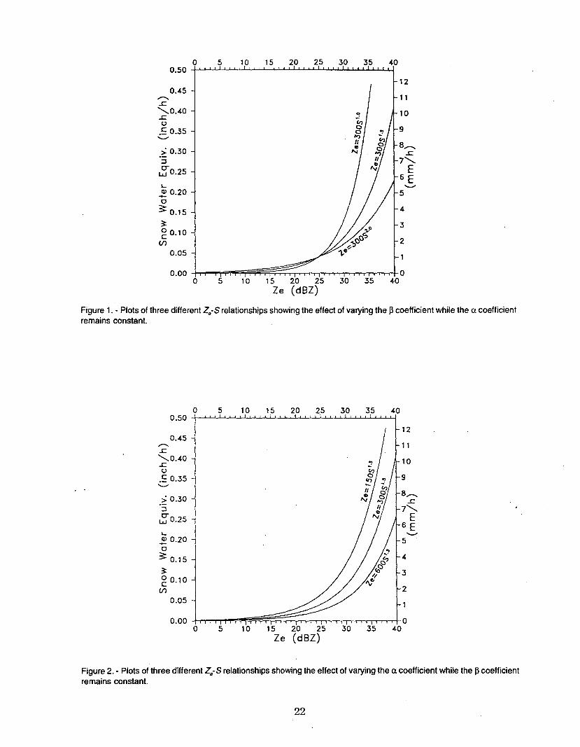
0 5 10 15 20 25 30 35 400.50

120.45

......... 11...r::'-.....0.40 ~10...r::

u.£ 0.35 9...........

> 0.308.........

...r::::J 7'-.....C- E4J 0.25 6EL. ...........Q)

0.20 5-c3: 0.15 4

~I 3g 0.10V) 2

0.05

0.00 00 5 10 15 20 25 30 35 40

Ze (d8Z)

Figure 1. - Plots of three different Ze-S relationships showing the effect of varying the ~coefficientwhile the <Xcoefficient

remains constant.

0 5 10 15 20 25 30 35 400.50 I

120.45

......... 11...r::'-.....0.40 10...r::u

.£ 0.35 9...........

> 0.308.........

...r::::J 7'-.....c- E

~0.251 6E...........

Q) 0.20 5-c3: 0.15 4

~3g 0.10

2t/)

0.05

0.00 00 5 10 15 20 25 30 35 40

Ze (d8Z)

Figure 2. - Plots of three different Ze-S relationships showing the effect of varying the <Xcoefficient while the ~coefficient

remains constant.

22

Fujiyoshi et al. (1990) used 3-minute radar measurements and I-minute sensitiveelectrobalance observations of snowfall intensity only 8.7 km from a 3.2-cm radar. Theyarrived at values of a =427 and ~= 1.09 for the range 0.1 to 3.0 mm h-1 (0.004 to 0.118 inchh-1). Unfortunately, in this generally well-done study, the accuracy of snowfall measurementsis questionable. The authors note that the snowfall amount was 50 percent lower at thewestern end of their line of three measurement sites where the wind "blew harder." Thethree sites were spaced only 100 m apart, and only data from the center site were finallyused. Although a windbreak was used to protect the electrobalance, how this windbreakaffected snowfall onto the balance in the reported 5- to 6-m S-l winds is not clear. As

discussed in section 3.1, wind speeds of that magnitude can cause significant undercatch byshielded gages. The question of snowfall accuracy is not well addressed in numerous studies.

Fujiyoshi et al. (1990) group together values based on both calculations of Z andmeasurements of Ze in their figure 7, which shows published a values for snowfall rangingfrom as low as 50 to almost 4000. Not all the references cited are readily available, but itseems likely that most if not all of the highest values are from studies which calculated Z(e.g., equation (4) is included). But even limiting a values to those based on measured Zewould result in a large range. Values of ~ in the same figure range from 0.9 to 2.3, also aconsiderable range.

Published values of both a and ~vary considerably. Although no unique Z-S relationship canbe expected, what is not clear is how much of the published variation in coefficients is causedby natural differences in snowfall characteristics and how much is related to experimentalshortcomings. Developing the "best" values for a and ~for snowfall in any given geographicalregion is clearly a challenge. And adding to the challenge is the need for large numbers ofdata pairs for calculation as discussed by Krajewski and Smith (1991) (see their fig. 6simulating synchronous observations). Ideally, hundreds of pairs of observations would beused to establish Ze-S relationships, a difficult and expensive undertaking at any singlelocation much less at many geographic regions.

One of the reasons that determining the "best" a and ~coefficients for snowfall is difficult canbe illustrated by figures 1 and 2. . Figure 1 shows the effect of varying the ~value between1.0 and 2.0 while holding the a value constant at 300, all reasonable values according to theliterature. The lower the ~ value, the more rapidly the curve rises with increasing radarreturns. The 3 curves barely deviate for values of Ze lower than the 25-dBZ crossover pointwhere all 3 predict 0.04 inch h-1. As discussed in section 5, most S observations in this studywere below 0.04 inch h-1. Only for Ze values above 30 dBZ do the curves deviate markedlyfrom one another. But this region of relatively high snowfall rates is where data pointsbecome infrequent because of the highly skewed nature of precipitation intensities. So theZe-S relation is relatively insensitive to changes in ~ for the large majority of hours withsnowfall, a point made by Wilson (1975).

On figure 2, the a value of equation (1) is doubled from 150 to 300 and then doubled againto 600, while ~ is left constant at 1.5, again reasonable values according to the literature.Lower a values cause the curves to rise more rapidly as Ze increases. So a rapid rise inpredicted snowfall with increasing Ze can be achieved with either a decrease in a or ~or both.

In the case of figure 2, the curves begin to deviate from one another above 20 dBZ, so thechance of determining the "best" a value may be better than the chance of determining the"best" ~value with typical snowfalls.

23

8. Optimization Scheme for Determination of a and ~Coefficients

An optimization scheme was developed for determining the best a and ~ coefficients forequation (1), repeated below, for any given data set; that is, from the Ze values in an arrayof range bins over a particular gage and simultaneous hourly S observations by that gage.

Z =aSI3e (1)

This scheme is based on the work of Smith et al. (1975) and personal communication withDr. Paul Smith. The approach is discussed in more detail in appendix A by Dr. JamesHeimbach, who programmed the scheme for use with the Cleveland and Denver data sets.

The average estimated snowfall accumulation for each vertical (or upwind) array of9 or morerange bins was repeatedly calculated as described in section 6. At the suggestion of Dr. PaulSmith, for any specified value of ~ in equation (1), a unique value of a was established byforcing the average radar-derived snowfall accumulation to be equal to the average gagehourly snowfall accumulation for each data set (e.g., all pairs of hourly accumulationsobserved by a particular gage and radar estimates over that gage). This constraint simplifiedthe optimization process by limiting the solution to one of a set of ~values, each with onlyone a. A more complex scheme might vary both a and~. Moreover, as pointed out by Smithet al. (1975), the optimization scheme is not restricted to equation (1) because higher orderterm equations could be tested. But the work herein has been limited to equation (1) withthe constraint of using only a unique a value for each ~value.

It is again emphasized that radar estimates of S, not Ze values, were calculated for eachrange bin using equation (1), summed, and averaged in each iteration of this optimizationprocess. This approach avoids the biases resulting from averaging Ze over time and space.

Calculations were made for any input range of ~and ~increment. A CTF (criterion function)was used to judge the fit of each pair of a and~. Smith et al. (1975) discuss the difficultiesof selecting the most appropriate CTF. The CTF used here is the simple sum of absolutedifferences between the gage measurement of precipitation and that estimated by the radar,again as suggested by Dr. Paul Smith. The combination of a and ~ accepted for anyoptimization run was that which yielded the smallest CTF value.

Operator-input values to this scheme include:

. The particular gage to be tested.

. The range of~ and its increment. Unless otherwise stated, the range was from 0.7 to 3.0in steps of 0.05.

. The minimum number of volume scans required for 1 hour of data to be accepted, always.set at 4.

. The minimum number of range bins needed, always set at 5. But in fact, no missingrange bins have been noted so this requirement appears unnecessary.

Range bins commonly had no detectable signal during the beginning and ending portions ofstorms and/or over distant gages. The estimated snowfall rates for all such bins were set to

24

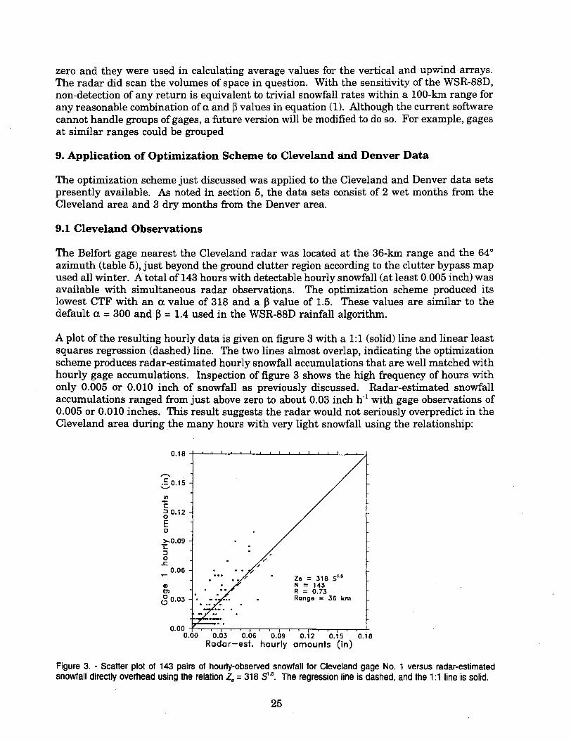
zero and they were used in calculating average values for the vertical and upwind arrays.The radar did scan the volumes of space in question. With the sensitivity of the WSR-88D,non-detection of any return is equivalent to trivial snowfall rates within a 100-km range forany reasonable combination of exand ~values in equation (1). Although the current softwarecannot handle groups of gages, a future version will be modified to do so. For example, gagesat similar ranges could be grouped

9. Application of Optimization Scheme to Cleveland and Denver Data

The optimization scheme just discussed was applied to the Cleveland and Denver data setspresently available. As noted in section 5, the data sets consist of 2 wet months from theCleveland area and 3 dry months from the Denver area.

9.1 Cleveland Observations

The Belfort gage nearest the Cleveland radar was located at the 36-km range and the 64°azimuth (table 5), just beyond the ground clutter region according to the clutter bypass mapused all winter. A total of 143 hours with detectable hourly snowfall (at least 0.005 inch) wasavailable with simultaneous radar observations. The optimization scheme produced itslowest CTF with an exvalue of 318 and a ~ value of 1.5. These values are similar to thedefault ex =300 and ~= 1.4 used in the WSR-88D rainfall algorithm.

A plot of the resulting hourly data is given on figure 3 with a 1:1 (solid) line and linear leastsquares regression (dashed) line. The two lines almost overlap, indicating the optimizationscheme produces radar-estimated hourly snowfall accumulations that are well matched withhourly gage accumulations. Inspection of figure 3 shows the high frequency of hours withonly 0.005 or 0.010 inch of snowfall as previously discussed. Radar-estimated snowfallaccumulations ranged from just above zero to about 0.03 inch h-1with gage observations of0.005 or 0.010 inches. This result suggests the radar would not seriously overpredict in theCleveland area during the many hours with very light snowfall using the relationship:

0.18

'"'.!: 0.15-..;

Ze = 318 5'.5N = 143R = 0.73Range = 36 km

en.....c:

~0.12

Ec

>-.0.09L::J0

.r:::.0.06

0.000.00 0.03 0.06 0.09 0.12 0.15 0.18

Radar-est. hourly amounts (in)

Figure 3. - Scatter plot of 143 pairs of hourly-observed snowfall for Cleveland gage No.1 versus radar-estimatedsnowfall directly overhead uSing the relation Ze = 318 5..5. The regression line is dashed, and the 1:1 line is solid.

25

Distance Beam Standard Error AverageGage from Radar Height* Hours of Estimate SNo. (kIn) (m) Observation a ~R (in h'l) (in h'l)

1 36 390 143 318 1.50 0.73 0.0136 0.01962 61 750 235 248 1.45 0.81 0.0139 0.02043 87 1205 187 147 1.85 0.67 0.0226 0.02604 115 1780 202 48 2.20 0.72 0.0179 0.02325 146 2530 218 8 8.50 0.50 0.0169 0.0196

Z = 318 81.5e

(8)

The best estimates of exand ~should be from gage No.1, nearest the radar. However, theoptimization scheme was applied to all 5 gages east-northeast of Cleveland as summarizedin table 8. Applying the optimi2;ation scheme at more distant ranges provides some insightinto expected underestimation of S by the radar as range increases and the beam becomesbroader and higher above the terrain. At some far range, the radar beam will be above snow-producing clouds, and returns will be negligible even when heavy snowfall is occurring belowthe beam.

Both the "optimum" values of exand ~change with range in table 8. The optimization schemecaused exto decrease and ~to increase with range as the calculations attempted to match theobservations with the constraint that the average radar estimate must equal the average Svalue at each gage. Eventually, absurd values resulted at gage No.5, 146 km from the radar.

Table 8. - Summary of results of applying the optimization scheme to the five gages located east-northeast of Cleveland. Only hours with gage amounts of 0.005 or more inches are included.

* Height of 0.50 tilt beam center above gage assuming standard refraction.

The average hourly S values were consistent along the line of gages, ranging only between0.0196 and 0.0260 inch. Table 7 showed that the median was near 0.01 inch h'l at each gage,and average accumulations varied only between 0.019 and 0.025 inch h-l. The Cleveland lineof gages appears to have produced a reasonably similar data set, providing the opportunityto examine range effects on radar estimates.

A linear least-squares regression line (hereafter regression line), linear correlation coefficient,R, and standard error of estimate were calculated for each gage using the exand ~values oftable 8 and the same data sets to which the optimization scheme was applied. The standarderror of estimate measures the scatter in the Y-direction of the observed points about theregression line and is analogous to the standard deviation. For a large normal distribution,68 percent (95 percent) of the population would fall within plus or minus 1 (2) standard errorof estimate of the regression line. Limited variation of the standard error appears to occurwith range although the two gages closest to the radar have the smallest standard errors.

The R values in table 8 are encouraging. In spite of generally low precipitationaccumulations typical of snowfall, the correlations between the hourly gage observations andradar estimates are generally at least as high as the 0.68 reported by Smith et al. (1975) for

.hourly rainfall on the northern Great Plains. The notable exception is the most distant gageat the 146-km range. No time delay to allow for snowflakes to settle from the illuminatingradar beam to the surface has yet been applied to these data. Neither has the advection

26

Gage Distance A B R Standard Gage RadarNo. from Radar (in) Error Observation Estimation Gagel

(kIn) Estimate (in) (in) (in) Radar

1 36 0.001 0.985 0.73 0.0136 0.0196 0.0196 1.002 61 0.000 1.187 0.80 0.0140 0.0204 0.0173 1.183 87 0.004 1.400 0.68 0.0224 0.0260 0.0160 1.634 115 0.009 1.856 0.72 0.0177 0.0232 0.0074 3.145 146 0.013 1.607 0.55 0.0162 0.0196 0.0043 4.56

scheme discussed in section 11 been applied. The relatively high R values also suggest thatgage measurements were reasonably accurate. More variability might be expected withunshielded gages in windy locations.

It is reasonable to assume that equation (8), derived from the gage nearest the radar, offersthe best available Ze-S relation for the Cleveland area. In order to provide additional insightinto range effects, figures 4 through 7 were prepared by applying equation (8) to each gage'sdata and the vertical array radar data. (The radar array was 3 by 3 range bins for each ofthese gage locations.) A regression line was also calculated for reference as shown by thedashed lines. Gage values that appeared to be outliers on these and all similar plots, andall hourly totals of 0.10 inch h-1 or more, were verified by checking yet again against theoriginal charts.

Table 9 summarizes the results of the various calculations.

Table 9. - Summary of applying equation (8) to the data set from each Cleveland area gage. Alsonoted are the intercept (A) and slope (B) of regression lines (gage =A + B x radar), correlationcoefficients (R), standard error of estimate, average hourly gage-observed and radar-estimated snowfallaccumulations, and the gage/radar estimate ratios. The number of pairs is the same as given intable 8.

Reference to figures 4 through 7 and table 9 shows a number of interesting features. Mostimportant, the gage/radar ratio increases with range as anticipated. The ratios suggest thatradar estimates are 85 percent (111.18) of gage average snowfall by a 61-km range and 61percent by 87 km. Bya 115-to 146-km range, the radar predictions have fallen to only 32 to22 percent of the gage amounts. As shown in table 8, the center height of the 0.5° tilt beamincreases from about 390 m above gage No.1 to over 2500 m above gage No.5, sounderestimates with increasing range should be expected.

Although radar underestimation is serious beyond 60 km, these results are not as drastic asthose reported by Wilson (1975) for a nearby region of the country. Gage:radar ratios wereestimated from the curve on his figure 2 for the ranges of Cleveland gages No.1 to 4. Theseratios, divided by the 36-km ratio, yielded results compatible with table 9 (all of Wilson'sratios exceeded 3.0 because of use of an inappropriate Z-S relation). Resulting values forranges of 61, 87, and 115 km are 1.7, 3.7, and 18.0, much higher than the ratios of table 9.At least three factors probably improve the results given here. The WSR-88D radar beamis narrower (0.95 versus 1.7°) and tilted nearer the ground (0.5 versus 0.9°) than the radarused by Wilson. In addition, the WSR-88D is more sensitive than radars available at thetime of Wilson's study.

27

.........

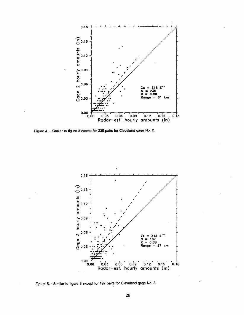
.~ 0.15'-'"

UI0+-r::J 0.120Ec>-0.09

~:J0

.£:0.06

N

CDC'I

~0.03

0.18

//. /

/

l'. //. /.

Ze = 318 s'~N = 235R = 0.80Range = 61 km

0.000.00 0.03 0.06 0.09 0.12 0.15 0.18

Radar-est. hourly amounts (in)

Figure 4. - Similar to figure 3 except for 235 pairs for Cleveland gage No.2.

.........

.= 0.15'-'"

UI0+-r:

~0.12

Ec

>-0.09~:J0

.£:

I") 0.06

CDC'I

~ 0.03

0.18

//

//

//

//. /

//

/. ./.. /. .// .

Ze = 318 s'~N = 187R = 0.68Range = 87 km

0.000.00 0.03 0.06 0.09 0.12 0.15 0.18

Radar-est. hourly amounts (in)

Figure 5. - Similar to figure 3 except for 187 pairs for Cleveland gage No.3.

28

0.18

-i

~O.15

j

l

::J 0.12

E 1

:0.09 {~ ,::J -1

0 J I

r:: I . /

0.06l

: . ! .

"<t . . .. J .

Q) "/..m ":j.

250.03 _7.-..

/

/

/. .. /

./

Ze = 318 S"s

f

N = 202R = 0.72R.09"=

"5~

0.12 0.15 0.18amounts (in)

0.000.00 0:03 0.06 0.09

Radar-est. hourly

Figure 6. - Similar to figure 3 except for 202 pairs for Cleveland gage NO.4.

0.18

i

~0.091

::J

0..c

0.06Ll)

/

//

//

I/

I

/./

/

. :.-/.

/

...-..

.~ 0.15..........

If)

1-C::J0.120

E0

Q)

m

25 0.03

Ze = 318 51.5

N = 218R = 0.55Range = 146 km

~,

l-I

[

0.000.00 0.03 0.06 0.09 0.12 0.15 0.18

Radar-est. hourly amounts (in)

Figure 7. - Similar to figure 3 except for 218 pairs for Cleveland gage No.5.

29

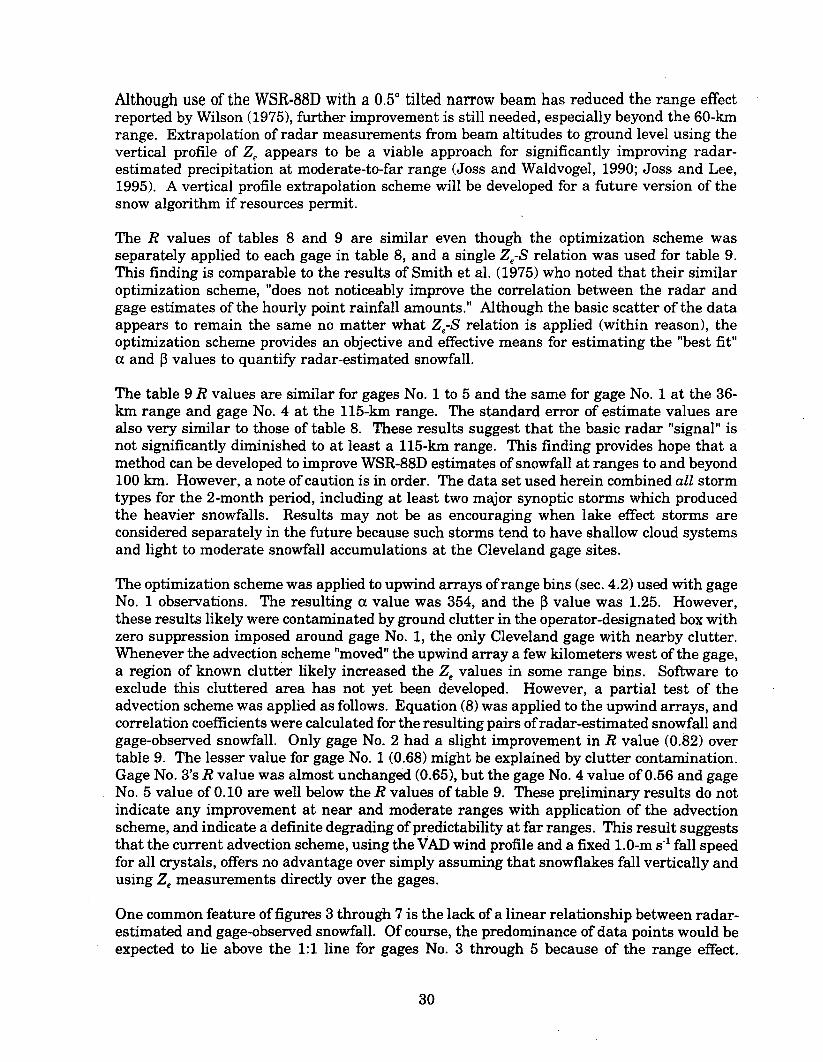
Although use of the WSR-88D with a 0.50 tilted narrow beam has reduced the range effectreported by Wilson (1975), further improvement is still needed, especially beyond the 60-kmrange. Extrapolation of radar measurements from beam altitudes to ground level using thevertical profile of Ze appears to be a viable approach for significantly improving radar-estimated precipitation at moderate-to-far range (Joss and Waldvogel, 1990; Joss and Lee,1995). A vertical profile extrapolation scheme will be developed for a future version of thesnow algorithm if resources permit.

The R values of tables 8 and 9 are similar even though the optimization scheme wasseparately applied to each gage in table 8, and a single Ze-S relation was used for table 9.This finding is comparable to the results of Smith et al. (1975) who noted that their similaroptimization scheme, "does not noticeably improve the correlation between the radar andgage estimates of the hourly point rainfall amounts." Although the basic scatter of the dataappears to remain the same no matter what Ze-S relation is applied (within reason), theoptimization scheme provides an objective and effective means for estimating the "best fit"a and ~values to quantify radar-estimated snowfall.

The table 9 R values are similar for gages No.1 to 5 and the same for gage No.1 at the 36-km range and gage No.4 at the U5-km range. The standard error of estimate values arealso very similar to those of table 8. These results suggest that the basic radar "signal" isnot significantly diminished to at least a U5-km range. This finding provides hope that amethod can be developed to improve WSR-88D estimates of snowfall at ranges to and beyond100 km. However, a note of caution is in order. The data set used herein combined all stormtypes for the 2-month period, including at least two major synoptic storms which producedthe heavier snowfalls. Results may not be as encouraging when lake effect storms areconsidered separately in the future because such storms tend to have shallow cloud systemsand light to moderate snowfall accumulations at the Cleveland gage sites.

The optimization scheme was applied to upwind arrays of range bins (sec. 4.2) used with gageNo.1 observations. The resulting a value was 354, and the ~ value was 1.25. However,these results likely were contaminated by ground clutter in the operator-designated box withzero suppression imposed around gage No.1, the only Cleveland gage with nearby clutter.Whenever the advection scheme "moved" the upwind array a few kilometers west of the gage,a region of known clutter likely increased the Ze values in some range bins. Software toexclude this cluttered area has not yet been developed. However, a partial test of theadvection scheme was applied as follows. Equation (8) was applied to the upwind arrays, andcorrelation coefficients were calculated for the resulting pairs of radar-estimated snowfall andgage-observed snowfall. Only gage No.2 had a slight improvement in R value (0.82) overtable 9. The lesser value for gage No.1 (0.68) might be explained by clutter contamination.Gage No. 3's R value was almost unchanged (0.65), but the gage No.4 value of 0.56 and gageNo.5 value of 0.10 are well below theR values of table 9. These preliminary results do notindicate any improvement at near and moderate ranges with application of the advectionscheme, and indicate a definite degrading of predictability at far ranges. This result suggeststhat the current advection scheme, using the VAD wind profile and a fixed 1.0-m S-1fall speedfor all crystals, offers no advantage over simply assuming that snowflakes fall vertically andusing Ze measurements directly over the gages.

One common feature offigures 3 through 7 is the lack of a linear relationship between radar-estimated and gage-observed snowfall. Of course, the predominance of data points would beexpected to lie above the 1:1 line for gages No.3 through 5 because of the range effect.

30

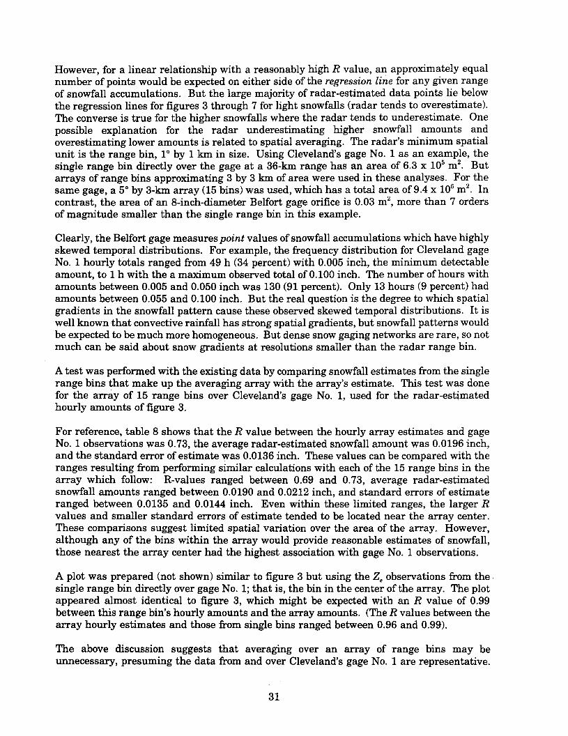
However, for a linear relationship with a reasonably high R value, an approximately equalnumber of points would be expected on either side of the regression line for any given rangeof snowfall accumulations. But the large majority of radar-estimated data points lie belowthe regression lines for figures 3 through 7 for light snowfalls (radar tends to overestimate).The converse is true for the higher snowfalls where the radar tends to underestimate. Onepossible explanation for the radar underestimating higher snowfall amounts andoverestimating lower amounts is related to spatial averaging. The radar's minimum spatialunit is the range bin, 10 by 1 km in size. Using Cleveland's gage No.1 as an example, thesingle range bin directly over the gage at a 36-km range has an area of 6.3 x 105 m2. Butarrays of range bins approximating 3 by 3 km of area were used in these analyses. For thesame gage, a 50 by 3-km array (15 bins) was used, which has a total area of 9.4 x 106m2. Incontrast, the area of an 8-inch-diameter Belfort gage orifice is 0.03 m2, more than 7 ordersof magnitude smaller than the single range bin in this example.

Clearly, the Belfort gage measures point values of snowfall accumulations which have highlyskewed temporal distributions. For example, the frequency distribution for Cleveland gageNo.1 hourly totals ranged from 49 h (34 percent) with 0.005 inch, the minimum detectableamount, to 1 h with the a maximum observed total of 0.100 inch. The number of hours withamounts between 0.005 and 0.050 inch was 130 (91 percent). Only 13 hours (9 percent) hadamounts between 0.055 and 0.100 inch. But the real question is the degree to which spatialgradients in the snowfall pattern cause these observed skewed temporal distributions. It iswell known that convective rainfall has strong spatial gradients, but snowfall patterns wouldbe expected to be much more homogeneous. But dense snow gaging networks are rare, so notmuch can be said about snow gradients at resolutions smaller than the radar range bin.

A test was performed with the existing data by comparing snowfall estimates from the singlerange bins that make up the averaging array with the array's estimate. This test was donefor the array of 15 range bins over Cleveland's gage No.1, used for the radar-estimatedhourly amounts of figure 3.

For reference, table 8 shows that the R value between the hourly array estimates and gageNo.1 observations was 0.73, the average radar-estimated snowfall amount was 0.0196 inch,and the standard error of estimate was 0.0136 inch. These values can be compared with theranges resulting from performing similar calculations with each of the 15 range bins in thearray which follow: R-values ranged between 0.69 and 0.73, average radar-estimatedsnowfall amounts ranged between 0.0190 and 0.0212 inch, and standard errors of estimateranged between 0.0135 and 0.0144 inch. Even within these limited ranges, the larger Rvalues and smaller standard errors of estimate tended to be located near the array center.These comparisons suggest limited spatial variation over the area of the array. However,although any of the bins within the array would provide reasonable estimates of snowfall,those nearest the array center had the highest association with gage No.1 observations.

A plot was prepared (not shown) similar to figure 3 but using the Ze observations from the.single range bin directly over gage No.1; that is, the bin in the center of the array. The plotappeared almost identical to figure 3, which might be expected with an R value of 0.99between this range bin's hourly amounts and the array amounts. (The R values between thearray hourly estimates and those from single bins ranged between 0.96 and 0.99).

The above discussion suggests that averaging over an array of range bins may beunnecessary, presuming the data from and over Cleveland's gage No.1 are representative.

31

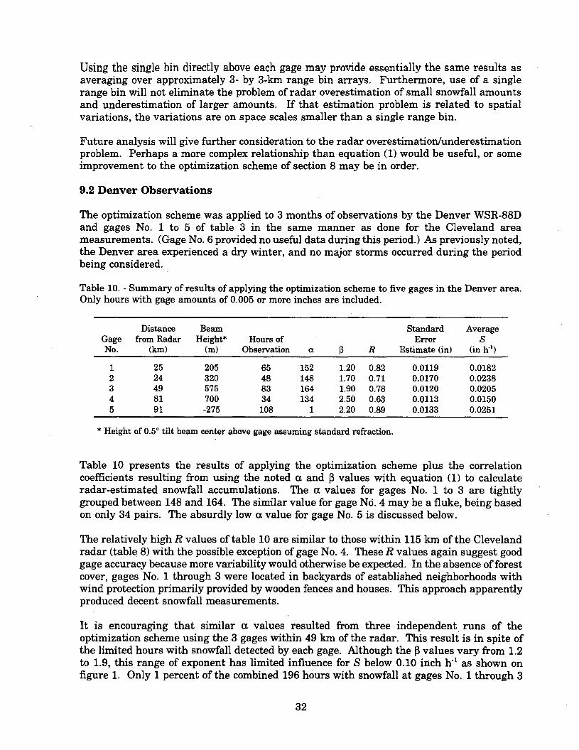
Distance Beam Standard AverageGage from Radar Height* Hours of Error SNo. (km) (m) Observation a ~R Estimate (in) (in h-1)

1 25 205 65 152 1.20 0.82 0.0119 0.01822 24 320 48 148 1.70 0.71 0.0170 0.02383 49 575 83 164 1.90 0.78 0.0120 0.02054 81 700 34 134 2.50 0.63 0.0113 0.01505 91 -275 108 1 2.20 0.89 0.0133 0.0251

Using the single bin directly above each gage may provide essentially the same results asaveraging over approximately 3- by 3-km range bin arrays. Furthermore, use of a singlerange bin will not eliminate the problem of radar overestimation of small snowfall amountsand underestimation of larger amounts. If that estimation problem is related to spatialvariations, the variations are on space scales smaller than a single range bin.

Future analysis will give further consideration to the radar overestimation/underestimationproblem. Perhaps a more complex relationship than equation (1) would be useful, or someimprovement to the optimization scheme of section 8 may be in order.

9.2 Denver Observations

The optimization scheme was applied to 3 months of observations by the Denver WSR-88Dand gages No.1 to 5 of table 3 in the same manner as done for the Cleveland areameasurements. (Gage No.6 provided no useful data during this period.) As previously noted,the Denver area experienced a dry winter, and no major storms occurred during the periodbeing considered.

Table 10. - Summary of results of applying the optimization scheme to five gages in the Denver area.Only hours with gage amounts of 0.005 or more inches are included.

* Height of 0.50 tilt beam center above gage assuming standard refraction.

Table 10 presents the results of applying the optimization scheme plus the correlationcoefficients resulting from using the noted ex and ~ values with equation (1) to calculateradar-estimated snowfall accumulations. The ex values for gages No.1 to 3 are tightlygrouped between 148 and 164. The similar value for gage No.4 may be a fluke, being basedon only 34 pairs. The absurdly low exvalue for gage No.5 is discussed below.

The relatively high R values of table 10 are similar to those within 115 km of the Clevelandradar (table 8) with the possible exception of gage No.4. These R values again suggest goodgage accuracy because more variability would otherwise be expected. In the absence offorestcover, gages No.1 through 3 were located in backyards of established neighborhoods withwind protection primarily provided by wooden fences and houses. This approach apparentlyproduced decent snowfall measurements.

It is encouraging that similar ex values resulted from three independent runs of theoptimization scheme using the 3 gages within 49 kmofthe radar. This result is in spite ofthe limited hours with snowfall detected by each gage. Although the ~values vary from 1.2to 1.9, this range of exponent has limited influence for S below 0.10 inch h-1 as shown onfigure 1. Only 1 percent of the combined 196 hours with snowfall at gages No.1 through 3

32

exceeded this value. The suggestion of table 10 is that the a coefficient for the Denver areashould be about half that of the Cleveland value of318, but the exponents should be similar,near 1.5. Of course, this preliminary conclusion is based on limited data without heavysnowfalls.

The optimization scheme softw~re cannot presently handle input data from more than onegage with its corresponding radar observations. However, it was decided to apply the schemeto gages No.1 and 2 at 24- and 25-km ranges using their average a and f3values from table10; that is, 150 and 1.45, respectively. The resulting radar estimates and gage observationswere then grouped together to increase the population to 113 pairs. The resulting R valuewas a respectable 0.76 and the regression line essentially matched the 1:1 line. The averagea =150 and f3=1.45 were used with equation (1) to estimate snowfall with the vertical arrayover gage No.3, which resulted in an average radar-estimated snowfall of 0.0211 inch h-\slightly above the value of table 10. The corresponding R value was 0.79. These resultsindicate no significant decrease in radar estimation to at least a 49-km range; that is, norange effect.

With the absence of any discernible range effect out to at least gage No.3, the average a andf3values for gages No.1 to 3 of table 10 were used in equation (9) to estimate snowfallaccumulations from the vertical arrays over gages No.1 to 3.

Z = 155 81.6e

(9)

The resulting 196 data pairs are plotted on figure 8 along with the regression line, whichalmost matches the 1:1 line. The correlation coefficient is 0.76. The average radar-estimatedand gage-observed hourly snowfall proved to be identical at 0.0205 inch. These resultssuggest that equation (9) is a good first approximation to use with winter storms in theDenver area. But as with the similar Cleveland area figures, a marked tendency is seen onfigure 8 for the radar estimates to be too high for .low snowfalls and too low for higherobserved accumulations.

Little can be said about gage No.4 observations with only 34 hours of detectable snowfall ata low average value of 0.015 inch. This broad mountain valley site was chosen because itwas surrounded by mountains but had no ground clutter for several kilometers around it.This location seemed to offer a good opportunity to evaluate mountain valley sites wherepeople tend to live. However, it has become apparent that the location is in a distinct "rain(and snow) shadow" because of downslope motion from higher terrain.

Gage No.5 was deliberately chosen as a mountain site in the midst of a very cluttered areaaccording to the clutter bypass map used by the Denver WSR-88D all winter. Its data canbe used to evaluate whether the Denver radar might be used to estimate snowfall over theRocky Mountains. Examination of PPI radar displays from Depver generally reveals a largearea with very little reflectivity from low tilts over the Rocky Mountains because of beamblockage and clutter suppression. The altitude of gage No.5 is above the center of the 0.50beam (for standard refraction), the only reflectivity data so far examined, and little usefulinformation was expected from this lowest tilt beam. Future plans include examination ofradar returns from higher tilts.

33

0.12

.........c:

'-" 0.10en.....c:::J0E 0.080

>-~ 0.060

..c:

toI 0.04 Ze = 155 S'.6

N = 196R = 0.76Ranges: 24-49 km

enQ)rnO.020

<.:>

0.000.00 0.02 0.04 0.06 0.08 0.10 0.12

Radar-est. hourly amounts (in)

Figure 8. - Scatter plot of 196 pairs of hourly-observed snowfall for Denver gages No.1 to 3 versus radar-estimatedsnowfall directly overhead using the relation Ze = 155 51.6. The regression line is dashed. and the 1:1 line is solid.

The R value for gage No.5 is the highest in table 10 and the a value is extremely low at 1.0.Table 10 shows that the center of the 0.50 tilted beam was below the elevation of gage No.5, so ground clutter and beam blockage would certainly be expected near this gage. The 9range bins in the vertical array over gage No.5 were briefly inspected for many volumescans. Range bins along about the 260 and 261 0 radials for ranges of 90 to 92 km rarely hadany detectable returns. Such bins were assumed to represent zero snowfall in the processingsoftware. However, the 3 bins along the 2620 radial frequently had returns, albeit withrelatively low Ze values. The RDRHGT program discussed in section 3.3 shows almost totalblockage of the 0.50 beam near gage No.5 for the 260 and 2610 radials, and a large fractionof the beam is unblocked for the 2620 radial.

Because the snowfall rate was calculated for each bin in an array and then averaged, theusual inclusion of about 6 zero values over gage No.5 resulted in very low snowfall estimates.The optimization scheme, in forcing radar estimates and gage observations to have the sameaverage values, produced the very Iowa value and relatively high f3 value. A plot of theresulting radar estimates and gage measurements (not shown) shows limited scatter, inagreement with the R value of 0.89. But when the reasonable a. and f3values of equation (9)were used, most radar-estimated hourly snowfalls became trivial. .

The 3 range bins along the 2620 radial over gage No.5 contained enough signal to give riseto some optimism. These results suggest that radar returns that are not totally blocked orsuppressed may be used over mountainous terrain to provide some estimates of snowfallintensity. Further work is warranted on the topic of radar estimation of snowfall onmountainous terrain, including consideration of the 1.50 beam.

Upwind arrays were also used with gages No.1 to 5 in the optimization scheme. Some Rvalues increased slightly, but no more than 0.02 over those values in table 10. These resultssuggest the current advection scheme offers no significant increase in predictive value in theDenver area over simply using the range bins directly above the location of interest.

34

Finally, equation (9) was applied to all five gages with the result that the R values werebasically unchanged from table 10, similar to the Cleveland findings, with the exception ofgage No.5 which had its R value reduced from 0.89 to 0.82. Moreover, the radar-estimatedsnowfall accumulations were reasonable except at gage No.5. The average radar-estimatedhourly snowfall accumulation over gage No.5 was 0.002 inch, and the gage-observed valuewas 0.025 inch h-1. So, with the exception of the blocked and cluttered mountainous regions,use of equation (9) appears justified in the Denver area, at least until testing with additionaldata is possible.

9.3 Significance of Different Ze-S Relations for Cleveland and Denver

The recommended initial exand ~values are 318 and 1.5 for Cleveland and 155 and 1.6 forDenver. These values are very similar to the top two curves of figure 2.

It is reasonable to ask whether these curves produce sufficiently different snowfallaccumulations to make a practical difference. One way to address that question is to applythe Cleveland relation of equation (8) to Denver data and the Denver relation of equation (9)to Cleveland data. This application produced the results shown on figures 9 and 10,respectively.

Examination of figure 9 reveals Cleveland equation (8) significantly underpredicts Denverhourly snowfall accumulations. The dashed regression line is well above the 1:1 line, and theaverage radar-estimated snowfall accumulation is 0.0126 inch, 61 percent of the gage-observed 0.0205 inch. Conversely, figure 10 shows use of Denver equation (9) with Clevelandradar measurements seriously overpredicts snowfall accumulations as shown by theregression line well below the 1:1 line. The average radar-estimated snowfall accumulationin this case is 0.0289 inch, 144 percent of the gage-observed average value of 0.0201 inch.Use of a Ze-S relationship appropriate to the geographical region clearly is important forquantitative snowfall estimation.

It is not known why the different Ze-S relations resulted from the Cleveland and Denver areadata. The difference may be related to microphysical differences between the lake effectstorms that predominated over the Cleveland gages and the upslope storms that affected the.Denver area. Ice crystal observations were routinely made near Denver but not nearCleveland. However, microphysical observations of lake effect storms have been publishedwhich may be compared with the past winter's Denver observations in a future report.

35

0.12

//

i/

/

"20.10

'-"(I)

C 0.08:J0E00.06>-L:J0

L 0.04

.'//

/., , ,.,

/ 'DEN gages 1-3

Ze = 318 51.5

N = 196R = 0.76Ranges: 24-49 km

. .- .,...Q)

rn0

<.:>0.02

I I I . I0.02 0.04 0.06 0.08 0.10

Radar-est. hourly amounts (in)

Figure 9. - Similar to figure 8 except the Cleveland Ze-S relationship of figure 3 is deliberately misapplied to Denvergages No.1 to 3.

0.000.00

ILI

ii

0.12

O. 14

1

-~E gages '1-2

Ze = 155 51.6. N = 378 .

.~ 0.12 R = 0.77'-" Ranges: 36-61 km

~ 1s:: 0.10 -;:J ;

0 -j

E I0 0.08 l~ 0.06

1

0L

Q)0.04

rn0

<.:>0.02

/. /

//

//

//- . ./,

/',/

'

~

,- --, - . ,/.-. 7-.. - ./'.. -- - ..

-- . ..0.000.00 0.02 0.04 0.06 0.08 0.10 0.12 0.14

Radar-est. hourly amounts (in)

Figure 10. - Similar to figure 9 except that the Denver Ze-S relationship of figure 8 is deliberately misapplied toCleveland gages NO.1 and 2.

36

10. Development of a Snow Accumulation Algorithm for the NEXRAD RadarSystem, First Version: June 1996

10.1 Introduction

The MOD specifies several milestones for the delivery of results in the development of theSnow Accumulation Algorithm (hereafter Snow Algorithm) for the NEXRAD radar system.The following sections and appendices describe the Snow Algorithm itself and not theassociated data gathering activities (secs. 2 to 6), or their results in specifying a relationshipbetween effective reflectivity factor (Ze) and snow water equivalent (8) on the ground (secs.7 to 9). The appendixes give specific details for the various specialists who will be involvedin the further programming or use of the Snow Algorithm.

. Appendix B contains appendix B of the MOD: Algorithm Documentation Requirements.It specifies a document containing nine sections:

1. Source.2. Bibliography3. Functional Description4. Functional Comparison5. Statistical Performance6. Operational Performance7. Adaptable Parameters8. Strengths and Limitations9. Future Enhancements

However, this report has a different structure. The rest of appendix B identifies thesections of this report that fulfill those requirements.

. Appendix C is the same as appendix C of the MOD: Criteria for Acceptance ofDeliverables. It specifies numerous characteristics to be included in the Snow Algorithm..

. Appendix D summarizes the tasks specified in the SOW given in the MOD and gives thedelivery timetable and preliminary results.

10.2 Relationship to Other OSF Software Programs

This Snow Algorithm is partly based on procedures already in use with the NEXRAD system,specifically the PPS (precipitation processing subsystem), intended for rain, and Dopplerwinds (VAD) portions. Where appropriate, the same PPS or VAD subroutine names havebeen used where they are identical or accomplish the same thing. Likewise, a few of thevariables are the same. The program structure differs in that it does not use the sameshared memory as the PPS and VAD routines because of the complicated addresses in thoseroutines and the reduced program memory space in the development versions. The enclosedsimpler program structure is expected to be rewritten into the NEXRAD software style.

The programs use reflectivity (Ze) data from Level II tapes consisting of dBZ, offset,multiplied by 2, and offset again to yield integer numbers called "biased dBZ" in the PPSsoftware ranging from 0 to 255; 0 indicates that Ze is below the detection level for the WSR-88D. Velocity data are also rescaled to a range of 0 to 255. Resulting numbers are thereforenot "biased" in the normal dictionary sense but are resealed into the byte range of numbers.

37

10.2.1 The PPS Algorithm

The PPS algorithm is described in section 3.3 of the Federal Meteorological Handbook No.11 (1991), Doppler Radar Meteorological Observations, part C, WSR-88D Products andAlgorithms. The algorithm produces maps of accumulated precipitation (intended for rain,not snow) for I-hour, 3-hour, and storm totals. Five basic steps are listed: 1) preprocessing,2) rate, 3) accumulation, 4) adjustment, and 5) products.

1) Preprocessing:

The preprocessing algorithm prepares Ze data for input into the rate algorithm. Qualitycontrol steps include: blockage correction, isolated bin check, outlier check, vertical echocontinuity check, and bi-scan maximization. The beam blockage correction adds 1, 2, 3, or4 dBZ (or 2, 4,6, or 8 to the biased dBZ) to radial data beyond ranges at which the beam isestimated to be blocked by particular percentages. The occultation file has azimuthresolution of 0.20 and is calculated from terrain data specific to each radar antenna site.Isolated bin values of reflectivity are set to a code for "less than minimum detectable signal."Bins with unreasonably large reflectivities are set to a near-minimum level or else to theaverage of the eight adjacent bins. Bins that are completely occulted (>60-percent blockage)are sometimes replaced by the values of adjacent bins having less blockage. An attempt ismade to remove spurious echoes in the lowest tilt ("tilt test") if such echoes tend to disappearin the second tilt. A hybrid-sector file then specifies which tilt to use for precipitationcalculations. At far range, it is one of the two lowest tilts giving the greatest echo (bi-scanmaximization). The reflectivities are then ready for those further calculations.

The Snow Algorithm, presented here, uses a new hybrid-sector file, developed by TimO'Bannon of the OSF, which attempts to keep the bottom of the beam closer to the terrainthan previous versions while still maintaining 500 feet vertical separation. It does not yetattempt to use adjacent bins for substitution for beam blockages. It does not use the tilt testbecause snow may occur from shallow clouds that are observed only in the lowest tilt at farrange. Though the preprocessing software coding in this version of the Snow Algorithm hasdifferences in style from that in the PPS version, most of the existing PPS routines areacceptable for snow estimation.

Five significant differences are needed for work with snow:

(a) All radials with data, including overlaps, are stored in an array along with theirprecise azimuth angles. (Each tilt of a volume scan typically has 367 radials of data,including the overlap of the start and end of each tilt. The Snow Algorithm allows upto 370.) No radials are averaged together when their integerized azimuth angles arethe same. Such averaging requires the conversion of reflectivities to precipitationrates before averaging. The integerization of azimuths may leave some angles withno data even though no break occurred in the scan. Instead, a "nearest neighbor"routine is used later when data for a particular azimuth angle are needed. Thatroutine avoids both averaging and gaps.

(b) Reflectivity values are kept in units of biased dBZ rather than precipitation rate. Theconversion back and forth between units adversely quantizes reflectivities at the lowprecipitation rates typical of snow. Averaging of radials is no longer needed in theSnow Algorithm preprocessing. The only other PPS preprocessing averaging is to

38

replace outliers by the simple average of its eight neighbors. The Snow Algorithmdoes the conversion back and forth only for those neighbors in order to replace onlythe outlier itself; as in the PPS version, the neighbors are not affected.

(c) The new hybrid scan file is used to keep the bottom of the beam close to, but at least500 feet above, the terrain.

(d) The tilt test is not done because snow may be falling from shallow clouds illuminatedonly by the 0.5° tilt beam at far ranges.

(e) The biscan maximization for the two lowest tilts is not done. Instead, the lowestacceptable tilt is used as a partial protection against virga.

2) Rate:

The PPS uses only a Z-R relation for rain. The constants for the relation are stored in anadaptable parameters file. This Snow Algorithm has found different constants for snow thatdepend on geographic (climate) region. The observed range dependency for snow has not yetbeen addressed.

3) Accumulation:

The PPS sums rainfall for 1° by 2-km sample volumes and also for 1/4 LFM (limited finemesh) grid boxes. Accumulations are made by I-hour, 3-hour, and storm total intervals. Thisversion of the Snow Algorithm sums snowfall in polar coordinate arrays (230 km x 360°) atthe basic resolution of 1° by 1 km. They may be resampled into any other grid style. Theaccumulation grids presently used by the PPS are entirely acceptable for snow. The threetime periods for accumulations are the same as in the PPS version. The Snow Algorithmdoes not yet contain the continuity and quality checks done by the PPS version, but nochanges are anticipated.

4) Adjustment:

The PPS algorithm contail)s coding to compare radar-derived accumulations with those fromprecipitation gages. No such adjustments are yet included in the Snow Algorithm.

5) Products:

The PPS algorithm produces 2- by 2-km grids of rainfall totals at I-hour, 3-hour, and stormtotal intervals. The accumulations from the Snow Algorithm can be transformed to the samegrids that are presently in use.

10.2.2 The VAD Algorithm

The VAD algorithm is described in section 3.11 in part C of Federal Meteorological HandbookNo. 11 (1991) and in chapter 6 of part B of the Handbook. Upper winds are needed at 1000-foot increments above sea level. A range, default 30 km, is assigned for data gatheringpurposes. For each 1000-foot level, the range at which each tilt's beam crosses that level iscalculated. The tilt yielding the closest range to the 30 km is then used. All valid velocitymeasurements at that tilt and range are fitted to a sine wave as a function of azimuth. The

39

phase of the sine wave gives the azimuth of the winds. The amplitude of the sine wave,divided by the cosine of the tilt, gives the horizontal wind speed. The fitting is done insuccessive iterations; outlier values are discarded between iterations.

The Snow Algorithm uses nearly,the same processes for determining the vertical wind profileand the same VAD subroutines for the fitting itself. The first difference, apart from codingstyle, is that more data points are used. Four velocity measurements reside within eachreflectivity bin of 1-km length. The Snow.Algorithm uses the velocity measurements within0.5 km of the calculated range. That distance increases the data density for the fittingroutine and should thereby improve the fit. Secondly, the 30-km nominal range has beenchanged to 10 km, a value used by some radar sites. The radar beam is therefore smallerwhen it passes through each 1000-foot interval. Comparing the 10-km with the 30-km resultsshows that the latter are systematically biased toward greater speeds. The top of the beamnormally samples greater speeds than the bottom under typical wind profiles. The tallerbeam at 30 km sees a greater spread of velocities than the shorter beam at 10 km. It is

.

therefore expected that the 10-km wind profiles are more accurate for use in the advectionscheme of the Snow Algorithm. The wind profile is not used in the PPS algorithm for rainbecause rain is not advected as severely as snow.

11. Functional Description of the Snow Algorithm

The Snow Algorithm, RADAR7.F (seventh in a series of development programs), performs thecalculations for the algorithms leading to the integration of snowfall, based on radarreflectivities and wind velocities. The geometry of the Snow Algorithm is nested cylindricalcoordinates. For each tilt (elevation angle), the view is 230 km by 3600 in 1 km and 10resolution for most data. The Algorithm was adapted to a Sun (Solaris 2.4) UNIXenvironment. Rather than use the complexities of the PPS shared memory, this versionmakes use of direct access files. This usage generally affects only coding style and executionspeed but not the functioning of the Snow Algorithm. The Snow Algorithm retains a sharedmemory, /STORE/, for the data used most frequently in the VAD wind and reflectivitycalculations. The Snow Algorithm will be rewritten to conform with NEXRAD programstandards. The Snow Algorithm is' in modules, some of which are very much like thosealready in use in the PPS algorithm and with similar names. Others can be readilyconverted. An abundance of internal comments have been placed in the FORTRAN code sothat programmers can understand what the Snow Algorithm is doing.

Three terrain-based files are needed that are site-specific. The programs generating thesefiles are described in appendix E. The programs themselves are listed in appendixes F, G,and H. The first program simply trims the occultation file of its first four bytes and all of itstrailing bytes in order to create a file that is easy to read by direct access. The secondprogram takes the new hybrid sector file, which is an attempt to have the bottom of the radarbeam be at least 500 ft above the terrain, and greatly rearranges its structure. The resultis a simple direct access file that indicates which elevation tilt is to be used for eachazimuth/range location. The third program generates a file in radar coordinates indicatingthe ground elevation in meters. That terrain file is needed in the advection routine to helpdetermine where falling snow should land on the ground.

40

11.1 General Functions and Subroutines

NCLOCK, ICLOCK, HHMMSS, DATEJ are time and date conversion conveniences. SIND,COSD, and TAND are trigonometric functions using inputs in degrees (°) rather than radians.

BEAMHT(R,E,A) calculates the height of the center of the radar beam at input radius R(km), elevation angle E (degrees), and antenna altitude A (km). The formula uses a 4/3 earthradius relationship. Setting A=O, gives radar beam height 'above the radar antenna.

The following is a "tree" showing, by indentations, which program units call the others.GETRADAR is called by three program units, twice by the main program; the data that aresubsequently used are different with each call. The above program units in the "tree" areomitted. Program units with names starting with "A31" are equivalents to PPS and VADroutines of the same names. The specific differences in each unit between this SnowAlgorithm and those provided by the OSF are listed in appendix J.

PROGRAM. RADAR7A3133D

A3133FGETRADARGETPROF

GETRADARA317G2

A317H2A317I2A317J2A317K2

GETRADARGETARI

GETRADAROCCULTNOSPIKESPRECIP

ADVECTFILENAME

! The main program that calls the other units! _IN IT_ADAPT loads the adaptable parameters! _FILL_PRECIP_TABLE biased dBZ to mm/h * 100! The unpacker of Level II data: header! Calculates the vertical wind profile to 15k ft! The unpacker of Level II data: (dBZ and velocity)! _VAD_PROC! _V AD_LSF! _VAD_RMS! _FIT_TEST! _SYM_CHK! The unpacker of Level II data: header! Loads azimuth-range arrays! The unpacker of Level II data: dBZ (and velocity)! Performs occultation adjustment! Cleans reflectivities of isolateds and outliers! Integrates snowfall rates for both falling styles! Calculates volume scan bins for advected snow! Increments input file name

11.2 Program Unit Description for the Snow Algorithm

GETRADAR:

The IRADIAU list has indices such that an index of 0 indicates a location centered at therange of the radar antenna itself. The subroutine loads all data for each radial into twonamed commons whether they are ever used or not. The /CLOCK/ list has all of the datesand times in "yymmdd" and "hhmmss" format. The VAL array has floating point numbersand the NUM has integer numbers for what might be considered housekeeping numbers:VAL(2), the center azimuth angle; VAL(3), the center elevation angle; NUM(7), the radialstatus; and NUM(8), the RDA elevation number, are used extensively by the rest of the SnowAlgorithm. The other arrays present the reflectivities, velocities, and spectrum widths in

41

both raw and decoded format. The menu in the comment section identifies all variables inthe named common lists. This style of having an unpacker of Level II data that loads thenamed common arrays with full radial data for each call is very convenient. It only takes aCALL GETRADAR to get whatever one might want to know about the next radial's data.

PROGRAM RADAR7

After initiating the adaptable parameters, the Snow Algorithm calls up three files specific tothe sites being considered. The terrain file was generated by "nearest neighbor" samplingfrom 30-arc-second data prepared by the Defense Mapping Agency, which has an originalresolution near 1 km, similar to the radar resolution. A file could be prepared from similar3-arc-second data if greater precision is desired, but that task is not a part of the workdescribed here. The occultation file is the same as that used in the PPS Algorithm exceptthat the first four bytes and all trailing bytes have been stripped to make a file that is easyto examine under direct access. The hybrid scan file is related to that produced by TimO'Bannon for having the bottom of the beam near the terrain but at least 500 feet above it.The expanded sector portion is being ignored; this version of the Snow Algorithm does nottry to substitute for reflectivity data in range bins at the edges of cluttered regions. Theremaining hybrid sector data for the four lowest tilts were merged into one 230- by 360-arraywith numbers 1,2,3, and 4 indicating which tilt (0.5, 1.5, 2.5, or 3.5°) to use for each rangebin. All three site files (terrain, occultation, hybrid scan) are then easily examined by directaccess when needed, avoiding the need to reserve program memory for their full arrays.

The Snow Algorithm uses a file name convention that expects an increment of the file nameextension from 2 to 401, representing the file numbers on a Level II tape that are found afterthe header file. The Snow Algorithm expects a set of files available on a removable or fixedhard disk. The Snow Algorithm calls each file in sequence until the series has no more filesleft. The algorithm then asks for a new file name for a continuation of the processing. Theoperator can thereby step over a gap in the series or insert a different removable disk orLevel II tape when the next expected file is not found. The rewrite of the Snow Algorithmcan use whatever scheme is convenient for obtaining the next file of the series.

After loading and initializing adaptable parameters and site-specific files, the Snow.Algorithm first calculates the vertical wind profile, needed for the advection scheme. TheSnow Algorithm operates basically the same as the current version used by all WSR-88Ds.The software modifications are merely a condensation by removing white space and trivialcomment lines and a substitution of numbers for named constants so that a reader mightbetter understand the processes. The functional modifications allow 4 velocity measurementsper radial rather than 1 and use 10 km rather than 30 km for the default range.

The Level II tape data file on disk is then rewound. The entire file must be checked todetermine the wind profile and the ending time for the scan, all before considering thereflectivities. Both the wind data and the reflectivity data occupy the same /STORE/ namedcommon and therefore must be loaded sequentially. The process could probably be speededup in the rewritten version that does not have memory limits by loading the four reflectivityarrays while the wind data are being examined. That procedure would prevent the necessityfor a rewind and a rereading could be avoided.

The Snow Algorithm then calls GETARI to load the reflectivity arrays. Notice that thedimensions are to 370°, of which 367 are typically needed. Unlike the PPS version, this Snow

42

Algorithm does not average two radials that happen to have the same integerized azimuthangle. Instead, it keeps track of the exact azimuth angles in an array and scans the arrayeach time a particular azimuth is needed. The nearest azimuth to the nominated azimuthis selected. That technique produces no gaps in coverage as can happen with simpleintegerized azimuth angles. The range has been limited to 115 km for the 2.50 tilt and to 10km for the 3.50 tilt. The ranges needed for those tilts for the three sites (Denver, Cleveland,Albany) are within those values according to the expanded hybrid sector files. That rangelimitation saves memory space in the computer environment. It does not affect any results.

The reflectivity storage arrays are in named common rather than in a direct access file. Theadvection scheme needs rapid access to the stored data in almost a random access fashion.Reserving space in named common makes the search go faster than disk access. The SnowAlgorithm differs from the PPS algorithm by saving the biased reflectivity numbers (byte or[*2) rather than floating point dBZ's or precipitation rates. Converting all of the reflectivitiesto precipitation rates before the rest of the manipulations takes time, and converting themall back takes additional time. Furthermore, the RATE_TABLE has the same precipitationrate for a variety of reflectivities. If nothing is ever done to a range bin's reflectivity(averaging, occultation boost), the conversion from biased reflectivity to precipitation rate andback to biased reflectivity almost always results in a different number for weak echoes. ThePPS conversion thereby substitutes adversely quantized numbers for the real ones.

The subroutine OCCULT is called to add 1, 2, 3, or 4 dBZ to the radial beyond particularranges indicated by the occultation file. This addition amounts to adding twice that number(or 2,4,6, or 8) to the biased reflectivity. The PPS routine has the same adjustment but iscoded differently. Both versions have the same 0.20 azimuth resolution.

Then NOSPIKES is called to "weed out" isolated bins above a minimum threshold forprecipitation detection and outlier bins above a maximum threshold. The former are replacedby zeros (in biased dBZ units) and the latter by either zeros ifthe outlier is not isolated fromother outliers or averages ofthe neighbors if the outlier is isolated. The Snow Algorithm usessimilar logic to that in the PPS routines but has a smaller array for corrected values.NOSPII\ES replaces PPS routines A3133S, A31330, A3133G, and A3133N.

Once the biased reflectivity data are thereby cleaned, the three snowfall totals files are. opened. The names are automatically calculated from the date and time. The 1-hour and

3-hour files are always closed after a Level II file has been processed, but the storm total fileremains open. The 1-hour and 3-hour files may be reopened if necessary, or a new file maybe created. Separate files record snow accumulation for vertically-falling and advected snow,

.

respectively. Only the advected snow routine is required by the MOD for this version of theSnow Algorithm. The assumption of vertically-falling snow is included here because of itssimplicity and speed of calculation. Moreover, as discussed in section 9, initial resultsindicate the present advection scheme does not improve snowfall estimates over theassumption of vertically-falling snow.

The PRECIP subroutine is then called. This version does not make any adjustment for thetime delay between reflectivity observations and the arrival of the snow at the surface. Itintegrates the snowfall under two assumptions. The fastest calculations are for assuming nowind speed (vertically falling snow). The routine then calls ADVECT to determine the partof the sky from which advected snow is arriving at each ground location. It is assumed thatthe snow has a vertical fall speed of 1.0 m S-I,typical of aggregated snow. Future revisions

43

may want to use 0.5 m S-lfor single crystals and 2.0 m S.l or more for graupel. The totalsfiles are 1*2 integers in units of mm*100, giving a resolution much finer than can bedetermined with gages on the ground. The 1*2 integer has space for totals in excess of a footof water equivalent.

The advection scheme takes most of the processing time. Its value has not yet beendetermined compared to using a vertically falling snow assumption or extrapolating a verticalgradient of reflectivity. Preliminary inspections show differences between the vertical andadvected snow assumptions to result in about a 10-percent difference in total snowaccumulation for one particular snowstorm that was the most intense in Denver in earlyJanuary 1996.

Finally, the Snow Algorithm closes the input file and the four short-term precipitation files.It tries to open the next input file by incrementing the file name. If it finds such a file, thenthe processing continues automatically.

A3133D

This subroutine provides the Snow Algorithm with the array of adaptable parameters. ThisPPS subroutine contains a change that loads the /A3133CA/ named common of adaptableparameters by direct definitions rather than by reading a file. Returning to a file-readingversion in the eventual rewrite of the Snow Algorithm presents no problem.

A3133F

This subroutine loads the array by which biased dBZ is converted to snowfall rate accordingto the constants in the adaptable parameters list. This version differs significantly in thatthe snowfall rate (mm h-l) is multiplied by 100 rather than only by 10 to get a betterprecision at low rates characteristic of snowfall.

GETPROF

The vertical wind profile is measured by this subroutine. .The "front end" of the officialVADroutine package was too awkward for the rapid development of the Snow Algorithm, so it wasreplaced. Notice that four initial processing numbers must be determined. The first,VAD_RNG, is assigned to 10 km rather than the default 30 km used elsewhere. Such a valueforces the wind algorithm to select greater tilt angles. A byproduct is that the beam is notas broad where it is measuring the winds as it is when the 30 km range is used. The 30 kmrange winds are systematically of greater speed, most likely because the beam averages overa greater span of altitudes than at 10 km and is biased by the faster winds at the higheraltitudes. Therefore, the 10-km range produces more believable wind speeds.

The best NFIT, TH_RMS, and TSMY values have not been supplied by the OSF. The valuesthat this Snow Algorithm assigns essentially let the Snow Algorithm do whatever it wants.Three cycles through the fitting (NFIT) seem adequate for convergence to a reasonable value.Values ofthe other two variables have been selected so that they are never exceeded and aretherefore not necessary.

This Snow Algorithm then uses an inverted beam height routine and quadratic formula tocalculate the range closest to the 10 km at which the beam is at a whole thousand feet above

44

sea level. All valid velocities within 0.5 kIn of that range (4 velocity readings are expectedper kilometer of range) are then used for a fitted sine curve whose amplitude and phase areconverted into horizontal wind speed and direction. The call to A317G2 gets all of the officialVAD routines with only insignificant editing changes. The Snow Algorithm thereby seemsto match the intent of the VAD routines. It differs in its means of finding the appropriaterange and then in the use of 4 measurements of Doppler speed rather than only 1. It ishoped that these modifications will provide a slightly superior measurement of the verticalwind profile.

GETARI

This subroutine, which loads reflectivity data into an azimuth-range array, can probably bemerged into GETPROF in a future rewrite to avoid a rewind and second reading of the inputfile. It loads the reflectivity data into program memory for rapid random access by theadvection routine. Note that all data are loaded and their precise azimuths are stored in anaccompanying array. No radials are averaged. The rest of the Snow Algorithm seeks thenearest radial for its snowfall rate integrations. That procedure avoids both averages andgaps.

OCCULT

This subroutine performs occult corrections to reflectivity data at 0.2° azimuth resolution.With one exception, only the first tilt receives occult corrections for each of the three sites.The Denver site needs a correction at the 1.5° tilt for only one radial when it passes Mt.Evans, a high mountain located to the west-southwest. Rather than waste memory spacewith an increased array size, that exception is corrected by software whenever that specificradial is encountered. Iffuture sites need 1.5° or higher tilt corrections, then the coding canbe expanded to do so. The occultation corrections are made for all (about 367) radialsseparately, even if they fall into the same integerized azimuth angle as duplicate entries.

NOSPIKES

This subroutine combines the elements of A3133S, A31330, A3133G, and A3133N from thePPS routines. The search for isolated bins and non-isolated outlier bins is the same. Whenisolated outlier bins are found (if ever), then the snowfall rates of the eight surrounding binsare averaged and converted back to a biased dBZ value. This process is done for all (about367) radials. The updates are made only after the processing of the subsequent radial iscompleted. The update for the first radial of a scan is delayed until the last radial has beenprocessed. This delay is similar to what is done in the PPS routines. However, this SnowAlgorithm deals with the actual stored values of biased reflectivity and has a much smallercorrections array, dimension 3 rather than 9, for each of the 230 range bins.

PRECIP

The Snow Algorithm calculates the time span of the volume scan, extending it to the end ofthe previous scan ifit looks like the series was not interrupted with a large time gap. It triesto read the time periods and durations listed at the end of any previous snowfall totals files.If unsuccessful, it initiates a new set of times for that file. If successful, it updates them.The time and duration numbers can be used by applications programs (written by others) tonormalize the snowfall accumulations from possibly partial hours to full hours.

45

Calculating the snowfall contributions from the assumption of vertically falling snow simplymeans reaching up to the tilt level specified by the hybrid sector file for each range bin. Thecalculations go quickly, using the rate look-up table to convert biased reflectivity toprecipitation rate. This part of the Snow Algorithm was not required. However, it providesa basis for assessing how much the advection routine improves (if at all) estimation ofsnowfall totals.

ADVECT

Under the advection version, it is first assumed that winds are calm below the altitude of theradar antenna. The radar cannot measure the winds there anyway. The coding has been leftin for dealing with advection below the radar antenna altitude in case a different assumptionis used (like using the lowest calculated winds or substituting surface winds from somesource). The snow particle trajectory calculation then integrates the horizontal wind profilefrom the surface or the radar antenna altitude, whichever is higher, and reaches up to within1 m of the altitude of each successive beam center. If that location is underground (accordingto the terrain file), then the integration stops and LEVEL is set to 5 to indicate that no snowcan be coming from that location. If the trajectory integration location exceeds the 230-kmrange of the radar, LEVEL is set to 6 to indicate that the radar reflectivity and precipitationrate are not knowable. The integration correctly stops if the tilt sequence number matchesthe number in the hybrid sector file for that location (LEVEL is set equal to that number).That way, theadvected snow always comes from an acceptable location. The snow particletrajectory can twist and turn according to the wind profile. At far ranges and upper tilts, thebeam can be rising faster than the snow can fall, leading to an integration that goes beyondthe 230-km range limit.

11.3 Outputs

The storm totals files are being provided 2 years before the due date required by the MOU.Six files have been written for precipitation integration. Three are for vertically-falling snowand three are for advected snow. Two are for I-hour totals, two for 3-hour totals, and twofor storm totals (the entire Level II tape or fraction thereof). All are simple arrays in unitsofmm*100 of water equivalent precipitation. The first 230 h2 values are for azimuth 1.0°from a 1- to 230-km range~ The 360th set of 230 values is for azimuth 360.0°. A final 361stline of 460 bytes consists of times. JSTART is the start time for the integration and JSTOPis the stop time, both inhhmmss format. JDATE is the stop date in yymmdd format. SUMT(hours) integrates the precise time spans (of each volume scan) over which the precipitationwas totaled. SPANT is the time difference (hours) between the JSTART and JSTOP andshould be different than SUMT. The time spans of several volume scans never total an exacthour and are always slightly out of phase. These times should allow the extrapolation of theprecipitation integrations to a full hour or 3-hour interval if gaps exist.

Specific details in the coding changes for equivalent PPS and VAD subroutines are listed inappendix J. They are intended for programmers and not for general reading.

Appendix K contains the entire FORTRAN code for PROGRAM RADAR7 and its subroutinesas written for the Sun UNIX environment. Also included is a C routine for file access.

46

12. Strengths and Limitations

The Snow Algorithm is presently designed to work on the assumptions of both verticallyfalling snow and snow being advected by the measured wind and shear profiles. Theprecipitation accumulation files, are at a finer resolution in location and in precipitationamount than the PPS products for rain. This difference allows these files to be converted tothe coarser grids used by other PPS products. Some parts of the Algorithm are simpler thancomparable PPS code, making it easier to .determine the fun'ctional styles used. Other partsdirectly use or only slightly modify PPS and VAD code, making the conversion of the Snow.Algorithm into another OSF product that much easier.

Preliminary calculations suggest that snow falling from echoes at ranges greater than about100 km will advect major distances. Some such snow may be indistinguishable from virga.Analyses of gage data from sites at far range are expected to refine the estimate of a rangebeyond which the data should be considered unreliable.

This study specifically excludes from consideration all snow that is partially melted. Studiesof "bright band" echoes are not considered here.

Advection results from high wind speeds and strong wind shear are likely to be unreliable.

This Snow Algorithm version assigns a fall speed of 1 m S.l for all snow. That generic valueis typical of aggregates. Single crystals may have a generic fall speed of about 0.5 m S.l andgraupel or graupel-like-snow may have fall speeds of 2 m S.l or greater. Future SnowAlgorithm versions may have selectable fall speeds based on storm type and sector of thestorm.

This Snow Algorithm has been tested only for proper functioning and not foraccuracy in estimating precipitation totals. No indication of the sizes of the errorsis available at this time. The users of this Snow Algorithm should treat the outputswith caution.

13. Future Enhancements

The following enhancements to this initial SNOW Algorithm are required during the secondand third years of effort under the MOD. However, enhancements No. I to 3 listed belowhave already been accomplished in the initial Snow Algorithm discussed in this report.

1. Produce I-h, 3-h, and storm-total snowfall accumulation products.

2. Make use of the WSR-88D hybrid scan/occultation data file.

3. Include a sectorized hybrid scan scheme similar to that used for rainfall estimation.

4. Refine the Snow Algorithm with the observations collected during the 1995-96 winterthat have not yet been analyzed. This refinement includes the Albany, New York,data set which has not yet been examined (S and SD observations have not yet beenreceived for 11 of 13 storm events). The MOD calls for using data from a "morelimited" (than Denver) observational program, and Denver was specified to have 5measurement sites. The Albany volunteer network provides up to 90 potential Sand

47

6.

8.

9.

SD measurement points. This large data set would be desirable to work with inexamination of range effects, ground clutter, and blockage problems, etc. Butcurrently available resources may limit work to a small subset of the available data.

5. Expand the Snow Algorithm to include predictions of 8D. Observations of 8D weremade at the 3 gage sites nearest the Denver radar. Again, most of the data from thelarge Albany network of 8D (and 8) measurements would be desirable to work with.Twelve-hour 8D data exist from the Cleveland voluhteer network, and it would bedesirable to incorporate analysis of these data into the Snow Algorithm.

Investigate the means of meaningfully partitioning Ze-8 data and snow density data,and incorporate any useful results into the Snow Algorithm.

7. Optimize the Snow Algorithm for lake effect storms, with special emphasis on theWSR-88D's ability to detect and quantify snowfall (8 only) as a function of range.Optimize the adaptable parameters for the Cleveland area.

Design the Snow Algorithm to be able to use all current WSR-88D scanning strategies,including clear air, and also future modifications (e.g., elevation angles less than 0.5°).The Snow Algorithm presently is appropriate for the clear air and precipitation modescanning strategies. It will never be appropriate for any severe thunderstorm modebecause of the expected presence of wet ice surfaces and therefore bright bandreflectivities. Modifications are needed for elevation angles that are of a differentseries than those currently used by the WSR-88D network.

Include the use of adaptable parameters wherever appropriate. Suggested defaultvalues and ranges should be given. Specific adaptable parameters mentioned in theOSF request for proposal are coefficients in the Ze-8 relationship, precipitation ratethreshold, and minimum reflectivity to convert to rate. The coefficients were alreadydefined in the PPS software. The change from rain to snow merely involves asubstitution in the adaptable parameter file. The minimum reflectivity recommendedfor snow is -10 dBZ, which corresponds to a precipitation rate much smaller than canbe measured with conventional gages.

10. Provide an adjustment scheme using real-time gages as called for by the MOU duringthe second year of effort. A simple gage/radar ratio scheme was envisioned. However,Reclamation has recently funded application of an already-developed objective analysisscheme by the University of Oklahoma for adjustment of NEXRAD rainfall fields byreal-:-timegages. This scheme could be expanded for snowfall.

11. Obtain observations of 8 and 8D in several additional climatological areas with WSR-88D coverage during the winter/spring of 1996-97 (sec. 4.b.(4) of MOU) and continueto test and refine the Snow Algorithm with all data sets (sec. 4.c.(1) of MOU). Nofunding of special observations has been planned beyond those observations alreadycollected the past winter. Suitable 8 and 8D measurements will be very difficult toobtain in other geographic areas without significant interaction between Reclamationmeteorologists and local WFOs. Funding of such interaction to include site visits byReclamation personnel is strongly recommended. Even iffunding for such interactionbecomes. available, concern exists regarding the collection of accurate 8 and 8Dobservations for all. regions of the U.S. As discussed in section 3, the collection of

48

accurate snowfall measurements, which requires special siting and observations, isdifficult because the national precipitation network is inadequate for snowmeasurements with the resolution needed for Algorithm Development.

12. Pursue a modification to measure and use a vertical gradient of a Ze adjustmentscheme for the Snow Algorithm. The MOU already calls for the enhancements notedabove, at least to some degree. However, the work of others has shown that thevertical gradient adjustment rivals the Ze-S relationship in importance. It is stronglyrecommended that resources be provided to pursue a vertical gradient of Zeadjustment scheme for the Snow Algorithm. Such a scheme would also haveconsiderable utility for radar rainfall estimates, especially from shallow clouds.

As Jurg Joss and colleagues of the Swiss Meteorological Institute have pointed out inseveral papers (e.g., Joss and Waldvogel, 1990; Joss and Lee, 1995), even a crudeseasonal estimate of Z;s vertical gradient can be used to significantly reduceunderestimates of precipitation (especially from shallow storms) at farther rangesfrom the radar. The vertical gradient of Ze is used to extrapolate the Ze measured atthe lowest beam tilt with valid data down to the underlying surface. Thisextrapolation requires use of a terrain elevation file (already generated for Denver,Cleveland, and Albany for use with the Snow Algorithm) for each WSR-88D as wellas Z;s vertical gradient, but elevation data are readily available. At present,Reclamation meteorologists have no plans to deal with this important problem, butstrongly believe that it should be part of the Snow Algorithm. This extrapolationwould markedly improve snow estimates at middle and far ranges. Development ofa scheme to calculate and use the vertical gradient of Ze is considered to be of similarpriority to the use of additional Ze and S data discussed above. The current PPSscheme is seriously lacking in this important area.

.

13. It would be desirable to determine the relative merits of two schemes of measuringsnow by radar: Use the reflectivities at the tilts given by the new hybrid scan (>500ft above terrain}-

(a) directly over each ground location (fastest computationally but suspect at far.ranges).

(b) upwind from each ground location with perhaps 3 to 4 different snowflake fallspeeds (slowest computationally with some range effects).

14. Summary and Recommendations

14.1 Project Overview and Summary

This report discusses the progress of Reclamation meteorologists and support personnelduring the first year of effort on a 3-year program to develop a Snow Accumulation Algorithm(hereafter Algorithm). The Algorithm is intended for use by the network of WSR-88D radarsystems recently deployed throughout the United States. The Algorithm is intended topredict for dry snow both S, the melted water equivalent, and SD, the depth of recently fallensnow prior to settling. An initial prototype Algorithm discussed in this report includes awind advection scheme for calculating snowflake trajectories and S accumulations over 1- and3-hour periods as well as the entire storm period. The next version of the Algorithm willinclude SD predictions based on special observations made during the 1995-96 winter.

49

Data on Level II tapes, which contain the most basic WSR-88D measurements routinelyrecorded, were used to provide all radar measurements used in this study. Some attemptswere made to acquire suitable snowfall and Level II radar observations from the winter of1994-95. Nothing of significance came from these efforts because a limited number of LevelII recorders (the northernmost at Denver) were operational during that winter. Denverhourly snowfall accumulations were limited from November 1994 through February 1995, atwhich time routine Sand SD observations were terminated. Comparison of available Smeasurements against available Denver radar data resulted in considerable scatter. Datawere not obtained from the 1994-95 winter from more southern and lower-elevation radarsthan Denver because of likely contamination of most snow events by "bright band" returnsfrom at least partial melting of falling snowflakes.

A major portion of the first year's efforts was collection of suitable Sand SD observations onan hourly basis during the 1995-96 winter and early spring. Data collection took place" inthree areas observed by WSR-88Ds operating at Albany, New York; Cleveland, Ohio; andDenver, Colorado. Reclamation installed and operated five Belfort Universal gages in a lineeast-northeast of Cleveland and five gages in the Denver area (a sixth Denver area gageproduced data during February through April 1996). In addition, snowboards were used forhourly manual observations of both Sand SD at four sites near Denver including the WFO.Hourly SD measurements were not made near Cleveland, but 12-hour observations areavailable from a volunteer network established by the local WFO.

A large volunteer network obtained manual Sand SD snowboard observations in the Albany,New York, area during 13 dry snowfall events of the 1995-96 winter. This network wasestablished and monitored by personnel from the Albany WFO. Two Belfort gages providedadditional S data near Albany. Reclamation will analyze these hourly Sand SD observationsonce they have been quality checked by Albany WFO personnel and made available.

The problems involved in acquiring accurate snowfall measurements are discussed in somedetail. It may not be commonly recognized that the national network of precipitation gagesgenerally cannot provide the accurate hourly S observations needed for" Algorithmdevelop~ent. Many gages are located in open locations (e.g., airports) unprotected from thewind. Wind shields can reduce wind-caused undercatch by exposed gages but cannotovercome the problem. Moreover, many recording gages have a resolution of only 0.10 inch,

. greater than the large majority of hours with snowfall. Heated tipping bucket gages usuallyoffer sufficient S resolution (0.01 inch), but unheated units will not operate during snowfall.Heated tipping bucket gages cause other serious errors with snowfall. Special observationsof Sand SD are usually needed to develop and test a snow algorithm.

The importance of empirically estimating a and ~ coefficients as near the radar as practicalwas discussed and it was seen that compromises are inevitable. Nearness to the radarreduces uncertainties related to beam distance above the ground and increased beamspreading with range. However, for non-rugged terrain, ground clutter is most common nearthe radar where protected snow observing sites mayor may not exist.

The WSR-88D employs a clutter suppression scheme that can be operator-changed at anytime. No record exists on Level II tapes (and often anywhere else) concerning whatsuppression scheme was in use at any time. Even if the suppression scheme is known,original Ze values from regions to which suppression was applied cannot be recreated becauseclutter suppression uses pulse-by-pulse information, and each recorded Zevalue per range bin

50

is based upon hundreds of pulses. For the above reasons, snow measurement locations weresought out that appeared to be located outside ground cluttered regions.

A literature survey revealed limited information on Z-S or Ze-S relationships for snowfall.Moreover, broad ranges of published values exist for associated a and ~ coefficients. Someof the range of a values is caused by improper grouping of Z and Ze experimental resultsbecause radar-observed Z is much smaller than calculated Z for snow (Smith, 1984).e

Processing of data from Level II tapes is discussed in detail. A "range bin" is the basicspatial unit for which these data are recorded. For Ze data, which can be related to snowfallrates, the range bin size is 1 kIn in distance (range) away from the radar by lOin azimuth(width). Arrays of range bins, at least 3 kIn by 3 kIn in size, were extracted from each scanof the radar antenna at its lowest (0.5°) elevation angle (tilt). The scan closest to the groundthat is not contaminated by ground clutter must be used to minimize the effects of thevertical profile of Ze' known to be pronounced in many snow storms.

Extracted range bin arrays were of two types, either directly above individual gages orupwind from the gages as predicted by the Algorithm advection scheme. The commonly usedZe-S relation with empirically-determined a and ~coefficients was used to estimate S for eachrange bin. Then S was averaged over range bin arrays and finally over I-hour time intervalscalculated directly over or upwind from each gage. This approach avoids the potentiallyserious biases of averaging Ze over space and time.

Considerable care was used in reduction of the Belfort gage charts to the nearest 0.005 inchmelted water equivalent. This process involved meticulous manual reading usingmagnification and good lighting by persons with a good appreciation of the potential errorsinvolved with chart reading. Original readings were all double-checked at a later time.Finally, any outlier points found in comparisons of radar estimates, gage observations, andhourly accumulations of 0.10 inch or greater were checked yet again against the originalcharts. This tedious reduction process, together with the care taken to select protected gagesites and maintain the gages, is believed to have produced a high-quality data base of Sobservations.

Cleveland and Denver area snowfall observations were compared. Hourly S values were verysimilar with median accumulations near 0.01 inch at all 10 gages and average values rangingonly between 0.015 and 0.025 inch. The main difference between the two data sets was thatthe Cleveland area had a much higher frequency of snowfall during the early 1995-96 winter.Yet the Ze-S relations were different, as will be discussed.

.

An optimization scheme was developed, based on the work of Smith et al. (1975), which usesmany iterations of a and pvalue combinations to select the best fitting values for a given setof hourly radar and gage observations. One a value was established for each p value to betested by the requirement that average radar-estimated hourly snowfall amounts be equalto the average gage amounts. Each iteration of the scheme requires that the snowfall ratebe recalculated for each individual range bin in each array because no averaging of Ze valueswas permitted in order to avo.id bias.

The optimization scheme was applied to all Cleveland and Denver data available to date,consisting of 2 wet months from the Cleveland area and 3 dry months from around Denver.No time lag was used in this initial analysis to allow snowflakes to fall from the lowest tilt

51

radar beam to the gage. That is, radar and gage data were synchronized for each hour.Future work will explore the benefits of using time lags.

The closest gage east-northeast of the Cleveland radar was located at a 36-km range. Theoptimization scheme was applied to the 143 hours of data from this gage and the array ofrange bins directly over the gage. The resulting relationship was:

Z = 318 S1.5e

(8)

using the usual units of mm6 per m3 for Ze and mm h-1 for 8. The optimization schemeproduced a (~) coefficients, which generally decreased (increased) with range over theremaining 4 gages, providing evidence of a range effect.

Equation (8) was applied to the other 4 Cleveland area gages located along a line parallel tothe south shore of Lake Erie extending to a 146-km range in northwest Pennsylvania. Arange effect was obvious, resulting in ever-greater underestimates by the radar withincreasing range. This range effect is related to the increasing height of the radar beam andbeam spreading with increasing range. Based on equation (8), average radar-estimatedhourly snowfall accumulations for ranges of 61, 87,115 and 146 km were 85, 61, 32 and 22percent, respectively, of gage-observed snowfall.

Future work incorporating the vertical profile of Ze into the Algorithm could probablycompensate for the range effect, which appears to become serious beyond about a 60-kmrange for the current WSR-88D scan mode. Use of a lower tilt scan of about 0.30 could alsohelp reduce far-range underestimates (Smith, 1995).

Correlation coefficients (R values) between radar-estimated and gage-observed hourlyaccumulations were relatively high (0.7 to 0.8) for the line of Cleveland gages out to a 115-kmrange. This result suggests adequate signal usually exists with snowfall to beyond 100 kmof the radar. The consequence may be that improved schemes, like incorporation of thevertical profile of Ze' can be developed to quantitatively estimate snowfall to beyond the100-km range. The relatively high correlations also suggest reasonably accurate snowfallobservations by the gages.

Additional observations were collected in the Cleveland area during January to early April1996 which will be used to further test equation (8), range effects, and the Algorithm.

Application of the optimization scheme to the Denver gage and radar data revealed noevidence of range effects for the 3 Denver gages located within 49 km of the radar. The acoefficient was quite consistent among the three gages in spite of limited available data,ranging between 148 and 164. The ~ coefficient varied from 1.2 to 1.9, but the influence of

~is limited with the relatively light hourly snowfall accumulations contained in the availabledata set. Higher accumulations are needed to permit better specification of ~.

Data from and over the 3 Denver gages within 49 km range were combined using an averagerelationship of:

Z =155 81.6e (9)

52

Equation (9) appears to be appropriate for the 3 months of Denver area observations analyzedto date. Existing measurements from the February through April 1996 period will be usedto further test equation (9).

Use of the optimization scheme with Denver gage No.5 located in the Rocky Mountainsyielded surprising and encouraging results. A high correlation resulted between gage andradar-estimated hourly accumulations in spite of considerable terrain blockage and groundclutter in the 0.50 tilt radar scans over this gage. Apparently, enough signal existed in the(usually) single unblocked radial in the range bin array to have useful predictive value. Thepossibilities of using the Denver WSR-88D to estimate snow over the Rockies will receivefurther attention, including use of data from the 1.50 scan.

Use of equation (9) produced reasonable snowfall estimates over gages No.1 to 4 but, notunexpectedly, resulted in a gross underestimation over gage No.5. Use of optimized a and~values from table 10 or use of equation (9) produced similar R values. As found with theCleveland data, use of an optimized relationship does not reduce basic scatter in the data.

An important feature of both equations (8) and (9) is that they tend to overpredict lightsnowfall accumulations and underpredict heavier accumulations. This problem may bepartially caused by the spatial averaging scheme used with radar reflectivity, in which atleast 3- by 3-km areas were used. The area sampled by a gage is, of course, only a tinyfraction of a single range bin. This potential problem will be examined further. It is alsopossible that the optimization scheme may require some modification or that a more complexrelationship than equation (1) should be used.

Comparison of radar estimates from advected upwind arrays to those from range bins directlyover the gages revealed no improvement. In fact, the advection scheme increased variabilitybeyond 100 km of the Cleveland radar. It is disappointing that the advection scheme, basedon the VAD wind profile, did not improve agreement between radar estimates and groundsnowfall observations.. Perhaps the use of a single snowflake fall speed is too great asimplification. No useful information concerning snowflake fall speeds is available from theWSR-88D because the highest scan is at a 190 elevation angle. Near-vertical scanning wouldbe needed to estimate particle fall speeds with any accuracy using the Doppler shift.

. .To illustrate that marked differences exist between equations (8) and (9), Cleveland equation(8) was used with Denver data, and Denver equation (9) was applied to Cleveland data. Thisapproach clearly demonstrated significant underestimates and overestimates, respectively,in radar-estimated snowfall accumulations by not applying appropriate Ze-S relations. Useor the appropriate relation for each geographical region (and perhaps storm type) appearsimportant to achieve quantitative snowfall estimation with radar.

The first version of the Snow Algorithm was produced. It builds upon and uses parts of thePPS and VAD algorithms. Simpler styles than PPS preprocessing are suggested for makingoccult, isolated, and outlier corrections. A simpler style for the use of the hybrid sector fileis introduced.

The Snow Algorithm uses the newly derived (eqs. 8 and 9) relationships between Ze and S.Precipitation is integrated into bins having the same resolution as the radar beam: 1 km by10,for a polar coordinate array of 230 km by 3600. These arrays are easily converted into thegrids used by the PPS products. Precipitation files are of I-hour, 3-hour, and storm-total

53

duration. One set assumes that snow falls vertically (no wind). This set is calculated thefastest. The other uses the VAD wind profile measured by each volume scan to estimate thesnow particle trajectories backward (upward) from each surface location to the beam centerof the tilt specified by the hybrid scan for the upwind location. This advection schemerequires considerable computati9nal time.

.

The Snow Algorithm expects a series of Level II data files with a name having anincrementing extension. The Algorithm accesses each file successively until a break in theseries is found. While thereby running unattended, it gives progress reports on the computerdisplay, indicating VAD wind profiles, dates, times, tilt angles, and azimuths. The Algorithm,in spite of the advection scheme and some coding inefficiencies, operates significantly fasterthan real time in a Sun workstation environment; 6 hours of radar data, for example, takea few hours to process, with the exact time depending on scan mode. Precipitation total files(except for storm-total) are closed at the end of each volume scan, allowing at least temporaryaccess to them by other programs.

Future enhancements and testing of the accuracy of the Snow Algorithm are needed. Usersshould therefore treat current numerical results with caution.

14.2 Recommendations for Further Study

Several courses of action are recommended for future improvement of the initial prototypeAlgorithm. The most obvious need is to rigorously test the Algorithm with the data discussedin this report and the remainder of the 1995-96 winter data set. AByet unanalyzed data setsinclude Cleveland area observations from early January to early April, Denver observationsfrom late January to the end of April, and all the Albany area storm measurements noted intable 2.

The optimization scheme needs to be applied to the remaining measurements to determinethe best exand ~values to be used in the Algorithm for each geographic area. Moreover, thestorm data should be partitioned by storm types and by other means to test whethersignificant and consistent differences exist in Ze-S relations.

The optimization scheme was applied to all existing snowfall regardless of rate and includingthe minimum detectable hourly accumulation: 0.005 inch h-l. Such accumulations are oflittle importance for many applications. The optimization scheme should be applied todifferent ranges of snowfall accumulations to determine how the ex and ~ values areinfluenced. For example, preliminary testing with the data presented, but ignoringaccumulations less than 0.01 inch h-t, showed a tendency to decrease the exvalues andperhaps increase the ~values. More optimum relations may be found if only moderate andheavy snowfall accumulations are considered important.

The Algorithm needs to be used to predict the snowfall at several measurement points withinrange of each radar. Predictions should be attempted both with the advection scheme turnedon and off to test whether this scheme offers any advantage. It would be well to test theadvection scheme with perhaps 3 to 4 different snowflake fall speeds to determine the rangeof predicted snowfall rates and how they compare to ground observations.

All observations in this report were hourly and correlations were relatively high. Snowfallpredictions should be integrated over longer time periods, such as 3 hours and entire storm

54

events, to test whether expected improvements are found between radar estimates and gageobservations.

Special attention needs to be given to range effects and how to compensate for known radarunderestimation at ranges beyond 60 kIn. An adjustment based on the range raised to somepower offers the simplest approach. But a much better technique would use, as a minimum,a climatological vertical profile of Ze to extrapolate from the lowest beam with valid data tothe surface, incorporating a terrain elevation file in the process. Use of real-time verticalprofile measurements likely would offer further improvement. The entire vertical profile ofZe is measured near each radar, which can provide real-time gradients when precipitationechoes exist near the radar. In the absence of nearby echoes, as when a storm is approachingor leaving a radar, a climatological profile could be substituted.

Development of a vertical profile of Ze adjustment scheme appears at least as important tosnowfall estimation as determining the best Ze-S relationship for various geographical regionsaccording to the work of Jung Joss and others. Such a scheme would provide majorimprovements to rainfall estimation at farther ranges as well, especially from shallow cloudsystems. Development of a vertical profile adjustment scheme would require considerablecomputations and more resources than are currently available for Snow Algorithmdevelopment. But the data already exist to develop, test, and improve such a scheme atAlbany, Cleveland, and perhaps Denver. Moreover, any WSR-88D which records Level IIdata (soon to be all of them) is collecting measurements from which climatological verticalprofiles can be calculated. It is strongly recommended that a vertical profile of a Zeadjustment scheme be developed for the WSR-88D for both rain and snowfall estimation.

15. References

Boucher, RJ. and J.G. Wieler, 1985: "Radar determination of snowfall rate." Journal ofClimate Applied Meteorology, (24) pp. 68-73.

Brown, M.J. and E.L. Peck, 1962: "Reliability of precipitation measurements as related toexposure." Journal of Applied Meteorology, (1) pp. 203-207.

Chrisman, J.N., D.M. Rinderknecht and RS. Hamilton, October 1994: "WSR-88D cluttersuppression and its impact on meteorological data interpretation." The First WSR-88DUsers' Conference Postprints, Norman OK. pp. 11-14.

Crum, T.D., RL. Alberty, and D.W. Burgess, 1993: "Recording, archiving, and usingWSR-88D data." Bulletin of the American Meteorological Society, (74) pp. 645-653.

Federal Meteorological Handbook No. 11 (1991): Doppler radar meteorological observations,part C, WSR-88D products and algorithms. Office of the Federal Coordinator forMeteorological Services and Supporting Research, Rockville, Maryland, 210 pp.

Fujiyoshi, Y., T. Endoh, T. Yamada, K. Tsuboki, Y. Tachibana and G. Wakahama, 1990:"Determination of a Z-R relationship for snowfall using a radar and high sensitivity snowgauges." Journal of Applied Meteorology, (29) pp. 147-152.

Goodison, RE., 1978: "Accuracy of Canadian snow gage measurements." Journal of AppliedMeteorology, (17) pp. 1542-1548.

55

Groisman, P.Y. and D.R. Legates, 1994: "The accuracy of United States precipitation data."Bulletin of the American MeteorologicalSociety, (75) pp. 215-227.

Joss, J. and A Waldvogel, 1990: "Precipitation measurements and hydrology." Radar inMeteorology (D. Atlas, ed.), American Meteorological Society, pp. 577-606.

Joss, J. and R Lee, 1995: "The application of radar-gauge comparisons to operationalprecipitation profile corrections." Journal of Applied Meteorology, (24) pp. 2612-2630.

Klazura, G.E. and D.A Imy (1993): "A description of the initial set of analysis productsavailable from the NEXRAD WSR-88D system." Bulletin of the American MeteorologySociety, (74) pp. 1293-1311.

Krajewski, W.F. and J.A Smith (1991): "On the estimation of climatological Z-Rrelationships." Journal of Applied Meteorology, (30) pp. 1436-1445.

Sekhon, RS. and RC. Srivastava (1970): "Snow size spectra and radar reflectivity." Journalof Atmospheric Sciences, (27) pp. 299-307.

Sevruk, B. and L. Zahlavova (1994): "Classification system of precipitation gauge siteexposure: evaluation and application." International Journal of Climatology, (14) pp. 681-689.

.

Smart, J.R and J.A McGinley (1989): "The use of radar reflectivity to determine snowfallover Northeast Colorado." Preprints, 12th Conference on Weather Analysis andForecasting, American Meteorological Society, pp. 390-395.

Smart, J.R and S.C. Albers (1991): "Evaluation of an objective technique using radarreflectivity and other data to diagnose snowfall." Preprints, 25th International Conferenceon Radar Meteorology, Paris, France, American Meteorological Society, June 24-28, pp.103-106.

Smith, P.L., D.E. Cain and AS. Dennis (1975): "Derivation of an R-Z relationship by .

computer optimization and its use in measuring daily areal rainfall." Preprints, 16thRadar Meteorology Conference, Houston Texas, American Meteorological Society, April 22-24, pp. 461-466.

Smith, P.L., 1984: "Equivalent radar reflectivity factors for snow and ice particles." Journalof Climate and Applied Meteorology, (23) pp. 1258-1260.

Smith, P.L., 1995: "On the minimum useful elevation angle for weather surveillance radarscans." Preprints, 27th Conference on Radar Meteorology, Vail CO, October 9-13, pp. 669-671.

Wilson, J.W. (1975): "Measurement of snowfall by radar during the IFYGL." Preprints, 16thRadar Meteorology Conference, Houston 'IX, American Meteorological Society, April 22-24,pp. 508-513.

56

APPENDIX A

Optimization Technique Used to Derive the Ze-S Algorithm

by James A. Heimbach, University of North Carolina at Asheville

57

The method used to derive an optimal Ze-S relationship follows the techniques described bySmith et al. (1975). This method has the advantage that any assumed Ze-S relationship canbe applied; however, the familiar form:

Z = IX sPe(1)

is used in the current analysis, where Ze is the reflectivity of the volume irradiated by theradar, and its units are mm6 m-3. The S term is liquid equivalent snowfall accumulationnormally expressed in mm h-l. The a and ~coefficients are what need to be optimized.

Hourly surface gage measurements of snowfall, g, to the nearest 0.005 inch were employedin this analysis, wheregj represents the ith hour. The corresponding radar-derived estimateis indicated by Sj' which has contributions from several volume scans and from several rangebins over each gage during each volume scan;

Sj = J~~ (~>jJ~)(2)

The volume scan and bin are denoted by j and h, respectively, and Sjj.k is found from equation(2).

A CTF (criterion function) was used to judge the fit. In this analysis, the CTF is the simplesum of absolute differences between the hourly gage measurement of snowfall and thatestimated by the radar:

CTF = minimum .E ISj - gj II

(3)

Smith et al. (1975) included a sum of squared residuals term in their criterion function,which, combined with the sum of abso1ute residual term, gave a Ze-R relation which had theaverages of the gage measurements and radar-derived estimates approximately equal.

Subsequently (personal communication with Paul Smith, January 1996), it was suggestedthat forcing the average gage accumulation to equal the average radar-derived value wouldbe desirable:

g = S(4)

This constraint is easily imposed because for any f3applied in equation (1), a correspondinga exists which produces this equality. This constraint simplifies the optimization process bylimiting the solution to one of a set of Ws, each of which has only one a, rather than requiringboth a and ~ to be varied in the process. In the optimization scheme, a series of Ws isselected for which a's are derived using the assumption of equation (4). It should be stressed.that the radar estimates of snowfall are summed and averaged, not the Ze values. Also, allS's are recalculated for each a and ~ pair tested by the CTF.

Numerical Techniques

A program written in C code was used to find optimal a's and Ws. The hierarchy of indicesused in the program is as follows:

59

i = hourly index} =volume scan within the hourk =bin within vertical or upwind array

Because the number of volume scans and bins varied, the total number of bins, K, is afunction of}, and the total number of volume scans, J, is a function of hour, i. For example,the term KiJ in the equations below implies that the }th volume scan of the ith hourly pairhad ~J bins whose snowfall rates were averaged to find that volume scan's contribution tothe radar-estimated hourly snowfall. Analogously, Ji volume scans existed whose radar-derived snowfall rates were averaged to estimate the hourly snowfall, Si.

To be included in the optimization, an array of range bins over a particular gage wasrequired to have a minimum of 4 non-missing volume scans (about 40 minutes of data forclear air scanning and about 23 minutes of precipitation scanning). The minimum numberof bins was set to whatever was required to approximate a 3- by 3-km or larger box over eachgage as previously discussed. That setting means that no less than 9 range bins wereaveraged for gages at ranges greater than about 50 km. The maximum number of range binswas 27 for some upwind arrays located between the Denver radar's nearest gages and theradar .

Range bins with Ze below the level of detectability of the radar, a function of range, were setto zero-estimated snowfall rate. These bins were used in calculation of averages for arraysof range bins because they were scanned by the radar. The radar simply could not detect Zeabove its noise level. For any reasonable values of a and ~, the resulting rate of S for suchlow Ze (typically less than 0 dBZ) would be negligible.

All the gage and radar data were kept memory resident for computational efficiency. All dataarrays were initialized to a missing code, then as data were read in, the memory locationswere changed accordingly. Snowfall data with respective dates/times were input first. Theradar data were then input and matched to the gage data by the dates/times. Each hourlysnowfall accumulation estimate could be based on up to 11 volume scans and from 9 to 27range bins per array. One of the available gage numbers and either vertical or upwind binensembles could be selected by the user.

The radar data were input as hectoBells reflectivity (hBZ). The conversion to reflectivity is:

Z = 1()'dI7/100e

(5)

Minimum, maximum, and interval-step values of the ~ coefficient were specified by a user-defined setup. For each ~, an a was found using the assumption of equation (4):

J}

L (ZiJ,k)l/P]L 1.L KIJ

1 J. J k..I , 1,/

L8j1

(6)

IX =

The CTF was found for each a and ~ pair by combining equations (2) and (3);

60

CTF = LI

[

l]

l/ll

l L ~ L [Zi,i.kr/ll- gj

I/ a J. J K.. K

"IJ jJ

(7)

The minimum CTF defined the qptimal a and .~. In general, the search was constrained toWs ranging from 0.7 to 3.0 with an increment of 0.05.

Because the snowfall data,gj, had units of inches per hour, the optimal a defined by equation(7) was converted by:

a' = a[~

]

11

25.4(8)

to have S be expressed as mm h-l.

61

APPENDIX B

Algorithm Documentation Requirements

63

The Technical Service Center of the Bureau of Reclamation shall tailor its algorithmdocumentation to the three OSF branches who will be using it. First, for the ApplicationsBranch, Reclamation shall describe the meteorological principles behind the algorithmincluding theory and formulas. Second, for the Engineering Branch, Reclamation shallprovide information needed for successful implementation of the WSR-88D. Finally, for theOperations Training Branch, Reclamation shall provide information needed for course workdevelopment.

Each documentation delivery shall consist of nine sections. Following is general guidanceregarding the contents of each section and a cross reference or description to fulfill theserequirements. See the MOD task descriptions and consult with the OSF POC (point ofcontact) for detailed requirements.

1. Source

This section shall provide the name, organization, and phone number of the source scientist.

Principal Investigators for the Snow Algorithm for NEXRAD

Dr. Arlin B. SuperBureau of ReclamationP.O. Box 25007, D-8510Denver, CO 80225-0007

For program development and Ze-8 questions

(303) 236-0123 x232fax (303) 236-0199E-mail: asuper@do.usbr.gov

Dr. Edmond W. Holroyd, IIIBureau of ReclamationP.O. Box 25007, D-8260Denver, CO 80225-0007

For software development questions

(303) 236-4301 x244fax (303) 236-4697E-mail: eholroyd@do.usbr.gov

2. Bibliography

This section shall include both the source scientist's papers and papers in closely relatedareas by other scientists.

This report is the first substantial report on this subject by the source scientists. Relevantpapers by other scientists are listed in the references at the end of this report.

3. Functional Description

This section shall describe the meteorological functions the algorithm performs using a plainEnglish language format. The format shall be similar to the Functional Descriptions in theNEXRAD Algorithm Report; however, it shall provide more detail. Detail shall be of such

65

level that the Applications Branch P~C level of expertise will be comparable to the sourcescientist's. It shall also be of such level that the Training Branch can prepare trainingmaterials.

Functional descriptions are presented in section 11 of the main report.

4. Functional Comparison

If a similar WSR-88D algorithm exists, then this section shall discuss the similarities anddifferences between it and the Reclamation Algorithm. If no similar WSR-88D algorithmsexist, Reclamation shall enter "Not applicable."

Functional comparisons are identified in section 11 of the main report and in appendix J.

5. Statistical Performance

This section shall provide statistical and/or quantitative performance of the algorithm.Typically, this section will consist of skill scores.

No statistical evaluation is available at this time and is not due until May 1, 1998.

6. Operational Performance

This section shall evaluate performance in the operational environment and shall includelessons learned from real-time experiments. It shall also recommend how to use the SnowAlgorithm in the operational environment.

A personal computer version of the Snow Algorithm was tested on a 486/66. The Level IIfiles had been transferred from tape to disk. When running the Snow Algorithm on datarecorded in a clear-air mode, 5 hours of computations were required to process just over 5hours of real-time data. When the volume scans were more frequent in precipitation mode,5 hours of computations were required to process about 3 hours of real-time data. Thesetimes improve greatly with the use of a Sun workstation (or presumably a Pentium or HPworkstation) environment, but timing runs have not yet been made in that environment.

The Snow Algorithm is simple to operate. The opening dialog asks for the site identificationand a starting file name. Thereafter, it operates by itself until an incremented file name isnot found. Then the operator can possibly perform manual operations, like inserting the nextdata disk or tape. If continuation is desired, the operator types in the name of the next fileto consider, possibly stepping over a gap. If no more files are available to process, theoperator can stop the Snow Algorithm by so declaring. The resulting precipitation totals filescan then be accessed by other programs, including those that can transform them into imagesfor viewing.

During processing, messages are written to the display to show the progress of the SnowAlgorithm. Useful data, such as date, time, key azimuths, and tilts are made known. Thewind profile is displayed as soon as it is calculated.

66

7. Adaptable Parameters

This section shall provide adaptable parameter information to include the parameter's name,a description of the parameter, justification for making it adaptable, rationale for change (i.e.,what conditions necessitate change), algorithmic response to change, the range of expectedvalues, and default values.

These parameters have been changed from those in the file:ZR_MLT_COEFF =399. (for equation (5»

=318. (for Cleveland, Ohio, equation (8»=155. (for Denver, CO, equation (9»

ZR_PWR_COEF =2.21 (for equation (5»=1.5 (for Cleveland, Ohio, equation (8»=1.6 (for Denver, CO, equation (9»

MINTHRFL=-10.MIN_DBZ_AR- WGTD=-10.MIN_DBZ=-10.

The Ze-S parameters are expected to change as a result of the new data being obtained in thisstudy. Precipitation rates resulting from reflectivities less than -10 dBZ are calculated to beinsignificant. Three adaptable parameters are therefore changed to -10.

8. Strengths and Limitations

This section shall list the assumptions which must be met for the algorithm to work. It shalldescribe the environments in which the algorithm performs well and the environments inwhich the algorithm performs poorly. It shall describe artifacts which are indicators offailure.

Strengths and limitations are described in section 12 of the main report.

9. Future Enhancements

Source scientist's plans or recommendations for future enhancements.

Future enhancements are described in section 13 of the main report.

Deliverable Format

Reclamation shall deliver documentation in hard copy and in WordPerfect for Windows5.1/5.2 format on 3.5-inch floppy disks.

.

67

APPENDIX C

Criteria for Acceptance of Deliverables

69

1. The Snow Algorithm Code (hereafter code) must be written in FORTRAN and must makeextensive use of comments, prologues, and other maintenance-friendly software practices toassist understanding of the code.

2. The code should be structured by functional area whenever possible to allow the insertionof additional functionality (e.g., new scanning strategy).

3. The code must run on a SUN Sparc 20 Unix workstation' and should be easily adaptableto HP Unix workstations (models 715, 725, and 755). The code must create files that can beaccessed by the NSSL (National Severe Storms Laboratory) RADS (radar algorithms anddisplay system) so that appropriate graphics products can be generated.

4. The code should be able to use all current WSR-88D scanning strategies, including clearair, and also possible future modifications in scanning strategy (e.g., elevation angles lessthan 0.50).

5. The code should make use of the WSR-88D hybrid scan/occultation adaptation data filewhich is part of the precipitation processing system on the RPG.

6. The code must include use of adaptable parameters wherever appropriate. Documentationwill include a listing of all adaptable parameters and a suggested default value and rangesfor each parameter.

7. The code should produce I-hour, 3-hour, and storm total snowfall accumulation products.

8. Documentation will include verification statistics demonstrating comparisons between theSnow Algorithm products and ground truth measurements (gage observations of snow waterequivalent and snow depth observations).

71

APPENDIX D

Tasks of the MOD:

73

The MOU contained a statement of work, partially edited here to give a project overview of .

the tasks and preliminary results..

July 1, 1996, Due Date

1. Scrutinize existing precipitation gage observations of S from the 1994-95 winter that arewithin reasonable range of WSR-88D systems with corresponding Level II data. (See sec. 2:insufficient and inadequate data were found for the study.)'

2. Obtain Level II data from selected WSR-88D systems and storm periods for the 1994-95winter that have corresponding gage data, supporting software for manipulation of these datafrom the OSF, and hardware suitable for working with these data and software. (See sec.2: all storm data were adversely affected by clutter suppression practices and are notsuitable for detailed analysis. All software was obtained from OSF. Most needed hardwarewas purchased before the beginning of the work, with some later equipment purchased at nocost to this project.)

3. Use the data, software, and hardware of tasks No.1 and 2 above, and write additionalsoftware as needed, for development of a simplified prototype Algorithm for prediction of Sfrom WSR-88D Level II data as further discussed in the Proposal. (This task is the subjectof secs. 10 to 13.) The initial Snow Algorithm will be based on comparisons of radarmeasurements of equivalent reflectivity factor (Ze)with surface gage measurements of S. TheSnow Algorithm will incorporate radar-estimated (VWP [vertical wind profile]) horizontalwind speed and direction for advection offalling snow particles to match surface observationsof S with radar bin observations of Ze. A large number of Ze-S pairs will be used to calculatethe coefficients a and b for the equations Ze = aSb (see also secs. 3 to 9).

Deliverable: Hard copy printout and ASCII files of Snow Algorithm source code anddocumentation suitable for the OSF to modify, recompile, and execute the Snow Algorithmwithout having to rekey the code. Due:June 1, 1996 (extended to July 1, 1996, by MODamendment of August 1995).

4. Collect high-quality precipitation gage observations of S and observations of SD duringthe winter/spring of 1995-96 near Denver (see sees. 3 to 6: done).

5. Obtain good-quality observations of Sand SD in a climatological area with WSR-88Dcoverage other than the Denver area during the winter/spring of 1995-96. This observationalprogram, referred to as "more limited" (than Denver) in the MOU, was originally proposedfor the second winter of work. However, it was decided to attempt both the Denver and"other climatological area" field programs the first winter in order to speed development ofthe Snow Algorithm. (See sees. 3 to 6: data have been collected for the area about Albany,New York, well in excess of these requirements.)

6. Based on the MOU modification of August 1995, collect snow accumulation data at fivegage sites to be installed and operated in the Cleveland, Ohio, area during the 1995-96winter. Use the hourly S data from five Belfort Universal gages to prepare the prototypeSnow Algorithm that Reclamation is developing for testing in the Cleveland area the

. following winter. (See sees. 3 to 6: data have been collected. The initial Ze-S relation isdiscussed in sec. 9.)

75

November 1, 1996, Due Date:

1. Refine the Snow Algorithm with the observations from Denver, Cleveland, and Albany,and expand the Snow Algorithm to include predictions of SD. Deliverable: the refined SnowAlgorithm with supporting documentation, suitable for testing at selected WSR-88D siteswith the OSF "proof of concept" UNIX workstations.

2. Reduce precipitation charts from the five Belfort gages operated east-northeast ofCleveland, Ohio, during the 1995-96 winter for several lake effect storm periods of particularinterest (e.g., periods with high S; periods with low radar tops). With these and ClevelandWSR-88D data, analyze and report on the ability of the developing Snow Algorithm to detectand quantify S for lake effect storms.

3. Optimize the Snow Algorithm for lake effect storms in the Cleveland area with specialemphasis on the ability of the WSR-88D to detect and quantify S as a function of range.

June 1, 1997, Due Date:

1. Develop means to automatically adjust radar-estimated S by incorporation of real-timesurface observations of S. Assimilate this methodology into the November 1, 1996, versionof the Snow Algorithm. Provide code and documentation suitable for testing at selectedNEXRAD sites with OSF "proof of concept" UNIX workstations.

2. Summarize results of attempts to partition Ze-S and Ze-SD data by rawin and surfaceobservations of temperature, moisture and stability, storm type and phase, cloud top height,and ice crystal types.

3. Obtain observations of Sand SD in several additional climatological areas during the1996-97 winter/spring. As stated in the MOU, it is assumed that good-quality observationswill be identified from existing sources without the need for special observations byReclamation, which are costly. Provide raw Ze' S, and SD data from these areas and plotsand statistical summaries of the Ze-S pairs. (Note: incorporation of these data into SnowAlgorithm development is scheduled for the third year's effort.)

November 1, 1997, Due Date:

Further Snow Algorithm refinements.

May 1, 1998, Due Date:

Final Snow Algorithm refinements, including items of unspecified date:

1. Usability for all scanning strategies, including clear air and elevation angles ofless than0.5°.

2. Use of hybrid scan/occultation adaptation data files (already included in June 1996version).

3. Production of I-hour, 3-hour, and storm totals of S (already included in June 1996version).

76

4. Section 5 verification statistics.

June 1, 1998, Due Date:

1. Further refinements of adaptable parameters, especially for other climate regimes.

2. Section two bibliography (unspecified date) (partly included in this report).

77

APPENDIX E

Production of the Site-Specific Files Usedby the Snow Algorithm in the June 1996 Version

79

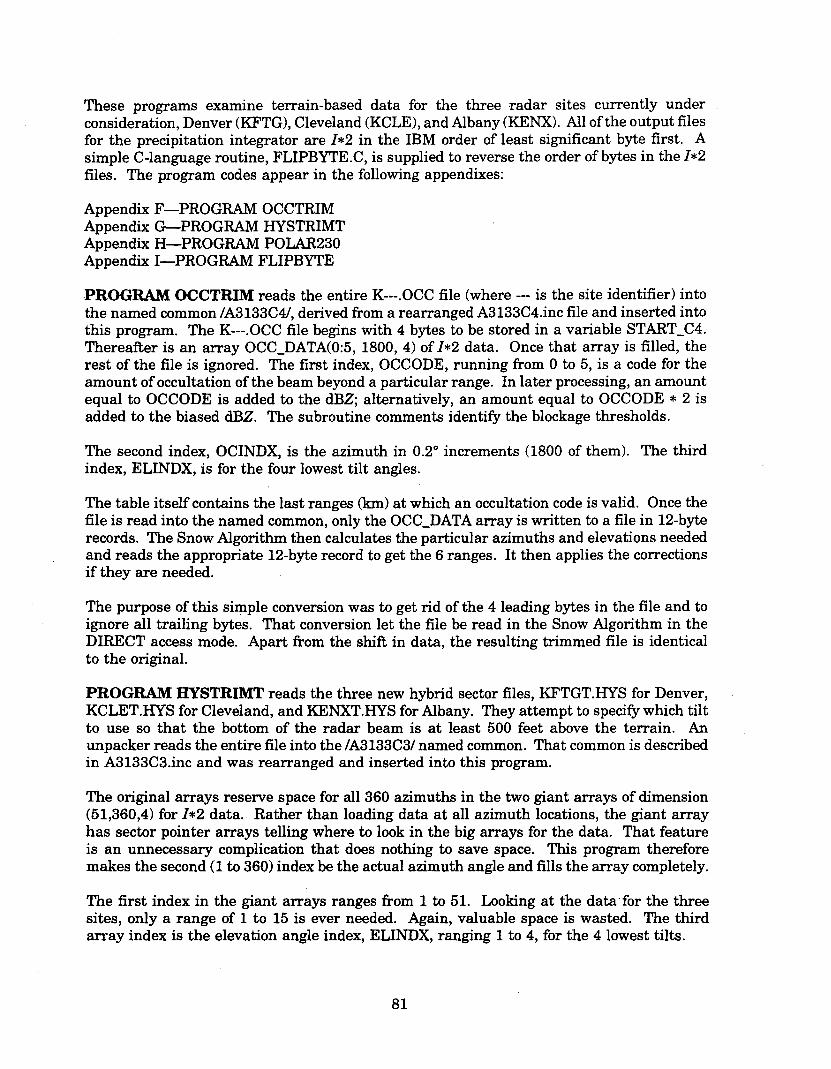
These programs examine terrain-based data for the three radar sites currently underconsideration, Denver (KFTG), Cleveland (KCLE), and Albany (KENX). All of the output filesfor the precipitation integrator are b2 in the IBM order of least significant byte first. Asimple C-Ianguage routine, FLIPBYTE.C, is supplied to reverse the order of bytes in the b2files. The program codes appear in the following appendixes:

Appendix F-PROGRAM OCCTRIMAppendix G-PROGRAM HYSTRIMTAppendix H-PROGRAM POLAR230Appendix I-PROGRAM FLIPBYTE

,PROGRAM OCCTRIM reads the entire K OCC file (where --- is the site identifier) intothe named common /A3133C4/, derived from a rearranged A3133C4.inc file and inserted intothis program. The K OCC file begins with 4 bytes to be stored in a variable START_C4.Thereafter is an array OCC_DATA(0:5, 1800, 4) of 1*2 data. Once that array is filled, therest of the file is ignored. The first index, OCCODE, running from 0 to 5, is a code for theamount of occultation of the beam beyond a particular range. In later processing, an amountequal to OCCODE is added to the dBZ; alternatively, an amount equal to OCCODE * 2 isadded to the biased dBZ. The subroutine comments identify the blockage thresholds.

The second index, OCINDX, is the azimuth in 0.20 increments (1800 of them). The thirdindex, ELINDX, is for the four lowest tilt angles.

The table itself contains the last ranges (km) at which an occultation code is valid. Once thefile is read into the named common, only the OCC_DATA array is written to a file in 12-byterecords. The Snow Algorithm then calculates the particular azimuths and elevations neededand reads the appropriate 12-byte record to get the 6 ranges. It then applies the correctionsif they are needed.

The purpose of this simple conversion was to get rid of the 4 leading bytes in the file and toignore all trailing bytes. That conversion let the file be read in the Snow Algorithm in theDIRECT access mode. Apart from the shift in data, the resulting trimmed file is identicalto the original.

PROGRAM HYSTRIMT reads the three new hybrid sector files, KFTGT.HYS for Denver,KCLET.HYS for Cleveland, and KENXT.HYS for Albany. They attempt to specify which tiltto use so that the bottom of the radar beam is at least 500 feet above the terrain. Anunpacker reads the entire file into the /A3133C3/ named common. That common is describedin A3133C3.inc and was rearranged and inserted into this program.

The original arrays reserve space for all 360 azimuths in the two giant arrays of dimension(51,360,4) for b2 data. Rather than loading data at all azimuth locations, the giant arrayhas sector pointer arrays telling where to look in the big arrays for the data. That featureis an unnecessary complication that does nothing to save space. This program thereforemakes the second (1 to 360) index be the actual azimuth angle and fills the array completely.

The first index in the giant arrays ranges from 1 to 51. Looking at the data for the threesites, only a range of 1 to 15 is ever needed. Again, valuable space is wasted. The thirdarray index is the elevation angle index, ELINDX, ranging 1 to 4, for the 4 lowest tilts.

81

The first giant array, EL_AZ_RNG(51,360,4), mostly contains pairs of ranges between whichthe reflectivities for the elevation angle indicated by ELINDX are to be used for precipitationmeasurements. When the first index = 1, the array gives the number of range pairs to followunder the rest of the first index. The largest value of EL_AZ_RNG(I,iJ) ever seen was 7,indicating that 14 range values, would be found as far as EL_AZ_RNGC15,iJ). The firstdimension was therefore shortened from 51 to 15 in the Snow Algorithm to provide a greatsavings in space.

The second giant array, XP_EL_AZ_RNG(51,360,4), had the same structure. However, theareas of tilt usage were extended from the EL_AZ_RNG array locations by 2 kIn and 2° inall directions. Therefore, the marked regions overlapped for the various tilts. The purposewas to allow the extrapolation of reflectivities from areas of no clutter to a safe distance intocluttered regions. In the May 1996 version of the snow precipitation integrator, thisextrapolation ability is ignored.

Part of this program, reflecting earlier development, wrote a file with 720-byte records thatwas more easily indexed for direct access reading. The giant arrays were reduced todimension (15,360,4). To verify that the code was working correctly, the rewritten file wasread back in and converted to an image for visualization. These parts of the program are notreally needed any more. However, the final modification is located at the end of thoseadjustments.

One can use the data in the EL_AZ_RNG array to fill 4 arrays (for each tilt) of 230 (kInrange) by 360° (degrees azimuth) with a binary indicator specifying whether to use thatparticular tilt. Every azimuth-range location will have one and only one of the four tiltsdeclared acceptable for use. The four arrays can then be condensed into a single array withvalues of 1, 2, 3, and 4 indicating the tilt (ELINDX) to use for the precipitation calculationat a particular location. The resulting array (165,600 bytes) is much easier to use than themany variables in the original /A3133C3/ named common (299,528 bytes). In this smallerversion, the named common is still in an 1*2 format, but an 1*1 format (82,800 bytes) wouldbe adequate and would save additional space. The Snow Algorithm accesses the resultingfile (HYBRDDEN.INT, HYBRDCLE.INT, or HYBRDALB.INT) as direct access. Given adesired range and azimuth, the file record number is calculated (azimuth), the record read,and the proper elevation index is read from the range-indexed array in that record.

Unfortunately, the XP_EL_AZ_RNG array cannot be written with just the tilt indices to usebecause of the overlap in areas. Adding an index for the 4 tilts would make the file 331,200bytes in the 1*1 format. That size may be suitable for direct access reading but would takeup too much space in program memory.

PROGRAM POLAR230 converts 30-arc-second digital terrain data to polar coordinates froma radar out to a range of 230 kIn. MIPS (map and image processing system) software wasused to splice and extract an array of terrain data from a set of files organized by 5° oflongitude in width. The program expects the extraction to be in multiples of whole degrees(°) in latitude and longitude. Some files are 6° oflongitude wide and others are 7° wide. Theprogram asks for top and bottom latitudes and left and right edge longitudes.

. The terrain data, in meters above mean sea level, are written to a polar coordinate array ofwidth 230 kIn and length 360° of azimuth about the specified radar site coordinates. Thearray is initialized with -999 default values.

82

On the first pass all of the latitudellongitude coordinates of the terrain, data points areconverted to the nearest radar polar coordinates by means of a great circle navigationsubroutine. The terrain elevation is then assigned to that coordinate. The process leavesgaps in the array, indicated by the -999 code.

On the second pass, all of the unused range/azimuth coordinates are converted to the nearestlatitude/longitude coordinates in 30-arc-second resolution by means of another great circlenavigation subroutine. The terrain elevation from the input file is then transferred to theradar coordinate file. All gaps are thereby filled. The file is then written to disk in 460-byteb2 records for the ranges 1 to 230 km. There are 360 records (azimuths) written. The resultis a file specifying the terrain elevation at every radar coordinate.

The program can be rewritten to use the higher resolution 3-arc-second terrain data.However, the generall-km resolution of the 30-arc-second data was considered adequate forthis test version of the software.

83

APPENDIX F

PROGRAM OCCTRIM

85

CCC

PROGRAM OCCTRIMReads Norman's occultation files *.OCC, flips bytes, stores withoutheader and trailer; get 86,400 bytes ready for direct access, *T.OCCversion of 17 April 1996, by Ed Holroyd

.

INTEGER START_C4INTEGER*2 OCC_DATA(O: 5, 1800, 4)COMMON /A3l33C4/ START_C4, OCC_DATAINTEGER*2 LINE(6)CHARACTER*l MSG,UCY,LCYCHARACTER*120CCULT1(3),OCCULT2(3)DATA OCCULT1/'KFTG.OCC ','KENX.OCCDATA OCCULT2/'KFTGT.OCC ','KENXT.OCCDATA UCY,LCY/'Y' ,'y'/OPEN(UNIT=4,FILE='PRINTER.DMP' ,STATUS='UNKNOWN')

1 WRITE(6,*)' Which site? l=Denver, 2=Albany, 3=Cleveland'READ(5,*)IDSITEOPEN(UNIT=1,FILE=OCCULT1(IDSITE),STATUS='OLD'

+,RECL=256,FORM='BINARY',IOSTAT=IOERROR)IF(IOERROR.EQ.l)WRITE(6,*)' Error opening occultation file'OPEN(UNIT=2,FILE=OCCULT2(IDSITE),STATUS='UNKNOWN'

+,RECL=12,FORM='BINARY',IOSTAT=IOERROR)IF(IOERROR.EQ.l)WRITE(6,*)' Error opening occult output file'WRITE(6,*)' Reading the array'CALL GETOCC ! to load the file into /A3133C4/: 86,404 bytesWRITE(6,*)' Writing the array'

output the arrayDO 50 K=1,4 ! tiltsDO 40 J=1,1800 ! azimuthsIF(MOD(J,100) .EQ.0)WRITE(6,*)JDO 30 I=0,5 ! occultation codes

30 LINE(I+l)=OCC_DATA(I,J,K)40 WRITE(2)LINE50 CONTINUEask for another site

WRITE(6,*)' Do you want another site?'READ(5,81)MSG

81 FORMAT (Al)IF(MSG.NE.UCY.AND.MSG.NE.LCY)GO TO 90CLOSE (1)CLOSE (2)GO TO 1 ! for a new input file selection

90 WRITE(6,*)' Normal stop'STOPEND

,, 'KCLE.OCC

,, 'KCLET.OCC

,/,/

C

C

C

CSUBROUTINE GETOCC

To unpack occultation files for NEXRAD radars and load A3133C4 arrayINTEGER*l IINBUF(256) ! input buffersINTEGER*2 INBYTE(256)

**A3133C4. inc

C** Named common definitions for the occultation data, modified for unpackingINTEGER START_C4INTEGER*2 OCC_DATA(O: 5, 1800, 4),OCCWORD(43200)EQUIVALENCE (OCC_DATA,OCCWORD)COMMON /A3133C4/ START_C4, OCC_DATA

The values in OCC_DATA are the range bins at which the occultation reachesthe indicated percentage.The first index, ranging from 0 to 6 is the occultation code:Code Occultation %

0 0-10, >60 when sample volume is part of a completely obscurredregion extending over more than 2 degrees in azimuth

11-2930-4344-5556-60

C

CCCCCCCCCC

1234

87

C 5 >60 when sample volume is part of a completely obscured regionC extending over no more than 2 degrees in azimuthC The second index is for 0.2 degree resolution data, 360 degrees * 5.C The third index is for 4 elevation levels.C convert bytes to positive integersC***************************************************************************

WRITE(6,*)' Reading occultation file'READ(l)IINBUF ! 256 bytes at a timeDO 10 I=1,256INBYTE(I)=IINBUF(I)IF(INBYTE(I) .LT.0)INBYTE(I)=INBYTE(I)+256

10 CONTINUESTART_C4=((INBYTE(1)*256+INBYTE(2))*256+INBYTE(3))*256+INBYTE(4)NWORDS=lDO 15 I=5,255,2 ! merge the bytes into 2-byte wordsOCCWORD(NWORDS)=INBYTE(I)*256+INBYTE(I+1)

15 NWORDS=NWORDS+1DO 30 J=1,336 ! read in most of the rest of the fileIF(MOD(J,30) .EQ.0)WRITE(6,*)' (336):',JREAD(l)IINBUF ! 256 bytes at a timeDO 20 I=1,256INBYTE(I)=IINBUF(I)IF(INBYTE(I) .LT.0)INBYTE(I)=INBYTE(I)+256

20 CONTINUEDO 25 I=1,255,2 ! merge the bytes into 2-byte wordsOCCWORD(NWORDS)=INBYTE(I)*256+INBYTE(I+1)

25 NWORDS=NWORDS+130 CONTINUE

READ(l)IINBUF ! 256 bytes at a time; last bufferDO 40 I=1,132 ! need only part of itINBYTE(I)=IINBUF(I)IF(INBYTE(I) .LT.0)INBYTE(I)=INBYTE(I)+256

40 CONTINUEDO 45 I=1,131,2 ! merge the bytes into 2-byte wordsOCCWORD(NWORDS)=INBYTE(I)*256+INBYTE(I+1)

45 NWORDS=NWORDS+1RETURNEND

88

APPENDIX G

PROGRAM HYSTRIMT

89

CCCCCCC

PROGRAM HYSTRIMTto trim the size of the .HYS files for three sites from 51 to 15 in oneset of dimensions. Also will fill out the EL_AZ_RNG tables to avoid theneed for a sector pointer, though that will be produced anyway. Theoutput image in AIRMAGE.DTA is for visualization. .

This version also makes an 1*2 file of 230 km x 360 degrees indicatingwhich tilt to use for hybrid sector.version of 22 April 1996, by Ed Holroyd

CHARACTER*l MSG,UCY,LCYCHARACTER*12 HYSECTRS(3),HYSTRIMS(3),HYBRDSIT'(3)DATA HYSECTRS/'KFTGT.HYS ','KENXT.HYS ','KCLET.HYS '/DATA HYSTRIMS/'KFTGTRMT.HYS', 'KENXTRMT.HYS', 'KCLETRMT.HYS'/DATA HYBRDSIT/'HYBRDDEN.INT', 'HYBRDALB.INT' ,'HYBRDCLE.INT'/DATA UCY,LCY/'Y', 'y'/OPEN(UNIT=3,FILE='ARIMAGE.DTA',STATUS='UNKNOWN' ,FORM='BINARY'

+,BLOCKSIZE=460) ! azimuth-range initial displayOPEN(UNIT=4,FILE='PRINTER.DMP',STATUS='UNKNOWN')

100 WRITE(6,*)' Which site? l=Denver, 2=Albany, 3=Cleveland'READ(5,*)IDSITEOPEN(UNIT=l,FILE=HYSTRIMS(IDSITE),STATUS='UNKNOWN' ,ACCESS='DIRECT'

+,RECL=720,FORM='UNFORMATTED',IOSTAT=IOERROR)IF(IOERROR.EQ.l)WRITE(6,*)' Error opening sector trim file'OPEN(UNIT=2,FILE=HYSECTRS(IDSITE),STATUS='OLD' ,ACCESS='DIRECT'

+,RECL=256,FORM='UNFORMATTED',IOSTAT=IOERROR)IF(IOERROR.EQ.l)WRITE(6,*)' Error opening sector file'OPEN(UNIT=7,FILE=HYBRDSIT(IDSITE),STATUS='UNKNOWN' ,FORM='BINARY'

+,BLOCKSIZE=460) ! hybrid sectors in polar coordinatesCALL GETHYS ! to load the file into /A3133C3/: 299,524 bytesCALL PUTHYS ! to write the trimmed fileCALL GETHYS2 ! to read back trimmed fileWRITE(6,*)' Do you want another file?'READ(5,81)MSG

81 FORMAT (Al)IF(MSG.NE.UCY.AND.MSG.NE.LCY)GO TO 90GO TO 100 ! for a new input file selection

90 WRITE(6,*)' Normal stop'STOPE~

CSUBROUTINE GETHYS

To unpack occultation files for NEXRAD radars and load A3133C3 arrayINTEGER*l IINBUF(256) ! input buffersINTEGER*2 INBYTE(256)

**A3133C3.incC** Named common for the elevation, range, and azimuth sector adaptationC** tables

.

INTEGER START_C3,AZBOUNDS(360),SECTOR_PNTR(360)INTEGER*2 EL_AZ_RNG(51,360,4),ELWORD(73440)INTEGER XP_AZBOUNDS(360),XP_SECTOR_PNTR(360)INTEGER*2 XP_EL_AZ_RNG(51,360,4),XPWORD(73440) .

EQUIVALENCE(EL_AZ_RNG,ELWORD), (XP_EL_AZ_RNG,XPWORD)COMMON /A3133C3/ START_C3, AZBOUNDS, SECTOR_PNTR, EL_AZ_RNG,

$ XP_AZBOUNDS, XP_SECTOR_PNTR, XP_EL_AZ_RNGC convert bytes to positive integersC***************************************************************************

WRITE(6,*)' Reading .HYS file into /A3133C3/'READ(2)IINBUF ! 256 bytes at a timeDO 10 1=1,256INBYTE(I)=IINBUF(I)IF(INBYTE(I) .LT. 0)INBYTE(I) =INBYTE(I) +256

10 CONTINUESTART_C3=((INBYTE(1)*256+INBYTE(2))*256+INBYTE(3))*256+INBYTE(4)NWORDS=l

.

WRITE(6,*)' Loading AZBOUNDS'DO 12 1=5,253,4 ! merge the bytes into first 63 4-byte words

C

91

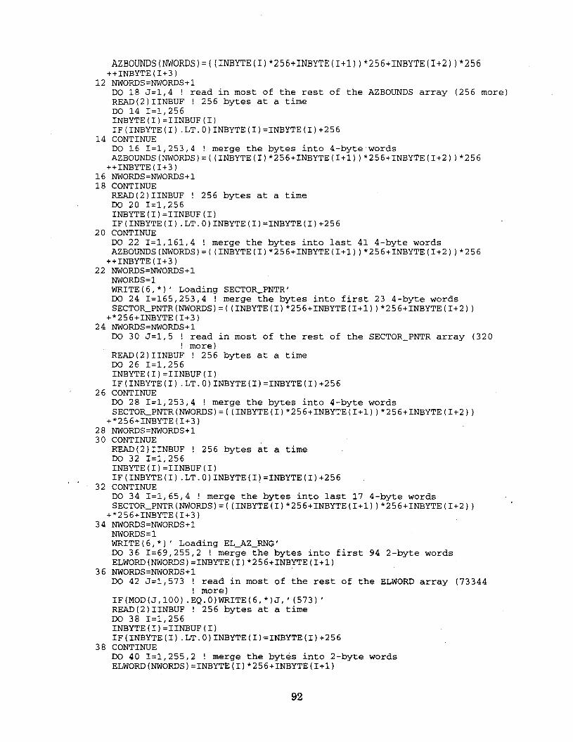
AZBOUNDS(NWORDS)=((1NBYTE(1)*256+1NBYTE(1+1))*256+1NBYTE(1+2))*256++INBYTE(I+3)

12 NWORDS=NWORDS+1DO 18 J=1,4 ! read in most of the rest of the AZBOUNDS array (256 more)READ(2)IINBUF ! 256 bytes at a timeDO 14 1=1,256INBYTE(I)=IINBUF(I)IF(INBYTE(I) .LT.0)INBYTE(I)=INBYTE(I)+256

14 CONTINUEDO 16 1=1,253,4 ! merge the bytes into 4-byte'wordsAZBOUNDS(NWORDS)=((INBYTE(I)*256+INBYTE(I+1))*256+INBYTE(1+2))*256++INBYTE(I+3)

16 NWORDS=NWORDS+118 CONTINUE

READ(2)IINBUF ! 256 bytes at a timeDO 20 1=1,256INBYTE(I) =IINBUF (I)IF(INBYTE(I) .LT.0)INBYTE(I)=INBYTE(I)+256

20 CONTINUEDO 22 1=1,161,4 ! merge the bytes into last 41 4-byte wordsAZBOUNDS(NWORDS)=((INBYTE(I)*256+INBYTE(I+1))*256+INBYTE(1+2) )*256

++INBYTE(I+3)22 NWORDS=NWORDS+1

NWORDS=lWRITE(6,*)' Loading SECTOR_PNTR'DO 24 1=165,253,4 ! merge the bytes into first 23 4-byte wordsSECTOR_PNTR(NWORDS)=((INBYTE(I)*256+INBYTE(I+1))*256+INBYTE(I+2))

+*256+INBYTE(I+3)24 NWORDS=NWORDS+1

DO 30 J=l,5 ! read in most of the rest of the SECTOR_PNTR array (320! more)

READ(2)IINBUF ! 256 bytes at a timeDO 26 1=1,256INBYTE(I)=IINBUF(I)IF(INBYTE(I) .LT.O) INBYTE(I) =INBYTE(I) +256

26 CONTINUEDO 28 1=1,253,4 ! merge the bytes into 4-byte wordsSECTOR_PNTR(NWORDS)=((INBYTE(I)*256+INBYTE(I+1))*256+INBYTE(I+2))

+*256+INBYTE(I+3)28 NWORDS=NWORDS+130 CONTINUE

READ(2)IINBUF ! 256 bytes at a timeDO 32 1=1,256INBYTE(I)=IINBUF(I)IF(INBYTE(I) .LT.0)INBYTE(I)=INBYTE(I)+256

32 CONTINUE '

DO 34 1=1,65,4 ! merge the bytes into last 17 4-byte wordsSECTOR_PNTR(NWORDS)=((INBYTE(I)*256+INBYTE(I+1))*256+INBYTE(I+2))

+*256+INBYTE(I+3)34 NWORDS=NWORDS+1

NWORDS=lWRITE(6,*)' Loading EL_AZ_RNG'DO 36 1=69,255,2 ! merge the bytes into first 94 2-byte wordsELWORD(NWORDS)=INBYTE(I)*256+INBYTE(I+1)

36 NWORDS=NWORDS+ 1DO 42 J=l,573 ! read in most of the rest of the ELWORD array (73344

! more)IF(MOD(J,100) .EQ.0)WRITE(6,*)J,' (573)'READ(2)IINBUF ! 256 bytes at a timeDO 38 1=1,256INBYTE(I)=IINBUF(I)IF(INBYTE(I) .LT.0)INBYTE(I)=INBYTE(I)+256

38 CONTINUEDO 40 1=1,255,2 ! merge the bytes into 2-byte wordsELWORD(NWORDS)=INBYTE(I)*256+INBYTE(I+1)

92

40 NWORDS=NWORDS+142 CONTINUE

READ(2)IINBUF ! 256 bytes at a timeDO 44 I=1,256INBYTE(I) =IINBUF (I)IF(INBYTE(I) .LT.0)INBYTE(I)=INBYTE(I)+256

44 CONTINUEDO 46 I=1,3,2 ! merge the bytes into last 2 2-byte wordsELWORD(NWORDS)=INBYTE(I)*256+INBYTE(I+1)

46 NWORDS=NWORDS+1NWORDS=lWRITE(6,*)' Loading XP_AZBOUNDS'DO 48 I=5,253,4 ! merge the bytes into first 63 4-byte wordsXP_AZBOUNDS(NWORDS)=((INBYTE(I)*256+INBYTE(I+1))*256+INBYTE(I+2))

+*256+INBYTE(I+3)48 NWORDS=NWORDS+1

DO 54 J=1,4 ! read in most of the rest of the XP_AZBOUNDS array (256! more)

READ(2)IINBUF ! 256 bytes at a timeDO 50 I=1,256INBYTE(I)=IINBUF(I)IF(INBYTE(I) .LT.0)INBYTE(I)=INBYTE(I)+256

50 CONTINUEDO 52 I=l,253,4 ! merge the bytes into 4-byte wordsXP_AZBOUNDS(NWORDS)=((INBYTE(I)*256+INBYTE(I+1))*256+INBYTE(I+2))

+*256+INBYTE(I+3)52 NWORDS=NWORDS+154 CONTINUE

READ(2)IINBUF ! 256 bytes at a timeDO 56 I=l,256INBYTE(I)=IINBUF(I)IF(INBYTE(I) .LT.0)INBYTE(I)=INBYTE(I)+256

56 CONTINUEDO 58 I=l,161,4 ! merge the bytes into last 41 4-byte wordsXP_AZBOUNDS(NWORDS)=((INBYTE(I)*256+INBYTE(I+1))*256+INBYTE(I+2))

+*256+INBYTE(I+3)58 NWORDS=NWORDS+1

NWORDS=lWRITE(6,*)' Loading XP_SECTOR_PNTR'DO 60 I=165,253,4 ! merge the bytes into first 23 4-byte wordsXP_SECTOR_PNTR(NWORDS)=((INBYTE(I)*256+INBYTE(I+1))*256

++INBYTE(I+2))*256+INBYTE(I+3)60 NWORDS=NWORDS+1

DO 66 J=l,5 ! read in most of the rest of the XP_SECTOR_PNTR array (320! more)

READ(2)IINBUF ! 256 bytes at a timeDO 62 I=l, 256INBYTE(I)=IINBUF(I)IF(INBYTE(I) .LT. 0)INBYTE(I)=INBYTE(I) +256

62 CONTINUEDO 64 I=l,253,4 ! merge the bytes into 4-byte wordsXP_SECTOR_PNTR(NWORDS)=((INBYTE(I)*256+INBYTE(I+1))*256

++INBYTE(I+2))*256+INBYTE(I+3)64 NWORDS=NWORDS+166 CONTINUE

READ(2)IINBUF ! 256 bytes at a timeDO 68 I=l,256INBYTE(I)=IINBUF(I)IF (INBYTE (I) .LT.0)INBYTE(I)=INBYTE(I)+256

68 CONTINUEDO 70 I=l,65,4 ! merge the bytes into last 17 4-byte wordsXP_SECTOR_PNTR(NWORDS)=((INBYTE(I)*256+INBYTE(I+1))*256

++INBYTE(I+2))*256+INBYTE(I+3)70 NWORDS=NWORDS+l

NWORDS=l

93

WRITE(6,*)' Loading XP_EL_AZ_RNG'DO 72 I=69,255,2 ! merge the bytes into first 94 2-byte wordsXPWORD(NWORDS)=INBYTE(I)*256+INBYTE(I+l)

72 NWORDS=NWORDS+lDO 78 J=1,573 ! read in most of the rest of the ELWORD array (73344

! more)IF,(MOD(J,lOO) .EQ.0)WRITE(6,*)J,' (573)'READ(2)IINBUF ! 256 bytes at a timeDO 74 I=1,256INBYTE(I)=IINBUF(I)IF(INBYTE(I) .LT.0)INBYTE(I)=INBYTE(I)+256

74 CONTINUEDO 76 I=1,255,2 ! merge the bytes into 2-byte wordsXPWORD(NWORDS)=INBYTE(I)*256+INBYTE(I+l)

76 NWORDS=NWORDS+l78 CONTINUE

READ(2)IINBUF ! 256 bytes at a timeDO 80 I=1,256INBYTE(I)=IINBUF(I)IF(INBYTE(I) .LT.0)INBYTE(I)=INBYTE(I)+256

80 CONTINUEDO 82 I=1,3,2 ! merge the bytes into last 2 2-byte wordsXPWORD(NWORDS)=INBYTE(I)*256+INBYTE(I+l)

82 NWORDS=NWORDS+lRETURNEND

C

CSUBROUTINE PUTHYS

writes a truncated version of /A3133C3/ to disk using 720 byte I*2 recordsINTEGER*2 OUTWORD(360),STA(2),AZB(720),SEC(720),XPA(720),XPS(720)EQUIVALENCE (START_C3,STA), (AZBOUNDS,AZB), (SECTOR_PNTR,SEC)

+, (XP_AZBOUNDS,XPA), (XP_SECTOR_PNTR,XPS)**A3133C3. incC** Named common for the elevation, range, and azimuth sector adaptationC** tables

INTEGER START_C3,AZBOUNDS(360),SECTOR_PNTR(360)INTEGER*2 EL_AZ_RNG(51,360,4)INTEGER XP_AZBOUNDS (360)" XP_SECTOR_PNTR (360 )

INTEGER*2 XP_EL_AZ_RNG(51,360,4)COMMON /A3133C3/ START_C3, AZBOUNDS, SECTOR_PNTR, EL_AZ_RNG,

$ XP_AZBOUNDS, XP_SECTOR_PNTR, XP_EL_AZ_RNGC************************************************************************

OUTWORD(l)=STA(l)OUTWORD(2)=STA(2)DO 1 J=3,360

1 OUTWORD(J)=O ! blank filIon first record toWRITE(l,REC=l)OUTWORD ! all 720 bytesDO 10 J=1,360

10 OUTWORD(J)=AZB(J)WRITE (1,REC=2)OUTWORDDO 12 J=1,360

12 OUTWORD(J)=AZB(J+360)WRITE (1,REC=3)OUTWORDDO 14 J=1,360

14 OUTWORD(J)=SEC(J)WRITE(1,REC=4)OUTWORDDO 16 J=1,360

16 OUTWORD(J)=SEC(J+360)WRITE(1,REC=5)OUTWORDNREC=6DO 30 K=1,4DO 30 I=1,15 ! not the 51 availableDO 20 J=1,360JJ=SECTOR_PNTR(J) ! to eliminate the need for this array

20 OUTWORD(J)=EL_AZ_RNG(I,JJ,K) ! fill out the 360 dimension

94

WRITE (1,REC=NREC) OUTWORD30 NREC=NREC+l

DO 40 J=1,36040 OUTWORD(J)=XPA(J)

WRITE (l,REC=NREC) OUTWORDNREC =NREC + 1

DO 42 J=1,36042 OUTWORD(J)=XPA(J+360)

WRITE (1,REC=NREC)OUTWORDNREC =NREC + 1

DO 44 J=1,36044 OUTWORD(J)=XPS(J)

WRITE (1,REC=NREC) OUTWORDNREC=NREC+lDO 46 J=1,360

46 OUTWORD(J)=XPS(J+360)WRITE (1,REC=NREC)OUTWORDNREC=NREC+lDO 60 K=1,4DO 60 I=1,15 ! not the 51 availableDO 50 J=1,360JJ=XP_SECTOR_PNTR(J) ! to eliminate the need for this array

50 OUTWORD(J)=XP_EL_AZ_RNG(I,JJ,K) ! fill out the 360 dimensionWRITE (1,REC=NREC) OUTWORD

60 NREC=NREC+lRETURNEND

C

CC

SUBROUTINE GETHYS2 .

To unpack trimmed hybrid sector files for NEXRAD radars and load /A3133C3/from disk using 720 byte I*2 records

INTEGER*2 INWORD(360),STA(2),AZB(720),SEC(720),XPA(720),XPS(720)+, LINE (230)

EQUIVALENCE (START_C3,STA), (AZBOUNDS,AZB), (SECTOR_PNTR,SEC)+, (XP_AZBOUNDS,XPA), (XP_SECTOR_PNTR,XPS)

**A3133C3.inc

C** Named common for the elevation, range, and azimuth sector adaptationC** tables

INTEGER START_C3,AZBOUNDS(360),SECTOR_PNTR(360)INTEGER*2 EL_AZ_RNG(51,360,4) ! 51 changes to 15 in other programINTEGER XP_AZBOUNDS(360),XP_SECTOR_PNTR(360)INTEGER*2 XP_EL_AZ_RNG(51,360,4) ! 51 changes to 15 in other programCOMMON /A3133C3/ START_C3, AZBOUNDS, SECTOR_PNTR, EL_AZ_RNG,

$ XP_AZBOUNDS, XP_SECTOR_PNTR, XP_EL_AZ_RNGC************************************************************************

WRITE(6,*)' Reading back hybrid sector file'READ(l,REC=l)INWORD ! all 720 bytesSTA(l)=INWORD(l)STA(2)=INWORD(2)READ(1,REC=2)1NWORDDO 10 J=1,360

10 AZB(J)=INWORD(J)READ(1,REC=3)INWORDDO 12 J=1,360

12 AZB(J+360)=INWORD(J)READ(1,REC=4)INWORDDO 14 J=1,360

14 SEC(J)=1NWORD(J)READ(1,REC=5)1NWORDDO 16 J=1,360

16 SEC(J+360)=1NWORD(J)'NREC=6DO 30 K=1,4DO 30 1=1,15 ! not the 51 originally in the named commonREAD(l,REC=NREC)INWORD

95

C

DO 20 J=l,36020 EL_AZ_RNG(I,J,K)=INWORD(J)30 NREC=NREC+1

READ(l,REC=NREC)INWORDDO 40 J=l,360

40 XPA(J)=INWORD(J)NREC=NREC+1READ(l,REC=NREC)INWORDDO 42 J=l,360

42 XPA(J+360)=INWORD(J)NREC =NREC + 1

READ(l,REC=NREC)INWORDDO 44 J=l,360

44 XPS(J)=INWORD(J)NREC=NREC+1READ(l,REC=NREC)INWORDDO 46 J=l,360

46 XPS(J+360)=INWORD(J)NREC =NREC + 1

DO 60 K=1,4DO 60 I=l,15 ! not the 51READ(l,REC=NREC)INWORDDO 50 J=l,360

50 XP_EL_AZ_RNG(I,J,K)=INWORD(J)60 NREC=NREC+1Write an image file showing the large arrays for hybrid sectors

DO 70 K=l,4DO 70 J=l,360DO 61 I=l,230

61 LINE(I)=l ! clean the output lineN=EL_AZ_RNG(l,J,K) ! count of range pairs to followIP=lDO 64 NP=l,N ! pairs loopIP=IP+1IBEG=EL_AZ_RNG(IP,J,K) ! beginning rangeIP=IP+1IEND=EL_AZ_RNG(IP,J,K) ! ending rangeDO 62 I=IBEG,IEND ! fill loop

62 LINE(I)=K+1 ! load with the elevation index + 164 CONTINUE! pairs loop70 WRITE(3)LINE ! image outputWrite a hybrid sector file in polar coordinates

DO 80 J=l,360 ! azimuth loopDO 71 1=1,230

71 LINE(I)=O l clean the output line; all zeros should be replacedDO 76 K=1,4 ! tilts loopN=EL_AZ_RNG(l,J,K) ! count of range pairs to followIP=lDO 74 NP=l,N ! pairs loopIP=IP+1IBEG=EL_AZ_RNG(IP,J,K) ! beginning rangeIP=IP+1IEND=EL_AZ_RNG(IP,J,K) l ending rangeDO 72 I=IBEG,IEND ! fill loopIF(LINE(I) .EQ.O)LINE(I)=K l update with the elevation index

72 CONTINUE! fill loop74 CONTINUE l pairs loop76 CONTINUE! tilts loop80 WRITE(7)LINE l hybrid sector output, end of azimuth loopWrite an image file showing the large arrays for expanded sectors

DO 90 K=l,4DO 90 J=l,360DO 81 1=1,230

81 LINE(I)=l ! clean the output lineN=XP_EL_AZ_RNG(l,J,K) ! count of range pairs to follow

C

C

96

IP=lDO 84 NP=l,N ! pairs loopIP=IP+lIBEG=XP_EL_AZ_RNG(IP,J,K) ! beginning rangeIP=IP+lIEND=XP_EL_AZ_RNG(IP,J,K) ! ending rangeDO 82 I=IBEG,IEND ! fill loop

82 LINE(I)=K+l ! load with the elevation index84 CONTINUE! pairs loop90 WRITE(3)LINE ! image output

RETURNEND

97

98

APPENDIX H

PROGRAM POLAR230

99

CC

PROGRAM POLAR230Converts 30 arc-see DEM elevations to polar coordinates from a radar.Version of 8 April 1996 by Ed Holroyd

COMMON /LATLON/ ALAT,ALON,AD,R,RLAT,RLONDOUBLE PRECISION ALAT,ALON,AD,R,RLAT,RLONINTEGER*2 INBUF6(721) ,INBUF7(841) ! for arrays 6 and 7 degrees wideEQUIVALENCE (INBUF6,INBUF7)INTEGER*2 LAND(360,230),OUTBUF(230)CHARACTER*30 INFILECHARACTER*l MSG,UCY,LCYDATA UCY,LCY/'Y', 'y'/DECD(ND,NM,SEC)=FLOAT(ND)+FLOAT(NM)/60.+SEC/3600.OPEN(UNIT=2,FILE='POLARDEM.DMP' ,STATUS='UNKNOWN' ,FORM='BINARY'+, BLOCKSIZE=460) ! I*2 elevations, meters, to 230 kmOPEN(UNIT=4,FILE='PRINTER.DMP' ,STATUS='UNKNOWN')WRITE(6,*)' Type input DEM data file name'READ(5,1)INFILE

1 FORMAT (A30)WRITE(6,*)' Type N latitude of top of array (whole degrees)'READ(5,*)LATTWRITE(6,*)' Type N latitude of bottom of array'READ(5,*)LATBWRITE(6,*)' Type W longitude of left of array (whole degrees)'READ(5,*)LONLWRITE(6,*)' Type W longitude of right of array'READ(5,*)LONRLATN=(LATT-LATB)*120+1 ! number of lines in arrayLONN=(LONL-LONR)*120+1 ! number of columns in arrayWRITE(4,*)' LATN,LONN=' ,LATN,LONNWRITE(6,*)' LATN,LONN=' ,LATN,LONNNBYTES=LONN*2 ! for I*2 elevation data, metersOPEN(UNIT=l,FILE=INFILE,STATUS='OLD',MODE='READ' ,FORM='BINARY'

+,ACCESS='DIRECT' ,RECL=NBYTES,BLOCKSIZE=NBYTES)DO 2 I=1,360 ! degreesDO 2 J=1,230 ! km

2 LAND(I,J)=-999 ! initialization to nearly 1 km below sea levelWRITE(6,*)' Type radar N latitude, dd,mm,ss.'READ(5,*)LATD,LATM,SLATRLAT=DECD(LATD, LATM, SLAT)WRITE(6,*)' Type radar W longitude, ddd,mm,ss.'READ(5,*)LOND,LONM,SLONRLON=DECD(LOND, LONM, SLON)

5 LINES=OBegin sequential reading through entire file

10 IF(LONN.EQ.721)READ(1,ERR=90)INBUF6IF(LONN.EQ.841)READ(1,ERR=90)INBUF7LINES=LINES+1ALAT=FLOAT(LATT)-FLOAT(LINES-1)/120.

. IF (MOD (LINES, 12) .EQ.1)WRITE(6,*)' Latitude now' ,ALATDO 20 K=l,LONN ! scan along all longitudes, eastwardALON=FLOAT(LONL)-FLOAT(K-1)/120.CALL GTCIRC ! get R, AD radar coordinates for that locationI=IDNINT(AD) ! rounded azimuth, degreesJ=IDNINT(R) ! rounded range, kmIF(I.LT.1.0R.I.GT.360)I=360IF(J.LT.1)J=1IF(J.GT.230)GO TO 20 ! too far out, skip it

nearest neighbor assignment of elevations:IF(LONN.EQ.721)LAND(I,J)=INBUF6(K)IF(LONN.EQ.841)LAND(I,J) =INBUF7 (K)

20 CONTINUE! eastward scanIF(LINES.LT.LATN)GOTO 10 ! for another line of data

search for data voidsDO 30 J=1,230R=J ! km

CC

C

C

C

101

N=ODO 25 1=1,360AD=I ! degreesIF(LAND(I,J) .EQ.-999.)THEN ! calculate nearest DEM pixel location

CALL LALONG ! for latitude ALAT, longitude ALON of that range binL=(FLOAT(LATT)-ALAT)*120.+1.5 ! rounded line numberIF(LONN.EQ.721)READ(1,REC=L,ERR=90)INBUF6IF(LONN.EQ. 841)READ(1,REC=L,ERR=90) INBUF7K=(FLOAT(LONL)-ALON)*120.+1.5 ! rounded column numberLAND(I,J)=INBUF6(K) ! nearest neighbor assignmentN=N+1

ENDIF25 CONTINUE

IF(N.GT.O)THENWRITE(4,*)' Voids filled at range' ,J,NWRITE(6,*)' Voids filled at range' ,J,N

ENDIF30 CONTINUE

DO 80 1=1,360DO 70 J=1,230

70 OUTBUF(J)=LAND(I,J)WRITE (2)OUTBUFIF(MOD(I,10) .EQ.0)WRITE(6,*)' Output, azimuth=' ,I

80 CONTINUE90 WRITE(6,*)' normal stop'

STOPEND

C

CCC

SUBROUTINE GTCIRC .

Converts latitude, longitude (fractional degrees) of ALAT, ALON intorange and azimuth from origin at RLAT, RLON (also fractional degrees).Range R will be in km, azimuth AD in degrees.

COMMON /LATLON/ ALAT,ALON,AD,R,RLAT,RLONDOUBLE PRECISION ALAT,ALON,AD,R,RLAT,RLONDOUBLE PRECISION OLAT,OLON,DLAT,DLON,DR,SCS,SC,X,DA,PR,C,SDATA PR/.017453293D+00/

COLAT=PR*RLATOLON=PR*RLON .

DLAT=PR*ALATDLON=PR*ALONC=DSIN(OLAT) *DSIN(DLAT) +DCOS (OLAT) *DCOS(DLAT)*DCOS(DLON-OL ON)IF (C .GT.1. )C=1.

IF(C.LT.-1.)C=-1.DR=DACOS(C)SCS=DSIN(DLAT)-C*DSIN(OLAT)SC=DSIN(DR)*DCOS(OLAT)IF(SC.EQ.O.)GO TO 10X=SCS/SCIF(X.GT.1. )X=1.IF(X.LT.-1.)X=-1.A=DACOS(X)R=DR*6377.59D+00 ! or whatever earth radius (km) you want to use.IF (DLON.GT.OLON)A=-AAD=A/PRIF(AD.LT.0.)AD=AD+360.RETURN

10 A=O.AD=O.RETURN

C

CCC

ENTRY LALONGConverts azimuth AD (degrees) and range R (km) from origin RLAT, RLON(fractional degrees) into destination latitude ALAT and longitude ALON(fractional degrees).

102

OLAT=PR*RLATOLON=PR*RLONDR=R/6377.S9D+OO ! from earth radius in kmIF(AD.LT.O.)AD=AD+360.A=AD*PRDA=AIFLG=OIF(AD.LE.180)IFLG=1S=DCOS(DA) *DSIN(DR) *DCOS(OLAT) +DCOS (DR) *DSIN(OLAT)IF (S. GT .1. )S=l.IF(S.LT.-1.)S=-1.DLAT=DASIN(S)C=(DCOS(DR)-DSIN(OLAT)*DSIN(DLAT))/(DCOS(OLAT)*DCOS(DLAT))IF(C.GT.l. )C=l.IF(C.LT.-1.)C=-1.DLON=DACOS(C)IF(IFLG.EQ.1)DLON=-DLONALON=(OLON+DLON)/PRALAT=DLAT/PRRETURNEND

103

APPENDIX I

PROGRAM FLIPBYTE

105

#include <stdio.h> /*input-output*//* FLIPBYTE.C a program to interchange 1*2 bytes */

/* DEFINE GLOBAL VARIABLES */char inbyte[16384], outbyte[16384],int count=O, i=O;long m=O, n=O, count1=O, count2=O;FILE *fp1, *fp2;

infile[32], outfile[32];

main ( )

{questions(); /* OPENING DIALOGUE */while((count = fread(inbyte,1,16384,fp1)) != O){

i=O;while (i<count){

outbyte[i+1]=inbyte[i];outbyte[i]=inbyte[i+1];n += 1;count2 += 1;if(n == m){

printf ("byte pairs flipped: %ld\r",count2) ;n=O;}

i+=2;} /* END OF WHILE FLIP LOOP */

count1 = fwrite(outbyte,1,count,fp2)/2;} /* END OF WHILE READ LOOP */

printf("Final byte pairs flipped: %ld\n",count2);} /* END OF PROGRAM */

questions ( )

{

printf ("Type input file name: ");scanf("%s",infile) ;fp1=fopen(infile, "rb");if (fp1 == NULL) {

printf("Couldn't open %s\n",infile);exi t (1) ;

}

printf("Type output file name: ");scanf("%s",outfile);fp2=fopen(outfile, "wb");if (fp2 == NULL) {

printf ("Couldn' t open %s \n" ,outfile) ;exi t (2) ;

}printf("How many bytes for message frequency: ");scanf (

"%id" ,&m) ;}

/* FUNCTION FOR OPENING DIALOGUE */

107

APPENDIX J

Comparison Between OSF and Reclamation Routines

109

Changes in PPS and VAD routines that appear in the Snow Algorithm (May 1996 version).

A3133D_INIT_ADAPT

Removed (ADPT_PARAMS) from passed parameters. Replaced all (CONSTANT) pointersand used adaptable parameters list from a file with a direct definition (not read in) insteadof using =ADPT_PARAMS(pointer). Removed the include lines that obtained those constantpointers. Rearranged A3133CA.inc and inserted it. Removed the REAL ADPT_PARAMS andDATA lines. Removed all UPDATE_TABLE lines. Removed excessive comments and debugstatements.

These parameters have been changed from those in the file:ZR_MLT_COEFF =399. (for equation (5))

=318. (for Cleveland, Ohio, equation (8))=155. (for Denver, CO, equation (9))

ZR_PWR_COEF =2.21 (for equation (5))=1.5 (for Cleveland, Ohio, equation (7))=1.6 (for Denver, CO, equation (8))

MINTHRFL=-10.MIN_DBZ_AR- WGTD=-10.MIN_DBZ=-10.

NOTE: The original PPS version of A3133D is acceptable when the program is rewritten byOSF. The five variables are more properly changed in the file for the adaptable parametersaccording to OSF style and specifications. .

A3133F _FILL_PRECIP _TABLE

Removed debug statements and excessive comment lines. Rearranged A3133CA.inc andinserted it. Replaced all (CONSTANT) values with their numbers and eliminated the relatedinclude statements. Retained only the REAL MIN_DBZ, MAJCDBZ line of the typedeclarations and distributed the parameter values where needed.

IMPORTANT CHANGE: Changed from 10ths of mmlh to 100ths of mmlh for betterresolution. See line 200 RATE_TABLE(I)= Also changed MIN_NONZERO_RATE to.005 mmlh for snow.

A317G2- VAD_PROC

None of the include files is needed. The /A317VAI and /A317VD/ common blocks are notreferenced. The debug statements and excessive comments have been removed. The REALand INTEGER declarations are removed. Most of the PARAMETER definitions aredistributed if needed.

Added the /STORE/, /TESTS/, and /WINDV/ named commons.

111

Substituted everywhere (old version --> new version):. FIT_TESTS --> NFIT (arbitrarily defined as 3 elsewhere). CELV --> K (index equal to kft level). NPT --> NK (point count). HWD --> DK (horizontal wind direction). SHW --> SK (horizontal wind speed). RMS --> RMSK (r.m.s.). 7 --> 17 (DO loop index). MINPTS --> 15 (arbitrary 15-point requirement)

. Added DO 40 K=I,15 ! kft to cycle through first 15 kft levels above sea level.

. Removed from all called subroutine parameters: NAZIMS, NRADIALS, MISSING, AZM,VE and added K.

. In IF(CF3.NE.0 ) changed AND to OR. Then changed HWD(CELV) to DKR in fourstatements except the last: HWD(CELV)=HWD(CELV)IDTR --> DK(K)=DKRlDTR.

. Removed references to WMODE, HT_SEA, and PFV.

. Removed ICOS(ELV_RAD) because the speeds were already adjusted to horizontal insubroutine GETPROF.

. Added SK(K)=-99. to indicate bad or missing wind speeds.

. Removed call to A317L2.

A317H2- VAD_LSF

Removed NAZIMS, NRADIALS, MISSING, AZM, VE from call parameters and added K.Removed debug statements and excessive comments. Retained only DNPT and TWO_N asINTEGER. Removed REAL statements. Added ISTOREI named common. Removed DTReverywhere by using trig functions in degrees (°):. SIN --> SIND (sine in degrees [°]). COS --> COSD (cosine in degrees [°]). AZM_RAD --> A (azimuth). VE(I) --> FLOAT(IV(K,J,I)/lO. ! 110. to get back to m S.l (wind speed)

. Added CFl=CF2=CF3=-9999. for missing values and removed the many =MISSING lines.later.

. Added loop DO 12 J=I,360 ! azimuths to cycle through all azimuths.

. Moved SIN_AZ=SIND(A) and COS_AZ=COSD(A) forward and addedSIN_2AZ=SIND(2.*A) and COS_2AZ=COSD(2.*A) for substitution later.

. Added ILIM lines to work through all data entries.

. Changed DO 10 I=I,NRADIALS to I,ILIM.. Changed IF(VE(I).GT.MISSING)THEN structure to IF(IV(K,J,I).EQ.-9999)GO TO 10.

The important complex calculations are not changed at all.

A317I2- VAD_RMS

Removed NAZIMS, NRADIALS, MISSING, AZM, VE from call parameters and added K.Removed debug statements and excessive comments. Removed all DTR lines. Removed alltype declarations except INTEGER DNPT. Added ISTOREI named common.

112

. Added loop DO 12 J=1,360 ! azimuths to cycle through all azimuths.

. Added A=FLOAT(J)-.5 as a substitute for AZM(I).

. Added ILIM lines to work through all data entries.

. Changed DO 10 I=l,NRADIALS to 1,ILIM.

. Changed VE(I) to IV(K,J,I) and MISSING to -9999. Defined VE=FLOAT(IV(K,J,I»/10.to convert speed to m S-l.

. Changed COS to COSD for angles in degrees (°).

A317J2_FIT_TEST

Removed NAZIMS, NRADIALS, MISSING, AZM, VE from call parameters and added K.Removed debug statements and excessive comments. Removed all DTR lines. Removed alltype declarations. Added /STORE/ named common.

. Added loop DO 12 J=1,360 ! azimuths to cycle through all azimuths.

. Added A=FLOAT(J)-.5 as a substitute for AZM(I).

. Added ILIM lines to work through all data entries.

. Changed DO 10 I=l,NRADIALS to 1,ILIM.

. Changed VE(I) to IV(K,J,I) and MISSING to -9999. Defined VE=FLOAT(IV(K,J,I)/10.to convert speed to m S-land substitute for VE(I).

. Changed COS to COSD for angles in degrees (°).

. Shortened some IF statements.

A317K2_SYM_CHK

Removed debug and excessive comments. Removed type declarations except for LOGICALSYM.

113

-APPENDIX K

PROGRAM RDNX.C

115

RDNX" C

/* open and read NEXRAD file as unformated reads function on a DOS PC. If it isfound that C2432 starts the 24 characters .Please open NEXRAD file., then whatfollows up to a null byte is taken to be the name of a file to open and readboth the first 24 bytes starting -ARCHIVE2.. into C24, and the first whatever it

is of expected standard radial size 2432 bytes into C2432. Other calls to herewill continue from where last left off and read in the next 2432 bytes (or ofwhatever specified size *2 +8*2) into C2432. ./linclude<stdio. h>

I"standard I/O functions etc. ../

linc!ude<ctype. h> /*standard character & string processing routines

*I

struct comCBUF{ uns~gned char C24[24]; unsigned char C2432f2432];) ;

extern struct comCBUF cbuf ;

/* for COMMON ICBUFI C24, C2432 *1void rdnexrad ( Hsg )

int *Ms9; 1* set=

bytes read in, or -1 if read error */{static FILE *pIn; 1* prt to input file to read *1int I,J,L=O,H, 1* for various indices etc. */

IFEOF=O; 1* to remember if EoF hit*

Istatic int IsOpnd=O; 1* to remember if file has been opened *1static char PlzOpn(]={ -Please open NEXRAD file -),

ARCHIVE2 I J=

( . ARCHIVE2 . );

for (1=0; 1<24; 1++) if (PlzOpn[I]!=cbuf_.C2432[I]) goto NxtRec;1* caller has indicated a new file is to be opened so first close old (if any)

*I

if (lsOpnd) fclose(pln);if «pIn=fopen(cbuf_.C2432+24,-r-»==NULL) 1* if bad named file to read *1(

printf(-unable to open 's\n-, cbuf_.C2432+24); exit(1);} IsOpnd=l;for (1=0; 1<24; I++J cbuf_.C24 (I]=getc(pln) ; 1* read file header*1for (1=0; I<B; 1++) if (cbuf_.C24(I] !=ARCHIVE2(1)( printf(-lst read from new NEXRAD file not ARCHlVE2-); exit(1);)*Msg=24; if (cbuf_.C24 [8J !='.') return; 1* apparently short header *1

1* assume first strange radial is standard size 2432 and read that much in*

Ifor (1=0; 1<2432; 1++) cbuf_.C2432 (I] =getc (pIn) ; return;

NxtRec: ;/* read start of next block to find the size to read in *1

for (1=0; 1<14; 1++) cbuf_.C2432{I]=getc(pIn);/* read start of next block */L=lcbuf .C2432Il2)«B)+cbuf .C2432113J:L=2*(L+8); 1* 2* to convert to bytes */

1* normally 04B8:1208 as halfwords after this to end of block, + the 6 halfwds.before this, this halfword itself, and the final halfword =6+1+1208+1=1216

*/

flMsg=14; /* change to bytes read in, or -1 if read error */for (1=14; I<L; 1++) /* now read in rest of this block */(cbuf_.C2432(1}=getc(pln); if «(IFEOF=feof(pIn)!=O) (*Msg=-l; break; ) )

if (O<*Msg) *Msg=l;}

1*

I*

Sun Fortran examplesBYTE X = char x REAL X = float xCHARACTER X = char x INTEGER X = int xCHARACTER*n X = char x(n] INTEGER*2 X = short xsimref

( t, f. c, 1. r, d, 51. w. z) LOGICAL*l T, Fchar *t,

*f, *c, *cB; CHARACTER C

int*i; DOUBLE PRECISION D

float fir; INTEGER*2 51double *d; COMPLEX Wshort *si; DOUBLE COMPLEX Zstruct c,omplex(float r, i; )

*w; EXTERNAL SimRef !$pragma C( SimRef )

struct dcomplex ( double r, i; )*z; CALL SimRef

(T. F. C, I, R, D. SI, W, Z

)

{-t=l; -f=O; -c='z'; *i=9; -r=9.9; *d=9.9; -si=9;w->r=6; w->i=7i z->r=B; z->i=9;

}

compiled and linked using cc -c Samp.c then f77 Samp.o Sampmain.fstrref

(cB. c8. L3, L8 ) after regular arguments come char. length values

char *c3, *c8; int L3. LS; CHARACTER C3*3, CB*S{ static char 53(4] = -123-; EXTERNAL StrRef !$pragma C( StrRef )

static char 54[9] = -12345-; CALL StrRef (C3. C8) !! also passes L3,L8=3.8

strncpy ( c3, 53, 11);strcpy ( c8, s8, 6 ); )

fixvec( V, Sum, IJ) INTEGER IV(9), IJ(3,2)

int -Sum; DATA IV/1.2,3.4,5,6.7,8,9/int V[9], IJ[2] [3]; EXTERNAL FixVec !$pragma C( FixVec

){

int i; CALL FixVec( IV, 150M)

*Sum=O; for (i=O; i<9; i++) *5um=*Sum+V[i);)

for a function value r to be returned. in C end withlinclude<stdio. h>extern 5truct comtype(

float p; float q; float r; ) ;extern struct comtype lab- ;{ lab_.p = 1.; lab_.q = 2.; lab_.r = 3.; ...

LOGICAL XLOGICAL*2 XLOGICAL-l X

= int x

= short x

= char x

return(

r );

COMMON ILABI P, Q, R

other C misc. : for (i=O, j=100; i<11; ++i. J-=10) ...if i==O then (++i)==l and i==l while (i++)==O and i==l 'I

:RADAIl7"F

PROGRAM RADAR?C to work with NEXRAD radar data in polar coordinates in an attempt to readC the Level II tape data (from disk), make adjustments for real terrainC effects I determine wind profile, select appropriate radar bins over andC upwind of every ground location for conversion into precipitation, whichC is then surrrnedin I-hr. 3-hr, and storm totalsby advectedor verticalC schemes.C version of 29 April 1996, by Ed HolroydC 96/5 -Ra Aman: modified to run on Sun with C fundtionRDNEXRAD to readC disk copies of tape files produced under Unix with commands likeC mt -f Idev/rmt/Omn fsf $nfskip . load tape after file $nfskipC dd if=/dev/rmt/Omn of=$fn ibs=316l6 . copy next file from tape to $fn

COIIMON ICBUF 1 C24, C2432CHARACTER ClI2432), C24"24, C2432"2432, CS6"S6, CBO"BOINTEGER"2 I2NBUP(1216)INTEGER LABELC60B)EQUIVALENCE (I2NBUP,IINBUF,LABEL,C1,C2432,CBOJ, (LABEL(?),CS6)

COIIMON/CLOCK/IDATE, ITIME, KDATE, KTIME, !!DATE, !!TIMECOIIMON/FILES/NUMF,IMAGE,SN1HA,SN3HA,SNSTA,SN1HV,SN3HV,SNSTVCHARACTER"14 IMAGECHARACTER"12 SN1HA, SN3HA, SNSTA, SN1HV, SN3HV, SNSTVCOIIMON/RADIAL/VAL(6) ,NUM(20) ,DBZ (0 :4S9) ,VELI-3: 916) ,WIDC-3: 916)

+, IFLAG,NDBZ CO :4S9) ,NVEL(-3: 916) ,NWID( -3: 916)

INTEGER"2 NDBZ,NVEL,NWIDCOIIMON/SITE/IDSITE,RH(3),MSC3) ! radar site elev. m, for DEN, ALa, CLECHARACTER" 3 MSCOIIMON/SPAN/LASTSCAN,INITSCAN,IENDSCAN ! times for volume scanCHARACTER+l MSG,UCY,LCY, C4BTAP"48

LOGICAL LOGICL !! to inquireif next NEXRAD file exixts

117

CCCCCCCCCC

~TA LASTSCAN,INITSCAN,IENDSCAN/3'0/

DATA UCY,LCY/ 'Y', 'y' /DATA RH/1707.,581.,262./ ! elevations, meters, for DEN, ALB, CLE~TA MS/ 'DEN', 'ALB', 'CLE' /DATA SNlHA/'SNlA1234.'M'L'/ ! I-hr total precip, advectedDATA SN3HA/'SN3A1234.TTL' I ! 3-hr total precip, advectedDATA SNSTA/'SNSA1234.TTL'1 ! storm total precip, advectedDATA SNIHVI 'SNIV1234 ,TTL' / ! I-hr total precip, verticalDATA SN3HV/'SNJV1234.TTL' / ! 3-hr total precip, verticalDATA SNSTV/'SNSV1234.TTL' / ! storm total precip, verticalOPENCUNIT=4,FILE='PRINTER,DMP',STATUS='UNKNOWN'}CALL A3133D ! INIT_ADAPT to load /A3133CA/, including RATE_TABLEWRITE(6,*)' Extracts dBz, vel over and upwind, gets precip.

'1 WRITEC6,*)' Which radar location? l=DEN, 2=ALB, 3=CLE'READ (S,

'IIDSITE

GO TO C2, 4, 6) IDSITEOpen appropriate site files: terrain, occult, hybrid files

The occult files, like KFTGT.OCC, are derived from the official files,like KFTG.OCC, by-flipping the bytes to IBM order and throwing away theleading 1'*4 word and 31 trailing 1*4 words (all zeros). They are theneasily addressed by direct access. Notice that no corrections are neededfor tilts 3 and 4. only KPTG needs a correction at the second tilt andonly for the radial with OCINDX=1287 beyond range 97 km (Mt. Evans).

CC

All terrain files are derived from 30 arc-second files, resampled intopolar coordinates about the radars. Units: meters above mean sea level.2 OPEN(UNIT=3,FILE='TERRADEN,INT' ,STATUS='OLD'

+, FORM= 'UNFORMATTED' ,RECL=460,ACCESS= 'DIRECT' ,ERR=8}OPEN CUNIT=7, FILE=' KFTGT. OCC' ,STATUS=' OLD'

+,FORM='UNFORMATTED',RECL=12,ACCESS='DIRECT',ERR=8}OPENCUNITE8, FILE= 'I!'iBRDDEN. INT' ,STATUS='OLD'

+,FORM='UNFORMATTED' ,RECL=460,ACCESS='DIRECT' ,ERR=8)GO TO 10

4 OPEN CUNIT=3 ,FILE= 'TERRAALB . INT' , STATUS= 'OLD'

+, FORM= 'UNFORMATTED' ,RECL=460,ACCESS= 'DIRECT' ,ERR=8)OPENCUNIT=7,FILE='KENXT.OCC',STATUS='OLD'

+, FORM= 'UNFORMATTED' ,RECL=12,ACCESS= 'DIRECT' ,ERR=8}OPEN(UNIT=8,FILE='HYB~,INT',STATUS='OLD'

+,FORM='UNFORMATTED',RECL=460,ACCESS='DIRECT',ERR=81GO TO 10

6 OPEN CUNIT=3 , FILE= 'TERRACLE ,INT' ,STATUS=' OLD'+, FORM= 'UNFORMATTED' ,RECL=460 ,ACCESS= 'DIRECT' ,ERR=8}

OPENCUNIT=7,FILE='KCLET,OCC',STATUS='OLD'+, FORM= 'UNFORMATTED' ,RECL=12 ,ACCESS= 'DIRECT' ,ERR=8)

OPEN (UNIT=8 , FILE= 'I!'iBRDCLE, INT' ,STATUS=' OLD'+,FORM='UNFORMATTED',RECL=460,ACCESS='DIRECT',ERR=81

GO TO 108 WR1TE(6,*)' Problem opening one of the site files'

GO TO 1 ! to try again10 WRITEC6,' C4SH Name initial NEXRAD file name, like cll078,21' 1

REACCS,'

CA)') CS6

1= INDEXCCS6, ',')READ(CS6(I+l:I+3),'CBN,I3}'1 NUMFOPENCUNIT=l, FILE=CS6, STATUS= 'OLD' ,MODE= 'READ' ,FORM= 'BINARY'

+, BLOCKSIZE~2432, ERR~80) ! raw NEXRAD data from Level II-

tape or diskNSTM=-l

get next volume scan (recycle point)

C48TAP = C56 !! save initial tape file20 IFLAG=O

1= INDEXCCS6,' ') !! C string to be ended by null byteC56 (I: I) ~ CHAR (0) !! prepare for C to open and readC80Cl:24) = 'Please open NEXRAD file' !! for Ra's RDNEXRADWRITE(',' C21H OPENing NEXRAD file ,AI') CS6Cl:I-l)CALL GETRADAR ! for expected headerWRITEC6,'CI7,6,6H=KDATE,I7,6,6H=KTIME/21H Getting wind profilel')

KDATE, KTIMELASTSCAN=1ENDSCAN ! remember the end time of the last volume scanINITSCAN=KTIMECALL GETPROF ! for wind profile; loads PPI files, gets last timeKM=MOD(IDATE/100, 100) ! monthKD=MODCI~TE,lOOI ! dayKH=IENDSCAN/10000 ! hour; use end of scan time for file namesK3= (KII/3)

'3! 3-hour

C80Cl:24} = 'Please open NEXRAD file'C56 = C48TAP !! recall current tape fileC56(I:I)

=CHAR(O) !! prepare for C to open and read

IFLAG = 0CALL GETRADAR ! for expected headerCALL GETARI ! to load azimuth-range array with 0.5 and 1.5 degree dataCALL OCCULT! apply occult correctionsCALL NOSPIKES ! to remove lingering clutter and blemishes if possible

only the storm total files remain the same while cycling through data files

IF CNSTM.LT. 0) THENNSTM=KM*lOO+KD ! month and day, 14WRITECSNSTACS: 8) ,

'C14, 4) ')NSTM

WRITECSNSTV/S:8}, '(I4,4)')NSTMOPEN CUNIT=ll, FILE=SNSTA, STATUS= 'UNKNOWN' ,FORM= 'UNFORMATTED',RECL=460,ACCESS='DIRECT',ERR=80) ! storm total precip, advectedOPENCUNIT=14,FILE=SNSTV,STATUSz'UNKNOWN',FORM='UNFORMATTED',RECL=460,ACCESS='DIRECT' ,ERR=801 ! storm total precip, vertical

ENDIFAlways reopen the 1-hr and 3-hr precip files, using new ones if necessary.

N1HR=KD*100+KH ! day and hour, 14N3HR-KD*100+K3 ! day and 3-hour, 14WRITE(SN1HACS: 8) ,

'CI4, 4) ')N1HR

WRITECSN1HV(S:8), 'CI4,4)')N1HRWRITE(SN3HA(S:8), '(I4,4)')N3HRWRITE(SN3HVCS: 8) ,

'(14,4) ')N3HR

OPENCUNIT= 9,FILE=SN1HA,STATUS='UNKNOWN',FORM='UNFORMATTED'+,RECL=460,ACCESS='D1RECT' ,ERR=80) ! 1-hour total precip, advectedOPEN(UNIT=12,FILE=SN1HV,STATUS='UNKNOWN',FORM='UNFORMATTED'

+,RECL=460,ACCESS='D1RECT',ERR=80) ! 1-hour total precip, verticalOPENCUNITE10,FILE=SN3HA,STATUS='UNKNOWN',FORM='UNFORMATTED'

+,RECL=460,ACCESS='DIRECT' ,ERR=80) ! 3-hour totalprecip,advectedOPEN (UNIT=13 ,FILE=SN3HV, STATUS= 'UNKNOWN' ,FORM= 'UNFORMATTED'+,RECL-460,ACCESS='D1RECT',ERR=80) ! 3-hour total precip, vertical

CALL PREC1P ! calculate precip and integrateClose files 9, 10, 12, 13

CLOSE (9)

C

C

C

C

118

C RATE_TLTEST

C ZR_MLT_COEFF

C ZR_PWR_COEFF

CLOSE 110)CLOSE 112)CLOSE 113)NUMF=NUMF+lC56 = C48TAPI = INDEXIC56,'.'1IF (99.LT.NUMFI WRITE(C56II+l:I+3), 'II3)') NUMFIF INUMF.LT.1001 WRITEIC56II+l:I+3), 'II2,lH 1'1 NUMFIF INUMF.LT.101 WRITEIC56II+l:I+3) ,,IIl,2H )

'I NUMFINQUIREIFILE=C56, EXIST=LOGICL, IOSTAT=IER)WRITE I

*,

'19H INQUIRE

(,A, L2, 7H=EXIST) )') C56 (1: I+3), LOGICL

IF (.NOT.LOGICL .OR. IER.NE.O) GOTO 80.

C48TAP = C56 !! save tape fileGO TO 20

80 WRITEI6,*), Could not find ',C56WRITEC6,'*)' Do you want a different data file?'READI5,8llllSG

81 PORHATIA1)IF(IISG.NE.UCY.AND.IISG.NE.LCYIGO TO 90GO TO 10 ! for next data file

90 WRlTE(6, *)' Normal stop'STOPEND

!! to automatically step to next file

*.

SUBROUTINE A3l33Dsimulates A3l33D INIT ADAPTMODULE FUNCTION: - -

This routine initializes local copies of the PreprocessingRPG adaptation parameters

C

*.

*.

* .

*. MODULES CALLED: A3l33F--FILL_PRECIP_TABLE

*.

*. PARAMETERS:C ADPT_PARAIISC IN_RNG_TILT

G = GLOBAL, C = COMMON, P = PASSED)Array of RPG adaptation parameters

Inner t'ange limit for BI-Scan maximizationprocedure.

C MAX_AR_PCT_REDUC R*4 Maximum reduction in area between lowest twoelevations allowed to perform Bi-Scanmaximization.Maximum range for BI-Scan maximization procedure.Maximum threshold rate used in isolated bin test.Minimum. area of precipitation echoes in the lowestEcho Region.

C M1N_DBZ_AR_WGTD R*4 Minimum reflectivityweighedarea of precipitationechoes in the lowest elevation needed to do areareduction tilt test.

1*4 Minimum threshold rate used in isolated bin test.1*4 Outer range limit for BI-Scan maximization tests.

1*2 Look-up table for converting biased reflectivityto precipitation rate.

1*4 A low value of precipitation rate used as areplacement and threshold value.

R*4 MUltiplicative coefficient for convertingreflectivity to precipitation rate.

R*4 Power coefficient for converting reflectivity toprecipitation rate.

(*:R*41*4*

.

*.

*.

*.

*.

*.

*. C MAX BISCAN RNG I*4

C MAX:::THRESH:::RATE I*4C MIN_AR_LO_ECHO R*4

*.

*.

*.

*.

*.

*.

*. C MIN THRESH RATE

C OUT:::RNG_TILTCRATE_TABLE*.

*.

*.

*.

*.

*.

*.

*.

*.

*.

*. INTERNAL TABLES/WORK AREA:*. BDBZ 1*4 Biased DBZ variable

*. MAJCDBZ R*4 Maximum DBZ for converting to rate*.

MIN_DBZ R*4 Minimum DBZ for converting to rate

:~*.~;~;;.;~~;.~:~**~::~.~~:~.;~.~~~~;:;:.~~;;~;:.;~*:;;:::..***....

*A313 3CA . inc

C.* Local versions of adaptation parametersINTEGER MIN_THRESH_RATE, MAX.-THRESH_RATE, RATE_TLTEST

+, IN_RNG_TILT, OUT_RNG_TILT, MAX.-BISCAN_RNGREAL MIN_AR_LO_ECHO, MIN_DBZJ.!CWGTD, MAX_AR_PCT_REDUC

+,ZR_PWR_COEFF, ZR_MLT_COEFFINTEGER*2 RATE_TABLEIO:2561COMMON /A3l33CA/ MIN THRESH RATE, MAX THRESH RATE,RATE TLTEST

$, IN_RNG_TILT, OUT:::RNG_TILT, MAX:::BISCAN:::RNG, MIN_AR_LO_ECHO$ ,MIN_DBZ_AR_WGTD,MAX_AR_PCT_REDUC, ZR_PWR_COEFF, ZR_MLT_COEFF$ ,RATE_TABLE

C ** **.** *** *..**** * *..*INTEGER BDBZREAL MIN_DBZ, MAX_DBZ

C*.**...*.***** *** *.** ** **** ** *C WRlTE(6,.)' Entering A3133D--IN1T_ADAPT'C** Initialize values and compute rate-tableC Z=1780.*R**2.21, from Sekhon and Srivastava (1970)C Ze=0.224.Z. so Ze=399..R**2.21, from Arlin and Paul Smith

ZR_MLT_COEFF = 399. ! Z-P multiplicative coeff. for snowZR_PWR_COEFF

= 2.21 ! Z-P power coefficient for snowZR_MLT_COEFF = 155. ! Z-P multiplicative coeff. for snow for DENZR_PWR_COEFF = 1.60 ! Z-P power coefficient for snow for DENZR_MLT_COEFF

= 318. ! Z-P multiplicative coeff. for snow for CLEZR_PWR_COEFF = 1.50 ! Z-P power coefficient for snow for CLEMINTHRFL = -10. ! (1) isolatedbin threshold(dBz)for snowMAXTHRFL 53. ! (2) outlier bin threshold IdBz)REFLECTLT 1. ! (3) tilt test threshold (dBz)

C** Set distance thresholdsIN_RNG_TILT 40! (4) inner range tilt test IIan) .OUT_RNG_TILT = 150 ! (5) outer range tilt test IIan)MAX BISCAN RNG z 230 ! (6) max range biscan IIan)

C** Set bIscan maximization test thresholdsMIN_~LO_ECHO = 600 ! (7) min area echo (Jan.*2)MIN_DBZ_AR_WGTD = -10. ! (8) min refl. area averaged (dBzI for snowMAXj.R_PCT_REDUC= 50 ! (9) max area' reduced (,)

MIN_DBZz-10.MAX_DBZ= 53.CALL A3l33F_PILL_PRECIP_TABLE(MIN_DBZ, MAX_DBZ)

C'. Compute the rate thresholds by first converting dBz to biased dBz andC** using the rate look-up table

BDBZ-NINT(2. * IMINTHRFL +32.) )+2MIN_THRESH_RATEzRATE_TABLE IBDBZ)IF (MIN_THRESH_RATE.LE.O) MIN_THRESH_RATE=lBDBZ=NINT(2.*IMAXTHRFL +32.»+2MAX_'l'IIRESH_RATE:-RATE:_TABLE(BDBZ)

CCCC

119

BDBZ=NINTI2.*

IREFLECTLT+32.))+2

RATE TLTEST =RATETABLEIBDBZ)IF lRATE_TLTEST.LE.O) RATE_TLTEST=lRETURNEND

*.SUBROUTINE A3l33F _FILL_PRECIP _TABLE IMIN_DBZ, MAX_DBZ 1

MODULE FUNCTION:This routine initializes look-up table for the conversion of

Biased DBZ to Precipitation rate in lOOths of mn/hr

---> changed by Ed Holroyd from lOths to lQOths for better resolution*

.* .

* .

* .

* . PARAMETERS:

". P MAX DBZ

*. P MIN=:DBZ

'*. CRATE_TABLE

(*: G = GLOBAL, C =COMMON, P

= PASSED 1R*4 MaximumDBZ for convertingto rateR*4 Minimum DBZ for converting to rateI*2 Look-up table for converting biased reflectivity

to precipitation rate.ZR_MLT_COEFF R*4 Multiplicative coefficient for converting

reflectivity to precipitation rate.ZR_~COEFF R*4 Power coefficientfor convertingreflectivityto

precipitation rate.

* .

*. C

* .*. C

* .

* .

*. INTERNAL TABLES/WORK AREA:

"'. DBZ R*4 variablefor reflectivityin DBZ

"'. MAJCBREFL I*4 Maximum biased Reflectivity for.... MIN_BREFL 1.4 Minimum biased Reflectivity for..

-POWER_COEFF R.4 Inverseof ZR PWR COEFF-. ZE R-4 Equivalent reflectivity

1It *--*******..** ******* ***.****----

*.A3133CA.inc

C**Local versions of adaptation parameters

INTEGER MIN_TIIRESH_RATE, MAX_TllRESH_RATE, RATE_TLTEST

+, IN_RNG_TILT, OUT_RNG_TILT, MAX_BISCAN_RNG

REAL MIN_AR_LO_ECHO, MIN_DBZ_AR_WGTD, MAX_AR_PCT_REDUC+,ZR_PWR_COEFF, ZR_MLT_COEFF

INTEGER*

2 RATE TABLE I 0 : 256)

COMMON /A3l33c:A/ MIN_TIIRESH_RATE, MAX_TIIRESH_RATE,RATE_TLTEST$,IN_RNG_TILT, OUT_RNG_TILT, MAX_BISCAN_RNG, MIN_AR_LO_ECHO$, MIN_DBZ_AR_WGTD, MAX_AR_PCT_REDUC, ZR_PWlLCOEFF , ZR_MLT_COEFF$,RATE_TABLE

C...***.***.*..* *.* * *** *..REAL MIN_DBZ, MAX_DBZc

* * * * * * * *C WRlTE(6,*I' Entering A3l33F--FILL_PRECIP_TABLE'c.. initialize

POWER COEFF.l./ZR PWR COEFFC.* convert-the minimum-resolvable rate to dBz

DBZ=lO. *ALOG10 IZR_MLT_COEFF* I.005**ZR_PWR_COEFF))

C'. use the maximum of the lowest resolvable reflectivity and the minimum dBzC** from the adaptation parameter

IF IDBZ.LT.MIN DBZ) DBZ=MIN DBZC.* compute the min~ biased dBz index for which precip rate must be computed

MIN_BREFL=NINT(2. *(DBZ+32. 1)+2c*. check to make sure adaptation max reflectivity doesn't correspond to a rateC** greater than what an 1*2 word can handle

DBZ.10. *ALOG10 IZR_MLT_COEFF* 13200. **ZR_PWR_COEFF) 1IF IDBZ.GT.MAX DBZ) DBZ=MAXDBZ

c*. compute the maxi~ biased dBz index for which precip rate must be computedMAX BREFL=2. * IDBZ+32. ) +2

C'. set all table values = 0 for dBz < MIN BREFLDO100 I=O,MIN_BREFL-l -

100 RATE_TABLE II) =0C** Do for all dBz values that need a rate computed

DO 200 I-MIN BREFL, MAX BREFLDSZ=FLOAT(I-2) /2. - 32. ! convert biased reflectivity to dBzZE=lO..*(DBZ/IO.) ! convert dBz to equivalent reflectivity (Ze)

c*. compute precip rate from Ze and scale by the scaling factor200 RATE_TABLEII) =NINTI I IZE/ZR_MLT_COEFF) **POWER_COEFF) *100.)

C*. Do for a~l dBz greater than the maximum biased dSz 'andset equal to theC** maximum precip rate at the maximum reflectivity

DO 300 I=MAX_BREFL+l, 255300 RATE_TABLE(I)=RATE_TABLE(MAX_BREFL)

RATE TABLE(2561=-9999.C** Print ~ut table during testingC WRITEI4,40) 11,1=0,91~ 40 FORMATI' BDBZ: '.10171C DO 50 J=0,24C II=lO*JC 50 WRITE(4, 60) II, lRATE_TABLEIII+I) , 1=0, 9)C 60 FORMATIllI7)C WRITE(4,*),

RETURNEND

mn/hr . 100, precipitationrate for snow'

CCCCCCCC

SUBROUTINEGETRADAR !!modifiedto use C functionto readC unpack Level II radar data from NEXRAD radars

COMMON/CLOCK/ lDATE, ITIME, KDATE, KTIME, MDATE, MTIMECOMMON/RADIAL/ VAL(6), NUM(20) , DBZ(460), VEL(920), WID(920),

IFLAG. NDBZ(460). NVEL(920), NWID(920)INTEGER*2 NDBZ, NVEL, NWID

C above: index 1 properly is at OkIn. below, if wanting index l=lkIn bin 2C COMMON/RADIAL/ VAL(6), NUM(201, DBZIO:463), VEL(920), WID(916),

C IFLAG, NDBZIO:463), NVEL(9201, NWIDI9l6)C INTEGER*2 NDBZ, NVEL, NWID

COMMON /CBUF / C24, C2432CHARACTER Cl(2432), C24*24, C2432*2432INTEGER*2 12NBUFI12l6) !! had an INT*l IINBUF for Ed H.INTEGER LABEL(60S), LBL24 (6)

EQUIVALENCE (I2NBUF,IINBUF,LABEL,Cl,C2432), ILBL24,C24)EXTERNAL RDNEXRAD ! $pragma C

(RDNEXRAD

)

NCLQCK(NSEC) = NSEC+(NSEC/601 *40+ (NSEC/3600) *4000

lDATE,ITlME: for radialKDATE,KTlME: for processingMDATE,MTXME: for messageVAL (1): unambibuous range, Ian

(2): center azimuth angle, degrees(3): center elevation angle. degrees(4): Nyquist velocity, m/s(5): atmospheric attenuation factor, dB/km

120

(6): threshold parameter, watts

NOM( 1): message size, 2-byte words( 2): message type: l=digital radar data, codes to 14

I 31: I.D. sequence number 0 to 7FFF( 4) ~ number of message segments( 5): message segment number( 6): radial number within the elevation scan( 7): radial status: O=start of new elevation

l=intermediate radial2:.end of elevation3=-start of volume scan4=end of volume scan

( 8): RDA elevation number within the volume scan( 9): range to first gate of reflectivity data, meters(10): range to first gate of doppler data, meters(11): reflectivity data gate size, meters(12): doppler data gate size, meters(13): number of reflectivity gates(14): number of velocity gates(15): sector number within cut(16): reflectivity data pointer, byte I(17): velocitydata pointer,byte.(181: spectrumwidth pointer,byte.(19): doppler velocity resolution: 2 =(20): volume coverage pattern: 11, 21,

Velocity bins 1,2,3,4 look at same volumewhich is centered at 0 km from radar.DBZI1-460): reflectivity values, dBzVEL(1-920): velocity values, mlsWID(1-920): spectral width values, m/s

IFLAG = -1 !! record type not yet definedC read in huffer, all 2432 bytes

10 CONTINUEREAD(1, ERR:.90) IINBUF !! instead use

Ra' s RDNEXRADon SunsREAD(1. . (A)

"IOSTAT=IER) C2432 !! on Sun use C function RDNEXRAD

C24(1:1) = 'a'!! old -ARCHIVE2- to -aRCHIVE2-

CALL RDNEXRAD(IER) !! IER=bytes put in C2423, else -1 if errorIF (IER.LT.O) THEN !! if any read error

WRITE(6.'

(33H GETRADAR: read error in rdnexrad, 18) ') IERGOTO 90

ENDIFC check for possible header

IF IC2411:9) .EO. 'ARCHIVE2. ') THENIFLAG = 1 !! header foundCALL DATEJ(LBL24 (4), KDATE)KTIME : NCLOCKILBL24IS)/1000)RETURN

ENDIFIFLAG = 2 !! should have a radialNUM(l) : I2NBUF(7) !! expect .04B8 : 1208NOM(2) :. I2NBUF(8) !! expect 1 for regular dataIF (I2NBUF(8) .NE.l) GOTO 10 !! for another record; reject this oneNUM(3) : I2NBUF(9) !! I.D. sequence: 0 to .7FFFJDA : I2NBUF(10) !! days since 1970/1/00 from INT'2 to INT'4CALL DATEJ(JDA, MDATE) !! transform into YrMoDa dateMTIME = NCLOCK(LABEL(6)/1000) !! generation time for messagesNOM (4) = I2NBUF C13) !! number of message segmentsNOM

( 5) = I2NBUF (14) !! message segment numberJDA: I2NBUF(17)CALL DATEJ (JDA, IDATE)ITIHE = NCLOCK(LABELC8)11000) ! collection time for radialVALl 1):FLOAT(I2NBUFI18))/10. ! unambilJUous range (scaled: Value/10. = Ian)VALl 2):FLOAT(I2NBUFI19»)/8.'(4S./1024.) ! degrees, azimuth angleIF IVAL(2) .LT. O. )VALI2) :VALI21+360.NUN

( 6)=I2NBUF(20) ! radial number with the elevation scanNUN

( 7)=I2NBUF(2l) ! radial status, 0 to 4: O=start of new elev.C 1 = intermediateradial 2 = end of elevationC 3 = beginningof volume scan 4 = end of volume scan

VALl 3):FLOAT(I2NBUF(22))/8.'(4S./1024.) ! elev.l deg. from horiz.NOMC 8)=I2NBUF(23) ! RDA elevation number within the volume scanNUNC 9)=I2NBUF(24) ! range to first reflectivity data. metersNUMIIO):I2NBUF(2S) ! range to first doppler data, metersNUM(11) =I2NBUF (26) ! reflectivity data gate size, metersNUM(l2):I2NBUF(27) ! doppler data gate size, metersNUM(13)=I2NBUFI28) ! number of reflectivity gatesNUM(14) =I2NBUF (29) ! number of doppler gatesNUM(15)=I2NBUFC30) ! sector number within cut! I2NBUF(31-32) R'4

system gain calibration constant CDS biased)NUM(16)=I2NBUFC33) ! pointer to reflectivity data, bytesNUM(17):I2NBUF(34) ! pointer to doppler velocity data, bytesNUM(18)=I2NBUF(35) ! pointer to doppler spectrum width data, bytesNUM(19)=I2NBUF(36) ! doppler velocity resolution: in .25 m/s unitsNUM(20):I2NBUF(37) ! volume coverage pattern: 11, 21, 31, 32

C I2NBUF(38-41) unused; I2NBUFI42-44) RDA playback pointersVAL ( 4):FLOATII2NBUF(4S))/100. ! Nyquist velocity: value/100 : m/sVAL

( S):FLOAT(I2NBUF(46))/1000.! atmospheric attenuation factor, dB/ianVALl 6):FLOAT(I2NBUF(47))/10. ! threshold parameter, value/10 = watts

C I2NBUF(48-64) unusedIF (NUM(16) .GE.I00) THEN ! calculate start and end of reflectivity datA

IRS: 29+NUM(16)IRE: 488+NUM I 16)IF (NUMI17) .GE.IOO) THEN

IDS: 29+NUM(17)IF (IDS. LT. IRE) IRE a IDS-l

ENDIFDO 40 I:IRS,IRE ! load up to 460 values

J : ICHAR(Cl(I))NDBZ(I-IRS+l): J

40 DBZ(I-IRS+l): (FLOAT(J-2)/2.)-32.C note: IXNBUF-O means below signal to noise threshold (too weak)

JR = IRE-IRS+2

IF (JR.LT.460) THENDO 41 IaJR,460DBZII) : -33.

ENDIFENDIFIF (NUMI17) .GE.IOO) THEN

IDS = 29+NUM(17)IDE a 948+NUM(17)

CCCCCCCCCCCCCCCCCCCCCCCCCCCCCC

O.S mis, 4 = 1.0 m/s31, 32as bin 1 of reflectivity,

CC

41

121

IF (NUMI1BI.GE.100) THENIWS = 29+NUMI18)IF IIWS.LT.IDE) IDE = IWS-l

ENDIFIF lNUM(19) .EQ.2) THEN

DO 42 1=1D5,1D£ ! load up to 920 valuesJ = ICHARICl II) 1NVELII-IDS+l) = J

c mts for 0.5 m/s resolution42 VEL{I-IDS+l) = (FLOATIJ-2)/2.)-63.5

ENDIFIFIN!JM(19) .EQ.4ITHENDO 44 1=1D5,1D£ ! load up to 920 values

J = ICHARICl II»NVELII-IDS+l) = J

C m/s for 1 mts resolution44 VEL(I-IDS+11 = FLOATIJ-2)-127.

ENDIFJD a 1D£- IDS+2IF IJD.LT.920) THEN

DO 45 I=JD,920VELII) = O.

ENDIFENDIF

C note: IINBUF=l means range is ambiguous for doppler dataIF lNUMI1B) .GE.100) THEN

IWS = 29+NUMI1B)lWE = 94B+N!JM(lB)IF IJD.LT.920) lWE = IWS+JD-2DO 46 I=IWS,IWE ! load up to 920 values

J = ICHARICl II»NWIDII-IWS+l) = J

46 WIDII-IWS+l) = IFLOAT{J-2) 12.1-63.5 ! m/sJW = lWE-IWS+2IF IJW.LT.920) THEN

DO 47 I=JW,920WIDII) = -64.5

ENDIFENDIF

C bytes 2429 to 2432 (4 of them) are frame check sequence numbersRE'roRN

C error (EOP) found90 IFLAG=-9

RE'roRNEND

45

47

CCCC

SUBROUTINE GETPROFCalculates vertical wind profile using sine wave fitting from VAD programUses data from radials closest to nominated range. Note that for a 10 k:mnominated range and clear air mode. all kft levels except the bottom twowill use data from the 4.5 degree tilt.

COMMON/CLOCK/lDATE,ITlME,KDATE,KTIME,MDATE,MTlMECOMMON/RADIAL/VAL(6) ,NUMI201 ,DBZ 10 :459) ,VELI -3: 9161, WIDI -3: 9161

+, IFLAG,NDBZ (0: 4591 ,NVELI -3: 916) ,NWID( -3: 916)

INTEGER"2 NDBZ.NVEL,NWID.COMMON/SlTE/IDSlTE,RHI3 J,MS (3) ! raclar site elev. m. for DEN. ALB, CLE

CHARACTER"3 MSCOMMON/SlTEDATA/TERRA(230) ,OCCUL(6) .1I'lBRD12301INTEGER*2 TERRA.OCCUL.HYBRD ! direct access radial recordsCOMMON/STORE/L1ST(108225) ! general storage identified by equivalence

INTEGER"2 IV{15.360,20) ,IN(15,3601.MINDSLI15.360) ,VAD_RNGEQUIVALENCE (LISTI1), IVI1.1.1». ILIST(54001) . IN{l,l II

+, ILISTI567011 ,MINDSLI1.1». ILIST1594011. VAD_RNG)COMMON/SPAN/LASTSCAN,1N1TSCAN,IENDSCAN ! times for volume scan

gg::::g:~~~~~~~~i~)~'li~NKI151.RMSK(15)NREC=OVAD RNG=lOWRITEI6,")' Type nominalrange for wind eval.: 10. 20. 30 Jan'READI5, ")VAD_RNGWRITE 14. 1) VAD_RNG

1 FORMATe'This wind profile is calculatedwith VAD_RNG=', 13,' )an')NFIT=3WRITE(6,"')' Howmanytimesthroughfittests? 3?'READI5,")NFITTH RMS=lOO.WRITE(6,"')' Suggesta value for TH-RMS'WRITE(6,

")' MaximumvalueRMScanbe andstill be accepted,100.'READ(5,")TH RMSTSMY=lO. -WR1TE(6,"'), suggest a value for TSMY'WRlTE(6,"'), Maximum value CFl can be and still be accepted, 0-10.'READI5. "ITSMYDO 3 J=1.360DO 3 K=l,15MINDSLIK,JI=999

3 IN(K.JI=OWRITE(6,"')' arrays zeroed azim elev'

Load arrays until end of volume scan, searching for kft elevationsat range closest to nominated range.B IFIIFLAG.LT.O)GO TO 45 ! else infiniteloop

CALL GETRADAR ! get a single radialNREC=NREC+lIENDSCAN=ITIME ! keep track of latest timeIF(NREC.EQ.l)WRITE(4,9)IDATE,ITIME,NREC

9 FORMAT(217,' Record=',I41IF(NUM(BI .EQ.l.OR.NUMIB) .EQ.3IGO TO B ! don't want reflectivitydataIF(NUMI171.EQ.0)GO TO B ! no velocity data availableIF(NUMI7) .EQ.2IWRlTEI6. 23) lDATE, ITIME,NUM(BI . VAL13 )

! end of elevation23 FORMATI3I7.FB.4,' end of elevation'1

IF(MOD(INTIVALI2) 1.601 .EQ. 0) THENWRlTE(6,24) lDATE. ITIME. VAL121. VAL(3) .NUM(19) ,NUM(201

ENDIF24 FORMATI217,2FB.3,' res"4='.I4.'mode='.I4)calculate coordinates, load wind array for a particular elevation

NA=NINT(VAL(2» ! azimuth angle,nearestinteger:centeredIF lNA.LT .1INA-NA+360IF lNA.GT. 360INA-NA-360BzS!ND(VAL(J) ! sine of elevation angle

CC

CC

CCC

CCC

CC

C

122

C

COSE=COSDeVAL(]») ! cosine of elevation angleA=COSE*COSE*5.8869E-5DV=lOOO/NUM(12) ! doppler bins per kIn

Calculate ranges to each kft level00 30 K=l, 15 ! height increments, kft mslH=FLOAT(K)*.3048 ! convert kft level to 1anC=RH(IDSITE)/lOOO.-H! BEAMHT at kft levels. m.s.!., but in)an unitsIFCC.GT.O.)GO TO 30 ! below radar level

SO=B*B-4.*A1tCIF(SQ.GT.O.)THEN ! calculate range at which beam is at that altitude

R=(-B+SQRT(SQ»/(2.*A) ! km; quadratic solution of SEAMHT equationELSE

R=-l.ENDIFIF(R.LT.0..OR.R.GT.125.)GO TO 30 ! kID; too far outNDSL=IABSCNINTCR)-VAD_RNG) ! departure from nominal rangeIF(NDSL.LT.MINDSLCK,NA)THEN! found a closer range

INCK,NA)=O ! throwaway any other data from farther awayMINDSLCK.NA)zNDSL ! update minimum departure from nominal range

ENDIFIFCNDSL.EQ.MINDSL(K,NA»THEN ! remember the new velocity values

IRM=NINTC (R-.5)ttDV) ! rounded doppler range bin a half )anshort of targetIRP=NINTCCR+.S)ttDV) ! roundeddoppler range bin a half}an beyond targetDO 28 IR=IRH,IRPIFCNVEL(IR) .LT.2)GO TO 28 ! no good velocity dataN=IN(K,NA)+l ! use next available binIFCN.GT.20)GO TO 30 ! disregard data if array is full

save the horizontal speeds by altitude and azimuth; ttlO. to preserve tenthsIV(K,NA,N) zNINTC10. "VEL (

IR) ICOSE)IN{K,NA)=N ! count of entriesCONTINUE! loop for any data within 0.5 Ianof nominalrange

ENDIF30 CONTINUE! end of kft loop, K=l,15

IF(NUMC7) .GE.4)IFLAG=-8 ! end of volume scanGO TO 8 ! for next radial

Volume scan complete. Calculate winds, throwing out poor data.45 CALL A317G2_VAD_PROC ! to use VAD sine curve fitting routinewrite out table of winds

WRITE (4 ,")

+' kft wind Azimuths, Speeds mis, Number of measurements, RMS'WRITEC6, ")

+' kft wind Azimuths, Speeds mis, Number of measurements, RM$'DO 70 K=15,1,-1IF{NK(K).EQ.OIGO TO 70 ! skip levels with no measurementsH=FLOAT(K) ! altitude, kftWRITEC4,65)H,DKCKI,SKCK),NKCK),RMSKCKIWRITEC6,65)H,DKCK),SKCKI,NKCKI,RMSK(KI

65 FORMATCF5.0,' AZ,',F5.0,' SP,',F5.1,' N,',I6,' RHS,',F8.4)70 CONTINUE

WRITEI4,tt) ! nothing, so end of list may be detectedWRITE(4,9)IDATE,ITIME,NRECRETURNEND

SUBROUTINE A3l7G2 VAD PROCMODULE FUNCTION; - -

This module is the main processing routine of the vad algorithm. Itreceives data via the calling sequence and the cotrrnonareas. It callsthe various routines to perform the various tasks required to generatethe wind speed, wind direction.

C

28

C

C

".

".".

".".

".

". PARAMETERS,

G NFIT Itt4C"; G = GLOBAL, C = COMMON, P = PASSED)

Number of times through the loop which performs theleast squares fit and then removes low magnitudeoutlier daua points.

Rtt4 Maximum value RMS can be and still be accepted as a goodwind estimate.

Rtt4 ADAPTABLE PARAMETER: ThemaximumvalueCF1canbe andstill be accepted as a good wind estimate, in m/s.Rng,£O,lO].

".

".

".

". G TH_RMS

G TSMY

. .

. .

".

".

".

. . INTERNAL TABLES/WORK AREA,CF1 Rtt4 Fouriercoefficient(zerothharmonic).Rng: [-100,+100]CF2 Rtt4 Fouriercoefficient(realpart of firstharmonic).

RnIJ' [-lOO,+lOO}CF3 Rtt4 Fouriercoefficient(imaginarypart of firstharmonic.

RnIJ: [-100,+100]Degrees to radians converstion factor (0.017453...).Mathematical constant, (3.1415

)

A logical variable indicating that the current least squaresfitted curve is syumetric about the zero velocity line.

"TRUE = SYMMETRIC"

".

".. .. .. .

". DTR Rtt4

PI Rtt4SYM Ltt4"

."

."

.. .. .". ASSUMPTIONS/RESTRICTIONS,tt. Assume that the fit test proceduredoes not needtt. tobe performedthelasttimethroughthett. 00 FOR ALL FIT TESTS loop since the velocitydatatt. is not used anymoreafter there.tt. MISC: This software uses the MKS units system.tt. If not enough data e~its to perform the vad leasttt. squares fittingthe output field is filledwith thett. missing data flag.tt tttttttttttttttttttttttttttttttttttttttttttttttttttttttttttt.tttttttttttttttttttttttttttttttttttttttttttttttttttttttttttttttttttt*tt

CCCCCCC

includeincludeincludeincludeinc 1 ude

include

'a3cd70c7.inc''a3cd97.inc''a317vi.inc''a3l7vp.inc',

a3l 7vcl. inc'. a317va. inc'

LOGICAL SYMPARAMETER (PIz3 .14159265, DTR:O .01745329)COMMON/STORE/LISTC10822S) ! general storage identified by equivalenceINTEGER"2 IV(15,360,20),INC15,360)EQUIVALENCE CLIST(l),IV(l,l,l)), (LIST(54001),IN(1,1))COMMON/TESTS/NFIT,TH_RMS,TSMYCOMMON/WINDV/K,DK(15) ,SK(15) ,NK(151 ,RMSK(15)

Ctttttttttttttttttttttt..tt.tttttttttttttttttttttt.tttttt.tttt.tt.tt*tttttttttttttttttttttttttttttttttt.tttttttttttttttttttttttt

DO 40 K=l,15 ! kft

123

PARAMETERS:P CF1 R*4P CF2 R'4

P CF3 R*4

P DNPT 1*4

DO 10 I=l.NFIT ! for all fit testsC* compute coefficients of least squares fitted curve, in m/s.

CALL A317H2_VAD_LSF(K,NJ(KI, CFl, CF2, CF3)C. if no data exists for vad analysis then CFl. CF2. and CF3 will

C* all be equal to missing, and NKCK) will equal O.C* then exit module. (i.e. go to 17)

IF(NJ(K) .LT.1S) GO TO 17 ! arbitrary 15 point requirement

C* cOD;:lute horizontalwind direction,in degrees (& check arguments).IF (CF3 .NE. O. .OR.CF2 .NE.O.) THEN

DKR=PI-ATAN2 (CF3, CF2)ELSE

DKR=O.OENDIF

C' check if wind direction computes to be negative. then convert to degrees.IF(DKR.LT.O. I DKR=DKR+2. *PIDK(K) =DKR/DTR

C. cOD';)ute the square root of the mean squared deviations between the

C' velocity data points and the least squares fitted curve, in m/s.CALL A317I2_VAD_RHS(K,DK(K) ,CFl,CF2,CF3,RHSK(K))

C' if not the last time through this loop, perform fit test.C' if the last time through this loop, skip fit test since it willC' only perform un-needed calculations.

IF(I.LT.NFIT)THEN

C" perform fit test to remove velocity data which lies more than

C' 1 rms away from the least squares fitted curve and toward

C'"the zero velocity line, then go back up and perform least squaresC' fitting again.

CALL A317J2_FIT_TEST(K,CFl,CF2,CF3,DK(K) ,RHSKIK»END IF

1 0 CONTINUEC* compute syumetry of the leastsquaresfittedcurve.

CALL A317K2_SYH_CHK(CFl,CF2,CF3,TSMY, SYHI

C' only continue with calculations if the rms is less than the

C* threshold and the fit is synmetric.C WRITE(4,lS)RHSK(KI,TH RMSC 15 FORMAT(' Testing if RMsK(K)<TH_RMS:',F10.4,'<',Fio.41

IF(RHSKIK) .LT.T}I RHS.AND.SYH) THEN

C' if the atmosphere is void of precipitation within the vadC* analysis region, the precip. fall speed is zero.C. cOII\Pute horizontalwind speed in m/s.

SK IK) sSQRT ICF2"2+CF3"2)ELSE

SKIK) =-99.END IF

17 CONTINUE40 CONTINUE! end of kft loop

RETURNEND

*.

SUBROUTINE A317H2--VAD_LSFIK,DNPT,CF1,CF2,CF3)MODULE FUNCTION:

This module least squares fits a sine-wave curve to velocitydata points. Data used to perform the fitting is in the formof Doppler velocity v.s. azimuth angle for a specific slantrange.

INTERNAL TABLES/WORK AREA:CCJ_04 C*S Intermediatevalue representingthe conjugateof

04 (used to compute the.least squares fittedharmonic coefficients.The cosine of the azimuth angle for a particularradial. Rng: [-1, 1JUsed to compute the faurier coefficient.Intermediate used to compute the least squaresfitted harmonic coefficients.Intermediate used to compute the least squaresfitted harmonic coefficients.Intermediate variable used to compute the leastsquares fitted harmonic coefficients.Intermediate variable used to compute the leastsquares fitted harmonic coefficients.Intermediate variable used to compute the leastsquares fitted harmonic coefficients.Intermediate variable used to compute the leastsquares fitted harmonic coefficients.Intermediate variable to reduce some calculationsand eliminate complex zero ,divide and floatingpoint overflows.Intermediate variable to reduct some calculationsand eliminate complex zero divide and floatingpoint overflows.The sine of the azimuth angle for a particularradial.Rng:[-l,lJThe variablesSUM_QOR -> SUM_QSRare swrmationvariables used tocompute the real andimaginary parts of thevariablesQO -> Q6.Two times the number of data points used toperform the least squares fitting. Rng:[0,2*400J

*.

, .*

.*.,

., . (*: G = GLOBAL,Fourier coefficientFourier coefficientRng:[-100,+100JFourier coefficient (imaginary part of first harmonic.Rng:[-100,+100JNumber of data points used to perform the leastsquares fitting, Dummy variable.

C = COIIIION, P = PASSED)(zeroth harmonic. Rng: [-100,+100](real part of first harmonic).

*. MISC: This softwareuses the MKS units system.

'"

. If not enough data exist to perform the least squares*. fitting, CFl CF2 and CF3 are returned set to missing

*.*****************"'''''''''''''****'''************************'''***"'''''''*********COIIIION/STORE/LIST(10S22S) ! general storage identified by equivalenceINTEGER*2 IV(lS, 360, 20), INl1S,360)EQUIVALENCE (LIST(l), IV (1 , 1, 1», ILISTIS4001), IN (1, 1»)

* .

*.

* .

* .

* .

* .

* .

* .

* .

*.

*.

*.,. R'4COS_AZ,.

* . INT COEFF C'SQO - C'S* .

* .

* . Q1

Q2

C'S* .

* . C*S* .

*. C'S

* .Q3

Q4 COB* .

* .

*. QS

QQ

COB

*.

*. C*S

* .,.

* . Q(LINT COB

* .* .

*. R*4

*.

SIN_AZ

SUM QORSUM- Q3ISUM:::Q3RSUM Q4ISUM:::Q4RSUM QSISUM:::QSRTWO_N

R*4R*4R*4R*4R*4R*4R*41'4

* .

*.,.

*.

*.

* .* .* .

* .

* .

124

PARAMETERS,P CF1 R*4P CF2 R*4

P CF3 R*4

P DIIWD R*4P DRMS R*4

INTEGER DNPT,TWO_NCOMPLEX QO, QS, Q4, Q3, Q2, Q1, CCJ_Q4, INT_COEFF, QQ, Q(LINT

C'"*

'lit '* * '"

C. zero out variables used for summations.DNPT=OCFl=-9999.CF2=-9999.CF3=-9999.

C' the following variables are used to get the real and

C' imaginary parts of the variables Q3 through Q5.SUM_QOR=OSUM_QSR=OSUM_QSI=OSUM_Q4R=0SUM_Q4I=OSUM_Q3R=0SUM_Q3I=0

C' perform sUlllnationsfor all good data points.DO 12 J=1,360 ! azimuthsA=FLOATIJ)-.S

C. cOfl1i)ute sine and cosine of azimuth angles; they are used several times.

~~~-~~~~~::~:SIN-2AZ=SINDI2.*A)COS-2AZ=COSD(2.*A)ILIM=IN(K,JI ! number of data entriesIFIILIM.EQ.O)GO TO 12DO 10 I=l,ILIMIF(IVIK,J,IJ .EQ.-9999JGO TO 10 ! found an eliminated outlier

C. increment nwnber of good data points.

DNPT=DNPT+ 1

C' perform sWl'lnations used to construct complex variables Q3 -> Q5.SUM_QOR=SUM_QOR+FLOAT(IVIK,J,I» 110. ! 110. to get back to m/sSUM_QSR=SUM-QSR+COS_2AZSUM_QS I=SUM-QS I +SIN_2AZSUM_Q4R=SUM_Q4R+COS_AZSUM_Q4 I=StJ!LQ4 I +SIN_AZSUM_Q3R=StJ!LQ3R+FLOATIIVIK,J,I))*COS_AZ/I0. ! 110. to get back to m/sStJ!LQ3I=SUM_Q3I+FLOAT(IV(K,J,I))*SIN_AZ/I0. ! 110. to get back to m/s

10 CONTINUE! end of data point loop12 CONTINUE! end of azimuth loop

C. if there is at least one good data point, complete calculations.IF(DNPT.GT.O) THEN

TWO N=2*DNPTQO=CMPLXCSUM_QOR/DNPT)QS=CMPLX I SUM_QSR/TWO_N, -SUM_QSIITWO_N)Q4=CMPLX(SUM_Q4R/TWO_N,SUM_Q4I/TWO_N)Q3=CMPLXCSUM_Q3R/DNPT,-SUM_Q3I/DNPT)

C* compute conjucate of Q4 since it is used several timesCCJ_Q4=CONJGCQ4)

C* compute QO (intermediate step) to save computations and to avoid

C* zero divide errors and floating point overflow errorsQQ=Q4-1/C4*CCJ_Q4)IF (QQ.NE.O.O) THEN

Q2=(CCJ_Q4-QS/(2*CCJ_Q4))/QQQ1=IQO-Q3/C2*CCJ_Q4))/QQ

C* compute INT_COEFF since it is used several times.

C* compute OO-INT here, to avoid a zero divisor error and subsequent pauseQ(LINT= Cl- (CABS IQ2) J **2)IF (Q(LINT.NE.O.O) THEN

INT_COEFF= (QI-Q2*CONJG(Ql) J I (1- (CABS CQ2))

**2 JCF3=IMAGIINT COEFF)CF2 =REAL I INT - COEFF)

CF1-REAL(QO) =2 *REAL (INT_COEFF*Q4)

C* otherwise, Fourier coefficients are missing (-9999.)END IF

END IFEND IF

C WRITEI4,90)K,DNPT,CF1,CF2,CF3C 90 FORMAT I

,K,DNPT,CFl,CF2,CF3=',I3,I6,3E12.4J

RETURNEND

*.

SUBROUTINE A317I2_VAD_RMS CK, DIIWD, CPl, CF2 ,CF3 , DRMS)MODULE FUNCTION,

This module computes the square root of the mean squareddeviations between the least squares fitted curve and thevelocity data points. This is better known as the RMS.

*.

* .

* .

* .

* .(*, G = GLOBAL, C = COMMON, P = PASSED)

Fourier coefficient (zeroth harmonic. Rng: [-100,+100]Fourier coefficient (real part of first harmonic) .Rnq, [-100,+100JFourier coefficient (imaginary part of first harmonic.Rng, [-100,+100J

Wind direction, degrees. DwrIny variable. Rng: [0,360]The square root of the mean squared deviationsbetween the least square fitted curve and thedata points, in m/s. Dwnny variable. Rng, [0,100]

* .

*.

* .

* .

* .

*.* .

*.

* .* .

*. INTERNAL TABLES/WORK AREA,

DNPT I*4 Number of data points used to perform the leastsquares fitting, Rng, [0,400].The ~litude of the vad least squares fitted curve,in m/s. RngdO,100]The swmnation of squared deviations between thefitted curve and the data values, in m**2/s**2.Rng, (0,4000000]

SUM_DEV R*

4

* .

* .

* . SPEED R*4* .

* .

* .

* .

*.

*. MISC: This software ases the MKS units system.

*. If not enough data exist to cOlli>utea RMS. the rms

:.***..* *.~~.~:;*;~.;~;.~~~~~~.?~;~.:~:~;..** *.***COMKON/STORE/LIST(10822S) ! generalstorageidentifiedby equivalenceINTEGER*2 IV(lS,360,20),IN(lS,360)EQUIVALENCE CLISTCl) ,IVC1.1,1)) ,ILISTCS4001) ,INll,l))INTEGER DNPT

C...*...**...*..*..* ***..* **.******.* *..

C' zero variables used for summations.

125

PARAMETERS,P CF1 R*4P CF2 R*4

P CF3 R*4

P DHWD R*4P DRMS R*4

SUM_DEV=O

DNPT= 0C* compute SPEED since it is used several times.

SPEED=SQRTICF2**2+CF3**21C. perform swnmations of the squared deviations between theC. least squAres fitted curve and the velocity data values.

DO 12 J=l, 360 ! all azimuthsA=FLOAT(J) -.5ILIM=IN(K,J) ! data point limitIF I ILIM. EQ. OIGO TO 1200 10 I=l,ILIM

C. do only for valid velocities.IFIIVIK,J,II.GT.-99991 THEN

VE=FLOAT(IV(K,J,II)/lO. ! convert to m/sSUM DEV=SUM DEV+ I-COSDIA-DHWDI *SPEED+CFl-VEI **2DNPT=DNPT+ l-

END IF10 CONTINUE! data point loop12 CONTINUE! azimuth loop

C'compute DRMS if there is at least one good data point.

IFIDNPT.GT.OI THENDRMS=SQRT(SUM_DEV/DNPTI

ELSE

C* if you are here, there is not enough data points to compute arms.DRMS=-9999.

END IFRETURNEND

* .SUBROUTINE A317J2--FIT_TESTIK,CF1,CF2,CF3,DHWD,DRMS)

MODULE FUNCTION:This module performs the Mfit test-, The purpose of this moduleis to remove data which: Lies farther than 1 RMS away from theleast squares fitted curve AND toward the zero velocity line.This procedure removes low magnitude velocity .outliers..

* .

* .

*.

* .*.* . 1*: G =

GLOBAL, C= COMMON, P = PASSED I

Fourier coefficient (zeroth harmonic. Rng: [-100, +100]Fourier coefficient (real part of first harmonic).Rng: [-lOO,+lOOJFourier coefficient (imaginary part of first harmonic.Rng, [-100,+100)

Wind direction, degrees. DunII1y variable. Rng: [0,360)The square root of the mean squared deviations betweenthe least square fitted curve and the data points, inm/s. DunII1yvariable. Rng:[O,lOO)

*.

*.

*.

*.

* .

* .

* .

*.

*.

*.

*. INTERNAL TABLES IWORK AREA:

*. FIT R*4 The velocity on the least squares fitted curve at a*. particular azimuth angle in m/s. Rng:[-100,100]

'. SPEED R.4 The ~litude of the vad least squares fitted curve,

*. in m/s. Rng: [0,100)..'**

* ** * ** ***........COMMON/STORE/LIST(108225) ! general storage identified by equivalence

INTEGER*2 IV(15,360,201,INI1S,360)EQUIVALENCE ILISTI11, IVI1,l,ll

) ,ILIST(S4001) ,IN(l,l II

C ** ** * ** **** **.* **.***

C* compute SPEED since it is used several times.SPEED=SQRT (CF2*.2+CF3

**2)

DO 12 J=l, 360 ! all azimuthsA=FLOAT(J)-.SILIM=IN(K,J) ! data point limitIF(ILIM.EQ.O)GO TO 12DO 10 I=l,ILIM

C* only process az~ith if the measured velocity data exists.IF(IVIK,J, II .GT.-99991 THEN

VE=FLOAT(IVIK,J,I»/10. ! convert to m/sFIT=-COSD(A-DHWD)'SPEED+CFl

C* check if vad fitted curve is above the zero velocity line.. IFIFIT.GT.O. I THEN

C* if velocity point is farther than 1 rms away from the vad fitted

C* curve and toward the zero velocity line (i.e. less positive)

C' then set it to missing.IFIFIT-VE.GT .DRMS) IV(K,J, II --9999

ELSEC. if you are here, vad fitted curve is below the zero velocity lineC* next... if velocity point is more than 1 rms away from the vad

C* fitted curve and toward the zero velocity line (i.e. less

C' negative), then set it to missing.

IFIVE-FIT.GT.DRMS)IV(K,J,II=-9999END IF

END IF10 CONTINUE12 CONTINUE

RETURNEND

*.

SUBROUTINE A317K2--SYM_CHKICF1,CF2,CF3,TSMY,SYMIMODULE FUNCTION,

This module determines if the least squares fitted curve is.syumetric. around the zero velocity line, within the limits

set by TSMY.*

.

*.

* .* .

*. P SYM L*4

1*: G = GLOBAL, C = COMMON, P = PASSED)Fourier coefficient (zeroth harmonic. Rng:[-lOO,+lOOJFourier coefficient (real part of first harmonic).Rng: [-100,+100)Fourier coefficient (imaginary part of first harmonic.Rng: [-100,+100)A logical variable indicatingthat the currentleast squaresfittedcurve is syumetricabout the zero velocity line."TRUE = SYMMETRIC"ADAPTABLE PARAMETER, The maximum value CFl can be and stillbe accepted as a good wind estimate,in m/s. Rng:[O,lO).

*. PARAMETERS,

P CFl R*4P CF2 R*4*

.*.

*.

* . P CF3 ,R.4

* .

* .* .* . P TSMY R*4

*.

* .*. INTERNAL TABLES/WORK AREA:*. SPEED R.4 The amplitude of the vad least squares fittedcurve, in m/s.*. Rng: [0,100)

..'.*** ****...*...*********.* * ~...* *...*

126

LOGICAL SYM

C''" '" '"

"'..***

'"'" "'

.*...**

...'It",...'" '" '" '" ** * '"

'"'" '" '" "' '"

.*.'" '*

C' compute SPEED (ved curve amplitude) here for convienence.

SPEED=SQRTICF2**2+CF3**2)

C' the fit is symnetric if: 1) CFl < TSMY (i. e. mean of the vadC* fitted curve is sufficiently small), and 2) ICFll - SPEED < 0

C' (i.e. mean of the fitted curve is smaller than the amplitude

C' of the curve) .

IFIABSICFl) .LT.TSMY.AND. IABSICFl)-SPEED) .LE.O) THENSYM= . TRUE.

ELSESYM=.FALSE.

END IFWRITEI4.90)CF1,TSMY,ABSICF11.SPEED

90 FORMATI'from A3l7K2. CF1<TSMY,ABSICFlI<=SPEEDn>SYM=.TRUE.' /

+F10.5,'<'

,2F10.5,'<='

,FlO.5)

RETURNEND

CCC

CCCC

SUBROUTINE GETARILoads four arrays with elevation scan reflectivities. THe first two tiltshave two full scans. the second for a better velocity. Those have elevationnumbers 1, 2, 3, 4 for tilts 0.5 and 1.5 degrees. Reflectivities areloaded from scans 1, 3, 5. and 6.

COMMON/ANGLES/AZTI4, 370) ,ELT(4) ,SECELT(4) ,JAT(4)COMMON/CLOCK/lDATE,ITlME,KDATE,KTlME,MDATE,MTlMECOMMON/RADIAL/VAL(6) ,NUM(20) ,DBZ 10. (59) ,VEL I -3.916) ,WID I -3.916)

+, IFLAG,NDBZ 10 :(59) ,NVELI -3: 916) ,NWIDI -3: 916)INTEGER*2 NDBZ,NVEL,NWIDCOMMON/SITE/IDSlTE,RH(3),HSI31 ! radar site elev. m, for DEN, ALS, CLECHARACTER

*3 HS

COMMON/SPAN/LASTSCAN,INITSCAN.IENDSCAN ! times for volume scanCOMMON/STORE/ND05 1230, 370) ,ND15 1230, 370) ,ND25 1115 ,370 I

+,ND35(lO,370) ! upper tilts do not need as much range (108,225 words)

INTEGER*2 ND05,ND15,ND25,ND35DIMENSION SUM(4),TLI4)DO 3 J=l,370 ! azimuthsDO 3 I=1,230 ! rangelOIFII.LE. 10)ND35II,J)=0 ! biased dBz array for 3.5 degreesIF(I.LE.11S)ND25(I,J)-0 ! biased dBz array for 2.5 degreesND1S

(I, J) =0 ! biased dBz array for 1.5 degrees3 NDOS (I, J) =0 ! biased dBz array for 0.5 degrees

WRITEI6,*), loading biased dBz'WRITE(6,-)' array zeroed azimDO 5 L=l,4JAT(L)=O ! array indicesSUM(L) =0. ! sums and total entries for determining average tilt angle

5 TLILI=O.Read Level II data (recycle point)

10 IFIIFLAG.LT.OIGO TO 90 ! else infinite loopCALL GETRADAR ! a single radialIFINUM(8) .GT.6)GO TO 40 ! do not want higher tilts or velocitiesIFlNUM(8) .EQ.2.0R.NUMI81.EQ.4)GO TO 10 ! do not want velocitiesIFlNUM(7) . EQ.2 IWRITEI6 ,12) lDATE, ITlME, NUM(8) ,VAL(3) ! end of elevation

12 FORMATI3I7,F8.4,' end of elevation')IFIMODIINTIVAL(2», 60) .EQ.O)TIIEN

WRITEI6 ,14) lDATE, ITlME, VAL 12) ,VAL (3) ,NUM120)

ENDIF14 FORMAT1217,2F8.3,

,mode=',I4)

Load the reflectivitiesL=NUM(8)12 +1 ! calculate tilt number 11,2,3,4) from 11,3,5,6)JATILI=JATIL)+l ! . dBz radialsIFIJATIL) .GT.370)JATILI=370 ! don'texceedthearraylimitGO TO 115,17,19,21) .L

15 DO 16 1=1,229 ! 230 not present16 ND05II,JATIL))=NDBZIII ! 0.5 deg. tilt

GO TO 2317 DO 18 I=1,229 ! 230 not present18 ND151~,JATIL»-NDBZII) ! 1.5 deg. tilt

GO TO 2319 DO 20 I;1,115 ~ present array limit to clear mountains at Denver20 ND25II,JAT(L) )=NDBZII) ! 2.5 deg. tilt

GO TO 2321 DO 22 I=l,10 ! don't need the farther ranges22 ND35 I I, JATIL) )

=NDBZ II) ! 3.5 deg. tilt23 AZT(L,JATIL»=VALI2) ! record exact azimuth used

SUMIL) -SUMIL) +VAL(3)TLIL)-TLIL)+1.GO TO 10 ! for next radial

All data are now loaded for that elevation scan.40 DO 50 L=l. 4

ELTIL)=SUMIL)/TLIL) ! average tilt angle50 SECELT(L) =1. /COSD(ELT(L» ! secant of elevation angle90 WRITEI6,921 IJATIL) ,L=l,4) .92 FORMAT I

,Done with loading of first four tilts:' ,414,' radials'l

RETURNEND

elev'

C

C

C

CC

SUBROUTINE OCCULTApplies occultation correction to PPI files of reflectivity dataReplaces A3133P--PARTIAL_OCCULT_CORREC

COMMON/ANGLES/AZTI4, 370) ,ELTI41,SECELTI41 ,JAT(41COMMON/SlTE/IDSITE,RHI3I,HS(3) ! radar site elev. m, for DEN, ALB, CLECHARACTER

*3 HS

COMMON/SlTEDATA/TERRA(230) ,OCCUL(6) ,HYBRDI2301INTEGER*2 TERRA,OCCUL,HYBRD ! direct access radial recordsCOMMON/STORE/ND05 (230,370) ,ND15 1230, 370) ,ND25 1115, 370)

+,ND3S(10,370) ! upper tilts do not need as much range (108,225 words)

INTEGER*2 ND05,ND15,ND25,ND35INTEGER OCINDX,OCBEGBIN,OCENDBIN

correct lowest tiltDO 20 J=l,JAT(l) ! loop for all available azimuths, including duplicatesOCINDX=AZT(l,JI*5. + 1.05 ! increment and truncateIF IOCINDX.GT. l800)OCINDX=1

REC-1800* (ELINDX-1) +OCINDX ! if upper tilts are ever need correctionREAD(7,REC=OCINDX)QCCUL ! six range values

Perform only if there are some partially occulted bins in this radialgiven by the ending range of occultation code 0

IFIOCCUL(l) .LT,230)TIIEN ! this radial is partially occulted

C

C

CC

127

C

DO 15 K=1,4 ! cycle through occult codes

OCBEGBIN=OCCUL(K)+1OCENDBIN=OCCULIK+1 IIADD=K*2 ! amount to add to biased dBzDO 10 I=OCBEGBIN,OCENDBIN ! radius loopIFIND05II,JI.GT.1IND05II,JI=ND05II,J)+IADDIF IND05 I I, J) .GT .255 )ND05 I I, J) =255

10 CONTINUE! end of radius loop15 CONTINUE! end of occult code loop

ENDIF ! end of occultation need test20 CONTINUE! end of azimuth loopCheck on need to correct upper tilts

IFIIDSITE.EQ.l)THEN ! Denver only00 70 J=l,JAT(l) ! loop for all availableOCINDX=AZT(2,J) *5. + 1.05 ! increment andIFIOCINDX.EQ.1287)THEN ! Mt. Evans only

DO 60 1=98,230IFIND15 II, J) .GT .1)ND15 II,J) =ND15 II,J) +4IFIND15 II, J) .GT.255IND15 II, J) =255CONTINUE! end of radius .loop

ENDIF ! end ofMt. Evans check70 CONTINUE! end of azimuth loop

ENDIF ! end of site checkWRITE

(6 ,

"')'End of occul t correct ions'

RETURNEND

azimuths. including duplicatestruncate

60

SUBROUTINE NOSPIKESC Scans the saved tilts for isolated and outlier bins and corrects them.

In order to preserve the values for the next radial's testing,

*. the correction of the bin is delayed by saving the bin's corrected value

*. in the .corrections. array.C Replaces subroutines A3133S, A31330. A3133G, A3133N

COMMON/ANGLES/AZT(4, 370) ,ELT(4) ,SECELT(4) ,JAT(4)COMMON/STORE/ND05 1230, 370) ,ND15 1230,370) ,ND25 I115, 370)

+,ND3S(lO,370) ! upper tilts do not need as much range (108,225 words)INTEGER*2 ND05,ND15,ND25,ND35

-*A3l33CA.inc

C-* Local versions of adaptation parametersINTEGER MIN_TllRESH_RATE, MAX_TllRESH_RATE, RATE_TLTEST

+ , IN:"'RNG_TILT, OUT_RNG_TILT, MAX_BISCAN_RNGREAL MIN_AR_LO_ECHO, MIN_DBZ_AR_WGTD, MAX_AR_PCT_REDUC

+,ZR_PWR_COEFF, ZR_MLT_COEFFINTEGER*2 RATE TABLEIO,256)COMMON IA3133cAIMIN_THRESH_RATE, MAX_THRESH_RATE, RATE_TLTEST

$, IN_RNG_TILT, OUT_RNG_TILT, MAX_BISCAN_RNG, MIN_AR_LO_ECHO$ ,MIN_DBZ_AR_WGTD,MAX_AR_PCT_REDUC, ZR_PWR_COEFF, ZR_MLT_COEFF$ ,RATE_TABLE

*.

C** * * *

-.* * *

*.* * * * * * * * * * * * * * * * * * * * * * *

*..* * * * * * * * * * * * *

*..INTEGER BININTEGER*2 NCOR(230,3) t temporary correction arrayDIMENSION ILIM(4) ! range limitsDATA ILIM/229,229,114,91NUM_ISO_BINS=ONUM_REPLCD_BINS=ONUM_INTERP_BINS=ONUM OUTL BINS=ODO 80 L=1.4 ! correct all four tiltsIFIJATIL).EQ.O)GO TO 80 ! no data for tilt LDO 60 J=l.JAT(L) ! all saved azimuths

C** Initialize for this radialJJ=MINOIJ,3)DO 45 BIN=2,ILIM(L) ! for nearly all bins

C.* IF the bin's BDBZ is above threshhold (45), it may be an isolated binGO TO (11,12,13,14) L ! start by saving the actual bin value

11 NDBZ=ND05 IBIN, J)NCORIBIN, JJ) =ND05 IBIN,J)GO TO 15

12 NDBZ=ND15 IBIN, J)NCORIBIN,JJ) =ND15 (BIN, J)GO TO 15

13 NDBZ=ND25IBIN,J)NCORIBIN,JJI =ND25 IBIN,J)GO TO 15

14 NDBZ=ND35 (BIN,JINCOR(BIN,JJ)=ND35IBIN,JI

15 IF INDBZ.GT.45) THEN ! BDBZ for -10. dBzC*** Check the 8 surrounding points to see if this bin is isolated

*. This module performs the isolated bin correction on the radial

*. corresponding to the azimuth index AZ. If a bin's BDBZ is above

*. the threshold of 46 (-10. dBz), its 8 nearest neighbors are checked

*.against the same threshold. If the number of neighbors above the

*. threshold is not greater than 1, the bin is labeled as

*. isolated and its value will be replaced by O.KOUNT=ODO 22 1=1,3 ! range searchDO 21 K=1,3 ! azimuth searchIFCK.EQ.2.AND.I.EQ.2)GO TO 21 ! do not include center point

II=BIN+I-2 !.range index

KK=J+K-2 ! azimuth indexIF(KK.LT.1)KK=JATIL)IF(KK.GT.JATIL»KK=lGO TO (16,17,18,19) L ! check neighbors

16 MDBZ=ND05 (II,KK)GO TO 20

17 MDBZ=ND15 (II, KK)

GO TO 2018 MDBZ=ND25III,KK)

GO TO 2019 MDBZ=ND35 (II, KK)

20 IF(MDBZ.GT.45)KOUNT=KOUNT+1IF(KOUNT.GT.1IGO TO 25 ! not isolated; skip the rest

21 CONTINUE! azimuth loop, K22 CONTINUE! range loop, I

NUMLISO_BINS=NUMLISO_BINS+1NCOR(BIN,JJ)-O ! suppress the isolated bin

END IF ! isolated bin checking

C** IF the bin's BDBZ is above threshhold (172). it is an outlier bin25 IF (NDBZ.GT.l72) THEN ! BDBZ for 53. dBz

128

C--- Check the 8 surrounding points to determine the treatment style.

- . This module performs the outlier bin correction on the radial- . corresponding to the azimuth index AZ. If a bin's value is above the

-. threshold 172 (253. dBz), it is identified as an outlier bin. The 8-. nearest neighbor bins are then checked against the same threshold and- . if the number of neighbors above the threshold is greater than 0, the bin

-. is replaced by the value O. If the number above is not greater than 0 I

-. the 8 nearest neighbors are used to interpolate a replacement value based

- . on an average of the precipitation rates.WRITEC6,')' Outlie.. found,' ,NDBZ,

,BIN,J=' ,BIN,J

KOUNT=ODO 32 [=1,3 ! range searchDO 31 K=l,3 ! azimuth searchIF(K.EO.2.AND.I.EO.2)GO TO 31 ! do not include center point

II=BIN+I-2 ! range indexKK=J+K-2 ! azimuth indexIPCKK.LT.1IKK=JAT(1)IPCKK.GT.JAT(1))KK=1GO TO (26,27,28,291 L ! check neighbo..s

26 KDBZ=ND05(II,KK)GO TO 30

27 KDBZ=ND15(II,KK)GO TO 30KDBZ=ND25 (II,KK)GO TO 30KDBZ=ND35 CII ,KK)

IF (KDBZ .GT .172)KOUNT=KOUNT+l

CONTLNUE ! az~uth loop, KCONTINUE! range loop, IIF CKOUNT .GT .0) THEN

NOM_REPLCD_BINS=~REPLCD_BINS+lNCOR(BIN,JJ)=O ! suppress the outlier entirely

ELSE~INTERP_BINS=~INTERP_BINS+lSUH=O.DO 42 1=1,3 ! range searchDO 41 K=1,3 ! azimuth searchIF(K.EO.2.AND.1:EQ.2)GO TO 41 ! do not include center pointII=BrN+I-2 ! range indexKK=J+K-2 ! azimuth indexIF(KK.LT.1IKK=JATC1)IF(KK.GT.JAT(l»KK=lGO TO (36,37,38,391 L ! sum neighbo..sKDBZ=ND05 CII, KK)GO TO 40KDBZ=ND15 CII, KK)GO TO 40KDBZ=ND25 (II, KK1GO TO 40KDBZ=ND35 (II,KK)SUM=SUM+RATE_TABLE(MDBZ) ! sum precip ratesCONTINUE! azimuth loop, KCONTINUE! range loop, IAVE=SUH/800. ! avenge of 8 neighbon; 100; back to mm/h..DBZ=10.'ALOG10(ZR_MLT_COEPP'(AVE"ZR_PWR_COEFF»NCOR(BrN,JJ)=NINT{2.-(DBZ+32.)1+2 ! back to biased dBz

ENDIFNOM OUTL BINS=NUM OUTL BINS+l

END IF ! o~tlier ch;ckinq45 CONTINUE! range bin loop

C Make changes in reflectivity arrayIFCJ.GE.3) THEN ! can update previous azimuth's radial

DO 50 I=2,ILIM(L)GO TO (46,47,48,49) L ! replace reflectivity with correction

46 ND05CI,J-l)=NCOR(I,2)! updateGO TO 50

47 ND15CI,J-1I=NCORCI,2)! updateGO TO 50

48 ND25(I,J-1I=NCORCI,2)! updateGO TO 50

49 ND35(I,J-l)=NCORCI,2)! update50 NCOR(I,2)=NCORCI.3)! save corrections for present radial

ENDIFIF CJ .EQ . JAT C1 1

)THEN ! las t time th..ough loop

DO 55 I=2,ILIM(LIGO TO (51,52.,53,54) L ! final replacements of reflectivity

51 ND05(I,JATC1) I=NCORCI,31 ! last ndialND05(I,11=NCORCI,1) ! fi..st ..adialGO TO 55

52 ND15(I,JAT(1»=NCOR(I,3)! last ..adialND15(I,11=NCORCI,1) ! fi..st ..adial

. GO TO 55ND25CI,JAT(1»)-NCOR(I,) ! last radialND25CI,11=NCORCI,1) ! first ..adialGO TO 55

54 ND35(I,JAT(1»=NCORCI,31! last ndialND35(I,1)=NCORCI,11 ! fi..st ..adial

55 CONTINUE! range loop, IENDIF

60 CONTINUE! azimuth loop, JWRITEC6,62)ELTCLI,NUM_ISO_BINS,~OUTL_BINS,NUM_REPLCD_BINS+,NUM_INTERP_BINS

62 FORMATC' Blemishesfixed to', F4.l,' deg; ISO=', I6,' OUTL=', I6+,' (REPL=' ,I6,' INTP=' ,I6,'I')

80 CONTINUE! tilt loop, LRETURNEND

28

29303132

36

37

38

39404142

53

CSUBROUTINE PRECIP

Calculates precipitation and integrates into l-hr, 3-hr, and storm totalsCOMMON/ANGLES/AZT(4,370) ,ELT(4) ,SECELT(4) ,JAT(4)COMMON/CLOCK/IDATE, ITIME, KDATE, KTIME,KDATE, MTIMECOMMON/SNOWWATR/PPI2 (230) ,PlllA(2301 ,P1IIV(230) ,P311A(230) ,P3I1V(230)

+,PSTA(230),PSTV(230)INTEGER'2 PPI2,PlllA,P11IV,P3I1A,P311V,PSTA,PSTVCOMMON/SITEDATA/TERRAC2301,OCCULC61,HYBRD(2301INTEGER-2 TERRA,OCCUL,HYBRD ! direct access radial recordsCOMMON/SPAN/LASTSCAN,INITSCAN,IENDSCAN ! times for volume scan

COIIIION/STORE/ND05 (230, 370) ,ND15 (230, 370) ,ND25 (115, 370)

129

+,ND35(lO,370) ! upper tilts do not need as much range (108,225 words)

INTEG2R*2 ND05.ND15.ND25.ND35COMMON/UPWIND/AADI0:4) .RAD(O: 41. TAD I 0: 41. LEVEL

**A3133CA.inc

C**Local versions of adaptation parameters

INTEGER MIN_THRESH_RATE, MAX_THRESH_RATE. RATE_TLTEST+. IN_RNG_TILT, OUT_RNG_TILT. MAX_BISCAN_RNG

REAL MIN_AR_LO_ECHO, MIN_DBZ_AR_WGTD, MAX AR_PCT_REDUC+.ZR_PWR_COEFF, ZR_MLT_COEFF

INTEGER*2 RATE TABLE I 0: 2561COMMON 1A3133cAl MIN THRESH RATE. MAX THRESH RATE. RATE TLTEST

$. IN_RNG_TILT. OUT::RNG_TILT. MAX::BISCAN::RNG. MIN_AR_LO_ECHO$,MIN_DBZ_AR_WGTD.MAX_AR_PCT_REDUC,ZR_PWR_COEFF, ZR_MLT_COEFF$ ,RATE_TABLE

DIMENSION NFILLlllO) .NPPI(1l51 ,JAN141DATA NFILL,NPPI/llO*0.1l5*01

Major functions (no longer needed because of use of RATE_TABLE) :DBZCN)=CFLOATCN-2)/2.)-32. ! convert from biased dBz (on tape) to dBzZE(D)=10.**(D/IO.) ! convert dBz to equivalent reflectivity Cze)RATE(Z)=(Z/399.)**(1./2.21) ! convert Ze to precip rate, mrn/hr

1denti fy timesCALL HHMMSSCLASTSCAN,IH,1M,1S) ! ending time of last volume scanTO=FLOATIIH) +FLOATIIMI 160 .+FLOAT I IS) 13600.CALL HHMMSSC1N1TSCAN,1H,IM,1S) ! starting time of this volume scanT1=PLOATIIH) +FLOAT( IMI/60 .+FLOAT(ISI /3600.CALL HHMMSSC1ENDSCAN,IH,IM.1S) ! ending time of this volume scanT2=FLOATIIH)+FLOATIIMI/60.+FLOAT(ISI/3600.DT=Tl-TO ! time gap from end of last scan to start of this oneIF(DT.LT.0.IDT=DT+24.1FCDT.LT..1ITHEN! less than 6 minute gap between volume scans

DT=T2-TO ! use time span between volume scan endingsELSE

DT=T2-T1 ! use duration of this volume scan onlyENDIFIF(DT.LT.0.)DT=DT+24.WRITE(4,2)DTWRITE(6,2)DT

2 FORMAT(' DT=',F8.5,' hr')C Work first with vertically falling snow

WRITEC6. *)' Working with vertical snowfall'C See if any former times are in precip total file; go on if empty

DO 10 1=1.3 ! search for all three precip total filesLU=1l+1READ(LU,REC=361,ERR=6)JSTART,JSTOP,JDATE,SUMT,SPANT

C Update timesJSTOP=IENDSCANJDATE=IDATESUMT=SUMT+DTCALL IIIIMMSSIJSTART,IH,IM,IS)TO=FLOATIIH)+FLOATI!M) 160.+FLOAT(IS) 13600.SPANT=T2-TO ! span of several volume scansIF (SPANT .LT. O.

)SPANT=SPANT+24.

GO TO 10Initiate times6 JSTART=INITSCAN

JSTOP=IENDSCANJDATE=IDATESUMT=DTSPANT=DTDO 7 J=l,360

7 WRITECLU,REC=J)NPPI ! zero the precip fileC Update precip totals files with times

10 WRITEILU,REC=361)JSTART.JSTOP,JDATE.SUMT.SPANT,NFILLC Convert reflectivities to precipitation; vertical snowfall

DO 40 J=l,360 ! azimuth loopIFIMOD(J,60).EQ.0)WRITE(6,*)' Precip totals: azim=',JREAD I 8.REC=J)HYBRDREAD{12,REC=J)PIHV ! precip totalsREAD(13.REC=J)P3HVREAD(14. REC=J) PSTVA=J ! nominated azimuth

C Search for angle index for all four tiltsDO 22 L=1.4BMIN=400.DO 20 JJ=l,JAT(L) ! search for nearest azimuth for appropriate tilt

B=ABS IAMOD(A-AZT(L, JJ)+540. ,360.) -180.)IF IB.LT.BMINI THEN

BMIN=BJANCL) =JJ ! index for nearest azimuth to that desired

ENDIF20 CONTINUE! loop through all recorded azimuths22 CONTINUE! loop through four tilts

C calculate precipitation contribution, IP, add to totalsDO 30 I=1,230 ! radius loopIP=OL=HYBRD(I)GO TO 125,26.27,28) L ! one of the four tilts

C Use 0.5 degree beam (already corrected for occultations)25 IF(ND05II.JAN(LI) .GT.11

+GOI~N~~IFLOATIRATE_TABLE(ND05II,JAN(L))*DT) ! DIll*

100

C Use 1.5 degree beam (no need for occultation corrections for DEN.ALB,CLE)26 IF(ND15(I,JANIL» .GT.l)

+ IP=NINT(FLOAT IRATE_TABLE (ND15 II.JANIL»» *DTI ! DIll*

100GO TO 29

C Use 2.5 degree beam (protect against 1>115)27 IFII.GT.115)GO TO 29

IFIND25II.JAN(L)) .GT.1)

+ IP=NINTIFLOAT(RATE_TABLE(ND25(I,JAN(L))*DT) ! DIll' 100GO TO 29

C Use 3.5 degree beam (protect against I>10)28 IF(I.GT.IO)GO TO 29 ,

IF(ND35(I.JAN(L» .GT.1)

+ IP=NINTIFLOAT(RATE_TABLEIND35II.JAN(L)))*DTI ! DIll*

10029 P1HVII)-P1HV(I)+IP

P3HV(I)=P3HVII)+IPPSTV(I)=PSTVII)+IP

30 CONTINUE! end of radius loop, IC Update precip files

CCCCC

C

130

C

WRITE 112 ,REC=J) P1HVWRITEI13,REC=JIP3HVWRITEI14, REC=JI PSTV

40 CONTINUE! end of azimuth loop, JNow switch to advected snow

WRlTE(6,*)' Working with advected snowfall'See if any former times are in precip total file; go on if empty

DO 50 1=1,3 ! search for all three precip total filesLU=8+IREADILU,REC=361,ERR=46)JSTART,JSTOP,JDATE,SUMT,SPANT

Update timesUpdate times

JSTOP=IENDSCANJDATE=IDATESUMT=SUMT+DTCALL IIIIMMSS IJSTART , IH, 1M, 151

TO=?LOATI IHI +FLOATI 1M) 160 .+FLOATIISI 13600.SPANT=T2-TO ! span of several volume scansIF 1SPANT. LT. O.

)SPANT=SPANT+24 .

GO TO 50Initiate times

46 JSTART= INITSCANJSTOP=IENDSCANJDATE=IDATESUMT=DTSPANT=DTDO 47 J=1,360

47 WRITEILU,REC=J)NPPI ! zero the precip fileUpdate precip totals files with times

50 WRITEILU,REC=361)JSTART,JSTOP,JDATE,SUMT,SPANT,NFILLConvert reflectivities to precipitation; advected snowfall

DO 80 J=1,360 ! azimuth loopIF(MOD(J,20) .EQ.O)WRITE(6,*)' Precip totals; azim='.J

READ( 9,REC=J)P1HA ! precip totals

READI10,REC=JIP3HAREADIll,REC=J)PSTAAAD (0)

=J ! nominated azimuthREAD(3,REC=J)TERRA !.get terrain dataDO 70 1=1,230 ! radius loopRAD(O)=! ! nominated"rangeTAD(O)=TERRA(I) ! elevation (meters) of ground locationCALL ADVECT ! to move that location upwind to 0.5 and 1.5 degree beams

LEVEL=1.2.3.4 for those tilts; 5=underground. 6=out of viewIF(LEVEL.GT.4IGO TO 70 ! upwind is underground or out of view.L=LEVELBMIN=400.DO 60 JJ=l.JAT(L) ! search for nearest azimuth for appropriate tiltB=ABS(AMODlAADILI-AZTIL,JJ) +540.,360.1-180. IIF lB. LT.BMIN) THENBMIN=BJAZ=JJ ! index for nearest azimuth to that desired for the tilt

ENDIF60 CONTINUE! loop through all recorded azimuths

IR=NINT(RAD(L» ! nearest integer advected range for the tiltcalculate precipitation contribution, add to totals

IP=OGO TO 165,66,67,68,70,70) LEVEL

Us'e 0.5 degree beam (already corrected for occultations)6SIF(NDOSIIR,JAZI.GT.1)

IP=NINTIFLOATlRATE_TABLE(NDOSIIR,JAZ»)*DT) ! mm*

100GO TO 69

Use 1.5 degree beam (no need for occultation corrections for DEN,ALB.CLE)66IFIND1SIIR,JAZI.GT.1)

IP=NrNTIFLOATlRATE_TABLEIND1SCIR,JAZ»)*DTI ! mm*

100GO TO 69

Use 2.5 degree beam67 IFIIR.GT.115)GO TO 70 ! protect against range limit

IFIND2SIIR,JAZ) .GT.11IP=NINTIFLOATlRATE_TABLEIND2SIIR,JAZ»)*DT) ! mm

*100

GO TO 69Use 3.5 degree beam68 IF(IR.GT.IO)GO TO 70 ! protect against range limit

IFIND3SIIR,JAZ) .GT.l)+ IP=NINTIFLOATIRATE-TABLEIND3SIIR,JAZ» )*DT) ! mm

*100

69 P1HA II) =P1HA II) +IPP3HA II I=P3HA II) +IP

PSTAIII=PSTAII)+IP70 CONTINUE! end of radius loop. IUpdate precip files

WRITE(

9,REC=J)P1HAWRITE(10,REC=J)P3HAWRITE I11,REC=J) PSTA

80 CONTINUE! end of azimuth loop, JRETURNEND

C

CC

C

C

C

C

c

C

C

C

C

C

CCCCC

SUBROUTINE ADVECTEstimates range bins upwind from ground sites. In this version theadvection will start at the level of the radar dish. Calm air is assumedbelow that level because there are no wind data there, as in valleys belowthe radar.LEVEL=1,2,3.4 for those tilts; 5=underground. 6=out of view

COMMON/ANGLES/AZTI4,370J,ELT(4) ,SECELT(4) ,JAT(4)COMMON/CLOCKI IDATE ,ITIME, KDATE, KTIME,MDATE,MTIMECOMMON/RADIAL/VAL(6) ,NUM(20) ,DBZ 10 :459) ,VEL I-3: 916) ,WID I-3: 916)

+, IFLAG,NDBZ 10 :459) ,NVELI -3: 916) ,NWID(-3: 916)

INTEGER*2 NDBZ,NVEL,NWIDCOMMON/SITE/IDSITE,RH(3),MSI31 ! radar site elev. m, for DEN, ALB, CLE

CHARACTER* 3 MSCOMMONI SITEDATA/TERRA I230) ,OCCUL I61 ,HYBRD I23 0)

INTEGER*2 TERRA,OCCUL,HYBRD ! direct access radial recordsCOMMON/SPAN/LASTSCAN, INITSCAN, IENDSCAN ! times for volume scanCOMMON ISTORE INDO 5 123O, 370) ,ND1S 1230, 370) ,ND2S (115, 370)

+,ND3SI10,370) ! upper tilts do not need as much range 1108,225 words)INTEGER*2 NDOS,ND1S,ND2S,ND3SCOMMON/UPWIND/AAD(0:4) ,RADIO :4) ,TADIO:4).LEVELCOMKON/WINDV/K,DK(15) ,SKI1S) ,NKl1SI ,RMSKI1SJMINZ=1.+RHIIDSITEJ/304.8 ! first kft level above radar

adjust for slant rangeC

131

C

RI=RAD(O) *SECELT(1) ! range within beam right above ground site

IR=NINTIRI I ! neArest Ian along beamcalculate cartesian coordinates of gauge, (kIn, km,m)

XG=RPSIND IAAD I 0) )

YG=RPCOSDIAADIO))

ZG=TADCO)-RH(IDSITE) ! height of gauge above radar, m; can be negativeinitialize floating coordinates

X=XGY=YGZ=ZGR=RIIFCZG.LT.O.

)THEN ! use lowest level winds for all of depth below radar

D=O. ! zero wind speed to protect Against bad or missing dataIF(SK(MINZ) .GE.O)D=-SK(MINZ)*ZG/IOOO. ! horizontal movement, )an, in -ZG

DX=D'SINDIDKIMINZ» ! kmDY=D'COSDIDK(MINZ» ! km

new radar coordinates:X=X+DX¥=¥+DYz=o ! by definition; now at radar levelR=SORTCX*X+Y.Y)IR=NINT IR)

ENDIFCycle through four tilts if necessary

DO 60 L=1,4LEVEL=L

advected ground location now at or above radar but below 0.5 degree beamB=BEAMHT(R,ELTILJ,O.)*lOOO.-Z ! remaining beam clearance, mIF(B.LT.O.)GO TO 60 ! gauge above radar beam; don't advect yet

10 ZFMS=CRHIIDSITEI+ZI/.304B-SOO. ! SOO ft below integrated elevationK=(ZFHS+1.)/lOOO.+l. ! index: kft level for wind integration!

,.protection against truncation when ratio is just < integer

H=(FLOAT(K)*1000.-ZPM5)*.3048 ! height to next 500 ft level, in metersDZ=AMINl(B,H) ! next integration increment, m

fall time through that. height increment is DZ sec at 1 m/sIFIK.GT.1S)K=lS ! do not exceed array limitsD-O. ! zero wind speed to protect against bad or missing dataIP(SK(K) .GE.O)D=SK(K)*DZ/1000. ! horizontal movement, km, in DZ secondsDX=D'SIND(DK(K» ! kmDY=D'COSDCDK(K» ! km

potentially new radar coordinates:

X2=X+DXY2=Y+DYZ2=Z+DZR2=SQRTCX2*X2+Y2*Y2) ! range to radar, kmB2=BEAMHTCR2.ELT(L),O.)*1000.-Z2 ! remaining beam clearance, mIP(ABStB2).LT.1.)THEN! close enough to beam Cwithin 1 meter)

X=X2Y=Y2Z=Z2R=R2IR=NINTIR)8=82GO TO 15 ! for final processing

ENDIFIPCB2.GE.O.)THEN ! still have farther to go to reach beam

X=X2Y=Y2Z=Z2R=AMIN1IR2,232.1 ! stop at 232 km; beyond radarview limitIR=NINT IR)8=82IP(R.GE.232. )GO TO 15 ! stop integration; too far outGO TO 10 ! for next integration step

ENDIFelse we must have CB2.LT.O.). indicating we have crossed over the beam

pzB/(B-B2) ! the beam is at a fractional distance Pi interpolateX=X+P*DXY=Y+P*DYZ=Z+P*DZR=SQRT(X*X+Y*Y) ! range to r2l:dar, )anIR=NINTCR)B=BEAMHTCR.ELTCL),0.)*1000.-Z ! remaining beam clearance, m

wrap up the calculations at the final position, update arrayslS A=O.

IF IX.NE. 0 .OR. Y.NE. O. )A=ATAN2IX, Y)'S7 .29S779Sl

IFIA.LT.0.)A~A+360.IA=NINTIAIIF (IA.LT .1) IA=IA+360IFIIA.GT.360)IA=IA-360AAD(L) =A ! new radar azimuthfor driftingpointRAD(L) =R ! new radar range for drifting point, kmTAD(L)=RH(IDSITE)+Z ! new elevation for drifting point, m

Check if we need to advect to a higher tilt.IP(R.GE.230.)THEN ! beyond radar limit. no data available.

LEVEL= 6RETURN

ENDIFREADC3,REC=IAITERRAT=TERRACIR) ! terrainat advectedlocationIP(T.GT.TAD(L)THEN ! advectedpoint is underground. no snow from there.

LEVELESRETURN

ENDIFREAD(B,REC=IA)HYBRDIFIHYBRD(IR).LE.L)RETURN! canusethepresenttilt

60 CONTINUE! loop for four tilts;shouldnot need the next lineRETURN ! no more advection calculations neededEND

C

CCCCCCC

cC

c

C

c

C

C

C

C

CSUBROUTINE MMMMSSCIT, IH, IM, IS I

converts clock time into hours.mdnutes,IS=MOD CIT, 100 II=IT/100IM=MOD(I,lOO)IH=I/100RETURNEND

seconds

132

seconds

CFUNCTION NCLOCKINSEC)

converts total seconds intoK=MODINSEC, 60)

M=NSEC/60J=MOD (M, 60)

I=M/60NCLOCK=ICLOCKII,J,K)RETURNEND

clock time

CFUNCTION ICLOCK(IH,IM,IS)

converts hours, minutes. seconds to clock; timeICLOCK=IIH"100+IM)*100+ISRETURNEND

SUBROUTINE DATEJIJDA,IDATEIrecovers date from julian day

DIMENSION ND(121.NY{4)month J F M A M J J A SON D

DATA ND/31. 28, 31., 30, 31. 30. 31. 31. 30. 31. 30. 311

DATA NY/365. 365, 366, 3651

IY=70K=lJ=JDA

1 JJ=J-NY(K)IFIJJ.LE.O)GO TO 6J=JJK=K+lIY=IY+lIF(K.GT.4)K=1GOTOl

6 JY=IY7 K=365

ND(2)=28IF(MODIJY,41.NE.0IGO TO 8ND(2)=29

K=3668 IFIJ.GE.l)GO TO 10JY=JY-lK=365ND(2)=28IFIMOD{JY,4).NE.O)GOTO 9ND(2)-29K=366

9 J=J+KGO TO 8

10 IFIJ.LE.K)GOTO 11J=J-KJY=JY+lGOT07

11 DO 12 M=1,12JM=J-ND(MIIF IJM.LT.l )GO TO 13

12 J=JM13 IDATE=(JY*100+MI*100+J

RETURNEND

C

C

FUNCTION BEAMHT(R.E.A)calculates altitude, km msl, of radar beam from range,and site elevation, A, )anmsl.

BEAMHT=R*SIND{EI+5.8869E-5*R*R*COSD{E)*COSD{EI+ARETURNEND

FUNCTION SIND(A)SIND=SIN{A*.0174532931RETURNEND

CC

FUNCTION COSD{A)COSD=COS{A*.0174532931RETURNEND

FUNCTION TANDIA)

TAND=TANIA* .0174532931RETURNEND

R, elevation, E,

133

Mission

The mission of the Bureau of Reclamation is to manage, develop, and protect water and related resources in an environmentally and economically sound manner in the interest of the American Public.