Embed Size (px)
Citation preview
APPLY NEMO
MASTER THESIS REPORT:
LIMIT STATE CRITERION THEORY FOR
PIPELINE SUBSEA INSTALLATION
PROCESSES
02 07.05.12 Issued for KTH review HWE MME
01 13.04.12 Issued for DIC/IDC HWE
CLIENT
REV.
NEMO
REV. DATE REVISION DESCRITION PREP. CHK. APPR.
CONTRACT NO:
AREA: TAG:
SYSTEM: TOTAL NUMBER OF PAGES: 39
DOCUMENT TITLE:
Master Thesis Report: Limit State Criterion Theory for
Pipeline Subsea Installation Processes
DOCUMENT NUMBER:
TRITA AVE 2012:32
ISSN 1651-7660
REV.:
2
Apply Nemo AB Page: 2 of 39
Client: KTH Date: 07.05.12
Doc No: TRITA AVE 2012:32 , ISSN 1651-7660 Rev: 2
Document title: Master Thesis Report: Limit State Criterion Theory for
Pipeline Subsea Installation Processes
Apply Nemo AB PO Box 19003 104 32 Stockholm
(Korta Gatan 7, 171 54 Solna)
TABLE OF CONTENTS
1. INTRODUCTION ............................................................................................................ 3 1.1 Purpose and Scope of Document .................................................................................... 3 1.2 Abbreviations and Symbols ............................................................................................ 3
2 SUMMARY AND CONCLUSIONS ............................................................................... 6 2.1 General ........................................................................................................................... 6 2.2 Main Conclusions ........................................................................................................... 6
3 BACKGROUND ............................................................................................................... 7 3.1 General ........................................................................................................................... 7
3.2 Why this study ................................................................................................................ 8
3.3 What is done ................................................................................................................... 8
4 DESIGN BASIS ................................................................................................................ 9 4.1 General ........................................................................................................................... 9
5 ANALYTICAL METHODOLOGY ............................................................................. 10 5.1 General ......................................................................................................................... 10
5.2 Pressure containment (bursting) ................................................................................... 10 5.3 Collapse/Local buckling ............................................................................................... 12
5.4 Propagating buckling .................................................................................................... 14 5.5 S-Lay ............................................................................................................................ 15
6 FINITE ELEMENT MODELLING ............................................................................. 23 6.1 S-Lay installation global model .................................................................................... 23 6.2 S-Lay installation submodel ......................................................................................... 26
6.3 S-Lay installation minimum lay radius model ............................................................. 28
7 RESULTS ........................................................................................................................ 30 7.1 Analytical results .......................................................................................................... 30 7.2 FE-analysis results ........................................................................................................ 31
8 DISCUSSION ................................................................................................................. 35 8.1 General ......................................................................................................................... 35 8.2 Bursting ........................................................................................................................ 35
8.3 Collapse/Local buckling ............................................................................................... 35 8.4 Propagating buckling .................................................................................................... 35 8.5 S-Lay theory and global FE-analysis ........................................................................... 36
8.6 S-Lay submodel ............................................................................................................ 38 8.7 S-Lay minimum curvature model ................................................................................. 38
9 REFERENCES ............................................................................................................... 39
Apply Nemo AB Page: 3 of 39
Client: KTH Date: 07.05.12
Doc No: TRITA AVE 2012:32 , ISSN 1651-7660 Rev: 2
Document title: Master Thesis Report: Limit State Criterion Theory for
Pipeline Subsea Installation Processes
Apply Nemo AB PO Box 19003 104 32 Stockholm
(Korta Gatan 7, 171 54 Solna)
1. INTRODUCTION
1.1 Purpose and Scope of Document
This report is a thesis work carried out in 2012 at Apply Nemo.
The aims are:
Clarify how DNV’s Pipeline Engineering Tool (PET) works when performing limit
state criterion calculations as well as S-Lay installation calculations.
Create new tools for the above mentioned limit state criteria and S-lay installation
calculations with formulations given in DVN-OS-F101, since PET is based upon the
DNV OS-F101 from the year 2000.
As the standard has been updated since then (in 2010) this report also covers differences
between the two standards.
In addition to this, a static FE-analysis is made to verify PET & DNV calculations of an S-
Lay installation.
1.2 Abbreviations and Symbols
1.2.1 Abbreviations
DNV Det Norske Veritas
FE Finite Element
PET Pipeline Engineering Tool
SMTS Specified Minimum Tensile Strength
SMYS Specified Minimum Yield Stress
1.2.2 Latin characters
Dmax Greatest measured inside or outside diameter
Dmin Smallest measured inside or outside diameter
E Young’s modulus
f0 Ovality factor
fcb Minimum of fy and fu/1.15
fu Tensile strength
futemp De-rating on tensile strength
fy Yield stress
fytemp De-rating on yield stress
g Gravity acceleration
h Stinger height above water
hl Local height at pressure point
hmod Modified depth
href Elevation at pressure reference level
I Area moment of inertia
LBA Length of buckle arrestor
ME Environmental bending moment
MF Functional bending moment
Apply Nemo AB Page: 4 of 39
Client: KTH Date: 07.05.12
Doc No: TRITA AVE 2012:32 , ISSN 1651-7660 Rev: 2
Document title: Master Thesis Report: Limit State Criterion Theory for
Pipeline Subsea Installation Processes
Apply Nemo AB PO Box 19003 104 32 Stockholm
(Korta Gatan 7, 171 54 Solna)
Mp Plastic moment capacity
MSd Design moment
Msb Maximum bending moment in sagbend
OD Outer diameter
ODBA Outer diameter of buckle arrestor
pb Pressure containment resistance
pc Characteristic collapse pressure
pd Design pressure
pe External pressure
pel Elastic collapse pressure
pi Internal pressure
pinc Incidental pressure
pli Local incidental pressure
plt Local system test pressure
pmin Minimum continuously sustained internal pressure
pp Plastic collapse pressure
ppr Propagating pressure
pprBA Propagating pressure for buckle arrestor
pt System test pressure
pX Cross over pressure
Rlay Minimum horizontal lay radius
Rs Stinger radius
SE Environmental effective axial force
SF Functional effective axial force
Sp Plastic force capacity
SSd Design effective axial force
sspan Pipe length in free span
T Axial tension
t Nominal wall thickness of pipe (un-corroded)
t1& t2 Pipe wall thicknesses
tcorr Corrosion allowance
tfab Fabrication thickness tolerance
ws Submerged weight of pipeline
xtd Distance from inflection point to touch down point
1.2.3 Greek characters
αc Flow stress parameter
αfab Fabrication factor
αgw Girth weld factor
αh Minimum strain hardening
αlay Pipe lay angle
αs Slight inclination angle
αU Material strength factor
β Factor used in combined loading criteria
εc Characteristic bending strain resistance
εE Environmental compressive strain
εF Functional compressive strain
εRd Design resistance strain

Apply Nemo AB Page: 5 of 39
Client: KTH Date: 07.05.12
Doc No: TRITA AVE 2012:32 , ISSN 1651-7660 Rev: 2
Document title: Master Thesis Report: Limit State Criterion Theory for
Pipeline Subsea Installation Processes
Apply Nemo AB PO Box 19003 104 32 Stockholm
(Korta Gatan 7, 171 54 Solna)
εSd Design compressive strain
γC Load condition factor
γE Environmental load effect factor
γF Functional load effect factor
γinc Incidental to design pressure ratio
γm Material resistance factor
γSC Safety class resistance factor
γε Resistance strain factor
κsb Curvature in sagbend
μlat Lateral coefficient of friction
ν Poisson’s ratio
ρcont Density pipeline content
ρt Density pipeline content during system pressure test
ρw Density water
θ Pipe angle to horizontal plane
Apply Nemo AB Page: 6 of 39
Client: KTH Date: 07.05.12
Doc No: TRITA AVE 2012:32 , ISSN 1651-7660 Rev: 2
Document title: Master Thesis Report: Limit State Criterion Theory for
Pipeline Subsea Installation Processes
Apply Nemo AB PO Box 19003 104 32 Stockholm
(Korta Gatan 7, 171 54 Solna)
2 SUMMARY AND CONCLUSIONS
2.1 General
The Pipeline Engineering Tool (PET) developed by DNV is based on DNV-OS-F101 and is
used for wall thickness calculations and other calculations. However, the calculations in PET
are done without the possibility to see intermediate steps and Mathcad documents, with a
visible train-of-thought, are therefore created to help clarify the calculations. The Mathcad
arcs are created from the latest version of DNV-OS-F101 (2010) as opposed to the version
PET uses (2000). Arcs for three limit states are created: bursting, collapse and propagating
buckling. A Mathcad arc for the S-Lay installation process is also made. To verify the S-Lay
theory used in PET (Bai, Y. & Bai, Q, 2005), a static FE-analysis is performed. Three
separate FE-models are made: a global S-Lay installation model, a submodel of the sagbend
and a model verifying the minimum horizontal lay radius.
2.2 Main Conclusions
By comparing equations and formulations in DNV-OS-F101 from 2000 and 2010 and the
calculated results from PET and Matcad, the following has been concluded:
Bursting limit state criterion:
No changes were observed from the old standard to the new.
Collapse limit state criterion:
A new formulation in DNV-OS-F101 is made where one safety factor is removed from the
2000 formulation and fabrication tolerances have been included. This result in both more and
less conservative results compared with PET (DNV-OS-F101 2000) results, depending on
what fabrication tolerance was used.
Propagating buckling limit state criterion:
No changes between the two standards unless buckle arrestors were used. The new standard
was less conservative when using short buckle arrestors and more conservative when using
long.
The description of the S-Lay installation geometry was erroneous in PET, and a new
definition of the depth from stinger tip to seabed is presented. This new definition is also
verified as being a better model by the FE-analysis.
Apply Nemo AB Page: 7 of 39
Client: KTH Date: 07.05.12
Doc No: TRITA AVE 2012:32 , ISSN 1651-7660 Rev: 2
Document title: Master Thesis Report: Limit State Criterion Theory for
Pipeline Subsea Installation Processes
Apply Nemo AB PO Box 19003 104 32 Stockholm
(Korta Gatan 7, 171 54 Solna)
3 BACKGROUND
3.1 General
Pipelines constitute a major means of transporting a variety of substances, such as crude oil,
natural gas and chemicals. What started off as a primarily land based industry has now
expanded to involve offshore operations. With this expansion comes a variety of new
problems and design criteria as the working environment changes. Today, production has
reached down to 3000 m water depth, Ref. /1/, and exploration is proceeding at even greater
depths. The working environment at these depths gives birth to new technologies, as well as
high demands regarding the lifetime integrity of the pipelines. The primary loading for
offshore deep water pipelines is often, as opposed to land pipelines, the external pressure
which can lead to collapse. This, combined with effects from installation as well as other
operational loads, results in offshore pipelines having greater wall thicknesses than land
pipelines. Offshore pipelines also have smaller diameters, very seldom above 36 inches. To
meet the increased demands, new steel alloys as well as improved manufacturing techniques
have had to be developed. The advances include transition to low carbon steel and micro
alloying, improvements in hot forming of seamless line pipe as well as in cold forming of
seam-welded line pipe.
Offshore pipelines are designed to withstand installation loads, operational loads and any off-
design conditions such as propagating buckling, accidental impacts by foreign objects,
earthquakes etc. The installation loads differs depending on installation method, but typically
the pipe needs to withstand a more or less vertical relatively straight suspended load case,
contact to the seabed and at least one bending scenario as the pipeline straightens out towards
the seabed. A commonly used installation method is the S-Lay method, which is normally
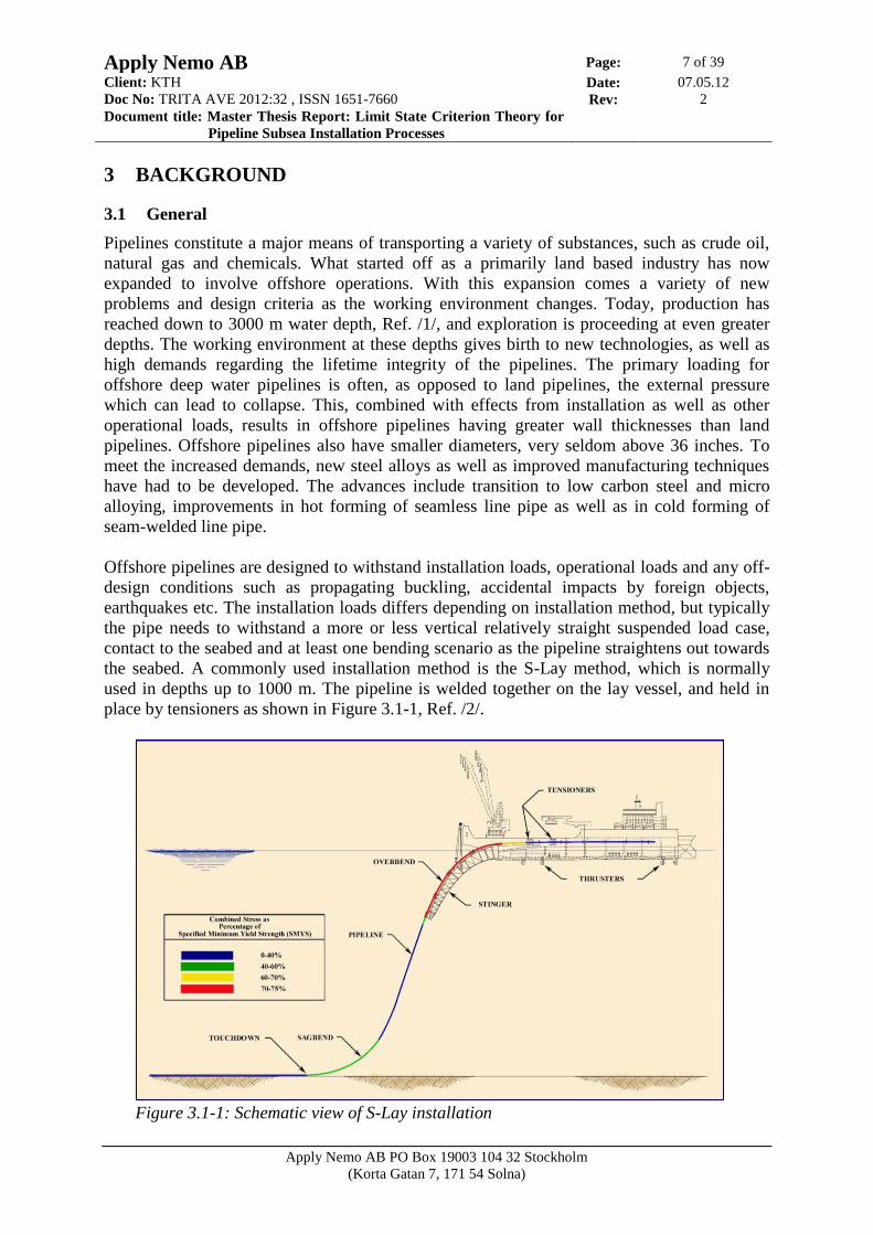
used in depths up to 1000 m. The pipeline is welded together on the lay vessel, and held in
place by tensioners as shown in Figure 3.1-1, Ref. /2/.
Figure 3.1-1: Schematic view of S-Lay installation
Apply Nemo AB Page: 8 of 39
Client: KTH Date: 07.05.12
Doc No: TRITA AVE 2012:32 , ISSN 1651-7660 Rev: 2
Document title: Master Thesis Report: Limit State Criterion Theory for
Pipeline Subsea Installation Processes
Apply Nemo AB PO Box 19003 104 32 Stockholm
(Korta Gatan 7, 171 54 Solna)
The vessel moves slowly forward and the pipe line is continuously welded together on the lay
vessel. As the vessel moves, the pipeline enters the boom-like curved stinger. The stinger is
open-framed, and supports the pipeline on v-shaped rollers. The section of the pipe on the
stinger is known as the overbend. As the vessel moves even further ahead, more pipe line is
welded together and the pipe forms into the S-shape illustrated in Figure 3.1-1. The curved
section closest to the seabed is called the sagbend.
The majority of the loading conditions both during installation and operation are not fully
covered by traditional stress-based design. Instead, the offshore pipeline industry performs
design with regard to so called limit states. Plastic deformation is often allowed, as long as the
structure is not close to excessive deformation or failure as defined by so called limit states.
Offshore pipeline projects are very costly, and it is of great interest for oil and gas companies
to reduce both manufacturing and installation costs as well as designing pipelines with
sufficient redundancy to reduce operation-based damages. Installation costs are in the order of
millions of NOK per day of operation and manufacturing costs are in the same order.
Reducing risks by ensuring that designs are correct are of high importance in the project, and
standards such as Ref. /3/ have been developed for this aim.
The oil and gas industry has its roots in the USA, and as a result the terminology and
definitions across the globe follow that of the American Petroleum Institute. Ref. /4/
3.2 Why this study
In pipeline design the pipeline wall thickness has to be calculated and determined by several
design checks. Apply Nemo is currently using Pipeline Engineering Tool (PET), a program
developed by DNV to perform OS-F101 ( Ref. /5/) design checks. The software is outdated as
there is currently a new revision of the DNV standard, Ref. /3/. PET works much like a “black
box” where the user supplies input data and gets minimum wall thicknesses of the pipe as
result without seeing intermediate steps explained in much detail. As the calculations done in
PET are used as input- and reference data in later stages of pipeline engineering projects, a
better understanding of all intermediate steps in wall thickness calculations is desired by
Apply Nemo. Also, tools for design checks shall be developed where needed to meet DNV-
OS-F101 2010 criteria.
3.3 What is done
The aim of this report is to present parts of the PET software in detail, showing all
calculations and intermediate steps and what parameters influence the results. A static FE-
analysis of the installation process is also done as validation of the S-Lay theory.
A Mathcad arc based on Ref. /3/ is made. Analytical results from the arc for the internal
pressure (bursting) limit state, external pressure (collapse) limit state, propagating buckling
limit state and the S-lay installation technique are compared and matched to correspondent
calculations made in PET. A FE-model of a pipeline is made and contact conditions for the
stinger and the seabed are added to simulate an S-lay installation process. The results from the
FE-analysis are compared to the analytical results from both the Mathcad arc and PET.
Changes between Ref. /5/ to Ref. /3/ are noted.
Apply Nemo AB Page: 9 of 39
Client: KTH Date: 07.05.12
Doc No: TRITA AVE 2012:32 , ISSN 1651-7660 Rev: 2
Document title: Master Thesis Report: Limit State Criterion Theory for
Pipeline Subsea Installation Processes
Apply Nemo AB PO Box 19003 104 32 Stockholm
(Korta Gatan 7, 171 54 Solna)
4 DESIGN BASIS
4.1 General
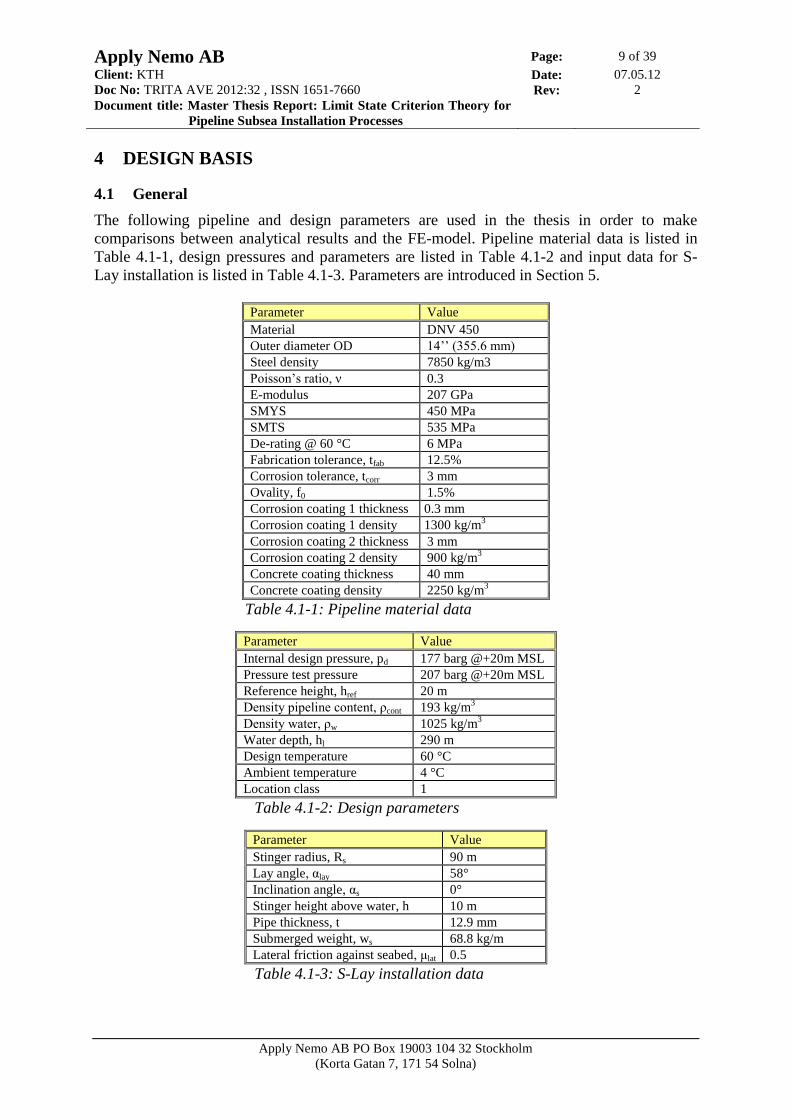
The following pipeline and design parameters are used in the thesis in order to make
comparisons between analytical results and the FE-model. Pipeline material data is listed in
Table 4.1-1, design pressures and parameters are listed in Table 4.1-2 and input data for S-
Lay installation is listed in Table 4.1-3. Parameters are introduced in Section 5.
Parameter Value
Material DNV 450
Outer diameter OD 14’’ (355.6 mm)
Steel density 7850 kg/m3
Poisson’s ratio, ν 0.3
E-modulus 207 GPa
SMYS 450 MPa
SMTS 535 MPa
De-rating @ 60 °C 6 MPa
Fabrication tolerance, tfab 12.5%
Corrosion tolerance, tcorr 3 mm
Ovality, f0 1.5%
Corrosion coating 1 thickness 0.3 mm
Corrosion coating 1 density 1300 kg/m3
Corrosion coating 2 thickness 3 mm
Corrosion coating 2 density 900 kg/m3
Concrete coating thickness 40 mm
Concrete coating density 2250 kg/m3
Table 4.1-1: Pipeline material data
Parameter Value
Internal design pressure, pd 177 barg @+20m MSL
Pressure test pressure 207 barg @+20m MSL
Reference height, href 20 m
Density pipeline content, ρcont 193 kg/m3
Density water, ρw 1025 kg/m3
Water depth, hl 290 m
Design temperature 60 °C
Ambient temperature 4 °C
Location class 1
Table 4.1-2: Design parameters
Parameter Value
Stinger radius, Rs 90 m
Lay angle, αlay 58°
Inclination angle, αs 0°
Stinger height above water, h 10 m
Pipe thickness, t 12.9 mm
Submerged weight, ws 68.8 kg/m
Lateral friction against seabed, μlat 0.5
Table 4.1-3: S-Lay installation data
Apply Nemo AB Page: 10 of 39
Client: KTH Date: 07.05.12
Doc No: TRITA AVE 2012:32 , ISSN 1651-7660 Rev: 2
Document title: Master Thesis Report: Limit State Criterion Theory for
Pipeline Subsea Installation Processes
Apply Nemo AB PO Box 19003 104 32 Stockholm
(Korta Gatan 7, 171 54 Solna)
5 ANALYTICAL METHODOLOGY
5.1 General
In this section the theory behind three limit state criteria are presented; bursting (with system
test), collapse/local buckling and propagating buckling. The analytical methodology for the S-
Lay installation method is also presented. At the end of each sub-section, notable changes
from Ref. /5/ to Ref. /3/ are made. The nomenclature, glossaries and symbol naming follows
Ref. /3/. Some terminology in the following sections is as follows:
Bursting - When a pipe ruptures due to high internal pressure
Collapse/Local buckling - When a pipe folds in on itself due to high external pressure
Design pressure - Maximum pressure a pressure protection system requires in order
to ensure that incidental pressure is not exceeded with sufficient
reliability
Incidental pressure - Maximum pressure the submarine pipeline system is designed for
Local pressure - Pressure conditions at water depth hl
Propagating buckling - A local buckle that propagates through the length of the pipe
Reference elevation - Height from sea level at which both system test pressure and
normal operation design pressure is given
Safety class - A classification based on potential failure consequence. Can be
Low/Medium/High
System test pressure - The pressure at which the complete submarine system is tested
prior commissioning. Shall satisfy the limit state for safety class
low.
Two different definitions of characteristic wall thickness are used in limit state theory; t1 and
t2. These are defined in Table 5.1-1.
Prior to operation
1) Operation
2)
t1 t-tfab t-tfab-tcorr
t2 t t-tcorr 1)
Is intended when there is negligible corrosion, e.g.
installation and system pressure test 2)
Is intended when there is corrosion
Table 5.1-1: Characteristic wall thickness
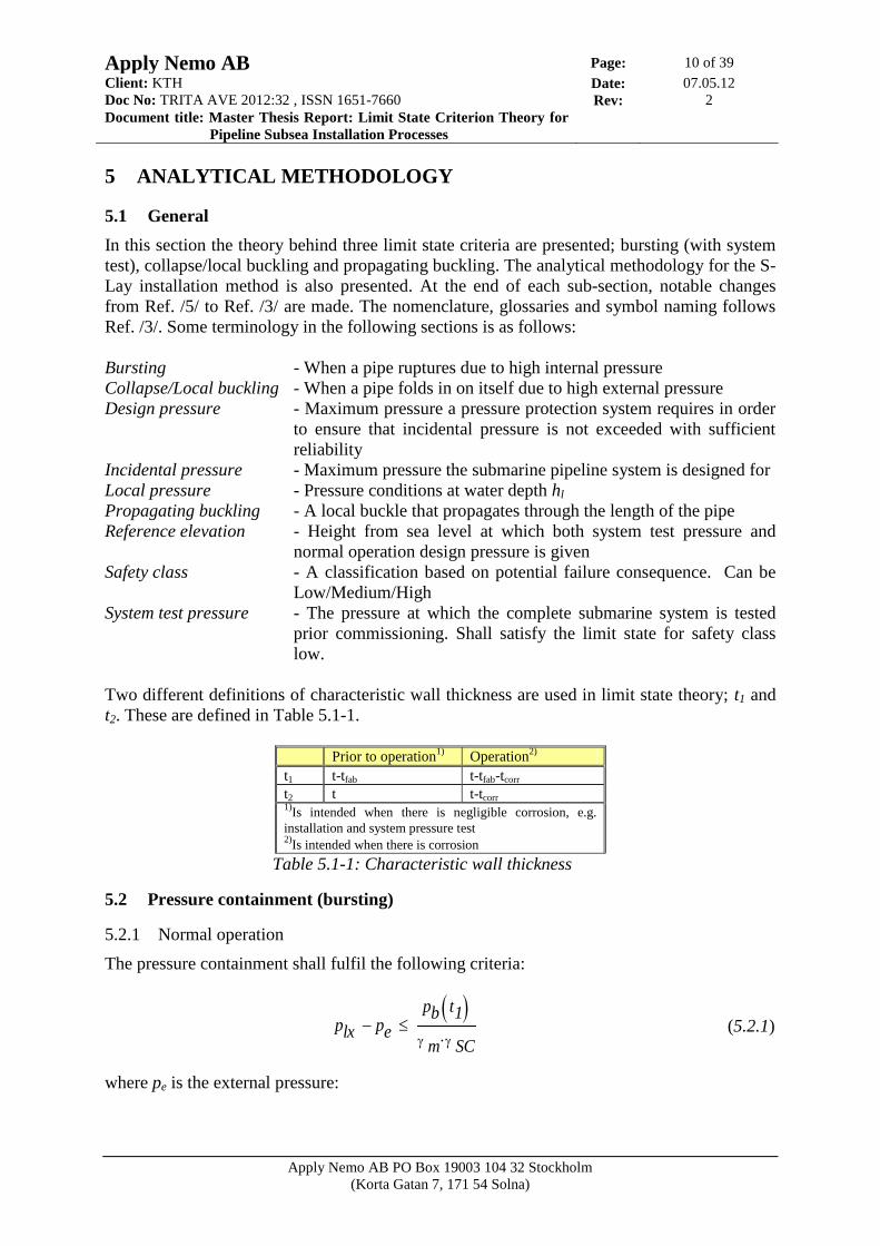
5.2 Pressure containment (bursting)
5.2.1 Normal operation
The pressure containment shall fulfil the following criteria:
(5.2.1)
where pe is the external pressure:
plx pepb t1 m SC
Apply Nemo AB Page: 11 of 39
Client: KTH Date: 07.05.12
Doc No: TRITA AVE 2012:32 , ISSN 1651-7660 Rev: 2
Document title: Master Thesis Report: Limit State Criterion Theory for
Pipeline Subsea Installation Processes
Apply Nemo AB PO Box 19003 104 32 Stockholm
(Korta Gatan 7, 171 54 Solna)
(5.2.2)
and plx = pli is the local incidental pressure during operation, γm is the material resistance
factor, γSC the safety class resistance factor, ρw the water density and hl the water depth. The
pressure containment resistance pb(t1) is given by:
.
(5.2.3)
Here, t1 is the wall thickness after having taken fabrication tolerances (tfab) and corrosion
tolerances (tcorr) into account, OD is the nominal outside diameter and fcb is the function
. (5.2.4)
The characteristic material yield stress, fy, and tensile strength, fu, are defined as:
(5.2.5)
(5.2.6)
where SMYS is the Specified Minimum Yield Strength, SMTS the Specified Minimum
Tensile Strength, fytemp and futemp the de-rating values due to temperature of yield stress and
tensile strength respectively and αU is the material strength factor.
For normal operation, plx = pli is the local incidental pressure given by:
(5.2.7)
where ρcont is the density of the relevant content of the pipeline, g the gravity, href the elevation
of the reference point (elevation positive upwards from the sea level) and hl the elevation of
the local pressure point (elevation positive upwards). For underwater operation, hl is the water
depth at which the pipeline is situated. Typically, the incidental pressure pinc is set to be 10%
higher than the design pressure pd, that is:
(5.2.8)
where γinc is the incidental to design pressure ratio, 1.10 for a typical pipeline system.
The outside diameter is expressed as:
(5.2.9)
pe w g hl
pb t1 2t1
OD t1fcb
2
3
fcb min fy
fu
1.15
fy SMYS fytemp U
fu SMTS futemp U
pli pinc cont g href hl
pinc pd inc
OD ID 2t
Apply Nemo AB Page: 12 of 39
Client: KTH Date: 07.05.12
Doc No: TRITA AVE 2012:32 , ISSN 1651-7660 Rev: 2
Document title: Master Thesis Report: Limit State Criterion Theory for
Pipeline Subsea Installation Processes
Apply Nemo AB PO Box 19003 104 32 Stockholm
(Korta Gatan 7, 171 54 Solna)
where ID is the inner diameter and t is the nominal wall thickness. The wall thickness t1 used
in equation (5.2.3) can be expressed as:
(5.2.10)
where tfab is the fabrication tolerance input either as a set value in millimetres or as a
percentage of the final nominal thickness.
Equation (5.2.3) is solved iteratively for increasing t until condition (5.2.1) is fulfilled.
5.2.2 System pressure test
During the system pressure test, safety class low shall be satisfied. The incidental to design
pressure ratio, γinc, shall be set to 1.0. The corrosion tolerance tcorr shall be set to zero. The
local system test pressure plt shall be used as plx in Equation (5.2.1) and can be expressed as:
(5.2.11)
where pt is the system test reference pressure at its reference elevation href and ρt the density
of the relevant test medium. The local system test pressure at reference level for safety class
low must fulfil the following requirement:
As for the case of normal operation, equation (5.2.3) is solved iteratively for increasing t until
condition (5.2.1) is fulfilled.
5.2.3 Changes from Ref. /5/ to Ref. /3/
No notable changes between the two standards regarding bursting limit state were observed.
5.3 Collapse/Local buckling
5.3.1 Normal operation
The external pressure at any point along the pipeline shall fulfil the following system collapse
criterion:
(5.3.1)
where pmin is the minimum relative internal pressure that can be sustained in the pipeline,
typically 0 bar gauge. The characteristic collapse pressure, pc(t1), is calculated as:
(5.3.2)
t1 t tfab tcorr
plt pt t g hreft hl
pe pminpc t1 m SC
pc t1 pel t1 pc t1 2
pp t1 2
pc t1 pel t1 pp t1 f0OD
t1
(5.2.12) plt h 0( ) pt 1.03pli
Apply Nemo AB Page: 13 of 39
Client: KTH Date: 07.05.12
Doc No: TRITA AVE 2012:32 , ISSN 1651-7660 Rev: 2
Document title: Master Thesis Report: Limit State Criterion Theory for
Pipeline Subsea Installation Processes
Apply Nemo AB PO Box 19003 104 32 Stockholm
(Korta Gatan 7, 171 54 Solna)
Here, f0 is the ovality factor. The elastic collapse pressure and the plastic collapse pressure can
be expressed, respectively, as:
(5.3.3)
(5.3.4)
where E is Young’s modulus, ν Poisson’s ratio and αfab the fabrication factor. The analytical
solution to equation (5.3.2) is presented in equations (5.3.5) to (5.3.12):
(5.3.5)
(5.3.6)
(5.3.7)
(5.3.8)
(5.3.9)
(5.3.10)
(5.3.11)
(5.3.12)
The above equations are solved iteratively for increasing t until condition (5.3.1) is fulfilled.
5.3.2 Changes from Ref. /5/ to Ref. /3/
The limit state criterion for collapse/local buckling is changed from
(5.3.13)
to
(5.3.14)
In the old standard, a note is made that “…internal pressure may be taken into account
provided that it can be continuously sustained”, thus accounting for pmin. The factor of 1.1 is
pel 2
Et1
OD
3
1 2
pp fy fab 2t1
OD
pc y1
3b
b pel
c pp2
pp pel f0OD
t1
d pel pp2
u1
3
1
3b
2 c
v1
2
2
27b
3
1
3b c d
acosv
u3
y 2 u cos
360
180
pe
pc
1.1 m SC
pe pminpc t1 m SC
Apply Nemo AB Page: 14 of 39
Client: KTH Date: 07.05.12
Doc No: TRITA AVE 2012:32 , ISSN 1651-7660 Rev: 2
Document title: Master Thesis Report: Limit State Criterion Theory for
Pipeline Subsea Installation Processes
Apply Nemo AB PO Box 19003 104 32 Stockholm
(Korta Gatan 7, 171 54 Solna)
removed from the denominator. The characteristic collapse pressure pc is in the old standard
calculated using wall thickness t2, which does not include fabrication tolerances. In the new
standard, thickness t1 is used together with a guidance note stating that t1 is normally
representative of a pipeline’s weakest point but for seamless produced pipelines, a larger
thickness between t1 and t2 may be used.
5.4 Propagating buckling
5.4.1 Normal operation
Propagating buckling cannot be initiated unless local buckling has occurred. The propagating
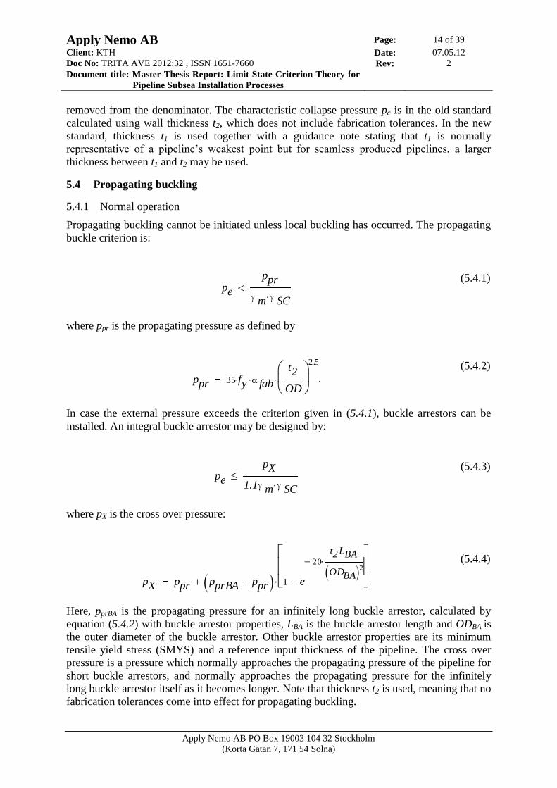
buckle criterion is:
(5.4.1)
where ppr is the propagating pressure as defined by
.
(5.4.2)
In case the external pressure exceeds the criterion given in (5.4.1), buckle arrestors can be
installed. An integral buckle arrestor may be designed by:
(5.4.3)
where pX is the cross over pressure:
.
(5.4.4)
Here, pprBA is the propagating pressure for an infinitely long buckle arrestor, calculated by
equation (5.4.2) with buckle arrestor properties, LBA is the buckle arrestor length and ODBA is
the outer diameter of the buckle arrestor. Other buckle arrestor properties are its minimum
tensile yield stress (SMYS) and a reference input thickness of the pipeline. The cross over
pressure is a pressure which normally approaches the propagating pressure of the pipeline for
short buckle arrestors, and normally approaches the propagating pressure for the infinitely
long buckle arrestor itself as it becomes longer. Note that thickness t2 is used, meaning that no
fabrication tolerances come into effect for propagating buckling.
pe
ppr
m SC
ppr 35 fy fabt2
OD
2.5
pe
pX
1.1 m SC
pX ppr pprBA ppr 1 e
20t2 LBA
ODBA 2
Apply Nemo AB Page: 15 of 39
Client: KTH Date: 07.05.12
Doc No: TRITA AVE 2012:32 , ISSN 1651-7660 Rev: 2
Document title: Master Thesis Report: Limit State Criterion Theory for
Pipeline Subsea Installation Processes
Apply Nemo AB PO Box 19003 104 32 Stockholm
(Korta Gatan 7, 171 54 Solna)
5.4.2 Changed from Ref. /5/ to Ref. /3/
In the old standard, no separate design criterion is given for buckle arrestors and pX is subject
to the same criterion as ppr is in equation (5.4.1). In the new standard, the design criterion
(5.4.3) with a safety factor of 1.1 is given.
In the old standard, a note is made that discussion about buckle arrestors and propagating
pressure is made in Sriskandarajah (1987), also cited in Ref. /6/. In the new standard, equation
(5.4.4) is given as well as a note that the equation is taken from Torselletti et al. In equation
(5.4.4) the constant in the exponent, -20, is changed from -15.
5.5 S-Lay
5.5.1 General
The pipe is considered from where it leaves the barge and enters the stinger above water with
an inclination angle. The pipe is assumed to be in full contact with the stinger until it departs
at the inflection point. From here, the pipe is assumed to follow a catenary shape until it
touches the seabed.
A utilization ratio design check is made for both the overbend and the sagbend. At the stinger,
the check is performed according to a displacement controlled condition. At the sagbend, the
check is performed according to a load controlled condition. For both cases, load case “a” in
Ref. /3/ is used.
5.5.2 Catenary theory
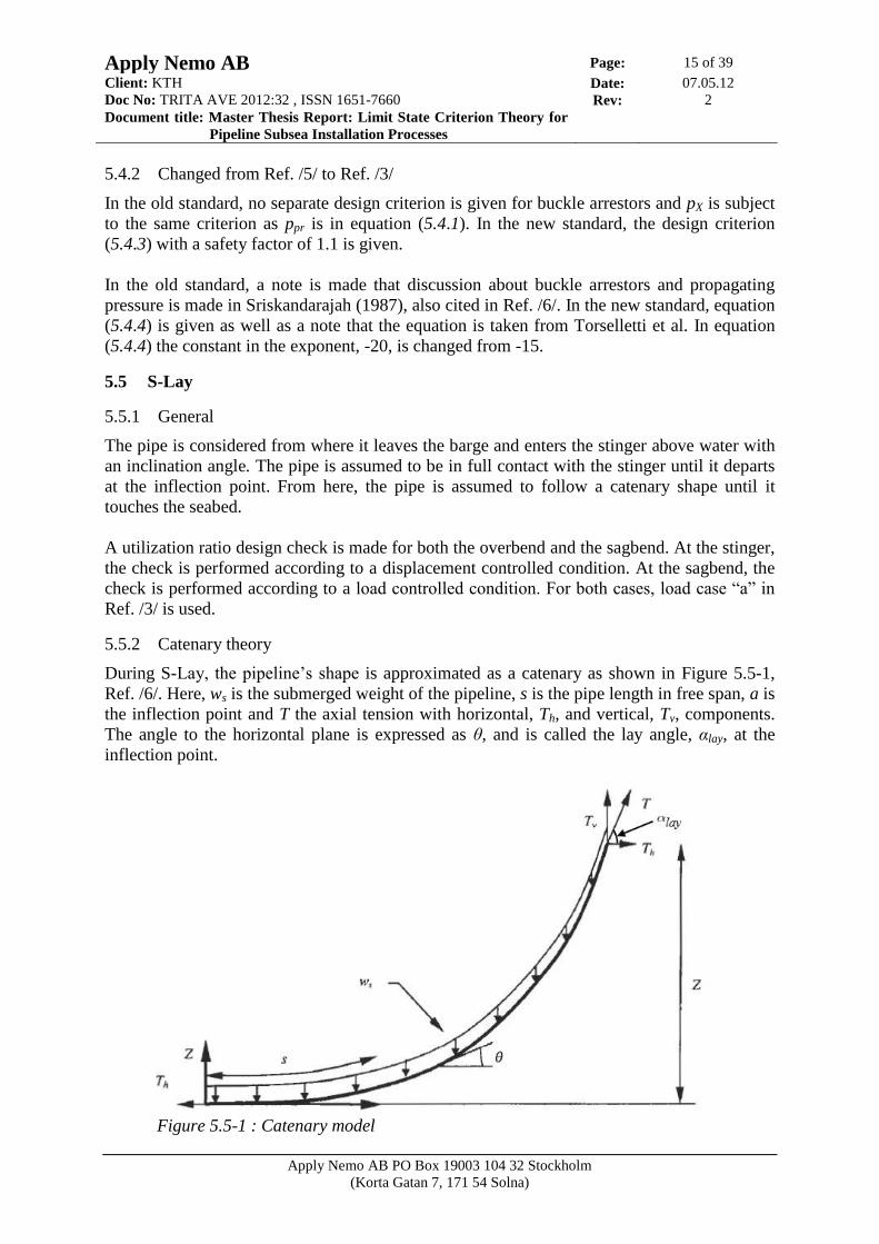
During S-Lay, the pipeline’s shape is approximated as a catenary as shown in Figure 5.5-1,
Ref. /6/. Here, ws is the submerged weight of the pipeline, s is the pipe length in free span, a is
the inflection point and T the axial tension with horizontal, Th, and vertical, Tv, components.
The angle to the horizontal plane is expressed as θ, and is called the lay angle, αlay, at the
inflection point.
Figure 5.5-1 : Catenary model
Apply Nemo AB Page: 16 of 39
Client: KTH Date: 07.05.12
Doc No: TRITA AVE 2012:32 , ISSN 1651-7660 Rev: 2
Document title: Master Thesis Report: Limit State Criterion Theory for
Pipeline Subsea Installation Processes
Apply Nemo AB PO Box 19003 104 32 Stockholm
(Korta Gatan 7, 171 54 Solna)
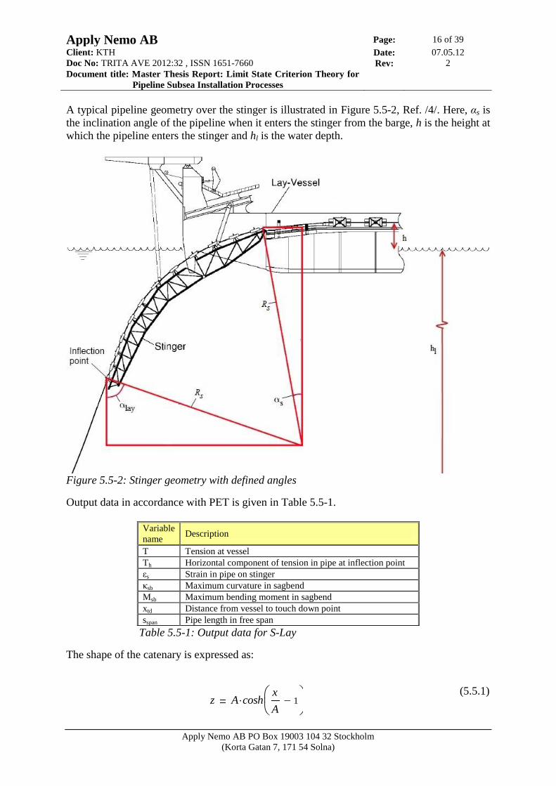
A typical pipeline geometry over the stinger is illustrated in Figure 5.5-2, Ref. /4/. Here, αs is
the inclination angle of the pipeline when it enters the stinger from the barge, h is the height at
which the pipeline enters the stinger and hl is the water depth.
Figure 5.5-2: Stinger geometry with defined angles
Output data in accordance with PET is given in Table 5.5-1.
Variable
name Description
T Tension at vessel
Th Horizontal component of tension in pipe at inflection point
εs Strain in pipe on stinger
κsb Maximum curvature in sagbend
Msb Maximum bending moment in sagbend
xtd Distance from vessel to touch down point
sspan Pipe length in free span
Table 5.5-1: Output data for S-Lay
The shape of the catenary is expressed as:
(5.5.1)
z A coshx
A1
Apply Nemo AB Page: 17 of 39
Client: KTH Date: 07.05.12
Doc No: TRITA AVE 2012:32 , ISSN 1651-7660 Rev: 2
Document title: Master Thesis Report: Limit State Criterion Theory for
Pipeline Subsea Installation Processes
Apply Nemo AB PO Box 19003 104 32 Stockholm
(Korta Gatan 7, 171 54 Solna)
where
(5.5.2)
In this equation, A can be interpreted as the radius of the curve in the sagbend at the touch
down point. The submerged weight, ws, can be calculated as
(5.5.3)
where ρsteel is the pipeline steel density and ρw is the water density. If the pipeline is coated
with corrosion resistant material and/or concrete coating, the weight of these coatings is
included in the calculation as well. The distance from the inflection point and the touch down
point in the catenary solution is
(5.5.4)
where hmod is the vertical distance between the seabed and the inflection point:
(5.5.5)
Here, hl is the water depth, h is the stinger height above water, Rs is the stinger radius, αs the
inclination angle and αlay the lay angle. The pipe length in free span is expressed as
(5.5.6)
The horizontal component of the axial tension in the pipeline, Th, can be expressed for θ=αlay
and z=hmod as
(5.5.7)
The vertical component of the tension at the inflection point is
(5.5.8)
The tension parallel to the pipe at the lay vessel is thus the sum of the tension at the inflection
point and the weight component parallel to the stinger of the pipe on the stinger:
(5.5.9)
ATh
ws
ws steel w OD
2OD t( )
2
2
xtd A acoshhmod A
A
hmod hl h Rs cos s cos lay
sspan hmod 1 2A
hmod
Th
hmod ws
tan lay 2
1 1 tan lay 2
Tv ws sspan
T Tv2
Th2
ws Rs cos s cos lay
Apply Nemo AB Page: 18 of 39
Client: KTH Date: 07.05.12
Doc No: TRITA AVE 2012:32 , ISSN 1651-7660 Rev: 2
Document title: Master Thesis Report: Limit State Criterion Theory for
Pipeline Subsea Installation Processes
Apply Nemo AB PO Box 19003 104 32 Stockholm
(Korta Gatan 7, 171 54 Solna)
The maximum curvature is found at the touch down point:
(5.5.10)
From this, the maximum bending moment on the pipe can be found as:
(5.5.11)
where EI is the bending stiffness of the pipe. The minimum horizontal lay radius can be
expressed as:
(5.5.12)
where μlat is the lateral coefficient of friction towards the seabed. The bending strain of the
pipe on the stinger is
(5.5.13)
The axial tensile strain of the pipe on the stinger may be significant (~10% of εs) in deep
waters but is in this study neglected.
5.5.3 Utilisation ratio at stinger
The input parameters used for the displacement controlled condition design check are
presented in Table 5.5-2.
Parameter Value
Corrosion allowance, tcorr 0 mm
Material derating 0 MPa
Internal pressure, pi 0 bar
External pressure, pe 0 bar
Functional compressive strain, εF εs
Environmental compressive strain, εE 0.0
Load condition factor, γC 1.00
Safety Class LOW
Table 5.5-2: Input parameters for displacement
controlled condition design check
Pipe members subjected to longitudinal compressive strain and internal overpressure shall be
designed to satisfy the following criterion at all cross sections:
sb1
A
Msb sb EI
Rlay
Th
lat ws
sOD
2 Rs OD
Apply Nemo AB Page: 19 of 39
Client: KTH Date: 07.05.12
Doc No: TRITA AVE 2012:32 , ISSN 1651-7660 Rev: 2
Document title: Master Thesis Report: Limit State Criterion Theory for
Pipeline Subsea Installation Processes
Apply Nemo AB PO Box 19003 104 32 Stockholm
(Korta Gatan 7, 171 54 Solna)
for (5.5.14)
(5.5.15)
where εSd is the design compressive strain, εF is the functional compressive strain, γF and γE
are functional and environmental load effect factors respectively, γC the load condition factor,
εE the environmental compressive strain and εRd is the design resistance strain:
(5.5.16)
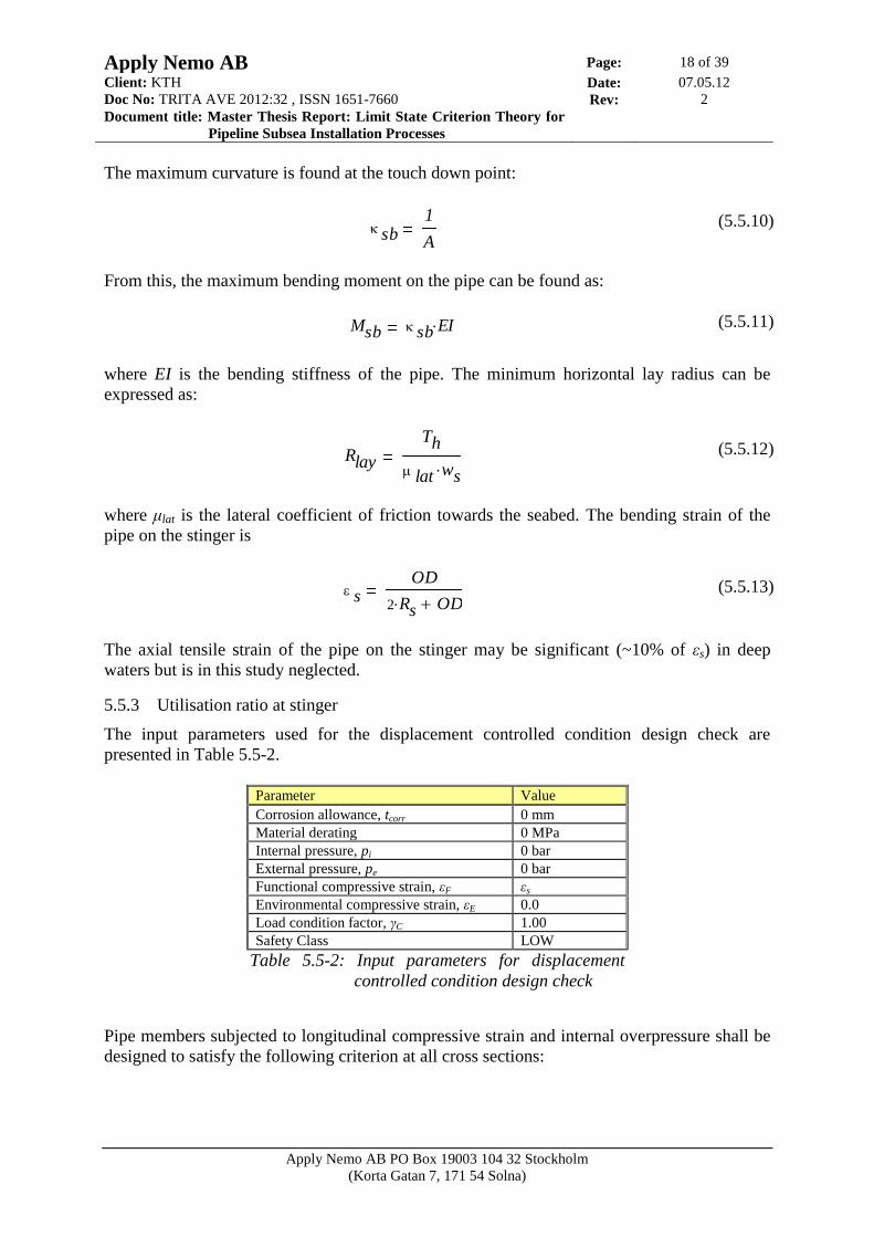
Here, γε is the resistance strain factor and εc the characteristic bending strain resistance:
(5.5.17)
where the pressure containment resistance pb(t) is defined in (5.2.3), αh is the minimum strain
hardening and αgw is the girth weld factor as defined in Figure 5.5-3. Wall thickness t2 is used;
that is, no fabrication tolerances are included. Note that as both pmin and pe are zero for the
design check, the second parenthesis in (5.5.17) equals 1.
Figure 5.5-3: Girth weld factor, valid for 20<D/t<60
5.5.4 Utilisation ratio in sagbend
The input parameters used for the load controlled condition design check are presented in
Table 5.5-3.
Sd
Rd
1D
t2
45 pi pe
Sd F F C E E
Rd
c
c 0.78
t2
OD0.01
1 5.75
pmin pe
pb t2
h1.5
gw
Apply Nemo AB Page: 20 of 39
Client: KTH Date: 07.05.12
Doc No: TRITA AVE 2012:32 , ISSN 1651-7660 Rev: 2
Document title: Master Thesis Report: Limit State Criterion Theory for
Pipeline Subsea Installation Processes
Apply Nemo AB PO Box 19003 104 32 Stockholm
(Korta Gatan 7, 171 54 Solna)
Parameter Value
Corrosion allowance, tcorr 0 mm
Material derating 0 MPa
Internal pressure, pi 0 bar
External pressure, pe ρw∙g∙hl bar
Functional bending moment, MF Msb
Environmental bending moment, ME 0.0
Functional effective axial force, SF Th
Environmental effective axial force, SE 0.0
Load effect factor, γC 1.0
Safety Class LOW
Table 5.5-3: Input parameters for displacement
controlled condition design check.
Pipe members subjected to bending moment, effective axial force and external overpressure
shall be designed to satisfy the following criterion at all cross sections:
(5.5.18)
where MSd is the design moment as given in equation (5.5.19), αc the flow stress parameter as
per equation (5.5.20) and Mp the plastic moment capacity as defined in equation (5.5.22). The
plastic force capacity Sp and the design effective axial force SSd are defined in equations
(5.5.23) and (5.5.24), and the characteristic collapse pressure pc(t2) is derived in equations
(5.3.2)-(5.3.12). The design moment MSd is defined using the functional and environmental
bending moments MF and ME.
(5.5.19)
The flow stress parameter is defined as:
(5.5.20)
where β is:
(5.5.21)
m SCMSd
c Mp t2
m SC SSd
c Sp t2
2
2
m SCpe pmin
pc t2
2
1
MSd MF F C ME E
c 1 ( )
fu
fy
0.5OD
t2
15if
60OD
t2
9015
OD
t2
60if
0OD
t2
60if
Apply Nemo AB Page: 21 of 39
Client: KTH Date: 07.05.12
Doc No: TRITA AVE 2012:32 , ISSN 1651-7660 Rev: 2
Document title: Master Thesis Report: Limit State Criterion Theory for
Pipeline Subsea Installation Processes
Apply Nemo AB PO Box 19003 104 32 Stockholm
(Korta Gatan 7, 171 54 Solna)
The tensile strength fu in (5.5.20) is in axial direction, and should therefore reduced by 5%.
The plastic capacities for a pipe are defined by:
(5.5.22)
(5.5.23)
The design effective axial force is defined using the functional and environmental axial forces
SF and SE.
(5.5.24)
5.5.5 Changes from Ref. /5/ to Ref. /3/
The yield stress definition is changed from
(5.5.25)
to
, (5.5.26)
Thus removing the anisotropy factor αA. A note is however made that in case of longitudinal
loading, a minimum tensile strength 5% less than the required value is acceptable.
The hardening factor αh for the material SMYS450 is changed from 0.92 to 0.93. The
definition of the load controlled condition is changed from
(5.5.27)
to
(5.5.28)
moving the factors γm and γSC inside the parenthesis and adding the effect of pmin.
The definition of the coefficient β is changed from (5.5.29) to (5.5.21).
Mp t( ) fy OD t( )2
t
Sp t( ) fy OD t( ) t
SSd SF F C SE E
fy SMYS fytemp U A
fy SMYS fytemp U
m SCMSd
c Mp t2 m SC
SSd
c Sp t2
2
2
m SCpe
pc t2
2
1
m SCMSd
c Mp t2
m SC SSd
c Sp t2
2
2
m SCpe pmin
pc t2
2
1
Apply Nemo AB Page: 22 of 39
Client: KTH Date: 07.05.12
Doc No: TRITA AVE 2012:32 , ISSN 1651-7660 Rev: 2
Document title: Master Thesis Report: Limit State Criterion Theory for
Pipeline Subsea Installation Processes
Apply Nemo AB PO Box 19003 104 32 Stockholm
(Korta Gatan 7, 171 54 Solna)
(5.5.29)
where
for (5.5.30)
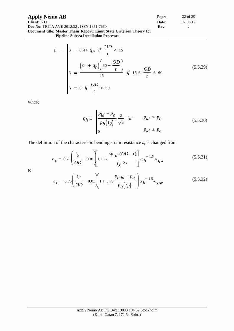
The definition of the characteristic bending strain resistance εc is changed from
(5.5.31)
to
(5.5.32)
0.4 qhOD
t15if
0.4 qh 60OD
t
4515
OD
t 60if
0OD
t60if
qh
pld pe
pb t2 2
3
0
c 0.78
t2
OD0.01
1 5
p d OD t( )
fy 2 t
h1.5
gw
c 0.78
t2
OD0.01
1 5.75
pmin pe
pb t2
h1.5
gw
pld pe
pld pe
Apply Nemo AB Page: 23 of 39
Client: KTH Date: 07.05.12
Doc No: TRITA AVE 2012:32 , ISSN 1651-7660 Rev: 2
Document title: Master Thesis Report: Limit State Criterion Theory for
Pipeline Subsea Installation Processes
Apply Nemo AB PO Box 19003 104 32 Stockholm
(Korta Gatan 7, 171 54 Solna)
6 FINITE ELEMENT MODELLING
6.1 S-Lay installation global model
6.1.1 General
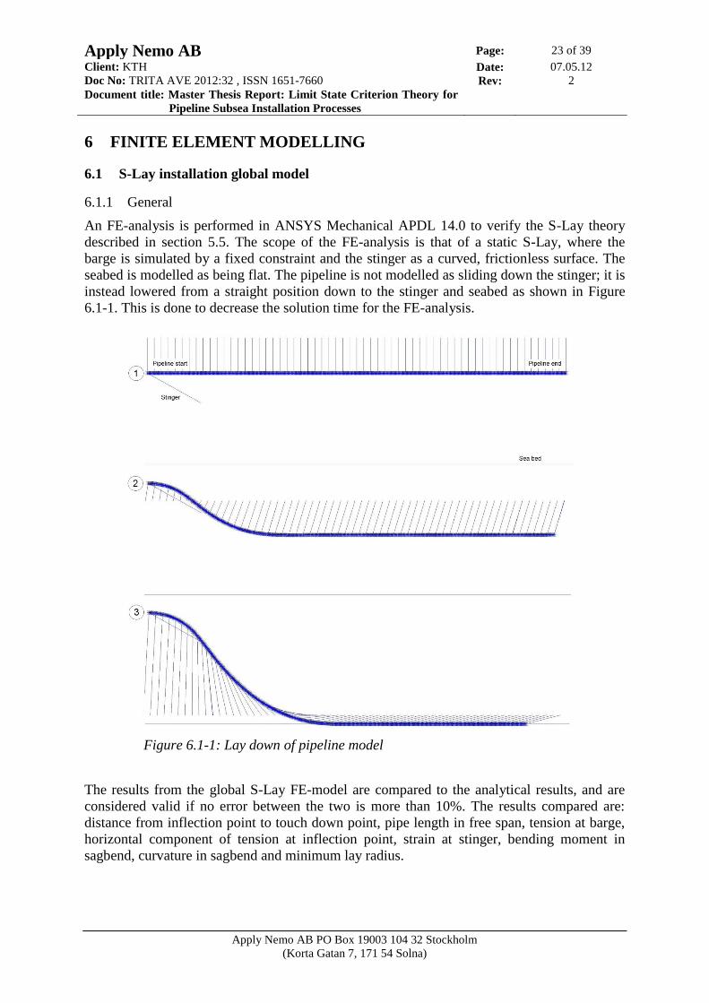
An FE-analysis is performed in ANSYS Mechanical APDL 14.0 to verify the S-Lay theory
described in section 5.5. The scope of the FE-analysis is that of a static S-Lay, where the
barge is simulated by a fixed constraint and the stinger as a curved, frictionless surface. The
seabed is modelled as being flat. The pipeline is not modelled as sliding down the stinger; it is
instead lowered from a straight position down to the stinger and seabed as shown in Figure
6.1-1. This is done to decrease the solution time for the FE-analysis.
Figure 6.1-1: Lay down of pipeline model
The results from the global S-Lay FE-model are compared to the analytical results, and are
considered valid if no error between the two is more than 10%. The results compared are:
distance from inflection point to touch down point, pipe length in free span, tension at barge,
horizontal component of tension at inflection point, strain at stinger, bending moment in
sagbend, curvature in sagbend and minimum lay radius.
Apply Nemo AB Page: 24 of 39
Client: KTH Date: 07.05.12
Doc No: TRITA AVE 2012:32 , ISSN 1651-7660 Rev: 2
Document title: Master Thesis Report: Limit State Criterion Theory for
Pipeline Subsea Installation Processes
Apply Nemo AB PO Box 19003 104 32 Stockholm
(Korta Gatan 7, 171 54 Solna)
6.1.2 Geometry and elements
A 1000 m long straight pipeline is modelled using 1 m PIPE288 elements, and is hung in
LINK180 elements which are only active in tension. The stinger is modelled using an 8-node
quadrilateral TARGE170 element, forming an arc with the stinger radius. The seabed is
modelled as flat, using a 4-node quadrilateral TARGE170 element. All nodes constituting the
pipe are covered by CONTA175 elements to enable isotropic friction contact between the
pipeline and the stinger and seabed respectively. The friction coefficient is 0.5. The set-up is
seen in the first picture of Figure 6.1-1. The elements used for the model, along with
keyoptions changed from their default value, are listed in Table 6.1-1.
Model component Element KEYOPT KEYOPT description
Pipeline PIPE288 KEYOPT(4)=2 Hoop strain treatment: Thick pipe
theory
KEYOPT(6)=0 Internal and external pressures cause
loads on end caps
KEYOPT(9)=1 Output control at integration points:
Maximum and minimum
stresses/strains
KEYOPT(11)=1 Output control for values
extrapolated to the element and
section nodes: Maximum and
minimum stresses/strains
Seabed TARGE170 -
Stinger TARGE170 -
Contact between stinger and pipeline CONTA175 KEYOPT(10)=2 Contact Stiffness Update: Each
iteration based on current mean
stress of underlying elements (pair
based).
Contact between stinger and seabed CONTA175 KEYOPT(10)=2 Contact Stiffness Update: Each
iteration based on current mean
stress of underlying elements (pair
based).
Supports used to lower pipeline LINK180 -
Table 6.1-1: ANSYS element types used and their respective KEYOPT() values, if changed
from their default values
6.1.3 Load steps and constraints
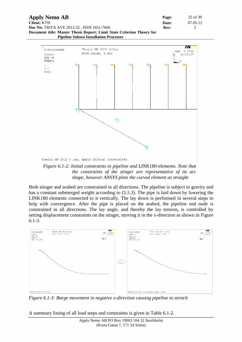
The pipeline start node is constrained in all directions as shown in Figure 6.1-2, simulating the
tensioners holding the pipe. The top nodes of the LINK180 elements are also constrained.
Apply Nemo AB Page: 25 of 39
Client: KTH Date: 07.05.12
Doc No: TRITA AVE 2012:32 , ISSN 1651-7660 Rev: 2
Document title: Master Thesis Report: Limit State Criterion Theory for
Pipeline Subsea Installation Processes
Apply Nemo AB PO Box 19003 104 32 Stockholm
(Korta Gatan 7, 171 54 Solna)
Figure 6.1-2: Initial constraints to pipeline and LINK180-elements. Note that
the constraints of the stinger are representative of its arc
shape, however ANSYS plots the curved element as straight
Both stinger and seabed are constrained in all directions. The pipeline is subject to gravity and
has a constant submerged weight according to (5.5.3). The pipe is laid down by lowering the
LINK180 elements connected to it vertically. The lay down is performed in several steps to
help with convergence. After the pipe is placed on the seabed, the pipeline end node is
constrained in all directions. The lay angle, and thereby the lay tension, is controlled by
setting displacement constraints on the stinger, moving it in the x-direction as shown in Figure
6.1-3.
Figure 6.1-3: Barge movement in negative x-direction causing pipeline to stretch
A summary listing of all load steps and constraints is given in Table 6.1-2.
Apply Nemo AB Page: 26 of 39
Client: KTH Date: 07.05.12
Doc No: TRITA AVE 2012:32 , ISSN 1651-7660 Rev: 2
Document title: Master Thesis Report: Limit State Criterion Theory for
Pipeline Subsea Installation Processes
Apply Nemo AB PO Box 19003 104 32 Stockholm
(Korta Gatan 7, 171 54 Solna)
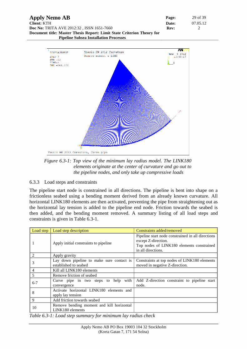
Load step Load step description Constraints added/removed
1 Apply initial constraints to pipeline
Pipeline start node (at stinger) constrained in all
directions.
Top nodes of LINK180 elements constrained in all
directions.
2 Apply gravity Delete pipeline start node constraint around Y-axis.
3-10 Lay down pipe. Done in several steps
to help with convergence
Constraints at top nodes of LINK180 elements
moved in negative Z-direction.
11 Apply constraints to pipeline end node Pipeline end node (at sea bed) constrained in all
directions.
12 Kill LINK180 elements holding pipe
13 Move stinger in x-direction Constraints at all stinger nodes as well as pipeline
start node moved in negative x-direction
Table 6.1-2: Load step and constraints summary for S-Lay
6.2 S-Lay installation submodel
6.2.1 General
The point in the sagbend where the maximum curvature and bending moment is observed is
of special interest, and a submodel of this section is made using solid-shell elements. Bending
moment and axial force is taken from the above global model at 12 m distance on both sides
from the point of interest. A pipeline model with finer mesh is made.
6.2.2 Geometry and elements
The pipeline in the sagbend submodel is made with the solid-shell element SOLSH190. A 24
m long straight pipeline is modelled with an element mesh of 0.05 x 0.02 x 0.0129 m
(LxBxH), where the height is the pipe thickness gotten from Table 4.1-3. Number of elements
in circumference is 40. All KEYOPTs are at their default values. The submodel is seen in
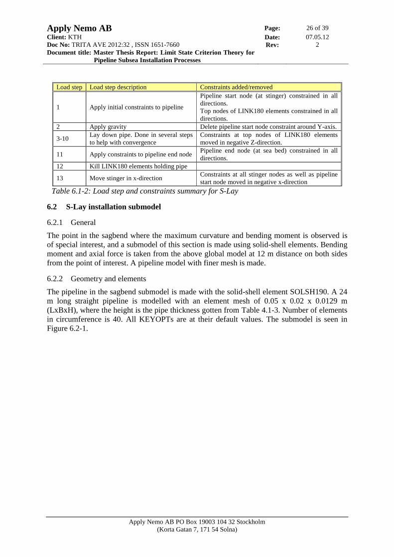
Figure 6.2-1.
Apply Nemo AB Page: 27 of 39
Client: KTH Date: 07.05.12
Doc No: TRITA AVE 2012:32 , ISSN 1651-7660 Rev: 2
Document title: Master Thesis Report: Limit State Criterion Theory for
Pipeline Subsea Installation Processes
Apply Nemo AB PO Box 19003 104 32 Stockholm
(Korta Gatan 7, 171 54 Solna)
Figure 6.2-1: Pipeline end showing the fine mesh of the submodel
6.2.3 Load steps and constraints
The submodel is solved using only one load step. All nodes at the pipeline start cross-section
are constrained in all directions. Nodes in the cross-section at the pipeline end are fixed so
that they cannot move sideways, i.e. in y-direction in Figure 6.2-1. The bending moment and
axial force from the global model is applied in the submodel. The bending moment is input as
a force couple, acting on the 6 o’clock node and the 12 o’clock node of the pipe end cross-
section. The axial force applied is divided evenly amongst the pipe end nodes, making the
sum equal that which is gotten from the global model.
Stresses at the pipe top and bottom are compared between the two models for verification,
together with a comparison of the deformation in the two models. The resulting stresses
throughout the pipe are taken as the mean value of the stresses at the two nodes comprising an
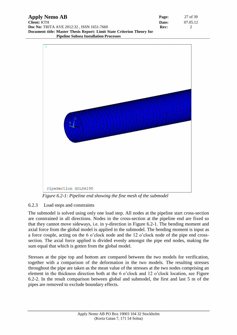
element in the thickness direction both at the 6 o’clock and 12 o’clock location, see Figure
6.2-2. In the result comparison between global and submodel, the first and last 5 m of the
pipes are removed to exclude boundary effects.
Apply Nemo AB Page: 28 of 39
Client: KTH Date: 07.05.12
Doc No: TRITA AVE 2012:32 , ISSN 1651-7660 Rev: 2
Document title: Master Thesis Report: Limit State Criterion Theory for
Pipeline Subsea Installation Processes
Apply Nemo AB PO Box 19003 104 32 Stockholm
(Korta Gatan 7, 171 54 Solna)
Figure 6.2-2: Cross-section of submodel pipeline with 6 o’clock and 12
o’clock nodes marked. Stresses at these nodes are averaged
respectively for comparison with global model
6.3 S-Lay installation minimum lay radius model
6.3.1 General
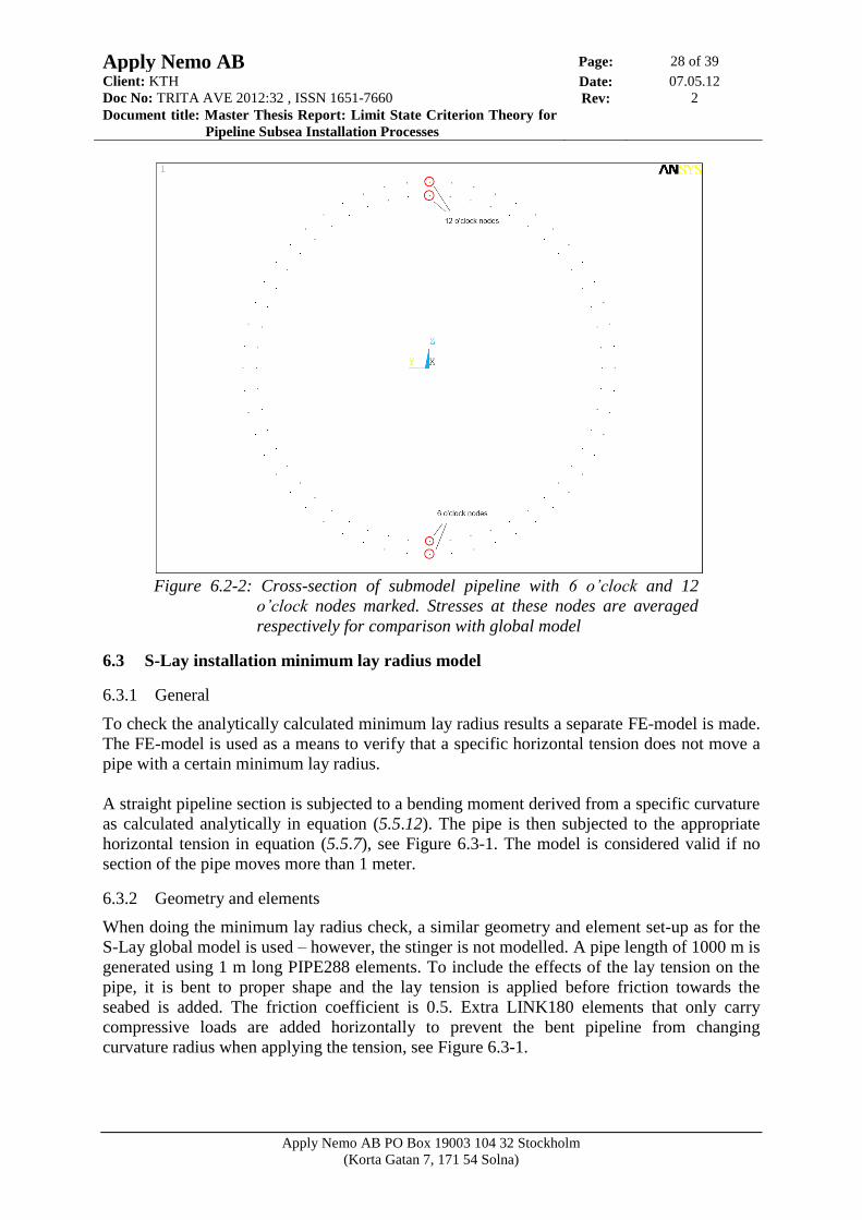
To check the analytically calculated minimum lay radius results a separate FE-model is made.
The FE-model is used as a means to verify that a specific horizontal tension does not move a
pipe with a certain minimum lay radius.
A straight pipeline section is subjected to a bending moment derived from a specific curvature
as calculated analytically in equation (5.5.12). The pipe is then subjected to the appropriate
horizontal tension in equation (5.5.7), see Figure 6.3-1. The model is considered valid if no
section of the pipe moves more than 1 meter.
6.3.2 Geometry and elements
When doing the minimum lay radius check, a similar geometry and element set-up as for the
S-Lay global model is used – however, the stinger is not modelled. A pipe length of 1000 m is
generated using 1 m long PIPE288 elements. To include the effects of the lay tension on the
pipe, it is bent to proper shape and the lay tension is applied before friction towards the
seabed is added. The friction coefficient is 0.5. Extra LINK180 elements that only carry
compressive loads are added horizontally to prevent the bent pipeline from changing
curvature radius when applying the tension, see Figure 6.3-1.
Apply Nemo AB Page: 29 of 39
Client: KTH Date: 07.05.12
Doc No: TRITA AVE 2012:32 , ISSN 1651-7660 Rev: 2
Document title: Master Thesis Report: Limit State Criterion Theory for
Pipeline Subsea Installation Processes
Apply Nemo AB PO Box 19003 104 32 Stockholm
(Korta Gatan 7, 171 54 Solna)
Figure 6.3-1: Top view of the minimum lay radius model. The LINK180
elements originate at the center of curvature and go out to
the pipeline nodes, and only take up compressive loads
6.3.3 Load steps and constraints
The pipeline start node is constrained in all directions. The pipeline is bent into shape on a
frictionless seabed using a bending moment derived from an already known curvature. All
horizontal LINK180 elements are then activated, preventing the pipe from straightening out as
the horizontal lay tension is added to the pipeline end node. Friction towards the seabed is
then added, and the bending moment removed. A summary listing of all load steps and
constraints is given in Table 6.3-1.
Load step Load step description Constraints added/removed
1 Apply initial constraints to pipeline
Pipeline start node constrained in all directions
except Z-direction.
Top nodes of LINK180 elements constrained
in all directions.
2 Apply gravity
3 Lay down pipeline to make sure contact is
established to seabed
Constraints at top nodes of LINK180 elements
moved in negative Z-direction.
4 Kill all LINK180 elements
5 Remove friction of seabed
6-7 Curve pipe in two steps to help with
convergence
Add Z-direction constraint to pipeline start
node.
8 Activate horizontal LINK180 elements and
apply lay tension
9 Add friction towards seabed
10 Remove bending moment and kill horizontal
LINK180 elements
Table 6.3-1: Load step summary for minimum lay radius check
Apply Nemo AB Page: 30 of 39
Client: KTH Date: 07.05.12
Doc No: TRITA AVE 2012:32 , ISSN 1651-7660 Rev: 2
Document title: Master Thesis Report: Limit State Criterion Theory for
Pipeline Subsea Installation Processes
Apply Nemo AB PO Box 19003 104 32 Stockholm
(Korta Gatan 7, 171 54 Solna)
7 RESULTS
7.1 Analytical results
Results for all limit states and installation methods are achieved using input data specified in
Section 4. Mathcad results are based on DNV-OS-F101 (2010) and PET results are based on
DNV-OS-F101 (2000). Input variables presented in the theory section but with values not
listed previously for this case are given in Table 7.1-1.
Variable Description Value
αh Hardening factor 0.93
αfab Fabrication factor 1
αU Material strength factor U 0.96
αgw Girth weld factor 0.924
Table 7.1-1: Additional input data
7.1.1 Bursting
Safety class for bursting is in this particular case Medium. Analytical results for bursting limit
state are presented in Table 7.1-2.
Bursting
Parameter Description Mathcad result PET result
t Required minimum wall thickness for normal operation 12.48 mm 12.49 mm
t Required minimum wall thickness for system pressure test 8.76 mm 8.77 mm
Table 7.1-2: Analytical results for bursting limit state
7.1.2 Collapse/Local buckling
Required wall thicknesses for the collapse limit state are listed in Table 7.1-3 without de-
rating effect and corrosion tolerance for both Mathcad and PET. Thicknesses are also listed
both with and without 12.5% fabrication tolerance, to empathize differences in the theory
specified in Section 5.3. Safety class Low is used.
Collapse
Parameter Description Mathcad result PET result
t Required minimum thickness incl.
fabrication tolerance 8.45 mm 7.64 mm
t Required minimum thickness excl.
fabrication tolerance 7.39 mm 7.64 mm
Table 7.1-3: Analytical results for collapse limit state
7.1.3 Propagating buckling
Required wall thicknesses for the propagating buckling limit state are listed in Table 7.1-4
without de-rating effect and corrosion tolerance. Safety class Low is used.
Propagating buckling
Parameter Description Mathcad result PET result
t Required minimum thickness 12.48 mm 12.48 mm
Table 7.1-4: Analytical results for propagating buckling limit state
Apply Nemo AB Page: 31 of 39
Client: KTH Date: 07.05.12
Doc No: TRITA AVE 2012:32 , ISSN 1651-7660 Rev: 2
Document title: Master Thesis Report: Limit State Criterion Theory for
Pipeline Subsea Installation Processes
Apply Nemo AB PO Box 19003 104 32 Stockholm
(Korta Gatan 7, 171 54 Solna)
Results for two buckle arrestors are presented: one 0.5 m long and one 12.2 m long. The
buckle arrestor yield strength is 415 MPa. Wall thickness of the pipe that the buckle arrestor is
situated on is arbitrarily set to 9 mm. The results are seen in Table 7.1-5.
Parameter Description
Buckle arrestor length
0.5 m 12.2 m
Mathcad PET Mathcad PET
tBA Buckle arrestor wall thickness 15.33 mm 15.91 mm 13.75 mm 13.19 mm
Table 7.1-5: Buckle arrestor wall thicknesses
7.1.4 S-Lay installation
S-Lay installation results for both Mathcad and PET are listed in Table 7.1-6.
S-Lay
Parameter Description Mathcad result PET result
T Tension at vessel 398.4 kN 350 kN
Th Horizontal lay tension 196 kN 170 kN
εs Maximum strain on stinger 0.197% 0.20%
κsb Maximum curvature in sagbend 0.00344 1/m 0.00397 1/m
Msb Maximum moment in sagbend 145.5 kNm 168 kNm
xtd Distance from vessel to touch-down 362.9 m 315 m
sspan Pipe length in free span (excl. stinger) 464.9 m 404 m
Rlay Minimum horizontal lay radius 581 m 504 m
Ustinger Utilization ratio on stinger 0.224 0.235
Usagbend Utilization ratio in sagbend 0.143 0.176
Table 7.1-6: Analytical results for S-lay installation
7.2 FE-analysis results
7.2.1 S-Lay installation global model
Results from the FE-analysis of an S-lay installation are presented in Table 7.2-1 along with
analytical values both from PET and the Mathcad arc for reference. The error between
analytical and FE-analysis results are also presented. The maximum strain on the stinger is for
the FE-analysis both the axial and bending strain of the pipe as opposed to the analytical
result, which is only bending strain. A pipe length of 1000 m was used, with 1 m long
PIPE288 elements. The barge was moved in x-direction until a maximum pipe angle of 58° to
the horizontal plane was achieved.
S-Lay
Parameter Description FE-analysis Mathcad
result Error PET result Error
T Tension at vessel 401.7 kN 398.4 kN 0.8% 350 kN 14.8%
Th Horizontal lay tension 200.2 kN 196 kN 2.1% 170 kN 17.8%
εs Maximum strain on stinger 0.2114% 0.197% 7.3% 0.20% 5.7%
κsb Maximum curvature in sagbend 0.00362 1/m 0.00344 1/m 5.2% 0.00397 1/m 8.8%
Msb Maximum moment in sagbend 152.8 kNm 145.5 kNm 5.0% 168 kNm 9.0%
xtd Distance from vessel to touch-down 351.0 m 362.9 m 3.3% 315 m 11.4%
sspan Pipe length in free span (excl. stinger) 458.0 m 464.9 m 1.5% 404 m 13.4%
Table 7.2-1: FE-analysis results for S-lay installation, together with comparative analytical
results.
Apply Nemo AB Page: 32 of 39
Client: KTH Date: 07.05.12
Doc No: TRITA AVE 2012:32 , ISSN 1651-7660 Rev: 2
Document title: Master Thesis Report: Limit State Criterion Theory for
Pipeline Subsea Installation Processes
Apply Nemo AB PO Box 19003 104 32 Stockholm
(Korta Gatan 7, 171 54 Solna)
7.2.2 S-Lay installation submodel
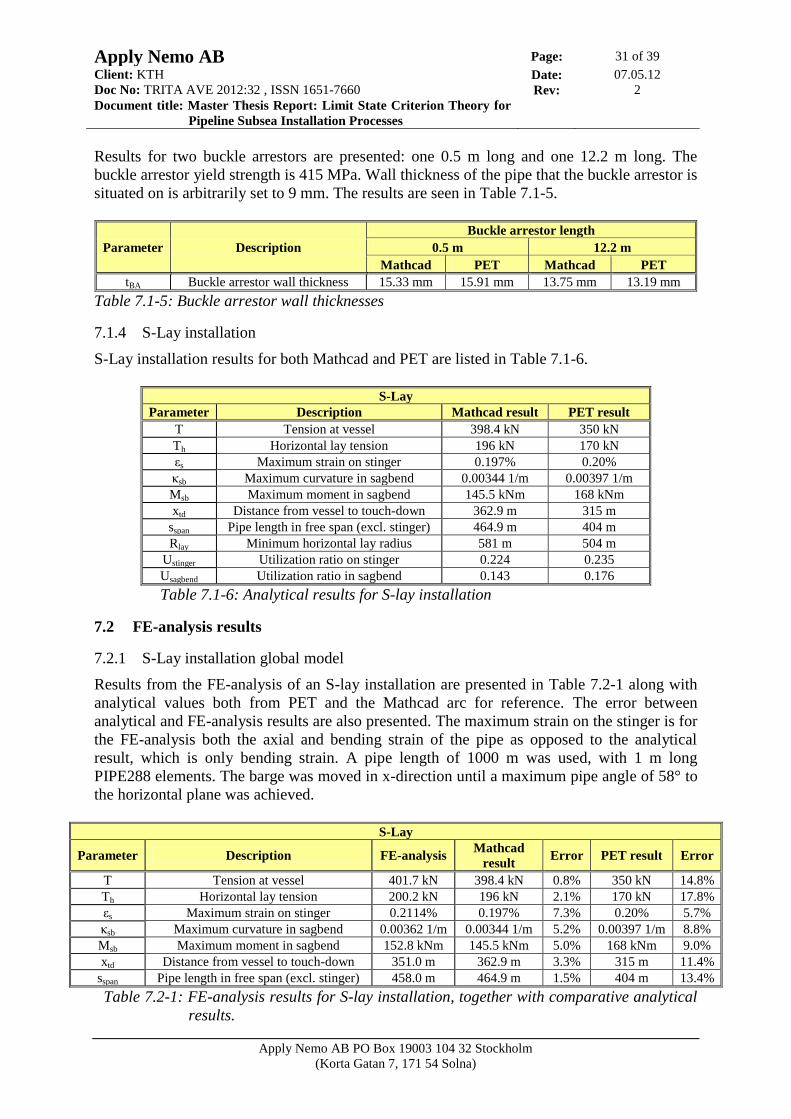
Stresses at 12 o’clock and 6 o’clock of the pipe are averaged for the pipe length, excluding the
first and last 5m to account for boundary effects. The stress distribution for a piece of the pipe
is shown in Figure 7.2-1, also illustrating the 12 o’clock and 6 o’clock locations.
Figure 7.2-1: Stress distribution of deformed pipeline submodel. The 12 o’clock and 6 o’clock
locations are marked as red lines.
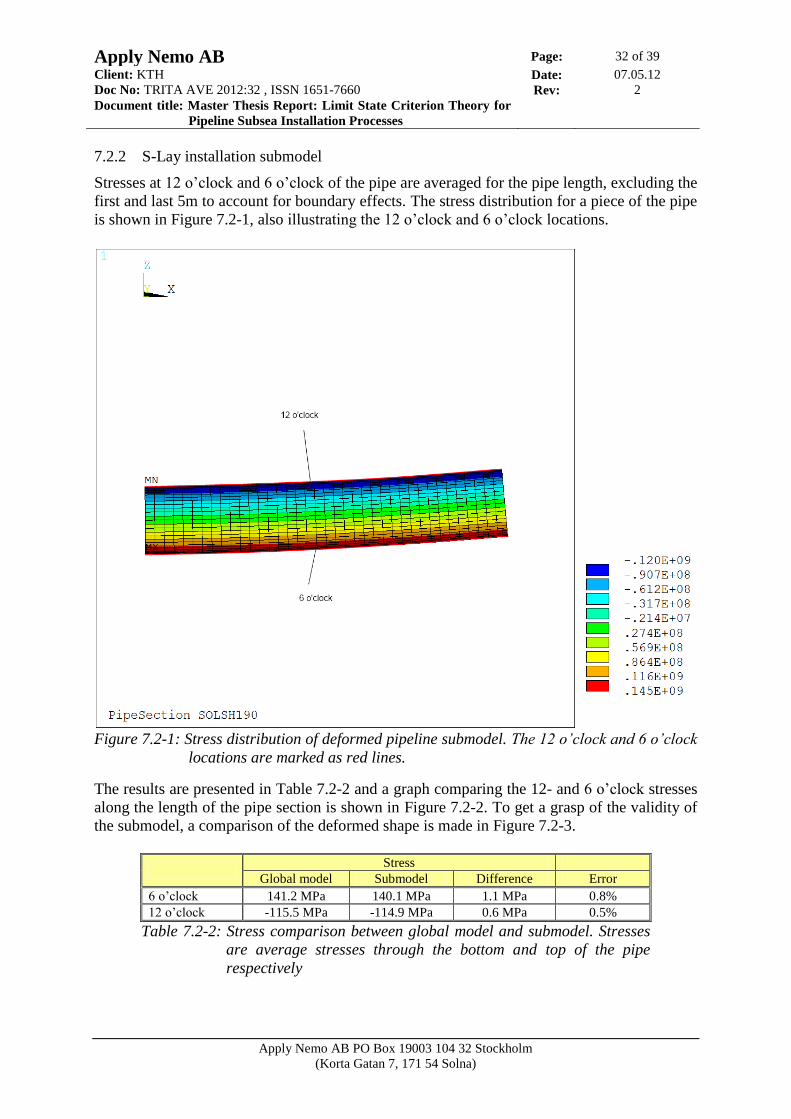
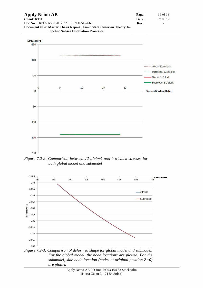
The results are presented in Table 7.2-2 and a graph comparing the 12- and 6 o’clock stresses
along the length of the pipe section is shown in Figure 7.2-2. To get a grasp of the validity of
the submodel, a comparison of the deformed shape is made in Figure 7.2-3.
Stress
Global model Submodel Difference Error
6 o’clock 141.2 MPa 140.1 MPa 1.1 MPa 0.8%
12 o’clock -115.5 MPa -114.9 MPa 0.6 MPa 0.5%
Table 7.2-2: Stress comparison between global model and submodel. Stresses
are average stresses through the bottom and top of the pipe
respectively
Apply Nemo AB Page: 33 of 39
Client: KTH Date: 07.05.12
Doc No: TRITA AVE 2012:32 , ISSN 1651-7660 Rev: 2
Document title: Master Thesis Report: Limit State Criterion Theory for
Pipeline Subsea Installation Processes
Apply Nemo AB PO Box 19003 104 32 Stockholm
(Korta Gatan 7, 171 54 Solna)
Figure 7.2-2: Comparison between 12 o’clock and 6 o’clock stresses for
both global model and submodel
Figure 7.2-3: Comparison of deformed shape for global model and submodel.
For the global model, the node locations are plotted. For the
submodel, side node location (nodes at original position Z=0)
are plotted
Apply Nemo AB Page: 34 of 39
Client: KTH Date: 07.05.12
Doc No: TRITA AVE 2012:32 , ISSN 1651-7660 Rev: 2
Document title: Master Thesis Report: Limit State Criterion Theory for
Pipeline Subsea Installation Processes
Apply Nemo AB PO Box 19003 104 32 Stockholm
(Korta Gatan 7, 171 54 Solna)
7.2.3 S-Lay minimum lay radius model
The horizontal tension Th=196 kN and the minimum lay radius Rlay=581 m from the Mathcad
results was used as input data for the minimum curvature FE-model. The greatest deviation of
the pipe from its original position was found to be 0.170 m at the pipe end, which is well
below the tolerable 1 m limit. By increasing the horizontal tension by 10%, the deviation was
found to be 0.877 m, again at the pipe end where the load was applied. If, however, the load
found in the FE-analysis was applied, the maximum deviations were 0.219 m at Th=200.2 kN
and 1.12 m at 10% increased load.
Apply Nemo AB Page: 35 of 39
Client: KTH Date: 07.05.12
Doc No: TRITA AVE 2012:32 , ISSN 1651-7660 Rev: 2
Document title: Master Thesis Report: Limit State Criterion Theory for
Pipeline Subsea Installation Processes
Apply Nemo AB PO Box 19003 104 32 Stockholm
(Korta Gatan 7, 171 54 Solna)
8 DISCUSSION
8.1 General
The discussion section is divided into six parts, one for each limit state and one for each
model. The S-Lay installation theory and FE-analysis is discussed in the same section. In
sections concerning limit states, results for both the old and new DNV standards (that is, both
PET and the Mathcad arc) are presented and discussed. Limitations to the theoretical models
are also mentioned. No explanations to changes in the DNV standard are given, as DNV
provides no change-log.
Notable differences between the FE-analyses results’ and the analytical results are discussed,
and limitations to the FE-models are mentioned.
8.2 Bursting
As seen in Table 7.1-2, results between PET and Mathcad do not differ significantly. The
difference seen is due to rounding errors in the calculations. The required thickness for
bursting is in this specific case equal to that of propagating buckling – this is however sheer
coincidence. As expected at this small water depth, the bursting limit state is dimensioning for
the pipeline’s wall thickness. As depth increases, the external pressure from the water will
counteract the internal pressure inside the pipe, giving smaller wall thickness requirements.
This can be better understood by looking at the limit state criterion in equation (5.2.1).
8.3 Collapse/Local buckling
The limit state criterion is changed in the new standards, removing a safety factor of 1.1. This
would imply that the new standard is less conservative, which can be seen in the bottom row
of Table 7.1-3. In the new standard, fabrication tolerances should however be included in the
calculation of the characteristic collapse pressure, and this affects the wall thickness. As seen
in the top row of Table 7.1-3, if a fabrication tolerance of 12.5% is included the required wall
thickness is increased. The new standard is therefore both more and less conservative than the
old one, depending on how much fabrication tolerance is included.
8.4 Propagating buckling
The differences between the two standards are not seen until buckle arrestors are considered.
As a safety factor of 1.1 is removed in the new standard, results for both infinitely long and
infinitely short arrestors differ between the two standards. If, however, this factor were to
remain, results for infinitely long arrestors are the same whilst results for short arrestors vary,
as these are dependant more on the exponential in the cross-over pressure in equation (5.4.4).
A pipe section of 12.2 m (one standard pipe length) is considered infinitely long in the
context. Inserting smaller sections is also an option, but it is far simpler and far more
economically viable to just insert a thicker 12.2 m pipe section.
Discussion can be made to the relevance of buckle arrestors in the pipeline to begin with –
their existence is based upon there being allowance for propagating buckling to occur in the
pipeline, something that should be avoided. A more common approach is to simply make the
entire pipe thicker, avoiding the problem altogether although at a higher material cost.
Apply Nemo AB Page: 36 of 39
Client: KTH Date: 07.05.12
Doc No: TRITA AVE 2012:32 , ISSN 1651-7660 Rev: 2
Document title: Master Thesis Report: Limit State Criterion Theory for
Pipeline Subsea Installation Processes
Apply Nemo AB PO Box 19003 104 32 Stockholm
(Korta Gatan 7, 171 54 Solna)
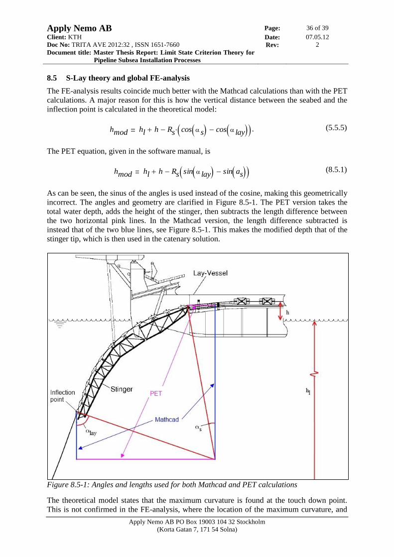
8.5 S-Lay theory and global FE-analysis
The FE-analysis results coincide much better with the Mathcad calculations than with the PET
calculations. A major reason for this is how the vertical distance between the seabed and the
inflection point is calculated in the theoretical model:
. (5.5.5)
The PET equation, given in the software manual, is
(8.5.1)
As can be seen, the sinus of the angles is used instead of the cosine, making this geometrically
incorrect. The angles and geometry are clarified in Figure 8.5-1. The PET version takes the
total water depth, adds the height of the stinger, then subtracts the length difference between
the two horizontal pink lines. In the Mathcad version, the length difference subtracted is
instead that of the two blue lines, see Figure 8.5-1. This makes the modified depth that of the
stinger tip, which is then used in the catenary solution.
Figure 8.5-1: Angles and lengths used for both Mathcad and PET calculations
The theoretical model states that the maximum curvature is found at the touch down point.
This is not confirmed in the FE-analysis, where the location of the maximum curvature, and
hmod hl h Rs cos s cos lay
hmod hl h Rs sin lay sin as
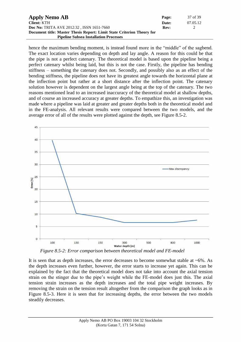
Apply Nemo AB Page: 37 of 39
Client: KTH Date: 07.05.12
Doc No: TRITA AVE 2012:32 , ISSN 1651-7660 Rev: 2
Document title: Master Thesis Report: Limit State Criterion Theory for
Pipeline Subsea Installation Processes
Apply Nemo AB PO Box 19003 104 32 Stockholm
(Korta Gatan 7, 171 54 Solna)
hence the maximum bending moment, is instead found more in the “middle” of the sagbend.
The exact location varies depending on depth and lay angle. A reason for this could be that
the pipe is not a perfect catenary. The theoretical model is based upon the pipeline being a
perfect catenary whilst being laid, but this is not the case. Firstly, the pipeline has bending
stiffness – something the catenary does not. Secondly, and possibly also as an effect of the
bending stiffness, the pipeline does not have its greatest angle towards the horizontal plane at
the inflection point but rather at a short distance after the inflection point. The catenary
solution however is dependent on the largest angle being at the top of the catenary. The two
reasons mentioned lead to an increased inaccuracy of the theoretical model at shallow depths,
and of course an increased accuracy at greater depths. To empathize this, an investigation was
made where a pipeline was laid at greater and greater depths both in the theoretical model and
in the FE-analysis. All relevant results were compared between the two models, and the
average error of all of the results were plotted against the depth, see Figure 8.5-2.
Figure 8.5-2: Error comparison between theoretical model and FE-model
It is seen that as depth increases, the error decreases to become somewhat stable at ~6%. As
the depth increases even further, however, the error starts to increase yet again. This can be
explained by the fact that the theoretical model does not take into account the axial tension
strain on the stinger due to the pipe’s weight while the FE-model does just this. The axial
tension strain increases as the depth increases and the total pipe weight increases. By
removing the strain on the tension result altogether from the comparison the graph looks as in
Figure 8.5-3. Here it is seen that for increasing depths, the error between the two models
steadily decreases.
Apply Nemo AB Page: 38 of 39
Client: KTH Date: 07.05.12
Doc No: TRITA AVE 2012:32 , ISSN 1651-7660 Rev: 2
Document title: Master Thesis Report: Limit State Criterion Theory for
Pipeline Subsea Installation Processes
Apply Nemo AB PO Box 19003 104 32 Stockholm
(Korta Gatan 7, 171 54 Solna)
Figure 8.5-3: Error comparison when excluding the strain result
8.6 S-Lay submodel
The submodel is used to investigate more thoroughly the stress distribution of the pipeline
where the maximum curvature is gotten. This is done using another type of element and a
finer mesh. The global model and the submodel coincide very well, indicating that the
PIPE288 elements used in the global model should produce satisfactory results. Should
however the global model be faulty or not reflect reality good enough, this will also be the
case in the submodel as data from the global model is used as input data for the submodel.
The submodel should as such be seen as a verification of the global model, not of the
installation process itself.
The submodel is 24 m long, meaning that in reality at least one weld would be included in the
modelled section. Weld effects are outside of this report’s scope, and are thus not taken into
account in this analysis nor in the global model analysis. It is highly likely that stress
concentrations occur in welds and this might affect the geometry of the pipe during S-Lay.
8.7 S-Lay minimum curvature model
The greatest deviations from the original position were found at the end where the horizontal
tension was applied. This is because the pipeline is held in place by the friction towards the
seabed, and the applied force is absorbed by this friction as the distance from the force’s
application point increases. The results gotten from the Mathcad arc indicates that the theory
is a bit conservative, as an increase by 10% of the horizontal tension did not move the pipe
more than the 1 m limit. When using the FE-analysis resulting horizontal tension from the
global model as input data however, an increase in 10% of the tension did make the pipe
move more than 1 m. The FE-model is less conservative in this respect.
Apply Nemo AB Page: 39 of 39
Client: KTH Date: 07.05.12
Doc No: TRITA AVE 2012:32 , ISSN 1651-7660 Rev: 2
Document title: Master Thesis Report: Limit State Criterion Theory for
Pipeline Subsea Installation Processes
Apply Nemo AB PO Box 19003 104 32 Stockholm
(Korta Gatan 7, 171 54 Solna)
9 REFERENCES
/1/ http://www.subseaworld.com/news/technip-set-ultra-deepwater-pipeline-
installation-records-02874.html, , "" , 2012-04-12
/2/ Jaeyoung Lee, P.E, , "Introduction to Offshore Pipelines and Risers" , 2008
/3/ DNV OS-F101 2010, DNV, "Submarine Pipeline Systems" , doc. no. DNV-OS-
F101, Rev. October 2010
/4/ Kyriakides, S., 978-0-08-046732-0, "Mechanics of Offshore Pipelines Volume 1:
Buckling and Collapse" , 2007
/5/ DNV OS-F101 2000, DNV, "Submarine Pipeline Systems" , doc. no. DNV-OS-
F101, 2000
/6/ Bai, Y., 0-080-4456-67, "Subsea Pipelines and Risers" , 2005