Embed Size (px)
Citation preview

December 15, 2011 Eindhoven
Internship report
Coach: Dr. R. E. Erkmen
University of Technology Sydney Department of Civil Engineering
Supervisor: Prof. Dr. M.G.D Geers
Technische Universiteit Eindhoven Department of Mechanical Engineering Division of Computational and Experimental mechanics
Application of Shell elements to buckling-analyses of thin-walled
composite laminates
B.A. Gӧttgens
MT 12.02
Internship report B.A. Gӧttgens 0727452
2
Contents
Contents .......................................................................................................................................... 2
1 Introduction .................................................................................................................................. 3
2 Validation of the numerical tool .................................................................................................. 6
2.1 One-dimensional beam buckling .......................................................................................... 6
2.2 Plate deflections .................................................................................................................... 9
2.4 One-dimensional thin-walled beam buckling ..................................................................... 17
2.5 Thin-walled beam buckling ................................................................................................ 20
3 Parametric case studies .............................................................................................................. 24
3.1 Effect of laminate layup on critical buckling load .............................................................. 24
3.2 Transition from lateral to local buckling behavior ............................................................. 26
4 Convergence studies .................................................................................................................. 28
4.1 Mesh conditions for twist-Kirchhoff shell element ............................................................ 28
4.2 Convergence studies on square plates ................................................................................ 29
5 Conclusions ................................................................................................................................ 35
Bibliography ................................................................................................................................. 36
Appendix 1 Derivation of stiffness matrices ................................................................................ 37
Internship report B.A. Gӧttgens 0727452
3
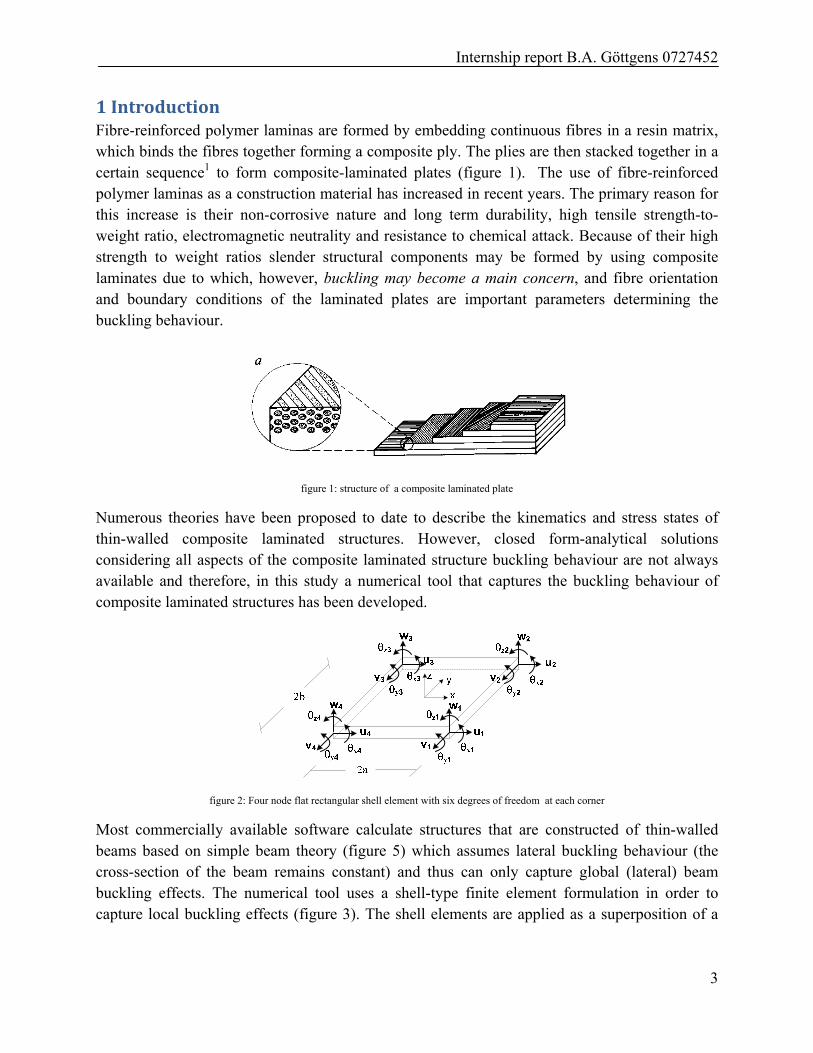
1IntroductionFibre-reinforced polymer laminas are formed by embedding continuous fibres in a resin matrix, which binds the fibres together forming a composite ply. The plies are then stacked together in a certain sequence1 to form composite-laminated plates (figure 1). The use of fibre-reinforced polymer laminas as a construction material has increased in recent years. The primary reason for this increase is their non-corrosive nature and long term durability, high tensile strength-to-weight ratio, electromagnetic neutrality and resistance to chemical attack. Because of their high strength to weight ratios slender structural components may be formed by using composite laminates due to which, however, buckling may become a main concern, and fibre orientation and boundary conditions of the laminated plates are important parameters determining the buckling behaviour.
figure 1: structure of a composite laminated plate
Numerous theories have been proposed to date to describe the kinematics and stress states of thin-walled composite laminated structures. However, closed form-analytical solutions considering all aspects of the composite laminated structure buckling behaviour are not always available and therefore, in this study a numerical tool that captures the buckling behaviour of composite laminated structures has been developed.
figure 2: Four node flat rectangular shell element with six degrees of freedom at each corner
Most commercially available software calculate structures that are constructed of thin-walled beams based on simple beam theory (figure 5) which assumes lateral buckling behaviour (the cross-section of the beam remains constant) and thus can only capture global (lateral) beam buckling effects. The numerical tool uses a shell-type finite element formulation in order to capture local buckling effects (figure 3). The shell elements are applied as a superposition of a
Internship report B.A. Gӧttgens 0727452
4
four node rectangular plate with a four node rectangular membrane with six degrees of freedom per node (figure 2).
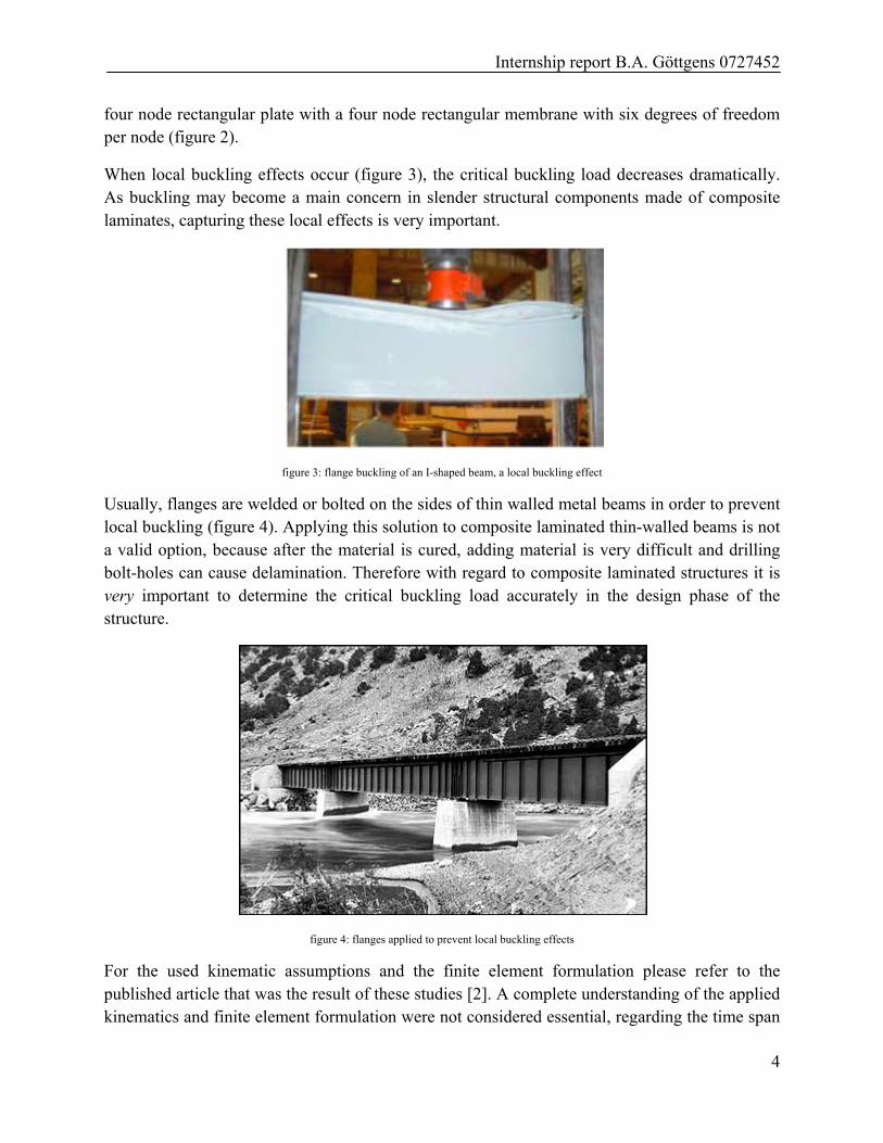
When local buckling effects occur (figure 3), the critical buckling load decreases dramatically. As buckling may become a main concern in slender structural components made of composite laminates, capturing these local effects is very important.
figure 3: flange buckling of an I-shaped beam, a local buckling effect
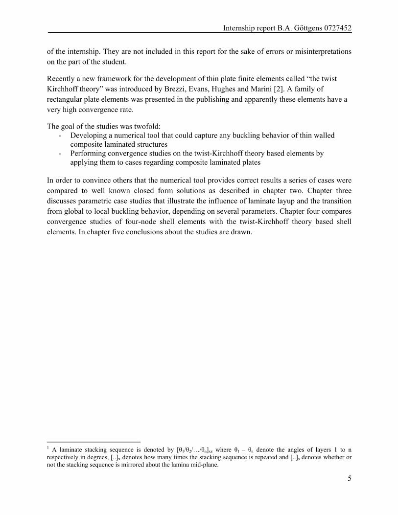
Usually, flanges are welded or bolted on the sides of thin walled metal beams in order to prevent local buckling (figure 4). Applying this solution to composite laminated thin-walled beams is not a valid option, because after the material is cured, adding material is very difficult and drilling bolt-holes can cause delamination. Therefore with regard to composite laminated structures it is very important to determine the critical buckling load accurately in the design phase of the structure.
figure 4: flanges applied to prevent local buckling effects
For the used kinematic assumptions and the finite element formulation please refer to the published article that was the result of these studies [2]. A complete understanding of the applied kinematics and finite element formulation were not considered essential, regarding the time span
Internship report B.A. Gӧttgens 0727452
5
of the internship. They are not included in this report for the sake of errors or misinterpretations on the part of the student.
Recently a new framework for the development of thin plate finite elements called “the twist Kirchhoff theory” was introduced by Brezzi, Evans, Hughes and Marini [2]. A family of rectangular plate elements was presented in the publishing and apparently these elements have a very high convergence rate.
The goal of the studies was twofold: - Developing a numerical tool that could capture any buckling behavior of thin walled
composite laminated structures - Performing convergence studies on the twist-Kirchhoff theory based elements by
applying them to cases regarding composite laminated plates In order to convince others that the numerical tool provides correct results a series of cases were compared to well known closed form solutions as described in chapter two. Chapter three discusses parametric case studies that illustrate the influence of laminate layup and the transition from global to local buckling behavior, depending on several parameters. Chapter four compares convergence studies of four-node shell elements with the twist-Kirchhoff theory based shell elements. In chapter five conclusions about the studies are drawn.
1
1 A laminate stacking sequence is denoted by [θ1/θ2/…/θn]xs where θ1 – θn denote the angles of layers 1 to n respectively in degrees, [..]x denotes how many times the stacking sequence is repeated and [..]s denotes whether or not the stacking sequence is mirrored about the lamina mid-plane.
Internship report B.A. Gӧttgens 0727452
6
2ValidationofthenumericaltoolPrior to convergence and parametric case studies, the tool was validated by comparing several cases to well known closed form solutions.
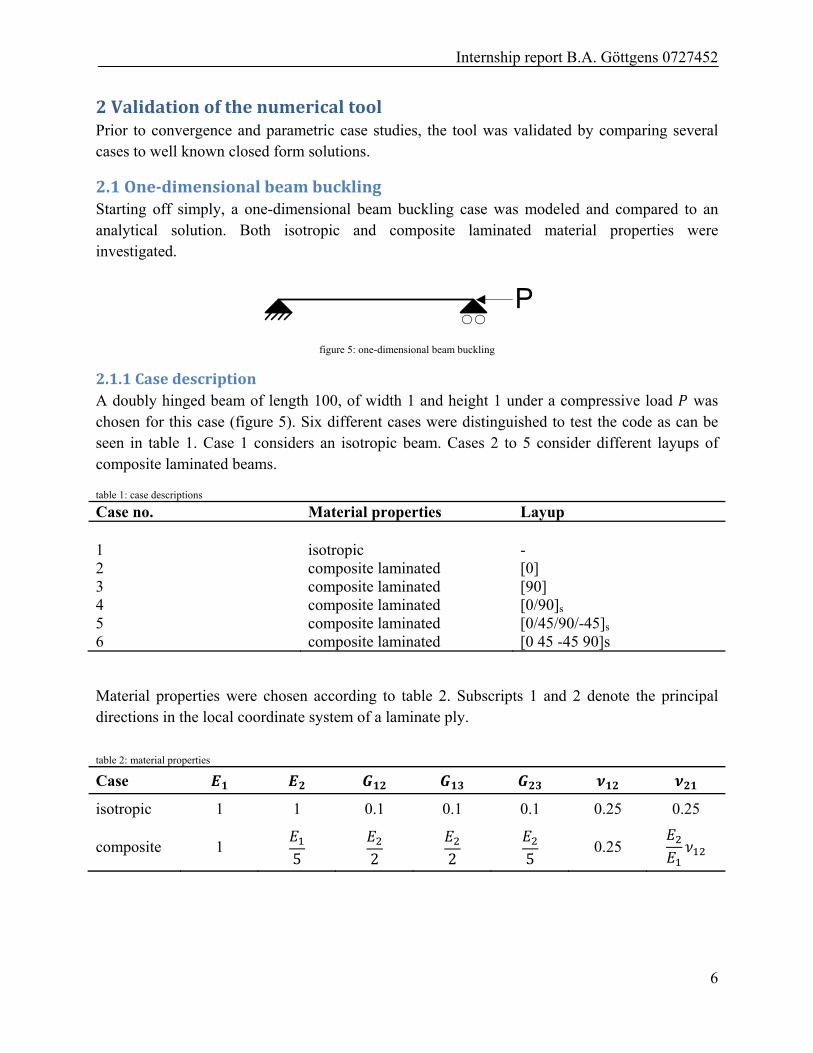
2.1One‐dimensionalbeambucklingStarting off simply, a one-dimensional beam buckling case was modeled and compared to an analytical solution. Both isotropic and composite laminated material properties were investigated.
figure 5: one-dimensional beam buckling
2.1.1CasedescriptionA doubly hinged beam of length 100, of width 1 and height 1 under a compressive load was chosen for this case (figure 5). Six different cases were distinguished to test the code as can be seen in table 1. Case 1 considers an isotropic beam. Cases 2 to 5 consider different layups of composite laminated beams.
table 1: case descriptions
Case no. Material properties Layup 1 isotropic - 2 composite laminated [0] 3 composite laminated [90] 4 composite laminated [0/90]s
5 composite laminated [0/45/90/-45]s
6 composite laminated [0 45 -45 90]s
Material properties were chosen according to table 2. Subscripts 1 and 2 denote the principal directions in the local coordinate system of a laminate ply.
table 2: material properties
Case
isotropic 1 1 0.1 0.1 0.1 0.25 0.25
composite 1 5
2
2
5
0.25
Internship report B.A. Gӧttgens 0727452
7
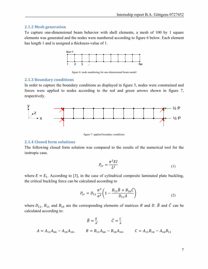
2.1.2MeshgenerationTo capture one-dimensional beam behavior with shell elements, a mesh of 100 by 1 square elements was generated and the nodes were numbered according to figure 6 below. Each element has length 1 and is assigned a thickness-value of 1.
figure 6: node numbering for one-dimensional beam model
2.1.3BoundaryconditionsIn order to capture the boundary conditions as displayed in figure 5, nodes were constrained and forces were applied to nodes according to the red and green arrows shown in figure 7, respectively.
½ P
½ Px
y
z
figure 7: applied boundary conditions
2.1.4ClosedformsolutionsThe following closed form solution was compared to the results of the numerical tool for the isotropic case.
(1)
where . According to [3], in the case of cylindrical composite laminated plate buckling, the critical buckling force can be calculated according to
1
(2)
where , and are the corresponding elements of matrices and . and can be calculated according to:
,
, ,
Internship report B.A. Gӧttgens 0727452
8
where and are elements of matrices and . For the determination of extensional
stiffness matrix , coupling stiffness matrix and bending stiffness matrix please refer to appendix 1.
2.1.5ResultsAll six cases were run with the numerical tool. The resulting values for the critical applied load were compared to the closed form solutions and are displayed in table 3 below.
table 3: resulting critical applied loads
Case no Numerical tool (3) (4) 1 8.257E-05 8.22E-05
(0.0390) 8.773E-05
(0.06251)
2 8.257E-05 - 8.773E-05 (0.06251)
3 1.645E-05 - 1.666E-05 (0.01257)
4 7.427E-05 - 7.496E-06 (0.00926)
5 5.835E-05 - 6.100E-05 (0.04553)
6 5.865E-05 - 6..275E-05 (0.06996)
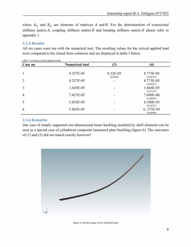
2.1.6RemarksOur case of simply supported one-dimensional beam buckling modeled by shell elements can be seen as a special case of cylindrical composite laminated plate buckling (figure 8). The outcomes of (1) and (2) did not match exactly however!
figure 8: buckled shape of the modeled beam
Internship report B.A. Gӧttgens 0727452
9
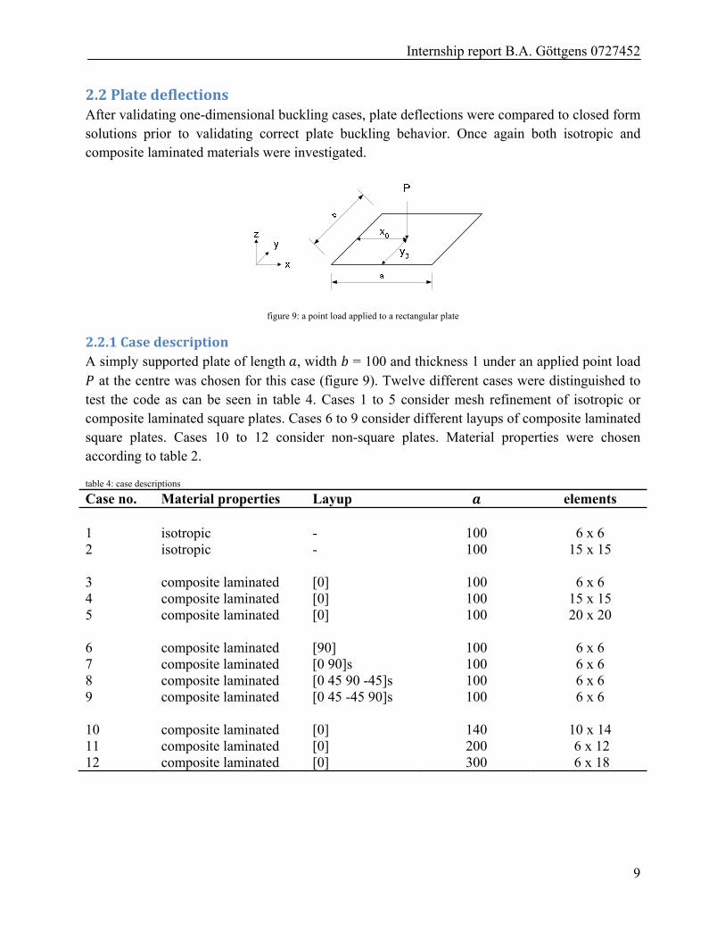
2.2PlatedeflectionsAfter validating one-dimensional buckling cases, plate deflections were compared to closed form solutions prior to validating correct plate buckling behavior. Once again both isotropic and composite laminated materials were investigated.
figure 9: a point load applied to a rectangular plate
2.2.1CasedescriptionA simply supported plate of length , width = 100 and thickness 1 under an applied point load
at the centre was chosen for this case (figure 9). Twelve different cases were distinguished to test the code as can be seen in table 4. Cases 1 to 5 consider mesh refinement of isotropic or composite laminated square plates. Cases 6 to 9 consider different layups of composite laminated square plates. Cases 10 to 12 consider non-square plates. Material properties were chosen according to table 2.
table 4: case descriptions
Case no. Material properties Layup elements 1 isotropic - 100 6 x 6 2 isotropic - 100 15 x 15 3 composite laminated [0] 100 6 x 6 4 composite laminated [0] 100 15 x 15 5 composite laminated [0] 100 20 x 20 6 composite laminated [90] 100 6 x 6 7 composite laminated [0 90]s 100 6 x 6 8 composite laminated [0 45 90 -45]s 100 6 x 6 9 composite laminated [0 45 -45 90]s 100 6 x 6 10 composite laminated [0] 140 10 x 14 11 composite laminated [0] 200 6 x 12 12 composite laminated [0] 300 6 x 18
Internship report B.A. Gӧttgens 0727452
10
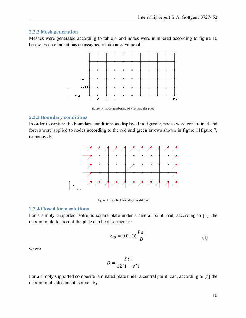
2.2.2MeshgenerationMeshes were generated according to table 4 and nodes were numbered according to figure 10 below. Each element has an assigned a thickness-value of 1.
figure 10: node numbering of a rectangular plate
2.2.3BoundaryconditionsIn order to capture the boundary conditions as displayed in figure 9, nodes were constrained and forces were applied to nodes according to the red and green arrows shown in figure 11figure 7, respectively.
figure 11: applied boundary conditions
2.2.4ClosedformsolutionsFor a simply supported isotropic square plate under a central point load, according to [4], the maximum deflection of the plate can be described as:
0.0116
(3)
where
12 1
For a simply supported composite laminated plate under a central point load, according to [5] the maximum displacement is given by
Internship report B.A. Gӧttgens 0727452
11
sin sin
(4)
where
4
sin sin
2
Where is the ratio of over (the aspect ratio). , and represent elements , and combination of elements 2 from matrix , respectively. Scalars and are defined as:
,
Where and are defined as the modes of buckling in x- and y-directions, respectively.
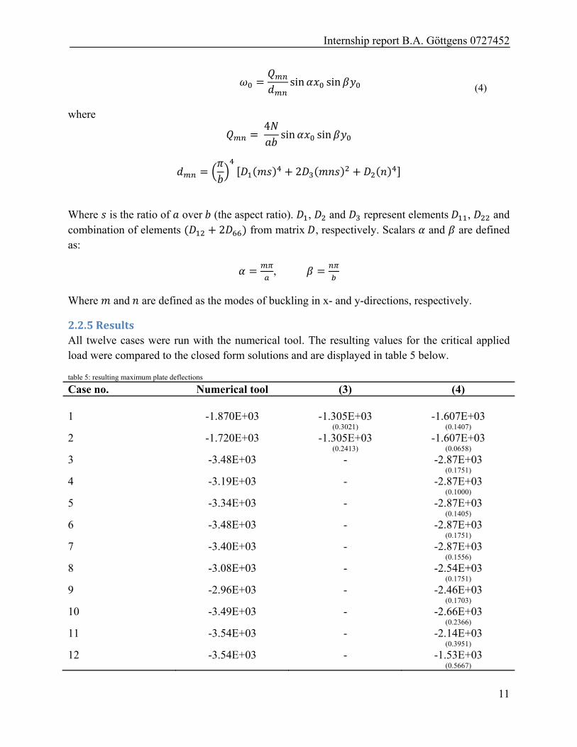
2.2.5ResultsAll twelve cases were run with the numerical tool. The resulting values for the critical applied load were compared to the closed form solutions and are displayed in table 5 below.
table 5: resulting maximum plate deflections
Case no. Numerical tool (3) (4) 1 -1.870E+03 -1.305E+03
(0.3021) -1.607E+03
(0.1407)
2 -1.720E+03 -1.305E+03 (0.2413)
-1.607E+03 (0.0658)
3 -3.48E+03 - -2.87E+03 (0.1751)
4 -3.19E+03 - -2.87E+03 (0.1000)
5 -3.34E+03 - -2.87E+03 (0.1405)
6 -3.48E+03 - -2.87E+03 (0.1751)
7 -3.40E+03 - -2.87E+03 (0.1556)
8 -3.08E+03 - -2.54E+03 (0.1751)
9 -2.96E+03 - -2.46E+03 (0.1703)
10 -3.49E+03 - -2.66E+03 (0.2366)
11 -3.54E+03 - -2.14E+03 (0.3951)
12 -3.54E+03 - -1.53E+03 (0.5667)
Internship report B.A. Gӧttgens 0727452
12
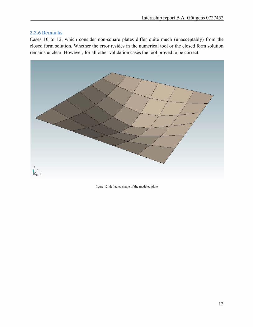
2.2.6RemarksCases 10 to 12, which consider non-square plates differ quite much (unacceptably) from the closed form solution. Whether the error resides in the numerical tool or the closed form solution remains unclear. However, for all other validation cases the tool proved to be correct.
figure 12: deflected shape of the modeled plate
Internship report B.A. Gӧttgens 0727452
13
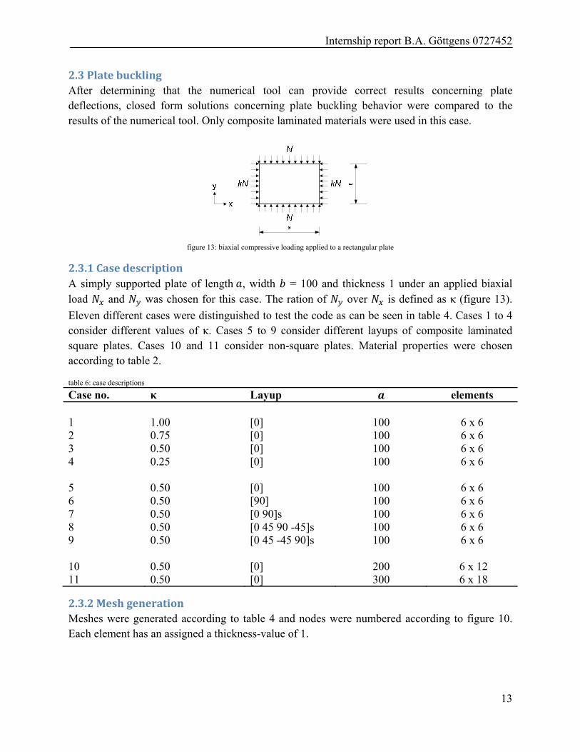
2.3PlatebucklingAfter determining that the numerical tool can provide correct results concerning plate deflections, closed form solutions concerning plate buckling behavior were compared to the results of the numerical tool. Only composite laminated materials were used in this case.
figure 13: biaxial compressive loading applied to a rectangular plate
2.3.1CasedescriptionA simply supported plate of length , width = 100 and thickness 1 under an applied biaxial load and was chosen for this case. The ration of over is defined as κ (figure 13).
Eleven different cases were distinguished to test the code as can be seen in table 4. Cases 1 to 4 consider different values of κ. Cases 5 to 9 consider different layups of composite laminated square plates. Cases 10 and 11 consider non-square plates. Material properties were chosen according to table 2.
table 6: case descriptions
Case no. κ Layup elements 1 1.00 [0] 100 6 x 6 2 0.75 [0] 100 6 x 6 3 0.50 [0] 100 6 x 6 4 0.25 [0] 100 6 x 6 5 0.50 [0] 100 6 x 6 6 0.50 [90] 100 6 x 6 7 0.50 [0 90]s 100 6 x 6 8 0.50 [0 45 90 -45]s 100 6 x 6 9 0.50 [0 45 -45 90]s 100 6 x 6 10 0.50 [0] 200 6 x 12 11 0.50 [0] 300 6 x 18
2.3.2MeshgenerationMeshes were generated according to table 4 and nodes were numbered according to figure 10. Each element has an assigned a thickness-value of 1.
Internship report B.A. Gӧttgens 0727452
14
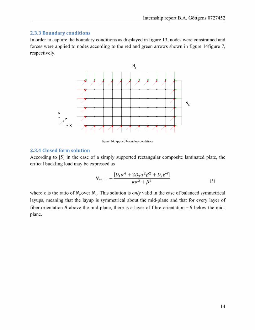
2.3.3BoundaryconditionsIn order to capture the boundary conditions as displayed in figure 13, nodes were constrained and forces were applied to nodes according to the red and green arrows shown in figure 14figure 7, respectively.
figure 14: applied boundary conditions
2.3.4ClosedformsolutionAccording to [5] in the case of a simply supported rectangular composite laminated plate, the critical buckling load may be expressed as
2
(5)
where κ is the ratio of over . This solution is only valid in the case of balanced symmetrical
layups, meaning that the layup is symmetrical about the mid-plane and that for every layer of
fiber-orientation above the mid-plane, there is a layer of fibre-orientation – below the mid-plane.
Internship report B.A. Gӧttgens 0727452
15
2.3.5ResultsAll eleven cases were run with the numerical tool. The resulting values for the critical applied load were compared to the closed form solutions and are displayed in table 7table 5 below.
table 7: resulting critical buckling loads
Case no. Numerical tool (5) 1 7.6156E-03 7.0586E-03
(0.07313)
2 6.5424E-03 6.0503E-03 (0.07523)
3 5.1025E-03 4.7058E-03 (0.07776)
4 3.0722E-03 2.8235E-03 (0.08097)
5 5.1025E-03 4.7058E-03 (0.07776)
6 5.0433E-03 4.7058E-03 (0.06694)
7 5.1031E-03 4.7058E-03 (0.04083)
8 5.5437E-03 5.3174E-03 (0.05375)
9 5.8133E-03 5.5009E-03 (0.07313)
10 7.4307E-03 4.2060E-03 (0.43396)
11 7.4307E-03 4.1719E-03 (0.52629)
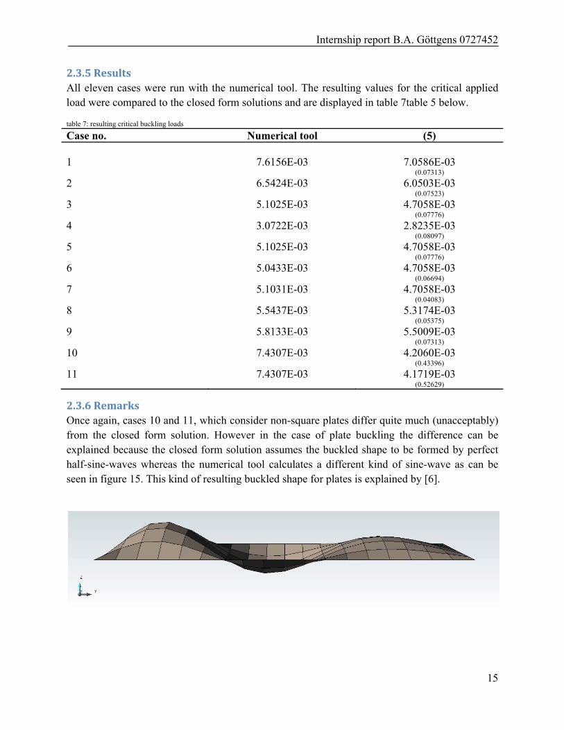
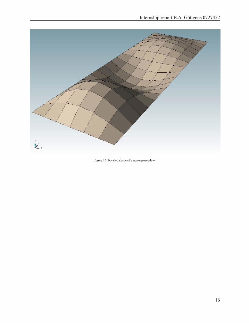
2.3.6RemarksOnce again, cases 10 and 11, which consider non-square plates differ quite much (unacceptably) from the closed form solution. However in the case of plate buckling the difference can be explained because the closed form solution assumes the buckled shape to be formed by perfect half-sine-waves whereas the numerical tool calculates a different kind of sine-wave as can be seen in figure 15. This kind of resulting buckled shape for plates is explained by [6].
Internship report B.A. Gӧttgens 0727452
16
figure 15: buckled shape of a non-square plate
Internship report B.A. Gӧttgens 0727452
17
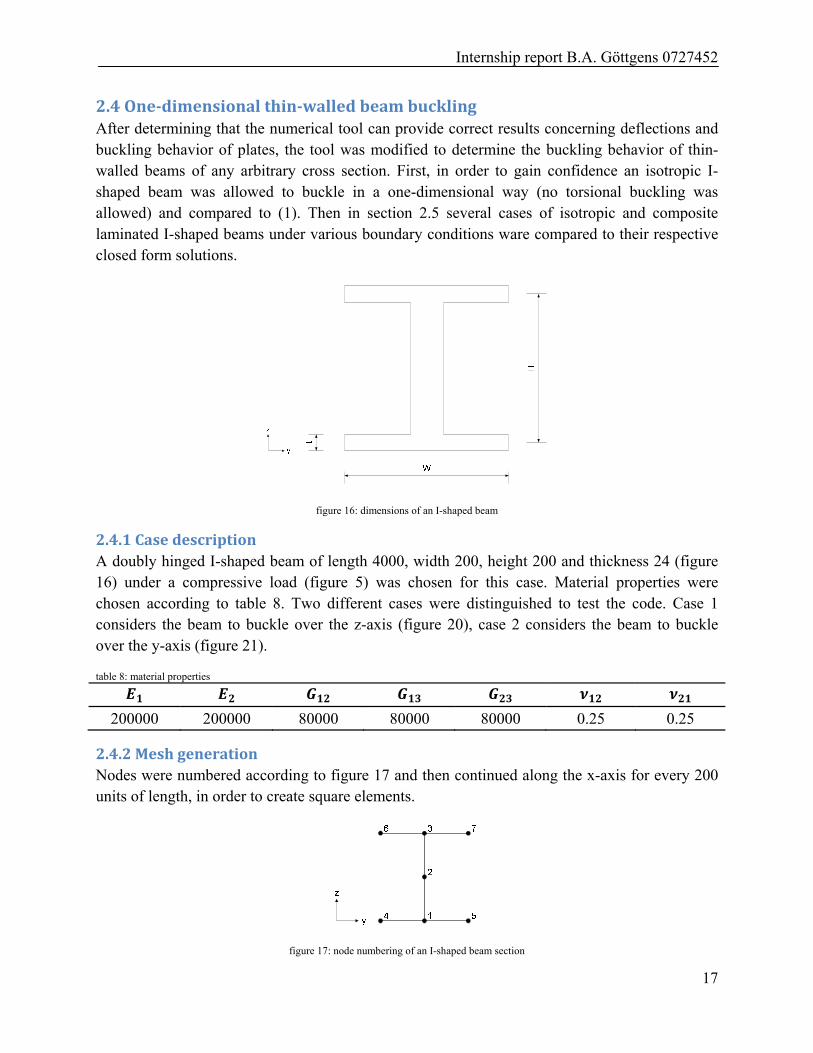
2.4One‐dimensionalthin‐walledbeambucklingAfter determining that the numerical tool can provide correct results concerning deflections and buckling behavior of plates, the tool was modified to determine the buckling behavior of thin-walled beams of any arbitrary cross section. First, in order to gain confidence an isotropic I-shaped beam was allowed to buckle in a one-dimensional way (no torsional buckling was allowed) and compared to (1). Then in section 2.5 several cases of isotropic and composite laminated I-shaped beams under various boundary conditions ware compared to their respective closed form solutions.
figure 16: dimensions of an I-shaped beam
2.4.1CasedescriptionA doubly hinged I-shaped beam of length 4000, width 200, height 200 and thickness 24 (figure 16) under a compressive load (figure 5) was chosen for this case. Material properties were chosen according to table 8. Two different cases were distinguished to test the code. Case 1 considers the beam to buckle over the z-axis (figure 20), case 2 considers the beam to buckle over the y-axis (figure 21).
table 8: material properties
200000 200000 80000 80000 80000 0.25 0.25
2.4.2MeshgenerationNodes were numbered according to figure 17 and then continued along the x-axis for every 200 units of length, in order to create square elements.
figure 17: node numbering of an I-shaped beam section
Internship report B.A. Gӧttgens 0727452
18
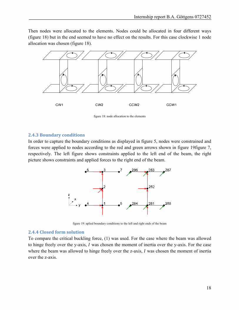
Then nodes were allocated to the elements. Nodes could be allocated in four different ways (figure 18) but in the end seemed to have no effect on the results. For this case clockwise 1 node allocation was chosen (figure 18).
figure 18: node allocation to the elements
2.4.3BoundaryconditionsIn order to capture the boundary conditions as displayed in figure 5, nodes were constrained and forces were applied to nodes according to the red and green arrows shown in figure 19figure 7, respectively. The left figure shows constraints applied to the left end of the beam, the right picture shows constraints and applied forces to the right end of the beam.
figure 19: aplied boundary conditions to the left and right ends of the beam
2.4.4ClosedformsolutionTo compare the critical buckling force, (1) was used. For the case where the beam was allowed to hinge freely over the y-axis, was chosen the moment of inertia over the y-axis. For the case where the beam was allowed to hinge freely over the z-axis, was chosen the moment of inertia over the z-axis.

Internship report B.A. Gӧttgens 0727452
19
2.4.5ResultsBoth cases were run with the numerical tool. The resulting values for the critical applied load were compared to the closed form solutions and are displayed in table 9 below.
table 9: resulting critical buckling loads
Case Numerical tool (1) 1) 4.021E+06 3.973E+06
(0.0120)
2) 1.327E+07 1.325E+07 (0.0020)
figure 20: buckled shape of the I-beam buckled over the z-axis (case 1)
figure 21: buckled shape of the I-beam buckled over the y-axis (case 2)
2.4.6RemarksTwo ways of node numbering different from figure 17 were also applied and in these cases the results were affected by the node allocations according to figure 18. So depending on the way nodes are numbered the numerical tool can become mesh-dependant.
Internship report B.A. Gӧttgens 0727452
20
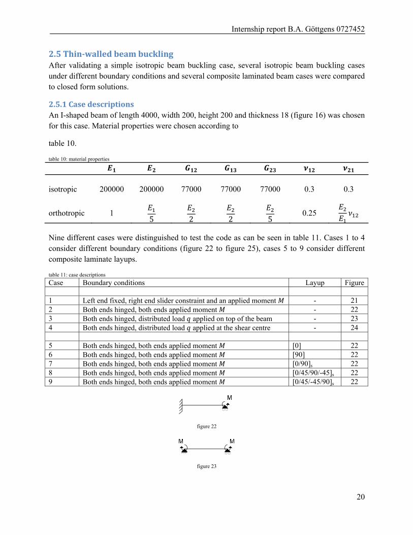
2.5Thin‐walledbeambucklingAfter validating a simple isotropic beam buckling case, several isotropic beam buckling cases under different boundary conditions and several composite laminated beam cases were compared to closed form solutions.
2.5.1CasedescriptionsAn I-shaped beam of length 4000, width 200, height 200 and thickness 18 (figure 16) was chosen for this case. Material properties were chosen according to
table 10.
table 10: material properties
isotropic 200000 200000 77000 77000 77000 0.3 0.3
orthotropic 1 5
2
2
5
0.25
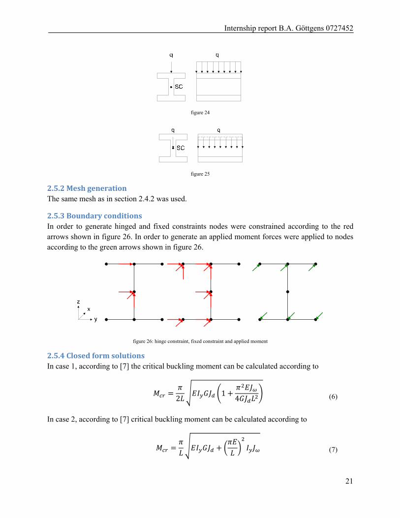
Nine different cases were distinguished to test the code as can be seen in table 11. Cases 1 to 4 consider different boundary conditions (figure 22 to figure 25), cases 5 to 9 consider different composite laminate layups.
table 11: case descriptions
Case Boundary conditions Layup Figure 1 Left end fixed, right end slider constraint and an applied moment - 21 2 Both ends hinged, both ends applied moment - 22 3 Both ends hinged, distributed load applied on top of the beam - 23 4 Both ends hinged, distributed load applied at the shear centre - 24 5 Both ends hinged, both ends applied moment [0] 22 6 Both ends hinged, both ends applied moment [90] 22 7 Both ends hinged, both ends applied moment [0/90]s 22 8 Both ends hinged, both ends applied moment [0/45/90/-45]s 22 9 Both ends hinged, both ends applied moment [0/45/-45/90]s 22
figure 22
figure 23
Internship report B.A. Gӧttgens 0727452
21
figure 24
figure 25
2.5.2MeshgenerationThe same mesh as in section 2.4.2 was used.
2.5.3BoundaryconditionsIn order to generate hinged and fixed constraints nodes were constrained according to the red arrows shown in figure 26. In order to generate an applied moment forces were applied to nodes according to the green arrows shown in figure 26.
figure 26: hinge constraint, fixed constraint and applied moment
2.5.4ClosedformsolutionsIn case 1, according to [7] the critical buckling moment can be calculated according to
21
4
(6)
In case 2, according to [7] critical buckling moment can be calculated according to
(7)
Internship report B.A. Gӧttgens 0727452
22
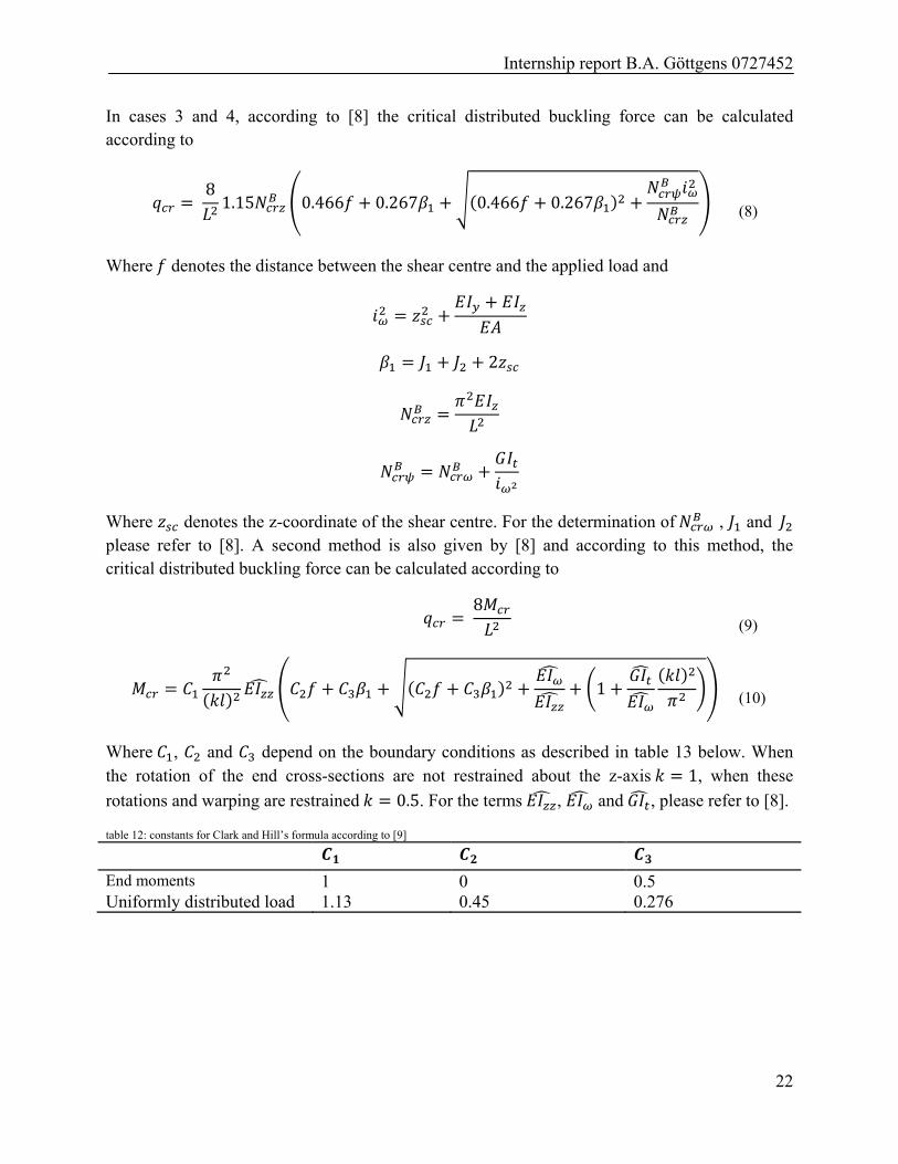
In cases 3 and 4, according to [8] the critical distributed buckling force can be calculated according to
81.15 0.466 0.267 0.466 0.267
(8)
Where denotes the distance between the shear centre and the applied load and
2
Where denotes the z-coordinate of the shear centre. For the determination of , and please refer to [8]. A second method is also given by [8] and according to this method, the critical distributed buckling force can be calculated according to
8
(9)
1
(10)
Where , and depend on the boundary conditions as described in table 13 below. When the rotation of the end cross-sections are not restrained about the z-axis 1, when these
rotations and warping are restrained 0.5. For the terms , and , please refer to [8].
table 12: constants for Clark and Hill’s formula according to [9]
End moments 1 0 0.5 Uniformly distributed load 1.13 0.45 0.276
Internship report B.A. Gӧttgens 0727452
23
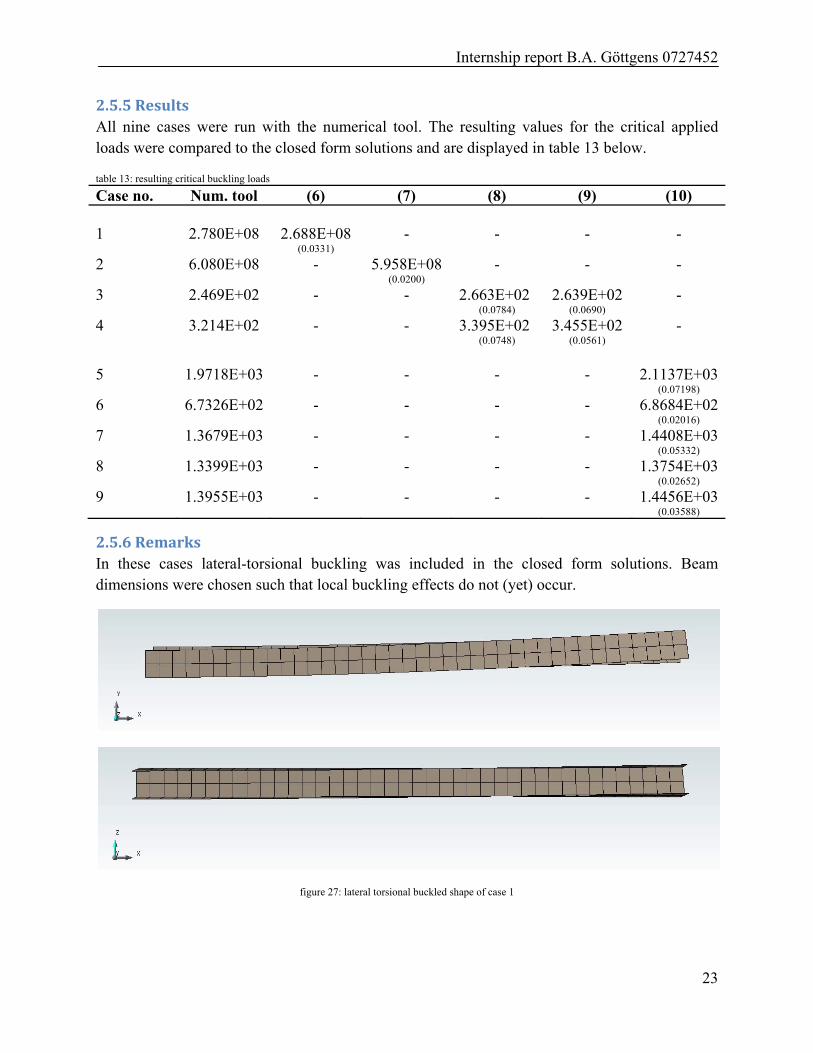
2.5.5ResultsAll nine cases were run with the numerical tool. The resulting values for the critical applied loads were compared to the closed form solutions and are displayed in table 13 below.
table 13: resulting critical buckling loads
Case no. Num. tool (6) (7) (8) (9) (10) 1 2.780E+08 2.688E+08
(0.0331) - - - -
2 6.080E+08 - 5.958E+08 (0.0200)
- - -
3 2.469E+02 - - 2.663E+02 (0.0784)
2.639E+02 (0.0690)
-
4 3.214E+02 - - 3.395E+02 (0.0748)
3.455E+02 (0.0561)
-
5 1.9718E+03 - - - - 2.1137E+03
(0.07198)
6 6.7326E+02 - - - - 6.8684E+02(0.02016)
7 1.3679E+03 - - - - 1.4408E+03(0.05332)
8 1.3399E+03 - - - - 1.3754E+03(0.02652)
9 1.3955E+03 - - - - 1.4456E+03(0.03588)
2.5.6RemarksIn these cases lateral-torsional buckling was included in the closed form solutions. Beam dimensions were chosen such that local buckling effects do not (yet) occur.
figure 27: lateral torsional buckled shape of case 1
Internship report B.A. Gӧttgens 0727452
24
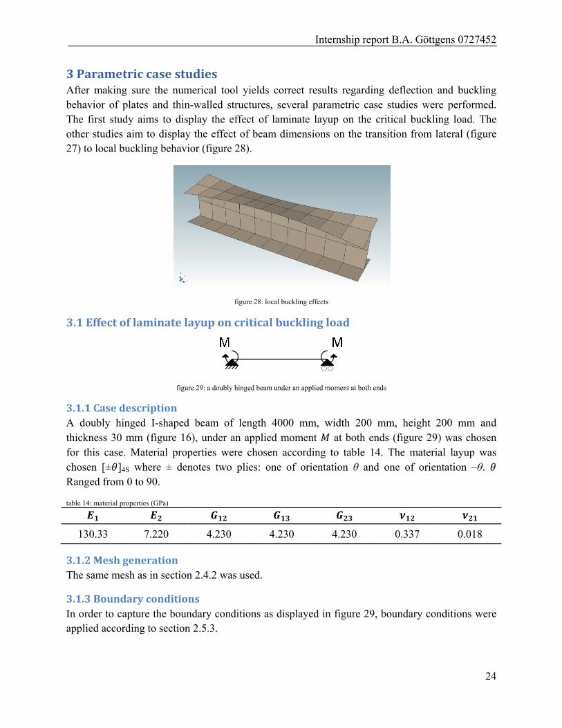
3ParametriccasestudiesAfter making sure the numerical tool yields correct results regarding deflection and buckling behavior of plates and thin-walled structures, several parametric case studies were performed. The first study aims to display the effect of laminate layup on the critical buckling load. The other studies aim to display the effect of beam dimensions on the transition from lateral (figure 27) to local buckling behavior (figure 28).
figure 28: local buckling effects
3.1Effectoflaminatelayuponcriticalbucklingload
figure 29: a doubly hinged beam under an applied moment at both ends
3.1.1CasedescriptionA doubly hinged I-shaped beam of length 4000 mm, width 200 mm, height 200 mm and thickness 30 mm (figure 16), under an applied moment at both ends (figure 29) was chosen for this case. Material properties were chosen according to table 14. The material layup was chosen [± ]4S where ± denotes two plies: one of orientation θ and one of orientation –θ. Ranged from 0 to 90.
table 14: material properties (GPa)
130.33 7.220 4.230 4.230 4.230 0.337 0.018
3.1.2MeshgenerationThe same mesh as in section 2.4.2 was used.
3.1.3BoundaryconditionsIn order to capture the boundary conditions as displayed in figure 29, boundary conditions were applied according to section 2.5.3.
Internship report B.A. Gӧttgens 0727452
25
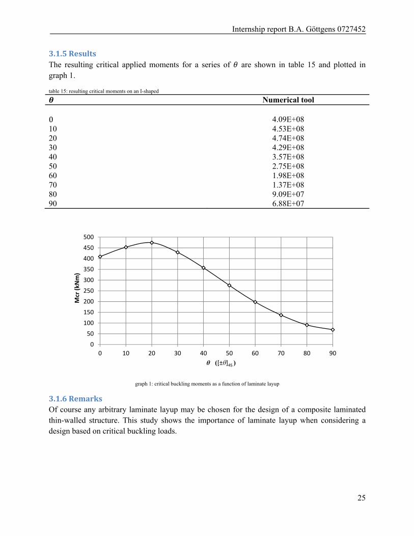
3.1.5ResultsThe resulting critical applied moments for a series of are shown in table 15 and plotted in graph 1.
table 15: resulting critical moments on an I-shaped
Numerical tool 0 4.09E+08 10 4.53E+08 20 4.74E+08 30 4.29E+08 40 3.57E+08 50 2.75E+08 60 1.98E+08 70 1.37E+08 80 9.09E+07 90 6.88E+07
graph 1: critical buckling moments as a function of laminate layup
3.1.6RemarksOf course any arbitrary laminate layup may be chosen for the design of a composite laminated thin-walled structure. This study shows the importance of laminate layup when considering a design based on critical buckling loads.
0
50
100
150
200
250
300
350
400
450
500
0 10 20 30 40 50 60 70 80 90
Mcr (kN
m)
θ ([±θ]4S )
Internship report B.A. Gӧttgens 0727452
26
3.2Transitionfromlateraltolocalbucklingbehavior
3.2.1CasedescriptionA doubly hinged I-shaped beam of width 200 mm, height 200 mm and thickness 30 mm (figure 16), under an applied moment at both ends (figure 29) was chosen for this case. Material properties were chosen according to table 14. The material layup was chosen [0]16. The beam length ranged from 1000 mm to 5000 mm.
3.2.2MeshgenerationThe same mesh as in section 2.4.2 was used.
3.2.3BoundaryconditionsIn order to capture the boundary conditions as displayed in figure 29, boundary conditions were applied according to section 2.5.3.
3.2.4ClosedformsolutionIn order to determine when local buckling effects start to dominate the buckling behavior, the results of the numerical tool were compared to (10), which assumes lateral beam buckling behavior.
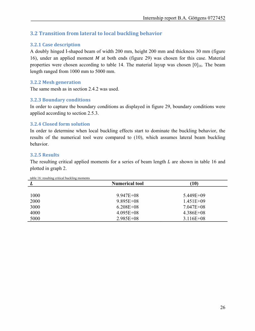
3.2.5ResultsThe resulting critical applied moments for a series of beam length are shown in table 16 and plotted in graph 2.
table 16: resulting critical buckling moments
Numerical tool (10) 1000 9.947E+08 5.449E+09 2000 9.895E+08 1.451E+09 3000 6.208E+08 7.047E+08 4000 4.095E+08 4.386E+08 5000 2.985E+08 3.116E+08
Internship report B.A. Gӧttgens 0727452
27
graph 2: critical buckling moment as a function of beam length
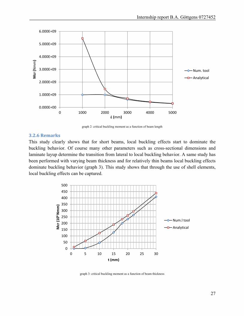
3.2.6RemarksThis study clearly shows that for short beams, local buckling effects start to dominate the buckling behavior. Of course many other parameters such as cross-sectional dimensions and laminate layup determine the transition from lateral to local buckling behavior. A same study has been performed with varying beam thickness and for relatively thin beams local buckling effects dominate buckling behavior (graph 3). This study shows that through the use of shell elements, local buckling effects can be captured.
graph 3: critical buckling moment as a function of beam thickness
0.000E+00
1.000E+09
2.000E+09
3.000E+09
4.000E+09
5.000E+09
6.000E+09
0 1000 2000 3000 4000 5000
Mcr (Nmm)
L (mm)
Num. tool
Analytical
0
50
100
150
200
250
300
350
400
450
500
0 5 10 15 20 25 30
Mcr (106 Nmm)
t (mm)
Num.l tool
Analytical
Internship report B.A. Gӧttgens 0727452
28
4ConvergencestudiesThe parametric case studies and validation were performed with a shell element named shell element 2. Two other types of shell elements were incorporated into the code, named shell element 1 and shell element 3. Shell element 1 is the simplest shell element, but quite prone to locking. Shell element 2 uses selective reduced integration to prevent locking. Shell element 3 was based on the twist-Kirchhoff theory according to [2] and supposedly has a superior convergence rate. However, according to [2] in order for the shell element to perform optimally the mesh has to meet certain conditions (as explained in section 4.1). Several convergence studies were performed in order to compare these three elements.
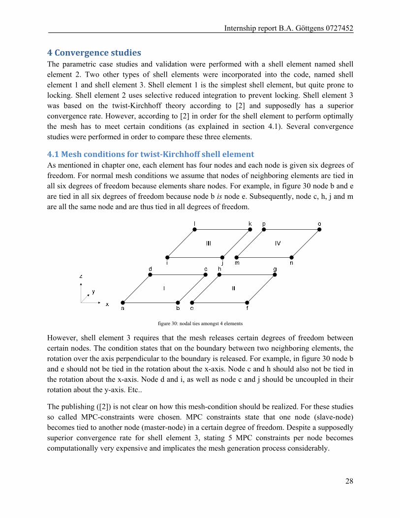
4.1Meshconditionsfortwist‐KirchhoffshellelementAs mentioned in chapter one, each element has four nodes and each node is given six degrees of freedom. For normal mesh conditions we assume that nodes of neighboring elements are tied in all six degrees of freedom because elements share nodes. For example, in figure 30 node b and e are tied in all six degrees of freedom because node b is node e. Subsequently, node c, h, j and m are all the same node and are thus tied in all degrees of freedom.
figure 30: nodal ties amongst 4 elements
However, shell element 3 requires that the mesh releases certain degrees of freedom between certain nodes. The condition states that on the boundary between two neighboring elements, the rotation over the axis perpendicular to the boundary is released. For example, in figure 30 node b and e should not be tied in the rotation about the x-axis. Node c and h should also not be tied in the rotation about the x-axis. Node d and i, as well as node c and j should be uncoupled in their rotation about the y-axis. Etc..
The publishing ([2]) is not clear on how this mesh-condition should be realized. For these studies so called MPC-constraints were chosen. MPC constraints state that one node (slave-node) becomes tied to another node (master-node) in a certain degree of freedom. Despite a supposedly superior convergence rate for shell element 3, stating 5 MPC constraints per node becomes computationally very expensive and implicates the mesh generation process considerably.
Internship report B.A. Gӧttgens 0727452
29
4.2Convergencestudiesonsquareplates
4.2.1CasedescriptionsA thin square plate of length 1, width 1 and thickness either 0.01 or 0.001 was chosen for this case. The plate was chosen to be either simply supported or clamped along the edges. Plate deflection due to a central point load (figure 9) and plate buckling due to biaxial compression (figure 13) were chosen for the loading types. Table 17 summarizes the 8 cases that were chosen for the convergence studies.
table 17: case descriptions
Case no. t Boundary conditions loading 1 0.01 Simply supported Central point load 2 0.001 Simply supported Central point load 3 0.01 Clamped edges Central point load 4 0.001 Clamped edges Central point load 5 0.01 Simply supported Biaxial compression 6 0.001 Simply supported Biaxial compression 7 0.01 Clamped edges Biaxial compression 8 0.001 Clamped edges Biaxial compression Material properties were chosen according to table 18 below.
table 18: material properties
10000000 10000000 3846154 3846154 3846154 0.3 0.3
4.2.2MeshgenerationMeshes of 2x2, 4x4, 8x8 and 16x16 elements were generated for each case and nodes were numbered according to figure 10. Elements were assigned a thickness value of either 0.01 or 0.001 according to table 17.
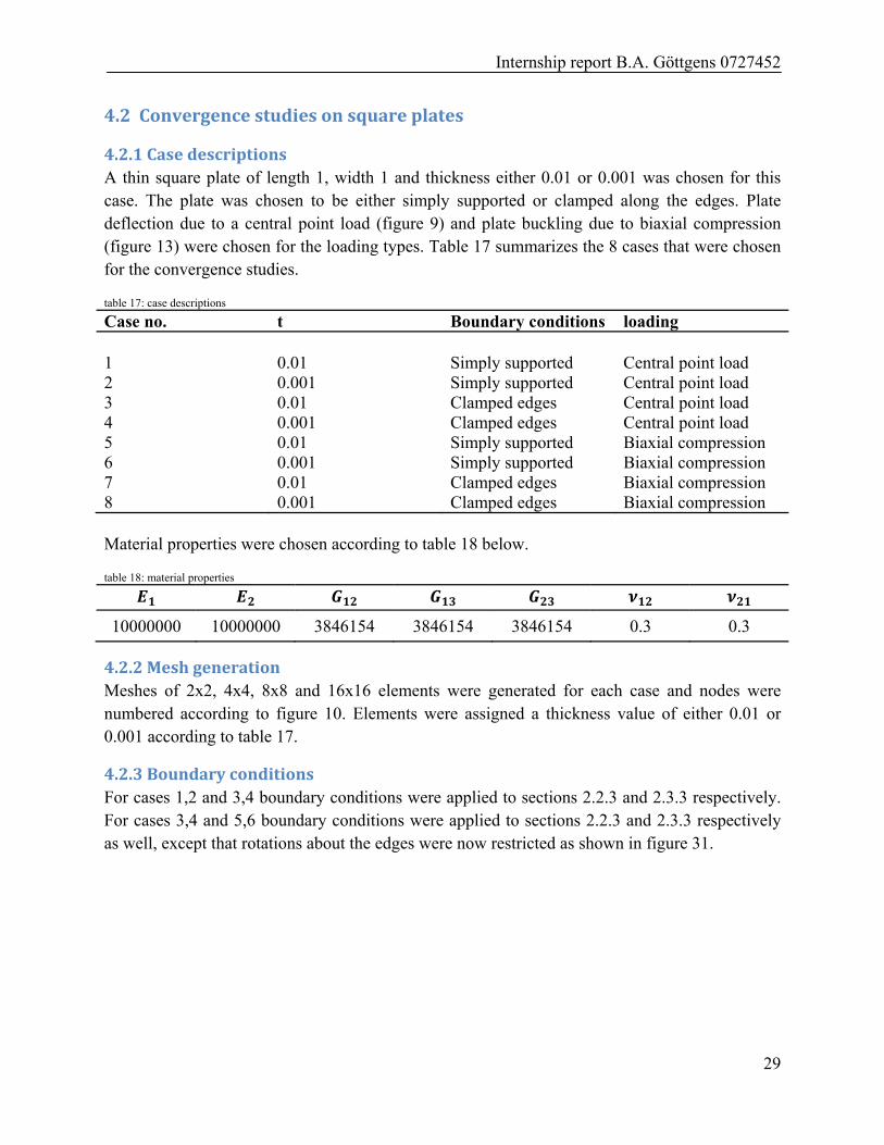
4.2.3BoundaryconditionsFor cases 1,2 and 3,4 boundary conditions were applied to sections 2.2.3 and 2.3.3 respectively. For cases 3,4 and 5,6 boundary conditions were applied to sections 2.2.3 and 2.3.3 respectively as well, except that rotations about the edges were now restricted as shown in figure 31.
Internship report B.A. Gӧttgens 0727452
30
figure 31: added constraints for the clamped edge boundary condition
4.2.4ClosedformsolutionsCases 1 and 2 were compared to (3). Cases 5 and 6 were compared to (5). Cases 3 and 4 can be compared to
0.005612
(11)
where
12 1
Unfortunately, no closed form solution was found to compare cases 7 and 8 to.
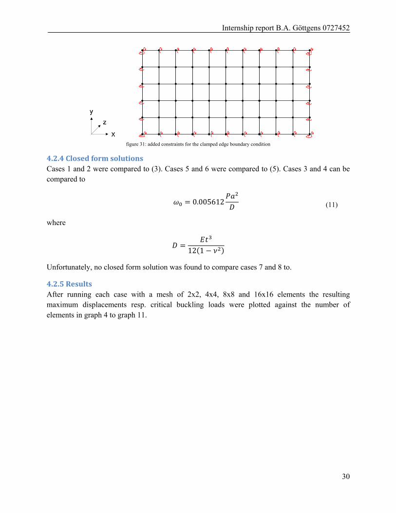
4.2.5ResultsAfter running each case with a mesh of 2x2, 4x4, 8x8 and 16x16 elements the resulting maximum displacements resp. critical buckling loads were plotted against the number of elements in graph 4 to graph 11.
Internship report B.A. Gӧttgens 0727452
31
graph 4: maximum displacement plotted against number of elements per side for case 1
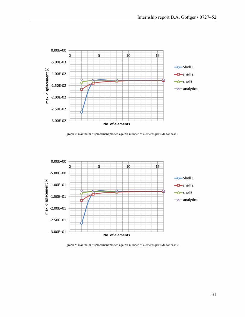
graph 5: maximum displacement plotted against number of elements per side for case 2
‐3.00E‐02
‐2.50E‐02
‐2.00E‐02
‐1.50E‐02
‐1.00E‐02
‐5.00E‐03
0.00E+00
0 5 10 15
max. d
isplacement [‐]
No. of elements
Shell 1
shell 2
shell3
analytical
‐3.00E+01
‐2.50E+01
‐2.00E+01
‐1.50E+01
‐1.00E+01
‐5.00E+00
0.00E+00
0 5 10 15
max. d
isplacement [‐]
No. of elements
Shell 1
shell 2
shell3
analytical
Internship report B.A. Gӧttgens 0727452
32
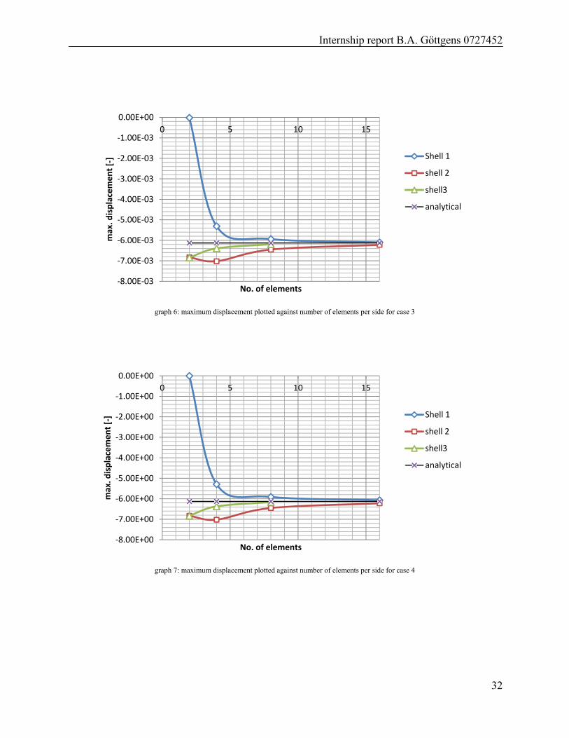
graph 6: maximum displacement plotted against number of elements per side for case 3
graph 7: maximum displacement plotted against number of elements per side for case 4
‐8.00E‐03
‐7.00E‐03
‐6.00E‐03
‐5.00E‐03
‐4.00E‐03
‐3.00E‐03
‐2.00E‐03
‐1.00E‐03
0.00E+00
0 5 10 15
max. d
isplacement [‐]
No. of elements
Shell 1
shell 2
shell3
analytical
‐8.00E+00
‐7.00E+00
‐6.00E+00
‐5.00E+00
‐4.00E+00
‐3.00E+00
‐2.00E+00
‐1.00E+00
0.00E+00
0 5 10 15
max. d
isplacement [‐]
No. of elements
Shell 1
shell 2
shell3
analytical
Internship report B.A. Gӧttgens 0727452
33
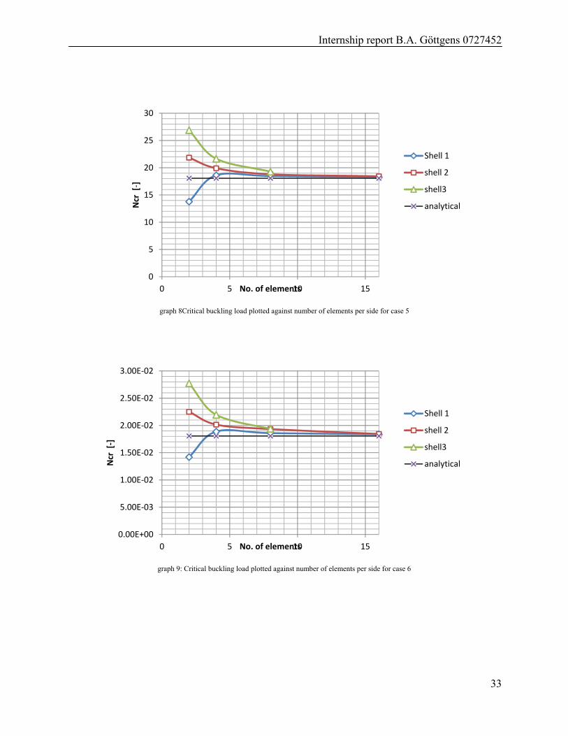
graph 8Critical buckling load plotted against number of elements per side for case 5
graph 9: Critical buckling load plotted against number of elements per side for case 6
0
5
10
15
20
25
30
0 5 10 15
Ncr [‐]
No. of elements
Shell 1
shell 2
shell3
analytical
0.00E+00
5.00E‐03
1.00E‐02
1.50E‐02
2.00E‐02
2.50E‐02
3.00E‐02
0 5 10 15
Ncr [‐]
No. of elements
Shell 1
shell 2
shell3
analytical
Internship report B.A. Gӧttgens 0727452
34
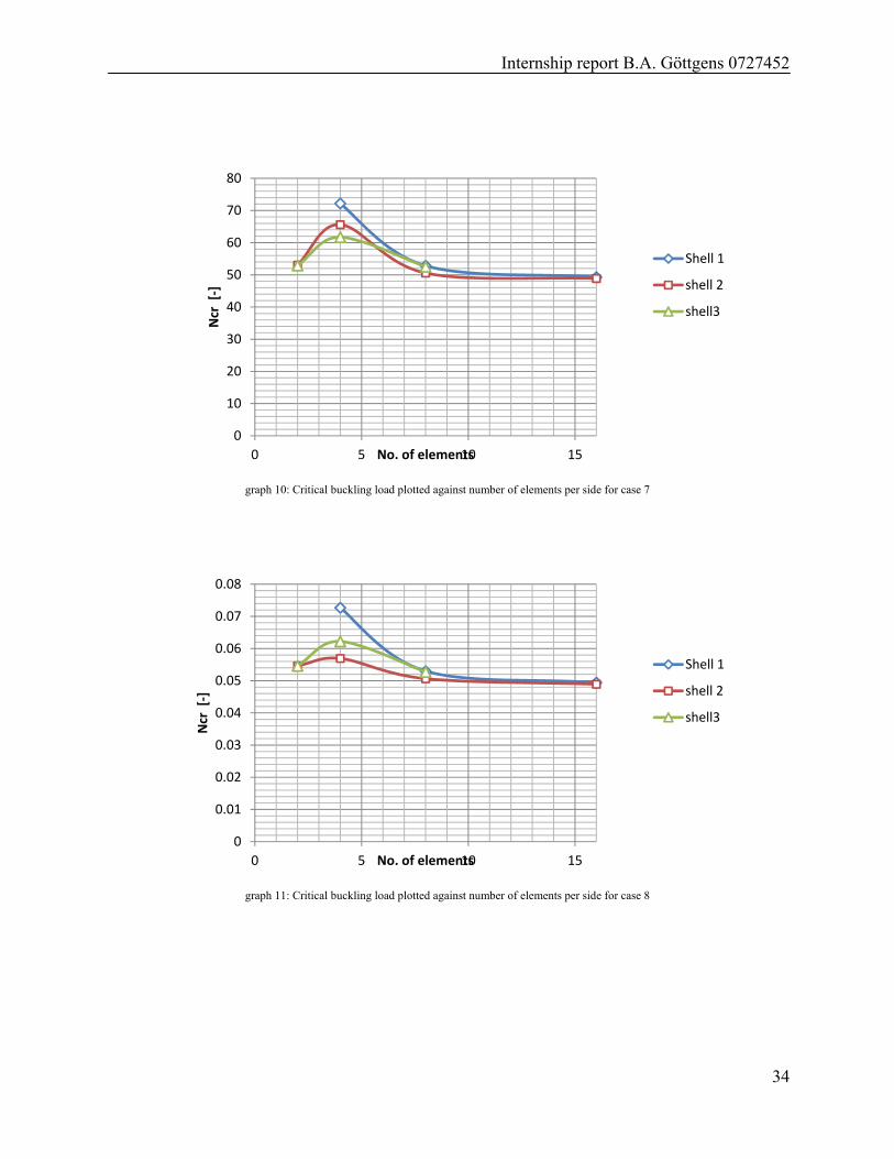
graph 10: Critical buckling load plotted against number of elements per side for case 7
graph 11: Critical buckling load plotted against number of elements per side for case 8
0
10
20
30
40
50
60
70
80
0 5 10 15
Ncr [‐]
No. of elements
Shell 1
shell 2
shell3
0
0.01
0.02
0.03
0.04
0.05
0.06
0.07
0.08
0 5 10 15
Ncr [‐]
No. of elements
Shell 1
shell 2
shell3
Internship report B.A. Gӧttgens 0727452
35
5ConclusionsFrom chapter 2, where the validation was performed with a shell element based on selective reduced integration (shell element 2) we can conclude that the tool generally performs adequately. However, for the case of non-square plate deflections the error made was unacceptably large and no explanation for this was found. In the case of non-square plate buckling the error was very large but can be explained by the closed form’s assumption on the buckled shape.
From chapter 3 we can conclude that laminate properties play an important role in the critical buckling loads of thin-walled beams and could even cause a transition from global to local buckling effects. Chapter 3 also illustrates that the assumption of lateral buckling behavior is not valid for any arbitrary thin-walled beam.
Although the numerical tool is computationally quite expensive, the method can clearly calculate correct critical applied loads. Perhaps a homogenization can be applied within the current commercially available software in order to provide more accurate results. Perhaps other ways can be thought of to include this numerical tool in order to consider local buckling effects.
From chapter 4 we can conclude that in the case of thin plate deflections, shell elements based on the twist-Kirchhoff theory (shell element 3) provide superior convergence compared to shell elements based on selective reduced integration (shell element 2). However for the case of thin plate buckling (and possibly thin-walled beam buckling) shell element 3 has no superior convergence rate. Due to the fact that mesh generation and computing time become very expensive it would not be advisable to apply shell element 3 to buckling problems.
Internship report B.A. Gӧttgens 0727452
36
Bibliography
[1] R. E. Erkmen, B.A. Gӧttgens, “Buckling analysis of thin-walled composite laminated members using a new shell element” Composite Structures, not yet published
[2] F. Brezzi, J.A. Evans, T.J.R Hughes, L.D. Marini, “New rectangular plate elements based on twist-Kirchhoff theory”, Comput. Methods Appl. Mech. Engrg. 200 (2011) 2547–2561
[3] J.N. Reddy, “Mechanics of laminated composite plates and shells: Theory and Analysis”, 2nd ed., CRC Press (2003) 202-209
[4] S.P. Timoshenko, S. Woinowsky-Krieger, “Theory of Plates and Shells, 2nd ed”, McGraw-Hill, New York, NY (1959)
[5] J.N. Reddy, “Mechanics of laminated composite plates and shells: Theory and Analysis”, 2nd ed., CRC Press (2003) 247-249
[6] S.P. Timoshenko, S. Woinowsky-Krieger, “Theory of Plates and Shells, 2nd ed”, McGraw-Hill, New York, NY (1959) 432
[7] R.E. Erkmen, M. Mohareb, “ Buckling analysis of thin-walled open members – A finite element formulation”, Thin-Walled Structures 46 (2008) 618–636
[8] A. Sapkás, L.P. Kollár, “Lateral-torsional buckling of composite beams”, International
Journal of Solids and Structures 39 (2002) 2939–2963
[9] N.S. Trahair, “Flexural–torsional buckling of structures” Boca Raton, FL, USA: CRC Press (1993)
Internship report B.A. Gӧttgens 0727452
37
Appendix1Derivationofstiffnessmatrices
Constitutive relations
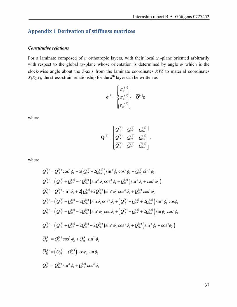
For a laminate composed of n orthotropic layers, with their local xy-plane oriented arbitrarily with respect to the global xy-plane whose orientation is determined by angle which is the
clock-wise angle about the Z-axis from the laminate coordinates XYZ to material coordinates X1X2X3, the stress-strain relationship for the kth layer can be written as
kx
k k ky
kxy
σ Q ε
where
11 12 16
12 22 26
16 26 66
k k k
k k k k
k k k
Q Q Q
Q Q Q
Q Q Q
Q ,
where
4 2 2 411 11 12 66 22cos 2 2 sin cos sink k k k k
k k k kQ Q Q Q Q
2 2 4 412 11 22 66 124 sin cos sin cosk k k k k
k k k kQ Q Q Q Q
4 2 2 422 11 12 66 22sin 2 2 sin cos cosk k k k k
k k k kQ Q Q Q Q
3 316 11 12 66 12 22 662 sin cos 2 sin cosk k k k k k k
k k k kQ Q Q Q Q Q Q
3 326 11 12 66 12 22 662 sin cos 2 sin cosk k k k k k k
k k k kQ Q Q Q Q Q Q
2 2 4 466 11 22 12 66 662 2 sin cos sin cosk k k k k k
k k k kQ Q Q Q Q Q
2 244 44 55cos sink k k
k kQ Q Q
45 55 44 cos sink k kk kQ Q Q
2 255 44 55sin cosk k k
k kQ Q Q
Internship report B.A. Gӧttgens 0727452
38
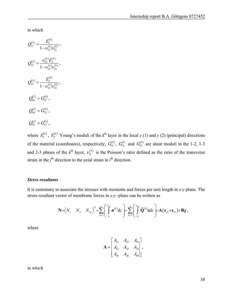
in which
1
11
12 211
kk
k k
EQ
,
12 2
12
12 211
k kk
k k
EQ
,
2
22
12 211
kk
k k
EQ
,
66 12
k kQ G ,
44 23
k kQ G ,
55 13
k kQ G ,
where 1
kE , 2
kE Young’s moduli of the kth layer in the local x (1) and y (2) (principal) directions
of the material (coordinates), respectively, 12
kG , 13
kG and 23
kG are shear moduli in the 1-2, 1-3
and 2-3 planes of the kth layer, kij is the Poisson’s ratio defined as the ratio of the transverse
strain in the jth direction to the axial strain in ith direction.
Stress resultants
It is customary to associate the stresses with moments and forces per unit length in x-y plane. The stress resultant vector of membrane forces in x-y -plane can be written as
1 1
T
1 1
d dk k
k k
z zn nk k
x y xy m Nk kz z
N N N z z
N σ Q ε A ε ε Bχ ,
where
11 12 16
12 22 26
16 26 66
A A A
A A A
A A A
A ,
in which
Internship report B.A. Gӧttgens 0727452
39
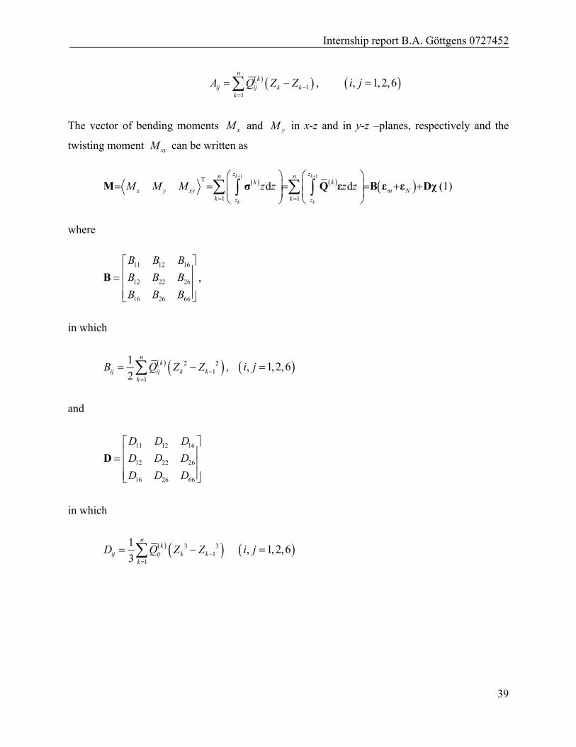
11
nk
ij ij k kk
A Q Z Z
, , 1,2,6i j
The vector of bending moments xM and yM in x-z and in y-z –planes, respectively and the
twisting moment xyM can be written as
1 1
T
1 1
d dk k
k k
z zn nk k
x y xy m Nk kz z
M M M z z z z
M σ Q ε B ε ε Dχ (1)
where
11 12 16
12 22 26
16 26 66
B B B
B B B
B B B
B ,
in which
2 21
1
1
2
nk
ij ij k kk
B Q Z Z
, , 1,2,6i j
and
11 12 16
12 22 26
16 26 66
D D D
D D D
D D D
D
in which
3 31
1
1
3
nk
ij ij k kk
D Q Z Z
, 1,2,6i j