APL: Autonomous Passive Localization for Wireless Sensors Deployed in Road Networks

IEEE INFOCOM 2008, Phoenix, AZ, USA

Jaehoon Jeong, Shuo Guo, Tian He and David DuComputer Science and Engineering, University of Minnesota

{jjeong,sguo,tianhe,du}@cs.umn.edu

April 16th, 2008

1

Problem Definition

Wireless SensorDeployment

Detection Timestamp

Target Detecting Sensors

2

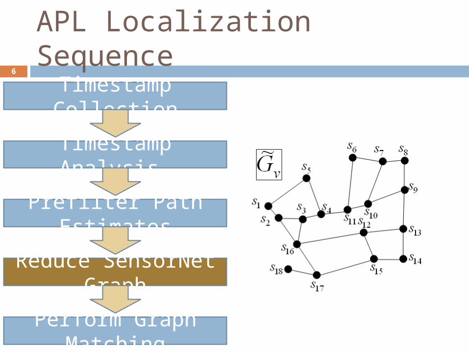
APL Localization Sequence3

Timestamp Analysis

Timestamp Collection

Prefilter Path Estimates

Reduce SensorNet Graph

Perform Graph Matching

APL Localization Sequence4

Timestamp Analysis

Timestamp Collection

Prefilter Path Estimates

Reduce SensorNet Graph

Perform Graph Matching

APL Localization Sequence5

Timestamp Analysis

Timestamp Collection

Prefilter Path Estimates

Reduce SensorNet Graph

Perform Graph Matching

APL Localization Sequence6

Timestamp Analysis

Timestamp Collection

Prefilter Path Estimates

Reduce SensorNet Graph

Perform Graph Matching

APL Localization Sequence7

Timestamp Analysis

Timestamp Collection

Prefilter Path Estimates

Reduce SensorNet Graph

Perform Graph Matching

SensorNetwork

Road Network

Matching

APL Localization Sequence8

Timestamp Analysis

Timestamp Collection

Prefilter Path Estimates

Reduce SensorNet Graph

Perform Graph Matching

APL Localization Sequence9

Timestamp Analysis

Timestamp Collection

Prefilter Path Estimates

Reduce SensorNet Graph

Perform Graph Matching

Isomorphic

APL Localization Sequence10

Timestamp Analysis

Timestamp Collection

Prefilter Path Estimates

Reduce SensorNet Graph

Perform Graph Matching

Matching

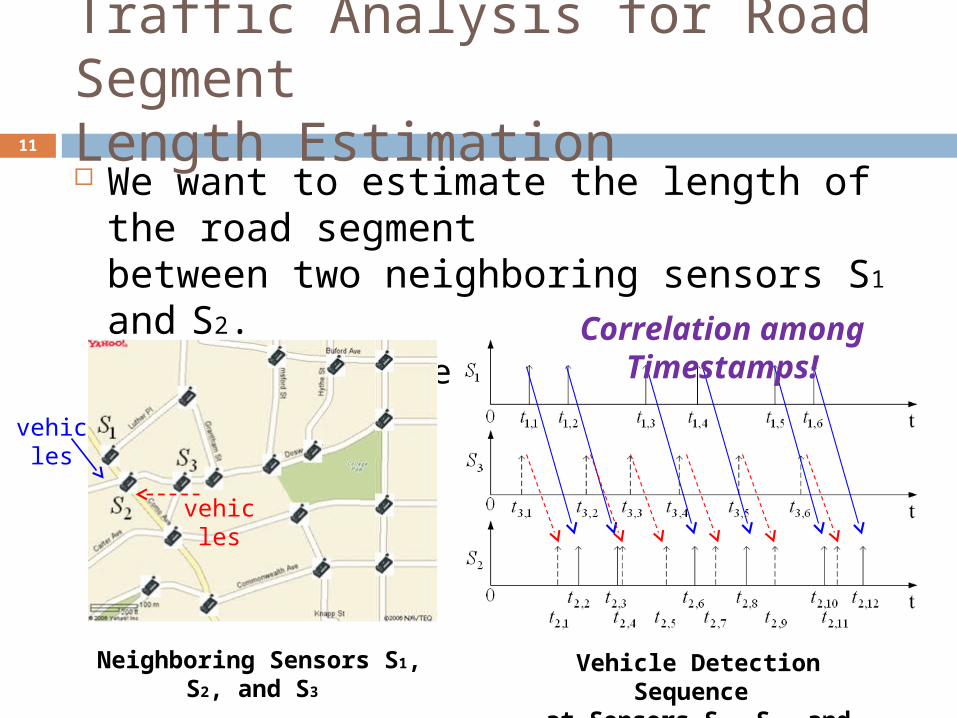
Traffic Analysis for Road SegmentLength Estimation We want to estimate the length of the road segment

between two neighboring sensors S1 and S2. There are three sensors S1, S2, and S3 as below:

Neighboring Sensors S1, S2, and S3 Vehicle Detection Sequence at Sensors S1, S2, and S3

11

Correlation among Timestamps!

vehicles

vehicles

Time Difference on Detection (TDOD)Operation

Time Difference On Detection(TDOD) for Sensors S1 and S2

Estimation of Movement Time through TDOD Operation

0 5 10 15 20 25 300

5

10

15

20

25

Time Difference [sec]

Fre

quen

cy (

Tim

e D

iffer

ence

Cou

nt)

Estimated Movement Time: 7.3 sec

m 7.10013.8*7.3V*TL Road Segment Length?

12

Comparison between Non-aggregation Method and Aggregation Method

0 5 10 15 20 25 300

2

4

6

8

10Non-aggregation Method

Time Difference [sec]

Fre

quen

cy

0 5 10 15 20 25 300

20

40

60

80Aggregation Method

Time Difference [sec]

Fre

quen

cyEstimated Movement Time

Estimated Movement Time

13

For Noise-Resilient Estimate,we compute Moving Average with

Time Difference Window of 10 seconds.

For Noise-Resilient Estimate,we compute Moving Sum with

Aggregation Window of 5 seconds.

0 5 10 15 20 25 300

2

4

6

8

10Non-aggregation Method

Time Difference [sec]

Fre

quen

cy

0 5 10 15 20 25 300

20

40

60

80Aggregation Method

Time Difference [sec]

Fre

quen

cyEstimated Movement Time

Estimated Movement Time

Aggregation Window

WrongEstimate

AccurateEstimate

Speed LimitV =50 km/h

Road LengthL =130 m

Movement TimeT = L/V=9.36 sec

26.8 sec

9.3 sec

Estimated Road LengthL’ =129.2 m

Outdoor Test for TDOD14

Test Road Network

Speed LimitV =64.4 km/h

Road (A, B)L =800 m

Movement TimeT = L/V= 44.7 sec

Speed LimitV =64.4 km/h

Road (B, C)L =900 m

Movement TimeT = L/V= 50.3 sec

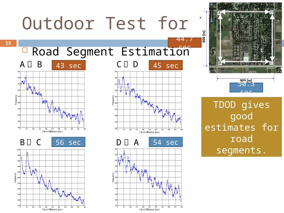
Outdoor Test for TDOD15

Road Segment Estimation

0 50 100 150 200 250 300 350 400 450 500200

250

300

350

400

450

500

550

600

650

Time Difference [sec]

Fre

quen

cy

A ՞ B 43 sec

0 50 100 150 200 250 300 350 400 450 500200

250

300

350

400

450

500

550

600

650

Time Difference [sec]

Fre

quen

cy

C՞ D 45 sec

0 50 100 150 200 250 300 350 400 450 500500

600

700

800

900

1000

1100

1200

1300

1400

1500

Time Difference [sec]

Fre

quen

cy

B՞ C 56 sec

0 50 100 150 200 250 300 350 400 450 50080

100

120

140

160

180

200

220

240

260

280

Time Difference [sec]

Fre

quen

cy

D՞ A 54 sec

44.7 sec

50.3 sec

TDOD gives good estimates for road

segments.

Path Estimate vs. Road Segment Estimate16

95 sec 95 sec

A ՞ B՞ C B՞ C՞ D

0 50 100 150 200 250 300 350 400 450 500200

250

300

350

400

450

500

550

600

Time Difference [sec]

Fre

qu

en

cy

A ՞ B՞ C 37 sec

0 50 100 150 200 250 300 350 400 450 500200

250

300

350

400

450

500

550

600

650

Time Difference [sec]

Fre

qu

en

cy

B՞ C՞ D 52 sec

TDOD cannot give good estimates for

paths.

Path estimate has a large deviation

per traffic measure.

Procedure of Prefiltering for Virtual Graph

(a) Road Sensor Network (b) Virtual Topology for Sensors

(c) Virtual Graph after Prefiltering based on Relative Deviation Error

(d) Virtual Graph after Prefiltering based on Minimum Spanning Tree

17

Isomorphic

Graph Matching

Now, we have a virtual graph whose subgraph is isomorphic to the real graph corresponding to the road network.

(a) Road Sensor Network

(b) Virtual Topologyof Wireless Sensors

(c) Virtual Graphfor Sensor Network

18

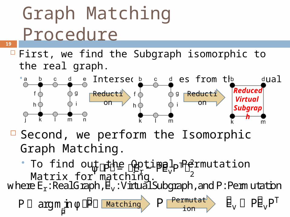
Graph Matching Procedure

First, we find the Subgraph isomorphic to the real graph. To find out Intersection Nodes from the Virtual Graph.

Second, we perform the Isomorphic Graph Matching. To find out the Optimal Permutation Matrix for matching.

Reduction Reduction

ϕሺPሻ= ฮEr − PE෩vPTฮ22 where Er: Real Graph, E෩v: Virtual Subgraph, and P: Permutation P ՚ argminP ϕ൫P൯ E v ՚ PE෩vPT Matching

ReducedVirtual

Subgraph

19

P Permutation

Graph Matching Example

Virtual Graph Virtual Subgraph

Road Network Real Graph

G෩v and Gr Isomorphic

Reduction

AbstractionPermutation

Matrix P

Mat

chin

g

20

Node Location Identification

Localization of Intersection Nodes We have localized Intersection Nodes with Permutation

Matrix P.

Localization of Non-intersection Nodes Let Gv = (Vv, Ev) be the virtual graph. Beginning from an intersection node u

in Ev, we create a path from u to another intersection node v such as

Virtual Graph

u ՜ a1 ՜ a2 ՜ …՜ am ՜ v

21

Real Graph

Node Localization Done!

u v

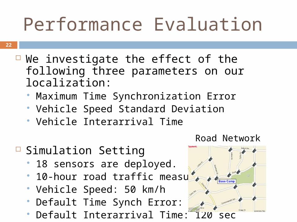
Performance Evaluation

We investigate the effect of the following three parameters on our localization: Maximum Time Synchronization Error Vehicle Speed Standard Deviation Vehicle Interarrival Time

Simulation Setting 18 sensors are deployed. 10-hour road traffic measurement Vehicle Speed: 50 km/h Default Time Synch Error: 0.01 sec Default Interarrival Time: 120 sec

Road Network

22

Performance Comparison between Road Segment Estimation Methods Maximum Time Synchronization Error

Up to 0.3-second time-synch error, 0% localization error rate can be achieved.

Vehicle Speed Standard Deviation Up to 10 km/h vehicle-speed deviation,

0% localization error rate can be achieved.

Vehicle Interarrival Time For the interarrival time greater than 1 second,

0% localization error rate can be achieved.

23

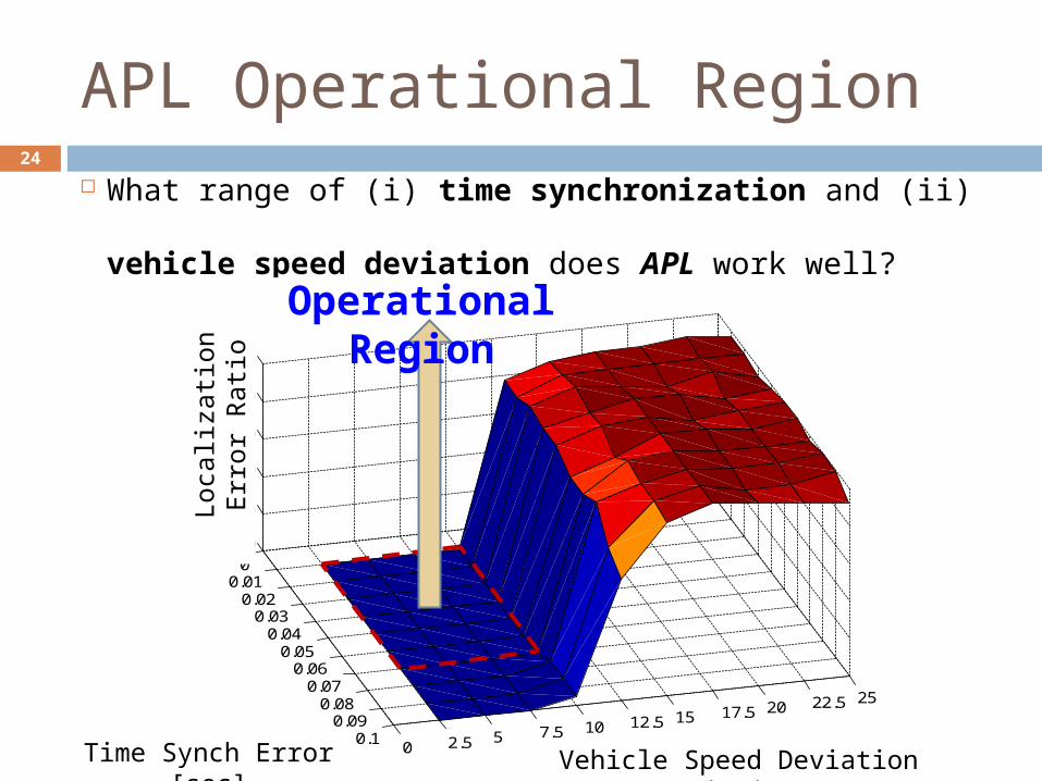
APL Operational Region

What range of (i) time synchronization and (ii) vehicle speed deviation does APL work well?

00.01

0.020.03

0.040.05

0.060.07

0.080.09

0.10 2.5 5 7.5 10 12.5 15 17.5 20 22.5 25

0

0.2

0.4

0.6

0.8

1

Vehicle Speed Deviation [km/h]Maximum Time Sync Error [sec]

Localiz

ation E

rror

Ratio

Vehicle Speed Deviation [km/h]Time Synch Error [sec]

Loc

aliz

atio

n E

rror

Rat

io

24

Operational Region

Conclusion

In sparse sensor networks over road networks, sensors cannot effectively obtain (i) pair-wise ranging distance or (ii) connectivity information. Our Autonomous Passive Localization (APL) works

well under realistic scenarios With Vehicle-detection timestamps and With Road map of target area.

As next step, we will perform the test of APL systemin real road networks with Motes such as XSM.

25

Q & A26