Embed Size (px)
Citation preview
A Practical Introduction to
APL 1 &
APL 2
by
Graeme Donald Robertson
. . TRAINING THAT WORKS . . .
Date: ..................................
Place: ...................................
Instructor: ...................................................................................
Student(s): ...................................................................................
.......................................................................................................................
.......................................................................................................................
.......................................................................................................................
.......................................................................................................................
.......................................................................................................................
A Practical Introduction to APL 1 & APL 2
2
ROBERTSON (Publishing)
15 Little Basing, Old Basing,
Basingstoke, RG24 8AX, UK.
Copyright © Graeme Donald Robertson 2004-2008
This publication may be used, reproduced, stored in a
retrieval system, or transmitted in any form or by any
means, electronic, mechanical, photocopying, recording
or otherwise, without the permission of the publisher.
This document is distributed subject to the condition that
it shall not, by way of trade or otherwise, be sold or hired
out without the publisher’s prior consent. It may however
be used in APL classes and circulated in any form of
binding or cover with a similar condition, including this
condition, being imposed on the subsequent owner.
First edition published March 2004 as APL1&2.PDF
Second edition published September 2004 as APL1_2.PDF Third edition published January 2008 as APL1&2.PDF
ISBN 0 9524167 1 9
Conduct of this 2 day course:
After short introductions, the student group is invited to divide up into pairs.
Each pair works on one computer/terminal for the duration of the course.
Each pair is given the first lesson and asked to work through it on their computer at their own pace.
Pairs are encouraged to help each other with new concepts and difficulties as they arise and to experiment on the
computer with any ideas which they think they can express in APL statements.
Tuition is given when problems cannot be resolved by the pair. Questions may be answered directly on matters of
fact, or indirectly by way of a suggestion as to how the problem might be tackled.
Each day covers about 7 lessons, depending upon the pace of each pair.
There is no pressure to complete all lessons (remaining notes are given out at the end of the course).
At the discretion of the tutor, lessons may be skipped or assigned for private study after the course has ended.
Short synopses are given (with an overhead projector or white board) at suitable intervals throughout the course to the
group as a whole.
A Practical Introduction to APL 1 & APL 2
3
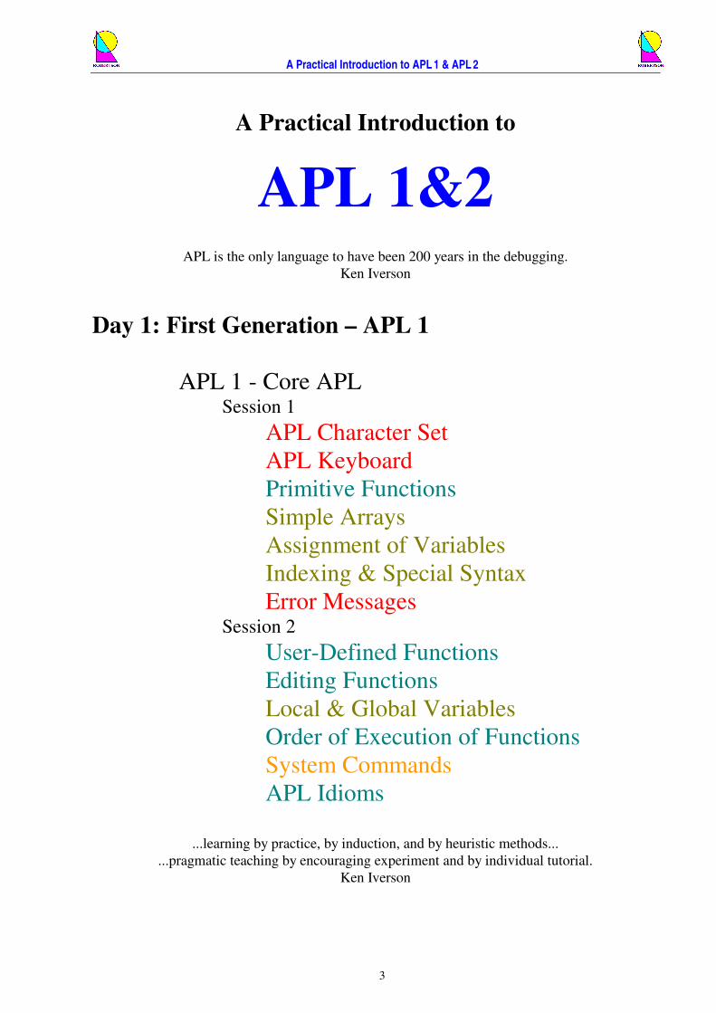
A Practical Introduction to
APL 1&2
APL is the only language to have been 200 years in the debugging.
Ken Iverson
Day 1: First Generation – APL 1
APL 1 - Core APL Session 1
APL Character Set
APL Keyboard
Primitive Functions
Simple Arrays
Assignment of Variables
Indexing & Special Syntax
Error Messages Session 2
User-Defined Functions
Editing Functions
Local & Global Variables
Order of Execution of Functions
System Commands
APL Idioms
...learning by practice, by induction, and by heuristic methods...
...pragmatic teaching by encouraging experiment and by individual tutorial.
Ken Iverson
A Practical Introduction to APL 1 & APL 2
4
L E S S O N 0
Why Learn APL?
APL is a high-level, general-purpose, intuitive programming language which is designed to be
easy on the programmer even if consequently hard on the computer - through power, not
inefficiency.
APL has its own special character set of around 200 alphabetic characters and symbols. Although
the APL symbols might appear illegible and unintelligible, each individual symbol performs a
specific task making programs very concise. APL is A Programming Language which is
essentially simple and easy to learn, and APL is interactive making it possible to experiment with
different ideas while developing solutions.
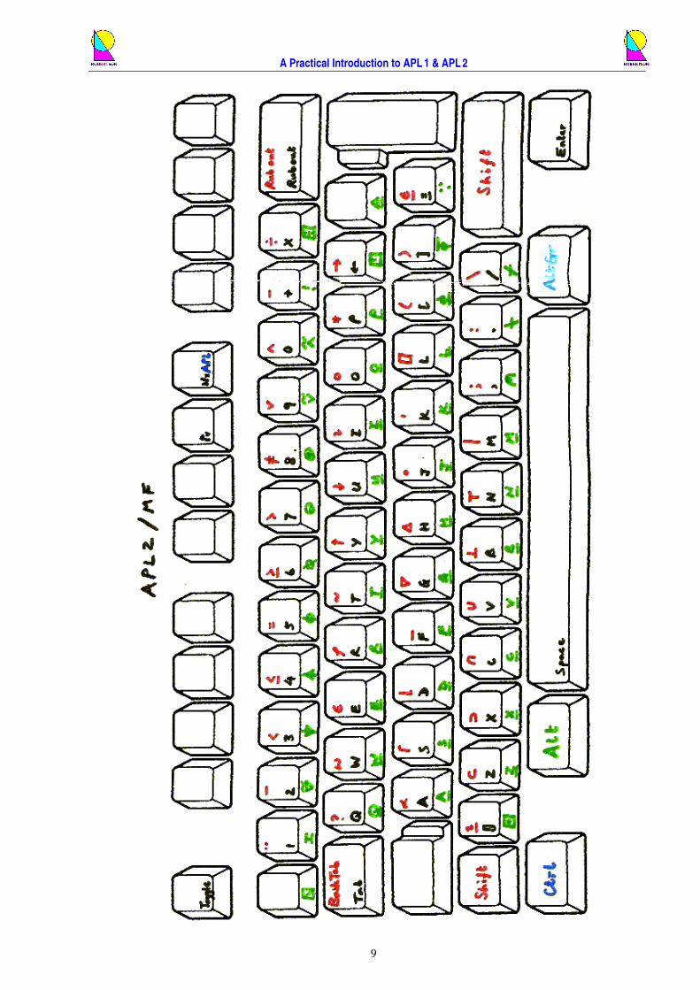
Getting to Know Your APL Keyboard
Your computer should be set up already so that an APL session is visible and has the focus.
Typing on your keyboard should cause characters to be displayed on your screen. Try typing
something. When you come across a new symbol, or key combination, write it on the supplied
blank keyboard. This will help you quickly to become familiar with the new APL key layout.
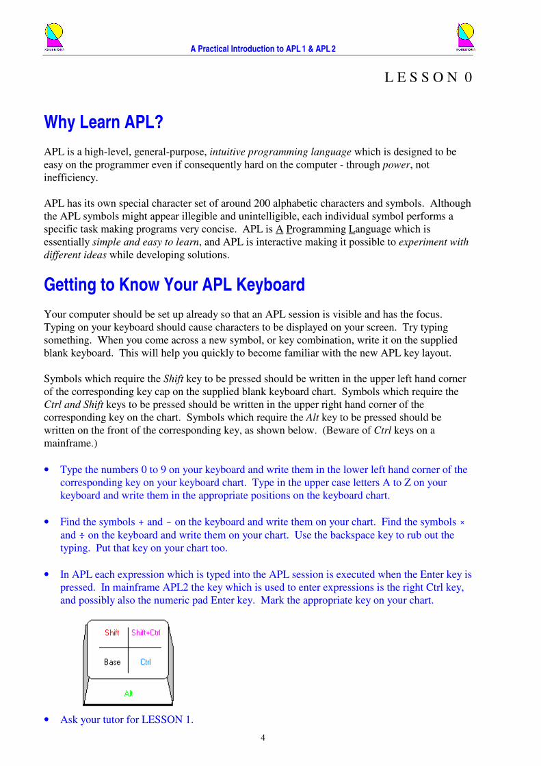
Symbols which require the Shift key to be pressed should be written in the upper left hand corner
of the corresponding key cap on the supplied blank keyboard chart. Symbols which require the
Ctrl and Shift keys to be pressed should be written in the upper right hand corner of the
corresponding key on the chart. Symbols which require the Alt key to be pressed should be
written on the front of the corresponding key, as shown below. (Beware of Ctrl keys on a
mainframe.)
• Type the numbers 0 to 9 on your keyboard and write them in the lower left hand corner of the
corresponding key on your keyboard chart. Type in the upper case letters A to Z on your
keyboard and write them in the appropriate positions on the keyboard chart.
• Find the symbols + and - on the keyboard and write them on your chart. Find the symbols ×
and ÷ on the keyboard and write them on your chart. Use the backspace key to rub out the
typing. Put that key on your chart too.
• In APL each expression which is typed into the APL session is executed when the Enter key is
pressed. In mainframe APL2 the key which is used to enter expressions is the right Ctrl key,
and possibly also the numeric pad Enter key. Mark the appropriate key on your chart.
• Ask your tutor for LESSON 1.

A Practical Introduction to APL 1 & APL 2
5
A Practical Introduction to APL 1 & APL 2
6
L E S S O N 1
Simple Arithmetic Expressions
Go at your own pace. Experiment. Try to work it out. Think. Talk about it.
• Use APL to add any two numbers together. Check the result. For example, type
65.35 + 35.65 101
Hint: Hit the Enter key when you are ready to execute the line containing the cursor.
Notice how, in immediate execution mode, APL indents the cursor 6 spaces to indicate that it is
ready to accept the next line of user input. Everything which has been input by the user is
indented by 6 spaces, and is coloured green in mainframe APL2. Output from the computer
starts at the left hand margin and is coloured red, as are error lines.
• Type the following two lines into your session and explain the results.
14 - 9 5 - 7 ¯7
Notice the distinction between the negate function (-) and the negative sign, or high minus
symbol, (¯), which is an intrinsic part of a number, like the decimal point.
Symbols such as - and + can be used either with a right argument (which is called the monadic
or prefix case) or with a left and right argument (which is called the dyadic or infix case). Thus
the hyphen symbol can be used monadically to mean negate or dyadically to mean minus, or
subtract. Write the new high minus symbol on your keyboard chart.
The plus and minus signs were introduced by the German mathematician Johann Widmann in
1489 to signify addition and subtraction. Dyadic deployment of the symbols is now familiar to
everyone.
APL has many such powerful primitive functions which allow complex computations to be done
very easily. Primitive functions follow the principle of one symbol per mathematical operation.
• Experiment to see if you can deduce the monadic and dyadic meanings of the symbols
× ÷ | — ˜ * µ ! both by applying simple numeric arguments, and by inference from
the form of the symbol itself.
The times sign was introduced by the English mathematician who invented the slide rule;
William Oughtred (1575 - 1660). Its use to signify multiplication is now familiar to everyone
who has been exposed to the language of elementary algebra. Most computer languages use * to
indicate multiplication. Algebraists use a variety of alternative ways to indicate multiplication:
a×b or a.b or ab. APL consistently uses ×. "APL is the only [computer] language to have been
two hundred years in the debugging," says Iverson.
A Practical Introduction to APL 1 & APL 2
7
APL is derived from mathematical notation. It did not appear from the standard evolutionary
origins of most other computer languages. APL crystallized from an unconstrained theoretical
notation (Iverson notation) when it was realized that it could be executed on a computer. "I
wasn't trying to design or implement a language for a machine," confessed Iverson.
The monadic meanings of × ÷ | — ˜ * µ and ! are direction, reciprocal, magnitude,
ceiling, floor, exponential, natural logarithm and factorial respectively, and dyadic meanings
multiply, divide, residue, maximum, minimum, power, logarithm and binomial respectively.
• Investigate the monadic meaning of + Experiment with any suggestive arguments! ;-)
The result of one expression can be used as the argument to another function.
• Try some compound expressions such as
3 × 4 + 6 30
and
(3 × 4) + 6 18
Hence explain the result of the expression
14 - 6 - 5 - 3 - 7 17
Beyond BIDMAS. Remember BIDMAS (or BODMAS)? It tells you the order of precedence in
simple arithmetic expressions – brackets first, then indices (or of), division, multiplication,
addition and finally subtraction. APL, on the other hand, does not assume any special order of
precedence between functions. Execution simply proceeds from right to left unless you use
parentheses (round brackets) to control the order of execution. All APL functions have equal
priority. This basic “right-to-left” grammatical rule applies to dyadic functions and monadic
functions alike in APL. (It’s a bit like the rule in English that the object of a sentence comes after
the verb.)
Rule 1: The right argument of any function, monadic or dyadic, is the result of the entire
expression immediately to its right.
Some functions take boolean arguments and return boolean results.
• Reading 1 as true and 0 as false, verify the truth values of these expressions.
1 Ÿ 1 1 1 ^ (0 ^ 1) Ÿ 1 Ÿ 0 1 ~ 0 Ÿ ~ 0
0
A Practical Introduction to APL 1 & APL 2
8
These invoke the simple logical functions: and (^), or (Ÿ) and not (~).
• Some functions take numeric arguments and return boolean results. Verify the results of
20.5 = 41 ÷ 2 1 101 < 200 - 100 0 27.3 > 39.31 0
These introduce binary relational functions: equals (=), less-than (<) and greater-than (>).
• Trigonometric functions are implemented via the dyadic circle function. A left argument of 1
returns the sine of the right argument. Assess the result of
1 ± 3.14159 0.000002654
knowing that Sin(π) is zero. A left argument of 2 returns the cosine, 3 returns the tangent.
The left argument of the circle function may be an integer between 12 and -12 representing
various standard pythagorean, trigonometric, hyperbolic and complex number functions.
• Explore a few examples. Find the meaning of the monadic circle function.
• Type the following line into your session and execute it a few times.
? 6 5
What do you think the results indicate about the meaning of roll (?)? ☺
• Try some more adventurous examples of the application of Rule 1.
˜0.5+3.23 3 —¯0.5+3.23 3 ˜¯3.5—¯8.2 4 3.2|¯4.3 2.1 ((?5)ˆ?8)Ÿ(?5)‰?8 1 (~1Š0‹1)=1ˆ0.2ˆ3ˆ4 0 (2!6)=(!6)÷(!2)×!4
1 ((3×4)=*(µ3)+µ4)^(3÷4)=*(µ3)-µ4 1 • Ask your tutor for LESSON 2.
A Practical Introduction to APL 1 & APL 2
9
A Practical Introduction to APL 1 & APL 2
10
L E S S O N 2
Names, Lists & Literals
Numbers and results of expressions can be assigned to names. The left assignment arrow („) may
be read as gets or is-assigned or simply is.
• Enter the following statements (or sentences), noting that * means power and × means times,
INTEREST „ 0.09 YEARS „ 6 VALUE„500×(1+INTEREST)*YEARS
• Type in the name of a variable and hit the Enter key to display the contents of the variable in
the session.
VALUE 838.6
Generalized Scalar Functions. Some functions that take single numbers (scalar) arguments
have well defined behaviour when the arguments are extended to lists of numbers (vector).
• Execute the line
1 2 3 + 4 6 8 5 8 11
and explain the result.
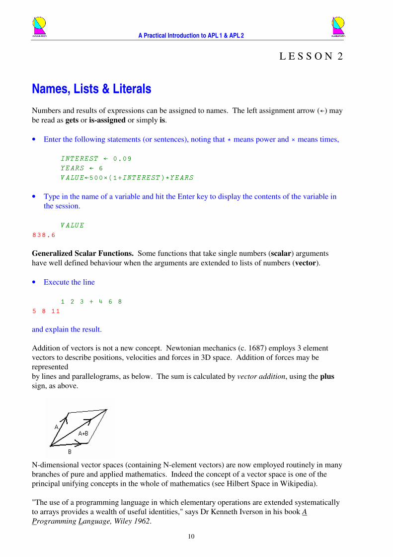
Addition of vectors is not a new concept. Newtonian mechanics (c. 1687) employs 3 element
vectors to describe positions, velocities and forces in 3D space. Addition of forces may be
represented
by lines and parallelograms, as below. The sum is calculated by vector addition, using the plus
sign, as above.
N-dimensional vector spaces (containing N-element vectors) are now employed routinely in many
branches of pure and applied mathematics. Indeed the concept of a vector space is one of the
principal unifying concepts in the whole of mathematics (see Hilbert Space in Wikipedia).
"The use of a programming language in which elementary operations are extended systematically
to arrays provides a wealth of useful identities," says Dr Kenneth Iverson in his book A
Programming Language, Wiley 1962.

A Practical Introduction to APL 1 & APL 2
11
APL adopts this element-by-element approach to vector addition and generalises it to many
standard mathematical functions, taking dyadic plus and monadic negate as role models, or
templates.
• Check the results of
- 3 4 5 ¯3 ¯4 ¯5 - 3 4 ¯5 4 6 5.0 ¯8.567 ¯3 ¯4 5 ¯4 ¯6 ¯5 8.567 1 2 3 × 2 ¯2 2 2 ¯4 6 45 ¯3 2 2.33 + 99 7 4 0.4 144 4 6 2.73
• Explore other expressions, using lists of numbers as arguments to the primitive scalar
functions represented by symbols + - × ÷ | — ˜ * µ ± !
Scalar Extension. If one of the arguments of a scalar dyadic function is a scalar and the other is
a vector (or list) then the scalar is automatically extended to have the same length as the vector.
• Enter
1 ± .1 .2 .3 0.09983 0.1987 0.2955
• Compare with
1 1 1 ± .1 .2 .3 0.09983 0.1987 0.2955
and
1 2 3 ± .1 .2 .3 0.09983 0.9801 0.3093
Otherwise, if the arguments have incompatible lengths then a LENGTH ERROR is reported.
• Try to execute the following line.
1 2 ± .1 .2 .3
Literals. Variables can be assigned to lists of literal characters as well as to lists of numbers.
Character strings have to be enclosed inside APL quotes in order to distinguish literal characters
from defined names or simple numerics.
• Enter your name and web address, e.g.
NAME„'DEBBIE ROBERTSON' ADDRESS„'APL4.NET'
A Practical Introduction to APL 1 & APL 2
12
The dyadic structural functions catenate (,) take (†) and drop (‡), and the monadic structural
function reverse (²), can be used on any list of numbers or characters to produce a new related
list.
• Try
²NAME
NOSTREBOR EIBBED 7†NAME DEBBIE E„(6†NAME),'@',ADDRESS E [email protected]
• Monadic use of Greek letter rho (function shape) returns the number of elements in the vector
NAME. Check the result of
½NAME 16
• Dyadic rho (reshape) returns the right argument reshaped to have exactly the number of
elements specified by the left argument. Try
4½ADDRESS APL4 40½ADDRESS APL4.NETAPL4.NETAPL4.NETAPL4.NETAPL4.NET ²50½NAME,' ' NOSTREBOR EIBBED NOSTREBOR EIBBED NOSTREBOR EIBBED
The shape of a vector is the number of elements in the list.
• Type
½NUMS„56 87 75 80 79 86 84 90 8 ½CHARS„'56 87 75 80 79 86 84 90' 23
Literal digits can be converted into numbers using the very powerful execute (–) function (which
is said to make APL ‘self-conscious’) and numbers can be converted into characters using the
very useful format (•) function.
• Explain the results of
½•NUMS 23 CHARS=•NUMS 1 1 1 1 1 1 1 1 1 1 1 1 1 1 1 1 1 1 1 1 1 1 1

A Practical Introduction to APL 1 & APL 2
13
½–CHARS 8 NUMS=–CHARS 1 1 1 1 1 1 1 1 CHARS,•NUMS 56 87 75 80 79 86 84 9056 87 75 80 79 86 84 90 –(3×5)½'NUMSª' 56 87 75 80 79 86 84 90 56 87 75 80 79 86 84 90 56 87 75 80 79 86 84 90
The diamond symbol (ª) is not a function. It is a statement separator. You might not be able to
find it on your APL2 mainframe keyboard. However, diamond is an example of an overstruck
character – from the days when space for characters was scarce. A diamond can be input using
the three consecutive symbols <_> where _ is the printable backspace. This requires that you
first type the command
)PBS ON
in APL2, or switch to replace mode via the Insert key in Dyalog APL.
Interval (¼) can be used to generate any uniformly spaced range of numbers.
The monadic meaning of the iota character (¼) is a function called interval or index generator. It
takes a scalar argument and returns a vector result.
• Try
¼9 1 2 3 4 5 6 7 8 9 ¼19 1 2 3 4 5 6 7 8 9 10 11 12 13 14 15 16 17 18 19 ¯1+(¼19)÷10 ¯0.9 ¯0.8 ¯0.7 ¯0.6 ¯0.5 ¯0.4 ¯0.3 ¯0.2 ¯0.1 0 0.1 0.2 0.3 0.4 0.5 0.6 0.7 0.8 0.9 • Experiment with examples like
¯0.3×8-¼15 ¯2.1 ¯1.8 ¯1.5 ¯1.2 ¯0.9 ¯0.6 ¯0.3 0 0.3 0.6 0.9 1.2 1.5 1.8 2.1 • Now try
¯1+(¼99)÷50 or
¯1+(¼9999)÷5000

A Practical Introduction to APL 1 & APL 2
14
• Use the appropriate keystroke (usually Ctrl+C on a mainframe keyboard or Ctrl+Break on a
PC) to interrupt execution of lengthy or verbose operations. Write this important key
combination on your keyboard chart. Learn to interrupt without compunction. Waiting for a
rogue function to finish may be very expensive on a mainframe. You control the computer
now.
APL primitive functions appear atomic in the sense that they never stop half way through. They
either finish completely or appear not to have started at all. Therefore breaking an APL process
always leaves the processing stack at a definite given point in an APL program.
APL idioms are commonly used combinations of tokens. They are phrases that are immediately
recognised by APL programmers when reading APL code. A simple example of an idiom is
¼½NUMS 1 2 3 4 5 6 7 8
which returns a count of the elements in the vector NUMS.
• Propose a use for this idiom:
(1‡NUMS)-(¯1‡NUMS) 31 ¯12 5 ¯1 7 ¯2 6
Note the occasional judicious use of redundant parentheses to enhance readability.
• Experiment with dyadic functions ½ † and ‡ using scalar (single) integer left arguments
and vector (list) numeric (or character) right arguments. Note, in particular, the shape of the
arguments and the shape of the results.
• Write an expression which rounds a number of pennies to the nearest 12p. Andrew, James,
Charles and Marcus each have a building society account: these contain £5,081.09,
£11,954.55, £812.97 and £6,241.00 respectively. Each account has a different annual interest
rate: 4.1%, 3.5%, 2.6% and 3.25%. Write an expression which returns the interest on each
account. Write another expression which returns how much each person could have at the
end of ten years of saving, to the nearest 12p?

A Practical Introduction to APL 1 & APL 2
15
L E S S O N 3
Indexing Non-Scalar Arrays
In a simple and intuitive manner, square brackets [ ] are used to select items from a list.
• Enter
NUMS[3 2] 75 87 (²¼99)[NUMS] 44 13 25 20 21 14 16 10 (33 44 55 66)[3 2 3 3 1] 55 44 55 55 33 'scarlet'[1 6 2 4 6 7] secret
The shape of the result is the shape of the index. If no index is included within the brackets
(elided index) then the whole vector is returned. e.g.
NUMS[] 87 75 80 79 86 84 90
• Use bracket indexing to select the smallest and largest elements from the vector
A „ ? 100 ½ 1000
Hint: Monadic grade-up (“), applied to argument A returns the permutation vector which would
sort A in ascending order.
Matrices. We have generalised the arguments of functions from scalars to vectors, or lists. Now
we generalise further to matrices, or tables.
When the concept of a matrix of numbers is first encountered in mathematics it can appear quite
forbidding, but they have many uses. For example, they form the bases of representations of
continuous groups which have many deep applications in science. We here consider a matrix
simply as a rectangular table of numbers or characters.
In order to create a vector we may use the dyadic reshape function (½), with a single numeric left
argument, to produce a list of that length containing elements taken consecutively from the right
argument. In order to create a matrix we may use the reshape function with a two element
numeric vector left argument to produce a table which has that number of rows and columns.
• Examine the displayed output from
3 4 ½ 999 999 999 999 999 999 999 999 999 999 999 999 999
A Practical Introduction to APL 1 & APL 2
16
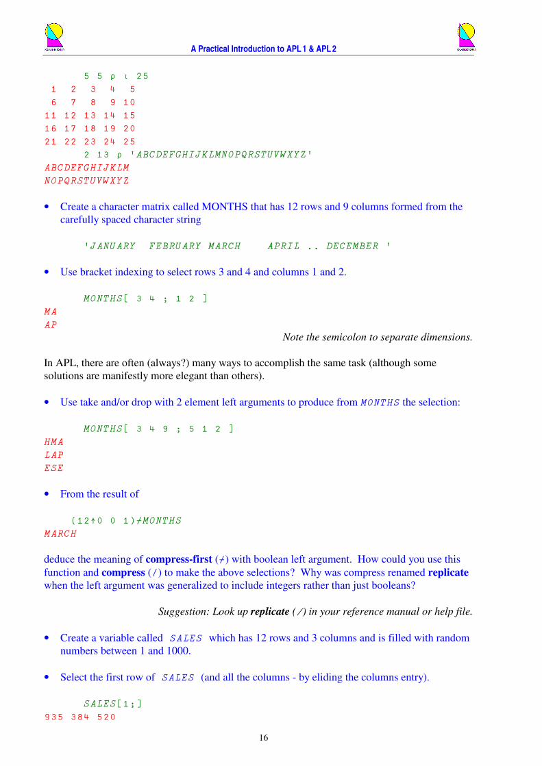
5 5 ½ ¼ 25 1 2 3 4 5 6 7 8 9 10 11 12 13 14 15 16 17 18 19 20 21 22 23 24 25 2 13 ½ 'ABCDEFGHIJKLMNOPQRSTUVWXYZ' ABCDEFGHIJKLM NOPQRSTUVWXYZ
• Create a character matrix called MONTHS that has 12 rows and 9 columns formed from the
carefully spaced character string
'JANUARY FEBRUARY MARCH APRIL .. DECEMBER '
• Use bracket indexing to select rows 3 and 4 and columns 1 and 2.
MONTHS[ 3 4 ; 1 2 ] MA AP
Note the semicolon to separate dimensions.
In APL, there are often (always?) many ways to accomplish the same task (although some
solutions are manifestly more elegant than others).
• Use take and/or drop with 2 element left arguments to produce from MONTHS the selection:
MONTHS[ 3 4 9 ; 5 1 2 ] HMA LAP ESE
• From the result of
(12†0 0 1)šMONTHS MARCH
deduce the meaning of compress-first (š) with boolean left argument. How could you use this
function and compress (/) to make the above selections? Why was compress renamed replicate
when the left argument was generalized to include integers rather than just booleans?
Suggestion: Look up replicate (/) in your reference manual or help file.
• Create a variable called SALES which has 12 rows and 3 columns and is filled with random
numbers between 1 and 1000.
• Select the first row of SALES (and all the columns - by eliding the columns entry).
SALES[1;] 935 384 520
A Practical Introduction to APL 1 & APL 2
17
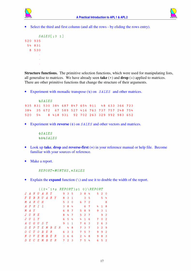
• Select the third and first column (and all the rows - by eliding the rows entry).
SALES[;3 1] 520 935 54 831 8 530 · · ·
Structure functions. The primitive selection functions, which were used for manipulating lists,
all generalise to matrices. We have already seen take (†) and drop (‡) applied to matrices.
There are other primitive functions that change the structure of their arguments.
• Experiment with monadic transpose (³) on SALES and other matrices.
³SALES 935 831 530 384 687 847 654 911 48 633 366 723 384 35 672 67 589 527 416 763 737 757 248 754 520 54 8 418 931 92 702 263 329 992 983 652
• Experiment with reverse (²) on SALES and other vectors and matrices.
²SALES ³²³SALES
• Look up take, drop and reverse-first (´) in your reference manual or help file. Become
familiar with your sources of reference.
• Make a report.
REPORT„MONTHS,•SALES
• Explain the expand function (\) and use it to double the width of the report.
((2ׯ1†½ REPORT)½1 0)\REPORT J A N U A R Y 9 3 5 3 8 4 5 2 0 F E B R U A R Y 8 3 1 3 5 5 4 M A R C H 5 3 0 6 7 2 8 A P R I L 3 8 4 6 7 4 1 8 M A Y 6 8 7 5 8 9 9 3 1 J U N E 8 4 7 5 2 7 9 2 J U L Y 6 5 4 4 1 6 7 0 2 A U G U S T 9 1 1 7 6 3 2 6 3 S E P T E M B E R 4 8 7 3 7 3 2 9 O C T O B E R 6 3 3 7 5 7 9 9 2 N O V E M B E R 3 6 6 2 4 8 9 8 3 D E C E M B E R 7 2 3 7 5 4 6 5 2

A Practical Introduction to APL 1 & APL 2
18
Why did the name of this function not change when it was generalized to allow integer left
arguments?
• Try
3 1 0 0 5 1\¼4 1 1 1 2 0 0 3 3 3 3 3 4
Addition of Matrices. The primitive scalar functions generalise to work with n-dimensional
arrays (vectors, matrices, 3D arrays, …).
• Try
SALES+SALES
• Scalar extension still applies. Try
SALES × 2
Higher Rank Arrays. The rank of an array is the shape of the shape of the array. This is a new
idiom which gives the dimensionality (or rank) of the array in question; 1 for a vector, 2 for a
matrix, 3 for a 3D array, etc...
• Type in
½½SPACE „ 2 3 4½¼2×3×4 3 SPACE 1 2 3 4 5 6 7 8 9 10 11 12 13 14 15 16 17 18 19 20 21 22 23 24
Notice how the first plane,
SPACE[1;;] 1 2 3 4 5 6 7 8 9 10 11 12
is printed first, followed by a gap and then the second plane
SPACE[2;;] 13 14 15 16 17 18 19 20 21 22 23 24
A Practical Introduction to APL 1 & APL 2
19
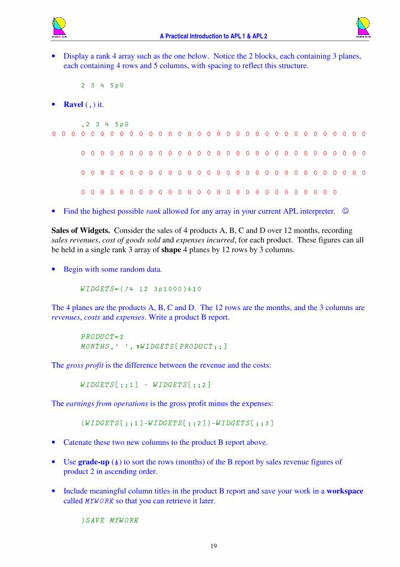
• Display a rank 4 array such as the one below. Notice the 2 blocks, each containing 3 planes,
each containing 4 rows and 5 columns, with spacing to reflect this structure.
2 3 4 5½0
• Ravel (,) it.
,2 3 4 5½0 0 0 0 0 0 0 0 0 0 0 0 0 0 0 0 0 0 0 0 0 0 0 0 0 0 0 0 0 0 0 0 0 0 0 0 0 0 0 0 0 0 0 0 0 0 0 0 0 0 0 0 0 0 0 0 0 0 0 0 0 0 0 0 0 0 0 0 0 0 0 0 0 0 0 0 0 0 0 0 0 0 0 0 0 0 0 0 0 0 0 0 0 0 0 0 0 0 0 0 0 0 0 0 0 0 0 0 0 0 0 0 0 0 0 0 0 0 0 0 0
• Find the highest possible rank allowed for any array in your current APL interpreter. ☺
Sales of Widgets. Consider the sales of 4 products A, B, C and D over 12 months, recording
sales revenues, cost of goods sold and expenses incurred, for each product. These figures can all
be held in a single rank 3 array of shape 4 planes by 12 rows by 3 columns.
• Begin with some random data.
WIDGETS„(?4 12 3½1000)÷10
The 4 planes are the products A, B, C and D. The 12 rows are the months, and the 3 columns are
revenues, costs and expenses. Write a product B report.
PRODUCT„2 MONTHS,' ', •WIDGETS[PRODUCT;;]
The gross profit is the difference between the revenue and the costs:
WIDGETS[;;1] - WIDGETS[;;2]
The earnings from operations is the gross profit minus the expenses:
(WIDGETS[;;1]-WIDGETS[;;2])-WIDGETS[;;3]
• Catenate these two new columns to the product B report above.
• Use grade-up (“) to sort the rows (months) of the B report by sales revenue figures of
product 2 in ascending order.
• Include meaningful column titles in the product B report and save your work in a workspace
called MYWORK so that you can retrieve it later.
)SAVE MYWORK

A Practical Introduction to APL 1 & APL 2
20
L E S S O N 4
APL Programming
A name may be assigned to the result of an expression, and is then called a variable. A name
may be associated with an expression itself, and is then called a user-defined function, or
program, which can be applied to a variety of different arguments. A function executes some
action on its argument(s) to produce a result which may be an argument to a further function.
Here is a very simple example of a user defined function which does nothing more than add its
left argument, which has been named L, to its right argument, which has been named R, and
return the result, which has been named T for total.
’ T„L MYPLUS R [1] T„L+R [2] ’
• To start the editor, type the del symbol (’) followed by the header line followed by Enter.
’ T„L MYPLUS R
This opens the editor and prompts you to type a statement on line 1 by printing the first line
number in brackets followed by some spaces.
[1]
• Type T„L+R and hit Enter. A prompt for the next line is issued.
[2]
Any number of lines can be added to a single function. Execution flows from one line to the
next, consecutively by default. Sometimes functions can have hundreds of lines, sometimes only
one. When all the statements needed to build the result of a function have been entered, the
function definition may be terminated by entering a closing del (’). The user then exits the editor
and returns to immediate execution mode.
[2] ’
Depending upon the particular version of APL being used, the editor may be either the basic line
editor (available in most versions of APL) or a full-screen editor with many built-in WYSIWYG
features. In order to use the APL2 full-screen editor you should execute the system command
)EDITOR 2
A Practical Introduction to APL 1 & APL 2
21
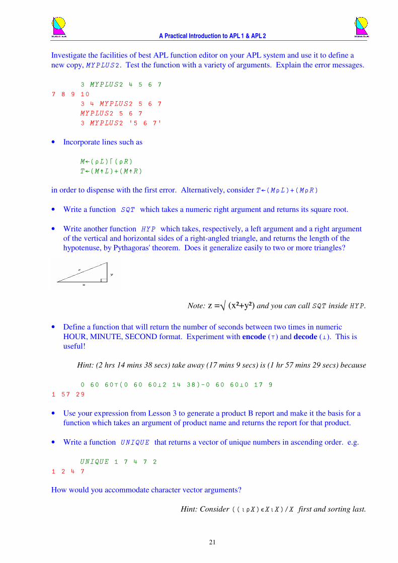
Investigate the facilities of best APL function editor on your APL system and use it to define a
new copy, MYPLUS2. Test the function with a variety of arguments. Explain the error messages.
3 MYPLUS2 4 5 6 7 7 8 9 10 3 4 MYPLUS2 5 6 7 MYPLUS2 5 6 7 3 MYPLUS2 '5 6 7'
• Incorporate lines such as
M„(½L)—(½R) T„(M†L)+(M†R)
in order to dispense with the first error. Alternatively, consider T„(M½L)+(M½R)
• Write a function SQT which takes a numeric right argument and returns its square root.
• Write another function HYP which takes, respectively, a left argument and a right argument
of the vertical and horizontal sides of a right-angled triangle, and returns the length of the
hypotenuse, by Pythagoras' theorem. Does it generalize easily to two or more triangles?
Note: z =√ (x²+y²) and you can call SQT inside HYP.
• Define a function that will return the number of seconds between two times in numeric
HOUR, MINUTE, SECOND format. Experiment with encode (‚) and decode (ƒ). This is
useful!
Hint: (2 hrs 14 mins 38 secs) take away (17 mins 9 secs) is (1 hr 57 mins 29 secs) because
0 60 60‚(0 60 60ƒ2 14 38)-0 60 60ƒ0 17 9 1 57 29
• Use your expression from Lesson 3 to generate a product B report and make it the basis for a
function which takes an argument of product name and returns the report for that product.
• Write a function UNIQUE that returns a vector of unique numbers in ascending order. e.g.
UNIQUE 1 7 4 7 2 1 2 4 7
How would you accommodate character vector arguments?
Hint: Consider ((¼½X)¹X¼X)/X first and sorting last.
A Practical Introduction to APL 1 & APL 2
22
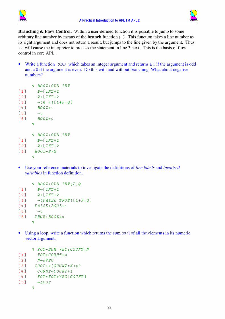
Branching & Flow Control. Within a user-defined function it is possible to jump to some
arbitrary line number by means of the branch function (…). This function takes a line number as
its right argument and does not return a result, but jumps to the line given by the argument. Thus
…3 will cause the interpreter to process the statement in line 3 next. This is the basis of flow
control in core APL.
• Write a function ODD which takes an integer argument and returns a 1 if the argument is odd
and a 0 if the argument is even. Do this with and without branching. What about negative
numbers?
’ BOOL„ODD INT [1] P„—INT÷2 [2] Q„˜INT÷2 [3] …(6 4)[1+P=Q] [4] BOOL„1 [5] …0 [6] BOOL„0 ’
’ BOOL„ODD INT [1] P„—INT÷2 [2] Q„˜INT÷2 [3] BOOL„P¬Q ’
• Use your reference materials to investigate the definitions of line labels and localised
variables in function definition.
’ BOOL„ODD INT;P;Q [1] P„—INT÷2 [2] Q„˜INT÷2 [3] …(FALSE TRUE)[1+P=Q] [4] FALSE:BOOL„1 [5] …0 [6] TRUE:BOOL„0 ’
• Using a loop, write a function which returns the sum total of all the elements in its numeric
vector argument.
’ TOT„SUM VEC;COUNT;N [1] TOT„COUNT„0 [2] N„½VEC [3] LOOP:…(COUNT=N)½0 [4] COUNT„COUNT+1 [4] TOT„TOT+VEC[COUNT] [5] …LOOP ’

A Practical Introduction to APL 1 & APL 2
23
L E S S O N 5
Revising Functions
To change a function which already exists, enter del (’), followed by the name of a function. It is
then presented for editing. (Note that a closing del is required to exit line edit mode.)
’ MYPLUS
• Explore the facilities of your recommended APL function editor. Change the function
MYPLUS, as you feel appropriate, to make a new function MYTIMES.
• Modify the function HYP to take a left argument and a right argument of the (x, y) coordinates
of the start and end of a line, and return the length of the line by Pythagoras' theorem.
z = √ ((x1-x2)² + (y1-y2)²)
• Check that HYP gives the correct result for a 3-4-5 triangle and suggest an alternative syntax.
0 3 HYP ¯4 0
Line 0 Syntax. The header line, or line [0], of a user-defined function specifies the calling
syntax for the function. The structure of this line determines whether the function is dyadic,
monadic or niladic (no arguments). It also determines whether the function returns a result.
Quad Input. Quad (Œ) is a variable which communicates between the user’s terminal and APL.
When Œ is referenced, a prompt (Œ:) is displayed indicating that input is being requested.
• For example, type
X „ Œ Enter this Œ: System prompts with this 3 User types in this X Enter this 3 X has value 3
• Write a niladic function called ASK which does not return a result. This function should ask
the user to type in his gas and electricity meter readings and then ask the user to type in the
cost, in pence, of one unit of gas and electricity. The function should then print out the total
bill rounded to the nearest penny. The session might appear like this:
ASK What are your Gas and Electricity meter readings? Œ: 346 1537 What are your Gas and Electricity unit costs in pence? Œ: 0.132 0.0977 Your total energy bill is £195.84p

A Practical Introduction to APL 1 & APL 2
24
L E S S O N 6
Some Useful System Commands
System commands are all introduced by an ‘unlikely’ first character; right parenthesis. This
would clearly cause an error in any APL expression and therefore causes no conflict or confusion
between calls to the operating system and well formed lines of APL code which may be
incorporated in functions.
• In order to store on file the variables and functions which you have written, type
)SAVE MYWORK
This will save a snapshot of your workspace in a file called MYWORK on disk.
• In order to reinstate this workspace at any time, use the command
)LOAD MYWORK
• Other useful system commands include
)VARS
which lists the global variables that you have assigned, and
)FNS
which lists the functions that you have defined in the current workspace.
Other important system commands include
)SI )RESET )ERASE ... )COPY ... )WSID )CLEAR
and, last but not least, (because you may need it at the end of the day)
)OFF
which terminates the APL session.
A Practical Introduction to APL 1 & APL 2
25
A Practical Introduction to
APL 1&2
...programming, that is, the construction of a desired
function from a set of available primitive functions.
Ken Iverson
Day 2 : Second Generation – APL 2
APL 2 - Nested Arrays Session 3
System Functions & Variables
Primitive Operators
Expressions & Statements
Order of Execution of Operators
Loops v APL (S-Matrix) Thinking
Enclose & Vector Notation Session 4
Each Operator
Binding Strengths
Empty Arrays
Building Tools
Supplied Workspaces
Evolution of APL (1956-2004)
...the ability to translate into APL procedures of interest in your own profession...
Ken Iverson
A Practical Introduction to APL 1 & APL 2
26
L E S S O N 7
Some Useful System Functions
System functions are functions which perform a task outside the domain of the APL workspace.
They can be called within lines of APL code, unlike system commands which can not be called in
an APL program. Some of these system functions perform tasks that were originally only
available through system commands. For example, ŒEX expunges names.
ŒEX 'NUMS'
does the same as
)ERASE NUMS
And
ŒNL 2
returns a character matrix (name list) that includes all global class 2 names which are listed by
)VARS
• Try
ŒNL 2 3
The class of a name (name class) is returned by monadic ŒNC .
A very powerful system function, called ŒFX, fixes a new function defined by its character right
argument.
• Try, for example,
ŒFX 2 9½'R„L IF C R„C/L '
List all the functions in the workspace. Why has this function been called IF?
This system function (ŒFX) is one of the reasons why APL is said to be “self-conscious”, and
cannot, in general, be compiled. The execute function (–) is another metamathematical concept
in the language. You can write programs that write programs whose properties may not be
deducible at the compilation stage.
• Useful niladic system functions include
ŒAI which returns current account information,
ŒTS whose result contains the current system time stamp,
A Practical Introduction to APL 1 & APL 2
27
and
ŒWA which evaluates the remaining workspace available.
A function that has been interrupted is said to be suspended on a certain line. The system
function ŒLC returns the line count, and therefore
…ŒLC
is often used to resume execution from the line at which execution has been halted.
• A favourite system function is (niladic) ŒAV which returns the 256 element atomic vector.
Try it. :-)
• Why is ŒAV a niladic function and not a variable? Why does it have 256 elements?
System Variables. There are also a number of noteworthy system variables. They can be set
(assigned) by the programmer and may have a profound effect on the results of APL expressions.
For example, the primitive function interval (¼) returns an initial ordered subset of the natural
numbers or a subset of the whole numbers depending upon the value of the index origin (ŒIO).
• Type in the following. Observe and explain the differences.
ŒIO„0 ¼9 0 1 2 3 4 5 6 7 8 ?9 5 ŒIO„1 ¼9 1 2 3 4 5 6 7 8 9 ?9 3
• Why does the following give the same answer whatever the index origin.
'abcdefghij'[“”10½1 0] afbgchdiej
• Write a simple APL model of some fuzzy rule-based system, };-)>
basing your model on the conclusions you reach from the results of
1<1.00000000001 1 ŒCT„1E¯10 1<1.00000000001 0
A Practical Introduction to APL 1 & APL 2
28
L E S S O N 8
Primitive APL Operators
"By relieving the brain of all unnecessary work, a good notation sets it free to concentrate on
more advanced problems…," explains A.N.Whitehead. "The quantity of meaning compressed
into a small space by algebraic signs .. facilitates the reasonings we are accustomed to carry on
by their aid," observes Charles Babbage.
The ease of expressing constructs which arise in problems is one objective test that can be applied
to a notation. We saw the difficulty we had in simply adding together all the elements in a vector.
We now introduce the concept of an APL operator that solves this problem in a very powerful
way. "An operator may be applied to a function to derive a different function," says the IBM APL
Language manual of 1978.
General mathematical notation includes Σ to signify the sum of a series and Π to signify the
product of a series. The linear APL notation introduces an operator reduce (/) which applies to a
function, such as plus or times, to produce a derived function, such as sum or product.
+ / 1 2 3 4 5 15
This adds up all the numbers 1 to 5 by conceptually putting a + between all the elements. Thus
+/ can be read as plus reduce and, in this case, is equivalent to
1+2+3+4+5 15
Equally, by this definition of the derived function,
× / 1 2 3 4 5 120
multiplies together all the numbers 1 to 5 by conceptually putting a × between all the elements.
×/ can be read as times reduce and is equivalent to
1×2×3×4×5 120
In other words the mathematical statement ∑=
n
i
iX1
is equivalent to +/X in APL and i
n
i
XΠ=1
is ×/X .
• Sum the squares of the first 10 positive integers.
• Write a function which returns the largest number in a list.
Experiment with reduce operands — ˜ - ÷ ^ Ÿ , giving arguments to the derived functions
that are rank 2, 3 or above. Which dimension is “reduced”? Try to express some algebraic
identities, such as (+/X½Y) − (Y×X) or (×/X½Y) − (Y*X)
A Practical Introduction to APL 1 & APL 2
29
A second operator introduced in core APL is scan (\). Like reduce, this operator applies to all
dyadic scalar functions to produce a derived function that is conceptually similar to placing the
dyadic scalar function between each of the elements along the last axis of the argument.
However, scan generates all the intermediate values as well.
• Notice how
+\1 2 3 4 5 1 3 6 10 15
gives all the (cumulative sum) results
1 1+2 1+2+3 1+2+3+4 1+2+3+4+5
• Explain the result of
-\1 2 3 4 5 1 ¯1 2 ¯2 3
• Check the truth values of
^/(+\X½Y)=(Y×¼X) ^/(×\X½Y)=(Y*¼X)
• Experiment with scan applied to — ˜ - ÷ and especially to ^ Ÿ Š < ˆ ¬
Notice how an operator that takes only one (function or array) operand has it to the left of the
operator symbol, while a function which has only one (array) argument has it placed on the right
of the function symbol. This simple distinction increases the number of parsing rules in the core
APL language from 1 to 2! (The second grammatical rule in APL is a bit like the rule in English
that the subject of a sentence comes before the verb.)
Rule 2: The left function operand of an operator is the function derived from the longest
possible operator sequence to its left.
It is not really possible until lesson 11 to understand the full force of this rule - until operators are
used with derived function arguments. However, it is important to appreciate that these two rules
are ‘essentially’ all that is necessary to specify completely the parsing of any APL 1 statement.
With the above two rules you should be able to read and understand (i.e. interpret) any rational
first generation APL statement. This sentence is circular because by rational we mean any
construct which adheres to rules 1 and 2 only. However, it is still worth saying because one very
respectable goal of APL has been to discard all irrational constructs and replace them with
rational ones. Unfortunately history has tended the other way – to add new arbitrary syntactic
rules to second and third generation APL interpreters.

A Practical Introduction to APL 1 & APL 2
30
• Define a function that returns the average of a vector of numbers when the function argument
is a vector, or the row averages when the argument is a matrix. Discuss how a primitive
operator might be defined that specifies subarrays to which this AVERAGE function applies?
Operators may apply to two operands (c.f. arguments) but, unlike functions, they can NOT be
ambipotent (c.f. ambivalent). An operator, exclusively, either takes one operand on its left or
two operands, one on the left and one on the right (i.e. it is monistic xor dualistic). [Usually the
words monadic, dyadic and valency are applied equally to functions and operators but here I
introduce new words monistic, dualistic and potency to help the (newbie) APLer to clarify the
important distinction between function and operator syntax.]
The inner-product, or the dot operator (.), requires two function arguments that combine in a
given way to produce a dyadic derived function. In the case where the left operand is plus and
the right operand is times, the derived function is that of matrix multiplication (which implicitly
involves multiplication and plus reduction).
• Given some small test matrix,
MAT„3 3½¼4
verify the results of
MAT+.×MAT MAT+.׳MAT MAT^.=³MAT MAT^.=MAT MAT—.+MAT
• In what context might each of the above derived functions be used? Consider, for example a
statement such as
TOTAL_COST „ COSTS +.× QUANTITIES
In the early days of APL 1, operators were not well understood and a couple of syntactically
irrational operator constructs were introduced. (See e.g. Rationalised APL by K.E.Iverson,
1981.) For example, the two symbols jot (°) and dot are used in combination to represent the
outer- product operator. This operator derives a dyadic function which conceptually takes each
element of its left argument and combines it with each and every element in the right argument
according to the dyadic (right) operand.
• Enter these two examples and find an example of another useful operand.
(¼7) °.+ (¼7) © addition table 2 3 4 5 6 7 8 3 4 5 6 7 8 9 4 5 6 7 8 9 10 5 6 7 8 9 10 11 6 7 8 9 10 11 12 7 8 9 10 11 12 13 8 9 10 11 12 13 14

A Practical Introduction to APL 1 & APL 2
31
(¼7) °.× (¼7) © multiplication table 1 2 3 4 5 6 7 2 4 6 8 10 12 14 3 6 9 12 15 18 21 4 8 12 16 20 24 28 5 10 15 20 25 30 35 6 12 18 24 30 36 42 7 14 21 28 35 42 49
Notice the appearance of the comment symbol (©) which can be used to add comments at the end
of any executable line of APL.
Aside: The jot-dot-times derived function, although irrational in its syntax, has been so admired
by APLers that an American APL journal was named after it. There is also an American journal
called APL Quote-Quad. Quote-quad is an I/O variable like quad (Œ) but for characters. It is
written x. Likewise there was an APL company called Inner Product and another called Dyadic
Systems. Dyadic Systems had an Outer Products catalogue of end user solutions. Puns or
what?! It is of interest to note that the name Dyalog originates from a joint project between
Dyadic and Zilog whose outcome was the first version of the Dyalog APL interpreter in 1982:-)
The axis operator has irregular syntax. It surrounds its numeric “right” operand with brackets.
This, like indexing, does not follow the usual single token nomenclature which is assumed in
rules 1 and 2. (But IBM APL2 and Dyalog now have a rational dyadic index function (¦).)
• Experiment with
²[ŒIO]MAT 3 4 1 4 1 2 1 2 3 ²[1+ŒIO]MAT 3 2 1 2 1 4 1 4 3 and
MAT,[ŒIO]MAT 1 2 3 4 1 2 3 4 1 1 2 3 4 1 2 3 4 1 MAT,[1+ŒIO]MAT 1 2 3 1 2 3 4 1 2 4 1 2 3 4 1 3 4 1
to see how the axis operator modifies the axis to which its left operand applies.

A Practical Introduction to APL 1 & APL 2
32
In the penultimate example above, the catenate function (,) becomes the derived function
catenate-along-first-axis (,[1]) which can also be programmed as catenate-first (®) .
• Hence check the meaning of
+/[1]MAT 8 7 6 and
+/[2]MAT 6 7 8 • What might the following line of code be doing?
((+/[2]EXPENSES_BY_MONTH)>2500)/[1]SALESMEN
• Can you identify any other irrational syntax (i.e. irregular use of tokens vis-à-vis rules 1 and
2) in any of the preceding lessons? Is / a function or an operator?
Remember, you're not really supposed to encounter anything irrational in APL notation!
Grammar: Core APL, here called APL 1, has an extremely simple and elegant grammar. This
grammar still forms the unchanged core of modern APLs, which adhere quite strictly to ISO
Standard 8485:1989. Later generations, APL 2 and APL 3, each introduce a number of new rules
of grammar making the underlying parsers considerably more complicated, and consequently,
lines of code harder to read with confidence. Nevertheless, the original two grammatical rules of
APL 1 still hold good and form a solid, clear foundation for the whole language. Fluency in APL
follows from a secure understanding of the two fundamental rules of grammar stated in Lessons 1
and 8.
A Practical Introduction to APL 1 & APL 2
33
L E S S O N 9
APL Thinking
Most 20th
century computer languages have evolved from representations of sequential
instructions in digital memory. APL syntax, on the other hand, evolved from traditional
mathematical notation. This explains the relative ease with which complex ideas can be
translated into APL programs. As a result APL has been, and still remains, irreplaceable for
many diverse mission-critical systems found in large organisations all over the world.
• Insert lots of redundant parentheses to show the steps involved in this statement:
SCALE „ 4 5 6 + 3 × ¼ 9 - 6
• Construct the following matrix in the clearest possible way, and then again using as few
syntactic elements (tokens) as possible:
0 3 2 1
1 0 3 2
2 1 0 3
• Define a function which will remove any of a list of unwanted characters (the left argument)
from a matrix (the right argument) and replace them with spaces. This is not a common
utility but you’ve got to feel confident that you can quickly produce it if you need it. If it is
destined to become a common utility then you should make sure that it is suitably general; it
applies to all appropriate ranks of array arguments including zero rank and other empty
arrays, it applies to numbers too, perhaps it even signals its own specific errors and it can
never halt in the middle. In other words, it should be modelled on the design of primitive APL
functions such as member (¹).
If you think that is too easy then show, instead, how to construct some interesting looking matrix
with just a few tokens. If you think that is too simple as well, then generate all the whole
numbers from 1 to 100 using any APL primitives but only using the digits 1,9,8 and 6 once each
and in that order. Thus, for example, the number 1 is given by
1˜986 1
and the number 42 is given by
19——8*µ6 42
An amazing complete answer to this wonderful challenge is to be found in the fascinating and
useful Journal of the British APL Association, in Vector Vol.3 No.2 p105 (1986).
A Practical Introduction to APL 1 & APL 2
34
Scalars & Loops versus Vector Operations. We have seen how it is possible to write a looping
function that will add up all the elements in a vector. This should be replaced by the derived
function plus reduce (or sum) for reasons of both elegance and efficiency. Plus reduce also
extends naturally to sum over the rows, or sum over the planes by way of the axis operator (or by
dyadic transpose (³), or by reduce-first (š) ...).
In APL one attempts to apply some function to the given arguments to obtain immediately the
desired result. This is not always possible; often intermediate results are needed. If so, the
problem is broken down into sub-problems and a solution to each sub-problem is then sought
through the application of some function to an argument or arguments to give an intermediate
result. It is amazing how seldom (if ever) loops are strictly necessary, even in core APL 1. (In
APL 2, as we shall see, loops are employed even less often.)
Aside:
This black-box, operational way of thinking [input/operation/output] is reminiscent of the scattering-
matrix approach to quantum mechanics which was popular amongst particle physicists in the 1970’s (see
The Tao of Physics by Fritjov Capra). One can observe what (particle) goes in and what (particle) comes
out, but one can never see what “actually happens” inside a sufficiently small black circle.
Mathematically, the (possibly infinite) matrix operation S simply transforms the (Hilbert space) vector IN
to vector OUT. Bootstrap philosophy attempted to specify the S-matrix elements entirely through self-
consistency with related S-matrices but then quantum chromo-dynamics (QCD) was discovered (c. 1973)
which seems to describe accurately the behaviour of quarks and so theoretical physicists moved back to
field theory thinking.
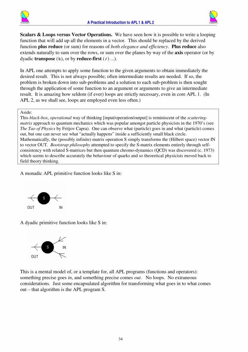
A monadic APL primitive function looks like S in:
A dyadic primitive function looks like S in:
This is a mental model of, or a template for, all APL programs (functions and operators):
something precise goes in, and something precise comes out. No loops. No extraneous
considerations. Just some encapsulated algorithm for transforming what goes in to what comes
out – that algorithm is the APL program S.
A Practical Introduction to APL 1 & APL 2
35
Sometimes apparently unavoidable loops can be avoided by recursion. The Fibonacci series is
elegantly generated through a recursive function. Each term in the series is the sum of the
preceding two terms, starting with 1 1. The function below takes a whole number, N, and returns
the first N Fibonacci numbers.
’ Z„FIBONACCI N [1] © Z is the first N terms of the Fibonacci series [2] –(N=1)/'…~Z„1' [3] Z„Z,+/¯2†Z„FIBONACCI N-1 ’ • Study this function. Predict what will happen if N is zero. Verify that the quotient of the last
2 numbers of a finite Fibonacci series tends to the Golden Mean ((5*0.5)-1)÷2
Hint: Remember Ctrl+C on a mainframe or Ctrl+Break on a PC!
Aside:
The Golden Mean is believed by some to control psychology in the city? It appears that when a market
price is ready for a big change, the next stable point downwards is the product with the Golden Mean, and
the next stable point upwards is the quotient!
• Define a recursive FACTORIAL function which takes a whole number argument, N, and
returns the factorial (!) of N, i.e. N×(N-1)×(N-2)×..×2×1 .
Hint: If N is not zero, then the result is N×FACTORIAL(N-1).
• The following function converts a date to an International Day Number. Is the function
IDN_FROM_TS millennium-proof? :-S
’ IDN„IDN_FROM_TS TS;YY;MM;DD;LP;DDM [1] © Convert date from 3-element vector (3†ŒTS) to IDN [2] –(0=+/TS)/'…IDN„0' [3] YY MM DD„TS © Split args. [4] LP„-/0=400 100 4|YY © Leap year ***** [5] DDM„0 31,LP+59 90 120 151 181 212 243 273 304 334 [6] IDN„˜365.25×YY-1900 © Convert years. [7] IDN„IDN+1†MM‡0,DDM © .. months. [8] IDN„IDN+DD-LP © .. days. [9] IDN„IDN+IDN<0 © Days before 1900-01-01 are ˆ 0. ’
• Discuss the steps involved in programming the inverse function TS_FROM_IDN. �
A Practical Introduction to APL 1 & APL 2
36
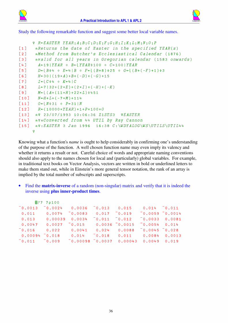
Study the following remarkable function and suggest some better local variable names.
’ R„EASTER YEAR;A;B;C;D;E;F;G;H;I;K;L;M;N;O;P [1] ©Returns the date of Easter in the specified YEAR(s) [2] ©Method from Butcher's Ecclesiastical Calendar (1876) [3] ©valid for all years in Gregorian calendar (1583 onwards) [4] A„19|YEAR ª B„˜YEAR÷100 ª C„100|YEAR [5] D„˜B÷4 ª E„4|B ª F„˜(B+8)÷25 ª G„˜(B+(-F)+1)÷3 [6] H„30|(19×A)+B+(-D)+(-G)+15 [7] I„˜C÷4 ª K„4|C [8] L„7|32+(2×E)+(2×I)+(-H)+(-K) [9] M„˜(A+(11×H)+22×L)÷451 [10] N„H+L+(-7×M)+114 [11] O„˜N÷31 ª P„31|N [12] R„(10000×YEAR)+1+P+100×O [13] ©’ 23/07/1993 10:06:36 Z1STS3 ’EASTER [14] ©’©Converted from 44 UTIL by Ray Cannon [15] ©’:EASTER 3 Jan 1996 16:38 C:\WDYALOG\WS\UTILS\UTIL44 ’
Knowing what a function's name is ought to help considerably in confirming one’s understanding
of the purpose of the function. A well chosen function name may even imply its valency and
whether it returns a result or not. Careful choice of words and appropriate naming conventions
should also apply to the names chosen for local and (particularly) global variables. For example,
in traditional text books on Vector Analysis, vectors are written in bold or underlined letters to
make them stand out, while in Einstein’s more general tensor notation, the rank of an array is
implied by the total number of subscripts and superscripts.
• Find the matrix-inverse of a random (non-singular) matrix and verify that it is indeed the
inverse using plus inner-product times.
�?7 7½100 ¯0.0013 ¯0.0024 0.0036 ¯0.013 0.015 0.014 ¯0.011 0.011 0.0074 ¯0.0083 0.017 ¯0.019 ¯0.0059 ¯0.0014 0.013 0.00039 0.0034 ¯0.011 ¯0.012 ¯0.0033 0.0081 0.0047 0.0027 ¯0.015 0.0036 ¯0.0015 ¯0.0054 0.014 ¯0.016 0.022 0.0041 0.024 0.0088 ¯0.0045 ¯0.028 0.00094 ¯0.018 0.014 ¯0.018 0.011 0.0084 0.0013 ¯0.011 ¯0.009 ¯0.00098 ¯0.0037 0.00043 0.0049 0.019
A Practical Introduction to APL 1 & APL 2
37
L E S S O N 10
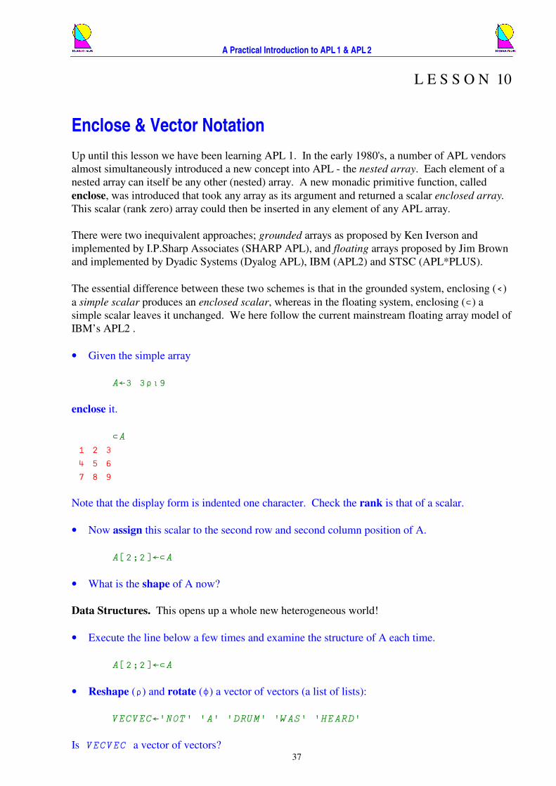
Enclose & Vector Notation
Up until this lesson we have been learning APL 1. In the early 1980's, a number of APL vendors
almost simultaneously introduced a new concept into APL - the nested array. Each element of a
nested array can itself be any other (nested) array. A new monadic primitive function, called
enclose, was introduced that took any array as its argument and returned a scalar enclosed array.
This scalar (rank zero) array could then be inserted in any element of any APL array.
There were two inequivalent approaches; grounded arrays as proposed by Ken Iverson and
implemented by I.P.Sharp Associates (SHARP APL), and floating arrays proposed by Jim Brown
and implemented by Dyadic Systems (Dyalog APL), IBM (APL2) and STSC (APL*PLUS).
The essential difference between these two schemes is that in the grounded system, enclosing (<)
a simple scalar produces an enclosed scalar, whereas in the floating system, enclosing (›) a
simple scalar leaves it unchanged. We here follow the current mainstream floating array model of
IBM’s APL2 .
• Given the simple array
A„3 3½¼9
enclose it.
›A 1 2 3 4 5 6 7 8 9
Note that the display form is indented one character. Check the rank is that of a scalar.
• Now assign this scalar to the second row and second column position of A.
A[2;2]„›A
• What is the shape of A now?
Data Structures. This opens up a whole new heterogeneous world!
• Execute the line below a few times and examine the structure of A each time.
A[2;2]„›A
• Reshape (½) and rotate (²) a vector of vectors (a list of lists):
VECVEC„'NOT' 'A' 'DRUM' 'WAS' 'HEARD'
Is VECVEC a vector of vectors?
A Practical Introduction to APL 1 & APL 2
38
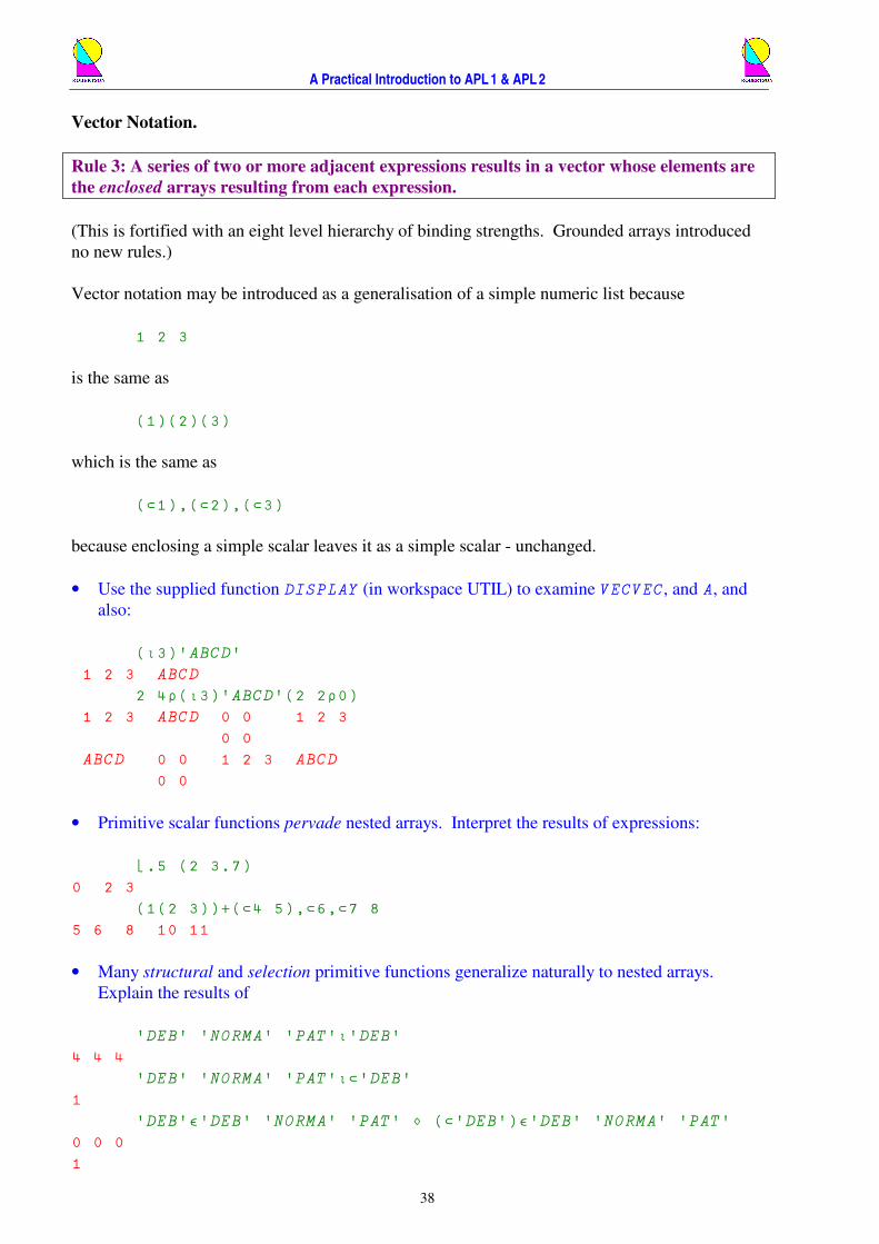
Vector Notation.
Rule 3: A series of two or more adjacent expressions results in a vector whose elements are
the enclosed arrays resulting from each expression.
(This is fortified with an eight level hierarchy of binding strengths. Grounded arrays introduced
no new rules.)
Vector notation may be introduced as a generalisation of a simple numeric list because
1 2 3
is the same as
(1)(2)(3)
which is the same as
(›1),(›2),(›3)
because enclosing a simple scalar leaves it as a simple scalar - unchanged.
• Use the supplied function DISPLAY (in workspace UTIL) to examine VECVEC, and A, and
also:
(¼3)'ABCD' 1 2 3 ABCD 2 4½(¼3)'ABCD'(2 2½0) 1 2 3 ABCD 0 0 1 2 3 0 0 ABCD 0 0 1 2 3 ABCD 0 0
• Primitive scalar functions pervade nested arrays. Interpret the results of expressions:
˜.5 (2 3.7) 0 2 3 (1(2 3))+(›4 5),›6,›7 8 5 6 8 10 11
• Many structural and selection primitive functions generalize naturally to nested arrays.
Explain the results of
'DEB' 'NORMA' 'PAT'¼'DEB' 4 4 4 'DEB' 'NORMA' 'PAT'¼›'DEB' 1 'DEB'¹'DEB' 'NORMA' 'PAT' ª (›'DEB')¹'DEB' 'NORMA' 'PAT' 0 0 0 1

A Practical Introduction to APL 1 & APL 2
39
and give the dyadic epsilon function (¹) a suitable name, after having determined its part of
speech given the grammatical context. ☺
Some new APL 2 primitive functions, for example monadic disclose (œ), monadic first (†) and
dyadic match (−), apply to nested arrays to give well defined results. IBM APL2 (and second
generation SHARP APL) introduced complex numbers as an integral part of the language.
• Experiment with 0J1, which means √-1, and 4J3 which means (4+3i).
¯1*0.5 0J1 4+3×0J1 4J3 +4J3 4J¯3
• Check the result of the complex addition and multiplication.
2.1J3.4 1.4J6.2 + 4J3 6.1J6.4 5.4J9.2 2.1J3.4 1.4J6.2 × 4J3 ¯1.8J19.9 ¯13J29
• Explain the result of µ¯1 by way of the most beautiful and astonishing identity in
mathematics:
1−=πie
A Practical Introduction to APL 1 & APL 2
40
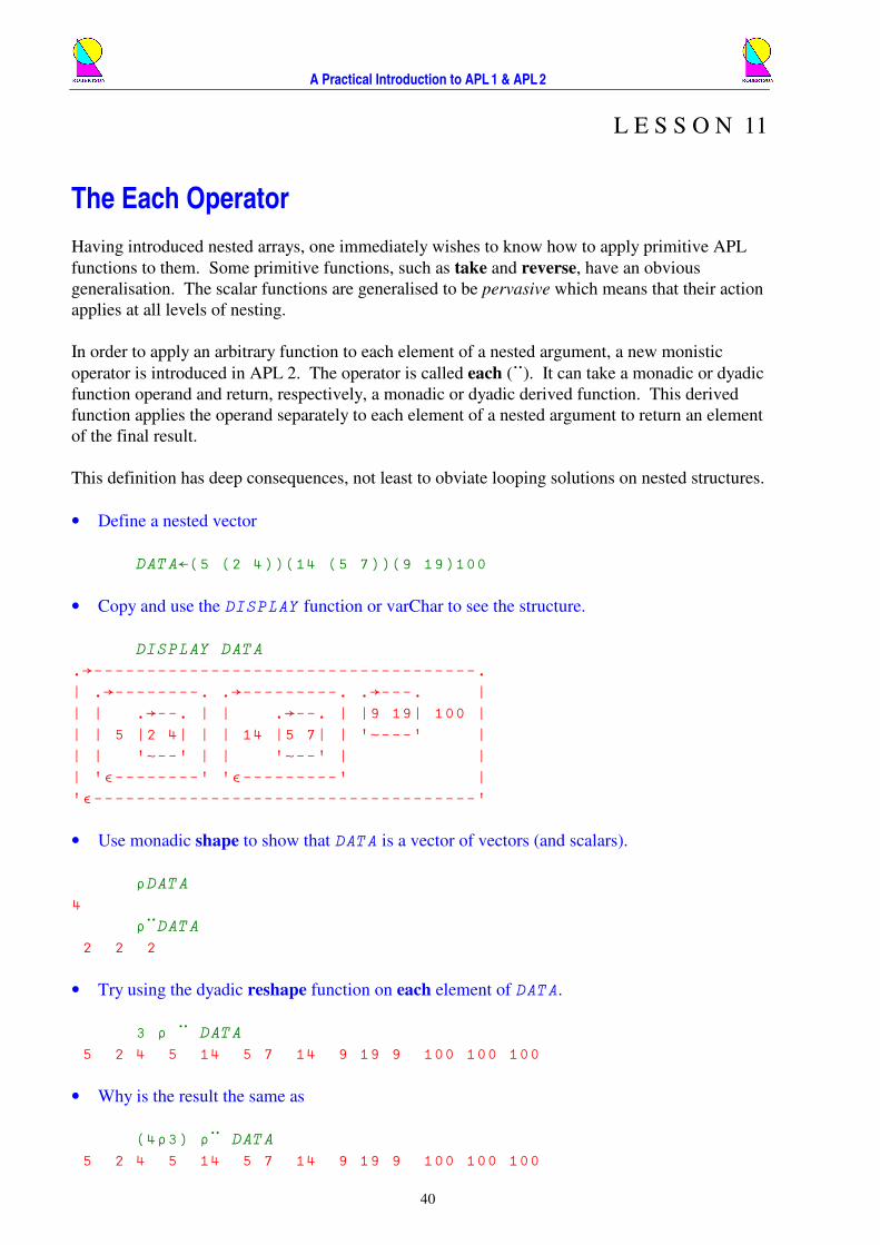
L E S S O N 11
The Each Operator
Having introduced nested arrays, one immediately wishes to know how to apply primitive APL
functions to them. Some primitive functions, such as take and reverse, have an obvious
generalisation. The scalar functions are generalised to be pervasive which means that their action
applies at all levels of nesting.
In order to apply an arbitrary function to each element of a nested argument, a new monistic
operator is introduced in APL 2. The operator is called each (¨). It can take a monadic or dyadic
function operand and return, respectively, a monadic or dyadic derived function. This derived
function applies the operand separately to each element of a nested argument to return an element
of the final result.
This definition has deep consequences, not least to obviate looping solutions on nested structures.
• Define a nested vector
DATA„(5 (2 4))(14 (5 7))(9 19)100
• Copy and use the DISPLAY function or varChar to see the structure.
DISPLAY DATA .…------------------------------------. | .…--------. .…---------. .…---. | | | .…--. | | .…--. | |9 19| 100 | | | 5 |2 4| | | 14 |5 7| | '~---' | | | '~--' | | '~--' | | | '¹--------' '¹---------' | '¹------------------------------------'
• Use monadic shape to show that DATA is a vector of vectors (and scalars).
½DATA 4 ½¨DATA 2 2 2
• Try using the dyadic reshape function on each element of DATA.
3 ½ ¨ DATA 5 2 4 5 14 5 7 14 9 19 9 100 100 100
• Why is the result the same as
(4½3) ½¨ DATA 5 2 4 5 14 5 7 14 9 19 9 100 100 100

A Practical Introduction to APL 1 & APL 2
41
• How many lines of code are there in all the functions in your workspace?
Hint: Consider the shape of each of ŒCR¨›[2]ŒNL 3 • Notice and understand the differences between
²DATA 100 9 19 14 5 7 5 2 4
and
²¨DATA 2 4 5 5 7 14 19 9 100 and
²¨¨DATA 5 4 2 14 7 5 9 19 100
• What will be the results of
4 5 3 4†¨DATA
and
1 2 1 1‡¨DATA
Hint: What is the shape of 1‡0 or 1‡'A' ? Ouch! Oooo! :-O
In APL, scalars are rank zero arrays and as such they fit very neatly into the whole APL data
scheme. Thus the shape of a numeric scalar is a vector of length zero, such as 0½0. The shape of
a vector (rank one) is a vector of length one, such as ,5 . The shape of a matrix (rank two) is a
vector of length two, such as 10 10 . The shape of a rank three array is a vector of length
three, such as 3 4 5. etc…
• Predict the result of, and simplify, expression
2½(0½0)½0 • Investigate the results of
3½¨(¼8)2(²¼6) 1 2 3 2 2 2 6 5 4 3œ¨(¼8)(¼7)(²¼6) 3 3 4 2†¨,¨(2 2½5)(3 3½6) 5 5 6 6 ½¨¨¨›(2 3)(2 2½¼4)(›3½4) 3
A Practical Introduction to APL 1 & APL 2
42
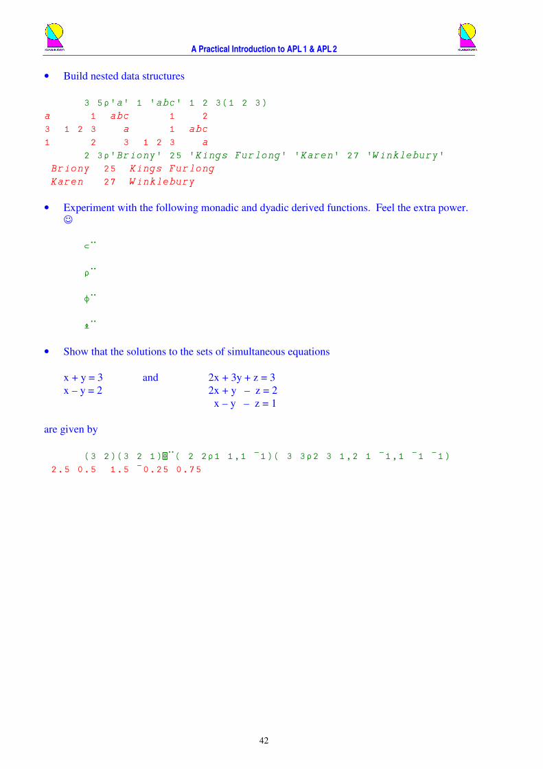
• Build nested data structures
3 5½'a' 1 'abc' 1 2 3(1 2 3) a 1 abc 1 2 3 1 2 3 a 1 abc 1 2 3 1 2 3 a 2 3½'Briony' 25 'Kings Furlong' 'Karen' 27 'Winklebury' Briony 25 Kings Furlong Karen 27 Winklebury
• Experiment with the following monadic and dyadic derived functions. Feel the extra power. ☺
›¨ ½¨ ²¨ –¨ • Show that the solutions to the sets of simultaneous equations
x + y = 3 and 2x + 3y + z = 3
x – y = 2 2x + y – z = 2
x – y – z = 1
are given by
(3 2)(3 2 1)�¨( 2 2½1 1,1 ¯1)( 3 3½2 3 1,2 1 ¯1,1 ¯1 ¯1) 2.5 0.5 1.5 ¯0.25 0.75
A Practical Introduction to APL 1 & APL 2
43
L E S S O N 12
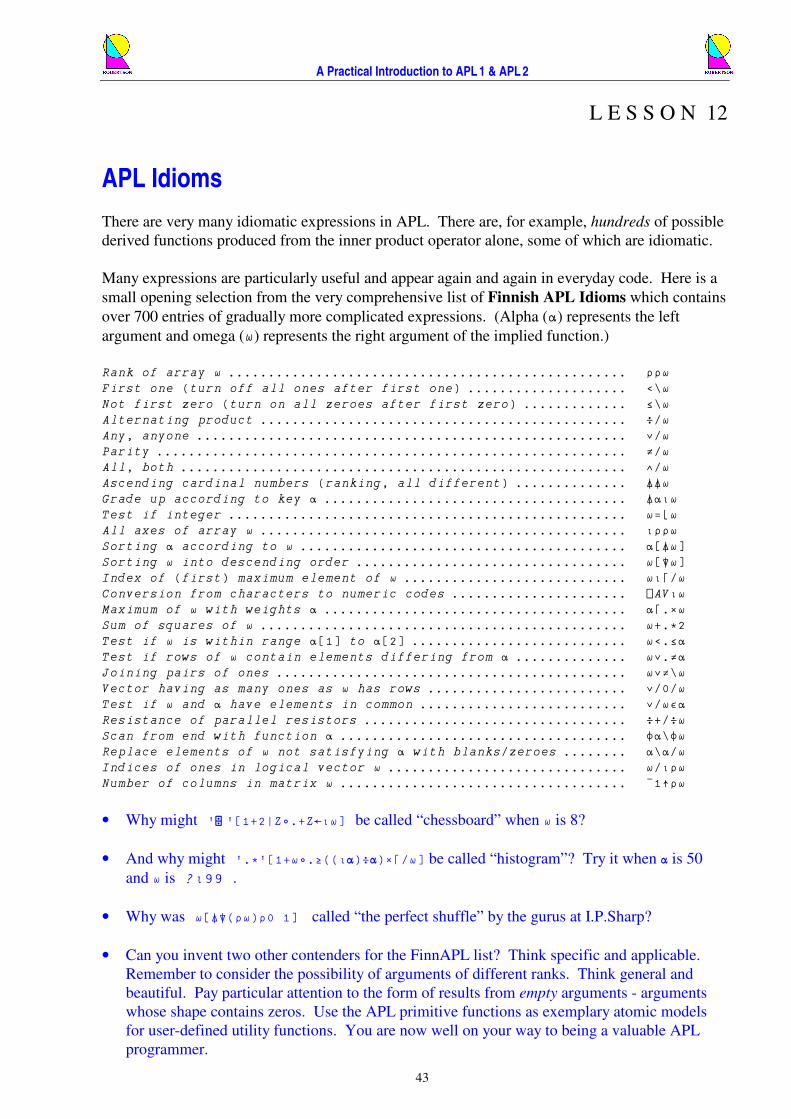
APL Idioms
There are very many idiomatic expressions in APL. There are, for example, hundreds of possible
derived functions produced from the inner product operator alone, some of which are idiomatic.
Many expressions are particularly useful and appear again and again in everyday code. Here is a
small opening selection from the very comprehensive list of Finnish APL Idioms which contains
over 700 entries of gradually more complicated expressions. (Alpha (¸) represents the left
argument and omega (¾) represents the right argument of the implied function.)
Rank of array ¾ .................................................. ½½¾ First one (turn off all ones after first one) .................... <\¾ Not first zero (turn on all zeroes after first zero) ............. ˆ\¾ Alternating product .............................................. ÷/¾ Any, anyone ...................................................... Ÿ/¾ Parity ........................................................... ¬/¾ All, both ........................................................ ^/¾ Ascending cardinal numbers (ranking, all different) .............. ““¾ Grade up according to key ¸ ...................................... “¸¼¾ Test if integer .................................................. ¾=˜¾ All axes of array ¾ .............................................. ¼½½¾ Sorting ¸ according to ¾ ......................................... ¸[“¾] Sorting ¾ into descending order .................................. ¾[”¾] Index of (first) maximum element of ¾ ............................ ¾¼—/¾ Conversion from characters to numeric codes ...................... ŒAV¼¾ Maximum of ¾ with weights ¸ ...................................... ¸—.×¾ Sum of squares of ¾ .............................................. ¾+.*2 Test if ¾ is within range ¸[1] to ¸[2] ........................... ¾<.ˆ¸ Test if rows of ¾ contain elements differing from ¸ .............. ¾Ÿ.¬¸ Joining pairs of ones ............................................ ¾Ÿ¬\¾ Vector having as many ones as ¾ has rows ......................... Ÿ/0/¾ Test if ¾ and ¸ have elements in common .......................... Ÿ/¾¹¸ Resistance of parallel resistors ................................. ÷+/÷¾ Scan from end with function ¸ .................................... ²¸\²¾ Replace elements of ¾ not satisfying ¸ with blanks/zeroes ........ ¸\¸/¾ Indices of ones in logical vector ¾ .............................. ¾/¼½¾ Number of columns in matrix ¾ .................................... ¯1†½¾
• Why might '� '[1+2|Z°.+Z„¼¾] be called “chessboard” when ¾ is 8?
• And why might '.*'[1+¾°.‰((¼Α)÷Α)×—/¾] be called “histogram”? Try it when Α is 50
and ¾ is ?¼99 .
• Why was ¾[“”(½¾)½0 1] called “the perfect shuffle” by the gurus at I.P.Sharp?
• Can you invent two other contenders for the FinnAPL list? Think specific and applicable.
Remember to consider the possibility of arguments of different ranks. Think general and
beautiful. Pay particular attention to the form of results from empty arguments - arguments
whose shape contains zeros. Use the APL primitive functions as exemplary atomic models
for user-defined utility functions. You are now well on your way to being a valuable APL
programmer.

A Practical Introduction to APL 1 & APL 2
44
L E S S O N 13
Building Tools
Good advice to the APLer is Build Tools.
Gather together, or build from scratch, a set of utility functions which are modelled on the APL
primitive functions. Let them do one specific job with argument arrays of any suitable rank and
type. Make sure they have no external impact apart from the results they return (e.g. no change
to global or system variables). These utilities, if well chosen, can form the basic capsules for each
and every new application which you write.
The utility below right justifies a numeric or character vector.
’ VEC„RJUST VEC [1] VEC„(-+/^\²VEC=1†0½VEC)²VEC ’
• Write a function LJUST which left justifies all the rows in a matrix.
Hint: Do this in two distinct steps.
• Write a function which trims the leading (and trailing) spaces from a character vector. This
function is very useful. What might you consider when choosing an appropriate function
name?
• Write a function UCASE which efficiently converts nested character arrays to upper case
letters.
• Write a function, AFTER, which returns a boolean scalar signifying whether or not the left
argument (date) is temporaneously after the right argument (date). :)
• Write scalar dyadic functions, LCM and HCF, which return the lowest common multiple - the
smallest number which is exactly divisible by each of two numbers - and the highest common
factor (or greatest common divisor) - the largest number which divides each exactly.
• When writing an APL function, which of the following suggestions should you adopt?
1) Choose meaningful names in the application context, not single letters.
2) Make functions as short as possible – less than 15 lines long and less than 60 characters per
line.
3) Make programs as fast as possible to run rather than as easy as possible to read.
4) If you can’t avoid global variables, use distinct names; for example, ÇÁÝÁ rather than DATA.
5) Use line labels like Step2: rather than L2: and never branch to absolute line numbers.
6) Don’t put more than one assignment arrow in a statement and avoid loops.
7) Explain the arguments, purpose and result of all functions in a comment at the beginning.
8) APL standards are a matter of individual taste and style and should not be imposed.
• Discuss the APL programming standards which you intend to follow.

A Practical Introduction to APL 1 & APL 2
45
L E S S O N 14
Investigating Supplied Workspaces
Every APL interpreter comes with a treasure trove of supplied workspaces. Some are collections
of utilities, some are small example applications and some are full-blown applications.
• Enter the system command (possibly followed a library name or number)
)LIB
to see the list of workspaces available in your own library, or in a public library.
Warning: Before loading any new workspace, )SAVE your work.
• Find a workspace which sounds interesting and type )LOAD followed by the name of the
workspace (possibly preceded by a library number or directory path).
When you load a workspace the contents of the system variable ŒLX is executed. Thus loading a
workspace may start a whole application.
• If you have started an application, hit the interrupt key (perhaps a second or third time -
sometimes also hit the enter key a couple of times!) to break the execution. (PCs are
somewhat more predictable than mainframes in this regard.) When the program has stopped,
type
)VARS
)FNS
)SI
The State Indicator resulting from the )SI command when a function is suspended shows the
calling structure and the line on which execution halted.
• Use your editor to open the function at the top of the stack, and identify the line on which
execution is suspended.
• A line is restartable if it can be run again and again without changing the outcome. Look
carefully at the suspended line to determine if the line is restartable. If so, type
…ŒLC
otherwise try to restart from an earlier (…ŒLC-1) or later (…ŒLC+1) line or load another
workspace.
Finally, to exit APL, type
)OFF
A Practical Introduction to APL 1 & APL 2
46
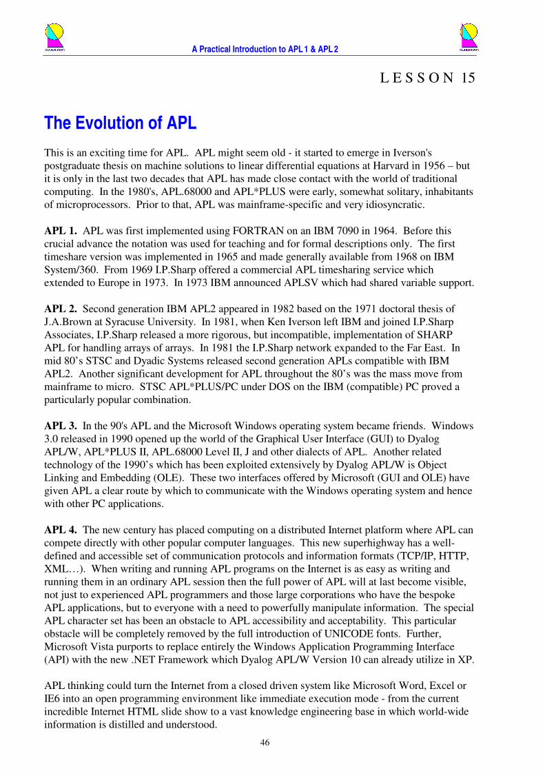
L E S S O N 15
The Evolution of APL
This is an exciting time for APL. APL might seem old - it started to emerge in Iverson's
postgraduate thesis on machine solutions to linear differential equations at Harvard in 1956 – but
it is only in the last two decades that APL has made close contact with the world of traditional
computing. In the 1980's, APL.68000 and APL*PLUS were early, somewhat solitary, inhabitants
of microprocessors. Prior to that, APL was mainframe-specific and very idiosyncratic.
APL 1. APL was first implemented using FORTRAN on an IBM 7090 in 1964. Before this
crucial advance the notation was used for teaching and for formal descriptions only. The first
timeshare version was implemented in 1965 and made generally available from 1968 on IBM
System/360. From 1969 I.P.Sharp offered a commercial APL timesharing service which
extended to Europe in 1973. In 1973 IBM announced APLSV which had shared variable support.
APL 2. Second generation IBM APL2 appeared in 1982 based on the 1971 doctoral thesis of
J.A.Brown at Syracuse University. In 1981, when Ken Iverson left IBM and joined I.P.Sharp
Associates, I.P.Sharp released a more rigorous, but incompatible, implementation of SHARP
APL for handling arrays of arrays. In 1981 the I.P.Sharp network expanded to the Far East. In
mid 80’s STSC and Dyadic Systems released second generation APLs compatible with IBM
APL2. Another significant development for APL throughout the 80’s was the mass move from
mainframe to micro. STSC APL*PLUS/PC under DOS on the IBM (compatible) PC proved a
particularly popular combination.
APL 3. In the 90's APL and the Microsoft Windows operating system became friends. Windows
3.0 released in 1990 opened up the world of the Graphical User Interface (GUI) to Dyalog
APL/W, APL*PLUS II, APL.68000 Level II, J and other dialects of APL. Another related
technology of the 1990’s which has been exploited extensively by Dyalog APL/W is Object
Linking and Embedding (OLE). These two interfaces offered by Microsoft (GUI and OLE) have
given APL a clear route by which to communicate with the Windows operating system and hence
with other PC applications.
APL 4. The new century has placed computing on a distributed Internet platform where APL can
compete directly with other popular computer languages. This new superhighway has a well-
defined and accessible set of communication protocols and information formats (TCP/IP, HTTP,
XML…). When writing and running APL programs on the Internet is as easy as writing and
running them in an ordinary APL session then the full power of APL will at last become visible,
not just to experienced APL programmers and those large corporations who have the bespoke
APL applications, but to everyone with a need to powerfully manipulate information. The special
APL character set has been an obstacle to APL accessibility and acceptability. This particular
obstacle will be completely removed by the full introduction of UNICODE fonts. Further,
Microsoft Vista purports to replace entirely the Windows Application Programming Interface
(API) with the new .NET Framework which Dyalog APL/W Version 10 can already utilize in XP.
APL thinking could turn the Internet from a closed driven system like Microsoft Word, Excel or
IE6 into an open programming environment like immediate execution mode - from the current
incredible Internet HTML slide show to a vast knowledge engineering base in which world-wide
information is distilled and understood.
A Practical Introduction to APL 1 & APL 2
47
One of many examples of the powerful inroads that APL is making onto the new information
superhighway is found in an article by Jonathan Barman in the journal of the British APL
Association. This article describes a utility function which translates an arbitrary APL array into
an XML character string. XML (as well as UNICODE no doubt) has been called "the ASCII of
the future".
XML „ Encode Array
See: J.Barman in Vector Vol 17.4, April 2001, page 48.
• Begin work on a simple application of APL in a topic in your own discipline.
• Go and solve real problems…
• Consider attending further courses on different aspects of APL, such as:
A Practical Introduction to
APL 3&4
with Dyalog APL
Day 1: Third Generation – APL 3 – GUI & OLE
Using GUI Objects (ŒWC)
Object Properties & Methods
Object Events & Callback Functions (ŒDQ)
Looking inside the APL Session (ŒSE)
Understanding Dot Syntax
Arrays of Namespaces
Getting into Word & Excel from APL (OLE)
Writing In-Process OLE Servers (.DLL)
Writing ActiveX Controls (.OCX)
How to Access Functions in .DLLs (ŒNA)
Control Structures
Making Runtime .EXEs
Day 2: Fourth Generation – APL 4 – TCP/IP & .NET
Dynamic Functions & Operators
Introduction to MultiThreading
Aspects of Pocket APL
Understanding TCP/IP Sockets
Browsing the Internet from APL
Hosting an APL Web Server
Introduction to Dyalog .NET
Writing .NET Classes
Writing Web Services
Writing ASP.NET Web Pages
Writing Dyalog APL Classes
A Practical Introduction to APL 1 & APL 2
48
F U R T H E R R E S E A R C H
This 2-day course is just an introduction to the big, wide world of APL programming. For current
information on APL you should subscribe to Vector magazine (the Journal of the British APL
Association), and visit the Vector web site at
http://www.vector.org.uk/
Or subscribe to APL Quote Quad and visit the American special interest group web site at
http://www.acm.org/sigapl/
Many other APL organizations and links may be found in, for example,
http://www.acm.org/sigs/sigapl/orgs.htm
or
http://www.rexswain.com/aplinfo.html
or
http://www.chilton.com/~jimw/others.html
or
http://www.lescasse.com/TSPX5.asp
For an example of a modern successful APL application, see
http://www.grapl.com/
There is also a steady stream of miscellaneous opinions, questions and answers about APL in the
open Google comp.lang.apl group to be found at
http://groups.google.com/groups?hl=en&lr=&ie=UTF-8&group=comp.lang.apl
* * * * *
A Practical Introduction to APL 1 & APL 2
49
F E E D B A C K F O R M
Date _____________________ Instructor _____________________
Name _____________________ Course Name _____________________
eMail _____________________ Location _____________________
Please indicate your view of the following:
poor 1 2 3 4 5 excellent
Location & Facilities
Course Content
Course Material
Instructor’s Knowledge
How useful was the course to your role?
Could any improvements be made to the course?
Comments
Give this form to your tutor, or send to ROBERTSON (Publishing).

A Practical Introduction to APL 1 & APL 2
50

A Practical Introduction to APL 1 & APL 2
51
E X E R C I S E 1
1. Write an expression that will surround a character matrix, MAT, with quad characters (Œ).
2. Convert the result of ŒTS into a date of the form dd/mm/yyyy.
3. Write an expression that returns the volume, V, of a sphere of radius R, given that V = (4/3) π R3. Does your expression
hold for a set of spheres of radii Ri?
4. Reversibly, encode a character matrix into numeric form.
5. Write a function that converts a character string to upper case.
6. Write a function that takes a numeric matrix and returns a vector of column averages.
7. Write a function that removes the leading and trailing spaces from a character string.
8. Write a function that replaces multiple spaces in a character string with a single space.
9. Write a function that creates a matrix from a character string in which an embedded carriage return character (ŒAV[4]) is
used to identify the end of a line.
10. Write a function that creates a matrix from a character string in which embedded carriage return and linefeed characters
(ŒAV[4 3]) are used together to identify the end of a line.
11. Write expressions to reproduce the results of signum (monadic ×), and residue (monadic |).
12. Write an expression to find the value of a polynomial of degree (½C) with C+1 arbitrary coefficients.
13. Find the coordinates of the centre of gravity (RCofG) of a system of 10 particles given a 10 element vector of masses (Mi),
a 10 by 3 matrix of positions (Ri) and the formula
∑ Mi×Ri
RCofG = ─────── . ∑ Mi
14. Solve the system of linear equations for x, y and z
3x – 2y + 4z = 1
5x + 2y - z = 2
x - 4y - z = 3
using matrix division (L).
15. Find an expression for the sum of the diagonal elements (the trace) of a numeric matrix.
16. In what sense is APL a computer language that has been 200 years in the debugging?

A Practical Introduction to APL 1 & APL 2
52
E X E R C I S E 2
1. What is the full path name and size in bytes of your Dyalog APL interpreter executable? What is the version number and
build ID of this interpreter?
2. What is meant by scalar extension? What is the rank of a scalar? Are these concepts to be found in traditional
mathematics?
3. Find by experiment the size of an empty workspace (.DWS file).
Hint: Use )SAVE.
4. Give one good reason why system commands begin with a right parenthesis. Is there any good reason why system
variables and system functions all begin with a quad symbol?
5. Find by experiment the size of an empty APL component file (.DCF file).
Hint: Use ŒFCREATE.
6. Write a function that takes the full path name of a file and returns just the file name alone.
7. Write a function to surround a full path file name with double quotes (") in the event that this name contains spaces. (This
is sometimes necessary, eg in ŒCMD'dir "C:\program files"'.)
8. How would you identify the current user from inside an APL program? Investigate the purpose of
[Options][Configure][Network][Network ID] by finding a reference to APLNID in the User Guide C:\Program
Files\Dyalog\Dyalog APL 11.0\manuals\Dyalog APL Windows User Guide.v11.0.pdf and in the Registry under section
HKEY_CURRENT_USER\Software\Dyalog\Dyalog APL/W 11.0.
Hint: [Start][Run] REGEDIT.
9. Explore the meaning of the MAXWS parameter. Examine in Notepad the contents of the file to which the APLK
parameter refers – keep this file open for the next question (10.). Hint: Find the keyboard file name in the registry or in [Options][Configure][Keyboard].
10. Load the UTIL workspace and run the niladic function KEYPRESS. Press any key on the keyboard and relate the
description of your KeyPress Event to the corresponding entry in your keyboard file.
11. Use the Workspace Explorer (via [Tools][Explorer] or the corresponding toolbar button) to investigate some of the
elementary functions such as CENTRE and MAKEMAT in the UTIL workspace.
12. Write a monadic function that returns 1 if the character string in its argument is a valid name of a function in the current
workspace, and 0 otherwise.
13. Interpret the operator sequence on line 6 of the function SETMON in the UTIL workspace, viz (0°,)°¼°œ°½°ŒCR¨.
14. Put zilde («) in the first component of an APL component file and put a depth 6 nested array in component 2. Untie the
file and look at the structure of its contents using varChar (char.exe).
15. Write a recursive function to calculate the determinant of a matrix.
16. Write an operator which takes a scalar Boolean left operand and a monadic function right operand and applies the
function to the argument of the derived function iff the left operand is ‘true’ (ie 1).
A Practical Introduction to APL 1 & APL 2
53
E X E R C I S E 3
1. What are the major APL applications currently in everyday use within your company?
2. Briefly describe the purpose and function of each. Ask someone if you are not sure.
3. For each of these applications, in which directory in your company’s file system is each of the current production, test
and development APL programs to be found? Consult the experts if in doubt.
4. In which directory is the corresponding system (read/write) data to be found?
Ask: remember half of an APL programmer’s job is to eke out of somebody exactly what’s to be coded.
5. Create a 3D array of character vectors containing the above directory names. The items of the first dimension are APL
application names, the 3 items of the second dimension are promotion levels production, test and development, and the 2
items of the third dimension are application elements program and data. What use might be made of this nested array? Can
you think of possible 4th
and 5th
dimensions?
6. List all the files associated with the test version of one of your company’s principle Dyalog APL systems and briefly
explain the rôle or significance of each file. Use varChar to explore the contents of component (or native) files. Use your
Dyalog APL development environment to discover where in the workspace each of these files is referenced.
7. Describe the process by which an APL workspace is promoted from development to test, and from test to production,
within your company. How would you number and classify the various versions of a large critical APL application as it
grows and evolves over days, months and years?
8. How might you ensure that an APL application is thoroughly tested? What information should you save in the event of a
program failure? How is it possible to retrieve unsaved information and clues as to the cause after a Dyalog APL
interpreter crash?
9. Describe how you might organise and administer programming tasks in the circumstance that an APL system is being
developed contemporaneously by a number of APL programmers. Consider, for example, workspace organisation,
function edit locking, programming style, task specification packaging, test and sign off procedures and data sharing
“dimensions”. Itemise any other “dimensions” that you deem worthy of consideration when managing a large APL team
project.
10. Select one particular APL application of special interest and trace through the code at a more or less superficial level.
Draw a simple diagram containing various significant program strands discovered in the code structure. Identify in the
diagram points at which input and output screens are created, and places where alternative routes through the code may be
freely chosen or predetermined.
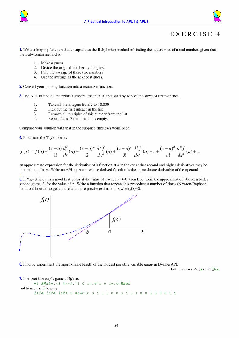
A Practical Introduction to APL 1 & APL 2
54
E X E R C I S E 4
1. Write a looping function that encapsulates the Babylonian method of finding the square root of a real number, given that
the Babylonian method is:
1. Make a guess
2. Divide the original number by the guess
3. Find the average of these two numbers
4. Use the average as the next best guess.
2. Convert your looping function into a recursive function.
3. Use APL to find all the prime numbers less than 10 thousand by way of the sieve of Eratosthanes:
1. Take all the integers from 2 to 10,000
2. Pick out the first integer in the list
3. Remove all multiples of this number from the list
4. Repeat 2 and 3 until the list is empty.
Compare your solution with that in the supplied dfns.dws workspace.
4. Find from the Taylor series
...)(!
)(..)(
!3
)()(
!2
)()(
!1
)()()(
3
33
2
22
+−
++−
+−
+−
+= adx
fd
n
axa
dx
fdaxa
dx
fdaxa
dx
dfaxafxf
n
nn
an approximate expression for the derivative of a function at a in the event that second and higher derivatives may be
ignored at point a. Write an APL operator whose derived function is the approximate derivative of the operand.
5. If f(x)=0, and a is a good first guess at the value of x when f(x)=0, then find, from the approximation above, a better
second guess, b, for the value of x. Write a function that repeats this procedure a number of times (Newton-Raphson
iteration) in order to get a more and more precise estimate of x when f(x)=0.
6. Find by experiment the approximate length of the longest possible variable name in Dyalog APL.
Hint: Use execute (–) and ŒWA.
7. Interpret Conway’s game of life as
†1 BMatŸ.^3 4=+/,¯1 0 1°.´¯1 0 1°.²›BMat
and hence use ÿ to play
life life life 5 8½40†0 0 1 0 0 0 0 0 1 0 1 0 0 0 0 0 0 1 1
A Practical Introduction to APL 1 & APL 2
55
E X E R C I S E 5
1. Write a function that takes an integer argument w, and returns a vector x of w equally spaced (dx) numbers between 5 and
5.
Big hint: x„((-w+1)+¼1+2×w)÷w÷5 ª dx„x[2]-x[1]
2. The Gaussian function
2
2
2
1)(
x
ex−
=π
ρ
maps values x ∈ ℝ into the interval 0 < ρ(x) ≤ (2π)-½
. ρ(x) may be interpreted in terms of the probability of obtaining x∈
X, given that X is a random variable that is normally distributed with mean value 0, standard deviation 1 and total
probability 1. Translate this function into APL and verify that
12
12
5
5
2
≈−
−∫ dxe
x
π.
Hint: +/dx×(÷(±2)*0.5)×*-(x*2)÷2
3. Write an operator E which takes an operand of a probability distribution ρ(x) and a vector argument x, and returns the
expectation of x under this distribution, given that mathematically
dxxxxE )()( ∫∞
∞−
= ρ .
Note that the vector x should be sorted before dx can be calculated.
Consider: +/dx×x×(÷(±2)*0.5)×*-(x*2)÷2
4. Write an operator Var which returns the variance of a vector of numbers, given that mathematically
)))((()( 2xExExVar −= .
Consider: E(¾-¨E ¾)°.×(¾-¨E ¾)
5. The APL primitive monadic function roll (?) takes an argument of any positive integer array, X, and returns a result that
contains integers, pseudo-randomly selected from the sets of integers ¼¨X with each integer in each population having an
equal (uniform) chance of being selected.
Write a monadic function called U that takes a positive integer vector argument (corresponding to the shape of some
numeric array) and returns a vector containing half the number of elements in the original numeric array composed of a
uniform distribution of numbers between 0 and 1.
Big hint: U„{(?(—(×/¾)÷2)½¯1+2*31)÷¯1+2*31}
6. In 1958, Box and Müller published an algorithm for transforming a uniform distribution of random numbers into a normal
distribution of random numbers by inverting the Gaussian function continued into ℂ : 22
121 )ln(2iy
eyixxπ−=+ .
This takes 2 real numbers y1 and y2 from independent uniform distributions and yields 2 numbers x1 and x2 from independent
normal distributions.
Write a monadic function called N which takes a positive integer argument and returns that many numbers normally
distributed around 0.
Big hint: N„{¾½†(›(¯2×µU ¾)*0.5)ר1 2±¨›±2×U ¾}

A Practical Introduction to APL 1 & APL 2
56

Certificate of A chievem ent
This is to certify that
_______________________________________________________________________________________
has successfully com pleted the introduction to =
APL 1 & APL 2
=
on ________________________________________
====Signed = ________________________________________
Instructor
Produced by ROBERTSON (Publishing), 15 Little Basing, Old Basing, Basingstoke, RG24 8AX, UK.