ANALYTICAL BEHAVIOR OF 2-D INCOMPRESSIBLE FLOW IN …

ANALYTICAL BEHAVIOR OF 2-D INCOMPRESSIBLE FLOW IN POROUSMEDIA

DIEGO CORDOBA, FRANCISCO GANCEDO AND RAFAEL ORIVE

Abstract. In this paper we study the analytic structure of a two-dimensional mass balance equation

of an incompressible fluid in a porous medium given by Darcy’s law. We obtain local existence anduniqueness by the particle-trajectory method and we present different global existence criterions.

These analytical results with numerical simulations are used to indicate nonformation of singularities.

Moreover, blow-up results are shown in a class of solutions with infinite energy.

1. Introduction

The dynamics of a fluid through a porous medium is a complex and not thoroughly understoodphenomenon [3, 16]. The purpose of the paper is to study a nonlinear two-dimensional mass balanceequation in porous media and the conditions of formation of singularities using analytical results andnumerical calculations.

In real applications, one might be interested in the transport of a dissolved contaminant in porousmedia where the contaminant is convected with the subsurface water [17]. For example, one is usuallyinterested in the time taken by the pollutant to reach the water table below. Such flows also occurin artificial recharge wells where water and (or) chemicals from the surface are transported intoaquifers. In this case, the chemicals may be the nutrients required for degradation of harmful pollutinghydrocarbons resident in the aquifer after a spillage.

We use Darcy’s law to model the flow velocities, yielding the following relationship between theliquid discharge (flux per unit area) v = (v1, v2) and the pressure gradient

v = −k (∇p+ gγρ) ,

where k is the matrix position-independent medium permeabilities in the different directions respec-tively divided by the viscosity, ρ is the liquid density, g is the acceleration due to gravity and thevector γ = (0, 1). While the Navier-Stokes equation and the Stokes equation are both microscopicequations, Darcy’s law gives the macroscopic description of a flow in a porous medium [3].

The free boundary problem given by an incompressible 2-D fluid through porous media with twodifferent constant densities and viscosities at each side of the interface is studied in [18, 1] (see referencestherein). Here, we analyze the dynamics of the density function ρ = ρ(x1, x2, t) with a regular initialdata ρ0 = ρ(x1, x2, 0).

The mass balance equation is given by

φDρ

Dt= φ

(∂ρ

∂t+ v · ∇ρ

)= 0,

where φ denotes the porosity of the medium. To simplify the notation, we consider k = g = φ = 1.Thus, our system of a two-dimensional mass balance equation in porous media (2DPM) is written as

Dρ

Dt= 0,(1.1)

v = − (∇p+ γρ) .(1.2)

We close the system assuming incompressibility, i.e.,

(1.3) divv = 0,

Date: May 31, 2006.Key words and phrases. Flows in porous media

2000 Mathematics Subject Classification. 76S05, 76B03, 65N06.The authors was partially supported by the grant MTM2005-05980 of the MEC (Spain) and S-0505/ESP/0158 of

the CAM (Spain). The third author was partially supported by the grant MTM2005-00714 of the MEC (Spain).

1

2 D. CORDOBA, F. GANCEDO AND R. ORIVE

therefore there exists a stream function ψ(x, t) such that

(1.4) v = ∇⊥ψ ≡(− ∂ψ

∂x2,∂ψ

∂x1

).

Computing the curl of equation (1.2), we get the Poisson equation for ψ

(1.5) −∆ψ =∂ρ

∂x1.

A solution of this equation is given by the convolution of the Newtonian potential with the function∂x1ρ

(1.6) ψ(x, t) = − 12π

∫R2

ln|x− y| ∂ρ∂y1

(y, t)dy, x ∈ R2.

Thus, the velocity v can be recovered from ψ by the operator ∇⊥ by the two equivalent formulas

v(x, t) =∫

R2K(x− y)∇⊥ρ(y, t)dy, x ∈ R2,(1.7)

v(x, t) = PV∫

R2H(x− y) ρ(y, t)dy − 1

2(0, ρ(x)) , x ∈ R2,(1.8)

where the kernels K(·) and H(·) are defined by

K(x) = − 12π

x1

|x|2and H(x) =

12π

(−2

x1x2

|x|4,x2

1 − x22

|x|4

).(1.9)

Differentiating the equation (1.1), we obtain the evolution equation for

∇⊥ρ ≡(− ∂ρ

∂x2,∂ρ

∂x1

)(1.10)

which is given by

(1.11)D∇⊥ρDt

= (∇v)∇⊥ρ.

Taking the divergence of the equation (1.2), we get

−∆p =∂ρ

∂x2

and the pressure can be obtained as in (1.6).The objective of this work is to analyze the behavior of the solutions of the system 2DPM (1.1)-

(1.3). First, we present the existence of singularities in a class of solutions with infinite energy in2DPM (see Proposition 2.2 and Remark 2.3).

In the case of solutions with regular initial data and finite energy, we get local well-posedness usingthe classical particle trajectories method. We illustrate a criterion of global existence solutions viathe norm of the bounded mean oscillation space of (1.10). A similar result is known in the threedimensional Euler equation (3D Euler) [2]. Also, using the geometric structure of the level sets of thedensity (where ρ is constant) and the nonlinear evolution equations of the gradient of the arc lengthof the level sets, we establish that no singularities are possible under not very restrictive conditions.This result is comparable to the 3D Euler equations [7] and to the two-dimensional quasi geostrophicequation (2DQG) [8]. Applying these criterions, we find no evidence of formation of singularities inour numerical simulations.

The paper is organized as follows. In Section 2 we study the analytical behavior of solutionswith infinite energy. In Section 3 we prove the existence and uniqueness for the 2DPM, show acharacterization of formation of singular solutions and we present geometric constraints on singularsolutions. Finally, in Section 4 we illustrate two numerical examples in which the analytical resultsare applied to show nonsingular solutions.

ANALYTICAL BEHAVIOR OF 2DPM 3

2. Singularities with infinite energy

Let the stream function ψ be defined by

(2.1) ψ(x1, x2, t) = x2f(x1, t) + g(x1, t).

Note that under this hypothesis the solution of (1.1)–(1.3) has infinite energy.We reduce the equations (1.1)–(1.3) to other system with respect to the functions f and g. From

(1.5) the density, apart from a constant, satisfies

(2.2) ρ(t, x1, x2) = −x2∂f

∂x1(x1, t)−

∂g

∂x1(x1, t) = −x2fx1 − gx1 ,

and, by (1.4), v verifies

(2.3) v(t, x1, x2) =(−f(x1, t), x2

∂f

∂x1(x1, t) +

∂g

∂x1(x1, t)

)= (−f, x2fx1 + gx1).

Therefore, the system (1.1)–(1.3) under the hypothesis (2.1) is equivalent to

(fx)t = ffxx − (fx)2,(2.4)(gx)t = fgxx − fxgx.(2.5)

(Here and in the sequel of the section, we denote with subscript the derivatives with respect to x.)We note the non-linear character of the first equation. Thus, our study of formation of singularitiesis concentrated in the solutions of (2.4). The function g depends implicitly on f in equation (2.5).

Now, we show that the system (2.4) and (2.5) is local well posed in the Sobolev spaces Hk0 (0, 1).

Lemma 2.1. Let f0 = f(x, 0) and g0 = g(x, 0) satisfy f0x , g

0x ∈ Hk

0 (0, 1) with k ≥ 1. Then, thereexists T > 0 such that fx, gx ∈ C1([0, T ];Hk

0 (0, 1)) are the unique solution of (2.4)–(2.5).

Proof. By (2.4) and integrating by parts, we have

12d

dt‖fx‖2L2 =

∫ 1

0

fxffxx −∫ 1

0

f3x = −3

2

∫ 1

0

f3x ≤ C‖fx‖L∞‖fx‖2L2 ≤ C‖fx‖3H1

0.

Analogously,

12d

dt‖fxx‖2L2 = −

∫ 1

0

f2xxfx −

∫ 1

0

fxxffxxx = −12

∫ 1

0

f2xxfx ≤ C‖fx‖L∞‖fxx‖2L2 ≤ C‖fx‖3H1

0.

We can repeat for all k ≥ 1 and we obtain

12d

dt‖fx‖2Hk

0≤ C‖fx‖3Hk

0.

Integrating in time, we get

‖fx‖Hk0≤

‖f0x‖Hk

0

1− Ct‖f0x‖Hk

0

.

On the other hand, by (2.4) and integrating by parts, we have for gx the following inequalities

12d

dt‖gx‖2L2 =

∫ 1

0

gxgxxf −∫ 1

0

g2xfx = −3

2

∫ 1

0

g2xfx ≤ ‖fx‖L∞‖gx‖2H1

0

and

12d

dt‖gxx‖2L2 =

∫ 1

0

gxxgxxxf −∫ 1

0

gxxgxfxx = −12

∫ 1

0

g2xxfx −

∫ 1

0

gxxgxfxx

≤ ‖fx‖L∞‖gxx‖2L2 + ‖gxx‖L2‖gx‖L∞‖fxx‖L2 ≤ ‖fx‖H10‖gx‖2H1

0.

Thus, we obtain using Gronwall’s Lemma

‖gx‖2Hk0≤ ‖g0

x‖2Hk0

exp(C

∫ t

0

‖fx‖Hk0ds

)and we have existence up to a time T = T (‖f0

x‖Hk0).


In order to prove the uniqueness, let fx(x, t) = hx(x, t)−kx(x, t), with hx, kx two solutions of (2.4)with the same initial data f0

x . Since hx, kx satisfy (2.4) and integrating by parts, we have

12d

dt‖fx‖2L2 =

∫ 1

0

fx(hhxx − kkxx)−∫ 1

0

fx(h2x − k2

x)

=∫ 1

0

fxhfxx +∫ 1

0

fxfkxx −∫ 1

0

(fx)2(hx + kx)

= −12

∫ 1

0

(fx)2hx +∫ 1

0

fxfkxx −∫ 1

0

(fx)2(hx + kx).

Thus, we get

12d

dt‖fx‖2L2 ≤ ‖kxx‖L2‖fx‖L2‖f‖L∞ + C(‖hx‖L∞ + ‖kx‖L∞)‖fx‖2L2

≤ C(‖hx‖H10

+ ‖kx‖H10)‖fx‖2L2

and using Gronwall’s Lemma it follows hx = kx. Finally, we conclude the uniqueness of gx since (2.5)is a linear differential equation .

The following result shows that the solution of (2.4) blows up in finite time under certain conditionson the initial data.

Proposition 2.2. Let fx be a solution of (2.4) with initial data satisfies f0x ∈ H2

0 (0, 1) and minx f0x <

0. Then, ‖fx‖L∞ blows up in finite time T = −1/minx f0x .

Proof. By the local existence result, we have fx ∈ C1([0, T ];H2) ⊂ C1([0, T ] × [0, 1]). We considerthe application m : [0, T ] → R defined by m(t) = minx fx(x, t) = fx(xt, t). By Rademacher Theorem,it follows that m is differentiable at almost every point.

First, we calculate the derivative of m as in [5, 9]. Let s be a point of differentiability of m(t), thenfor τ > 0

m′(s) = limτ→0

m(s+ τ)−m(s)τ

= limτ→0

fx(xs+τ , s+ τ)− fx(xs, s)τ

= limτ→0

fx(xs+τ , s+ τ)− fx(xs, s+ τ)τ

+fx(xs, s+ τ)− fx(xs, s)

τ.

Since fx(x, s+ τ) reaches the minimum at the point xs+τ , we obtain

m′(s) ≤ limτ→0

fx(xs, s+ τ)− fx(xs, s)τ

= fxt(xs, s).

We compute the derivative with a sequence of negative τ < 0 and, by the sign of τ , we get the oppositeinequality and we conclude that

m′(s) = fxt(xs, s) almost everywhere.

We replace x for xs in (2.4) and yields

m′(s) = −f2x(xs, s) = −(m(s))2,

due to fxx(xs, s) = 0, and the proof follows.

Remark 2.3. There are other blow-up results with an initial data of lower regularity. In particular,we consider f0

x ∈ H10 and assuming that ∫ 1

0

f0x ≤ 0.

Thus, by (2.4), we have

d

dt

∫ 1

0

fx =∫ 1

0

ffxx −∫ 1

0

(fx)2 = −2∫ 1

0

(fx)2 ≥ −2(∫ 1

0

fx

)2

.

Defining

c(t) =∫fx,


and integrating, we get

c(t) ≤ c(0)1 + 2tc(0)

.

Then, c(t) blows up for c(0) < 0.In the case c(0) = 0, we have c′(t) < 0 for all t > 0, therefore, c(t) also blows up.

Remark 2.4. Let x1 = xt be the point such that

fx(xt, t) = minxfx(x, t),

and consider

x2 = 1− gx(xt, t)fx(xt, t)

.

Then, by (2.2), ρ(x1, x2, t) = −fx(xt, t) blows up in finite time by Proposition 2.2. Analogously, vdefined in (2.3) blows up in finite time.

3. Analysis of 2DPM with finite energy

3.1. Local existence of 2DPM. We derive a reformulation of the system as an integro-differentialequation for the particle trajectories. Given a smooth field v(x, t), the particle trajectories Φ(α, t)satisfy

dΦdt

(α, t) = v(Φ(α, t), t), Φ(α, t)|t=0 = α.(3.1)

The time-dependent map Φ(·, t) connects the Lagrangian reference frame (with the variable α) to theEulerian reference frame (with the variable x).

It is well known (Section 2.5 in [15]) that the equation (1.11) implies the following formula

∇⊥ρ(Φ(α, t), t) = ∇αΦ(α, t)∇⊥ρ0(α),

where ∇⊥ρ0 is the orthogonal gradient of the initial density. This last equality shows us that theorthogonal gradient of the density is stretched by ∇αΦ(α, t) along particle trajectories. We rewrite(1.7) as

(3.2) v(Φ(α, t), t) =∫

R2K(Φ(α, t)− Φ(β, t))∇αΦ(β, t)∇⊥ρ0(β)dβ.

We consider (3.1) as an ODE on a Banach space and using Picard Theorem the local in time existencefollows. This is proved analogously like the existence and uniqueness of solutions to the inviscid Eulerequation (see Section 4.1 in [15]). In fact, we consider ∇⊥ρ0 ∈ Cδ(R2), δ ∈ (0, 1). Let B be theBanach space defined by

B =Φ : R2 → R2 such that |Φ(0)|+ |∇αΦ|0 + |∇αΦ|δ <∞

,

where | · |0 is the L∞-norm and | · |δ is the Holder semi-norm. Define OM , the open set of B, as

OM =

Φ ∈ B| infα∈R2

det∇αΦ(α) >12

and |Φ(0)|+ |∇αΦ|0 + |∇αΦ|δ < M

.

The mapping v(Φ), defined by (3.2), satisfies the assumptions of the Picard theorem, i.e., v is boundedand locally Lipschitz continuous on OM . As a consequence, for any M > 0 there exists T (M) > 0and a unique solution

Φ ∈ C1((−T (M), T (M));OM )

to the particle trajectories (3.1, 3.2).

Remark 3.1. The 2DPM (1.1)–(1.3) has quantities conserved in time, the Lp norm of ρ for 1 ≤ p ≤∞, i.e.,

(3.3) ‖ρ(t)‖p = ‖ρ0‖p, ∀t > 0, 1 ≤ p ≤ ∞.

The velocity is obtained from ρ by (1.8). These operators are singular integrals with Calderon-Zygmundkernels (see [19]). Then for 1 < p <∞ the Lp norm of the velocity is bounded for any time t > 0.


3.2. Blow-up criterion. In order to estimate the growth of the Sobolev norms we use the spaceof functions of bounded mean oscillation (BMO) (see Chapter IV in [19] for an introduction of thisfunction space).

Theorem 3.2. Let ρ be the solution of equation (1.1)–(1.3) with initial data ρ0 ∈ Hs(R2) with s > 2.Then, the following are equivalent:

(A) The interval [0,∞) is the maximal interval of Hs existence for ρ.(B) The quantity

(3.4)∫ T

0

‖∇ρ‖BMO(t) dt <∞ ∀T > 0.

Proof. We denote the operator Λs by Λs ≡ (−∆)s/2. Since the fluid is incompressible, we have fors > 2

12d

dt‖Λsρ‖2L2 = −

∫R2

ΛsρΛs(v∇ρ) dx = −∫

R2Λsρ(Λs(v∇ρ)− vΛs(∇ρ)) dx,

≤ C‖Λsρ‖L2‖Λs(v∇ρ)− vΛs(∇ρ)‖L2 .

Using the following estimate (see [13])

‖Λs(fg)− fΛs(g)‖Lp ≤ c(‖∇f‖L∞‖Λs−1g‖Lp + ‖Λsf‖Lp‖g‖L∞

)1 < p <∞,

we obtain for p = 2

(3.5)12d

dt‖Λsρ‖2L2 ≤ C(‖∇v‖L∞ + ‖∇ρ‖L∞)‖Λsρ‖2L2 .

Integrating, we get for any t ≤ T

(3.6) ‖Λsρ‖L2 ≤ ‖Λsρ0‖L2 exp

(C

∫ T

0

(‖∇v‖L∞ + ‖∇ρ‖L∞)

).

Now, we use the following inequality given in [14]: Let f ∈ W s,p with 1 < p <∞ and s > 2/p, then,there exists a constant C=C(p,s) such that

(3.7) ‖f‖L∞ ≤ C(1 + ‖f‖BMO(1 + ln+‖f‖W s,p)),

where ln+(x) = max(0, ln(x)). Therefore, for s > 2 we have

‖∇ρ‖L∞ ≤ C(1 + ‖∇ρ‖BMO(1 + ln+‖∇ρ‖Hs−1)),

and from (3.6), we obtain that

(3.8) ‖∇ρ‖L∞ ≤ C(1 + ln+(‖ρ0‖Hs)‖∇ρ‖BMO

∫ T

0

(‖∇v‖L∞ + ‖∇ρ‖L∞) dt).

On the other hand, applying (3.7) for v ∈ Hs(R2), we have

‖∇v‖L∞ ≤ C(1 + ‖∇v‖BMO(1 + ln+‖∇v‖Hs−1)).

Since v satisfies (1.8) and the singular integrals are bounded operators in BMO (see [19]), we get

‖∇v‖L∞ ≤ C(1 + ‖∇ρ‖BMO(1 + ln+‖∇ρ‖Hs−1)),

and, using (3.6), we obtain

(3.9) ‖∇v‖L∞ ≤ C(1 + ln+(‖ρ0‖Hs)‖∇ρ‖BMO

∫ T

0

(‖∇v‖L∞ + ‖∇ρ‖L∞) dt).

From (3.8) and (3.9), follows

‖∇v‖L∞ + ‖∇ρ‖L∞ ≤ C(1 + ln+(‖ρ0‖Hs)‖∇ρ‖BMO

∫ T

0

(‖∇v‖L∞ + ‖∇ρ‖L∞) dt).

Applying Gronwall’s inequality, we have∫ T

0

(‖∇v‖L∞ + ‖∇ρ‖L∞) dt ≤ CT exp

(ln+(‖ρ0‖Hs)

∫ T

0

‖∇ρ‖BMO dt

),

and so (A) is a consequence of (B).


Finally, due to the inequality‖∇ρ‖BMO ≤ ‖∇ρ‖H1 ,

we conclude that (A) implies (B).

Remark 3.3. Using that‖∇ρ‖BMO ≤ C‖∇ρ‖L∞ ,

we get a blow-up characterization for numerical simulations.

3.3. Geometric constraints on singular solutions. From equation (1.1) it follows that the levelsets, ρ = constant, move with the fluid flow. Then ∇⊥ρ, defined in (1.10), is tangent to these levelsets.

For the 2DPM, the infinitesimal length of a level set for ρ is given by |∇⊥ρ| and from (1.11), theevolution equation for the infinitesimal arc length is given by

(3.10)D|∇⊥ρ|Dt

= L |∇⊥ρ|.

The factor L(x, t) is defined through by

(3.11) L(x, t) =Dη · η, η 6= 0,0, η = 0.

where the direction of ∇⊥ρ is denoted by

(3.12) η =∇⊥ρ|∇⊥ρ|

and D(x, t) is the symmetric part of the deformation matrix defined by

(3.13) D = (Dij) =[12

(∂vi

∂xj+∂vj

∂xi

)].

Now, we show a singularity criterion of 2DPM using the geometric structure of the level sets andmild hypotheses of the solutions. The theorem states below is analogous to 3D Euler [7] and to 2DQG[8].

Recall that η is the direction field tangent to the level sets of ρ defined (3.12). Analogously to [8],a set Ω is smoothly directed if there exists δ > 0 such that

(3.14) supx∈Ω

∫ T

0

‖∇η(·, t)‖2L∞(Bδ(Φ(x,t)))dt < ∞,

whereBδ(x) = y ∈ R2 : |x− y| < δ, Ω = x ∈ Ω; |∇ρ0(x)| 6= 0,

and Φ is the particle trajectories map. We define Ω(t) = Φ(Ω, t) and OT (Ω) the semi-orbit, i.e.,

OT (Ω) =⋃

0≤t≤T

t × Ω(t).

Theorem 3.4. If Ω is smoothly directed and

(3.15)∫ T

0

‖Rjρ‖L∞(t)dt < ∞, j = 1, 2, ∀T > 0,

where Rj denotes the Riesz transform in the direction xj, then

supOT (Ω)

|∇ρ(x, t)| < ∞.

Remark 3.5. Using the Remark 3.3, the previous theorem illustrates that finite-time singularities areimpossible in smoothly directed sets.

Proof. We show a similar formula of the level–set stretching factor L defined in (3.11). We start bycomputing the full gradient of the velocity v. From formula (1.7)

v(x) =∫

R2K(y)∇⊥ρ(x− y)dy,


we have∇v(x) =

∫R2K(y) (∇y∇⊥y ρ)(x− y)dy.

Take the integral as a limit as ε → 0 of integrals on |y| > ε and integrate by parts. In this fashion,we obtain the formula

(3.16) ∇v(x) =12π

PV∫

R2

(∇yρ(x− y)

)⊗ y

dy

|y|2− 1

2

0 0

∂ρ

∂x1(x)

∂ρ

∂x2(x)

,

where y is the unit vector defined by

y =(−2y1y2|y|2

,y21 − y2

2

|y|2

).

By definition of η in (3.12), we have η · ∇ρ = 0. Thus, computing we get

(3.17) L(x) =12π

PV∫

R2

(y · η(x)

)(η(x− y) · η⊥(x)

)|∇⊥ρ(x− y)| dy

|y|2.

Let be φ ∈ C∞c (R), φ ≥ 0, supp(φ) include in [−1, 1] and φ(s) = 1 in s ∈ [−1/2, 1/2]. Consider r > 0and decompose

L(x) = I1 + I2,

with

|I1| ≤12π

∣∣∣∣∫R2

(1− φ(|y|2/r2))(y · η(x)

)(∇⊥ρ(x− y) · η⊥(x)

) dy|y|2

∣∣∣∣ .Integrating by parts and using Cauchy-Schwartz inequality, we get

I1 ≤C

r2‖ρ‖L2 ≤ C

r2‖ρ0‖L2 .

We have for any |y| < r

|η(x− y) · η⊥(x)| ≤ |y|‖∇η‖L∞(Br(x)).

Applying this in the integral I2, we get

|I2| ≤∫|∇⊥ρ(x− y)|φ(|y|2/r2)dy

|y|‖∇η‖L∞(Br(x)).

We integrate by parts and decompose∫|∇⊥ρ(x− y)|φ(|y|2/r2)dy

|y|=∫ρ(x− y)∇⊥

(η(x− y)φ(|y|2/r2) 1

|y|

)dy = J1 + J2 + J3,

where

J1 =∫ρ(x− y)η(x− y)∇⊥(φ(|y|2/r2))dy

|y|,

J2 =∫ρ(x− y)∇⊥(η(x− y))φ(|y|2/r2)dy

|y|,

J3 =∫ρ(x− y)η(x− y)φ(|y|2/r2) (−y2, y1)

|y|3dy,

obtaining the following estimates

|J1| ≤ c‖ρ0‖L∞ and |J2| ≤ cr‖ρ0‖L∞‖∇η‖L∞(Br(x)).

The J3 term can be bounded using the identity

J3 = η(x)(−R2(ρ)(x), R1(ρ)(x)) + J4,

getting the following estimate for J4 in a similar way

|J4| ≤ r‖ρ0‖L∞‖∇η‖L∞(Br(x)) + r−1‖ρ0‖L2 .

Thus, we conclude the following estimate for the factor L:

|L(x)| ≤ c

[‖∇η‖L∞(Br(x)) max

j=1,2|Rj(ρ)|+ (r‖∇η‖L∞(Br(x)) + 1)(‖∇η‖L∞(Br(x))‖ρ0‖∞ + r−2‖ρ0‖2)

].


Using (3.10), we obtain by Gronwall’s lemma

supOT (Ω)

|∇ρ(x, t)| ≤ supΩ|∇ρ0| exp

(supy∈Ω

∫ T

0

M(t)dt),

where M(t) is defined by

M(t) = c

[‖∇η‖L∞(Br(x)) max

j=1,2|Rj(ρ)|+ (r‖∇η‖L∞(Br(x)) + 1)(‖∇η‖L∞(Br(x))‖ρ0‖∞ + r−2‖ρ0‖2)

],

with x = Φ(y, t). This concludes the proof of Theorem 3.4.

Remark 3.6. The condition (3.15) depending on the Riesz transform is different that in 2DQG (see[8]). This appears because the integral kernels (1.9) in 2DPM are different to the Kernels in 2DQG.

Now, we present a geometric conserved quantity that relates the curvature of the level sets and themagnitude |∇⊥ρ| in a similar way as in [6] (see references therein for more details). In particular, ifwe define the curvature of the level sets κ by

(3.18) κ(x, t) = (η · ∇η) · η⊥(x, t),

where η is the direction of ∇⊥ρ (see (3.12)), the following identity is satisfied

(3.19)D(κ|∇⊥ρ|)

Dt= ∇⊥ρ · ∇β

with

(3.20) β(x, t) = (η · ∇v) · η⊥(x, t).

Indeed, we now prove the identity (3.19). Since ∇⊥ρ and |∇⊥ρ| satisfies (1.11) and (3.10) respectively,we get

Dη

Dt= (∇v)η − L η.

Using (3.16), we obtainDη

Dt= β η⊥,

with β defined in (3.20). By the definition of κ (3.18) and the previous formula, we have

Dκ

Dt= ((∇v · η − L η)∇η) · η⊥ + (η · (β∇η⊥ + η⊥ ⊗∇β −∇η∇v)) · η⊥ − β(η · ∇η) · η

and, simplifying,Dκ

Dt= (∇β)η − Lκ.

Using this identity and (3.10), (3.19) is satisfied.

Remark 3.7. The integral of the quantity κ|∇⊥ρ| over a region given by two different level sets isconserved along the time, i.e.

(3.21)d

dt

( ∫x: C1≤ρ(x,t)≤C2

κ|∇⊥ρ| dx)

= 0.

This can be showed using the equation (3.19) and integrating by parts. Thus, in the case that |∇⊥ρ|is large by (3.21) the curvature κ is small if the level sets do not oscillate.

In all of our numerical experiments, we find no evidence of level set oscillations. On the contrary,we observe that the level sets are flattering where the gradient of ρ is growing.

4. Numerical simulations

Here we present two examples of numerical simulations for solutions of the 2-D mass balance inporous media with initial data in a period-cell [0, 2π]2. Although periodic boundary conditions arerather unphysical, which does not matter because we are interested in the small-scale structures.


Figure 1. Evolution of the density in the Case 1 for times t = 0, 3, 6, 8.5.

The numerical method. We solve the equations (1.1)–(1.3) numerically on a 2π-periodic cell witha spectral method with smoothing. This numerical method is similar to the scheme developed by Eand Shu [12] for incompressible flows and also used for the quasi-geostrophic active scalar in [8].

This algorithm is the standard Fourier-collocation method (see [4]) with smoothing. Roughly speak-ing, the differentiation operator is approximated in the Fourier space, while the nonlinear operationssuch as v · ∇ρ are done in the physical space.

We smooth the gradients adding filters to the spectral method in order for the numerical solutionsdo not degrade catastrophically. A way of adding the filters is to replace the Fourier multiplier ikj byikjϕ(|kj |) , where

ϕ(k) = e−a(k/N)b

, for |k| ≤ N.

Here N is the numerical cutoff for the Fourier modes and a, b is chosen with the machine accuracy(see [20]).

For the temporal discretization, we use Runge-Kutta methods of various order. In our case, wehave no explicit temporal dependence and we get a Runge-Kutta method of order 4 that requires atmost three levels of storage, see in [4] p. 109.

We present the numerical approximation with an initial resolution of (256)2 Fourier modes. Werefine this resolution when the growth of ‖∇ρ‖L∞ is substantial to give additional insight preservingthe relation space-time. We conclude our numerical simulations with a resolution of (8192)2 Fouriermodes.

The computational part of this work was performed on HPC320 (cluster of 8 SMP servers with 32processors Alpha EV68 1 GHz) of the Centro de Supercomputacion de Galicia (CESGA). We usedthe MATLAB routines to obtain the calculations.


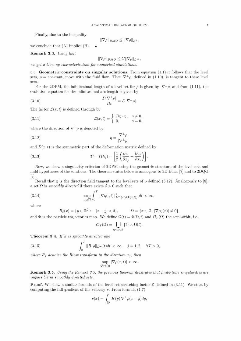
Figure 2. Evolution of the level sets -0.999, -0.99 (on the left of the figure) and0.99, 0.999 (on the right) of the density in the Case 1 for times t = 0, 3, 6.

Figure 3. Evolution of the L∞-norms of ∇ρ, the velocity v and the Riesz transforms(R1ρ,R2ρ) for the Case 1.

Case 1. We consider the initial datum

ρ(x1, x2) = sin(x1) sin(x2).

The time step is 4t = 0.025 from t = 0 to t = 4.0 with a = 4.5 and b = 2.3, stopping the experimentwith 4t = 0.00125 and a = 9.1, b = 7.1. During the simulation the ratio h/4t is preserved getting afiner resolution as the gradients are growing. In this way the method conserves in time the L∞-normof the density.

Figure 1 presents the density at times t = 0, 3, 6, 8.5 with a numerical resolution of (256)2, (256)2,(1024)2, (4096)2, respectively. The initial data has a hyperbolic saddle point that does not present anonlinear behavior as time evolves. In all our numerical simulations we do not find any saddle pointstructures that present stronger front formation than in case 2 (see Figure 5). Nevertheless, the case 1


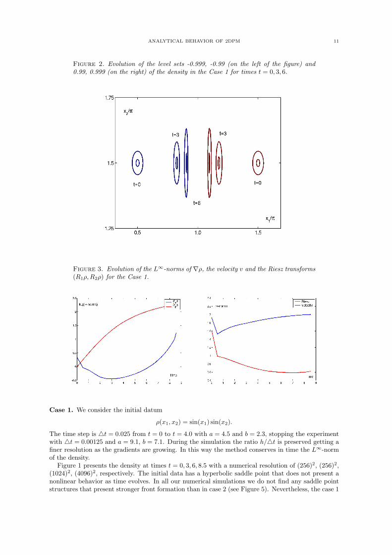
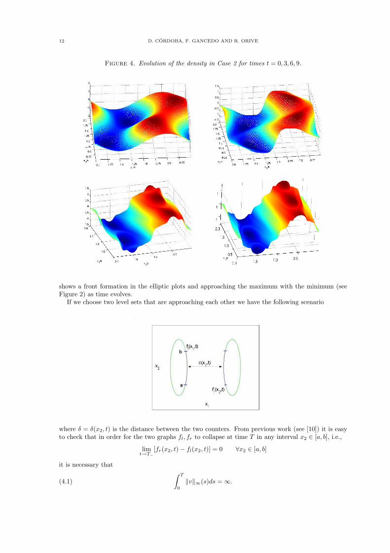
Figure 4. Evolution of the density in Case 2 for times t = 0, 3, 6, 9.

shows a front formation in the elliptic plots and approaching the maximum with the minimum (seeFigure 2) as time evolves.

If we choose two level sets that are approaching each other we have the following scenario

where δ = δ(x2, t) is the distance between the two counters. From previous work (see [10]) it is easyto check that in order for the two graphs fl, fr to collapse at time T in any interval x2 ∈ [a, b], i.e.,

limt→T−

[fr(x2, t)− fl(x2, t)] = 0 ∀x2 ∈ [a, b]

it is necessary that

(4.1)∫ T

0

‖v‖∞(s)ds = ∞.


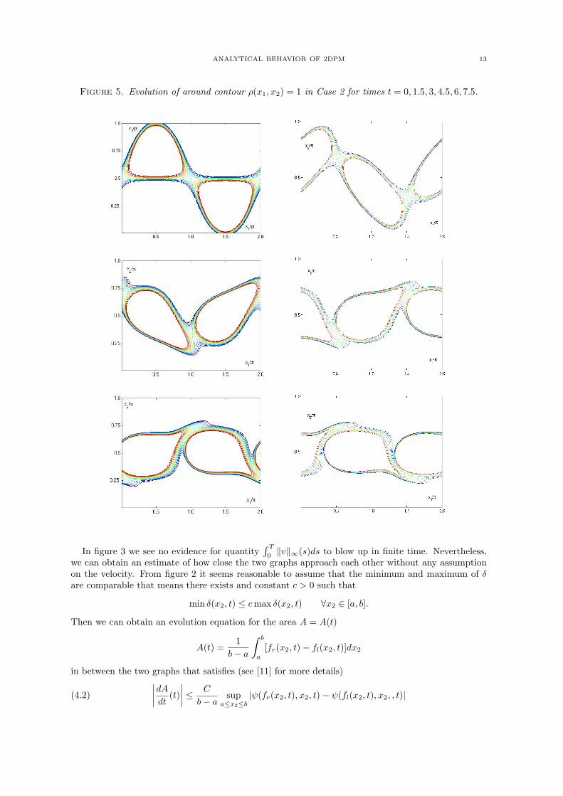
Figure 5. Evolution of around contour ρ(x1, x2) = 1 in Case 2 for times t = 0, 1.5, 3, 4.5, 6, 7.5.

In figure 3 we see no evidence for quantity∫ T

0‖v‖∞(s)ds to blow up in finite time. Nevertheless,

we can obtain an estimate of how close the two graphs approach each other without any assumptionon the velocity. From figure 2 it seems reasonable to assume that the minimum and maximum of δare comparable that means there exists and constant c > 0 such that

min δ(x2, t) ≤ cmax δ(x2, t) ∀x2 ∈ [a, b].

Then we can obtain an evolution equation for the area A = A(t)

A(t) =1

b− a

∫ b

a

[fr(x2, t)− fl(x2, t)]dx2

in between the two graphs that satisfies (see [11] for more details)

(4.2)∣∣∣∣dAdt (t)

∣∣∣∣ ≤ C

b− asup

a≤x2≤b|ψ(fr(x2, t), x2, t)− ψ(fl(x2, t), x2, , t)|


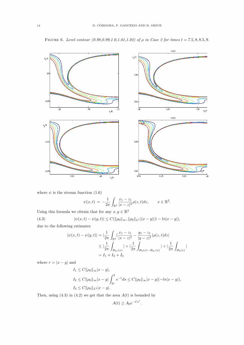
Figure 6. Level contour (0.98,0.99,1.0,1.01,1.02) of ρ in Case 2 for times t = 7.5, 8, 8.5, 9.

where ψ is the stream function (1.6)

ψ(x, t) = − 12π

∫R2

x1 − z1|x− z|2

ρ(z, t)dz, x ∈ R2.

Using this formula we obtain that for any x, y ∈ R2

(4.3) |ψ(x, t)− ψ(y, t)| ≤ C(‖ρ0‖∞, ‖ρ0‖L2)|x− y|(1− ln|x− y|),

due to the following estimates

|ψ(x, t)− ψ(y, t)| = | 12π

∫R2

(x1 − z1|x− z|2

− y1 − z1|y − z|2

)ρ(z, t)dz|

≤ | 12π

∫B2r(x)

|+ | 12π

∫B2(x)−B2r(x)

|+ | 12π

∫B2(x)

|

= I1 + I2 + I3

where r = |x− y| and

I1 ≤ C‖ρ0‖∞|x− y|,

I2 ≤ C‖ρ0‖∞|x− y|∫ 2

2r

s−1ds ≤ C‖ρ0‖∞|x− y|(−ln|x− y|),

I3 ≤ C‖ρ0‖L2 |x− y|.

Then, using (4.3) in (4.2) we get that the area A(t) is bounded by

A(t) ≥ A0e−Cet

.


Figure 7. Evolution of L∞-norms of ∇ρ, the velocity v and the Riesz transforms(R1ρ,R2ρ) for Case 2.

In order to apply the global solution criterion (Theorem 3.2), in Figure 3 is plotted the logarithm ofthe L∞-norms of ∂1ρ and ∂2ρ showing an exponential growth. The hypothesis (3.15) of the Theorem(3.4) is checked in this example (see Figure 3), so that using this result no singularity is possible dueto the variation of the direction field tangent to the level sets is smooth.

Case 2. In this case, the initial datum is

ρ(x1, x2) = sin(x1) cos(x2) + cos(x1).

The time step is 4t = 0.025 from t = 0 to t = 4.5 with a = 4.5 and b = 2.3, stopping the experimentwith 4t = 0.001 and a = 11.4, b = 8. The L∞-norm is preserved during the simulation of this case.

Figure 4 presents the density at times t = 0, 3, 6, 9 with a numerical resolution of (256)2, (256)2,(1024)2, (8192)2, respectively. In Figure 7, we show log plots of max|∂x1ρ| and max|∂x2ρ|, where weobtain an analogous exponential growth as in the case 1. This growth is not sufficient to guarantee asingularity.

The initial data for the density scalar clearly has a hyperbolic saddle and the numerical solutiondevelops a front as time evolves (see Figures 5 and 6). We observe that the front does not developnonlinear or potentially singular structure as time evolves. Where η is smoothly directed we observethe highest growth of ‖∇ρ‖L∞ . Where η changes rapidly we obtain less growth of ‖∇ρ‖L∞ . Usingtheorem 3.4 we show no evidence of singularities.

References

[1] D. Ambrose, Well-posedness of Two-phase Hele-Shaw Flow without Surface Tension, Euro. Jnl of Applied Mathe-matics 15 (2004), 597–607.

[2] J. T. Beale, T. Kato and A. Majda, Remarks on the Breakdown of Smooth Solutions for the 3-D Euler Equations,

Commun. Math. Phys. 94 (1984), 61–66.[3] J. Bear, Dynamics of Fluids in Porous Media, American Elsevier, New York, 1972.

[4] C. Canuto, M. Y. Hussaini, A. Quarteroni and T. A. Zang, Spectral methods in fluid dynamics, Springer Series

in Computational Physics. Springer-Verlag, New York, 1988.[5] A. Constantin and J. Escher, Wave breaking for nonlinear nonlocal shallow water equations, Acta Math. 181

(1998), no. 2, 229–243.

[6] P. Constantin, Geometric statistics in turbulence, SIAM Rev. 36 (1994), 73–98.[7] P. Constantin, C. Fefferman and A. Majda, Geometric constraints on potential singularity formulation in the

3-D Euler equations, Commun. Partial Diff. Eq. 21 (1996), 559–571.[8] P. Constantin, A. Majda and E. Tabak, Formation of strong fronts in the 2-D quasigeostrophic thermal active

scalar, Nonlinearity 7 (1994), no. 6, 1495–1533.

[9] A. Cordoba and D. Cordoba, A maximum principle applied to Quasi-geostrophic equations, Comm. Math. Phys.249 (2004), no. 3, 511–528.

[10] D. Cordoba and C. Fefferman, Scalars convected by a two-dimensional incompressible flow, Comm. Pure Appl.

Math. 55 (2002), no. 2, 255–260.


[11] D. Cordoba and C. Fefferman, Growth of solutions for QG and 2D Euler equations J. Amer. Math. Soc. 15

(2002), no. 3, 665–670.

[12] W. E and C.-W. Shu, Small-scale structures in Boussinesq convection, Phys. Fluids 6 (1994), no. 1, 49–58.[13] T. Kato and Ponce, Commutator estimates and the Euler and Navier-Stokes equations, Communications on Pure

and Applied Mathematics 41 (1998), 891–907.

[14] H. Kozono and Y. Taniuchi, Limiting case of the Sobolev inequality in BMO, with application to the Eulerequations, Communications in Mathematical Physics 214 (2000), 191–200.

[15] A. J. Majda and A. L. Bertozzi, Vorticity and incompressible flow, Cambridge Univ. Press, Cambridge, 2002.

[16] D.A. Nield and A. Bejan, Convection in porous media, Springer-Verlag, New York, 1999.[17] M. Price, Introducing Groundwater, 2nd ed. Chapman & Hall, London, 1996.

[18] M. Siegel, R. E. Caflisch and S. Howison, Global existence, singular solutions, and ill-posedness for the Muskat

problem, Comm. Pure Appl. Math. 57 (2004), no. 10, 1374–1411.[19] E.M. Stein, Harmonic Analysis, Princeton University Press, Princeton, NJ, 1993.[20] H. Vandeven, Family of spectral filters for discontinuous problems, J, Sci. Comput. 6 (1991), 159–192.

Diego Cordoba and Francisco Gancedo

Departamento de MatematicasInstituto de Matematicas y Fısica Fundamental

Consejo Superior de Investigaciones CientıficasSerrano 123, 28006 Madrid, Spain.E-mail address: [email protected] and [email protected]

Rafael OriveDepartamento de Matematicas

Facultad de Ciencias

Universidad Autonoma de MadridCrta. Colmenar Viejo km. 15, 28049 Madrid, Spain.

E-mail address: [email protected]

Documents

ANALYTICAL BEHAVIOR OF 2-D INCOMPRESSIBLE FLOW IN …