Embed Size (px)
Citation preview
Algebraic Flux Correction III.
Incompressible Flow Problems
Stefan Turek1 and Dmitri Kuzmin2
1 Institute of Applied Mathematics (LS III), University of DortmundVogelpothsweg 87, D-44227, Dortmund, [email protected]
Summary. Algebraic FEM-FCT and FEM-TVD schemes are integrated into in-compressible flow solvers based on the ‘Multilevel Pressure Schur Complement’(MPSC) approach. It is shown that algebraic flux correction is feasible for noncon-forming (rotated bilinear) finite element approximations on unstructured meshes.Both (approximate) operator-splitting and fully coupled solution strategies are in-troduced for the discretized Navier-Stokes equations. The need for developmentof robust and efficient iterative solvers (outer Newton-like schemes, linear multigridtechniques, optimal smoothers/preconditioners) for implicit high-resolution schemesis emphasized. Numerical treatment of extensions (Boussinesq approximation, k− εturbulence model) is addressed and pertinent implementation details are given. Sim-ulation results are presented for three-dimensional benchmark problems as well asfor prototypical applications including multiphase and granular flows.
1 Introduction
For single-phase Newtonian fluids occupying a domain Ω ⊂ Rd (d = 2, 3)during the time interval (t0, t0+T ], the incompressible Navier-Stokes equations
∂u
∂t+ u · ∇u − ν∆u + ∇p = f , (1)
∇·u = 0
describe the laminar flow motion which depends on the physical properties ofthe fluid (viscosity ν) and, possibly, on some external forces f like buoyancy.The constant density ρ is “hidden” in the pressure p(x1, . . . , xd, t) which ad-justs itself instantaneously so as to render the time-dependent velocity fieldu(x1, . . . , xd, t) divergence-free. The problem statement is completed by spec-ifying the initial and boundary values for each particular application.
2 Stefan Turek and Dmitri Kuzmin
Although these equations seem to have a quite simple structure, they con-stitute a ‘grand challenge’ problem for mathematicians, physicists, and engi-neers alike, and they are (still) object of intensive research activities in the fieldof Computational Fluid Dynamics (CFD). Incompressible flow problems areespecially interesting from the viewpoint of applied mathematics and scientificcomputing, since they embody the whole range of difficulties which typicallyarise in the numerical treatment of partial differential equations. Therefore,they provide a perfect starting point for the development of reliable numericalalgorithms and efficient software for CFD simulations.
Specifically, the problems which scientists and engineers are frequentlyconfronted with, concern the following aspects:
• time-dependent partial differential equations in complex domains• strongly nonlinear and stiff systems of intricately coupled equations• convection-dominated transport at high Reynolds numbers (Re ≈ 1
ν )• saddle–point problems due to the incompressibility constraint• local changes of the problem character in space and time
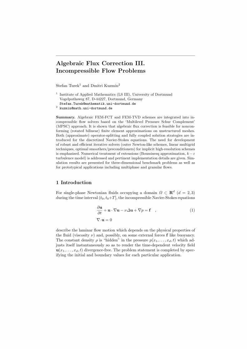
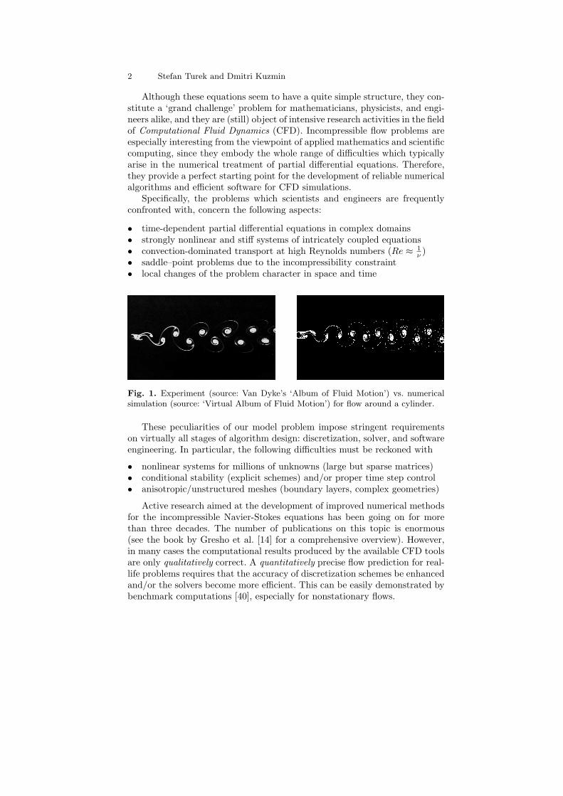
Fig. 1. Experiment (source: Van Dyke’s ‘Album of Fluid Motion’) vs. numericalsimulation (source: ‘Virtual Album of Fluid Motion’) for flow around a cylinder.
These peculiarities of our model problem impose stringent requirementson virtually all stages of algorithm design: discretization, solver, and softwareengineering. In particular, the following difficulties must be reckoned with
• nonlinear systems for millions of unknowns (large but sparse matrices)• conditional stability (explicit schemes) and/or proper time step control• anisotropic/unstructured meshes (boundary layers, complex geometries)
Active research aimed at the development of improved numerical methodsfor the incompressible Navier-Stokes equations has been going on for morethan three decades. The number of publications on this topic is enormous(see the book by Gresho et al. [14] for a comprehensive overview). However,in many cases the computational results produced by the available CFD toolsare only qualitatively correct. A quantitatively precise flow prediction for real-life problems requires that the accuracy of discretization schemes be enhancedand/or the solvers become more efficient. This can be easily demonstrated bybenchmark computations [40], especially for nonstationary flows.
Algebraic Flux Correction III 3
Moreover, a current trend in CFD is to combine the ‘basic’ Navier-Stokesequations (2) with more or less sophisticated engineering models from physicsand chemistry which describe industrial applications involving turbulence,multiphase flow, nonlinear fluids, combustion/detonation, free and movingboundaries, fluid-structure interaction, weakly compressible effects, etc. Theseextensions, some which will be discussed in the present chapter, have one thingin common: they require highly accurate and robust discretization techniquesas well as efficient solution algorithms for generalized Navier–Stokes–like sys-tems. In order to design and implement such powerful numerical methods forreal-life problems, many additional aspects need to be taken into account.
The main ingredients of an ‘ultimate’ CFD code are as follows
• advanced mathematical methods for PDEs (→ discretization)• efficient solution techniques for algebraic systems (→ solver)• reliable and hardware-optimized software (→ implementation)
If all of these components were available, the number of unknowns could besignificantly reduced (e.g., via adaptivity or a high-order approximation) and,moreover, discrete problems of the same size could be solved more efficiently.Hence, the marriage of optimal numerical methods and fast iterative solverswould make it possible to exploit the potential of modern computers to the fullextent and enhance the performance of incompressible flow solvers (improvethe MFLOP/s rates) by orders of magnitude. This is why these algorithmicaspects play an increasingly important role in contemporary CFD research.
In this contribution, we briefly review the Multilevel Pressure Schur Com-plement (MPSC) approach to solution of the incompressible Navier-Stokesequations and combine it with a FEM-FCT or FEM-TVD discretization ofthe (nonlinear) convective terms. We will explain the ramifications of thesenew (for the FEM community) algebraic high-resolution schemes as applied toincompressible flow problems and discuss a number of computational detailsregarding the efficient numerical solution of the resulting nonlinear and linearalgebraic systems. Furthermore, we will examine different coupling mecha-nisms between the ‘basic’ flow model (standard Navier-Stokes equations forthe velocity and pressure) and additional scalar or vector-valued transportequations. The primary goal is numerical simulation of high Reynolds numberflows which require special stabilization techniques and/or advanced turbu-lence models in order to capture the relevant physical effects.
On the other hand, we also consider incompressible flows at intermediateand low Reynolds numbers. They may call for a different solution strategybut the evolution of scalar variables (temperatures, concentrations, proba-bility densities, volume fractions, level set functions etc.) is still dominatedby transport operators. Moreover, the transported quantities are inherentlynonnegative in many cases. Therefore, standard discretization techniques mayfail, whereas the positivity-preserving FCT/TVD schemes persevere and yieldexcellent results as the numerical examples in this chapter will illustrate.
4 Stefan Turek and Dmitri Kuzmin
2 Discretization of the Navier-Stokes Equations
Let us discretize the Navier–Stokes equations (2) in time by a standard methodfor numerical solution of ODEs. For instance, an implicit θ–scheme (backwardEuler or Crank-Nicolson) or its three-step counterpart proposed by Glowinskiyields a sequence of boundary value problems of the form [47]
Given u(tn), compute u = u(tn+1) and p = p(tn+1) by solving
[I + θ∆t(u · ∇ − ν∆)]u + ∆t∇p = [I − θ1∆t(u(tn) · ∇ − ν∆)]u(tn)
+ θ2∆tf(tn+1) + θ3∆tf(tn) (2)
subject to the incompressibility constraint ∇ · u = 0.
For the spatial discretization, we choose a finite element approach. How-ever finite volumes, finite differences or spectral methods are possible, too.A finite element model of the Navier–Stokes equations is based on a suitablevariational formulation. On the finite mesh Th (triangles, quadrilaterals ortheir analogues in 3D) covering the domain Ω with local mesh size h, onedefines polynomial trial functions for velocity and pressure. These spaces Hh
and Lh should lead to numerically stable approximations as h → 0, i.e., theyshould satisfy the so-called Babuska–Brezzi (BB) condition [12]
minqh∈Lh
maxvh∈Hh
(qh,∇ · vh)
‖qh‖0 ‖∇vh‖0≥ γ > 0 (3)
with a mesh–independent constant γ. On the other hand, equal order interpo-lations for velocity and pressure are also admissible provided that an a prioriunstable discretization is stabilized in an appropriate way (see, e.g., [19]).
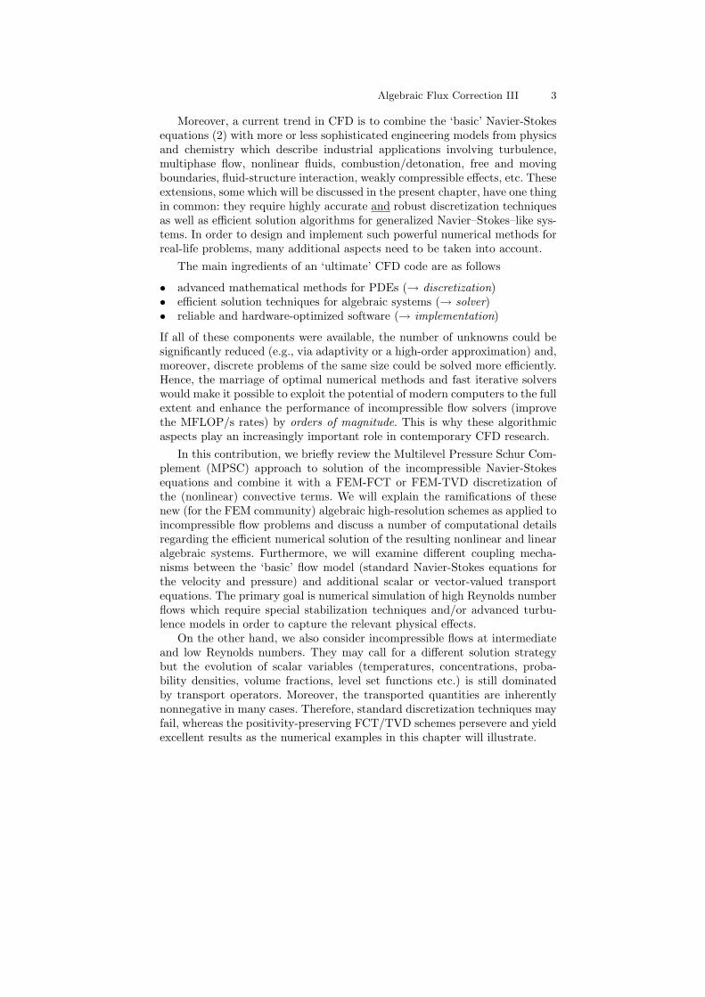
In what follows, we employ the stable Q1/Q0 finite element pair (rotatedbilinear/trilinear shape functions for the velocities, and a piecewise constantpressure approximation). In the two-dimensional case, the nodal values arethe mean values of the velocity vector over the element edges, and the meanvalues of the pressure over the elements (see Fig. 2).
p
u,v
u,v
u,v
u,v
Fig. 2. Nodal points of the nonconforming finite element pair Q1/Q0.
Algebraic Flux Correction III 5
This nonconforming finite element is a quadrilateral counterpart of thewell–known triangular Stokes element of Crouzeix–Raviart [6] and can easilybe defined in three space dimensions. A convergence analysis is given in [39]and computational results are reported in [42] and [43]. An important advan-tage of this finite element pair is the availability of efficient multigrid solverswhich are sufficiently robust in the whole range of Reynolds numbers even onnonuniform and highly anisotropic meshes [41],[47].
Using the notation u and p also for the coefficient vectors in the represen-tation of the approximate solution, the discrete version of problem (2) maybe written as a coupled (nonlinear) algebraic system of the form:
Given un and g, compute u = un+1 and p = pn+1 by solving
Au + ∆tBp = g , BT u = 0, where (4)
g = [M − θ1∆tN(un)]un + θ2∆tfn+1 + θ3∆tfn . (5)
Here M is the (consistent or lumped) mass matrix, B is the discrete gradientoperator, and −BT is the associated divergence operator. Furthermore,
Au = [M − θ∆tN(u)]u, N(u) = K(u) + νL, (6)
where L is the discrete Laplacian and K(u) is the nonlinear transport operatorincorporating a certain amount of artificial diffusion. In the sequel, we assumethat it corresponds to a FEM-TVD discretization of the convective term,although algebraic flux correction of FCT type or conventional stabilizationtechniques (upwinding, streamline diffusion) are also feasible.
The solution of nonlinear algebraic systems like (4) is a rather difficulttask and many aspects need to be taken into account:
• treatment of the nonlinearity: fully nonlinear solution by Newton–likemethods or iterative defect correction, explicit or implicit underrelaxation,monitoring of convergence rates, choice of stopping criteria etc.
• treatment of the incompressibility: strongly coupled approach (simul-taneous solution for u and p) vs. segregated algorithms based on operatorsplitting at the continuous or discrete level (classical projection schemes[3],[56] and pressure correction methods like SIMPLE [8],[34]).
• complete outer control: problem-dependent degree of coupling and/orimplicitness, optimal choice of linear algebra tools (iterative solvers andunderlying smoothers/preconditioners), automatic time step control etc.
This abundance of choices leads to a great variety of incompressible flowsolvers which are closely related to one another but exhibit considerable dif-ferences in terms of their stability, convergence, and efficiency. The MultilevelPressure Schur Complement (MPSC) approach outlined below makes it pos-sible to put many existing solution techniques into a common framework andcombine their advantages so as to obtain better run-time characteristics. Fora detailed presentation and a numerical study of the resulting schemes, theinterested reader is referred to the monograph by Turek [47].
6 Stefan Turek and Dmitri Kuzmin
3 Pressure Schur Complement Solvers
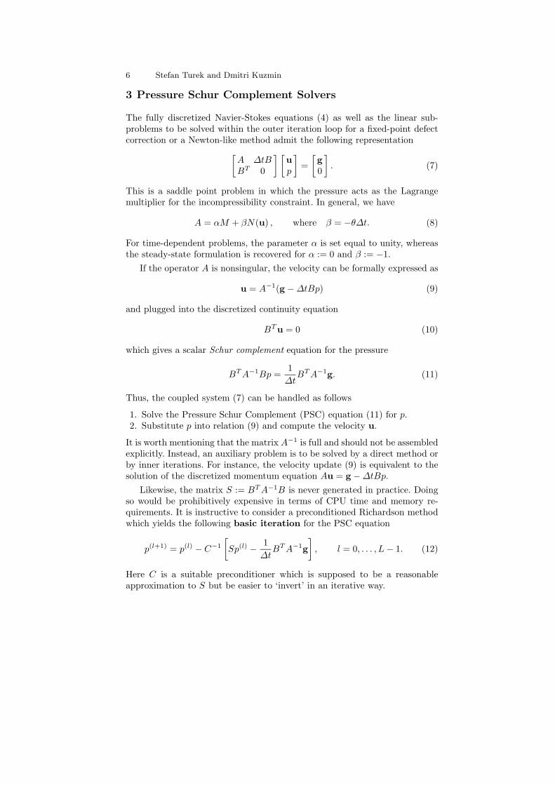
The fully discretized Navier-Stokes equations (4) as well as the linear sub-problems to be solved within the outer iteration loop for a fixed-point defectcorrection or a Newton-like method admit the following representation
[
A ∆tBBT 0
] [
up
]
=
[
g0
]
. (7)
This is a saddle point problem in which the pressure acts as the Lagrangemultiplier for the incompressibility constraint. In general, we have
A = αM + βN(u) , where β = −θ∆t. (8)
For time-dependent problems, the parameter α is set equal to unity, whereasthe steady-state formulation is recovered for α := 0 and β := −1.
If the operator A is nonsingular, the velocity can be formally expressed as
u = A−1(g − ∆tBp) (9)
and plugged into the discretized continuity equation
BT u = 0 (10)
which gives a scalar Schur complement equation for the pressure
BT A−1Bp =1
∆tBT A−1g. (11)
Thus, the coupled system (7) can be handled as follows
1. Solve the Pressure Schur Complement (PSC) equation (11) for p.2. Substitute p into relation (9) and compute the velocity u.
It is worth mentioning that the matrix A−1 is full and should not be assembledexplicitly. Instead, an auxiliary problem is to be solved by a direct method orby inner iterations. For instance, the velocity update (9) is equivalent to thesolution of the discretized momentum equation Au = g − ∆tBp.
Likewise, the matrix S := BT A−1B is never generated in practice. Doingso would be prohibitively expensive in terms of CPU time and memory re-quirements. It is instructive to consider a preconditioned Richardson methodwhich yields the following basic iteration for the PSC equation
p(l+1) = p(l) − C−1
[
Sp(l) − 1
∆tBT A−1g
]
, l = 0, . . . , L − 1. (12)
Here C is a suitable preconditioner which is supposed to be a reasonableapproximation to S but be easier to ‘invert’ in an iterative way.
Algebraic Flux Correction III 7
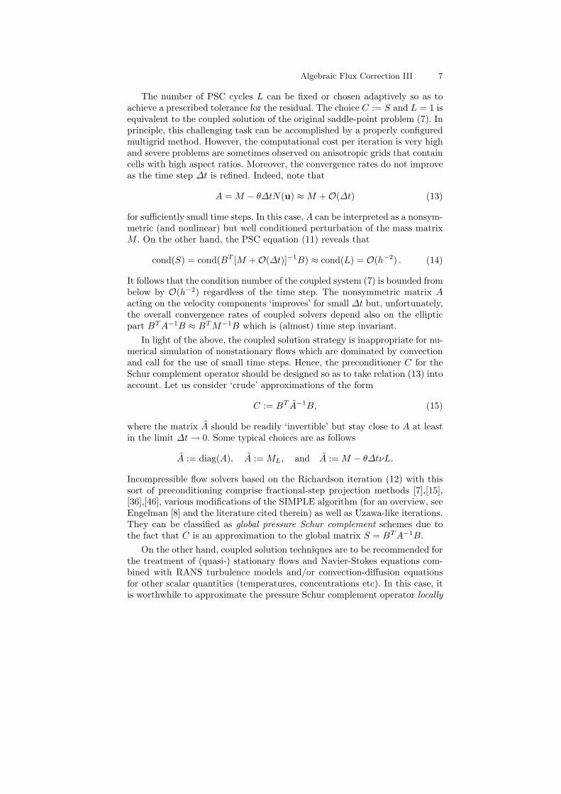
The number of PSC cycles L can be fixed or chosen adaptively so as toachieve a prescribed tolerance for the residual. The choice C := S and L = 1 isequivalent to the coupled solution of the original saddle-point problem (7). Inprinciple, this challenging task can be accomplished by a properly configuredmultigrid method. However, the computational cost per iteration is very highand severe problems are sometimes observed on anisotropic grids that containcells with high aspect ratios. Moreover, the convergence rates do not improveas the time step ∆t is refined. Indeed, note that
A = M − θ∆tN(u) ≈ M + O(∆t) (13)
for sufficiently small time steps. In this case, A can be interpreted as a nonsym-metric (and nonlinear) but well conditioned perturbation of the mass matrixM . On the other hand, the PSC equation (11) reveals that
cond(S) = cond(BT [M + O(∆t)]−1B) ≈ cond(L) = O(h−2) . (14)
It follows that the condition number of the coupled system (7) is bounded frombelow by O(h−2) regardless of the time step. The nonsymmetric matrix Aacting on the velocity components ‘improves’ for small ∆t but, unfortunately,the overall convergence rates of coupled solvers depend also on the ellipticpart BT A−1B ≈ BT M−1B which is (almost) time step invariant.
In light of the above, the coupled solution strategy is inappropriate for nu-merical simulation of nonstationary flows which are dominated by convectionand call for the use of small time steps. Hence, the preconditioner C for theSchur complement operator should be designed so as to take relation (13) intoaccount. Let us consider ‘crude’ approximations of the form
C := BT A−1B, (15)
where the matrix A should be readily ‘invertible’ but stay close to A at leastin the limit ∆t → 0. Some typical choices are as follows
A := diag(A), A := ML, and A := M − θ∆tνL.
Incompressible flow solvers based on the Richardson iteration (12) with thissort of preconditioning comprise fractional-step projection methods [7],[15],[36],[46], various modifications of the SIMPLE algorithm (for an overview, seeEngelman [8] and the literature cited therein) as well as Uzawa-like iterations.They can be classified as global pressure Schur complement schemes due tothe fact that C is an approximation to the global matrix S = BT A−1B.
On the other hand, coupled solution techniques are to be recommended forthe treatment of (quasi-) stationary flows and Navier-Stokes equations com-bined with RANS turbulence models and/or convection-diffusion equationsfor other scalar quantities (temperatures, concentrations etc). In this case, itis worthwhile to approximate the pressure Schur complement operator locally
8 Stefan Turek and Dmitri Kuzmin
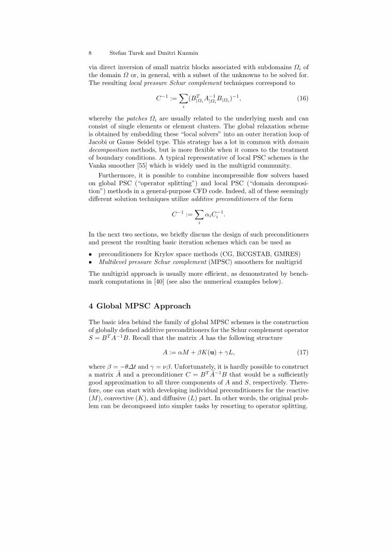
via direct inversion of small matrix blocks associated with subdomains Ωi ofthe domain Ω or, in general, with a subset of the unknowns to be solved for.The resulting local pressure Schur complement techniques correspond to
C−1 :=∑
i
(BT|Ωi
A−1|Ωi
B|Ωi)−1, (16)
whereby the patches Ωi are usually related to the underlying mesh and canconsist of single elements or element clusters. The global relaxation schemeis obtained by embedding these “local solvers” into an outer iteration loop ofJacobi or Gauss–Seidel type. This strategy has a lot in common with domaindecomposition methods, but is more flexible when it comes to the treatmentof boundary conditions. A typical representative of local PSC schemes is theVanka smoother [55] which is widely used in the multigrid community.
Furthermore, it is possible to combine incompressible flow solvers basedon global PSC (“operator splitting”) and local PSC (“domain decomposi-tion”) methods in a general-purpose CFD code. Indeed, all of these seeminglydifferent solution techniques utilize additive preconditioners of the form
C−1 :=∑
i
αiC−1i .
In the next two sections, we briefly discuss the design of such preconditionersand present the resulting basic iteration schemes which can be used as
• preconditioners for Krylov space methods (CG, BiCGSTAB, GMRES)• Multilevel pressure Schur complement (MPSC) smoothers for multigrid
The multigrid approach is usually more efficient, as demonstrated by bench-mark computations in [40] (see also the numerical examples below).
4 Global MPSC Approach
The basic idea behind the family of global MPSC schemes is the constructionof globally defined additive preconditioners for the Schur complement operatorS = BT A−1B. Recall that the matrix A has the following structure
A := αM + βK(u) + γL, (17)
where β = −θ∆t and γ = νβ. Unfortunately, it is hardly possible to constructa matrix A and a preconditioner C = BT A−1B that would be a sufficientlygood approximation to all three components of A and S, respectively. There-fore, one can start with developing individual preconditioners for the reactive(M), convective (K), and diffusive (L) part. In other words, the original prob-lem can be decomposed into simpler tasks by resorting to operator splitting.
Algebraic Flux Correction III 9
Let the inverse of C be composed from those of ‘optimal’ preconditionersfor the limiting cases of a divergence–free L2-projection (for small time steps),incompressible Euler equations, and a diffusion-dominated Stokes problem
C−1 = α′C−1M + β′C−1
K + γ′C−1L ≈ S−1, (18)
where the user-defined parameters (α′, β′, γ′) may toggle between (α, β, γ)and zero depending on the flow regime. Furthermore, it is implied that
CM is an ‘optimal’ approximation of the reactive part BT M−1B,
CK is an ‘optimal’ approximation of the convective part BT K−1B,
CL is an ‘optimal’ approximation of the diffusive part BT L−1B.
The meaning of ‘optimality’ has to be defined more precisely. Ideally,partial preconditioners should be direct solvers with respect to the under-lying subproblem. In fact, this may even be true for the fully ‘reactive’ caseS = BT M−1B. However, if these preconditioners are applied as smoothersin a multigrid context and the convergence rates are largely independent ofouter parameter settings as well as of the underlying mesh, then this is alreadysufficient for optimality of the global MPSC solver. Preconditioners CM , CK ,and CL satisfying this criterion are introduced and analyzed in [47].
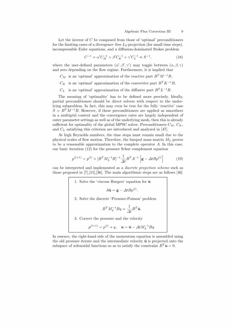
At high Reynolds numbers, the time steps must remain small due to thephysical scales of flow motion. Therefore, the lumped mass matrix ML provesto be a reasonable approximation to the complete operator A. In this case,our basic iteration (12) for the pressure Schur complement equation
p(l+1) = p(l) + [BT M−1L B]−1 1
∆tBT A−1
[
g − ∆tBp(l)]
(19)
can be interpreted and implemented as a discrete projection scheme such asthose proposed in [7],[15],[36]. The main algorithmic steps are as follows [46]
1. Solve the ‘viscous Burgers’ equation for u
Au = g − ∆tBp(l).
2. Solve the discrete ‘Pressure-Poisson’ problem
BT M−1L Bq =
1
∆tBT u.
3. Correct the pressure and the velocity
p(l+1) = p(l) + q, u = u − ∆tM−1L Bq.
In essence, the right-hand side of the momentum equation is assembled usingthe old pressure iterate and the intermediate velocity u is projected onto thesubspace of solenoidal functions so as to satisfy the constraint BT u = 0.
10 Stefan Turek and Dmitri Kuzmin
The matrix BT M−1L B corresponds to a mixed discretization of the Lapla-
cian operator [15] so that this method is a discrete analogue of the classicalprojection schemes derived by Chorin (p(0) = 0) and Van Kan (p(0) = p(tn))via operator splitting for the continuous problem [3],[56]. For an in-depth pre-sentation of continuous projection schemes we refer to [35],[36]. Our discreteapproach offers a number of important advantages including
• applicability to discontinuous pressure approximations• consistent treatment (no splitting) of boundary conditions• alleviation of spurious boundary layers for the pressure• convergence to the fully coupled solution as l increases• remarkable efficiency for nonstationary flow problems
On the other hand, discrete projection methods lack the inherent stabilizationmechanisms that make their continuous counterparts applicable to equal-orderinterpolations provided that the time step is not too small [35].
In our experience, it is often sufficient to perform exactly L = 1 pressureSchur complement iteration with just one multigrid sweep. Due to the factthat the numerical effort for solving the linear subproblems is insignificant,global MPSC methods are much more efficient than coupled solvers in the highReynolds number regime. However, they perform so well only for relativelysmall time steps, so that the more robust local MPSC schemes are to berecommended for low Reynolds number flows.
5 Local MPSC Approach
The local pressure Schur complement approach is tailored to solving ‘small’problems so as to exploit the fast cache of modern processors, in contrast tothe readily vectorizable global MPSC schemes. As already mentioned above,the basic idea is to subdivide the complete set of unknowns into patchesΩi and solve the local subproblems exactly within an outer block-Gauss-Seidel/Jacobi iteration loop. Typically, every patch (macroelement) for this‘domain decomposition’ method consists of one or several neighboring meshcells and the corresponding local ‘stiffness matrix’ Ci is given by
Ci :=
[
A|Ωi∆tB|Ωi
BT|Ωi
0
]
. (20)
Its coefficients (and hence the corresponding ‘boundary conditions’ for thesubdomains) are taken from the global matrices, whereby A may represent ei-ther the complete velocity matrix A or some approximation of it, for instance,the diagonal part diag(A). The local subproblems at hand are so small thatthey can be solved directly by Gaussian elimination. This is equivalent toapplying the inverse of Ci to a portion of the global defect vector.
Algebraic Flux Correction III 11
The elimination process leads to a fill-in of the matrix, which increases thestorage requirements dramatically. Thus, it is advisable to solve the equivalentlocal pressure Schur complement problem with the compact matrix
Si := BT|Ωi
A−1|Ωi
B|Ωi. (21)
In general, Si is a full matrix but it is much smaller than Ci, since onlythe pressure values are solved for. If the patch Ωi contains just a moderatenumber of elements, the pressure Schur complement matrix is likely to fit intothe processor cache. Having solved the local PSC subproblem, one can recoverthe corresponding velocity field as described in the previous section.
In any case, the basic iteration for a local MPSC method reads
[
u(l+1)
p(l+1)
]
=
[
u(l)
p(l)
]
− ω(l+1)
Np∑
i=1
[
A|Ωi∆tB|Ωi
BT|Ωi
0
]−1[
δu(l)i
δp(l)i
]
, (22)
where Np denotes the total number of patches, ω(l+1) is a relaxation param-eter, and the global defect vector restricted to a single patch Ωi is given by
[
δu(l)i
δp(l)i
]
=
([
A ∆tBBT 0
] [
u(l)
p(l)
]
−[
g0
])
|Ωi
. (23)
In practice, we solve the corresponding auxiliary problem
[
A|Ωi∆tB|Ωi
BT|Ωi
0
]
[
v(l+1)i
q(l+1)i
]
=
[
δu(l)i
δp(l)i
]
(24)
and compute the new iterates u(l+1)|Ωi
and p(l+1)|Ωi
as follows
[
u(l+1)|Ωi
p(l+1)|Ωi
]
=
[
u(l)|Ωi
p(l)|Ωi
]
− ω(l+1)
[
v(l+1)i
q(l+1)i
]
. (25)
This two-step relaxation procedure is applied to each patch, so some velocityor pressure components may end up being updated several times. The easiestway to obtain globally defined solution values at subdomain boundaries is tooverwrite the contributions of previously processed patches or to calculate anaverage over all patch contributions to the computational node.
The resulting local MPSC method corresponds to a simple block-Jacobiiteration for the mixed problem (4). Its robustness and efficiency can be easilyenhanced by computing the local defect vector (23) using the possibly updated
solution values rather than the old iterates u(l)|Ωi
and p(l)|Ωi
for the degrees of
freedom shared with other patches. This strategy is known as the block-Gauss-Seidel method. Its performance is superior to that of the block–Jacobi scheme,while the numerical effort is approximately the same (for a sequential code).
12 Stefan Turek and Dmitri Kuzmin
It is common knowledge that block-iterative methods of Jacobi and Gauss-Seidel type do a very good job as long as there are no strong mesh anisotropies.However, the convergence rates deteriorate dramatically for irregular triangu-lations which contain elements with high aspect ratios (for example, stretchedcells needed to resolve a boundary layer) and/or large differences between thesize of two neighboring elements. The use of ILU techniques alleviates thisproblem but is impractical for strongly coupled systems of equations. A muchbetter remedy is to combine the mesh elements so as to ‘hide’ the detrimentalanisotropies inside of the patches which are supposed to have approximatelythe same shape and size. Several adaptive blocking strategies for generationof such isotropic subdomains are described in [41],[47].
The global convergence behavior will be satisfactory because only the localsubproblems are ill-conditioned. Moreover, the size of these local problems isusually very small. Thus, the complete inverse of the matrix fits into RAM andsometimes even into the cache so that the use of fast direct solvers is feasible.Consequently, the convergence rates should be independent of grid distortionsand approach those for very regular structured meshes. If hardware–optimizedroutines such as the BLAS libraries are employed, then the solution of smallsubproblems can be performed very efficiently. Excellent convergence ratesand a high overall performance can be achieved if the code is properly tunedand adapted to the processor architecture in each particular case.
6 Multilevel Solution Strategy
Pressure Schur complement schemes constitute viable solution techniques assuch but they are particularly useful as smoothers for a multilevel algorithm,e.g., a geometric multigrid method. Let us start with explaining the typicalimplementation of such a solver for an abstract linear system of the form
ANuN = fN . (26)
It is assumed that there exists a hierarchy of levels k = 1, . . . , N which may becharacterized, for instance, by the mesh size hk. On each of these levels, oneneeds to assemble the matrix Ak and the right-hand side fk for the discreteproblem. We remark that only fN is available a priori, while the sequence ofresidual vectors fk for k < N is generated during the multigrid run.
The main ingredients of a (linear) multigrid algorithm are
• matrix–vector multiplication routines for the operators Ak, k ≤ N• an efficient smoother (basic iteration scheme) and a coarse grid solver• prolongation Ik
k−1 and restriction Ik−1k operators for grid transfer
Each k-level iteration MPSC(k, u0k, fk) with initial guess u0
k represents amultigrid cycle which yields an (approximate) solution of the linear systemAkuk = fk. On the first level, the number of unknowns is typically so smallthat the auxiliary problem can be solved directly: MPSC(1, u0
1, f1) = A−11 f1.
Algebraic Flux Correction III 13
For all other levels (k > 1), the following algorithm is adopted [47]
Step 1. Presmoothing
Apply m smoothing steps (PSC iterations) to u0k to obtain um
k .
Step 2. Coarse grid correction
Calculate fk−1 using the restriction operator Ik−1k via
fk−1 = Ik−1k (fk − Akum
k )
and let uik−1 (1 ≤ i ≤ p) be defined recursively by
uik−1 = MPSC(k − 1, ui−1
k−1, fk−1), u0k−1 = 0 .
Step 3. Relaxation and update
Calculate um+1k using the prolongation operator Ik
k−1 via
um+1k = um
k + αkIkk−1u
pk−1 , (27)
where the relaxation parameter αk may be fixed or chosen adaptivelyso as to minimize the error um+1
k − uk in an appropriate norm, forinstance, in the discrete energy norm
αk =(fk − Akum
k , Ikk−1u
pk−1)k
(AkIkk−1u
pk−1, I
kk−1u
pk−1)k
.
Step 4. Postsmoothing
Apply n smoothing steps (PSC iterations) to um+1k to obtain um+n+1
k .
After sufficiently many cycles on level N , the desired solution uN of the genericproblem (26) is recovered. In the framework of our multilevel pressure Schurcomplement schemes, there are (at least) two possible scenarios:
Global MPSC approach Solve the discrete problem (26) with
AN := BT A−1B, uN := p, fN :=1
∆tBT A−1g.
The basic iteration is given by (19) and equivalent to a discrete projection cy-cle, whereby the velocity field u is updated in a parallel manner (see above).The bulk of CPU time is spent on matrix-vector multiplications with theSchur complement operator S = BT A−1B which is needed for smoothing,defect calculation, and adaptive coarse grid correction. Unlike standard multi-grid methods for scalar problems, global MPSC schemes involve solutions of
14 Stefan Turek and Dmitri Kuzmin
a viscous Burgers equation and a Poisson-like problem in each matrix-vectormultiplication step (to avoid matrix inversion). In the case of highly nonsta-tionary flows, the overhead cost is insignificant but it becomes appreciable asthe Reynolds number decreases. Nevertheless, numerical tests indicate thatthe resulting multigrid solvers are optimal in the sense that the convergencerates are excellent and largely independent of mesh anisotropies.
Local MPSC approach Solve the discrete problem (26) with
AN :=
[
A ∆tBBT 0
]
, uN :=
[
up
]
, fN :=
[
g0
]
.
The basic iteration is given by (22) which corresponds to the block-Gauss-Seidel/Jacobi method. The cost-intensive part is the smoothing step, as inthe case of standard multigrid techniques for convection-diffusion equationsand Poisson-like problems. Local MPSC schemes lead to very robust solversfor coupled problems. This multilevel solution strategy is to be recommendedfor incompressible flows at low and intermediate Reynolds numbers.
Further algorithmic details (adaptive coarse grid correction, grid transferoperators, nonlinear iteration techniques, time step control, implementationof boundary conditions) and a description of the high-performance softwarepackage featflow based on MPSC solvers can be found in [47],[48]. Someprogramming strategies, data structures, and guidelines for the developmentof a hardware-oriented parallel code are presented in [49],[50],[51].
7 Coupling with Scalar Equations
Both global and local MPSC schemes are readily applicable to the Navier-Stokes equations coupled with various turbulence models and/or scalar con-servation laws for temperatures, concentrations, volume fractions, and otherscalar variables. In many cases, the quantities of interest must remain strictlynonnegative for physical reasons, and the failure to enforce the positivity con-straint for the numerical solution may have disastrous consequences. There-fore, a positivity-preserving discretization of convective terms is indispensablefor such applications. This prerequisite is clearly satisfied by the algebraicFEM-FCT and FEM-TVD schemes introduced in the previous chapters.
As a representative example of a two-way coupling between (2) and a scalartransport equation, we consider the well-known Boussinesq approximationfor natural convection problems. The nondimensional form of the governingequations for a buoyancy-driven incompressible flow reads [4]
∂u
∂t+ u · ∇u + ∇p = ν∆u + Teg, (28)
∂T
∂t+ u · ∇T = d∆T, ∇ · u = 0, (29)
Algebraic Flux Correction III 15
where u is the velocity, p is the deviation from hydrostatic pressure and Tis the temperature. The unit vector eg is directed ‘upward’ (opposite to thegravitational force) and the nondimensional diffusion coefficients
ν =
√
Pr
Ra, d =
√
1
RaPr
depend on the Rayleigh number Ra and the Prandtl number Pr. Details ofthis model and parameter settings for the MIT benchmark problem (naturalconvection in a differentially heated enclosure) can be found in [4].
7.1 Finite element discretization
After the discretization in space and time, we obtain a system of nonlinearalgebraic equations which can be written in matrix form as follows
Au(un+1)un+1 + ∆tMT Tn+1 + ∆tBpn+1 = fu, (30)
AT (un+1)Tn+1 = fT , BT un+1 = 0. (31)
Here and below the superscript n+1 refers to the time level, while subscriptsidentify the origin of discrete operators (u for the momentum equation and Tfor the heat conduction equation). Furthermore, the matrices Au and AT canbe decomposed into a reactive, convective, and diffusive part
Au(v) = αuMu + βuKu(v) + γuLu, (32)
AT (v) = αT MT + βT KT (v) + γT LT . (33)
Note that we have the freedom of using different finite element approximationsand discretization schemes for the velocity u and temperature T .
The discrete problem (30)–(31) admits the following representation
Au(un+1) ∆tMT ∆tB0 AT (un+1) 0BT 0 0
un+1
Tn+1
pn+1
=
fufT
0
(34)
and can be solved in the framework of a global or local MPSC method.
7.2 Global MPSC algorithm
Nonstationary flow configurations call for the use of operator splitting toolsfor the coupled system (34). This straightforward approach consists in solv-ing the Navier-Stokes equations for (u, p) and the energy equation for T in asegregated manner. The decoupled subproblems are embedded into an outeriteration loop and solved sequentially by a global MPSC method (discreteprojection) and an algebraic FCT/TVD scheme, respectively. For relativelysmall time steps, this strategy works very well, and simulation software can bedeveloped in a modular way making use of optimized multigrid solvers. More-over, it is possible to choose the time step individually for each subproblem.
16 Stefan Turek and Dmitri Kuzmin
In the simplest case (just one outer iteration per time step), the sequenceof algorithmic steps to be performed is as follows [52]
1. Compute u from the momentum equation
Au(u)u = fu − ∆tMT Tn − ∆tBpn.
2. Solve the discrete Pressure-Poisson problem
BT M−1L Bq =
1
∆tBT u.
3. Correct the pressure and the velocity
pn+1 = pn + q, un+1 = u − ∆tM−1L Bq.
4. Solve the convection-diffusion equation for T
AT (un+1)Tn+1 = fT .
Due to the nonlinearity of the discretized convective terms, iterative defectcorrection or a Newton-like method must be invoked in steps 1 and 4. Thisalgorithm combined with the nonconforming FEM discretization appears toprovide an ‘optimal’ flow solver for unsteady natural convection problems.
7.3 Local MPSC algorithm
Alternatively, a fully coupled solution of the problem at hand can be obtainedfollowing the local MPSC approach. To this end, a multigrid solver is appliedto the suitably linearized coupled system (34). Each outer iteration for thenonlinearity corresponds to the following solution update [41],[52]
u(l+1)
T (l+1)
p(l+1
=
u(l)
T (l)
p(l)
− ω(l+1)[F (σ, l)]−1
δu(l)
δT (l)
δp(l)
, (35)
where the global defect vector is given by the relation
δu(l)
δT (l)
δp(l)
=
Au(u(l)) ∆tMT ∆tB0 AT (u(l)) 0BT 0 0
u(l)
T (l)
p(l)
−
fufT
0
(36)
and the matrix to be inverted corresponds to the (approximate) Frechetderivative of the underlying PDE system such that [41],[47]
F (σ, l) =
Au(u(l)) + σR(u(l)) ∆tMT ∆tBσR(T (l)) AT (u(l)) 0BT 0 0
. (37)
Algebraic Flux Correction III 17
The nonlinearity of the governing equations gives rise to the ‘reactive’contribution R which represents a solution-dependent mass matrix and maycause severe convergence problems. This is why it is multiplied by the ad-justable parameter σ. The Newton method is recovered for σ = 1, while thevalue σ = 0 yields the fixed-point defect correction scheme. In either case, thelinearized problem is solved by a fully coupled multigrid solver equipped witha local MPSC smoother of ‘Vanka’ type [41]. As before, the matrix F (σ, l) isdecomposed into small blocks Ci associated with individual patches Ωi. Thesmoothing of the global residual vector is performed patchwise by solving thecorresponding local subproblems.
The size of the matrices to be inverted can be further reduced by resortingto the Schur complement approach. For simplicity, consider the case σ = 0(extension to σ > 0 is straightforward). It follows from (30)–(31) that
Tn+1 = A−1T fT , un+1 = A−1
u [fu − ∆tMT Tn+1 − ∆tBpn+1] (38)
and the discretized continuity equation can be cast into the form
BT un+1 = BT A−1u [fu − ∆tMT A−1
T fT − ∆tBpn+1] = 0 (39)
which corresponds to the pressure Schur complement equation
BT A−1u Bpn+1 = BT A−1
u
[
1
∆tfu − MT A−1
T fT
]
. (40)
Thus, highly efficient local preconditioners of the form (21) can be employedinstead of Ci. The converged solution pn+1 to the scalar subproblem (40) isplugged into (38) to obtain the velocity un+1 and the temperature Tn+1.
The advantages of the seemingly complicated local MPSC strategy are asfollows. First of all, steady-state solutions can be obtained without resorting topseudo-time-stepping. Moreover, the fully coupled treatment of dynamic flowsmakes it possible to use large time steps without any loss of robustness. Onthe other hand, the convergence behavior of multigrid solvers for the Newtonlinearization may turn out to be unsatisfactory and the computational costper outer iteration is rather high as compared to the global MPSC algorithm.The performance of both solution techniques as applied to the MIT benchmarkproblem is illustrated by the numerical results reported in [52].
8 Implementation of the k − ε Model
High-resolution schemes like FCT and TVD play an increasingly importantrole in simulation of turbulent flows. Flow structures that cannot be resolvedon the computational mesh activate the flux limiter which curtails the raw an-tidiffusion so as to filter out the small-scale fluctuations. Interestingly enough,the residual artificial viscosity provides an excellent subgrid scale model formonotonically integrated Large Eddy Simulation (MILES), see [2],[16].
18 Stefan Turek and Dmitri Kuzmin
In spite of recent advances in the field of LES and DNS (direct numericalsimulation), simpler turbulence models based on Reynolds averaging (RANS)still prevail in CFD software for simulation of industrial processes. In particu-lar, the evolution of the turbulent kinetic energy k and of its dissipation rateε is governed by two convection-dominated transport equations
∂k
∂t+ ∇ ·
(
ku − νT
σk∇k
)
= Pk − ε, (41)
∂ε
∂t+ ∇ ·
(
εu − νT
σε∇ε
)
=ε
k(C1Pk − C2ε), (42)
where u denotes the averaged velocity, νT = Cµk2/ε is the turbulent eddyviscosity and Pk = νT
2 |∇u + ∇uT |2 is the production term. For the standardk − ε model, the default values of the involved parameters are as follows
Cµ = 0.09, C1 = 1.44, C2 = 1.92, σk = 1.0, σε = 1.3.
The velocity field u is obtained from the incompressible Navier-Stokes equa-tions with ∇ · (ν + νT )[∇u + (∇u)T ] instead of ν∆u.
We remark that the transport equations for k and ε are strongly cou-pled and nonlinear so that their numerical solution is a very challenging task.Moreover, the discretization scheme must be positivity-preserving becausenegative values of the eddy viscosity are totally unacceptable. Unfortunately,implementation details and employed ‘tricks’ are rarely reported in the liter-ature, so that a novice to this area of CFD research often needs to reinventthe wheel. Therefore, we deem it appropriate to discuss the implementationof a FEM-TVD algorithm for the k − ε model in some detail.
8.1 Positivity-preserving linearization
The block-iterative algorithm proposed in [27],[28] consists of nested loopsso that the coupled PDE system is replaced by a sequence of linear sub-problems. The solution-dependent coefficients are ‘frozen’ during each outeriteration and updated as new values become available. The quasi-linear trans-port equations can be solved by an implicit FEM-FCT or FEM-TVD schemebut the linearization procedure must be tailored to the need to preserve thepositivity of k and ε in a numerical simulation. Due to the presence of sinkterms in the right-hand side of both equations, the positivity constraint maybe violated even if a high-resolution scheme is employed for the discretizationof convective terms. It can be proved that the exact solution to the k − εmodel remains nonnegative for positive initial data [32],[33] and it is essentialto guarantee that the numerical scheme will also possess this property.
Let us consider the following representation of the equations at hand [29]
∂k
∂t+ ∇ · (ku − dk∇k) + γk = Pk, (43)
∂ε
∂t+ ∇ · (εu − dε∇ε) + C2γε = C1Pk, (44)
Algebraic Flux Correction III 19
where the parameter γ = εk is proportional to the specific dissipation rate
(γ = Cµω). The turbulent dispersion coefficients are given by dk = νT
σkand
dε = νT
σε. By definition, the source terms in the right-hand side are nonnega-
tive. Furthermore, the parameters νT and γ must also be nonnegative for thesolution of the convection-reaction-diffusion equations to be well-behaved [5].In our numerical algorithm, their values are taken from the previous iterationand their positivity is secured as explained below. This linearization techniquewas proposed by Lew et al. [29] who noticed that the positivity of the laggedcoefficients is even more important than that of the transported quantities andcan be readily enforced without violating the discrete conservation principle.
Applying an implicit FCT/TVD scheme to the above equations, we obtaintwo nonlinear algebraic systems which can be written in the generic form
A(u(l+1))u(l+1) = B(u(l))u(l) + q(k), l = 0, 1, 2, . . . (45)
Here k is the index of the outermost loop in which the velocity u and thesource term Pk are updated. The index l refers to the outer iteration for thek − ε model, while the index m is reserved for inner flux/defect correctionloops. The structure of the matrices A and B is as follows:
A(u) = ML − θ∆t(K∗(u) + T ), (46)
B(u) = ML + (1 − θ)∆t(K∗(u) + T ), (47)
where K∗(u) is the LED transport operator incorporating nonlinear anti-diffusion and T denotes the standard reaction-diffusion operator which is asymmetric positive-definite matrix with nonnegative off-diagonal entries. It isobvious that the discretized production terms q(k) are also nonnegative. Thus,the positivity of u(l) is inherited by the new iterate u(l+1) = A−1(Bu(l) +q(k))provided that θ = 1 (backward Euler) or the time step is sufficiently small.
8.2 Positivity of coefficients
The predicted values k(l+1) and ε(l+1) are used to recompute the parameter
γ(l+1) for the next outer iteration (if any). The turbulent eddy viscosity ν(k)T is
updated in the outermost loop. In the turbulent flow regime νT ≫ ν and thelaminar viscosity ν can be neglected. Hence, we set νeff = νT , where the eddyviscosity νT is bounded from below by ν and from above by the maximumadmissible mixing length lmax (e.g. the width of the computational domain).Specifically, we define the limited mixing length l∗ as
l∗ =
αε if ε > α
lmax
lmax otherwise, where α = Cµk3/2 (48)
and use it to update the turbulent eddy viscosity νT in the outermost loop:
νT = maxν, l∗√
k (49)
20 Stefan Turek and Dmitri Kuzmin
as well as the parameter γ in each outer iteration for the k − ε model:
γ = Cµk
ν∗, where ν∗ = maxν, l∗
√k. (50)
In the case of a FEM-TVD method, the positivity proof is only valid for theconverged solution to (45) while intermediate solution values may be negative.Since it is impractical to perform many defect correction steps in each outeriteration, it is worthwhile to substitute k∗ = max0, k for k in formulae(48)–(50) so as to to prevent taking the square root of a negative number.Upon convergence, this safeguard will not make any difference, since k will benonnegative from the outset. The above representation of νT and γ makes itpossible to preclude division by zero and obtain bounded coefficients withoutmaking any ad hoc assumptions and affecting the actual values of k and ε.
8.3 Initial conditions
Another important issue which is seldom addressed in the CFD literature isthe initialization of data for the k − ε model. As a rule, it is rather difficultto devise a reasonable initial guess for a steady-state simulation or properinitial conditions for a dynamic one. The laminar Navier-Stokes equations (2)remain valid until the flow gains enough momentum for the turbulent effectsto become pronounced. Therefore, the k − ε model should be activated at acertain time t∗ > 0 after the startup.
During the ‘laminar’ initial phase (t ≤ t∗), a constant effective viscosityν0 is prescribed. The values to be assigned to k and ε at t = t∗ are uniquelydefined by the choice of ν0 and of the default mixing length l0 ∈ [lmin, lmax]where lmin corresponds to the size of the smallest admissible eddies:
k0 =
(
ν0
l0
)2
, ε0 = Cµk
3/20
l0at t ≤ t∗. (51)
This strategy was adopted because the effective viscosity ν0 and the mixinglength l0 are somewhat easier to estimate (at least for a CFD practitioner)than k0 and ε0. In any case, long-term simulation results are typically notvery sensitive to the choice of initial data.
8.4 Boundary conditions
At the inlet Γin, all velocity components and the values of k and ε are given:
u = g, k = cbc|u|2, ε = Cµk3/2
l0on Γin, (52)
where cbc ∈ [0.001, 0.01] is an empirical constant [5] and |u| =√
u · u is theEuclidean norm of the velocity. At the outlet Γout, the normal gradients of
Algebraic Flux Correction III 21
all scalar variables are required to vanish, and the ‘do-nothing’ [47] boundaryconditions are prescribed:
n · S(u) = 0, n · ∇k = 0, n · ∇ε = 0 on Γout. (53)
Here S(u) = −(
p + 23k
)
I +(ν +νT )[∇u+(∇u)T ] denotes the effective stresstensor. The numerical treatment of inflow and outflow boundary conditionsdoes not present any difficulty. In the finite element framework, relations (53)imply that the surface integrals resulting from integration by parts vanish anddo not need to be assembled.
At an impervious solid wall Γw, the normal component of the velocity mustvanish, whereas tangential slip is permitted in turbulent flow simulations. Theimplementation of the no-penetration (free slip) boundary condition
n · u = 0 on Γw (54)
is nontrivial if the boundary of the computational domain is not aligned withthe axes of the Cartesian coordinate system. In this case, condition (54)is imposed on a linear combination of several velocity components whereastheir boundary values are unknown. Therefore, standard implementation tech-niques for Dirichlet boundary conditions based on a modification of the cor-responding matrix rows [47] cannot be used.
In order to set the normal velocity component equal to zero, we nullify
the off-diagonal entries of the preconditioner A(u(m)) = a(m)ij in the defect
correction loop. This enables us to compute the boundary values of u explicitlybefore solving a sequence of linear systems for the velocity components:
a(m)ij := 0, ∀j 6= i, u∗
i := u(m)i + r
(m)i /a
(m)ii for xi ∈ Γw. (55)
Next, we project the predicted values u∗i onto the tangent vector/plane and
constrain the corresponding entry of the defect vector r(m)i to be zero
u(m)i := u∗
i − (ni · u∗i )ni, r
(m)i := 0 for xi ∈ Γw. (56)
After this manipulation, the corrected values u(m)i act as Dirichlet boundary
conditions for the solution u(m+1)i at the end of the defect correction step.
As an alternative to the implementation technique of predictor-correctortype, the projection can be applied to the residual vector rather than to thenodal values of the velocity:
a(m)ij := 0, ∀j 6= i, r
(m)i := r
(m)i − (ni · r(m)
i )ni for xi ∈ Γw. (57)
For Cartesian geometries, the algebraic manipulations to be performed affectjust the normal velocity component. Note that virtually no extra programmingeffort is required, which is a significant advantage as compared to anotherfeasible implementation based on local coordinate transformations during theelement-by-element matrix assembly [9].
22 Stefan Turek and Dmitri Kuzmin
8.5 Wall functions
To complete the problem statement, we still need to prescribe the tangentialstress as well as the boundary values of k and ε on Γw. Note that the equationsof the k − ε model are invalid in the vicinity of the wall where the Reynoldsnumber is rather low and viscous effects are dominant. In order to avoidthe need for resolution of strong velocity gradients, wall functions can bederived using the boundary layer theory and applied at an internal boundaryΓδ located at a distance δ from the solid wall Γw [31],[32],[33].
In essence, a boundary layer of width δ is removed from the actual com-putational domain Ω and the equations are solved in the reduced domain Ωδ
subject to the following empirical boundary conditions:
n · D(u) · t = −u2τ
u
|u| , k =u2
τ√
Cµ
, ε =u3
τ
κδon Γδ. (58)
Here D(u) = (ν +νT )[∇u+(∇u)T ] is the viscous part of the stress tensor, theunit vector t refers to the tangential direction, κ = 0.41 is the von Karmanconstant and uτ is the friction velocity which is assumed to satisfy
g(uτ ) = |u| − uτ
(
1
κlog y+ + 5.5
)
= 0 (59)
in the logarithmic layer, where the local Reynolds number y+ = uτ δν is in the
range 20 ≤ y+ ≤ 100, and be a linear function of y+ in the viscous sublayer,where y+ < 20. Note that u represents the tangential velocity as long as theno-penetration condition (54) is imposed on Γδ.
Equation (59) can be solved iteratively, e.g., by Newton’s method [31]:
ul+1τ = ul
τ − g(ulτ )
g′(ulτ )
= ulτ +
|u| − uτf(ulτ )
1/κ + f(ulτ )
, l = 0, 1, 2, . . . (60)
where the auxiliary function f is given by
f(uτ ) =1
κlog y+
∗ + 5.5, y+∗ = max
20,uτδ
ν
.
The friction velocity is initialized by the approximation
u0τ =
√
ν|u|δ
and no iterations are performed if it turns out that y+ =u0
τ δν < 20. In other
words, uτ = u0τ in the viscous sublayer. Moreover, we use y+
∗ = max20, y+in the Newton iteration to guarantee that the approximate solution belongsto the logarithmic layer and remains bounded for y+ → 0.
Algebraic Flux Correction III 23
The friction velocity uτ is plugged into (58) to compute the tangentialstress, which yields a natural boundary condition for the velocity. Integrationby parts in the weak form of the Navier-Stokes equations gives rise to a surfaceintegral over the internal boundary Γδ which contains the prescribed traction:
∫
Γδ
[n · D(u) · t] · v ds = −∫
Γδ
u2τ
u
|u| · v ds. (61)
The free slip condition (54) overrides the normal stress, and Dirichlet bound-ary conditions for k and ε are imposed in the strong sense. For further detailsregarding the implementation of wall laws we refer to [31],[32],[33].
8.6 Underrelaxation for outer iterations
Due to the intricate coupling of the governing equations, it is sometimesworthwhile to use a suitable underrelaxation technique in order to preventthe growth of numerical instabilities and secure the convergence of outer it-erations. This task can be accomplished by limiting the computed solutionincrements before applying them to the last iterate:
u(m+1) := u(m) + ω(m)(u(m+1) − u(m)), where 0 ≤ ω(m) ≤ 1. (62)
The damping factor ω(m) may be chosen adaptively so as to accelerate con-vergence and minimize the error in a certain norm [47]. However, fixed values(for example, ω = 0.8) usually suffice for practical purposes. The sort of un-derrelaxation can be used in all loops (indexed by k, l and m) and applied toselected dependent variables like k, ε or νT .
In addition, an implicit underrelaxation can be performed in m-loops byincreasing the diagonal dominance of the preconditioner [10],[34]
a(m)ii := a
(m)ii /α(m), where 0 ≤ α(m) ≤ 1. (63)
Of course, the scaling of the diagonal entries does not affect the convergedsolution. This strategy proves more robust than an explicit underrelaxation ofthe form (62). On the other hand, no underrelaxation whatsoever is neededfor moderate time steps which are typically used in dynamic simulations.
9 Adaptive Time Step Control
A remark is in order regarding the time step selection for implicit schemes.Unlike their explicit counterparts, they are unconditionally stable so thatthe time step is limited only by accuracy considerations (for nonstationaryproblems). Thus, it should be chosen adaptively so as to obtain a sufficientlygood approximation at the least possible cost. Many adaptive time steppingtechniques have been proposed in the literature. Most of them were originallydeveloped in the ODE context and are based on an estimate of the localtruncation error which provides a usable indicator for the step size control.
24 Stefan Turek and Dmitri Kuzmin
The ‘optimal’ value of ∆t should guarantee that the deviation of a user-defined functional J (pointwise solution values or certain integral quantitieslike lift and drag) from its exact value does not exceed a given tolerance
|J(u) − J(u∆t)| ≈ TOL. (64)
Assuming that the error at the time level tn is equal to zero, a heuristic errorindicator can be derived from asymptotic expansions for the numerical valuesof J computed using two different time steps. For instance, consider
J(u∆t) = J(u) + ∆t2e(u) + O(∆t)4,
J(um∆t) = J(u) + m2∆t2e(u) + O(∆t)4,
where m > 1 is an integer number (m = 2, 3). The error term e(v) is supposedto be independent of the time step and can be estimated as follows
e(u) ≈ J(um∆t) − J(u∆t)
(m2 − 1)∆t2.
For the relative error to approach the prescribed tolerance TOL as requiredby (64), the new time step ∆t∗ should be chosen so that
|J(u) − J(u∆t∗)| ≈(
∆t∗∆t
)2 |J(u∆t) − J(um∆t)|m2 − 1
= TOL.
The required adjustment of the time step is given by the formula
∆t2∗ = TOL(m2 − 1)∆t2
|J(u∆t) − J(um∆t)|.
Furthermore, the solution accuracy can be enhanced by resorting to Richard-son’s extrapolation (see any textbook on numerical methods for ODEs).
The above considerations may lack some mathematical rigor but never-theless lead to a very good algorithm for automatic time step control [47]
1. Make one large time step of size m∆t to compute um∆t.2. Make m small substeps of size ∆t to compute u∆t.3. Evaluate the relative changes, i. e., |J(u∆t) − J(um∆t)|.4. Calculate the ‘optimal’ value ∆t∗ for the next time step.5. If ∆t∗ ≪ ∆t, reject the solution and go back to step 1.6. Assign u := u∆t or perform Richardson’s extrapolation.
Note that the computational cost per time step increases significantly since thesolution um∆t may be as expensive to obtain as u∆t (due to slow convergence).On the other hand, adaptive time stepping contributes to the robustness of thecode and improves its overall efficiency as well as the credibility of simulationresults. Further algorithmic details for this approach can be found in [47].
Algebraic Flux Correction III 25
Another simple strategy for adaptive time step control was introduced byValli et al. [53],[54]. Their PID controller is based on the relative changes ofa suitable indicator variable (temperature distribution, concentration fields,kinetic energy, eddy viscosity etc.) and can be summarized as follows
1. Compute the relative changes of the chosen indicator variable u
en =||un+1 − un||
||un+1|| .
2. If they are too large (en > δ), reject un+1 and recompute it using
∆t∗ =δ
en∆tn.
3. Adjust the time step smoothly so as to approach the prescribedtolerance TOL for the relative changes
∆tn+1 =
(
en−1
en
)kP(
TOL
en
)kI(
e2n−1
enen−2
)kD
∆tn.
4. Limit the growth and reduction of the time step so that
∆tmin ≤ ∆tn+1 ≤ ∆tmax, m ≤ ∆tn+1
∆tn≤ M.
The default values of the PID parameters as proposed by Valli et al. [54] arekP = 0.075, kI = 0.175 and kD = 0.01. Unlike in the case of adaptive time-stepping techniques based on the local truncation error, there is no need forcomputing an extra solution with a different time step. Therefore, the cost ofthe feedback mechanism is negligible. Our own numerical studies [28] confirmthat this heuristic control strategy is very robust and efficient.
10 Numerical Examples
Flow around a cylinder. The first incompressible flow problem to be dealtwith is the well-known benchmark Flow around a cylinder developed in 1995for the priority research program “Flow simulation on high-performance com-puters” under the auspices of DFG, the German Research Association [40].This project was intended to facilitate the evaluation of various numerical al-gorithms for the incompressible Navier-Stokes equations in the laminar flowregime. A quantitative comparison of simulation results is possible on the ba-sis of relevant flow characteristics such as drag and lift coefficients, for whichsufficiently accurate reference values are available. Moreover, the efficiency ofdifferent solution techniques can be assessed in an objective manner.
26 Stefan Turek and Dmitri Kuzmin
Consider the steady incompressible flow around a cylinder with circularcross-section. An in-depth description of the geometrical details and bound-ary conditions for the 2D/3D case can be found in references [40],[47] whichcontain all relevant information regarding this benchmark configuration. Theflow at Re = 20 is actually dominated by diffusion and could be simulated bythe standard Galerkin method without any extra stabilization (as far as thediscretization is concerned; the iterative solver may require using a stabilizedpreconditioner). Ironically, it was this ‘trivial’ steady-state problem that hasled us to devise the multidimensional flux limiter of TVD type [24]. Both FCTschemes and slope limiter methods based on stencil reconstruction failed toconverge, so the need for a different limiting strategy was apparent.
Furthermore, it is instructive to study the interplay of finite element dis-cretizations for the convective and diffusive terms. As a matter of fact, dis-crete upwinding can be performed for the cumulative transport operator orjust for the convective part. In the case of the nonconforming Q1-elements,the discrete Laplacian operator originating from the Galerkin approximationof viscous terms is a positive-definite matrix but some of its off-diagonal coef-ficients are negative. Our numerical experiments indicate that it is worthwhileto leave it unchanged and start with a FEM-TVD discretization of the con-vective term. Physical diffusion can probably be taken into account afteralgebraic flux correction but the sums of upstream and downstream edge con-tributions Q± and P± for the node-oriented TVD limiter should be evaluatedusing the coefficients of the (antisymmetric) convective operator.
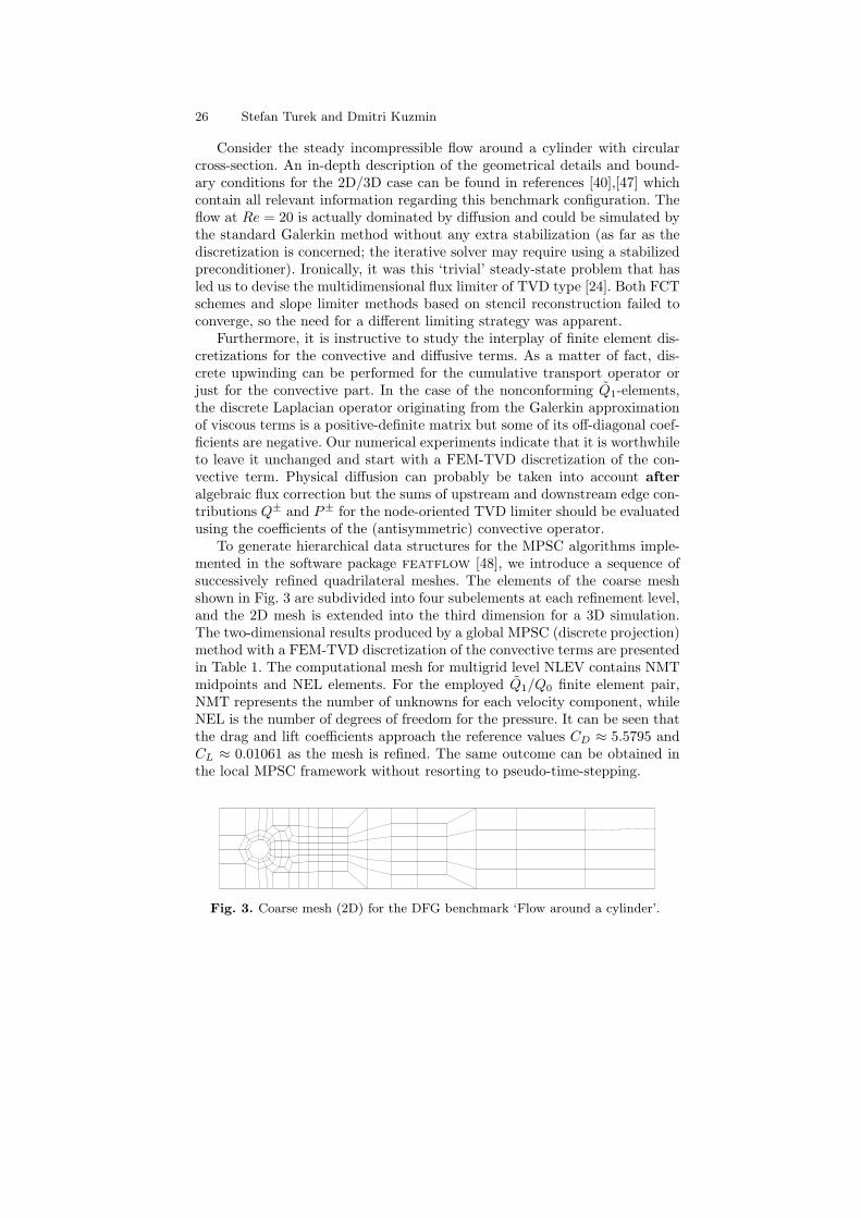
To generate hierarchical data structures for the MPSC algorithms imple-mented in the software package featflow [48], we introduce a sequence ofsuccessively refined quadrilateral meshes. The elements of the coarse meshshown in Fig. 3 are subdivided into four subelements at each refinement level,and the 2D mesh is extended into the third dimension for a 3D simulation.The two-dimensional results produced by a global MPSC (discrete projection)method with a FEM-TVD discretization of the convective terms are presentedin Table 1. The computational mesh for multigrid level NLEV contains NMTmidpoints and NEL elements. For the employed Q1/Q0 finite element pair,NMT represents the number of unknowns for each velocity component, whileNEL is the number of degrees of freedom for the pressure. It can be seen thatthe drag and lift coefficients approach the reference values CD ≈ 5.5795 andCL ≈ 0.01061 as the mesh is refined. The same outcome can be obtained inthe local MPSC framework without resorting to pseudo-time-stepping.
Fig. 3. Coarse mesh (2D) for the DFG benchmark ‘Flow around a cylinder’.
Algebraic Flux Correction III 27
Originally, stabilization of convective terms in the featflow package wasperformed using streamline diffusion or Samarski’s upwind scheme, wherebythe amount of artificial viscosity depends on the local Reynolds number andon the value of the user-defined parameter UPSAM as explained in [47],[48].Table 2 illustrates that drag and lift for UPSAM=0.1 and UPSAM=1.0 differappreciably, especially on coarse meshes. In the former case, both quantitiestend to be underestimated, while the latter parameter setting results in anunstable convergence behavior. Note that CL is negative (!) for NLEV=3.
Since the optimal value of the free parameter is highly problem-dependent,it is impossible to find from a priori considerations. In addition, Samarski’shybrid method is only suitable for intermediate and low Reynolds numbers, asit becomes increasingly diffusive and degenerates into the first-order upwindscheme in the limit of inviscid flow. By contrast, the accuracy of our FEM-TVD discretization does not degrade as Re → ∞. However, it does dependon the choice of the flux limiter (MC was employed in the above example)so the method is – arguably – not completely “parameter-free”. Moreover,the results are influenced by the type of Q1 basis functions (parametric ornon-parametric, with midpoint- or mean-value based degrees of freedom) aswell as by the approximations involved in the evaluation of CD and CL.
NLEV NMT NEL CD CL
3 4264 2080 5.5504 0.8708 · 10−2
4 16848 8320 5.5346 0.9939 · 10−2
5 66976 33280 5.5484 0.1043 · 10−1
6 267072 133120 5.5616 0.1056 · 10−1
7 1066624 532480 5.5707 0.1054 · 10−1
8 4263168 2129920 5.5793 0.1063 · 10−1
Table 1. Global MPSC method / TVD (MC limiter).
UPSAM=0.1 UPSAM=1.0
NLEV CD CL CD CL
3 5.4860 0.5302 · 10−2 5.9222 −0.3475 · 10−2
4 5.5076 0.9548 · 10−2 5.6525 0.6584 · 10−2
5 5.5386 0.1025 · 10−1 5.5736 0.1007 · 10−1
6 5.5581 0.1044 · 10−1 5.5658 0.1048 · 10−1
7 5.5692 0.1047 · 10−1 5.5718 0.1042 · 10−1
Table 2. Global MPSC method / Samarski’s upwind.
In Table 3, we present the drag and lift coefficients for a three-dimensionalsimulation of the flow around the cylinder. The hexahedral mesh for NLEV=4consists of 49,152 elements, which corresponds to 151,808 unknowns for eachvelocity component. In order to evaluate the performance of the global MPSC
28 Stefan Turek and Dmitri Kuzmin
solver and verify grid convergence, we compare the results to those obtainedon a coarser and a finer mesh. All numerical solutions were marched to thesteady state by the fully implicit backward Euler method. The discretizationof convective terms was performed using (i) finite volume upwinding (UPW),(ii) Samarski’s hybrid scheme (SAM), (iii) streamline diffusion stabilization(SD), and (iv) algebraic flux correction (TVD). This numerical study confirmsthat standard artificial viscosity methods are rather sensitive to the values ofthe empirical constants, whereas FEM-TVD performs remarkably well. Thereference values CD ≈ 6.1853 and CL ≈ 0.95 · 10−2 for this 3D configurationwere calculated in [20] by an isoparametric high-order FEM.
NLEV UPW-1st SAM-1.0 SD-0.25 SD-0.5 TVD/MC
3 6.08/ 1.01 5.72/ 0.28 5.78/-0.44 5.98/-0.52 5.80/ 0.36
4 6.32/ 1.20 6.07/ 0.62 6.13/ 0.26 6.26/ 0.18 6.14/ 0.46
5 6.30/ 1.20 6.14/ 0.83 6.17/ 0.70 6.23/ 0.64 6.18/ 0.80
Table 3. Global MPSC method: 3D simulation, CD/(CL · 100).
Backward facing step. Let us proceed to a three-dimensional test problemwhich deals with a turbulent flow over a backward facing step at Re = 44, 000,see [31] for details. Our objective is to validate the implementation of thek − ε model as described above. As before, the incompressible Navier-Stokesequations are discretized in space using the BB-stable nonconforming Q1/Q0
finite element pair, while conforming Q1 (trilinear) elements are employedfor the turbulent kinetic energy and its dissipation rate. All convective termsare handled by the fully implicit FEM-TVD method. The velocity-pressurecoupling is enforced in the framework of a global MPSC formulation.
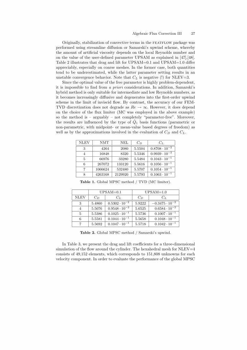
Standard wall laws are applied on the boundary except for the inlet andoutlet. The stationary distribution of k and ε in the middle cross-section(z = 0.5) is displayed in Fig. 4. The variation of the friction coefficient
cf =2τw
ρ∞u2∞
=2u2
τ
u2∞
=2k
u2∞
√
Cµ
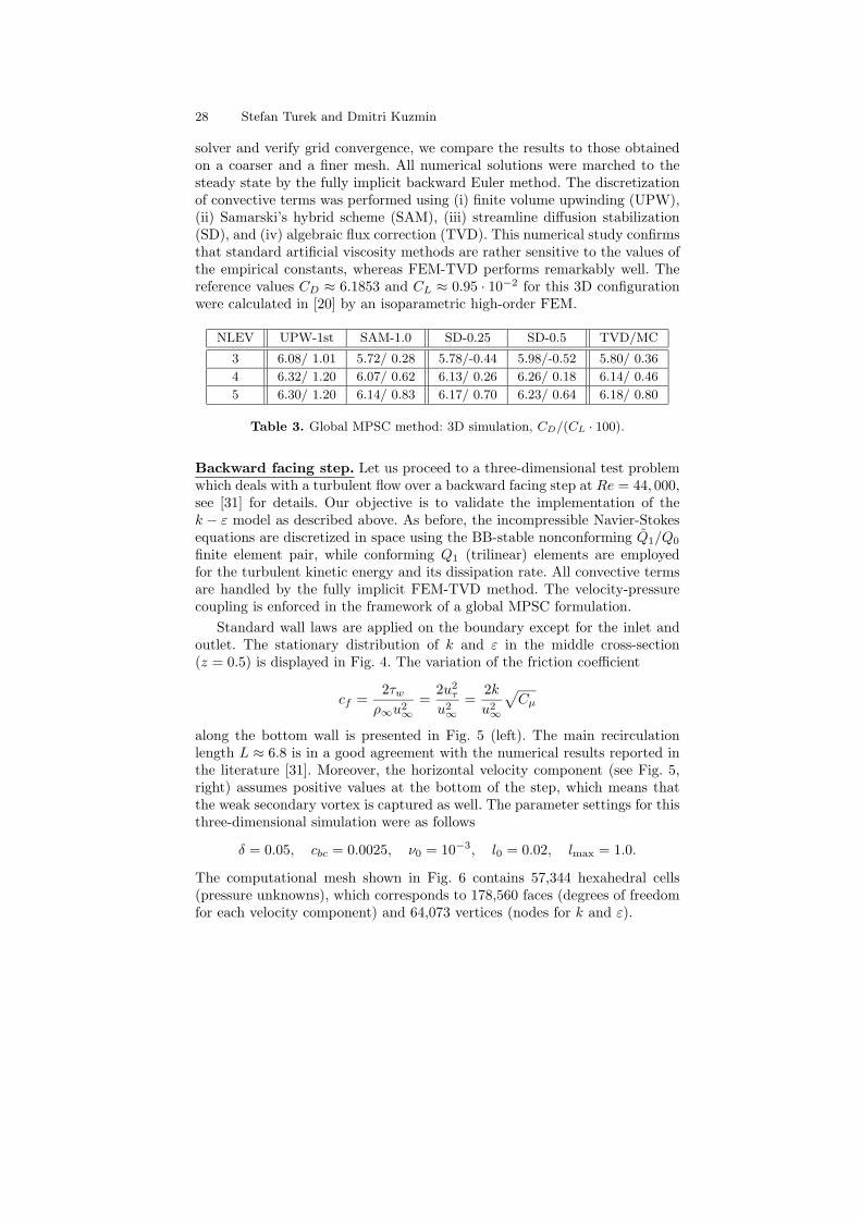
along the bottom wall is presented in Fig. 5 (left). The main recirculationlength L ≈ 6.8 is in a good agreement with the numerical results reported inthe literature [31]. Moreover, the horizontal velocity component (see Fig. 5,right) assumes positive values at the bottom of the step, which means thatthe weak secondary vortex is captured as well. The parameter settings for thisthree-dimensional simulation were as follows
δ = 0.05, cbc = 0.0025, ν0 = 10−3, l0 = 0.02, lmax = 1.0.
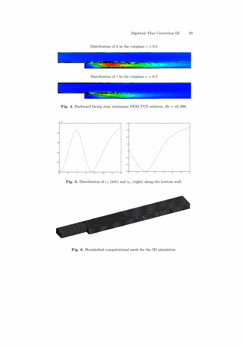
The computational mesh shown in Fig. 6 contains 57,344 hexahedral cells(pressure unknowns), which corresponds to 178,560 faces (degrees of freedomfor each velocity component) and 64,073 vertices (nodes for k and ε).
Algebraic Flux Correction III 29
Distribution of k in the cutplane z = 0.5
Distribution of ε in the cutplane z = 0.5
Fig. 4. Backward facing step: stationary FEM-TVD solution, Re = 44, 000.
0 2 4 6 8 10 12 140
0.2
0.4
0.6
0.8
1x 10
−3
0 2 4 6 8 10 12 14−0.3
−0.2
−0.1
0
0.1
0.2
0.3
0.4
Fig. 5. Distribution of cf (left) and ux (right) along the bottom wall.
Fig. 6. Hexahedral computational mesh for the 3D simulation.
30 Stefan Turek and Dmitri Kuzmin
11 Application to More Complex Flow Models
In this section, we discuss several incompressible flow models which call forthe use of algebraic flux correction (FCT or TVD techniques). Specifically, letus consider generalized Navier-Stokes problems of the form
ρ
(
∂u
∂t+ u · ∇u
)
= f + µ∆u −∇p , ∇ · u = 0 (65)
complemented by additional PDEs which describe physical processes like
1. Heat transfer in complex geometries→ Ceramic plate heat exchanger
2. Multiphase flow with chemical reaction→ Gas-liquid reactors
3. Nonlinear fluids/granular flow→ Sand motion in silos
4. Free and moving boundaries→ Level set FEM methods
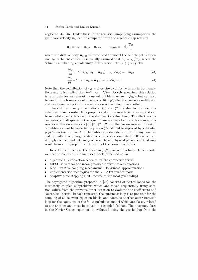
Although these typical flow configurations (to be presented below) differ intheir complexity and cover a wide range of Reynolds numbers, all of themrequire an accurate treatment of convective transport. Numerical artifactssuch as small-scale oscillations/ripples may cause an abnormal termination ofthe simulation run due to division by zero, floating point overflow etc. How-ever, in the worst case they can be misinterpreted as physical phenomena andeventually result in making wrong decisions for the design of industrial equip-ment. Therefore, nonphysical solution behavior should be avoided at any cost,and the use of FEM-FCT/TVD or similar high-resolution schemes is recom-mendable. Moreover, simulation results must be validated by comparison withexperimental data and/or numerical solutions computed on a finer mesh.
11.1 Heat Transfer in ‘Plate Heat Exchangers’
The first example deals with the development of optimization tools for a con-stellation described by ‘coupled stacks’ with different layers (see Fig. 7). Thisexample is quite typical for a complex flow model in the laminar regime. Onthe one hand, the Reynolds number is rather small due to slow fluid veloci-ties and very small diameters. On the other hand, an unstructured grid FEMapproach is required to resolve the small-scale geometrical details. Moreover,the problem at hand is coupled with additional tracer equations of convection-diffusion type. As a rule, the involved diffusion coefficients are small or equalto zero, so that the problem is transport-dominated. Hence, the key elementsof an accurate and efficient solution strategy are an appropriate treatment ofconvective terms on unstructured meshes as well as an unconditionally sta-ble implicit time discretization (the underlying flow field is quasi-stationary).These critical aspects will be exemplarily illustrated in what follows.
Algebraic Flux Correction III 31
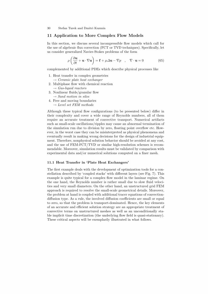
a) b) c)
Fig. 7. Plate heat exchanger: a) geometric configuration; b) typical flow pattern;c) velocity field for an ‘optimal’ distribution of internal objects.
The aim of the underlying numerical study in this section is the under-standing and improvement of the
• internal flow characteristics• heat transfer characteristics
in the shown configuration which can be described by a Boussinesq model.Restricted to one stack only, the internal geometry between ‘inflow’ and ‘out-flow’ holes has to be analyzed and channel-like structures or many internal‘objects’ have to be placed to achieve a homogeneous flow field and, corre-spondingly, a homogeneous distribution of tracer substances in the interior. Inorder to determine the optimal shape and distribution of internal obstacles,the simulation software to be developed must be capable of resolving all small-scale details. Therefore, the underlying numerical algorithm must be highlyaccurate and, moreover, sufficiently flexible and robust. Algebraic FCT/TVDschemes belong to the few discretization techniques that do meet these require-ments. Some preliminary results based on the incompressible Navier-Stokesequations for velocity and pressure only are presented in Fig. 7.
The following step beyond ‘manual optimization’ shall be a fully automaticoptimization of shape, number, and distribution of the internal objects. Fur-thermore, the temperature equations are to be solved for each stack as well asfor the whole system taking into account heat transfer both in the flow fieldand between the walls. In addition, chemical reaction models should be in-cluded, which gives rise to another set of coupled convection-reaction-diffusionequations. Last but not least, algebraic flux correction is to be employed atthe postprocessing step, whereby the ‘residence time distribution’ inside eachstack is measured by solving a pure transport equation for passive tracers.Since the flow field is almost stationary and allows large time steps due to thelarge viscosity parameters, the nonlinear transport equation has to be treatedin an implicit way which is a quite typical requirement for the accurate andefficient treatment for such type of flow problems.
32 Stefan Turek and Dmitri Kuzmin
11.2 Bubbly Flow in Gas-Liquid Reactors
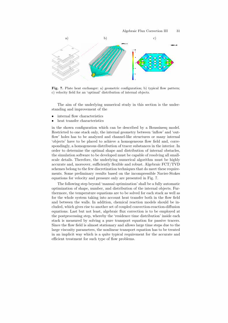
Bubble columns and airlift loop reactors are widely used in industry as con-tacting devices which enable gaseous and liquid species to engage in chemicalreactions. The liquid is supplied continuously or in a batch mode and agitatedby bubbles fed at the bottom of the reactor. As the bubbles rise, the gaseouscomponent is gradually absorbed into the bulk liquid where it may react withother species. The geometric simplicity of bubble columns makes them rathereasy to build, operate and maintain. At the same time, the prevailing flowpatterns are very complex and unpredictable, which represents a major bot-tleneck for the design of industrial units. By insertion of internal parts, bubblecolumns can be transformed into airlift loop reactors which exhibit a stablecirculation pattern with pronounced riser and downcomer zones (see Fig. 8).Hence, shape optimization appears to be a promising way to improve thereactor performance by adjusting the geometry of the internals.
Riser RiserRiserDowncomer Downcomer
Fig. 8. Bubble columns (left) and airlift loop reactors (right).
In the present chapter, we adopt a simplified two-fluid model which isbased on an analog of the Boussinesq approximation (29) for natural convec-tion problems. At moderate gas holdups, the gas-liquid mixture behaves asa weakly compressible fluid which is driven by the bubble-induced buoyancy.Following Sokolichin et al. [44],[45] we assume the velocity uL of the liquidphase to be divergence-free. The dependence of the effective density ρL on thelocal gas holdup ǫ is taken into account only in the gravity force, which is acommon practice for single-phase flows induced by temperature gradients.
Algebraic Flux Correction III 33
This leads to the following generalization of the Navier-Stokes equations
∂uL
∂t+ uL · ∇uL = −∇p∗ + ∇ ·
(
νT [∇uL + ∇uTL]
)
− ǫg,
∇ · uL = 0, p∗ =p − patm
ρL+ g · eg − gh, (66)
where the eddy viscosity νT = Cµk2/ε is a function of the turbulent kineticenergy k and its dissipation rate ε (see above). Recall that the evolution ofthese quantities is described by two scalar transport equations
∂k
∂t+ ∇ ·
(
kuL − νT
σk∇k
)
= Pk + Sk − ε, (67)
∂ε
∂t+ ∇ ·
(
εuL − νT
σε∇ε
)
=ε
k(C1Pk + CεSk − C2ε), (68)
where the extra source terms are due to the bubble-induced turbulence
Pk =νT
2|∇u + ∇uT |2, (69)
Sk = −Ckǫ∇p · uslip. (70)
The involved slip velocity uslip is proportional to the pressure gradient
uslip = − ∇p
CW
and the ‘drag’ coefficient CW ≈ 5 · 104 kgm3s is determined from empirical
correlations for the rise velocity of a single bubble in a stagnant liquid [44].
The gas density ρG is related to the common pressure p by the ideal gaslaw p = ρG
Rη T , which enables us to express the local gas holdup ǫ and the
interfacial area aS per unit volume as follows [26],[28]
ǫ =ρGRT
pη, aS = (4πn)1/3(3ǫ)2/3.
The effective density ρG = ǫρG and the number density n (number of bubblesper unit volume) satisfy the following continuity equations
∂ρG
∂t+ ∇ · (ρGuG) = −mint, (71)
∂n
∂t+ ∇ · (nuG) = 0. (72)
The interphase momentum transfer is typically dominated by the dragforce and the density of gas is much smaller than that of liquid, so that theinertia and gravity terms in the momentum equation for the gas phase can be
34 Stefan Turek and Dmitri Kuzmin
neglected [44],[45]. Under these (quite realistic) simplifying assumptions, thegas phase velocity uG can be computed from the algebraic slip relation
uG = uL + uslip + udrift, udrift = −dG∇n
n,
where the drift velocity udrift is introduced to model the bubble path disper-sion by turbulent eddies. It is usually assumed that dG = νT /σG, where theSchmidt number σG equals unity. Substitution into (71)–(72) yields
∂ρG
∂t+ ∇ · (ρG(uL + uslip) − νT∇ρG) = −mint, (73)
∂n
∂t+ ∇ · (n(uL + uslip) − νT∇n) = 0. (74)
Note that the contribution of udrift gives rise to diffusive terms in both equa-tions and it is implied that ρG∇n/n = ∇ρG. Strictly speaking, this relationis valid only for an (almost) constant bubble mass m = ρG/n but can alsobe used in the framework of ‘operator splitting’, whereby convection-diffusionand reaction-absorption processes are decoupled from one another.
The sink term mint in equations (71) and (73) is due to the reaction-enhanced mass transfer. It is proportional to the interfacial area aS and canbe modeled in accordance with the standard two-film theory. The effective con-centrations of all species in the liquid phase are described by extra convection-reaction-diffusion equations [23],[25],[26],[28]. If the coalescence and breakupof bubbles cannot be neglected, equation (72) should be replaced by a detailedpopulation balance model for the bubble size distribution [11]. In any case, weend up with a very large system of convection-dominated PDEs which arestrongly coupled and extremely sensitive to nonphysical phenomena that mayresult from an improper discretization of the convective terms.
In order to implement the above drift-flux model in a finite element code,we need to collect all the numerical tools presented so far
• algebraic flux correction schemes for the convective terms• MPSC solvers for the incompressible Navier-Stokes equations• block-iterative coupling mechanisms (Boussinesq approximation)• implementation techniques for the k − ε turbulence model• adaptive time-stepping (PID control of the local gas holdup)
The segregated algorithm proposed in [28] consists of nested loops for theintimately coupled subproblems which are solved sequentially using solu-tion values from the previous outer iteration to evaluate the coefficients andsource/sink terms. In each time step, the outermost loop is responsible for thecoupling of all relevant equation blocks and contains another outer iterationloop for the equations of the k− ε turbulence model which are closely relatedto one another and must be solved in a coupled fashion. The buoyancy forcein the Navier-Stokes equations is evaluated using the gas holdup from the
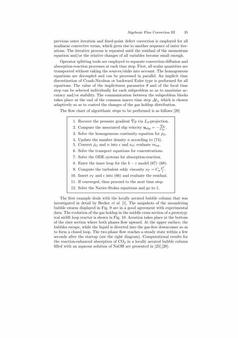
Algebraic Flux Correction III 35
previous outer iteration and fixed-point defect correction is employed for allnonlinear convective terms, which gives rise to another sequence of outer iter-ations. The iterative process is repeated until the residual of the momentumequation and/or the relative changes of all variables become small enough.
Operator splitting tools are employed to separate convection-diffusion andabsorption-reaction processes at each time step. First, all scalar quantities aretransported without taking the sources/sinks into account. The homogeneousequations are decoupled and can be processed in parallel. An implicit timediscretization of Crank-Nicolson or backward Euler type is performed for allequations. The value of the implicitness parameter θ and of the local timestep can be selected individually for each subproblem so as to maximize ac-curacy and/or stability. The communication between the subproblem blockstakes place at the end of the common macro time step ∆tn which is chosenadaptively so as to control the changes of the gas holdup distribution.
The flow chart of algorithmic steps to be performed is as follows [28]
1. Recover the pressure gradient ∇p via L2-projection.
2. Compute the associated slip velocity uslip = − ∇pCW
.
3. Solve the homogeneous continuity equation for ρG.
4. Update the number density n according to (74).5. Convert ρG and n into ǫ and aS ; evaluate mint.
6. Solve the transport equations for concentrations.
7. Solve the ODE systems for absorption-reaction.
8. Enter the inner loop for the k − ε model (67)–(68).
9. Compute the turbulent eddy viscosity νT = Cµk2
ε .
10. Insert νT and ǫ into (66) and evaluate the residual.
11. If converged, then proceed to the next time step.
12. Solve the Navier-Stokes equations and go to 1.
The first example deals with the locally aerated bubble column that wasinvestigated in detail by Becker et al. [1]. The snapshots of the meanderingbubble swarm displayed in Fig. 9 are in a good agreement with experimentaldata. The evolution of the gas holdup in the middle cross section of a prototyp-ical airlift loop reactor is shown in Fig. 10. Aeration takes place at the bottomof the riser section where both phases flow upward. At the upper surface, thebubbles escape, while the liquid is diverted into the gas-free downcomer so asto form a closed loop. The two-phase flow reaches a steady state within a fewseconds after the startup (see the right diagram). Computational results forthe reaction-enhanced absorption of CO2 in a locally aerated bubble columnfilled with an aqueous solution of NaOH are presented in [25],[28].
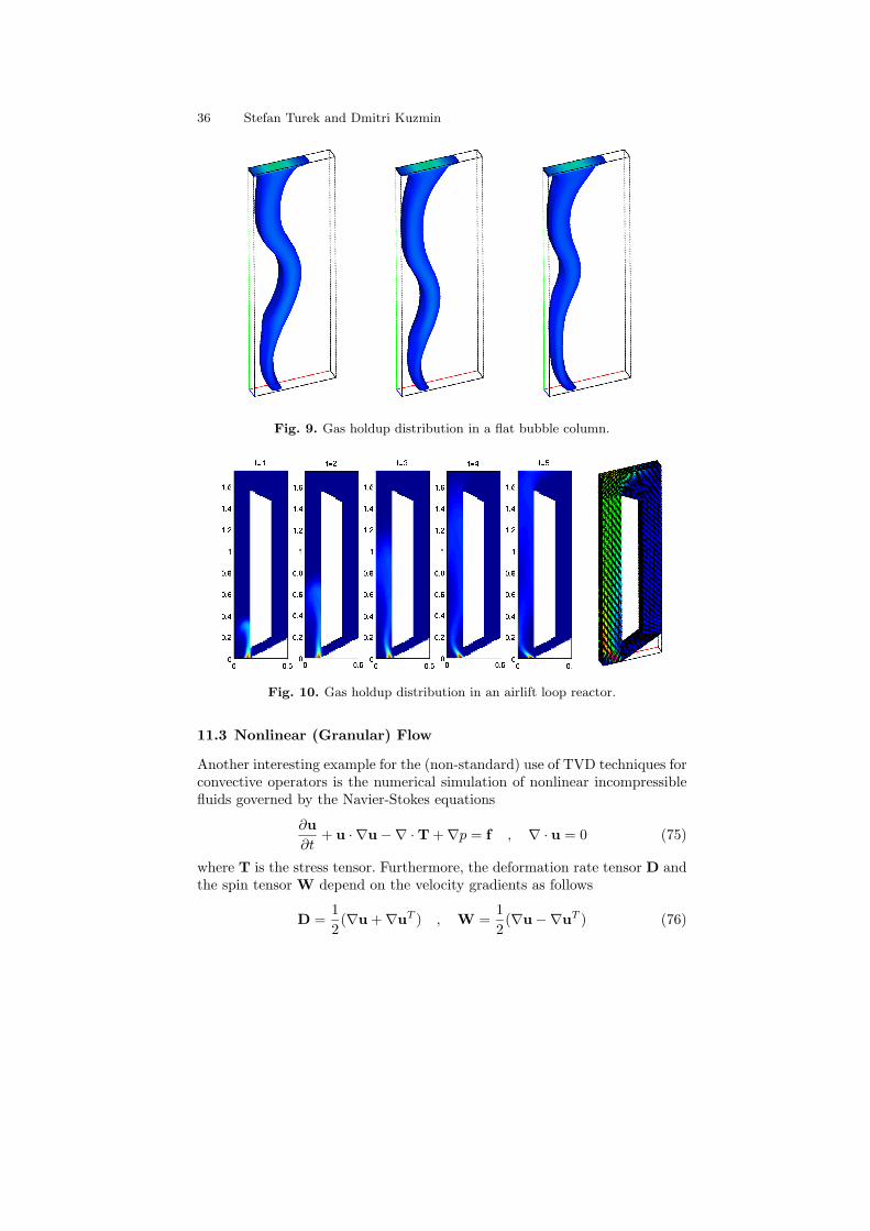
36 Stefan Turek and Dmitri Kuzmin
Fig. 9. Gas holdup distribution in a flat bubble column.
Fig. 10. Gas holdup distribution in an airlift loop reactor.
11.3 Nonlinear (Granular) Flow
Another interesting example for the (non-standard) use of TVD techniques forconvective operators is the numerical simulation of nonlinear incompressiblefluids governed by the Navier-Stokes equations
∂u
∂t+ u · ∇u −∇ · T + ∇p = f , ∇ · u = 0 (75)
where T is the stress tensor. Furthermore, the deformation rate tensor D andthe spin tensor W depend on the velocity gradients as follows
D =1
2(∇u + ∇uT ) , W =
1
2(∇u −∇uT ) (76)
Algebraic Flux Correction III 37
In the case of Newtonian fluids, the stress tensor in (75) is given by
T = 2νD = ν(∇u + ∇uT ). (77)
The most popular representatives of nonlinear fluids are described bypower law models, whereby the viscosity ν in the constitutive relation (77)depends on D = D(u) in a nonlinear way
T = 2ν(D)D , ν(D) = ν0(ǫ1 + ǫ2|D|)α (78)
with certain parameters ν0, ǫ1, ǫ2 and α. Fluids with α > 0 correspond toshear thickening, in contrast to the case α < 0 (shear thinning), both of whichlead to numerical challenges. Such differential type models — see also Binghamor Reiner-Rivlin fluids [30],[38] — do not require implicit calculations of Tsince the tensor T can be represented as a (nonlinear) function of D(u). Onlymodifications of existing Navier-Stokes solvers have to be performed, withoutan additional discretization of equations for T.
This is in contrast to the more general class of rate type models whichcouple (nonlinear) evaluations and derivatives of T with functional evaluationsand derivatives of u and D in space and time. Examples are Rivlin-Ericksenand second grade fluids [21],[30] and particularly Oldroyd models [13],[38].Defining the objective time derivative of the tensor T as
DaT
Dt=
∂T
∂t+ u · ∇T + TW + (TW)T − a[TD + (TD)T ] , (79)
where −1 ≤ a ≤ 1, a general description for Oldroyd models [18],[37] reads
λ1DaT
Dt+ T + γ(T,D) = 2µ
(
λ2DaD
Dt+ D
)
. (80)
The relaxation time λ1, retardation time λ2 and viscosity parameter µ mayadditionally depend on D. In variants with γ(T,D) 6= 0 (Oldroyd 8 constantsmodel, Larson model, Phan-Thien-Tanner model), there is another nonlinearrelationship between T and D, while in the following we will concentrate onthe case γ(T,D) = 0 including the so-called Jeffrey models, resp., the Maxwellfluids. Examples of numerical simulations can be found in papers by Joseph[21], Glowinski [13] and Hron [18]. Consider the following equation for T
T = 2µvD + S , λDaS
Dt+ S = 2µeD, (81)
where λ = λ1, µv = µλ2
λ1
and µe = µ − µv. Then, we can rewrite the Navier-Stokes model in (75) as
Re
[
∂u
∂t+ u · ∇u
]
+ ∇p − (1 − α)∆u −∇ · S = f , ∇ · u = 0 (82)
We
[
∂S
∂t+ u · ∇S + βa(S,D)
]
+ S = 2αD. (83)
38 Stefan Turek and Dmitri Kuzmin
Given −1 ≤ a ≤ 1, let us introduce the following definitions
βa(S,D) = SW + (SW)T − a[SD + (SD)T ] (84)
α =µe
µe + µv, Re =
LVρ
µe + µv, We =
Vλ
L, (85)
where L stands for a characteristic length and V is the velocity.As a result, we end up with a coupled Navier-Stokes-like system (82) for
the variables (u, p) with an additional term ∇·S. Furthermore, there is a non-linear nonstationary tensor-valued transport-reaction equation in (83) whichinvolves both S and D(u). To solve this highly complex system, appropriatediscretization techniques in space and time (implicit Euler, Crank-Nicolson orthe fractional step method in conjunction with BB-stable FEM approxima-tions) should be employed. In particular, the algebraic TVD techniques are tobe recommended for the tensor-valued transport problems since there is an ob-vious need for a monotone, oscillation-free and highly accurate discretizationof the tensor T. Moreover, the above-mentioned MPSC approach to solvingdiscrete saddle point problems and providing a proper coupling between theequations at hand turns out very handy for this kind of applications.
Finally, we mention the hypoplastic model proposed by Kolymbas [22] forthe numerical simulation of dry cohesionless granular materials, for instancefor the flow of sand in silos. This approach contains components from rate typeas well as from differential type models such that the relation to the previouslydescribed Oldroyd model becomes evident:
Re
[
∂u
∂t+ u · ∇u
]
= −∇p + ∇ · T + f , ∇ · u = 0 (86)
∂T
∂t+ (u · ∇)T = − [TW − WT] (87)
+C11
2(TD − DT) + C2tr(TD) · I
+C3
√trD2T + C4
√trD2
trTT2
+ ν(D)
[
∂D
∂t+ u · ∇D + DW − WD
]
.
Here, I denotes the unit matrix, ν(D) a nonlinear (tensorial) function ofpower law type, and Ci are specific material constants. Again, the robust andaccurate treatment of the convective terms in the absence of any second orderelliptic diffusive term is a very important aspect for numerical simulations sothe use of FEM-TVD techniques appears to be especially promising.
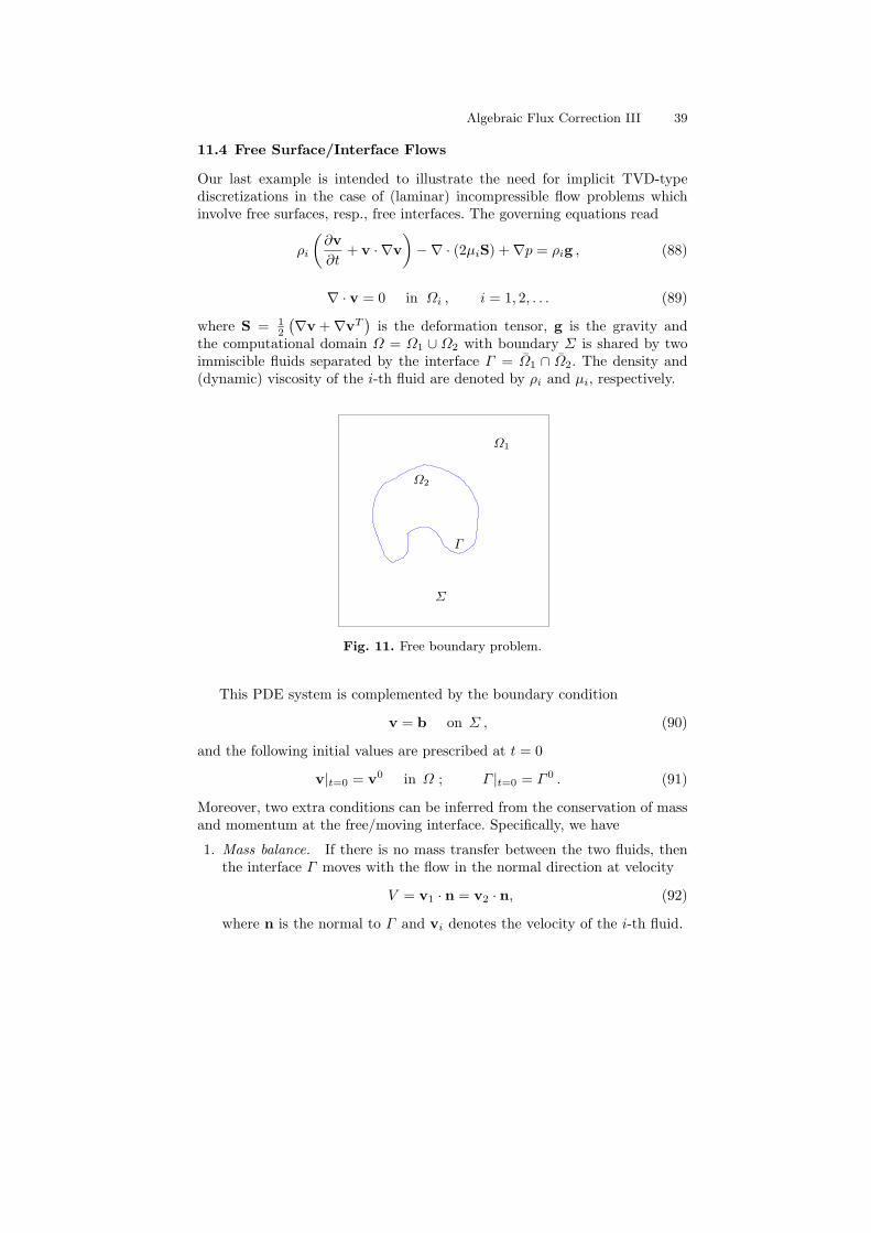
Algebraic Flux Correction III 39
11.4 Free Surface/Interface Flows
Our last example is intended to illustrate the need for implicit TVD-typediscretizations in the case of (laminar) incompressible flow problems whichinvolve free surfaces, resp., free interfaces. The governing equations read
ρi
(
∂v
∂t+ v · ∇v
)
−∇ · (2µiS) + ∇p = ρig , (88)
∇ · v = 0 in Ωi , i = 1, 2, . . . (89)
where S = 12
(
∇v + ∇vT)
is the deformation tensor, g is the gravity andthe computational domain Ω = Ω1 ∪ Ω2 with boundary Σ is shared by twoimmiscible fluids separated by the interface Γ = Ω1 ∩ Ω2. The density and(dynamic) viscosity of the i-th fluid are denoted by ρi and µi, respectively.
Fig. 11. Free boundary problem.
Ω1
Ω2
Γ
Σ
This PDE system is complemented by the boundary condition
v = b on Σ , (90)
and the following initial values are prescribed at t = 0
v|t=0 = v0 in Ω ; Γ |t=0 = Γ 0 . (91)
Moreover, two extra conditions can be inferred from the conservation of massand momentum at the free/moving interface. Specifically, we have
1. Mass balance. If there is no mass transfer between the two fluids, thenthe interface Γ moves with the flow in the normal direction at velocity
V = v1 · n = v2 · n, (92)
where n is the normal to Γ and vi denotes the velocity of the i-th fluid.
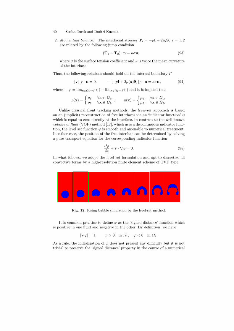
40 Stefan Turek and Dmitri Kuzmin
2. Momentum balance. The interfacial stresses Ti = −pI + 2µiS, i = 1, 2are related by the following jump condition
(T1 − T2) · n = κσn, (93)
where σ is the surface tension coefficient and κ is twice the mean curvatureof the interface.
Thus, the following relations should hold on the internal boundary Γ
[v] |Γ · n = 0 , − [−pI + 2µ(x)S] |Γ · n = κσn , (94)
where [·]|Γ = limx∈Ω2→Γ (·) − limx∈Ω1→Γ (·) and it is implied that
ρ(x) =
ρ1, ∀x ∈ Ω1,ρ2, ∀x ∈ Ω2,
, µ(x) =
µ1, ∀x ∈ Ω1,µ2, ∀x ∈ Ω2.
Unlike classical front tracking methods, the level-set approach is basedon an (implicit) reconstruction of free interfaces via an ‘indicator function’ ϕwhich is equal to zero directly at the interface. In contrast to the well-knownvolume of fluid (VOF) method [17], which uses a discontinuous indicator func-tion, the level set function ϕ is smooth and amenable to numerical treatment.In either case, the position of the free interface can be determined by solvinga pure transport equation for the corresponding indicator function
∂ϕ
∂t+ v · ∇ϕ = 0. (95)
In what follows, we adopt the level set formulation and opt to discretize allconvective terms by a high-resolution finite element scheme of TVD type.
Fig. 12. Rising bubble simulation by the level-set method.
It is common practice to define ϕ as the ‘signed distance’ function whichis positive in one fluid and negative in the other. By definition, we have
|∇ϕ| = 1, ϕ > 0 in Ω1, ϕ < 0 in Ω2.
As a rule, the initialization of ϕ does not present any difficulty but it is nottrivial to preserve the ‘signed distance’ property in the course of a numerical
Algebraic Flux Correction III 41
simulation. Therefore, it is advisable to ‘reinitialize’ ϕ once in a while so asto provide an accurate representation of the free interface.
Given the numerical solution ϕold of the pure transport problem (95) aftera certain number of time steps, we seek a signed distance function ϕ whichhas the same zero level set as ϕold. It can be recovered as the steady-statesolution of another (nonlinear) transport equation which reads
∂ϕ
∂t= sign(ϕold)(1 − |∇ϕ|). (96)
This auxiliary problem for the reinitialization step can be cast in the form
∂ϕ
∂t+ w · ∇ϕ = sign(ϕold), w = sign(ϕold)
∇ϕ
|∇ϕ| (97)
and solved by a suitable pseudo-time-stepping method. In particular, thiscan be accomplished in the framework of an implicit TVD-like discretizationwhich is guaranteed to produce nonoscillatory and highly accurate results.Numerical studies indicate that a proper treatment of the level set function ϕis crucial to the quality of the interface reconstruction so that the convectiveterms in equations (95) and (97) should be handled with extreme care.
12 Conclusions
Even for laminar flow models, there is still a strong need for better mathe-matical approaches as far as the discretization and solution aspects are con-cerned. The accuracy, flexibility, robustness and, particularly, overall efficiencyof many currently available simulation tools leave a lot to be desired. The nextlaborious step is to develop professional CFD software for grand-challengeindustrial problems. However, benchmark computations and other numeri-cal studies demonstrate that one must make every effort to hone and refinethe ‘basic tools’ before proceeding to more complex simulations! Otherwise,there might be no chance to succeed in tackling many challenging applicationsand to achieve not only qualitatively, but also quantitatively accurate results.Hence, the list of topics to be addressed in the near future is as follows:
• Higher order FEM spaces: Preliminary investigations performed byour group and others show that polynomial approximations of higher or-der accuracy might be preferable. Even for the Q2/P1 finite element pair(biquadratic velocity, piecewise linear pressure), the efficiency gains can beenormous. However, it is currently not clear how high-order finite elementswould behave for nonsmooth solutions which exhibit strong gradients. Inparticular, an appropriate stabilization of the convective terms is necessaryat high Reynolds numbers. Algebraic flux correction of FCT/TVD typeseems to be feasible but its extension to the Q2 elements is not obvious.Another primary goal is the development of hierarchical multigrid solvers
42 Stefan Turek and Dmitri Kuzmin
which should ensure that the potential advantages of using higher-orderFEM approximations can be realized in practice.
• Nonlinear solvers: Since TVD-like discretization techniques are per senonlinear, appropriate Newton-like methods are to be applied if an im-plicit treatment of the convective terms is adopted, e.g., for the ‘tracertransport’ in a low Reynolds number flow or at the ‘reinitialization step’for the level set function. However, due to the fully discrete and inherentlydiscontinuous nature of algebraic flux correction schemes, the derivationof the (approximate) Jacobian matrices poses a formidable problem whichis still largely unsolved and calls for further research.
• Multigrid solvers: In a similar vein, the numerical behavior of standard(geometric) multigrid solvers for the resulting linear subproblems has notyet been investigated and requires further in-depth studies.
• Tensor-valued transport operators: As described for nonlinear flu-ids, additional hyperbolic problems with tensor-valued transport operatorsmay need to be dealt with. An extension of our algebraic high-resolutionschemes, which were originally developed for scalar quantities, to such ap-plications should be undertaken in the near future.
• A posteriori error control: Since the proposed flux correction tech-niques are applicable to finite element methods, appropriate a posteriorierror control mechanisms for Galerkin-type discretizations can be incorpo-rated. To be more specific, residual-based error estimation via dual prob-lems for user-specified quantities in the spirit of Rannacher and his col-laborators is to be examined. Its generalization to an unstructured gridFEM equipped with algebraic flux limiters would make it possible to gain‘optimal’ control over the local mesh refinement and/or coarsening.
Apart from all these mathematical challenges, the results of recent compu-tational studies (see [49] for a critical discussion) reveal that memory access,not data processing is costly on modern computers. This is the major reasonwhy traditional numerical approaches for PDEs and their realization as CFDsoftware have massive problems with achieving a significant percentage of thepossible peak performance. On the other hand, the Numerical Linear Algebratools for the solution of sparse linear systems with millions of unknowns canbe significantly improved. This can be accomplished, for instance, by resortingto cache-based implementation techniques and exploiting the local structureof data sets for block-structured grids. Such a hardware-oriented approachmay yield an overall speed-up factor of as much as 10 – 1000 even on a sin-gle processor. In addition, the use of optimal parallelization strategies mayincrease the performance of the code by further orders of magnitude.
To realize these ambitious goals, modern numerical methods and program-ming concepts are to be incorporated into CFD simulation tools. Some of thelatest trends are adaptive meshing and a posteriori error control as well asgeneralized multigrid/domain decomposition solvers. Furthermore, the same
Algebraic Flux Correction III 43
philosophy applies to fully implicit Navier-Stokes solvers of MPSC type whichshould also be optimized so as to shift the distribution of CPU times away fromexpensive memory access tasks (assembly of stiffness matrices, defects andresiduals, modifications of the mesh) toward more arithmetic-intensive com-putational work (iterative solution of linear systems by multigrid or Krylov-space methods). It is obvious that the design and implementation of suchadvanced software concepts is not an easy job. However, the foundations havealready been laid in the framework of the ongoing FEAST project (see [50])aimed at the development of such strategies. Iterative solvers based on theabove-mentioned data structures are already available and prove remarkablyefficient as compared to conventional implementation techniques.
In fact, current technological trends indicate that the demand for high-performance CFD software will continue to increase. Although the develop-ment and optimization of such advanced software products may take a verylong time and consume a lot of resources, this investment is certain to yieldhuge gains in the long run. Indeed, numerical simulation of many ‘real life’problems (e.g., turbulent and/or multiphase flows in complex 3D geometries)is still prohibitively expensive. In order to exploit the available computingpower to the full extent, software engineering aspects must be accompaniedby corresponding efforts in the design of optimal numerical algorithms. More-over, the peculiarities of modern hardware architecture should be taken intoaccount. Otherwise, many ‘nice’ mathematical developments may end up be-ing impractical as long as just a small fraction (less than one percent is notunusual) of the potential peak performance can be achieved in practice.
References
1. S. Becker, A. Sokolichin and G. Eigenberger, Gas-liquid flow in bubble columnsand loop reactors: Part II. Chem. Eng. Sci. 49 (1994) 5747–5762.
2. J. P. Boris, F. F. Grinstein, E. S. Oran und R. J. Kolbe, New insights into LargeEddy Simulation, Fluid Dynamics Research 10, Nr. 4-6, 1992, 199-227.
3. A. J. Chorin, Numerical solution of the Navier–Stokes equations. Math. Comp.22 (1968) 745–762.
4. M. A. Christon, P. M. Gresho, S. B. Sutton, Computational predictability of nat-ural convection flows in enclosures. In: K. J. Bathe (ed) Proc. First MIT Con-ference on Computational Fluid and Solid Mechanics, Elsevier, 2001, 1465-1468,2001.
5. R. Codina and O. Soto, Finite element implementation of two-equation and al-gebraic stress turbulence models for steady incompressible flows. Int. J. Numer.Methods Fluids 30 (1999) no. 3, 309-333.
6. M. Crouzeix and P. A. Raviart, Conforming and non–conforming finite elementmethods for solving the stationary Stokes equations, R.A.I.R.O. R–3 (1973)77–104.
7. J. Donea, S. Giuliani, H. Laval and L. Quartapelle, Finite element solution of theunsteady Navier-Stokes equations by a fractional step method. Comput. Meth.Appl. Mech. Engrg. 30 (1982) 53–73.
44 Stefan Turek and Dmitri Kuzmin
8. M. S. Engelman, V. Haroutunian and I. Hasbani, Segregated finite element al-gorithms for the numerical solution of large–scale incompressible flow problems.Int. J. Numer. Meth. Fluids 17 (1993) 323–348.
9. M. S. Engelman, R. L. Sani and P. M. Gresho, The implementation of normaland/or tangential boundary conditions in finite element codes for incompressiblefluid flow. Int. J. Numer. Meth. Fluids 2 (1982) 225–238.
10. J. H. Ferziger and M. Peric, Computational Methods for Fluid Dynamics.Springer, 1996.
11. C. Fleischer, Detaillierte Modellierung von Gas-Flussigkeits-Reaktoren.Fortschr.-Ber. VDI-Reihe 3, Nr. 691, Dusseldorf: VDI Verlag, 2001.
12. V. Girault and P. A. Raviart, Finite Element Methods for Navier–Stokes Equa-tions, Springer Verlag, Berlin–Heidelberg, 1986.
13. R. Glowinski, T. W. Pan, T. I. Hesla, D. D. Joseph, J. Periaux, A fictitious do-main approach to the direct numerical simulation of incompressible viscous flowpast moving rigid bodies: Application to particulate flow. J. Comput. Phys. 169
(2001) 363–426.14. P. M. Gresho, R. L. Sani and M. S. Engelman, Incompressible Flow and the Fi-
nite Element Method: Advection-Diffusion and Isothermal Laminar Flow. Wiley,1998.
15. P.M. Gresho, On the theory of semi–implicit projection methods for viscousincompressible flow and its implementation via a finite element method thatalso introduces a nearly consistent mass matrix, Part 1: Theory, Part 2: Imple-mentation. Int. J. Numer. Meth. Fluids 11 (1990) 587–659.
16. F. F. Grinstein and C. Fureby, On Monotonically Integrated Large Eddy Simu-lation of Turbulent Flows Based on FCT Algorithms. Chapter 3 in this volume.
17. C.W. Hirt, A.A. Amsden and J.L. Cook, An arbitrary Lagrangian-Euleriancomputing method for all flow speeds. J. Comput. Phys. 14 (1974) 227-253.
18. J. Hron, Numerical simulation of visco-elastic fluids. In: WDS’97, Freiburg, 1997.19. T. J. R. Hughes, L. P. Franca and M. Balestra, A new finite element formula-
tion for computational fluid mechanics: V. Circumventing the Babuska–Brezzicondition: A stable Petrov–Galerkin formulation of the Stokes problem accom-modating equal order interpolation. Comp. Meth. Appl. Mech. Engrg. 59 (1986)85–99.
20. V. John, Higher order finite element methods and multigrid solvers in a bench-mark problem for the 3D Navier-Stokes equations. Int. J. Numer. Meth. Fluids40 (2002) 775–798.
21. D. D. Joseph, R. Glowinski, J. Feng, T. W. Pan, A three-dimensional computa-tion of the force and torque on an ellipsoid settling slowly through a viscoelasticfluid. J. Fluid Mech. 283 (1995) 1-16.
22. D. Kolymbas, An outline of hypoplasticity. Archive of Applied Mechanics 61
(1991) 143-151.23. D. Kuzmin, Numerical simulation of mass transfer and chemical reactions in
gas-liquid flows. In: Proceedings of the 3rd European Conference on NumericalMathematics and Advanced Applications, World Scientific, 2000, 237-244.
24. D. Kuzmin and S. Turek, High-resolution FEM-TVD schemes based on a fullymultidimensional flux limiter. J. Comput. Phys. 198 (2004) 131-158.
25. D. Kuzmin and S. Turek, Efficient numerical techniques for flow simulation inbubble column reactors. In: Preprints of the 5th German-Japanese Symposiumon Bubble Columns , VDI/GVC, 2000, 99-104.
Algebraic Flux Correction III 45
26. D. Kuzmin and S. Turek, Finite element discretization tools for gas-liquid flows.In: M. Sommerfeld (ed.), Bubbly Flows: Analysis, Modelling and Calculation,Springer, 2004, 191-201.
27. D. Kuzmin and S. Turek, Multidimensional FEM-TVD paradigm for convection-dominated flows. Technical report 253, University of Dortmund, 2004. In: Pro-ceedings of the IV European Congress on Computational Methods in AppliedSciences and Engineering (ECCOMAS 2004), Volume II, ISBN 951-39-1869-6.
28. D. Kuzmin and S. Turek, Numerical simulation of turbulent bubbly flows. Tech-nical report 254, University of Dortmund, 2004. To appear in: Proceedings of the3rd International Symposium on Two-Phase Flow Modelling and Experimenta-tion, Pisa, September 22-24, 2004.
29. A. J. Lew, G. C. Buscaglia and P.M. Carrica, A note on the numerical treatmentof the k-epsilon turbulence model. Int. J. Comput. Fluid Dyn. 14 (2001) no. 3,201-209.
30. J. Malek, K. R. Rajagopal, M. Ruzicka, Existence and regularity of solutionsand the stability of the rest state for fluids with shear dependent viscosity.Mathematical Models and Methods in Applied Sciences 5 (1995) 789-812.
31. G. Medic and B. Mohammadi, NSIKE - an incompressible Navier-Stokes solverfor unstructured meshes. INRIA Research Report 3644 (1999).
32. B. Mohammadi, A stable algorithm for the k-epsilon model for compressibleflows. INRIA Research Report 1355 (1990).
33. B. Mohammadi and O. Pironneau, Analysis of the k-epsilon turbulence model.Wiley, 1994.
34. S. V. Patankar, Numerical Heat Transfer and Fluid Flow. McGraw-Hill, 1980.35. A. Prohl, Projection and Quasi-Compressibility Methods for Solving the Incom-
pressible Navier-Stokes Equations. Advances in Numerical Mathematics. B. G.Teubner, Stuttgart, 1997.
36. L. Quartapelle, Numerical Solution of the Incompressible Navier-Stokes Equa-tions. Birkhauser Verlag, Basel, 1993.
37. A. Quarteroni, M. Tuveri, A. Veneziani, Computational vascular fluid dynamics.Comp. Vis. Science 2 (2000) 163-197.
38. K. R. Rajagopal, Mechanics of non-Newtonian fluids. In G. P. Galdi and J. Necas(eds), Recent Developments in Theoretical Fluid Mechanics. Pitman ResearchNotes in Mathematics 291, Longman, 1993, 129-162.
39. R. Rannacher and S. Turek, A simple nonconforming quadrilateral Stokes ele-ment. Numer. Meth. PDEs 8 (1992), no. 2, 97-111.
40. M. Schafer and S. Turek (with support of F. Durst, E. Krause, R. Rannacher),Benchmark computations of laminar flow around cylinder, In E.H. Hirschel (ed.),Flow Simulation with High-Performance Computers II, Vol. 52 von Notes onNumerical Fluid Mechanics, Vieweg, 1996, 547–566.
41. R. Schmachtel, Robuste lineare und nichtlineare Losungsverfahren fur die inkom-pressiblen Navier-Stokes-Gleichungen. PhD thesis, University of Dortmund,2003.
42. P. Schreiber, A new finite element solver for the nonstationary incompressibleNavier–Stokes equations in three dimensions, PhD Thesis, University of Heidel-berg, 1996.
43. P. Schreiber and S. Turek, An efficient finite element solver for the nonstation-ary incompressible Navier–Stokes equations in two and three dimensions, Proc.Workshop Numerical Methods for the Navier–Stokes Equations, Heidelberg, Oct.25–28, 1993, Vieweg.
46 Stefan Turek and Dmitri Kuzmin
44. A. Sokolichin, Mathematische Modellbildung und numerische Simulation vonGas-Flussigkeits-Blasenstromungen. Habilitation thesis, University of Stuttgart,2004.
45. A. Sokolichin, G. Eigenberger and A. Lapin, Simulation of buoyancy drivenbubbly flow: established simplifications and open questions. AIChE Journal 50
(2004) no. 1, 24–45.46. S. Turek, On discrete projection methods for the incompressible Navier-Stokes
equations: An algorithmical approach. Comput. Methods Appl. Mech. Engrg.143 (1997) 271–288.
47. S. Turek, Efficient Solvers for Incompressible Flow Problems: An Algorithmicand Computational Approach, LNCSE 6, Springer, 1999.
48. S. Turek et al., FEATFLOW: finite element software for the incompressibleNavier-Stokes equations. User manual, University of Dortmund, 2000. Availableat http://www.featflow.de.
49. S. Turek, C. Becker and S. Kilian, Hardware-oriented numerics and concepts forPDE software. Special Journal Issue for PDE Software, Elsevier, InternationalConference on Computational Science ICCS’2002, Amsterdam, 2002, FUTURE1095 (2003), 1-23.
50. S. Turek, C. Becker and S. Kilian, Some concepts of the software packageFEAST. In: J. M. Palma, J. Dongarra, V. Hernandes (eds), VECPAR’98 - ThirdInternational Conference for Vector and Parallel Processing, Lecture Notes inComputer Science, Springer, Berlin, 1999.
51. S. Turek and S. Kilian, An example for parallel ScaRC and its application to theincompressible Navier-Stokes equations, Proc. ENUMATH’97, World SciencePubl., 1998.
52. S. Turek and R. Schmachtel, Fully coupled and operator-splitting approachesfor natural convection. Int. Numer. Meth. Fluids 40 (2002) 1109-1119.
53. A. M. P. Valli, G. F. Carey and A. L. G. A. Coutinho, Finite element simulationand control of nonlinear flow and reactive transport. In: Proceedings of the 10thInternational Conference on Numerical Methods in Fluids. Tucson, Arizona,1998: 450-45.
54. A. M. P. Valli, G. F. Carey and A. L. G. A. Coutinho, Control strategies fortimestep selection in simulation of coupled viscous flow and heat transfer. Com-mun. Numer. Methods Eng. 18 (2002), no.2, 131-139.
55. S. P. Vanka, Implicit multigrid solutions of Navier–Stokes equations in primitivevariables. J. Comp. Phys. 65 (1985) 138–158.
56. J. Van Kan, A second–order accurate pressure–correction scheme for viscousincompressible flow. SIAM J. Sci. Stat. Comp. 7 (1986) 870–891.