Analysis of numerical dissipation and dispersion

Modified equation method: the exact solution of the discretized equations

satisfies a PDE which is generally different from the one to be solved

Original PDE Modified equation Aun+1 = Bun

∂u

∂t+ Lu = 0 ≈

∂u

∂t+ Lu =

∞∑

p=1

α2p∂2pu

∂x2p+

∞∑

p=1

α2p+1∂2p+1u

∂x2p+1

Motivation: PDEs are difficult or impossible to solve analytically but their

qualitative behavior is easier to predict than that of discretized equations

• Expand all nodal values in the difference scheme in a double Taylor series

about a single point (xi, tn) of the space-time mesh to obtain a PDE

• Express high-order time derivatives as well as mixed derivatives in terms

of space derivatives using this PDE to transform it into the desired form

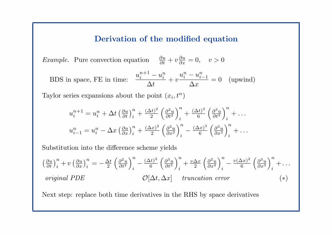
Derivation of the modified equation

Example. Pure convection equation ∂u∂t + v ∂u

∂x = 0, v > 0

BDS in space, FE in time:un+1

i − uni

∆t+ v

uni − un

i−1

∆x= 0 (upwind)

Taylor series expansions about the point (xi, tn)

un+1i = un

i + ∆t(

∂u∂t

)n

i+ (∆t)2

2

(∂2u∂t2

)n

i+ (∆t)3

6

(∂3u∂t3

)n

i+ . . .

uni−1 = un

i −∆x(

∂u∂x

)n

i+ (∆x)2

2

(∂2u∂x2

)n

i− (∆x)3

6

(∂3u∂x3

)n

i+ . . .

Substitution into the difference scheme yields

(∂u∂t

)n

i+ v

(∂u∂x

)n

i= −∆t

2

(∂2u∂t2

)n

i− (∆t)2

6

(∂3u∂t3

)n

i+ v∆x

2

(∂2u∂x2

)n

i− v(∆x)2

6

(∂3u∂x3

)n

i+ . . .

original PDE O[∆t,∆x] truncation error (∗)

Next step: replace both time derivatives in the RHS by space derivatives

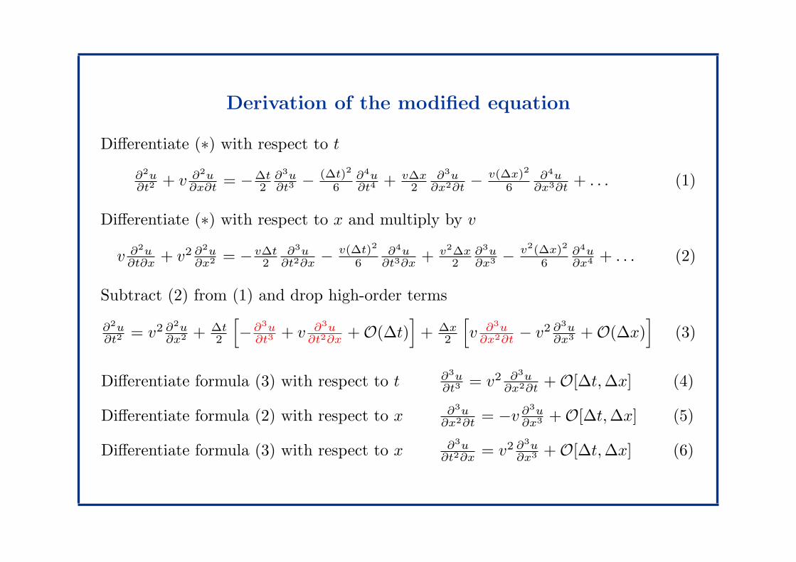
Derivation of the modified equation

Differentiate (∗) with respect to t

∂2u∂t2 + v ∂2u

∂x∂t = −∆t2

∂3u∂t3 −

(∆t)2

6∂4u∂t4 + v∆x

2∂3u

∂x2∂t −v(∆x)2

6∂4u

∂x3∂t + . . . (1)

Differentiate (∗) with respect to x and multiply by v

v ∂2u∂t∂x + v2 ∂2u

∂x2 = − v∆t2

∂3u∂t2∂x −

v(∆t)2

6∂4u

∂t3∂x + v2∆x2

∂3u∂x3 −

v2(∆x)2

6∂4u∂x4 + . . . (2)

Subtract (2) from (1) and drop high-order terms

∂2u∂t2 = v2 ∂2u

∂x2 + ∆t2

[

−∂3u∂t3 + v ∂3u

∂t2∂x +O(∆t)]

+ ∆x2

[

v ∂3u∂x2∂t − v2 ∂3u

∂x3 +O(∆x)]

(3)

Differentiate formula (3) with respect to t ∂3u∂t3 = v2 ∂3u

∂x2∂t +O[∆t,∆x] (4)

Differentiate formula (2) with respect to x ∂3u∂x2∂t = −v ∂3u

∂x3 +O[∆t,∆x] (5)

Differentiate formula (3) with respect to x ∂3u∂t2∂x = v2 ∂3u

∂x3 +O[∆t,∆x] (6)

Derivation of the modified equation

Equations (4) and (5) imply that ∂3u∂t3 = −v3 ∂3u

∂x3 +O[∆t,∆x] (7)

Plug (5)–(7) into (3) ⇒ ∂2u∂t2 = v2 ∂2u

∂x2 + v2(v∆t−∆x)∂3u∂x3 +O[∆t,∆x] (8)

Substitute (7) and (8) into (∗) to obtain the modified equation

∂u∂t + v ∂u

∂x = − v2∆t2

[∂2u∂x2 + (v∆t−∆x)∂3u

∂x3

]

+ v3(∆t)2

6∂3u∂x3 + v∆x

2∂2u∂x2 −

v(∆x)2

6∂3u∂x3 + . . .

which can be rewritten in terms of the Courant number ν = v ∆t∆x as follows

∂u

∂t+ v

∂u

∂x=

v∆x

2(1− ν)

∂2u

∂x2︸ ︷︷ ︸

numerical diffusion

+v(∆x)2

6(3ν − 2ν2 − 1)

∂3u

∂x3︸ ︷︷ ︸

numerical dispersion

+ . . .

Remark. The CFL stability condition ν ≤ 1 must be satisfied for the discrete

problem to be well-posed. In the case ν > 1, the numerical diffusion coefficientv∆x

2 (1− ν) is negative, which corresponds to a backward heat equation

Significance of terms in the modified equation

Exact solution of the discretized equations

Aun+1 = Bun ←→∂u

∂t+ Lu =

∞∑

p=1

α2p∂2pu

∂x2p+

∞∑

p=1

α2p+1∂2p+1u

∂x2p+1

Even-order derivatives ∂2pu∂x2p

cause numerical dissipation

0 0.1 0.2 0.3 0.4 0.5 0.6 0.7 0.8 0.9 1

0

0.2

0.4

0.6

0.8

1

smearing (amplitude errors)

Odd-order derivatives ∂2p+1u∂x2p+1

cause numerical dispersion

0 0.1 0.2 0.3 0.4 0.5 0.6 0.7 0.8 0.9 1

0

0.2

0.4

0.6

0.8

1

wiggles (phase errors)

∂u∂t + v ∂u

∂x = 0

Qualitative analysis: the numerical behavior of the discretization scheme largely

depends on the relative importance of dispersive and dissipative effects

Stabilization by means of artificial diffusion

Stability condition (necessary but not sufficient)

The coefficients of the even-order derivatives in the modified equation must

have alternating signs, the one for the second-order term being positive

If this condition is violated, it can be enforced by adding artificial diffusion:

Stabilized methods +δ(v · ∇)2u streamline diffusion

Nonoscillatory methods +δ(v · ∇)2u + ǫ(u)∆u shock-capturing viscosity

Remark. In the one-dimensional case both terms are proportional to ∂2u∂x2

Free parameters δ = cδh1+|v| , ǫ(u) = cǫh

2R(u)where h is the mesh size

and R(u) is the residual

Problem: how to determine proper values of the constants cδ and cǫ ???

Alternative: use a high-order time-stepping method or flux/slope limiters

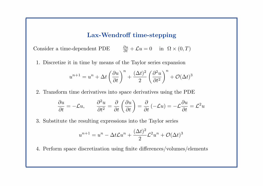
Lax-Wendroff time-stepping

Consider a time-dependent PDE ∂u∂t + Lu = 0 in Ω× (0, T )

1. Discretize it in time by means of the Taylor series expansion

un+1 = un + ∆t

(∂u

∂t

)n

+(∆t)2

2

(∂2u

∂t2

)n

+O(∆t)3

2. Transform time derivatives into space derivatives using the PDE

∂u

∂t= −Lu,

∂2u

∂t2=

∂

∂t

(∂u

∂t

)

=∂

∂t(−Lu) = −L

∂u

∂t= L2u

3. Substitute the resulting expressions into the Taylor series

un+1 = un −∆tLun +(∆t)2

2L2un +O(∆t)3

4. Perform space discretization using finite differences/volumes/elements

Lax-Wendroff scheme for pure convection

Example. Pure convection equation ∂u∂t + v ∂u

∂x = 0 (1D case)

Time derivatives L = v ∂∂x ⇒ ∂u

∂t = −v ∂u∂x , ∂2u

∂t2 = v2 ∂2u∂x2

Semi-discrete scheme un+1 = un − v∆t(

∂u∂x

)n+ (v∆t)2

2

(∂2u∂x2

)n

+O(∆t)3

Central difference approximation in space

(∂u∂x

)

i= ui+1−ui−1

2∆x +O(∆x)2,(

∂2u∂x2

)

i= ui+1−2ui+ui−1

(∆x)2 +O(∆x)2

Fully discrete scheme (second order in space and time)

un+1i − un

i

∆t+ v

uni+1 − un

i−1

2∆x=

v2∆t

2

uni+1 − 2un

i + uni−1

(∆x)2+O[(∆t)2, (∆x)2]

Remark. LW/CDS is equivalent to FE/CDS stabilized by numerical dissipation

due to the second-order term in the Taylor series (no adjustable parameter)

Forward Euler vs. Lax-Wendroff (CDS)

Modified equation for the FE/CDS scheme

∂u∂t + v ∂u

∂x = − v∆x2 ν ∂2u

∂x2 −v(∆x)2

6 (1 + 2ν2)∂3u∂x3 + . . . where ν = v ∆t

∆x

• unconditionally unstable since the coefficient − v∆x2 ν = − v2∆t

2 is negative

Modified equation for the LW/CDS scheme

∂u∂t +v ∂u

∂x = − v(∆x)2

6 (1−ν2)∂3u∂x3−

v(∆x)3

8 ν(1−ν2)∂4u∂x4−

v(∆x)4

120 (1+5ν2−6ν4)∂5u∂x5 +. . .

• conditionally stable for ν2 ≤ 1 in 1D, ν2 ≤ 18 in 2D, ν2 ≤ 1

27 in 3D

• the second-order derivative (leading dissipation error) has been eliminated

• the negative dispersion coefficient corresponds to a lagging phase error i. e.

• harmonics travel too slow, spurious oscillations occur behind steep fronts

• the leading truncation error vanishes for ν2 = 1 (unit CFL property)

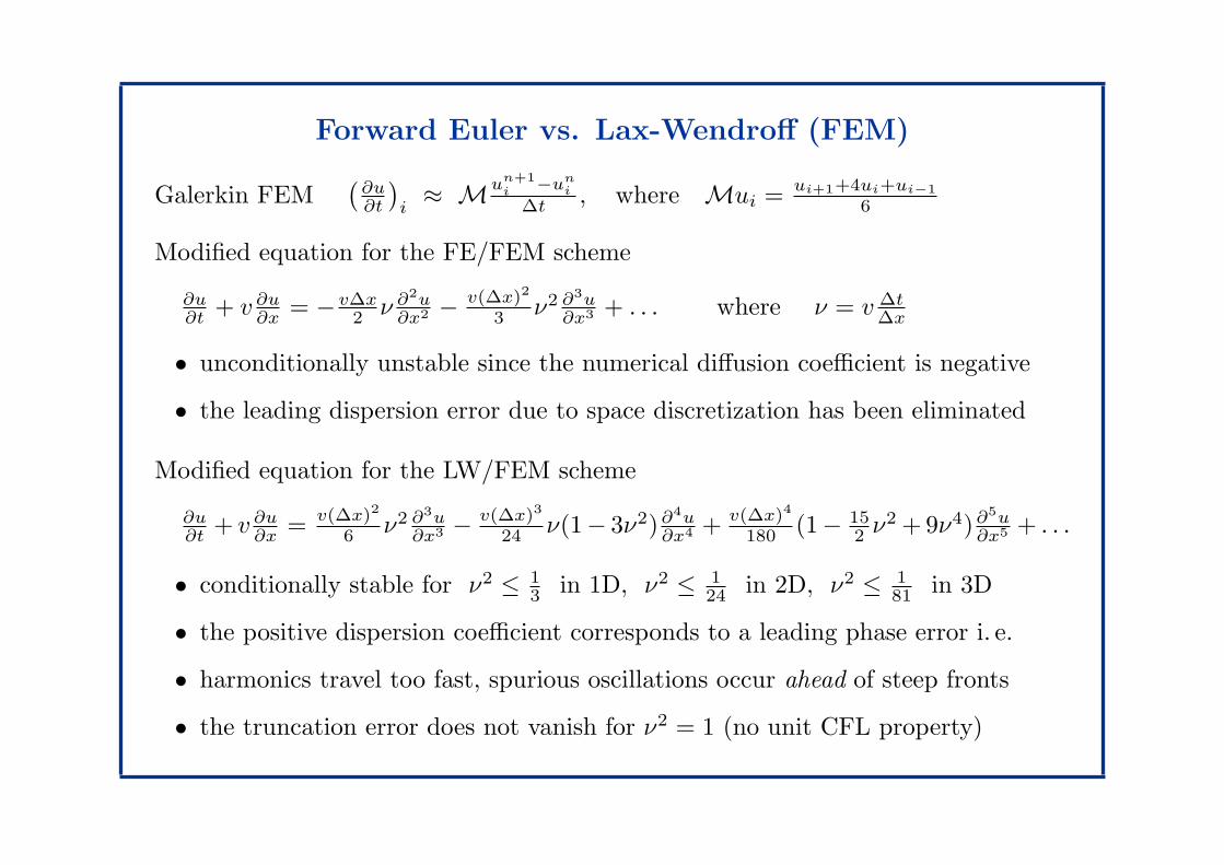
Forward Euler vs. Lax-Wendroff (FEM)

Galerkin FEM(

∂u∂t

)

i≈ M

un+1

i −uni

∆t , where Mui = ui+1+4ui+ui−1

6

Modified equation for the FE/FEM scheme

∂u∂t + v ∂u

∂x = − v∆x2 ν ∂2u

∂x2 −v(∆x)2

3 ν2 ∂3u∂x3 + . . . where ν = v ∆t

∆x

• unconditionally unstable since the numerical diffusion coefficient is negative

• the leading dispersion error due to space discretization has been eliminated

Modified equation for the LW/FEM scheme

∂u∂t + v ∂u

∂x = v(∆x)2

6 ν2 ∂3u∂x3 −

v(∆x)3

24 ν(1− 3ν2)∂4u∂x4 + v(∆x)4

180 (1− 152 ν2 + 9ν4)∂5u

∂x5 + . . .

• conditionally stable for ν2 ≤ 13 in 1D, ν2 ≤ 1

24 in 2D, ν2 ≤ 181 in 3D

• the positive dispersion coefficient corresponds to a leading phase error i. e.

• harmonics travel too fast, spurious oscillations occur ahead of steep fronts

• the truncation error does not vanish for ν2 = 1 (no unit CFL property)

Lax-Wendroff FEM in multidimensions

Pure convection equation ∂u∂t + v · ∇u = 0 in Ω× (0, T ) v = v(x)

Boundary conditions u = g on Γin = x ∈ Γ : v · n < 0 inflow boundary

Time derivatives L = v · ∇ ⇒ ∂u∂t = −v · ∇u streamline derivative

∂2u∂t2 = (v · ∇)2u streamline diffusion (second derivative in the flow direction)

Semi-discrete scheme un+1 = un −∆tv · ∇un + (∆t)2

2 (v · ∇)2un +O(∆t)3

Weak formulation for the Galerkin method∫

Ω

w(un+1 − un) dx = −∆t

∫

Ω

w v · ∇un dx +(∆t)2

2

∫

Ω

w(v · ∇)2un dx

Integration by parts using the identity ∇ · (ab) = a∇ · b + b · ∇a yields

∫

Ωwv · ∇v · ∇u dx = −

∫

Ω∇ · (wv) v · ∇u dx +

∫

Γoutwv · n v · ∇u ds

= −∫

Ωv · ∇w v · ∇u dx−

∫

Ωw∇ · v v · ∇u dx +

∫

Γoutwv · n v · ∇u ds

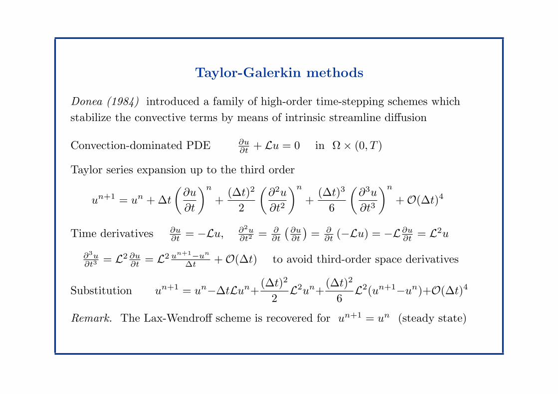
Taylor-Galerkin methods

Donea (1984) introduced a family of high-order time-stepping schemes which

stabilize the convective terms by means of intrinsic streamline diffusion

Convection-dominated PDE ∂u∂t + Lu = 0 in Ω× (0, T )

Taylor series expansion up to the third order

un+1 = un + ∆t

(∂u

∂t

)n

+(∆t)2

2

(∂2u

∂t2

)n

+(∆t)3

6

(∂3u

∂t3

)n

+O(∆t)4

Time derivatives ∂u∂t = −Lu, ∂2u

∂t2 = ∂∂t

(∂u∂t

)= ∂

∂t (−Lu) = −L∂u∂t = L2u

∂3u∂t3 = L2 ∂u

∂t = L2 un+1−un

∆t +O(∆t) to avoid third-order space derivatives

Substitution un+1 = un−∆tLun+(∆t)2

2L2un+

(∆t)2

6L2(un+1−un)+O(∆t)4

Remark. The Lax-Wendroff scheme is recovered for un+1 = un (steady state)

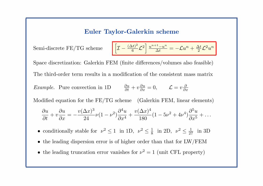
Euler Taylor-Galerkin scheme

Semi-discrete FE/TG scheme[

I − (∆t)2

6 L2]

un+1−un

∆t = −Lun + ∆t2 L

2un

Space discretization: Galerkin FEM (finite differences/volumes also feasible)

The third-order term results in a modification of the consistent mass matrix

Example. Pure convection in 1D ∂u∂t + v ∂u

∂x = 0, L = v ∂∂x

Modified equation for the FE/TG scheme (Galerkin FEM, linear elements)

∂u

∂t+ v

∂u

∂x= −

v(∆x)3

24ν(1− ν2)

∂4u

∂x4+

v(∆x)4

180(1− 5ν2 + 4ν4)

∂5u

∂x5+ . . .

• conditionally stable for ν2 ≤ 1 in 1D, ν2 ≤ 18 in 2D, ν2 ≤ 1

27 in 3D

• the leading dispersion error is of higher order than that for LW/FEM

• the leading truncation error vanishes for ν2 = 1 (unit CFL property)

Leapfrog Taylor-Galerkin scheme

Taylor series un±1 = un ±∆t(

∂u∂t

)n+ (∆t)2

2

(∂2u∂t2

)n

± (∆t)3

6

(∂3u∂t3

)n

+O(∆t)4

It follows that un+1 − un−1 = 2∆t(

∂u∂t

)n+ (∆t)3

3

(∂3u∂t3

)n

+O(∆t)4

Time derivatives ∂u∂t = −Lu, ∂3u

∂t3 = L2 ∂u∂t = L2 un+1−un

∆t +O(∆t)

Semi-discrete LF/TG scheme[

I − (∆t)2

6 L2]

un+1−un−1

2∆t = −Lun

Modified equations for leapfrog schemes with L = v ∂∂x

LF/CDS ∂u∂t + v ∂u

∂x = − v(∆x)2

6 (1− ν2)∂3u∂x3 + v(∆x)4

120 (1− 10ν2 + 9ν4)∂5u∂x5 + . . .

LF/FEM ∂u∂t + v ∂u

∂x = v(∆x)2

6 ν2 ∂3u∂x3 + v(∆x)4

360 (2− 27ν4)∂5u∂x5 + . . .

LF/TG ∂u∂t + v ∂u

∂x = v(∆x)4

360 (2 + 5ν2 − 7ν4)∂5u∂x5 + . . .

• fourth-order accurate, non-dissipative and conditionally stable for ν2 ≤ 1

• the truncation error shrinks as compared to that for 2nd-order LF schemes

• the unit CFL property is satisfied for phase angles in the range 0 ≤ θ ≤ π2

Crank-Nicolson Taylor-Galerkin scheme

Taylor series expansions up to the fourth order

un+1 = un + ∆t(

∂u∂t

)n+ (∆t)2

2

(∂2u∂t2

)n

+ (∆t)3

6

(∂3u∂t3

)n

+O(∆t)4

un = un+1 −∆t(

∂u∂t

)n+1+ (∆t)2

2

(∂2u∂t2

)n+1

− (∆t)3

6

(∂3u∂t3

)n+1

+O(∆t)4

It follows that un+1 = un + ∆t2

[(∂u∂t

)n+

(∂u∂t

)n+1]

+ (∆t)2

4

[(∂2u∂t2

)n

−(

∂2u∂t2

)n+1]

+ (∆t)3

12

[(∂3u∂t3

)n

+(

∂3u∂t3

)n+1]

+O(∆t)4

Time derivatives ∂u∂t = −Lu, ∂2u

∂t2 = ∂∂t

(∂u∂t

)= ∂

∂t (−Lu) = −L∂u∂t = L2u

(∂3u∂t3

)n

+(

∂3u∂t3

)n+1

= L2[(

∂u∂t

)n+

(∂u∂t

)n+1]

= 2L2 un+1−un

∆t +O(∆t)

Fourth-order accurate Crank-Nicolson time-stepping

un+1 = un − ∆t2 L(un + un+1) + (∆t)2

4 L2(un − un+1) + (∆t)2

6 L2(un+1 − un)

Crank-Nicolson Taylor-Galerkin scheme

Semi-discrete CN/TG scheme[

I + ∆t2 L+ (∆t)2

12 L2]

un+1−un

∆t = −Lun

Modified equations for Crank-Nicolson schemes with L = v ∂∂x

CN/CDS ∂u∂t + v ∂u

∂x = − v(∆x)2

6

(

1 + ν2

2

)∂3u∂x3 + v(∆x)4

120 (1 + 5ν2 + 32ν4)∂5u

∂x5 + . . .

CN/FEM ∂u∂t + v ∂u

∂x = − v(∆x)2

12 ν2 ∂3u∂x3 + . . .

CN/TG ∂u∂t + v ∂u

∂x = v(∆x)4

720 (4− 5ν2 + ν4)∂5u∂x5 + . . .

• fourth-order accurate, non-dissipative and unconditionally stable

• cannot be operated at ν2 > 1 since the matrix becomes singular

• the phase response is far superior to that for 2nd-order CN schemes

• the leading truncation error vanishes for ν2 = 1 (unit CFL property)

Remark. Both LF/TG and CN/TG degenerate into the unstable Galerkin

discretization if the solution reaches a steady state so that un+1 = un

Multistep Taylor-Galerkin schemes

Fractional step algorithms of predictor-corrector type lend themselves to the

treatment of (nonlinear) problems described by PDEs of complex structure

Purpose: to avoid a repeated application of spatial differential operators to

the governing equation and/or enhance the accuracy of time discretization

Taylor series un+1 = un + ∆t(

∂u∂t

)n+ (∆t)2

2

(∂2u∂t2

)n

+O(∆t)3

Factorization I + ∆t ∂∂t + (∆t)2

2∂2

∂t2 = I + ∆t ∂∂t

[I + ∆t

2∂∂t

]

Richtmyer scheme (two-step Lax-Wendroff method)

un+1/2 = un + ∆t2

(∂u∂t

)n

un+1 = un + ∆t(

∂u∂t

)n+1/2⇒

un+1/2 = un − ∆t2 Lun

un+1 = un −∆tLun+1/2

• second-order RK method (forward Euler predictor + midpoint rule corrector)

• stability and phase characteristics as for the single-step Lax-Wendroff scheme

Multistep Taylor-Galerkin schemes

Taylor series un+1 = un + ∆t(

∂u∂t

)n+ (∆t)2

2

(∂2u∂t2

)n

+ (∆t)3

6

(∂3u∂t3

)n

+O(∆t)4

Factorization I + ∆t ∂∂t + (∆t)2

2∂2

∂t2 + (∆t)3

6∂3

∂t3 = I + ∆t ∂∂t

[

I + ∆t2

∂∂t + (∆t)2

6∂2

∂t2

]

= I + ∆t ∂∂t

[I + ∆t

2∂∂t

(I + ∆t

3∂∂t

)]no high-order derivatives

Three-step Taylor-Galerkin method (Jiang and Kawahara, 1993)

un+1/3 = un + ∆t3

(∂u∂t

)n

un+1/2 = un + ∆t2

(∂u∂t

)n+1/3

un+1 = un + ∆t(

∂u∂t

)n+1/2

⇒

un+1/3 = un − ∆t3 Lun

un+1/2 = un − ∆t2 Lun+1/3

un+1 = un −∆tLun+1/2

• third-order time-stepping method, conditionally stable for ν2 ≤ 1 (optimal)

• no improvement in phase accuracy as compared to the two-step TG algorithm

• lagging phase error at intermediate and short wavelengths, unit CFL property

High-order Taylor-Galerkin schemes

Multistep TG methods involving second time derivatives offer high accuracy

and an isotropic stability domain for nonlinear multidimensional problems

Two-step third-order TG scheme (Selmin, 1987)

un+1/2 = un + ∆t3

(∂u∂t

)n+ α(∆t)2

(∂2u∂t2

)n

predictor

un+1 = un + ∆t(

∂u∂t

)n+ (∆t)2

2

(∂2u∂t2

)n+1/2

corrector

• α is chosen so as to obtain the desired stability/accuracy characteristics

• excellent phase response of the FE/TG method is reproduced for α = 19

• stable for ν2 ≤ 34 in 1D/2D/3D (no loss of stability in multidimensions)

Underlying factorization vs. Taylor series expansion

I+∆t ∂

∂t+ (∆t)2

2∂2

∂t2

h

I + ∆t

3∂

∂t+ α(∆t)2 ∂

2

∂t2

i

= I+∆t ∂

∂t+ (∆t)2

2∂2

∂t2+ (∆t)3

6∂3

∂t3+α

(∆t)4

2∂4

∂t4

Remark. A fourth-order accurate time-stepping method is recovered for α = 112

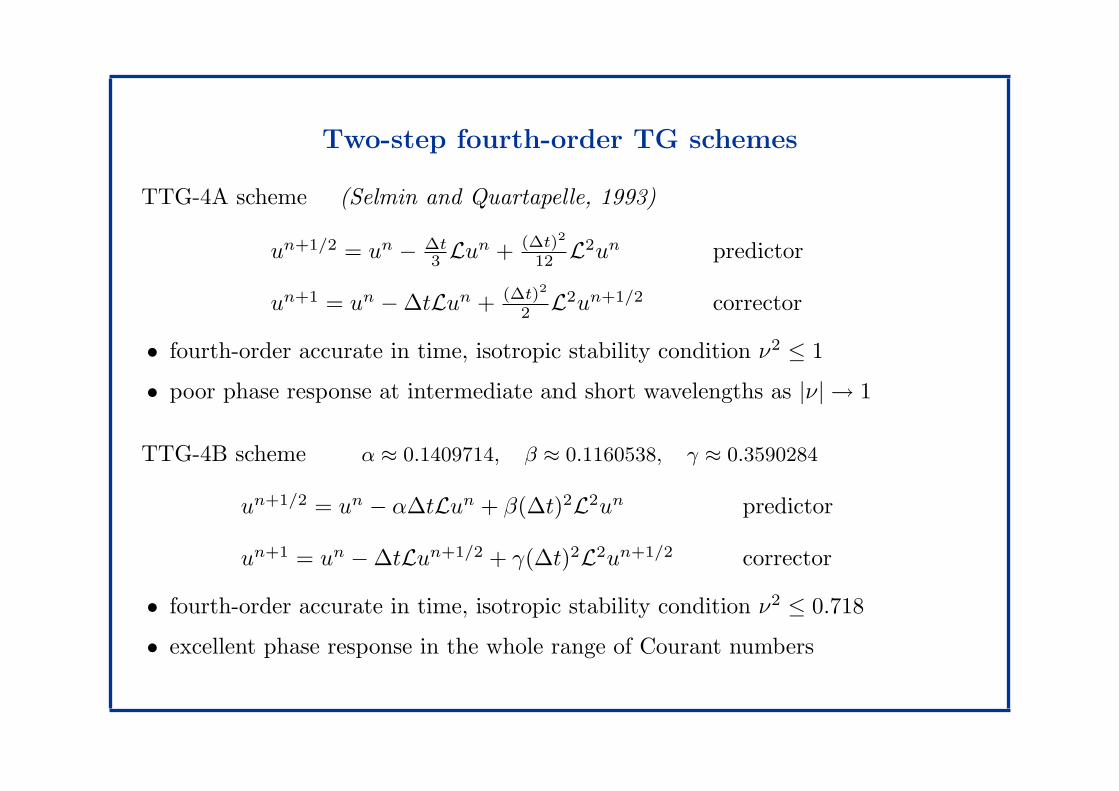
Two-step fourth-order TG schemes

TTG-4A scheme (Selmin and Quartapelle, 1993)

un+1/2 = un − ∆t3 Lun + (∆t)2

12 L2un predictor

un+1 = un −∆tLun + (∆t)2

2 L2un+1/2 corrector

• fourth-order accurate in time, isotropic stability condition ν2 ≤ 1

• poor phase response at intermediate and short wavelengths as |ν| → 1

TTG-4B scheme α ≈ 0.1409714, β ≈ 0.1160538, γ ≈ 0.3590284

un+1/2 = un − α∆tLun + β(∆t)2L2un predictor

un+1 = un −∆tLun+1/2 + γ(∆t)2L2un+1/2 corrector

• fourth-order accurate in time, isotropic stability condition ν2 ≤ 0.718

• excellent phase response in the whole range of Courant numbers

Semi-implicit Taylor-Galerkin schemes

Problem: fully explicit schemes are doomed to be conditionally stable

Semi-implicit Lax-Wendroff method (Hassan et al., 1989)

un+1 = un −∆tLun +(∆t)2

2L2un+1 +O(∆t)3 unconditionally stable

High-order multistep TG schemes (Safjan and Oden, 1993)

[I − λ(∆t)2L2]un+αi = un +

i−1∑

j=0

[−µij∆tL+ νij(∆t)2L2]un+αj , i = 1, . . . , s

Here 0 = α0 ≤ . . . ≤ αs = 1, the free parameter λ is to be chosen from stability

considerations and the coefficients αi, µij , νij must satisfy the order conditions

αki − k

s∑

j=1

[µijαk−1j + νij(k − 1)αk−2

j ] =

µi0, i = 1

2νi0, i = 2

0, otherwise

i = 1, . . . , s

k = 1, . . . , p

for an s-step scheme to be of p−th order (p = 2s is the highest possible accuracy)

Pade approximations

Taylor series expansion (Donea et al., 1998)

un+1 =

[

1 + ∆t∂

∂t+

(∆t)2

2

∂2

∂t2+

(∆t)3

6

∂3

∂t3+ . . .

]

un = exp

(

∆t∂

∂t

)

un

Pade approximations of order p = m + n to the exponential of x = ∆t ∂∂t

Rn,m(x) :=Pn(x)

Qm(x)≈ exp(x) multistage Taylor-Galerkin methods

Example. R2,0 = 1 + x + x2

2 (second order)

un+1 =(1 + x

(1 + x

2

))un = un + ∆t

(∂u∂t

)n+1/2

where un+1/2 = un + ∆t2

(∂u∂t

)n

R2,0 – Richtmyer scheme

R3,0 – Jiang-Kawahara

R1,1 – Crank-Nicolson

R2,2 – CNTG scheme

Pade approximations

m, n 0 1 2 3

0 1 1 + x 1 + x + 12x2 1 + x + 1

2x2 + 16x3

1 11−x

1+ 12x

1− 12x

1+ 23x+ 1

6x2

1− 13x

1+ 34x+ 1

4x2+ 1

24x3

1− 14x

2 11−x+ 1

2x2

1+ 13x

1− 23x+ 1

6x2

1+ 12x+ 1

12x2

1− 12x+ 1

12x2

1+ 35x+ 3

20x2+ 1

60x3

1− 25x+ 1

20x2

3 11−x+ 1

2x2− 1

6x3

1+ 14x

1− 34x+ 1

4x2− 1

24x3

1+ 23x+ 1

20x2

1− 35x+ 3

20x2+ 1

60x3

1+ 12x+ 1

10x2+ 1

120x3

1− 12x+ 1

10x2− 1

120x3

m = 0 explicit TG schemes, m > 0 implicit TG schemes