A Study of Physical and Numerical Effects of Dissipation ... · studying the effects of artificial dissipation and of certain diffusive ... high lift and drag ... work is to take

J. Aerosp. Technol. Manag., São José dos Campos, Vol.5, No 2, pp.145-168, Apr.-Jun., 2013

AbstrAct: The present work is primarily concerned with studying the effects of artificial dissipation and of certain diffusive terms in the turbulence model formulation on the capability of representing turbulent boundary layer flows. The flows of interest in the present case are assumed to be adequately represented by the compressible Reynolds-averaged Navier-Stokes equations, and the Spalart-Allmaras eddy viscosity model is used for turbulence closure. The equations are discretized in the context of a general purpose, density-based, unstructured grid finite volume method. Spatial discretization is based on the Steger-Warming flux vector splitting scheme and temporal discretization uses a backward Euler point-implicit integration. The work discusses in detail the theoretical and numerical formulations of the selected model. The computational studies consider the turbulent flow over a flat plate at 0.3 freestream Mach number. The paper demonstrates that the excessive artificial dissipation automatically generated by the original spatial discretization scheme can deteriorate boundary layer predictions. Moreover, the results also show that the inclusion of Spalart-Allmaras model cross-diffusion terms is primarily important in the viscous sublayer region of the boundary layer. Finally, the paper also demonstrates how the spatial discretization scheme can be selectively modified to correctly control the artificial dissipation such that the flow simulation tool remains robust for high-speed applications at the same time that it can accurately compute turbulent boundary layers.

Keywords: Computational fluid dynamics, Turbulence modeling, Flux vector splitting scheme, Artificial dissipation.

A Study of Physical and Numerical Effects of Dissipation on Turbulent Flow SimulationsCarlos Junqueira-Junior1, Joao Luiz F. Azevedo2, Leonardo C. Scalabrin3, Edson Basso2

INTRODUCTION

The present work is primarily interested in studying the effects of artificial dissipation and of certain diffusive terms in the turbulence model formulation on the capability of representing turbulent boundary layer flows. This interest comes from the fact that situations could arise in which one has a certain computational fluid dynamics (CFD) tool, for instance, developed elsewhere, and wants to apply this code to a particular application. It is clear that all decisions taken in the selection of the computational tool, from the choice of a specific turbulence model to numerical issues, such as the type of spatial discretization used, may have consequences on the quality of numerical results that might be obtained from the simulations. The research group, in the context of which the present effort is inserted, has recently experienced exactly this sort of situation. Therefore, an extensive study on the effects of artificial dissipation had to be performed in order to be able to correctly reproduce turbulent boundary layer flows. Similar issues with the effect of artificial dissipation terms on boundary layer flows have been previously addressed in the literature (Bigarella, 2007; Bigarella and Azevedo, 2012). However, this previous work is mostly concerned with centrally-differenced schemes and explicitly added artificial dissipation, whereas the present effort focuses on the artificial dissipation terms that arise from an upwind, flux-vector splitting-type discretization. Furthermore, the present study also addressed the decision to include, or not, some terms of the turbulence model formulation in the implemented code, since some of them, in many turbulence models, are computationally stiff and, hence, expensive. Thus,

doi: 10.5028/jatm.v5i2.179

1.Instituto Tecnológico de Aeronáutica – São José dos Campos/SP – Brazil 2.Instituto de Aeronáutica e Espaço – São José dos Campos/SP – Brazil 3.EMBRAER – São José dos Campos/SP – Brazil

Author for correspondence: Carlos Junqueira-Junior | Praça Marechal Eduardo Gomes, 50 – Vila das Acácias | CEP 12.228-900 São José dos Campos/SP – Brazil | E-mail: [email protected]

received: 04/10/12 | Accepted: 28/01/13


146Junqueira-Junior, C., Azevedo, J.L.F., Scalabrin, L.C. and Basso, E.

many investigators simply do not include these troublesome terms in their implementation of such particular model.

The present research group has been focusing on different aspects of CFD in the past years. For instance, the group maintains lines of work (Bigarella, 2007; Bigarella et al., 2007; Bigarella and Azevedo, 2009) aimed at creating new capabilities on numerical methods, multigrid techniques, and turbulence modeling. The study of such aspects is also a major issue in the present work. Previous effort was primarily geared towards the simulation of satellite launch vehicle (SLV) flows, which is one of the main interests of Instituto de Aeronáutica e Espaço. It resulted in a powerful Navier-Stokes solver, known as BRU3D, frequently used by the research group.

Additional effort at the group has also addressed the issue of high-order methods (Wolf, 2006; Wolf and Azevedo, 2006 and 2007; Breviglieri, 2010; Breviglieri et al., 2010a and b), and successful applications of schemes such as essentially nonoscillatory (ENO) and weighted essentially nonoscillatory methods (WENO), and spectral methods have been demonstrated. Basso (1997) used preconditioning matrices to extend CFD codes for all speed applications. All these numerical technologies are applied on aeronautical and aerospace simulations, such as high lift and drag predictions, aerodynamics optimization, aeroacoustics, turbulent flows, and wind tunnel validation. The version of the BRU3D code of interest herein is a serial Navier-Stokes solver developed to simulate three-dimensional (3-D) viscous turbulent flows over general aerospace configurations. The code presents different turbulent closures such as linear eddy-viscosity turbulence models, explicit algebraic Reynolds-stress models – EARSM (Wallin and Johansson, 2000; Hellsten and Laine, 2000), and Reynolds-stress models – RSM (Batten et al., 1999). A thorough study of flux computational schemes was also undertaken during the development of the code. Spatial discretization of the BRU3D code can be performed with the second-order accurate centered scheme of Jameson et al. (1981) and the Roe flux-difference splitting upwind scheme (Roe, 1981). Different artificial dissipation terms are also added for the Jameson centered spatial discretization (Jameson et al., 1981), such as the convective upwind split pressure (CUSP) scheme (Jameson, 1995a and b), scalar and matrix versions of switched second-difference and fourth-difference models (Mavriplis, 1988; Turkel and Vatsa, 1990). The efforts of Bigarella

(Bigarella, 2007; Bigarella and Azevedo, 2009) provided extensive expertise on turbulence modeling, which is a pacing item in CFD (Chapman, 1981).

On the other hand, previous work by Scalabrin and collaborators (Scalabrin, 2007; Scalabrin and Boyd, 2007; Schwartzentruber et al., 2007; Schwartzentruber et al., 2008) developed a numerical tool using upwind schemes, unstructured meshes, high-performance computing (HPC), and implicit integration for numerical simulations of weakly ionized hypersonic flows over reentry capsules. Such research has resulted in a very efficient numerical framework, called LeMANS, to simulate reentry flows over space capsules. These extreme conditions demanded the implementation of the Navier-Stokes equations coupled to nonequilibrium chemical reaction equations. The computation of these sets of equations requires very fine meshes, which makes impractical the use of serial algorithms. Therefore, message passing interface (MPI) protocols were implemented to parallelize LeMANS and, then, reduce computational costs. One should understand that high-fidelity CFD solvers have very complex algorithms and, hence, their parallelization involves advanced numerical and computational issues. Thus, a full parallel code, as LeMANS, is always welcome. Furthermore, since LeMANS already incorporates several programming issues and high-speed flow physics models, it seems to be a more suitable code for continued developments in the future.

In this context, an important motivation of the present work is to take full advantage of all scientific technology concerning turbulence modeling, boundary condition, and initial condition treatment implemented in the BRU3D solver in order to extend the LeMANS code for the research group needs, more specifically, parallel turbulent flow simulations for high dissipative spatial discretization, which are strongly recommended for high-speed configurations, such as reentry flows. However, such highly dissipative methods can strongly deteriorate boundary layer flow predictions. It is clear that the challenge is to selectively modify the discretization scheme in order to correctly control the artificial dissipation such that the flow simulation tool remains robust for high-speed applications, at the same time that it can accurately compute turbulent boundary layers.

Therefore, the present work selected the well-known problem of a turbulent flow over a flat plate in order to address the dissipation issues that are relevant in this case. Two major aspects are investigated, namely the problem of excessive


147A Study of Physical and Numerical Effects of Dissipation on Turbulent Flow Simulations

artificial dissipation of the upwind spatial discretization scheme, and the inclusion of numerically stiff cross-diffusion-like terms in the formulation of the turbulence model. For the present study, the Spalart-Allmaras turbulence model was selected, primarily because it is probably the most widely used turbulence closure for realistic aerospace applications at the time the study was carried out.

This study considers the case of freestream Mach number equal to 0.3, because there are experimental and other independent computational results available. Moreover, since all computational codes here considered implement a compressible formulation, there are no issues with the incompressible limit at such Mach number. The paper demonstrates that the excessive artificial dissipation automatically generated by the original spatial discretization scheme can deteriorate boundary layer predictions. The paper also demonstrates how the spatial discretization scheme should be selectively modified to correctly control the artificial dissipation. Finally, the results show that the inclusion of Spalart-Allmaras model cross-diffusion terms is primarily important in the viscous sublayer region of the boundary layer.

THEORETICAL FORMULATION

The formulation used in the present work is based on the Reynolds-averaged Navier-Stokes set of equations, also known by the CFD community as RANS equations. They are obtained by filtering the Navier-Stokes set of equations. This process filters the fluctuation part of the fluid and maintains only the mean contribution. The filtered information needs to be recovered somehow. Turbulence models are applied to the RANS formulation to recover the effect of the fluctuating part. The levels of turbulence modeling are also discussed in this section. The most used filtering processes are based on the time, space, and ensemble averages. The filtering based on the time average is the most used for steady state applications and it is the one applied in the present work. For the sake of simplicity, the filtering process is not discussed in this work. The reader can find further details on the work of Bigarella (2007) and Junqueira-Junior (2012).

The filtered compressible Reynolds-averaged Navier-Stokes equations are written in the vector form as

∂Q∂t + ∇ · F e − F v .0=)( (1)

The conserved variables vector, Q, the inviscid flux vector, Fe, and viscous flux vector, Fv, are given by

vρ

Q=

ρρuρvρwe

, F e=

vρu + pix

ρv v + piy

ρw v + piz

(e + p) v

, F v=

0τxi + τ t

xi i i

τyi + τ tyi i i

τ zi + τ tzi i i

βi + βti i i

,

((((

))))

(2)

where ρ stands for the density, v = u, v, w is the velocity vector in Cartesian coordinates, p is the static pressure, τ is the viscous stress tensor, qH is the heat flux vector, e is the total energy per unit volume, and βi is given by

βi = τ ij uj − qHi . (3)

The îx, îy, and îz terms are the Cartesian coordinate orthonormal vector basis. The terms are the averaged and weighted averaged properties. Therefore, it is very important to emphasize that field forces, such as gravity, are neglected here.

Other equations are necessary in order to close the system of equations given by Eq. (2), which are called constitutive relations. The first constitutive equation presented to close the Navier-Stokes set is known as the equation of state. This equation considers the perfect gas law, and it is written as

p = (γ − 1) e − 12 ρ u 2 + v 2 + w 2 ,

( ) (4)

in which the mean total energy per unit volume, e , is given by

e = ρ ei + 12 u 2 + v 2 + w 2 ,

( ) (5)

and i stands for the internal energy, defined as

ei = Cv T , (6)

in which T stands for the mean static temperature and Cv is the specific heat at constant volume. The heat flux from Eq. (2) is obtained from the Fourier law for heat conduction, and it is given by

qH j= − γµP

∂ (ei )∂xj

,r (7)



in which γ is the ratio of specific heats and Pr is the Prandtl number. Typically, for air, it is assumed that γ = 1.4 and Pr = 0.72. Cp is the gas specific heat at constant pressure, and µ is the dynamic molecular viscosity coefficient, calculated as a function of the temperature by the Sutherland law equation (Anderson, 1991), written as

µ = µ∞TT∞

23 T∞ + S

T + S ,⎛⎥⎝ ⎛

⎥⎝

(8)

In the above equation, S = 110K, and µ∞ is the dynamic molecular viscosity coefficient of the fluid at temperature T∞. The components of the viscous stress tensor, for a Newtonian fluid, are given by

τij = µ∂ui

∂xj+∂uj

∂xi− 2

3∂um

∂x mδij ,

⎛⎥⎝ ⎛

⎥⎝

(9)

in which δij stands for the Kronecker delta.

All the terms marked with the superscript t, in Eq. (2), appear after the time filtering processes. These terms carry important turbulent information and need to be modeled. The turbulence closures are responsible for representing them. There are two major families of turbulence models for the RANS equations, the first and second order closures. The present paper focuses on the first order closures, more specifically, on the Spalart and Allmaras (1992) model, which is an one-equation closure. This model was chosen because it is, by far, the most used turbulence model for realistic aerospace applications. Furthermore, the research group has already achieved good results using it on previous applications (Bigarella, 2007; Bigarella et al., 2007; Bigarella and Azevedo, 2009). The Spalart-Allmaras turbulence closure is a partial differential equation, which models the turbulent eddy viscosity transport. The theoretical and numerical formulations of the turbulence closure are discussed in details in the forthcoming sections.

NUMERICAL FORMULATION

spAtiAl discretizAtion The spatial discretization used is the first aspect to be

discussed in this section, starting with the finite volume formulation and followed by the flux calculations. For the

sake of simplicity, from here, all the averaged terms are written without the notation.

Finite volume formulation The finite volume formulation is a numerical method

applied to represent and evaluate partial differential equations. It is applied by the CFD community to find the solution of the RANS equations, Eq. (1). The method is obtained integrating the flow equations for each control volume within a given mesh,

Vi

∂Q∂t dV +

Vi

∇ ·(F e − F v) dV .0=⌠⌡

⌠⌡ (10)

Considering a cell-centered formulation, Vi is a determined cell of the given grid. After the integration, it is possible to apply the Gauss theorem over Eq. 10, resulting in

Vi

∂Q∂t dV +

Si

(F e − F v) · dS = 0 ,⌠⌡

⌠⌡ (11)

in which Si is the outward-oriented area vector and it is defined as

Si = Sx , Sy , Sz . (12)

Considering the mean value of the conserved variables within the i-th control volume, one can write the first term of Eq. (11) as

Qi

= 1Vi Vi

QdVi .⌠⌡ (13)

The second term of Eq. (11) can be written as the sum of all faces of a cell

Si(F e − F v)· dS =

nf

∑k =1

→F ek −→ →F vk · nk Sk ,( )⌠

⌡ (14)

in which the k subscript is the index of the cell face, and nf indicates the number of faces of the i-th volume. Finally, the RANS equations discretized with a finite volume approximation is given by

∑∂Qi

∂t = − 1Vi

nf

k =1F ek − F vk · nk Sk .( )→ → → (15)

For this formulation, the fluxes are computed at the faces of the control volume, and the conserved variables are computed in the cell.



Inviscid flux calculation The inviscid fluxes are calculated using a method

based on a classical flux vector splitting formulation, the Steger-Warming scheme (Steger and Warming, 1981). The formulation implemented to compute the inviscid fluxes is explained here. This method is an upwind scheme that uses the homogeneous property of the inviscid flux vectors to write

F ek · nk = F en = ∂F en

∂Q Q = AQ ,→ → (16)

where Fen is the normal flux at the k-th face, and A is the Jacobian matrix of the inviscid flux that can be diagonalized by the matrices of its eigenvectors from the left and from the right, L and R, respectively, as

A = R ΛL , (17)

and Λ is the diagonal matrix of the eigenvalues of the Jacobian matrix. The A matrix can be split into positive and negative parts as

A+ = R Λ+ L and A− = R Λ− L . (18)

The splitting separates the flux into two parts, the downstream and the upstream fluxes, in relation to the face orientation as

F e · n = F e+n + F e−n = A+

cl Qcl + A−cr Qcr ,( )→ → (19)

where the cl and cr subscripts are the cells on the left and right sides of the face. The split eigenvalues of the Jacobian matrix are given by

λ± = 12 (λ ± | λ |) . (20)

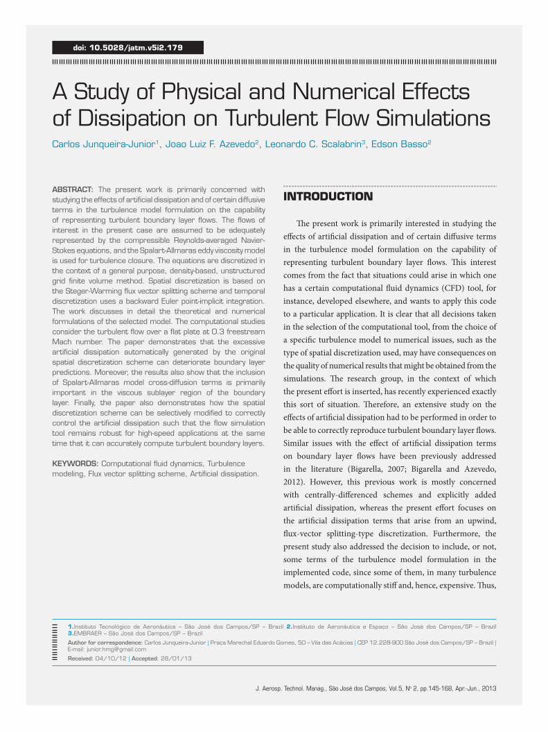
In order to avoid sudden sign transitions, as illustrated in Fig. 1, the split eigenvalues receive a small number, ϵ, turning Eq. (20) into

λ± = 12

λ ± λ 2 + ϵ 2 .( )√ (21)

Numerical studies performed in the present paper indicated that this flux vector splitting is too dissipative and it can deteriorate the boundary layer profiles (MacCormack and Candler, 1989; Junqueira-Junior et al., 2011). To avoid such

issue a pressure switch is implemented to smoothly shift the Steger-Warming scheme into a centered one. Then, the artificial dissipation is controlled and the numerical stability is maintained as presented in

→ →F ek· nk = F +k + F−k = A+

k+ Qk+ + A−

k−Q

k−,( ) (22)

in which

Qk+= (1−w)Qcl +wQcr and Qk−= (1−w)Qcr+wQcl . (23)

The switch, w, is given by

w = 12

1(α∇p)2 + 1 and ∇p = |pcl − pcr |

min (pcl , pcr). (24)

Therefore, for small ∇p, w = (1–w) = 0.5, the code runs with a centered scheme, and for larger values of ∇p, w = 0 and (1–w) = 1, the code runs with the Steger-Warming scheme. For Eq. (24), it is suggested α = 6, but some problems may require larger values (Scalabrin, 2007).

The applied formulation was originally created with interest on studying flows over reentry capsules. For this particular case, with very strong shock waves, it is very common to find solutions with nonphysical numerical structures such as carbuncles (Ramalho et al., 2011). To prevent such numerical problems, artificial dissipation has necessarily to be added to the method. The dissipation was included into the split eigenvalues, Eq. (21), using the ϵ factor, which is given by:

λ

λ+

Change of SignEigenvalues

SuddenSmooth

0.100.090.080.070.060.050.040.030.020.01

-0.05 0.05-0.04 0.04-0.03 0.03-0.02 0.02-0.01 0.010.00

Figure 1. Sudden (Eq. 20) and smooth (Eq. 21) sign transition of a given Eigenvalue.



k = 0.3(ak + |→uk |) dk > d00.3(1 − |→nk · →mk |)(ak + |→uk |) dk < d0

,ϵ ⎨⎧

⎩ (25)

where dk is the distance of the k-th face to the the nearest wall boundary, d0 is set by the user and must be smaller than the boundary layer thickness and larger than the shock stand-off distance, mk

→ is the normal vector of

the nearest wall, and nk→

is the normal vector to the k-th face. Equation (25) applies the term (1 - |nk

→ ·mk

→|) to decrease the

ϵ value at the faces parallel to the wall inside the boundary layer (Scalabrin, 2007). This artificial dissipation model has shown an important role in the prediction of boundary layer profiles, and several tests were performed in the present work with the aim of understanding its behavior (Junqueira-Junior et al., 2011).

Viscous flux calculation The viscous terms are based on derivative of properties

on the faces. To build the derivative terms, two volumes are created over the face where the derivative is being calculated. At the center of each new volume, the derivative is calculated using the Green-Gauss theorem. This computation is used to find the derivative at the desired face.

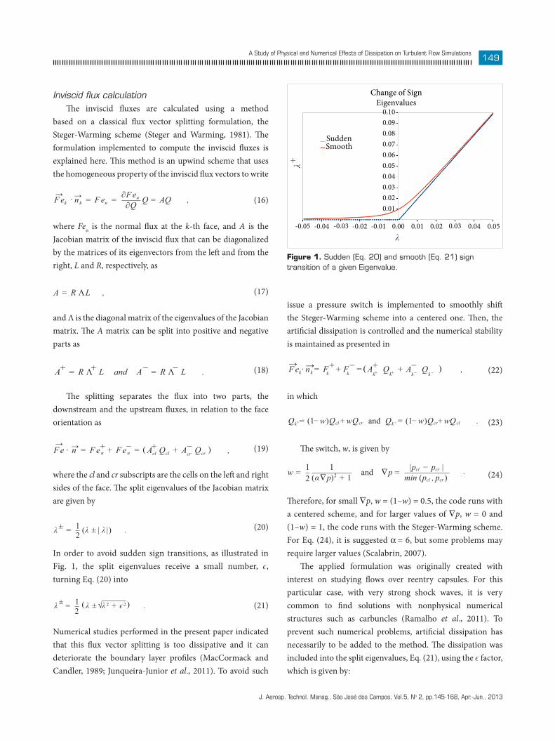
A two-dimensional (2-D) example is used in this section to better explain the derivative calculation. Considering the two cells, S1 and S2, in Fig. 2, two new cells, S3 and S4,

are created using node points, P1 and P3, and cell centered points, P2 and P4, to calculate the derivative on the face 1-3.

The properties at the faces are calculated using simple averages. For the example in Fig. 2, they are given by

Q12 = 12

(Q1 + Q2 ) ,

Q23 = 12

(Q2 + Q3 ) ,

Q13 = Q31 = 12

(Q1 + Q3 ) ,

Q34 = 12

(Q3 + Q4 ) ,

Q41 = 12

(Q4 + Q1 ) .

(26)

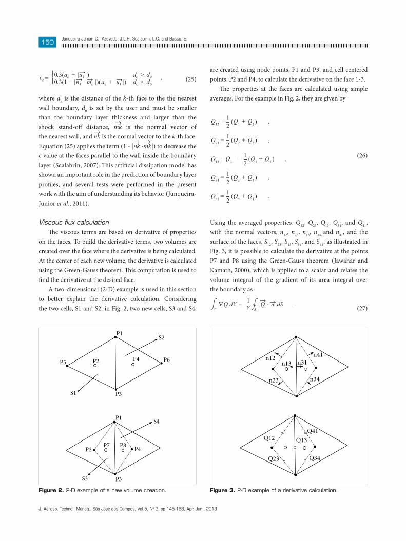
Using the averaged properties, Q12, Q23, Q13, Q34, and Q41, with the normal vectors, n12, n23, n13, n34, and n41, and the surface of the faces, S12, S23, S13, S34, and S41, as illustrated in Fig. 3, it is possible to calculate the derivative at the points P7 and P8 using the Green-Gauss theorem (Jawahar and Kamath, 2000), which is applied to a scalar and relates the volume integral of the gradient of its area integral over the boundary as

V∇Q dV = 1

V S

→Q · →n dS .⌠⌡

⌠⌡ (27)

P1

P2

P3

P3

P1

P4 P6

S2

P5

S1

P7 P8P2 P4

S3

S4

Figure 2. 2-D example of a new volume creation.

n12n13

Q12

Q23

Q13Q41

Q34

n31n41

n34n23

Figure 3. 2-D example of a derivative calculation.



Considering ∇Q as a constant over the cell, Eq. 27 yields

∇Q = 1V

→Q · →n dS ,S

⌠⌡ (28)

in which ∇Q is the constant cell-centered gradient. Using the derivatives in the cells S3 and S4, the derivative at face 1-3 is computed using

∇ ∇ ∇Q13 = V3 Q3 + V4 Q4

V3 + V4

. (29)

The derivative computation for other types of element, 2D or 3D, is straightforward.

time integrAtion Simulations of turbulent flows can become very stiff. Such

stiffness substantially limits the use of large time steps. One classical solution is the use of implicit time integration. This work applies an implicit integration based on the backward Euler method, which is given by

∆Qncl

∆ t Vcl = −nf

k =1

→F ek −→F vk · →nk Sk

n +1

= Rn +1

cl .⎡⎣

⎤⎦∑ ( ) (30)

One can linearize the residue at time n+1 as a function of properties at time n.

∆Qncl

∆ t Vcl = R ncl −

nf

k =1

∂ →F e · →n∂Q

n

k∆Q n

cl−

∂ →F v · →n∂Q

n

k∆Q

n

cl · Sk .

∑⎧⎨⎩

⎫⎬⎭

⎡⎜⎣

⎜⎤

⎦

⎡⎜⎣

⎜⎤

⎦

( )

( ) (31)

From the spatial discretization, the inviscid terms can be written as

∂ →F e · →n∂Q

k

∆Qcl=∂ F e+ · →→ n

∂Qk

∆Qcl +

∂ →F e− · →n∂Q

k

∆Qcl ,

⎡⎜⎣

⎜⎤

⎦

⎡⎜⎣

⎜⎤

⎦

⎡⎜⎣

⎜⎤

⎦

( )

( )

( ) (32)

with

∂ F e+ · →→ n∂Q k

∆Qcl = A+k + ∆Qcl

⎡⎜⎣

⎜⎤

⎦

( ) (33)

and

→∂ F e− · →n∂Q

k

∆Qcl = A−k− ∆Qcr .⎡⎜⎣

⎜⎤

⎦( )

(34)

The formulation described assumes

→∂ F e± · →n∂Q = A± ,

⎡⎜⎣

⎜⎤

⎦( ) (35)

which is not true and can decrease the numerical stability of the method. Then, the true Jacobian matrices of the split fluxes were implemented in place of A± to calculate the implicit operator. Issues involving the true Jacobians matrices have a great importance in the context of numerical stability for computational methods. The reader with interest in this subject must look further in references Anderson et al. (1986) and Steger and Warming (1981), and in chapter 20 from Hirsch (1990).

The viscous terms can be written in the same form as

∂ →F v · →n∂Q k

∆Qcl =∂ →F v− ·

→n∂Q k

∆Qcl −

∂ →F v+ · →n∂Q k

∆Qcl .

⎡⎜⎣

⎜⎤

⎦

⎡⎜⎣

⎜⎤

⎦⎡⎜⎣

⎜⎤

⎦

( ) ( )

( )

(36)

The viscous Jacobian matrices are represented by B. The splitting of these matrices is written as

∂ F v · →→ n∂Q

k

∆Qcl =B−k− ∆Qcr,k −B+k+ ∆Qcl .

⎡⎜⎣

⎜⎤

⎦( ) (37)

The true Jacobian matrices, for A± and B±, can be found in the work of Scalabrin (2007). One can write the system as

Vcl∆ t +

nf

k =1A+

k+ + B+k+ Sk ∆Q +

nf

k =1

A−k− − B−k− Sk ∆Qn

cr,k = R n

cl

n

cl

.

∑

∑

⎡⎜⎣

⎜⎤

⎦⎡⎜⎣

⎜⎤

⎦

( ) (38)

It is, then, possible to write

Mcl ∆ Qncl +

nf

k =1N−

k ∆ Qncr,k =R n

cl ,∑ (39)

with

Mcl =Vcl

∆ t

nf

k =1N +

k ,∑ (40)



N +k = A+

k+ + B+k+ S k ,( ) (41)

and N−

k = A−k− −B−k− S k .( ) (42)

As the code is an unstructured solver, this system of equations results in a sparse block matrix, where each block is a square matrix of size equal to the number of equations to be solved in each control volume. The solution of such system is typically very expensive and, depending on the size of the mesh, it is not even practical. A less expensive implicit method is applied in the present paper, the point implicit integration (Gnoffo, 2003; Venkatakrishnan, 1995; Wright, 1997).

The main idea of the point implicit integration is to move all the off-diagonal terms to the right hand side and solve the resulting system iteratively, i.e.,

Mcl ∆ Qn +1,pcl = R n

cl −nf

k =1N −

k ∆ Qn +1,p −1cr,k .∑ (43)

It is assumed that ∆Qn+1,0 = 0 and four iterations are taken in the process as suggested in the literature (Wright, 1997). The sparse linear system illustrates the point implicit method:

∆ Q ( n +1) = Rn ,

∆ Q ( n +1) ,p = R n −

∆Q ( n +1) ,p −1 .

⎡⎜⎜⎜⎜⎣

⎜⎜⎜⎜

⎤

⎦

⎡⎜⎜⎜⎜⎣

⎜⎜⎜⎜

⎤

⎦

⎡⎜⎜⎜⎜⎣

⎡⎜⎜⎜⎜⎣

⎜⎜⎜⎜

⎤

⎦

⎡⎜⎜⎜⎜⎣

⎡⎜⎜⎜⎜⎣

⎡⎜⎜⎜⎜⎣

⎡⎜⎜⎜⎜⎣

⎜⎜⎜⎜

⎤

⎦

⎜⎜⎜⎜

⎤

⎦

⎜⎜⎜⎜

⎤

⎦

⎜⎜⎜⎜

⎤

⎦

⎜⎜⎜⎜

⎤

⎦

Each , in the sparse matrix, is a block matrix.The time step is computed by

∆ t = CF L

||→v || + a, (44)

in which CFL (Azevedo, 1988) is a parameter set to ensure stability of the time integration method, l is the size of the cell and || -v || + a is the largest wave speed in the cell (Scalabrin, 2007).

second-order extension of inviscid fluxes The monotone upstream-centered scheme for conservation

laws, known as MUSCL approach (van Leer, 1979), is used

in order to obtain second-order extension for the inviscid fluxes calculation. This section presents the classical formulation of the MUSCL approach and an extension for unstructured grids.

MUSCL approach A first-order spatial discretization is equivalent to represent

the numerical approximation of the solution as a piecewise constant. The MUSCL idea is to use a linear approximation to achieve a second-order space discretization. A linear solution is exactly resolved, which generates a truncation error of the order ∆x2. In order to represent the conservation laws, the discrete state variables express the average state within the cells. Then, the linear approximation has to average out these values (Hirsch, 1990).

One can consider the Taylor linearization as a one-dimensional (1-D) local representation, Fig. 4, valid in a given cell “i”, at a determined instant

Q(x ) = Qi+1∆ x

(x−x i ) δi Q+O ∆ x 2 xi −1/2<x<xi +1/2 .( ) ( ) (45)

setting x = xi ± ∆x/2, it is possible to write

QLi +1/2 = Qi+ 1

∆ x xi + ∆ x2 −xi δi Q =Qi + 1

2δi Q ,( ) (46)

QRi−1/2 = Qi+ 1

∆ x xi−∆ x2 −xi δi Q =Qi−

12δi Q .( ) (47)

The use of backward and forward derivatives provides

QLi + 1/2 = Qi + 1

2Qi−Qi− 1 ,( ) (48)

QRi−1/2 = Qi−

12

Qi +1−Qi .( ) (49)

One can rewrite these terms at the same faces as

QLi + 1/2 (x) = Qi + 1

2Qi −Qi− 1 ,( ) (50)

QRi + 1/2 (x ) = Qi +1−

12

Qi +2−Qi +1 .( ) (51)

Using limiters to treat correctly the discontinuities, the MUSCL scheme can be written as

QLi + 1/2 (x ) = Qi + 1

2ψ rL Qi−Qi− 1 ,( )( ) (52)

QRi + 1/2 (x ) = Qi +1−

12ψ rL Qi +2−Qi +1 ,( ) ( ) (53)



where r is the ratio of consecutive variations, given by rL=

Qi +1 − Qi

Qi − Qi− 1

, rR=Qi +1 − Qi

Qi +2 − Qi +1, (54)

and ψ(r) is a limiter function. Th ese functions are extremely important in the context of high-order methods. However, this discussion is not in the scope of the present work. One can fi nd further information about limiter functions in chapter 21 from Hirsch (1990).

Th ere are several limiter functions available for high-order methods of CFD applications. Two of these functions are implemented herein, the van Albada limiter (van Albada et al., 1982), given by

ψ (r ) = r 2 + r1 + r 2 , (55)

and the minmod limiter (Hirsch, 1990), written as

ψ (r ) = min [r , 1] , r> 00 , r ≤ 0 .⎧⎨⎩

(56)

Th e simulations performed in the present work used mainly the van Albada limiter function (Hirsch, 1990).

Second-order extension for unstructured grids Th e MUSCL variable extrapolation for 2-D or 3-D is

straightforward for structured meshes. However, it is not very simple for unstructured solvers. Th e approach applied here is based on the work of Batina (1990) and Bibb et al. (1997). Here, the stencils are created using only cell-centered values. Th e points “i” and “i+1” are, respectively, the center of the cell at the left and right of the face. Th e other two points, “i-1” and “i+2”, are defi ned by a stencil search.

Th e search for cells “i+2” and “i-1” is limited to the ones that share at least one node with the volumes “i+1” and “i”, respectively. Th e selected “i+2” point is the one that has the maximum positive value of the dot product between the face normal and the normalized vector joining the face centroid

to cell centroid. Using the same principle, the chosen “i-1” point is the one with the maximum negative value of the dot product. Figure 5 is extracted from Scalabrin (2007), and illustrates the search for the “i+2” point in a given mesh.

It is possible to observe that, when the stencil search is applied to unstructured grids, the distance between the “i+1” and “i+2” points can be diff erent from the distance between the “i” and “i+1” points. Th erefore, a correction is applied on the limiter, as given by

rL=Qi +1 − Qi

Qi − Qi− 1

ba

, rR=Qi +1 − Qi

Qi +2 − Qi +1

ca

, (57)

where “a” is the distance between the “i+1” and “i” points, “b” is the distance between the “i+2” and “i+1”points, and “c” is the distance between the “i” and “i-1” points.

TURBULENCE MODELING

the spAlArt-AllmArAs turbulence model Th e Spalart-Allmaras (SA) closure (Spalart and Allmaras,

1992 and 1994) is a one-equation, linear eddy-viscosity turbulence model. It solves one transport equation for the modifi ed eddy viscosity coeffi cient, ~ν . Th e model uses eight closure coeffi cients and three closure functions derived along intuitive and empirical lines, relying heavily on calibration by reference to a wide range of experimental data (Spalart

Figure 5. Search for the “i + 2” point inside an unstructured grid. (Scalabrin, 2007).

Not selectedSelected

i+1

i

i+2i-1 i

i+1/2

i+1

i-1/2

Figure 4. 1-D local representation of a fi nite volume grid.



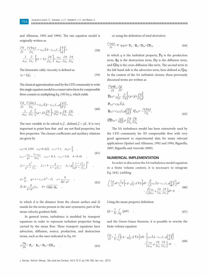
and Allmaras, 1992 and 1994). The one equation model is originally written as

∂ ν∂t

+ ∂ (νuj )∂xj

= cb1 S ν−cw1 f wνd

2+

1σSA

∂∂xj

(ν + ν ) ∂ ν∂xj

+ cb2

σSA

∂ ν∂xk

∂ ν∂xk

.

⎛⎝

⎞⎠

⎡⎣

⎤⎦

(58)

The kinematic eddy viscosity is defined as νt = νfv1 . (59)

The classical approximation used by the CFD community to write this single equation model in a conservative form for compressible flows consists in multiplying Eq. (59) by ρ, which yields

∂ µ∂t

+∂ (µuj )∂xj

=cb1 S µ−cw1 f w ρ νd

2+

1σSA

∂∂x j

(µ+µ) ∂ ν∂xj+ cb2σSA

ρ ∂ ν∂xk

∂ ν∂xk

.

⎛⎝⎞⎠

⎡⎣

⎤⎦

(60)

The new variable to be solved is μ , defined μ = ρν . It is very important to point here that and are not fluid properties, but flow properties. The closure coefficients and auxiliary relations are given by

cb1=0 .1355, cb2=0 .622, cv 1=7.1, σSA= 23

,

cw1 = cb1

k 2 + 1+cb2σSA

, cw2= 0.3, cw 3 =2.0, k =0 .41 ,

fv1=χ3

χ3 + c3v 1

, f v2 =1− χ1 + χ f v 1

, f w=g 1 + c6w 3

g6 + c6w 3

16

,⎡⎣

⎤⎦

(61)

( )χ= νν , g= r + cw 2 r 6− r , r= ν

Sk 2 d 2,

S=S+ νk 2 d 2

fv2 , S= ,2Ωij Ωij√¯¯¯ ¯ ¬ (62)

in which d is the distance from the closest surface and Ω stands for the terms present in the anti-symmetric part of the mean velocity gradient field.

In general terms, turbulence is modeled by transport equations in order to represent turbulent properties being carried by the mean flow. These transport equations have advection, diffusion, source, production, and destruction terms, such as the ones indicated in Eq. 63:

ρDqDt

= ρq− ρq+ ρq+ ρq , (63)

or using the definition of total derivative:

∂ (ρq)∂t

+∇ ∙ ρqv =Pρq −Sρq+Dρq+CDρq .( ) (64)

in which q is the turbulent property, Pq is the production term, Sq is the destruction term, Dq is the diffusion term, and CDq is the cross-diffusion-like term. The second term in the left-hand side is the advection term, here defined as Cpq. In the context of the SA turbulent closure, these previously discussed terms are written as

∂ (ρq)∂t

=∂µ∂t ,

DSA= 1σSA

∂∂xj

(µ+µ) ∂ ν∂xj,

PSA=cb1 S µ

SSA=cw1 fwρ νd

2, CSA= ∂(µuj)

∂xj,

CDSA= cb2σSA ρ

∂ ν∂xk

∂ν∂xk

.

⎡⎣

⎤⎦

⎛⎝⎞⎠

,

(65)

The SA turbulence model has been extensively used by the CFD community for 3D compressible flow with very good agreement to experimental data for many relevant applications (Spalart and Allmaras, 1992 and 1994; Bigarella, 2007; Bigarella and Azevedo 2009).

numericAl implementAtion In order to discretize the SA turbulence model equation

in a finite volume context, it is necessary to integrate Eq. (64), yielding

Vi

∂ µ∂t

dV+Vi

∇· v µ− 1σSA

µ ∇µ dV−Vi

cb1 S µ−cw 1 f w ρ νd

2dV

−Vi

cb2

σSAρ ∂ ν∂xk

∂ ν∂xk

dV=0 .

⎡⎣

⎤⎦

⎡⎣

⎤⎦

⎡⎣

⎤⎦

⎛⎝⎞⎠

⌠⌡

⌠⌡

⌠⌡

⌠⌡^

(66)

Using the mean property definition

Qi = 1Vi Vi

QdVi ,⌠⌡ (67)

and the Green-Gauss theorem, it is possible to rewrite the finite volume equation

∂ µi

∂t+ 1

Vi Si

v µ − 1σSA

µ µ ·dS − cb1 S µ−cw 1 f w ρ νd

2

+ cb2

σSAρ ∂ ν∂xk

∂ ν∂xk

=0 .

⎡⎣

⎤⎦

⎡⎣

⎤⎦

⎛⎝

⎞⎠

⎛⎝

⎞⎠

⌠⌡ ∇^

(68)



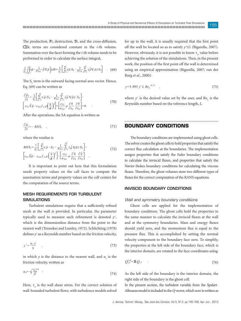
The production, Pi, destruction, Si, and the cross-diffusion, CDi, terms are considered constant in the i-th volume. Summation over the faces forming the i-th volume needs to be performed in order to calculate the surface integral,

1Vi Si

vµ− 1σSA

µ µ ·dS≡ 1Vi

nf

k=1vµ·Sk− 1

σSA

nf

k=1(µ µ)·S k .⎡

⎣⎤⎦

⎛⎝

⎞⎠

⌠⌡ ∇^ ∇^∑ ∑ (69)

The Sk term is the outward facing normal area vector. Hence, Eq. (69) can be written as

∂ µi

∂t+ 1

Vi

nf

k =1v µ·S k − 1

σSA

nf

k =1(µ µ)· S k −

cb1 S µ−cw1 f w ρ νd

2+ cb2

σSAρ ∂ ν∂xk

∂ ν∂xk

=0 .⎡⎣

⎡⎣

⎤⎦

⎤⎦

⎡⎣

⎤⎦

⎛⎝

⎞⎠

∇^∑ ∑

(70)

After the operations, the SA equation is written as

∂ µi

∂t=−RHSt , (71)

where the residue is

RHSt =1Vi

nf

k =1v µ · S k− 1

σSA

nf

k =1(µ µ)·S k −

cb1 Sµ− cw1 f w ρνd

2− cb2

σSAρ ∂ ν∂xk

∂ ν∂xk

.

⎡⎣

⎡⎣

⎡⎣

⎤⎦

⎤⎦

⎤⎦

⎛⎝

⎞⎠

∇^∑ ∑ (72)

It is important to point out here that this formulation needs property values on the cell faces to compute the summation terms and property values on the cell centers for the computation of the source terms.

mesh requirements for turbulent simulAtions

Turbulent simulations require that a sufficiently refined mesh at the wall is provided. In particular, the parameter typically used to measure such refinement is denoted y+, which is the dimensionless distance from the point to the nearest wall (Tennekes and Lumley, 1972). Schlichting (1978) defines y+ as a Reynolds number based on the friction velocity,

y+= u τ yν

, (73)

in which y is the distance to the nearest wall, and uτ is the friction velocity, written as

u τ= τwρ.√ ¬¯ (74)

Here, τw is the wall shear stress. For the correct solution of wall-bounded turbulent flows, with turbulence models solved

for up to the wall, it is usually required that the first point off the wall be located so as to satisfy y+≤1 (Bigarella, 2007). However, obviously, it is not possible to know τw value before achieving the solution of the simulations. Then, in the present work, the position of the first point off the wall is determined using an empirical approximation (Bigarella, 2007; van der Burg et al., 2000):

y=5 .893 y+L Re −0 . 9L , (75)

where y+ is the desired value set by the user, and ReL is the Reynolds number based on the reference length, L.

BOUNDARY CONDITIONS

The boundary conditions are implemented using ghost cells. The solver creates the ghost cells to hold properties that satisfy the correct flux calculation at the boundaries. The implementation assigns properties that satisfy the Euler boundary conditions to calculate the inviscid fluxes, and properties that satisfy the Navier-Stokes boundary conditions for calculating the viscous fluxes. Therefore, the ghost volumes store two different types of fluxes for the correct computation of the RANS equations.

inviscid boundAry conditions

Wall and symmetry boundary conditions Ghost cells are applied for the implementation of

boundary conditions. The ghost cells hold the properties in the same manner to calculate the inviscid fluxes at the wall and at the symmetry boundaries. Mass and energy fluxes should yield zero, and the momentum flux is equal to the pressure flux. This is accomplished by setting the normal velocity component to the boundary face zero. To simplify, the properties at the left side of the boundary face, which is the interior domain, are rotated to the face coordinates using

Qrotcl =RQcl . (76)

As the left side of the boundary is the interior domain, the right side of the boundary is the ghost cell. In the present section, the turbulent variable from the Spalart-Allmaras model is included in the Q vector, which now is written as



Q = [ ρ ρu ρv ρw e µ ] T . (77)

In Eq. (76), is the rotation matrix given by,

R=

1 0 0 0 0 00 n x n y n z 0 00 t x t y t z 0 00 rx ry rz 0 00 0 0 0 1 00 0 0 0 0 1

⎡⎜⎜⎜⎜⎜⎣ ⎡

⎜⎜⎜⎜⎜⎣

, (78)

and the n→, t→, r→ vectors define the face-based reference frame. The properties at the ghost cells are set to

ρcr=ρcl ,

ρcr urotcr,n =−ρcl urot

cl,n ,

ρcr urotcr, t =ρcl urot

cl,t ,

ρcr urotcr,r =ρcl urot

cl,r ,

ei cr= ei cl ,

µcr= µcl .

(79)

One can write in the matrix form as

Qrotcr =W Q ,rot

cl (80)

in which W is the inviscid wall matrix given by

W=

1 0 0 0 0 00 −1 0 0 0 00 0 1 0 0 00 0 0 1 0 00 0 0 0 1 00 0 0 0 0 1

⎡⎜⎜⎜⎜⎜⎣ ⎡

⎜⎜⎜⎜⎜⎣

.

(81)

Therefore, the boundary condition can be written as

Qcr=R− 1WRQcl , (82)

in which the R-1 matrix is given by

−1=

1 0 0 0 0 00 n x t x rx 0 00 n y t y ry 0 00 n z t z rz 0 00 0 0 0 1 00 0 0 0 0 1

.

⎡⎜⎜⎜⎜⎜⎣ ⎡

⎜⎜⎜⎜⎜⎣

(83)

It returns the properties to the Cartesian coordinate frame.

Nonreflecting farfield boundary condition The concept of Riemann invariants (Long et al., 1991;

Bigarella, 2007) is implemented to achieve a nonreflecting farfield boundary condition at subsonic speeds. These

invariants are derived from the characteristic relations for the Euler equations. The formulation at the boundary is given by Ri −= Ri −∞ = vn∞ − 2

γ − 1 a∞ ,

Ri +=Ri +int =vnint + 2

γ − 1 aint , (84)

in which vn is the normal velocity component given by vn= v→· n→. The subscripts ∞ and int represent the property at the freestream and in the interior domain, respectively. The normal velocity component and the speed of the sound at the boundary face can be written as

vnf = Ri+int + Ri −∞

2 ,

af = γ − 14 Ri +

int+ Ri −∞ ,

(85)

in which the f subscript represents the property at the farfield computational surface.

It is possible to write the velocity for a subsonic exit, 0 < vn int / aint < 1, using the tangential velocity components of the interior and the definition of normal velocity.

uf=uint+ (vnf−vn int )· nx ,vf =vint+ (vnf−vn int )· ny ,wf=wint+ (vnf−vn int )· nz .

(86)

The other properties are given by

ρf =ργint a2

fγpint

1γ−1

pf =ρf a2

fγ

ef = pf

(γ−1)+ 1

2ρf u2

f + v2f + w2

f

µf =µint

⎛⎝

⎞⎠

( )

,

,

,

.

(87)

For a subsonic entrance boundary, -1 < vn int / aint < 0, one should extrapolate the freestream properties as

uf =u∞+(vnf +vn∞)· nx ,vf =v∞+(vnf +vn∞)· ny ,wf =w∞+(vnf +vn∞)· nz ,

(88)

ρf = ργ∞ a2f

γp ∞

1γ − 1

pf =ρf a2

f

γ

ef =

=

pf

( γ−1)+1

2ρf u2

f +v2f +w2

f

µf µ∞

⎛⎝

⎞⎠

( )

,

,

,

.

(89)



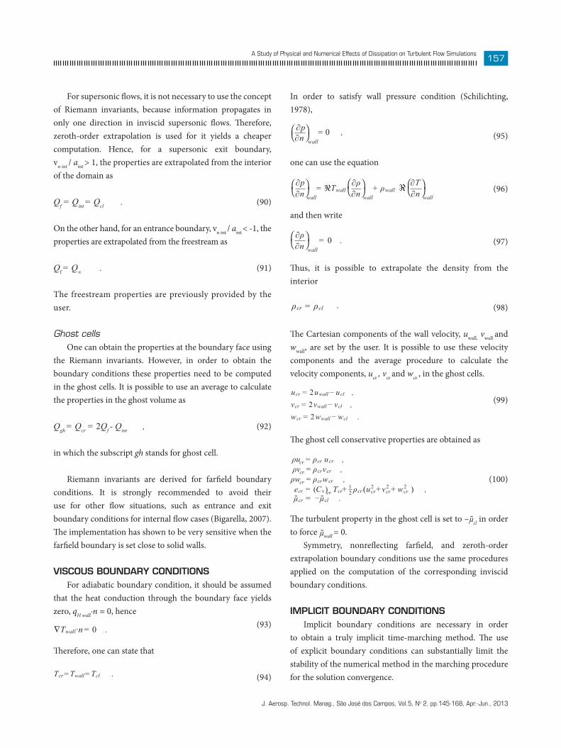
For supersonic fl ows, it is not necessary to use the concept of Riemann invariants, because information propagates in only one direction in inviscid supersonic fl ows. Th erefore, zeroth-order extrapolation is used for it yields a cheaper computation. Hence, for a supersonic exit boundary, vn int / aint > 1, the properties are extrapolated from the interior of the domain as

Qf = Qint = Qcl . (90)

On the other hand, for an entrance boundary, vn int / aint < -1, the properties are extrapolated from the freestream as

Qf = Q∞ . (91)

The freestream properties are previously provided by the user.

Ghost cells One can obtain the properties at the boundary face using

the Riemann invariants. However, in order to obtain the boundary conditions these properties need to be computed in the ghost cells. It is possible to use an average to calculate the properties in the ghost volume as

Qgh = Qcr = 2Qf - Qint , (92)

in which the subscript gh stands for ghost cell.

Riemann invariants are derived for farfi eld boundary conditions. It is strongly recommended to avoid their use for other fl ow situations, such as entrance and exit boundary conditions for internal fl ow cases (Bigarella, 2007). Th e implementation has shown to be very sensitive when the farfi eld boundary is set close to solid walls.

viscous boundAry conditions For adiabatic boundary condition, it should be assumed

that the heat conduction through the boundary face yields zero, qH wall·n = 0, hence

∇Twall·n = 0 . (93)

Th erefore, one can state that

Tcr =Twall=Tcl . (94)

In order to satisfy wall pressure condition (Schilichting, 1978),

∂p∂n wall

,0=⎛⎝

⎞⎠ (95)

one can use the equation

∂p∂n wall

= Twall∂ρ∂n wall

+ ρwall∂T∂n wall

⎛⎝

⎞⎠

⎛⎝

⎞⎠

⎛⎝

⎞⎠T (96)

and then write

∂ρ∂n wall

. 0=⎛⎝

⎞⎠ (97)

Th us, it is possible to extrapolate the density from the interior

ρcr = ρcl . (98)

Th e Cartesian components of the wall velocity, uwall, vwall and wwall, are set by the user. It is possible to use these velocity components and the average procedure to calculate the velocity components, ucr , vcr and wcr , in the ghost cells.

ucr = 2uwall−ucl ,vcr = 2vwall−vcl ,wcr = 2wwall−wcl .

(99)

Th e ghost cell conservative properties are obtained as

ρucr = ρcr u cr ,ρvcr = ρcrvcr ,ρwcr = ρcrwcr ,ecr = (Cv)cr Tcr+ 1

2 ρcr u2cr+v2

cr+w2cr ,

µcr = −µcl .( )

(100)

Th e turbulent property in the ghost cell is set to –µcl in order to force µwall = 0.

Symmetry, nonrefl ecting farfi eld, and zeroth-order extrapolation boundary conditions use the same procedures applied on the computation of the corresponding inviscid boundary conditions.

implicit boundAry conditions Implicit boundary conditions are necessary in order

to obtain a truly implicit time-marching method. Th e use of explicit boundary conditions can substantially limit the stability of the numerical method in the marching procedure for the solution convergence.



bAsic implicit formulAtion A simplified form of the implicit equation, Eq. (38), is

written in this section in order to detail the implementation of implicit boundary conditions for flux vector splitting schemes:

Vcl

∆ t+ A+

k+ + B +k+ Sk ∆Qcl +

A−k− −B−

k− Sk ∆Qcr,k=R ncl .

( )

( )

⎡⎣

⎤⎦

]]

(101)

In such equation, the repeated k index in the second term in left hand side of the equation indicates summation over all the k faces of the control volume. Equation (101) is written only to present the relation between an internal cell, cl, and a boundary cell, cr, k. In the original formulation, Eq. (38), the cl-th cell has contributions from other faces, which may or may not be boundaries.

As presented in the beginning of this section, the ghost cells hold different values for inviscid and viscous calculations. Hence, using the splitting definition, presented in section numerical formulation, Eq. (101) can be written as

Vcl

∆ t+ A+

k+ +B +k+ Sk ∆Qcl +A−

k− Sk ∆ Qcr,k,inv

−B−k− Sk ∆ Qcr,k,visc =R n

cl .

⎡⎣

⎤⎦( )

(102)

The contributions of the boundary face can be expressed in terms of the internal cell corrections as

∆ Qcr,k,inv= k,inv∆ Qcl ,F (103)

∆ Qcr,k,visc= k,visc∆Qcl .F (104)

Hence, Eq. (102), can be rewritten as

Vcl

∆ t+ A+

k++ A−k− k,inv−B−

k− k,visc+ B +k+ Sk ∆Qcl =R n

cl .( ) ⎤⎦F F⎡

⎣ (105)

The viscous Jacobians are calculated using primitive variables, and the corrections are set for the primitive variables and applied directly at the calculation of the viscous Jacobians. The matrix B+

k+

already includes the contribution from the boundary. The A+k+ ,

A–k– , B+

k+ and B–k– are presented in the work of Scalabrin (2007).

Inviscid boundary conditions The matrix for an inviscid wall or for a symmetry

boundary is the same presented in Eq. (82),

k, inv, wall = −1 W ,k, inv, sym= −1 W .

FF (106)

The matrices are applied to ∆Q for the implicit boundary condition according to Eq. (104).

It is possible to use the identity matrix to represent the zeroth-order extrapolation as given by

k,inv= [ I ] .F (107)

For the purpose of developing the implicit boundary condition, the farfield variables are considered constant. Hence, ∆Q at a farfield boundary is given by

∆ Qcr,k = 0 , (108)

which implies in

k,inv = 0 ,F (109)

where 0 stands for the zero matrix.

Viscous boundary conditions The viscous Jacobians are created using primitive

variables. Therefore, the implementation of implicit viscous matrices is performed using primitive variables. They are applied directly at the calculation of the Jacobians matrices as

V= ρ u v w T νT .[ ] (110)

The adiabatic wall implicit boundary condition is calculated using

F k,visc =

0 0 0 0 0 00 −1 0 0 0 00 0 −1 0 0 00 0 0 −1 0 00 0 0 0 1 00 0 0 0 0 −1

⎡⎜⎜⎜⎜⎜⎣

⎡⎜⎜⎜⎜⎜⎣

(111)

The same procedure used for the inviscid zeroth-order extrapolation is used here, hence

Fk,visc = [ I ] . (112)



Th e viscous farfi eld matrix is the same one used for the inviscid farfi eld boundary condition, which is given by

F Fk,visc = k,inv =0 , (113)

in which 0 stands for the zero matrix.

FLOW SIMULATION RESULTS AND DISCUSSION

Th e test case used in this work is the simulation of turbulent subsonic fl ow over a fl at plate geometry in absence of streamwise pressure gradients. Th e work studies the addition of diff erent levels of artifi cial dissipation, at diff erent distances of the wall, in an attempt to fully understand the eff ects of the high dissipative upwind spatial discretization over turbulent dimensionless boundary layer profi les and over the friction coeffi cient. All results are compared to analytical and experimental data. Th e Mach number at the freestream condition is set to M∞ = 0.3, and the Reynolds number based on 1 m long fl at plate is 7.2 million. Th erefore, the fl ow can be considered as a turbulent compressible fl ow. Th e computational domain covers a 3 m high and 7 m long region. Th e wall fl at plate is located between 3< x <4. As illustrated in Fig. 6, the applied boundary conditions are as follows: in the lower portion of the computational domain, symmetry is used between the entry and the fl at plate, and between the trailing edge and the outlet; an adiabatic wall is assumed over the fl at plate surface; and farfi eld Riemann-type boundary conditions are used for all the other boundaries. Th e simulations are performed using two grids, one with 60,000 cells and another with 210,000 cells, as illustrated in Fig. 7. Both meshes have y+ = 0.5 at the fi rst grid point off the wall, but the mesh with 210,000 cells has more points near to the wall.

Th e dimensionless boundary layer profi les obtained by the simulations are compared to the analytical formulation given by the law of wall (Schilichting, 1978), which is written by

y+< viscous sublayer u+= y+

30

5

< y+<300 log-law region u+= 10.41

ln (y+)+5.5 .

⎧⎨⎩ (114)

Th e distribution of the local skin friction coeffi cient, cf , which is written as

cf = τw12 ρ∞ u2

∞, (115)

is compared to experimental data (Coles and Hirst, 1969), and to the analytical formulation (von Karman, 1934) given by

cfvon Karman (Rex ) = 0 .025 Re − 17x , (116)

3

2

1

0

3

2

1

0

0 1 2 3 4 5 6 7

0 1 2 3 4 5 6 7

YY

X

X

(a)

(b)

Figure 7. Visualization of the meshes used in the zero-pressure-gradient fl ow over a fl at plate. (a) Mesh with 60,000 volumes; (b) Mesh with 210,000 volumes.

3

2

1

0 1

Symmetry Symmetry

Fareld

Fareld

Fareld

Wall

2 3 4 5 6 7

Y

X

Figure 6. Domain used for the zero-pressure-gradient fl ow over a fl at plate.



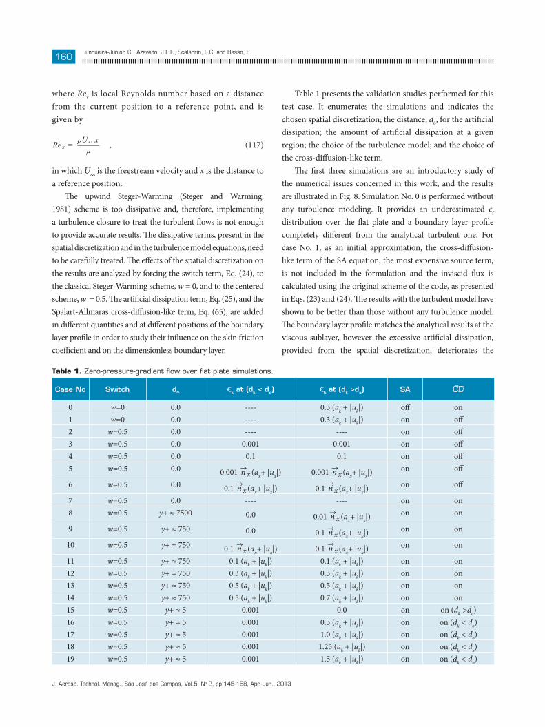
where Rex is local Reynolds number based on a distance from the current position to a reference point, and is given by

Rex = ρU∞ xµ

, (117)

in which U∞ is the freestream velocity and x is the distance to a reference position.

The upwind Steger-Warming (Steger and Warming, 1981) scheme is too dissipative and, therefore, implementing a turbulence closure to treat the turbulent flows is not enough to provide accurate results. The dissipative terms, present in the spatial discretization and in the turbulence model equations, need to be carefully treated. The effects of the spatial discretization on the results are analyzed by forcing the switch term, Eq. (24), to the classical Steger-Warming scheme, w = 0, and to the centered scheme, w = 0.5. The artificial dissipation term, Eq. (25), and the Spalart-Allmaras cross-diffusion-like term, Eq. (65), are added in different quantities and at different positions of the boundary layer profile in order to study their influence on the skin friction coefficient and on the dimensionless boundary layer.

Table 1 presents the validation studies performed for this test case. It enumerates the simulations and indicates the chosen spatial discretization; the distance, d0, for the artificial dissipation; the amount of artificial dissipation at a given region; the choice of the turbulence model; and the choice of the cross-diffusion-like term.

The first three simulations are an introductory study of the numerical issues concerned in this work, and the results are illustrated in Fig. 8. Simulation No. 0 is performed without any turbulence modeling. It provides an underestimated cf distribution over the flat plate and a boundary layer profile completely different from the analytical turbulent one. For case No. 1, as an initial approximation, the cross-diffusion-like term of the SA equation, the most expensive source term, is not included in the formulation and the inviscid flux is calculated using the original scheme of the code, as presented in Eqs. (23) and (24). The results with the turbulent model have shown to be better than those without any turbulence model. The boundary layer profile matches the analytical results at the viscous sublayer, however the excessive artificial dissipation, provided from the spatial discretization, deteriorates the

Table 1. Zero-pressure-gradient flow over flat plate simulations.

case no switch do ϵk at (dk < do) ϵk at (dk >do) sA

0 w=0 0.0 ---- 0.3 (ak + |uk|) off on1 w=0 0.0 ---- 0.3 (ak + |uk|) on off2 w=0.5 0.0 ---- ---- on off3 w=0.5 0.0 0.001 0.001 on off4 w=0.5 0.0 0.1 0.1 on off5 w=0.5 0.0 0.001 n→x (ax+ |ux|) 0.001 n→x (ax+ |ux|)

on off

6 w=0.5 0.0 0.1 n→x (ax+ |ux|) 0.1 n→x (ax+ |ux|)on off

7 w=0.5 0.0 ---- ---- on on8 w=0.5 y+ ≈ 7500 0.0 0.01 n→x (ax+ |ux|)

on on

9 w=0.5 y+ ≈ 750 0.0 0.1 n→x (ax+ |ux|)on on

10 w=0.5 y+ ≈ 750 0.1 n→x (ax+ |ux|) 0.1 n→x (ax+ |ux|)on on

11 w=0.5 y+ ≈ 750 0.1 (ak + |uk|) 0.1 (ak + |uk|) on on12 w=0.5 y+ ≈ 750 0.3 (ak + |uk|) 0.3 (ak + |uk|) on on13 w=0.5 y+ ≈ 750 0.5 (ak + |uk|) 0.5 (ak + |uk|) on on14 w=0.5 y+ ≈ 750 0.5 (ak + |uk|) 0.7 (ak + |uk|) on on15 w=0.5 y+ ≈ 5 0.001 0.0 on on (dk >do)16 w=0.5 y+ ≈ 5 0.001 0.3 (ak + |uk|) on on (dk < do)17 w=0.5 y+ ≈ 5 0.001 1.0 (ak + |uk|) on on (dk < do)18 w=0.5 y+ ≈ 5 0.001 1.25 (ak + |uk|) on on (dk < do)19 w=0.5 y+ ≈ 5 0.001 1.5 (ak + |uk|) on on (dk < do)



boundary layer profile at the log-law zone. The skin friction distribution is still underestimated, which indicates that the computation of shear-stress tensor, τw , at least at the wall, is not correct. Simulation No. 2 uses the centered scheme without any artificial dissipation. The results present the same shortcomings as the previous ones discussed here. However, the results for test case No. 2 have shown to be closer to the analytical data.

The solution of a nonlinear partial differential equation, spatially discretized without the addition of artificial dissipation, is numerically unstable (Lomax et al., 2001), due to the frequency cascade phenomenon. Test case No. 2 achieved convergence of the solution because it provides a very simple geometry and due to the presence of the viscous fluxes, which are dissipative by nature. The numerical solver set up, which uses the centered scheme without the addition of artificial dissipation, is unstable and cannot be used for complex configurations.

Simulations including test cases No. 3 to No. 19 are performed using the centered scheme. Artificial dissipation is added to the formulation in different quantities, and at different locations within the boundary layer profile. The local error is measured as the difference between the analytical, and is given by

err(%)=100 ∗ |LeMANS −Analytical |Analytical

. (118)

Figures 9 and 10 present the results and errors for simulations No. 3, 4, 5 and 6, using the SA model without the cross-diffusion-like term. These figures illustrate that the addition of artificial dissipation, in the flow direction, does not affect substantially the boundary layer profile. As with simulation No. 1, the results are in good agreement with the analytical ones at the sublayer zone and overpredicted the log-law zone by about 20% of the analytical value.

40

35

30

25

20

15

10

5

0

0.008

0.007

0.006

0.005

0.004

0.003

0.002

0.001

Cf

u+

y+

Re (x)

No. 0No. 1No. 2

Log-lawSublayer

No. 0No. 1No. 2

Cf=0.025*Re (x) ^(1/7)Experimental

1e+06 2e+06 3e+06 4e+06 5e+06 6e+0

1 5 10 15 25 40 65 100 200

0 0

Figure 8. Comparison of the dimensionless turbulent boundary layer and skin friction coefficient to analytical and experimental data (Coles and Hirst, 1969) for simulations 0, 1, and 2.

25

20

15

10

5

0

0.008

0.007

0.006

0.005

0.004

0.003

0.002

0.001

0

u+

Cf

y+

Re (x)

No. 3No. 4No. 5No. 6

Log-lawSublayer



1e+06 2e+06 3e+06 4e+06 5e+06 6e+0

1 5 10 15 25 40 65 100 200

0

Figure 9. Comparison of the dimensionless turbulent boundary layer and skin friction coefficient to analytical and experimental data (Coles and Hirst, 1969) for simulations 3, 4, 5, and 6.



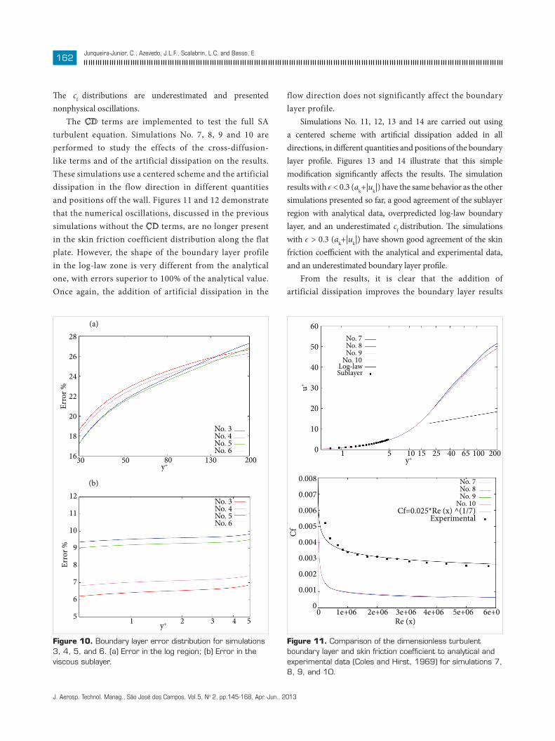
The cf distributions are underestimated and presented nonphysical oscillations.

The CD terms are implemented to test the full SA turbulent equation. Simulations No. 7, 8, 9 and 10 are performed to study the effects of the cross-diffusion-like terms and of the artificial dissipation on the results. These simulations use a centered scheme and the artificial dissipation in the flow direction in different quantities and positions off the wall. Figures 11 and 12 demonstrate that the numerical oscillations, discussed in the previous simulations without the CD terms, are no longer present in the skin friction coefficient distribution along the flat plate. However, the shape of the boundary layer profile in the log-law zone is very different from the analytical one, with errors superior to 100% of the analytical value. Once again, the addition of artificial dissipation in the

flow direction does not significantly affect the boundary layer profile.

Simulations No. 11, 12, 13 and 14 are carried out using a centered scheme with artificial dissipation added in all directions, in different quantities and positions of the boundary layer profile. Figures 13 and 14 illustrate that this simple modification significantly affects the results. The simulation results with ϵ < 0.3 (ak+|uk|) have the same behavior as the other simulations presented so far, a good agreement of the sublayer region with analytical data, overpredicted log-law boundary layer, and an underestimated cf distribution. The simulations with ϵ > 0.3 (ak+|uk|) have shown good agreement of the skin friction coefficient with the analytical and experimental data, and an underestimated boundary layer profile.

From the results, it is clear that the addition of artificial dissipation improves the boundary layer results

28

26

24

22

20

18

16

12

11

10

9

8

7

6

5

Erro

r %Er

ror %

y+

y+



1 2 3 4 5

30 50 80 130 200

(a)

(b)

Figure 10. Boundary layer error distribution for simulations 3, 4, 5, and 6. (a) Error in the log region; (b) Error in the viscous sublayer.

60

50

40

30

20

10

0

0.008

0.007

0.006

0.005

0.004

0.003

0.002

0.001

0

u+

Cf

y+

Re (x)

No. 7No. 8No. 9

No. 10Log-lawSublayer

No. 7No. 8No. 9

No. 10Cf=0.025*Re (x) ^(1/7)

Experimental

1e+06 2e+06 3e+06 4e+06 5e+06 6e+0

1 5 10 15 25 40 65 100 200

0




at the log-law zone, but it deteriorates the viscous sublayer. The implementation of the cross-diffusion-like terms eliminates the numerical oscillations of the cf distribution, but shifts the log-law region of the boundary layer. Using this information, simulations No. 15 to No. 19 are performed using a centered scheme with the addition of artificial dissipation in log-law region and of the CD terms only in the viscous sublayer region of the boundary layer profile. These simulations are performed in order to take advantage of the CD terms near the wall and the artificial dissipation at the log-law zone.

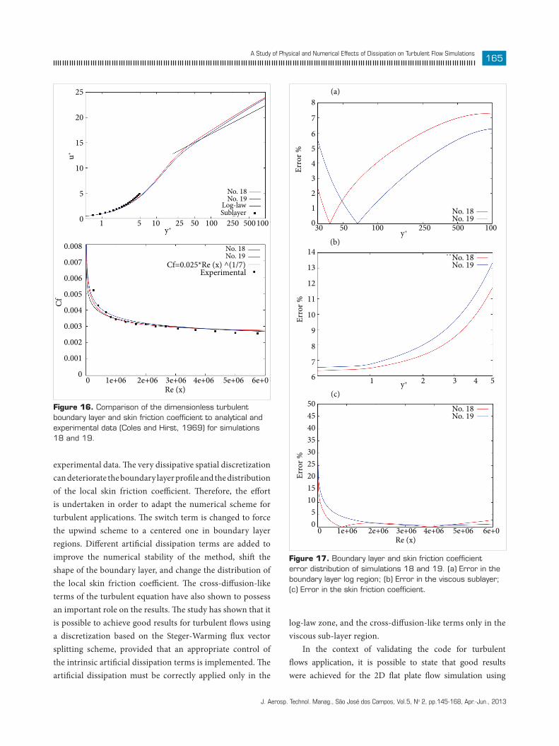
The best results are achieved when the diffusion term, ϵ, is switched off below the viscous sublayer and the CD terms are added only in the viscous sublayer region, as seen in Figs. 15 to 17. Comparing all results, simulations No. 18 and 19 have the best agreement with

the analytical and experimental data, with errors of ≈ 5% for the log-law zone of the boundary layer profile and for the skin friction coefficient distribution over the flat plate. These simulations are carried out using the mesh illustrated in Fig. 7(b). Results are accurate and correspond to aerospace industry needs. On the other hand, the sublayer solutions presented maximum error of ≈10% for the simulations No. 18 and 19. These sublayer errors are not excellent but plausible, since there is good agreement of the log-law zone and the cf distribution with the literature. Therefore, results with good agreement with analytical (von Karman, 1934) and experimental (Coles and Hirst, 1969) data are achieved when one controls the artificial dissipation in the log-law zone, using 1.25 (ak+|uk|) < ϵ < 1.5 (ak+|uk|), and turn off the cross-diffusion-like-terms above the sublayer zone.

180

160

140

120

100

80

60

Erro

r %

12

11

10

9

8

7

6

5

Erro

r %

y+

y+1 2 3 4 5

30 50 80 130 200

No. 7No. 8No. 9

No. 10

No. 7No. 8No. 9

No. 10

(a)

(b)

Figure 12. Boundary layer errors for simulations 7, 8, 9, and 10. (a) Error in the log region; (b) Error in the viscous sublayer.

4540

35

30

25201510

50

0.008

0.007

0.006

0.005

0.004

0.003

0.002

0.001

0

u+C

f

y+

Re (x)

No. 11No. 12No. 13No. 14

Log-lawSublayer

No. 11No. 12No. 13No. 14


1e+06 2e+06 3e+06 4e+06 5e+06 6e+0

1 5 10 15 25 40 65 100 200

0




CONCLUDING REMARKS

Th e present work presents results obtained in the study of the eff ects of artifi cial dissipation terms on the ability of correctly capturing turbulent boundary

layer fl ows. Th e paper presents the details of the theoretical and numerical formulations used. Th e Reynolds-averaged Navier-Stokes equations are used to represent the fl ows of interest here. Turbulent eff ects are modeled using the one-equation Spalart-Allmaras eddy-viscosity turbulent model. Th e work also addresses the inclusion of numerically-stiff cross-diff usion-like (CD) terms in the formulation of the selected turbulence model. Th e work performed included the implementation of the Spalart-Allmaras turbulence closure in the LeMANS code, a parallel CFD code developed to simulate laminar reentry fl ows. Th is code uses a spatial discretization based on the Steger-Warming fl ux vector splitting scheme, which turned out to be very dissipative for boundary layer fl ow applications.

Flat plate zero-pressure-gradient fl ow simulations are performed to evaluate the behavior of the dimensionless boundary layer profi le and to compare with analytical and

140

120

100

80

60

40

20

0

45

40

35

30

25

20

15

10

5

100908070605040302010

0

Erro

r %Er

ror %

Erro

r %

y+

y+

No. 11No. 12No. 13No. 14

No. 11No. 12No. 13No. 14

No. 11No. 12No. 13No. 14

1 2 3 4 5

30 50 80 130 200

Re (x)1e+06 2e+06 3e+06 4e+06 5e+06 6e+00

(a)

(b)

(c)

Figure 14. Boundary layer and skin friction coeffi cient error distribution of simulations 11, 12, 13, and 14. (a) Error in the boundary layer log region; (b) Error in the viscous sublayer; (c) Error in the skin friction coeffi cient.

30

25

20

15

10

5

0

0.008

0.007

0.006

0.005

0.004

0.003

0.002

0.001

0

u+C

f

y+

Re (x)

No. 15No. 16No. 17

No. 15No. 16No. 17

Log-lawSublayer


1e+06 2e+06 3e+06 4e+06 5e+06 6e+0

1 5 10 25 50 100 100250 500

0

Figure 15. Comparison of the dimensionless turbulent boundary layer and skin friction coeffi cient to analytical and experimental data (Coles and Hirst, 1969) for simulations 15, 16, and 17.



experimental data. The very dissipative spatial discretization can deteriorate the boundary layer profile and the distribution of the local skin friction coefficient. Therefore, the effort is undertaken in order to adapt the numerical scheme for turbulent applications. The switch term is changed to force the upwind scheme to a centered one in boundary layer regions. Different artificial dissipation terms are added to improve the numerical stability of the method, shift the shape of the boundary layer, and change the distribution of the local skin friction coefficient. The cross-diffusion-like terms of the turbulent equation have also shown to possess an important role on the results. The study has shown that it is possible to achieve good results for turbulent flows using a discretization based on the Steger-Warming flux vector splitting scheme, provided that an appropriate control of the intrinsic artificial dissipation terms is implemented. The artificial dissipation must be correctly applied only in the

log-law zone, and the cross-diffusion-like terms only in the viscous sub-layer region.

In the context of validating the code for turbulent flows application, it is possible to state that good results were achieved for the 2D flat plate flow simulation using

Erro

r %

14

13

12

11

10

9

8

7

6

8

7

6

5

4

3

2

1

0

504540353025201510

50

Erro

r %Er

ror %

y+

y+

30

1 2 3 4 5

50 100 250 500 100

No. 18No. 19

No. 18No. 19

No. 18No. 19

Re (x)1e+06 2e+06 3e+06 4e+06 5e+06 6e+00

(a)

(b)

(c)

Figure 17. Boundary layer and skin friction coefficient error distribution of simulations 18 and 19. (a) Error in the boundary layer log region; (b) Error in the viscous sublayer; (c) Error in the skin friction coefficient.

25

20

15

10

5

0

0.008

0.007

0.006

0.005

0.004

0.003

0.002

0.001

0

u+

Cf

y+

Re (x)

No. 18No. 19

No. 18No. 19

Log-lawSublayer


1e+06 2e+06 3e+06 4e+06 5e+06 6e+0

1 5 10 25 50 100 100250 500

0

Figure 16. Comparison of the dimensionless turbulent boundary layer and skin friction coefficient to analytical and experimental data (Coles and Hirst, 1969) for simulations 18 and 19.



spatial discretization based on the Steger-Warming scheme. However, the good agreement is dependent upon the addition of artificial dissipation and CD terms at the correct position in the boundary layer profile. In the present work, these modifications are explicitly performed to provide good results for a predefined local Reynolds number. It is very important to adapt the switches in the computational implementation of the numerical scheme in order to add artificial dissipation in the correct position in the boundary layer profile. Similarly, the cross-diffusion-like terms must be switched on only in the sublayer region. Hence, the turbulence model implementation must be performed in such a way that the code could automatically recognize the correct position in the dimensionless boundary layer profile and switch on/off the CD terms and the artificial dissipation. This can certainly be accomplished using an appropriate scaling of boundary layer quantities and the normalized distance to the wall, which is already computed by the turbulence model. However, these are implementation issues, which are beyond the scope of

the present work. Clearly, such implementations would be necessary in order to handle more complex configurations. More complex applications, in the sense, for instance, of treating flows with more obvious compressibility effects, are not an issue, since the turbulence model and the present CFD tool were both originally developed for compressible flows.

ACKNOWLEDGMENTS

The authors would like to acknowledge Conselho Nacional de Desenvolvimento Científico e Tecnológico, CNPq, which partially supported the project under the Research Grants No. 312064/2006-3 and No. 471592/2011-0. Further partial support was provided by Fundação Coordenação de Aperfeiçoamento Pessoal de Nível Superior, CAPES, through a Ph.D. scholarship to the first author, and it is also gratefully acknowledged.

REFERENCES

Anderson, J.D., 1991, “Fundamentals of Aerodynamics”, McGraw-Hill International Editions, New York, NY, USA.

Anderson, W.K., Thomas, J.L. and van Leer, B., 1986, “A Comparison Of Finite Volume Flux Vector Splittings For The Euler Equations”, AIAA Journal, Vol. 24, No. 9, pp. 1453-1460.

Azevedo, J.L.F., 1988, “Transonic Aeroelastic Analysis Of Launch Vehicle Configurations”, Ph.D. Thesis, Stanford University, Stanford, California, USA.

Basso, E., 1997, “Numerical Analysis of Cascade Flow Problems for All Speed Regimes”, Master’s Thesis, Instituto Tecnológico de Aeronáutica, São José dos Campos, SP, Brazil (in Portuguese, original title is Análise Numérica de Escoamentos em Grades Lineares de Perfis para Vários Regimes de Velocidade).

Batina, J., 1990, “Three-Dimensional Flux-Split Euler Schemes Involving Unstructured Dynamic Meshes”, AIAA Paper No. 90-1649, 21st AIAA Fluid Dynamics, Plasma Dynamics and Lasers Conference, Seattle, WA.

Batten, P., Craft, T.J., Leschziner, M.A. and Loyau, H., 1999, “Reynolds-Stress-Transport Modeling for Compressible Aerodynamics Applications”, AIAA Journal, Vol. 37, No. 7, pp. 785-797.

Bibb, K.L., Peraire, J. and Riley, C.J., 1997, “Hypersonic Flow Computations On Unstructured Meshes”, AIAA Paper No. 97-0625.

Bigarella, E.D.V., 2007, “Advanced Turbulence Modeling for Complex Aerospace Applications”, Ph.D. Thesis, Instituto Tecnológico de Aeronáutica, São José dos Campos, SP, Brazil.

Bigarella, E.D.V. and Azevedo, J.L.F., 2009, “Turbulence Modeling for Aerospace Applications, Turbulence”, Vol. 6 of Coleção Cadernos de Turbulência, Chapter 4, ABCM, Rio de Janeiro, RJ, 1st ed., pp. 215-296 (in Portuguese, original title is Modelagem de Turbulência para Aplicações Aeroespaciais).

Bigarella, E.D.V. and Azevedo, J.L.F., 2012, “A Study Of Convective Flux Schemes For Aerospace Flows”, Journal of the Brazilian Society for Mechanical Sciences and Engineering, Vol. 34, No. 3, pp. 314-329.

Bigarella, E.D.V., Azevedo, J.L.F. and Scalabrin, L.C., 2007, “Centered and Upwind Multigrid Turbulent Flow Simulations of Launch Vehicle Configurations”, Journal of Spacecraft and Rockets, Vol. 44, No. 1, pp. 52-65.

Breviglieri, C., 2010, “High-Order Unstructured Spectral Finite Volume Method for Aerodynamic Applications”, Master’s Thesis, Instituto Tecnológico de Aeronáutica, São José dos Campos, SP, Brazil.

Breviglieri, C., Azevedo, J.L.F. and Basso, E., 2010a, “An Unstructured Grid Implementation Of High-Order Spectral Finite Volume Schemes”, Journal of the Brazilian Society of Mechanical Sciences and Engineering, Vol. 32, No. 5 (Special Issue), pp. 419-433.

Breviglieri, C., Azevedo, J.L.F., Basso, E. and Souza, M.A.F., 2010b, “Implicit High-Order Spectral Finite Volume Method For Inviscid Compressible Flows”, AIAA Journal, Vol. 48, No. 10, pp. 2365-2376.

Chapman, D., 1981, “Trends and Pacing Items in Computational Aerodynamics, Seventh International Conference on Numerical



Methods in Fluid Dynamics”, edited by W. Reynolds and R. MacCormack, Lecture Notes in Physics, Vol. 141, Springer, Heidelberg, pp. 1–11.

Coles, D.E. and Hirst, E.A., 1969, “Computation Of Turbulent Boundary Layers”, Proceedings of the 1968 U.S. Air Force Office of Scientific Research-Internal Flow Program-Stanford Conference, Vol. 2, Stanford University Press, Palo Alto, CA, USA.

Gnoffo, P.A., 2003, “Computational Aerothermodynamics In Aeroassist Applications”, Journal of Spacecraft and Rockets, Vol. 40, No. 3, pp. 305-312.

Hellsten, A. and Laine, S., 2000, “Explicit Algebraic Reynolds-Stress Modelling In Decelerating And Separating Flows”, AIAA Paper No. 2000-2313.

Hirsch, C., 1990, “Numerical Computation of Internal and External Flows, Vol. II: Computational Methods for Inviscid and Viscous Flows”, Wiley, New York, USA.

Jameson, A., 1995a, “Analysis And Design Of Numerical Schemes For Gas Dynamics 1 – Artificial Diffusion, Upwind Biasing, Limiters And Their Effect On Accuracy And Multigrid Convergence”, International Journal of Computational Dynamics, Vol. 4, No. 3-4, pp. 171-218.

Jameson, A., 1995b, “Analysis And Design Of Numerical Schemes For Gas Dynamics 2 – Artificial Diffusion And Discrete Shock Structure”, International Journal of Computational Dynamics, Vol. 5, No. 1-2, pp. 1-38.

Jameson, A., Schmidt, W. and Turkel, E., 1981, “Numerical Solution Of The Euler Equations By Finite Volume Methods Using Runge-Kutta Time-Stepping Schemes”, AIAA Paper No. 81-1259.

Jawahar, P. and Kamath, H., 2000, “A High Resolution Procedure For Euler And Navier-Stokes Computation On Unstructured Grids”, Journal of Computational Physics, Vol. 164, No. 1, pp. 165-203.

Junqueira-Junior, C.A., 2012, “A Study On The Extension Of An Upwind Parallel Solver For Turbulent Flow Applications”, Master’s Thesis, Instituto Tecnológico de Aeronáutica, São José dos Campos, São Paulo, Brazil.

Junqueira-Junior, C.A., Azevedo, J.L.F., Basso, E. and Scalabrin, L., 2011, “Study Of Robust And Efficient Turbulence Closures For Aerospace Applications”, 32nd Iberian Latin American Congress on Computational Methods in Engineering, Ouro Preto, Minas Gerais, Brazil.

Lomax, H., Pulliam, T.H. and Zingg, D.W., 2001, “Fundamentals of Computation Fluid Dynamics”, Springer, New York, USA.

Long, L.N., Khan, M. and Sharp, H.T. 1991, “A Massively Parallel Three-Dimensional Euler/Navier-Stokes Method”, AIAA Journal, Vol. 29, No. 5, pp. 657-666.

MacCormack, R.W. and Candler, G.V., 1989, “The Solution of the Navier Stokes Equations Using Gauss-Seidel Line Relaxation”, Computer and Fluids, Vol. 17, No. 1, pp. 135-150.

Mavriplis, D.J., 1988, “Accurate Multigrid Solution of the Euler Equations on Unstructured and Adaptive Meshes”, AIAA Journal, Vol. 28, No. 2, pp. 213-221.

Ramalho, M.V.C., Azevedo, J.H.A. and Azevedo, J.L.F., 2011, “Further Investigation into the Origin of the Carbuncle Phenomenon in Aerodynamic Simulations”, AIAA Paper No. 2011-1184, 49th AIAA Aerospace Sciences Meeting including the New Horizons Forum and Aerospace Exposition, Orlando, Florida, USA.

Roe, P.L., 1981, “Approximate Riemann Solvers, Parameter Vectors, and Difference Schemes”, Journal of Computational Physics, Vol. 43, No. 2, pp. 357-372.

Scalabrin, L.C., 2007, “Numerical Simulation of Weakly Ionized Hypersonic Flow Over Reentry Capsules”, Ph.D. Thesis, University of Michigan, Ann Arbor, Michigan, USA.

Scalabrin, L.C. and Boyd, I.D., 2007, “Numerical Simulations of the FIRE-II Convective and Radiative Heating Rates”, AIAA Paper No. 2007-4044.

Schlichting, H., 1978, “Boundary-Layer Theory”, 7th ed., McGraw Hill, New York, NY, USA.

Schwartzentruber, T.E., Scalabrin, L.C. and Boyd, I.D., 2007, “A Modular Particle-Continuum Numerical Method For Hypersonic Non-Equilibrium Gas Flows”, Journal of Computational Physics, Vol. 225, No. 1, pp. 1159-1174.

Schwartzentruber, T.E., Scalabrin, L.C. and Boyd, I.D., 2008, “Hybrid Particle-Continuum Simulations Of Non-Equilibrium Hypersonic Blunt-Body Flowfields”, Journal of Thermophysics and Heat Transfer, Vol. 22, No. 1, pp. 29-37.

Spalart, P.R. and Allmaras, S.R., 1992, “A One-Equation Turbulence Model For Aerodynamic Flows”, AIAA Paper No. 92-0439.

Spalart, P.R. and Allmaras, S.R., 1994, “A One-Equation Turbulence Model For Aerodynamic Flows”, La Recherche Aerospatiale, Vol. 1, No. 1, pp. 5-21.

Steger, J.L. and Warming, R.F., 1981, “Flux Vector Splitting of the Inviscid Gasdynamic Equations with Application to the Finite-Difference Method”, Journal of Computational Physics, Vol. 40, No. 2, pp. 263-293.

Tennekes, H. and Lumley, J.L., 1972, “A First Course In Turbulence”, The MIT Press, Cambridge, MA, USA.

Turkel, E. and Vatsa, V.N., 1990, “Effect of Artificial Viscosity on Three-Dimensional Flow Solutions”, AIAA Journal, Vol. 32, No. 1, pp. 39-45.

van Albada, G.D., 1982, van Leer, B. and Roberts, W.W., 1982, “A Comparative Study of Computational Methods in Cosmic Gas Dynamics”, Astronomy and Astrophysics, Vol. 108, No. 1, pp. 76-84.

van der Burg, J.W. 2000, “Turnaround Time And Accuracy Evaluation Of Viscous Flow Computations On Hybrid Grids”, Technical Report NLR-TP-2000-228, Amsterdam, The Netherlands.

van Leer, B., 1979, “Towards the Ultimate Conservative Difference Scheme. V. A Second-Order Sequel to Godunov’s Method”, Journal of Computational Physics, Vol. 32, No. 1, pp. 101-136.

Venkatakrishnan, V., 1995, “Implicit Schemes and Parallel Computing in Unstructured Grid CFD”, VKI Lecture Series, Rhode-Saint-Genèse, Belgium.

von Karman, T., 1934, “Turbulence and Skin Friction”, Journal of the Aeronautical Sciences, Vol. 1, No. 1, pp. 1-20.

Wallin, S. and Johansson, A.V., 2000, “An Explicit Algebraic Reynolds Stress Model For Incompressible And Compressible Turbulent Flows”, Journal of Fluid Mechanics, Vol. 403, pp. 89-132.

Wolf, W.R., 2006, “Simulation of Compressible Aerodynamic Flows Using Unstructured Grid, High-Order, Non-Oscillatory Schemes”, Master’s Thesis, Instituto Tecnológico de Aeronáutica, São José



dos Campos, SP, Brazil (in Portuguese, original title is Simulação de Escoamentos Aerodinâmicos Compressíveis Utilizando Esquemas Não Oscilatórios de Alta Ordem de Precisão em Malhas Não Estruturadas).

Wolf, W.R. and Azevedo, J.L.F., 2006, “High-Order Unstructured Essentially Nonoscillatory and Weighted Essentially Nonoscillatory Schemes for Aerodynamic Flows”, AIAA Journal, Vol. 44, No. 10, pp. 2295-2310.

Wolf, W.R. and Azevedo, J.L.F., 2007, “High-Order ENO and WENO Schemes for Unstructured Grids”, International Journal for Numerical Methods in Fluids, Vol. 55, No. 10, pp. 917-943.

Wright, M.J., 1997, “A Family of Data Parallel Relaxation Methods for the Navier-Stokes Equations”, Ph.D. Thesis, University of Minnesota, Minneapolis, MN, USA.

Documents

A Study of Physical and Numerical Effects of Dissipation ... · studying the effects of artificial dissipation and of certain diffusive ... high lift and drag ... work is to take