Implementation of Wave Dissipation by Vegetation in STWAVE · Implementation of Wave Dissipation by Vegetation in STWAVE ... Implementation of Wave Dissipation by Vegetation in

ERDC/CHL CHETN-I-85 February 2015

Approved for public release; distribution is unlimited.

Implementation of Wave Dissipation

by Vegetation in STWAVE

by Mary E. Anderson and Jane McKee Smith

PURPOSE: This Coastal and Hydraulics Engineering Technical Note (CHETN) describes the implementation of wave dissipation by vegetation into the nearshore spectral wave model STWAVE (Massey et al. 2011; Smith 2007; Smith et al. 2001).

INTRODUCTION: The influence of vegetation on coastal hydrodynamics is a relatively new field, with a body of literature documenting the dissipation of wave energy by coastal vegetation developing within the last few decades (see Anderson et al. (2011) for a summary). Unfortunately, the effect of vegetation on coastal processes and hydrodynamics is not fully implemented in many numerical models. Standard practice in nearshore wave propagation models, including STWAVE and SWAN, is to account for energy losses due to vegetation using bottom friction source terms. The need to accurately predict coastal hydrodynamics in the presence of natural or nature-based features has led to an increasing demand for models that better capture wave interaction with vegetation. Compounded by a lack of technique and guidance, the beneficial effects of vegetation are often neglected in the analysis, design, and construction of coastal protection.

Theoretical models for estimating wave dissipation based on energy conservation were initially proposed for monochromatic waves (Dalrymple et al. 1984), with later expansions to narrow-banded random waves (Mendez and Losada 2004). One noticeable improvement over the current bottom friction formulations is the capability to describe the vegetation itself. The declared vegetation characteristics are the following: vegetation height, stem diameter, vegetation density, and a bulk drag coefficient calibrated for the specific plant type and hydrodynamic conditions. Calibration of this bulk drag coefficient accounts for many processes not yet fully understood, such as plant motion. The study of its behavior with respect to wave attenuation is currently ongoing. The random wave dissipation model proposed by Mendez and Losada (2004) is the most appropriate for inclusion into STWAVE due to its reasonable representation of the physical processes and feasibility to implement.

FORMULATION: Waves propagating through vegetation dissipate energy due to the work carried out on the vegetation. Assuming the validity of linear wave theory, the conservation of energy is as follows:

gv

ECε

x

where E is wave energy, Cg is group velocity, x is the horizontal distance over which the wave travels, and εv is the time-averaged rate of energy dissipation due to vegetation per unit horizontal area. Integrating vertically over the vegetation height (ls) and assuming εv is only a function of the

Report Documentation Page Form ApprovedOMB No. 0704-0188

Public reporting burden for the collection of information is estimated to average 1 hour per response, including the time for reviewing instructions, searching existing data sources, gathering andmaintaining the data needed, and completing and reviewing the collection of information. Send comments regarding this burden estimate or any other aspect of this collection of information,including suggestions for reducing this burden, to Washington Headquarters Services, Directorate for Information Operations and Reports, 1215 Jefferson Davis Highway, Suite 1204, ArlingtonVA 22202-4302. Respondents should be aware that notwithstanding any other provision of law, no person shall be subject to a penalty for failing to comply with a collection of information if itdoes not display a currently valid OMB control number.

1. REPORT DATE FEB 2015 2. REPORT TYPE

3. DATES COVERED 00-00-2015 to 00-00-2015

4. TITLE AND SUBTITLE Implementation of Wave Dissipation by Vegetation in STWAVE

5a. CONTRACT NUMBER

5b. GRANT NUMBER

5c. PROGRAM ELEMENT NUMBER

6. AUTHOR(S) 5d. PROJECT NUMBER

5e. TASK NUMBER

5f. WORK UNIT NUMBER

7. PERFORMING ORGANIZATION NAME(S) AND ADDRESS(ES) U.S. Army Engineer Research and Development Center,(ERDC), Coastaland Hydraulics Laboratory (CHL),,Vicksburg,,MS

8. PERFORMING ORGANIZATIONREPORT NUMBER

9. SPONSORING/MONITORING AGENCY NAME(S) AND ADDRESS(ES) 10. SPONSOR/MONITOR’S ACRONYM(S)

11. SPONSOR/MONITOR’S REPORT NUMBER(S)

12. DISTRIBUTION/AVAILABILITY STATEMENT Approved for public release; distribution unlimited

13. SUPPLEMENTARY NOTES

14. ABSTRACT

15. SUBJECT TERMS

16. SECURITY CLASSIFICATION OF: 17. LIMITATION OF ABSTRACT Same as

Report (SAR)

18. NUMBEROF PAGES

17

19a. NAME OFRESPONSIBLE PERSON

a. REPORT unclassified

b. ABSTRACT unclassified

c. THIS PAGE unclassified

Standard Form 298 (Rev. 8-98) Prescribed by ANSI Std Z39-18


2

horizontal drag force (inertial component neglected), the definition for the depth-integrated and time-averaged energy dissipation per horizontal area for a vegetation field is given by

sd l

v xdε F udz

where d is water depth and z is the vertical dimension. The horizontal force per unit volume (Fx) is described using a Morison-type equation (Morison et al. 1950):

x D vF ρC b Nu u12

where ρ is the density of water, C̃D is a depth-averaged drag coefficient, bv is stem diameter, N is vegetation density, and u is the horizontal fluid velocity due to wave motion.

Mendez and Losada (2004) modified the Dalrymple et al. (1984) formulation by using a Rayleigh distribution to describe the variation in wave height, yielding the following for random waves:

sinh sinhcoshs s

v D v rmskl klkgε ρC b N H

ω k kdπ

3 33

3

312 32

where g is the acceleration due to gravity, k is wave number, ω is wave angular frequency, Hrms is root-mean-square wave height, and CD is an average or bulk depth-averaged drag coefficient that is dependent on hydrodynamic and plant characteristics.

The STWAVE source term for wave damping due to vegetation (Sveg) is obtained by expanding the Mendez and Losada (2004) formulation for εv to include frequencies and directions (Suzuki et al. 2011):

sinh sinhω,

coshs s

veg D v totl kl

S g C b N E E θπ k d

kkω k

3 32

3

323

in which k is the mean wave number, ω is the mean angular frequency, and Etot is the total wave energy. When the vegetation height exceeds the water depth (ls > d), the vegetation height is dynamically set equal to the water depth (ls = d) within STWAVE.

MODEL INPUT. The primary input file for STWAVE is the simulation file (*.sim), and it is within this file that model controls are defined through a series of FORTRAN namelists that specify parameters and run options. For a detailed description, see the STWAVE v6.0 user’s manual (Massey et al. 2011). To implement vegetation dissipation into STWAVE, an additional model option IVEG was required in the std_parms namelist. A description of the IVEG option is provided below.

IVEG = Flag to exclude vegetation (IVEG = 0, default option) or include vegetation (IVEG = 1 or 2). Spatially constant vegetation (IVEG = 1) requires specification of vegetation


3

parameters within the simulation file while spatially variable vegetation (IVEG = 2) requires an input file that specifies the vegetation parameters for every grid cell. The vegetation parameters required for both options are the following: average vegetation height, average stem diameter, number of plants per unit horizontal area, and bulk drag coefficient.

To accommodate the spatially constant vegetation option (IVEG = 1), a new namelist was added called const_veg. The vegetation parameters for the IVEG = 1 option must be defined within the const_veg namelist in the *.sim file. As a reminder, all FORTRAN namelists start with the ampersand symbol (&), followed by the namelist name. Variables assigned to the namelist are then listed along with the assigned value. The end of the namelist is indicated by the slash symbol (/). The const_veg namelist must be specified before the optional namelists, which are indicated by the symbol @ in the STWAVE *.sim file. The required model parameters for the new const_veg namelist are provided in Table 1.

Table 1. Model parameters: Spatially constant vegetation – const_veg namelist. Parameter Type Definition veg_ls_const real number # = average vegetation height [m] veg_bv_const real number # = average stem diameter [m] veg_N_const real number # = vegetation density [stems/m2] veg_Cd_const real number # = bulk drag coefficient [-]

For the spatially variable vegetation option (IVEG = 2), vegetation parameters for each grid cell are defined using an external input file. The external input filename is specified under the input_file namelist in the *.sim file using the VEG option. The values must be provided in column format, with the following parameters from left to right: average vegetation height, average stem diameter, vegetation density, and bulk drag coefficient. The format is the same as the other global STWAVE files and is read using the following FORTRAN algorithm:

do j = NJ, 1, -1 do i = 1, NI read (10, *) veg_ls(i,j), veg_bv(i,j), veg_N(i,j), veg_Cd(i,j) enddo enddo

Excerpts of the required changes to the STWAVE simulation file for spatially constant vegetation (IVEG = 1) and spatially variable vegetation (IVEG = 2) are highlighted in Appendix A. An example of the external input file required for spatially variable vegetation (IVEG = 2) is provided in Appendix B.

MODEL VALIDATION

Mendez and Losada (2004). Comparisons of STWAVE to the analytical dissipation model of Mendez and Losada (2004) were completed to confirm correct implementation of the source term. The random wave transformation model for a flat bottom was proposed by Mendez and Losada (2004) as


4

,rmsrms

HH

βx

0

1

with

,

sinh sinhsinh sinh

s sD v rms

kl klβ C b NH k

kd kd kdπ

3

031

2 23

where Hrms,0 is the root-mean-square wave height incident to the vegetation (x = 0). The root-mean-square wave height is related to the significant wave height (Hmo) by

morms

HH

2

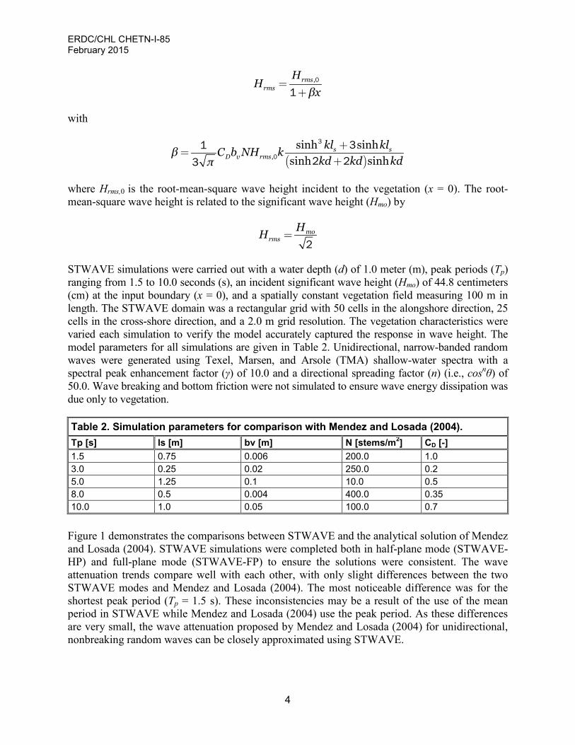
STWAVE simulations were carried out with a water depth (d) of 1.0 meter (m), peak periods (Tp) ranging from 1.5 to 10.0 seconds (s), an incident significant wave height (Hmo) of 44.8 centimeters (cm) at the input boundary (x = 0), and a spatially constant vegetation field measuring 100 m in length. The STWAVE domain was a rectangular grid with 50 cells in the alongshore direction, 25 cells in the cross-shore direction, and a 2.0 m grid resolution. The vegetation characteristics were varied each simulation to verify the model accurately captured the response in wave height. The model parameters for all simulations are given in Table 2. Unidirectional, narrow-banded random waves were generated using Texel, Marsen, and Arsole (TMA) shallow-water spectra with a spectral peak enhancement factor (γ) of 10.0 and a directional spreading factor (n) (i.e., cosnθ) of 50.0. Wave breaking and bottom friction were not simulated to ensure wave energy dissipation was due only to vegetation.

Table 2. Simulation parameters for comparison with Mendez and Losada (2004). Tp [s] ls [m] bv [m] N [stems/m2] CD [-] 1.5 0.75 0.006 200.0 1.0 3.0 0.25 0.02 250.0 0.2 5.0 1.25 0.1 10.0 0.5 8.0 0.5 0.004 400.0 0.35 10.0 1.0 0.05 100.0 0.7

Figure 1 demonstrates the comparisons between STWAVE and the analytical solution of Mendez and Losada (2004). STWAVE simulations were completed both in half-plane mode (STWAVE-HP) and full-plane mode (STWAVE-FP) to ensure the solutions were consistent. The wave attenuation trends compare well with each other, with only slight differences between the two STWAVE modes and Mendez and Losada (2004). The most noticeable difference was for the shortest peak period (Tp = 1.5 s). These inconsistencies may be a result of the use of the mean period in STWAVE while Mendez and Losada (2004) use the peak period. As these differences are very small, the wave attenuation proposed by Mendez and Losada (2004) for unidirectional, nonbreaking random waves can be closely approximated using STWAVE.


5

Figure 1. Comparisons of wave height evolution between STWAVE and Mendez

and Losada (2004).

T = 1.5 s T = 3.0 s 0.5

p p 0.5

0.4 Mendez and Losada (2004) 0.4

E 0.3 E 0.3

0 0 E E

I 0.2 I 0.2

0.1 0.1

0 0 0 20 40 60 80 100 0 20 40 60 80 100

x[m] x[m]

T = 5.0 s T = 8.0 s 0.5

p 0.5

p

0.4 0.4

.s 0.3 E 0.3

0 0 E E

I 0.2 I 0.2

0.1 0.1

0 0 0 20 40 60 80 100 0 20 40 60 80 100

x[m] x[m] T = 10.0 s

0.5 p

0.4

E 0.3

0 E

I 0.2

0.1

0 0 20 40 60 80 100

x[m]


6

SENSITVITY TO SPECTRAL PARAMETERS

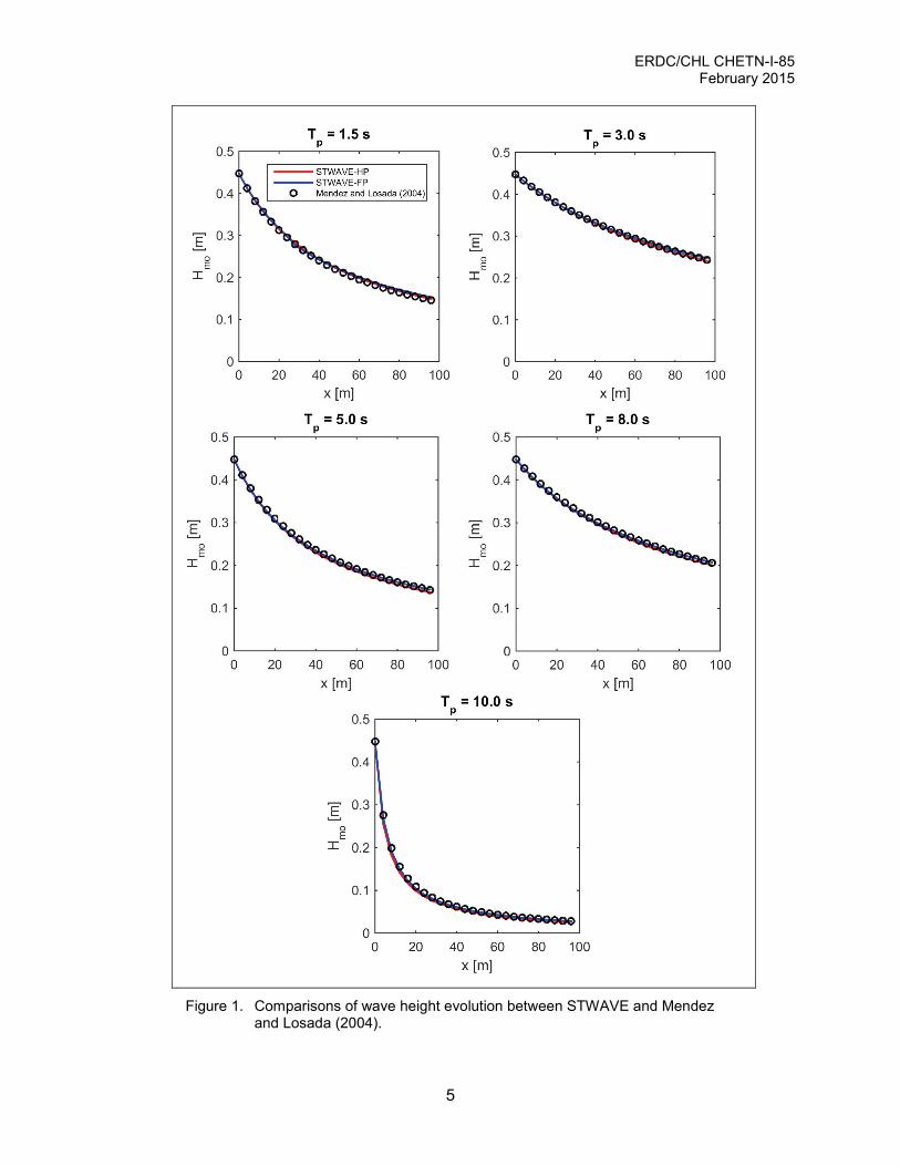
Frequency. The sensitivity of the STWAVE solution to differences in the peak enhancement factor (γ) is investigated by comparing TMA spectra of γ = 10.0, considered a narrow spectral value, and γ = 3.3, a common default value. An illustration of the resulting difference in spectral shape is provided in Figure 2. A larger peak enhancement factor (γ) results in a narrower and greater concentration of energy at the peak frequency compared to smaller γ values.

Figure 2. TMA spectra with γ = 10.0

and γ = 3.3 for Tp = 3.0 s.

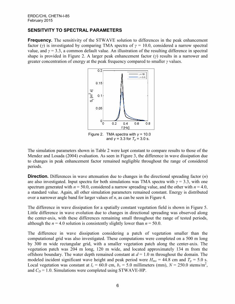
The simulation parameters shown in Table 2 were kept constant to compare results to those of the Mendez and Losada (2004) evaluation. As seen in Figure 3, the difference in wave dissipation due to changes in peak enhancement factor remained negligible throughout the range of considered periods.

Direction. Differences in wave attenuation due to changes in the directional spreading factor (n) are also investigated. Input spectra for both simulations was TMA spectra with γ = 3.3, with one spectrum generated with n = 50.0, considered a narrow spreading value, and the other with n = 4.0, a standard value. Again, all other simulation parameters remained constant. Energy is distributed over a narrower angle band for larger values of n, as can be seen in Figure 4.

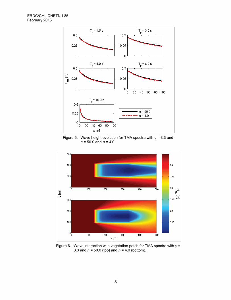
The difference in wave dissipation for a spatially constant vegetation field is shown in Figure 5. Little difference in wave evolution due to changes in directional spreading was observed along the center-axis, with these differences remaining small throughout the range of tested periods, although the n = 4.0 solution is consistently slightly lower than n = 50.0.

The difference in wave dissipation considering a patch of vegetation smaller than the computational grid was also investigated. These computations were completed on a 500 m long by 300 m wide rectangular grid, with a smaller vegetation patch along the center-axis. The vegetation patch was 204 m long, 120 m wide, and located approximately 134 m from the offshore boundary. The water depth remained constant at d = 1.0 m throughout the domain. The modeled incident significant wave height and peak period were Hmo = 44.8 cm and Tp = 5.0 s. Local vegetation was constant at ls = 60.0 cm, bv = 5.0 millimeters (mm), N = 250.0 stems/m2, and CD = 1.0. Simulations were completed using STWAVE-HP.


7

Figure 3. Wave height evolution for TMA spectra with γ = 10.0

and γ = 3.3 and n = 50.0.

Figure 4. TMA spectra with n = 50.0 and n = 4.0 for Tp = 5.0 s.

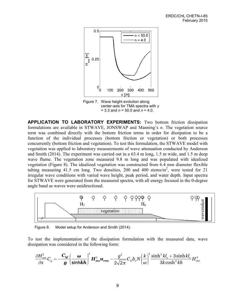
Figure 6 and Figure 7 show that the most noticeable difference in wave height is located downstream of the vegetation patch. Reduced wave height is seen behind the patch for n = 50.0 as the waves are impeded and limited in direction. However, waves are able to propagate and reform downstream of the vegetation for n = 4.0 as wave energy is distributed amongst a broader range of directions. This wave behavior is similar to that observed for irregular wave interactions with structures.


8

Figure 5. Wave height evolution for TMA spectra with γ = 3.3 and

n = 50.0 and n = 4.0.

Figure 6. Wave interaction with vegetation patch for TMA spectra with γ =

3.3 and n = 50.0 (top) and n = 4.0 (bottom).


9

Figure 7. Wave height evolution along

center-axis for TMA spectra with γ = 3.3 and n = 50.0 and n = 4.0.

APPLICATION TO LABORATORY EXPERIMENTS: Two bottom friction dissipation formulations are available in STWAVE, JONSWAP and Manning’s n. The vegetation source term was combined directly with the bottom friction terms in order for dissipation to be a function of the individual processes (bottom friction or vegetation) or both processes concurrently (bottom friction and vegetation). To test this formulation, the STWAVE model with vegetation was applied to laboratory measurements of wave attenuation conducted by Anderson and Smith (2014). The experiment was carried out in a 63.4 m long, 1.5 m wide, and 1.5 m deep wave flume. The vegetation zone measured 9.8 m long and was populated with idealized vegetation (Figure 8). The idealized vegetation was constructed from 6.4 mm diameter flexible tubing measuring 41.5 cm long. Two densities, 200 and 400 stems/m2, were tested for 21 irregular wave conditions with varied wave height, peak period, and water depth. Input spectra for STWAVE were generated from the measured spectra, with all energy focused in the 0-degree angle band as waves were unidirectional.

Figure 8. Model setup for Anderson and Smith (2014).

To test the implementation of the dissipation formulation with the measured data, wave dissipation was considered in the following form:

sinh sinhcosh

mo s sg D v mo

H kl klg kC C b N Hx ω k khπ

sinh

2 32 322 3

3

332 2

bfmo rms

C ω H ug kh


10

where the first term on the right-hand side of the equation, shown in bold, is the Manning’s n bottom friction source term, and the second term is the vegetation source term. The background dissipation due to friction in the flume (Cbf), was first solved for by assuming no vegetation:

sinhln

Δg

bfrms

CH g khCH u ω x

22220

where the root-mean-square horizontal wave velocity (urms), was defined at the bottom and was calculated as

sinhrms

H ωukh

0

2 2

Cbf was calculated using the unimpeded control runs (no vegetation), with Hmo measured at the gauge immediately incident to the vegetation test section and at the last gauge corresponding to H0 and H2, respectively. The location of these gauges of interest is identified in Figure 8.

After estimating the background friction, the drag coefficient due to vegetation was estimated:

Δlnsinh

sinh sinh Δcosh

bfrms

gD

s sv

g

CH ω xuH g kh C

Ckl klg k xb N H

ω k kh Cπ

22220

3 32

13

332 2

Again, H0 is measured at the gauge immediately upstream of the vegetation test section, and H2 is measured at the last gauge (downstream end). The input into STWAVE, Manning’s n, was obtained by rearranging Cbf:

/

bfbf

C hn

g

1 3

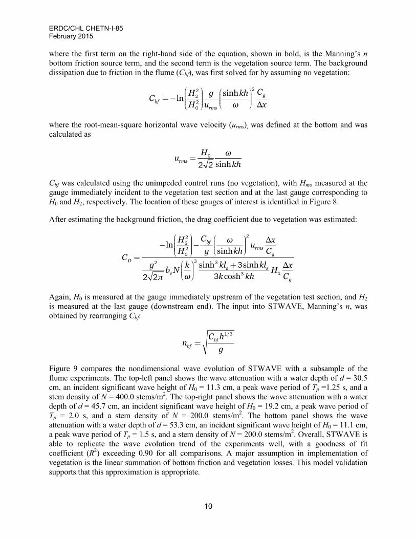
Figure 9 compares the nondimensional wave evolution of STWAVE with a subsample of the flume experiments. The top-left panel shows the wave attenuation with a water depth of d = 30.5 cm, an incident significant wave height of H0 = 11.3 cm, a peak wave period of Tp =1.25 s, and a stem density of N = 400.0 stems/m2. The top-right panel shows the wave attenuation with a water depth of d = 45.7 cm, an incident significant wave height of H0 = 19.2 cm, a peak wave period of Tp = 2.0 s, and a stem density of N = 200.0 stems/m2. The bottom panel shows the wave attenuation with a water depth of d = 53.3 cm, an incident significant wave height of H0 = 11.1 cm, a peak wave period of Tp = 1.5 s, and a stem density of N = 200.0 stems/m2. Overall, STWAVE is able to replicate the wave evolution trend of the experiments well, with a goodness of fit coefficient (R2) exceeding 0.90 for all comparisons. A major assumption in implementation of vegetation is the linear summation of bottom friction and vegetation losses. This model validation supports that this approximation is appropriate.


11

Figure 9. Wave height comparisons of STWAVE and the laboratory results of

Anderson and Smith (2014): (top left) d = 30.5 cm, H0 = 11.3 cm, Tp = 1.25 s, N = 400.0 stems/m2; (top right) d = 45.7 cm, H0 = 19.2 cm, Tp = 2.0 s, N = 200.0 stems/m2; (bottom) d = 53.3 cm, H0 = 11.1 cm, Tp = 1.5 s, N = 200.0 stems/m2.

CONCLUSIONS: The analysis, design, and construction of coastal protection often neglect the beneficial effects of natural or nature-based features because insufficient methods are available to capture those benefits. In this technical note, random wave dissipation by vegetation is implemented into the phase-averaged nearshore wave model STWAVE. The vegetation dissipation source term is first validated by comparing model results to the solution of Mendez and Losada (2004) for unidirectional, nonbreaking waves. Following validation, the sensitivity of the model solution to energy distribution in frequency and direction is investigated. The difference in wave height as a result of frequency spread was minute for the range of considered periods. The wave height evolution along the center line of a domain with spatially constant vegetation was also insensitive to differences in directional spreading. However, the global wave solution changes considerably with directional spreading when considering a local vegetation patch, particularly downstream of the vegetation. Finally, combining the vegetation source term with the already existing bottom friction terms in STWAVE was tested using the flume experiments of Anderson and Smith (2014). By first solving for the bottom friction coefficient and then the bulk drag coefficient, a good prediction of wave dissipation was obtained. Since the bulk drag coefficient accounts for many assumptions and processes not yet fully understood,


12

calibration of the bulk drag coefficient is essential to obtain accurate results, and its dependence on hydrodynamics and plant biomechanics requires additional investigation.

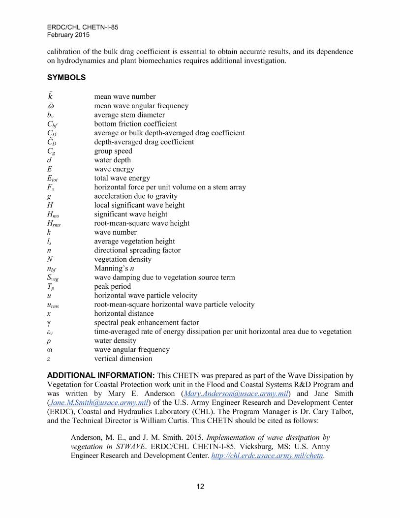
SYMBOLS

k mean wave number ω mean wave angular frequency bv average stem diameter Cbf bottom friction coefficient CD average or bulk depth-averaged drag coefficient C̃D depth-averaged drag coefficient Cg group speed d water depth E wave energy Etot total wave energy Fx horizontal force per unit volume on a stem array g acceleration due to gravity H local significant wave height Hmo significant wave height Hrms root-mean-square wave height k wave number ls average vegetation height n directional spreading factor N vegetation density nbf Manning’s n Sveg wave damping due to vegetation source term Tp peak period u horizontal wave particle velocity urms root-mean-square horizontal wave particle velocity x horizontal distance γ spectral peak enhancement factor εv time-averaged rate of energy dissipation per unit horizontal area due to vegetation ρ water density ω wave angular frequency z vertical dimension

ADDITIONAL INFORMATION: This CHETN was prepared as part of the Wave Dissipation by Vegetation for Coastal Protection work unit in the Flood and Coastal Systems R&D Program and was written by Mary E. Anderson ([email protected]) and Jane Smith ([email protected]) of the U.S. Army Engineer Research and Development Center (ERDC), Coastal and Hydraulics Laboratory (CHL). The Program Manager is Dr. Cary Talbot, and the Technical Director is William Curtis. This CHETN should be cited as follows:

Anderson, M. E., and J. M. Smith. 2015. Implementation of wave dissipation by vegetation in STWAVE. ERDC/CHL CHETN-I-85. Vicksburg, MS: U.S. Army Engineer Research and Development Center. http://chl.erdc.usace.army.mil/chetn.


13

REFERENCES

Anderson, M. E., J. M. Smith, and S. K. McKay. 2011. Wave dissipation by vegetation. ERDC/CHL CHETN-I-82. Vicksburg, MS: U.S. Army Engineer Research and Development Center. http://chl.erdc.usace.army.mil/chetn.

Anderson, M. E., and J. M. Smith. 2014. Wave attenuation by flexible, idealized salt marsh vegetation. Coastal Engineering 83: 82–92.

Dalrymple, R. A., J. T. Kirby, and P. A. Hwang. 1984. Wave diffraction due to areas of energy dissipation. Journal of Waterway, Port, Coastal, and Ocean Engineering 110(1): 67–79.

Massey, T. C., M. E. Anderson, J. M. Smith, J. Gomez, and R. Jones. 2011. STWAVE: Steady-state spectral wave model user’s manual for STWAVE, version 6.0. ERDC/CHL SR-11-1. Vicksburg, MS: U.S. Army Engineer Research and Development Center.

Mendez, F. J., and I. J. Losada. 2004. An empirical model to estimate the propagation of random breaking and nonbreaking waves over vegetation fields. Coastal Engineering 51: 103–118.

Morison, J. R., M. P. O’Brien, J. W. Johnson, and S. Schaaf. 1950. The force exerted by surface waves on piles. Petroleum Transactions 189: 149–154.

Smith, J. M., A. R. Sherlock, and D. T. Resio. 2001. STWAVE: Steady-state spectral wave model user’s manual for STWAVE, version 3.0. ERDC/CHL SR-01-1. Vicksburg, MS: U.S. Army Engineer Research and Development Center.

Smith, J. M. 2007. Full-plane STWAVE with bottom friction: II. Model overview. ERDC/CHL CHETN-I-75. Vicksburg, MS: U.S. Army Engineer Research and Development Center. http://chl.erdc.usace.army.mil/chetn.

Suzuki, T., M. Zijlema, B. Burger, M. C. Meijer, and S. Narayan. 2011. Wave dissipation with layer schematization in SWAN. Coastal Engineering 59: 64–71.


14

APPENDIX A

Example STWAVE simulation file with IVEG = 1 (constant vegetation)

# STWAVE_SIM_FILE # written from SMS 11.1.5 64-bit # # ############################################## # # Standard Input Section # &std_parms iplane = 0, iprp = 1, icur = 0, ibreak = 0, irs = 1, nselct = 50, nnest = 0, nstations = 0, ibnd = 0, ifric = 0, idep_opt = 1, isurge = 0, iwind = 0, i_bc1 = 2, i_bc2 = 3, i_bc3 = 0, i_bc4 = 3, iveg = 1 / … # # Constant Vegetation # &const_veg veg_ls_const = 1.5 veg_bv_const = 0.04, veg_N_const = 200, veg_Cd_const = 0.5 / …


15

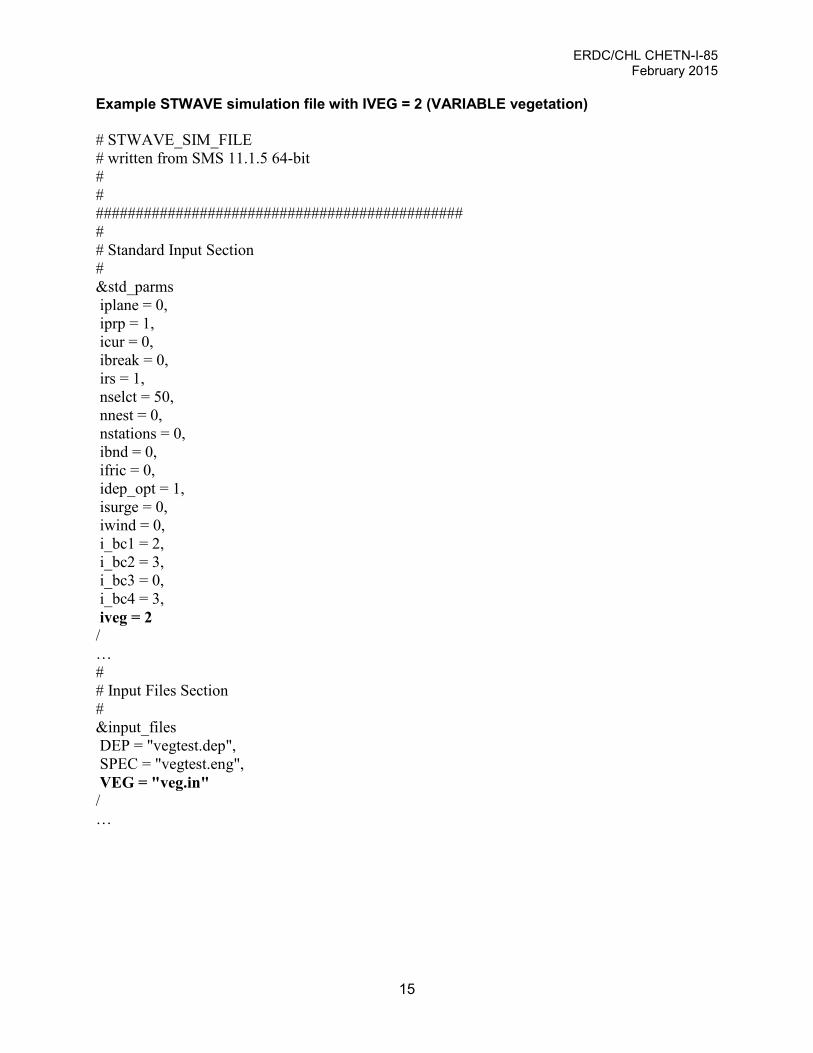
Example STWAVE simulation file with IVEG = 2 (VARIABLE vegetation) # STWAVE_SIM_FILE # written from SMS 11.1.5 64-bit # # ############################################## # # Standard Input Section # &std_parms iplane = 0, iprp = 1, icur = 0, ibreak = 0, irs = 1, nselct = 50, nnest = 0, nstations = 0, ibnd = 0, ifric = 0, idep_opt = 1, isurge = 0, iwind = 0, i_bc1 = 2, i_bc2 = 3, i_bc3 = 0, i_bc4 = 3, iveg = 2 / … # # Input Files Section # &input_files DEP = "vegtest.dep", SPEC = "vegtest.eng", VEG = "veg.in" / …


16

APPENDIX B

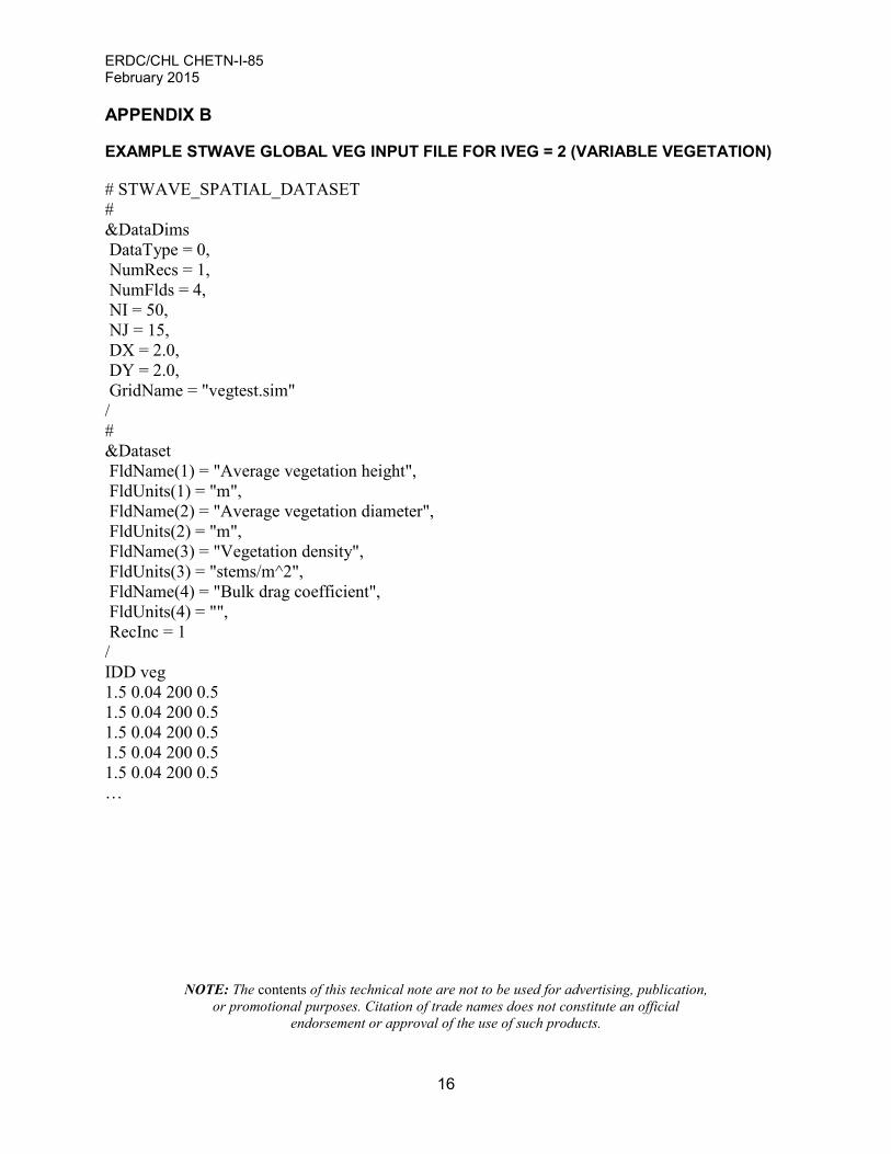
EXAMPLE STWAVE GLOBAL VEG INPUT FILE FOR IVEG = 2 (VARIABLE VEGETATION)

# STWAVE_SPATIAL_DATASET # &DataDims DataType = 0, NumRecs = 1, NumFlds = 4, NI = 50, NJ = 15, DX = 2.0, DY = 2.0, GridName = "vegtest.sim" / # &Dataset FldName(1) = "Average vegetation height", FldUnits(1) = "m", FldName(2) = "Average vegetation diameter", FldUnits(2) = "m", FldName(3) = "Vegetation density", FldUnits(3) = "stems/m^2", FldName(4) = "Bulk drag coefficient", FldUnits(4) = "", RecInc = 1 / IDD veg 1.5 0.04 200 0.5 1.5 0.04 200 0.5 1.5 0.04 200 0.5 1.5 0.04 200 0.5 1.5 0.04 200 0.5 …

NOTE: The contents of this technical note are not to be used for advertising, publication, or promotional purposes. Citation of trade names does not constitute an official

endorsement or approval of the use of such products.

Documents

Implementation of Wave Dissipation by Vegetation in STWAVE · Implementation of Wave Dissipation by Vegetation in STWAVE ... Implementation of Wave Dissipation by Vegetation in