Analysis of Measured and Predicted Acousticsfrom an XV-15 Flight Test

D. Douglas Boyd, Jr.Casey L. Burley

Aeroacoustics BranchNASA Langley Research Center

Hampton, VA.

Abstract

Flight acoustic and vehicle state data from an XV-15 acoustic flight test are examined. Flight predic-tions using TRAC are performed for a level flight(repeated) and four descent conditions (includinga BVI). The assumptions and procedures used forTRAC flight predictions as well as the variabilityin flight measurements, which are used for inputand comparison to predictions, are investigated indetail. Differences were found in the measured ve-hicle airspeed, altitude, glideslope, and vehicle ori-entation (yaw, pitch and roll angle) between eachof the repeat runs. These differences violate someof the prediction assumptions and significantly im-pacted the resulting acoustic predictions. Multi-ple acoustic pulses, with a variable time betweenthe pulses, were found in the measured acoustictime histories for the repeat runs. These differencescould be attributed in part to the variability in ve-hicle orientation. Acoustic predictions that usedthe measured vehicle orientation for the repeat runscaptured this multiple pulse variability. Thicknessnoise was found to be dominant on approach forall the cases, except the BVI condition. After theaircraft passed overhead, broadband noise and lowfrequency loading noise were dominant. The pre-dicted LowSPL time histories compared well withmeasurement on approach to the array for the non-BVI conditions and poorly for the BVI condition.

Presented at the American Helicopter Society 57th Forum,Washington, DC, May 9-11, 2001. Copyright c 2001 by theAmerican Helicopter Society, Inc. All rights reserved.

Accurate prediction of the lift share between the ro-tor and fuselage must be known in order to improvepredictions. At a minimum, measurements of therotor thrust and tip-path-plane angle are critical tofurther develop accurate flight acoustic predictioncapabilities.

Symbols

BPF blade passage frequencyBVI blade-vortex interactionBWI blade-wake interactiondB decibelHz Hertz [sec�1]i nacelle tilt angle [̊ ]kHz 1000 Hertz [sec�1]LowSPL SPL for � 5 BPF [dB]M flight Mach numberMidSPL SPL for > 5 BPF and � 40 BPF [dB]P1 measured acoustic pressure [Pa]P2 normalized acoustic pressure [Pa]OASPL overall sound pressure level [dB]r1 distance to microphone [ft]r2 normalizing distance [ft]SPL sound pressure level [dB]t time coordinate [sec]T1 measured period [sec]T2 de-Dopplerized period [sec]V aircraft velocity [kts]γ glide slope [̊ ]θe acoustic emission angle [̊ ]

https://ntrs.nasa.gov/search.jsp?R=20050042021 2020-04-02T06:25:59+00:00Z

2

Introduction

Tiltrotor aircraft, which take off and land verti-cally like a helicopter and fly like conventional air-planes during cruise, provide a potential alternativemeans of civilian transportation that could increaseairport capacity without consuming large tracts ofland. However, for tiltrotor aircraft to be a suc-cessful component of the civil aviation market, theymust be perceived by the public as an acceptablyquiet, safe, and economical mode of transportation.The noise impact of these aircraft, particularly dur-ing descent into airports, has been identified as abarrier issue for civil tiltrotor acceptance by the pub-lic. The Short Haul Civil Tiltrotor SH(CT) Programunder the Advanced Subsonic Transport (AST) ini-tiative was tasked to address the critical issues thatwould enable the acceptance of the civil tiltrotor air-craft [1]. Under the SH(CT) program a number offlight and wind tunnel tests have been conducted toinvestigate and demonstrate advanced technologiesrelated to civil tiltrotor aircraft. To date, flight testshave focused mainly on the examination of safe,low-noise terminal area operations and noise abate-ment procedures for approach operations [2, 3, 4, 5].Results from these test are usually presented as acomparison of several noise metrics for the vari-ous conditions flown. Wind tunnel tests have fo-cused primarily on determining the basic aerody-namic and aeroacoustic characteristics of differentproprotor designs [6, 7, 8, 9].

In addition to the experimental work, tiltrotoraeroacoustic prediction methodologies were, andcontinue to be, developed. One such predic-tion methodology developed under SH(CT) is theTiltRotor Aeroacoustic Code (TRAC) system [10,11, 12, 13, 14]. TRAC’s objective is to provideanalysis for evaluation and design of efficient, low-noise tiltrotors and to support the development ofsafe, low-noise flight profiles. To date, the primaryfocus in the TRAC system has been on methodol-ogy development based on isolated rotor wind tun-nel tests. Recently, however, high quality flightdata have become available and preliminary com-parisons between measured and predicted data havebeen made [15, 16]. Initial TRAC predictions foran XV-15 tiltrotor were presented by Prichard [15].In this paper, a more detailed examination of XV-15

flight data is made, and the relationship of that datato requirements of prediction efforts is outlined.

This paper is divided into three parts. The firstpart discusses the prediction methodology and as-sumptions typically used in TRAC. The second partpresents an analysis of the measured data for sev-eral flight conditions. Quantities examined includeaircraft state data, acoustic pressure time histories,and integrated noise metrics. The third part presentscomparisons of predicted and measured data fornominal and off-nominal conditions.

Prediction Methodology

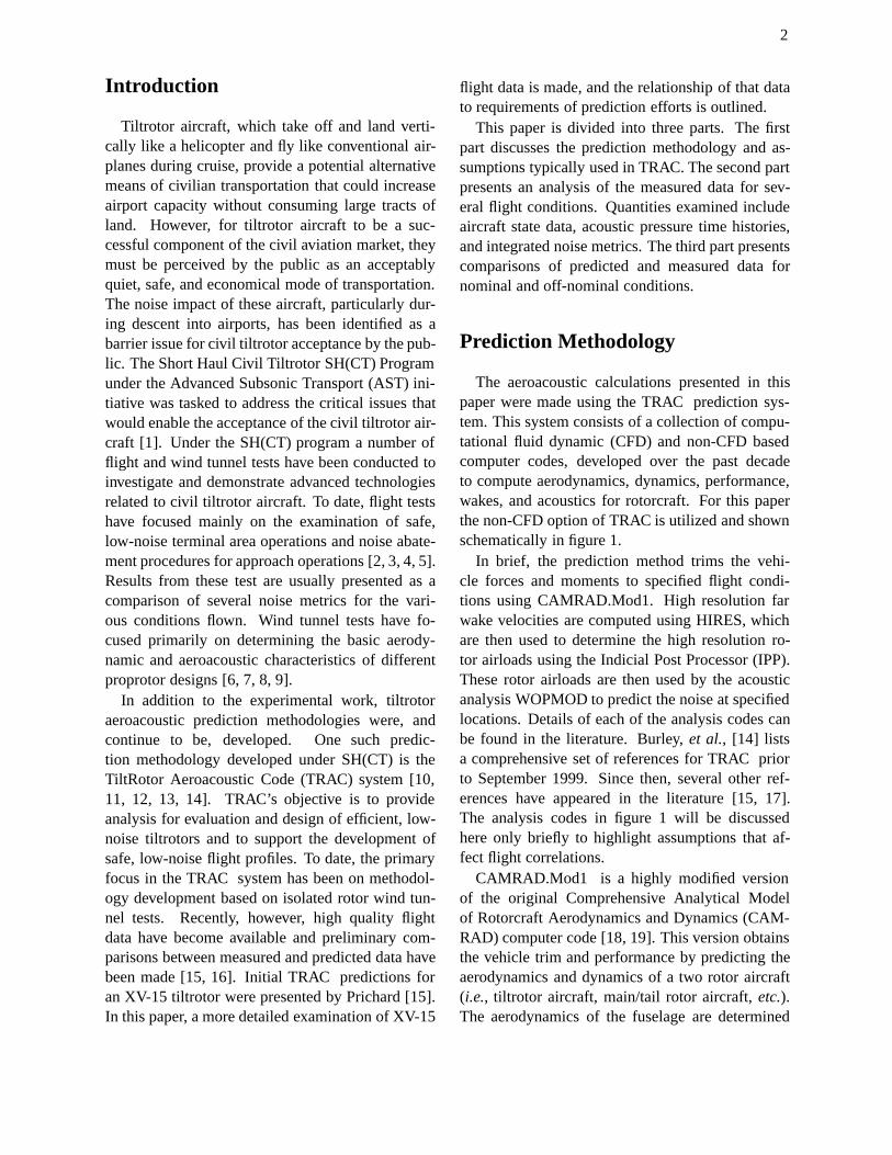
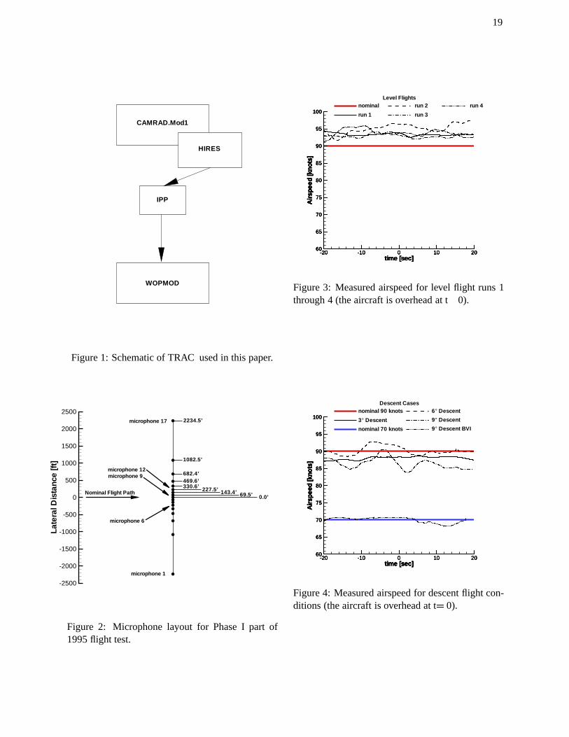
The aeroacoustic calculations presented in thispaper were made using the TRAC prediction sys-tem. This system consists of a collection of compu-tational fluid dynamic (CFD) and non-CFD basedcomputer codes, developed over the past decadeto compute aerodynamics, dynamics, performance,wakes, and acoustics for rotorcraft. For this paperthe non-CFD option of TRAC is utilized and shownschematically in figure 1.

In brief, the prediction method trims the vehi-cle forces and moments to specified flight condi-tions using CAMRAD.Mod1. High resolution farwake velocities are computed using HIRES, whichare then used to determine the high resolution ro-tor airloads using the Indicial Post Processor (IPP).These rotor airloads are then used by the acousticanalysis WOPMOD to predict the noise at specifiedlocations. Details of each of the analysis codes canbe found in the literature. Burley, et al., [14] listsa comprehensive set of references for TRAC priorto September 1999. Since then, several other ref-erences have appeared in the literature [15, 17].The analysis codes in figure 1 will be discussedhere only briefly to highlight assumptions that af-fect flight correlations.

CAMRAD.Mod1 is a highly modified versionof the original Comprehensive Analytical Modelof Rotorcraft Aerodynamics and Dynamics (CAM-RAD) computer code [18, 19]. This version obtainsthe vehicle trim and performance by predicting theaerodynamics and dynamics of a two rotor aircraft(i.e., tiltrotor aircraft, main/tail rotor aircraft, etc.).The aerodynamics of the fuselage are determined

3

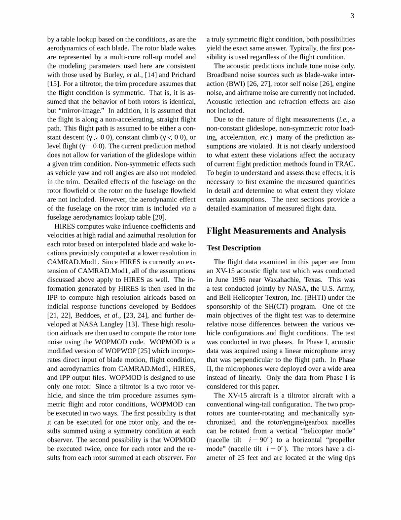
by a table lookup based on the conditions, as are theaerodynamics of each blade. The rotor blade wakesare represented by a multi-core roll-up model andthe modeling parameters used here are consistentwith those used by Burley, et al., [14] and Prichard[15]. For a tiltrotor, the trim procedure assumes thatthe flight condition is symmetric. That is, it is as-sumed that the behavior of both rotors is identical,but “mirror-image.” In addition, it is assumed thatthe flight is along a non-accelerating, straight flightpath. This flight path is assumed to be either a con-stant descent (γ> 0:0), constant climb (γ< 0:0), orlevel flight (γ= 0:0). The current prediction methoddoes not allow for variation of the glideslope withina given trim condition. Non-symmetric effects suchas vehicle yaw and roll angles are also not modeledin the trim. Detailed effects of the fuselage on therotor flowfield or the rotor on the fuselage flowfieldare not included. However, the aerodynamic effectof the fuselage on the rotor trim is included via afuselage aerodynamics lookup table [20].

HIRES computes wake influence coefficients andvelocities at high radial and azimuthal resolution foreach rotor based on interpolated blade and wake lo-cations previously computed at a lower resolution inCAMRAD.Mod1. Since HIRES is currently an ex-tension of CAMRAD.Mod1, all of the assumptionsdiscussed above apply to HIRES as well. The in-formation generated by HIRES is then used in theIPP to compute high resolution airloads based onindicial response functions developed by Beddoes[21, 22], Beddoes, et al., [23, 24], and further de-veloped at NASA Langley [13]. These high resolu-tion airloads are then used to compute the rotor tonenoise using the WOPMOD code. WOPMOD is amodified version of WOPWOP [25] which incorpo-rates direct input of blade motion, flight condition,and aerodynamics from CAMRAD.Mod1, HIRES,and IPP output files. WOPMOD is designed to useonly one rotor. Since a tiltrotor is a two rotor ve-hicle, and since the trim procedure assumes sym-metric flight and rotor conditions, WOPMOD canbe executed in two ways. The first possibility is thatit can be executed for one rotor only, and the re-sults summed using a symmetry condition at eachobserver. The second possibility is that WOPMODbe executed twice, once for each rotor and the re-sults from each rotor summed at each observer. For

a truly symmetric flight condition, both possibilitiesyield the exact same answer. Typically, the first pos-sibility is used regardless of the flight condition.

The acoustic predictions include tone noise only.Broadband noise sources such as blade-wake inter-action (BWI) [26, 27], rotor self noise [26], enginenoise, and airframe noise are currently not included.Acoustic reflection and refraction effects are alsonot included.

Due to the nature of flight measurements (i.e., anon-constant glideslope, non-symmetric rotor load-ing, acceleration, etc.) many of the prediction as-sumptions are violated. It is not clearly understoodto what extent these violations affect the accuracyof current flight prediction methods found in TRAC.To begin to understand and assess these effects, it isnecessary to first examine the measured quantitiesin detail and determine to what extent they violatecertain assumptions. The next sections provide adetailed examination of measured flight data.

Flight Measurements and Analysis

Test Description

The flight data examined in this paper are froman XV-15 acoustic flight test which was conductedin June 1995 near Waxahachie, Texas. This wasa test conducted jointly by NASA, the U.S. Army,and Bell Helicopter Textron, Inc. (BHTI) under thesponsorship of the SH(CT) program. One of themain objectives of the flight test was to determinerelative noise differences between the various ve-hicle configurations and flight conditions. The testwas conducted in two phases. In Phase I, acousticdata was acquired using a linear microphone arraythat was perpendicular to the flight path. In PhaseII, the microphones were deployed over a wide areainstead of linearly. Only the data from Phase I isconsidered for this paper.

The XV-15 aircraft is a tiltrotor aircraft with aconventional wing-tail configuration. The two prop-rotors are counter-rotating and mechanically syn-chronized, and the rotor/engine/gearbox nacellescan be rotated from a vertical “helicopter mode”(nacelle tilt i = 90˚ ) to a horizontal “propellermode” (nacelle tilt i = 0˚ ). The rotors have a di-ameter of 25 feet and are located at the wing tips

4

which are approximately 16 feet from the aircraftcenterline. Specific design details of the aircraft, in-cluding the flight envelope, are provided in refer-ence [28].

Flight Measurements

For each flight run, acoustic data as well as aircraftstate and aircraft position (tracking) data were ob-tained. The test matrix included a range of nacelletilts, airspeeds, and glideslopes (descent angles) [5].

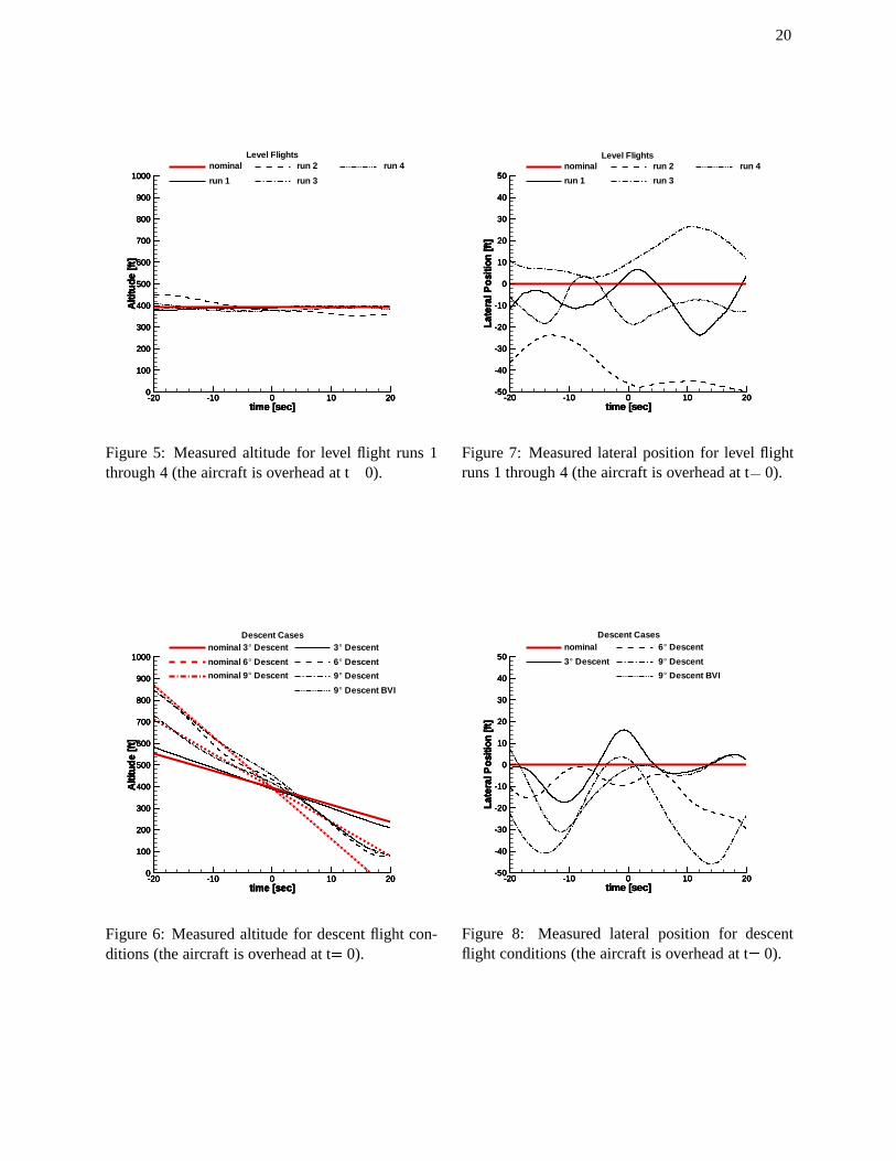
The acoustic data were obtained during the testby flying the aircraft over a linear array of 17 groundboard, flush mounted microphones deployed per-pendicular to the flight path, as shown schematicallyin Figure 2. The microphone array is oriented per-pendicular to the nominal flight path. The unequalmicrophone spacing was designed such that, whenthe aircraft is 394 feet directly over the array, themicrophones are spaced at a 10˚ angular resolutionto both sidelines [4]. For reference, microphone #9is the centerline microphone, that is, it is directly inline with the nominal flight path. In this paper, datafrom microphones #9 (located on the centerline), #6(located 227.5 feet to starboard of the centerline),and #12 (located 227.5 feet to port of the centerline)are examined in detail.

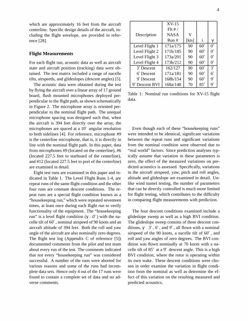
Eight test runs are examined in this paper and in-dicated in Table 1. The Level Flight Runs 1-4, arerepeat runs of the same flight condition and the otherfour runs are constant descent conditions. The re-peat runs are a special flight condition known as a“housekeeping run,” which were repeated seventeentimes, at least once during each flight run to verifyfunctionality of the equipment. The “housekeepingrun” is a level flight condition (γ=0˚ ) with the na-celle tilt of 60˚ , nominal airspeed of 90 knots and anaircraft altitude of 394 feet. Both the roll and yawangle of the aircraft are also nominally zero degrees.The flight test log (Appendix C of reference [5])documented comments from the pilot and test teamabout every run of the test. The comments indicatedthat not every “housekeeping run” was consideredsuccessful. A number of the runs were aborted forvarious reasons and some of the runs had incom-plete data sets. Hence only 4 out of the 17 runs werefound to contain a complete set of data and no ad-verse comments.

XV-15Flt # /

Description NASA VRun # [kts] i γ

Level Flight 1 171a/175 90 60˚ 0˚Level Flight 2 171b/185 90 60˚ 0˚Level Flight 3 173a/201 90 60˚ 0˚Level Flight 4 173b/212 90 60˚ 0˚

3˚ Descent 162/127 90 60˚ 3˚6˚ Descent 171a/181 90 60˚ 6˚9˚ Descent 168b/154 90 60˚ 9˚

9˚ Descent BVI 168a/148 70 85˚ 9˚

Table 1: Nominal run conditions for XV-15 flightdata.

Even though each of these “housekeeping runs”were intended to be identical, significant variationsbetween the repeat runs and significant variationsfrom the nominal condition were observed due to“real world” factors. Since prediction analyses typ-ically assume that variation in these parameters iszero, the effect of the measured variations on pre-dicted acoustics is assessed. Specifically, variationsin the aircraft airspeed, yaw, pitch and roll angles,altitude and glideslope are examined in detail. Un-like wind tunnel testing, the number of parametersthat can be directly controlled is much more limitedfor flight testing, which contributes to the difficultyin comparing flight measurements with prediction.

The four descent conditions examined include aglideslope sweep as well as a high BVI condition.The glideslope sweep consists of three descent con-ditions, γ=3˚ , 6˚ , and 9˚ , all flown with a nominalairspeed of the 90 knots, a nacelle tilt of 60˚ , androll and yaw angles of zero degrees. The BVI con-dition was flown nominally at 70 knots with a na-celle tilt of 85˚ at a 9˚ descent angle. This is a highBVI condition, where the rotor is operating withinits own wake. These descent conditions were cho-sen in order examine the variation in flight condi-tion from the nominal as well as determine the ef-fect of this variation on the resulting measured andpredicted acoustics.

5

Aircraft State Data

An onboard recording system monitored a num-ber of basic aircraft flight parameters and operatingconditions. These parameters were recorded andstored at various sample rates, but were all timesynchronized using GPS time code. For this pa-per, the raw onboard data was smoothed using a 3second moving average. Since the parameters wererecorded at various sample rates, after smoothing,they were re-sampled at a rate of once per revolu-tion. In addition, the aircraft position was monitoredusing a laser tracking system accurate to within�1 foot in range and 0:1 mrad in azimuth and el-evation [4].

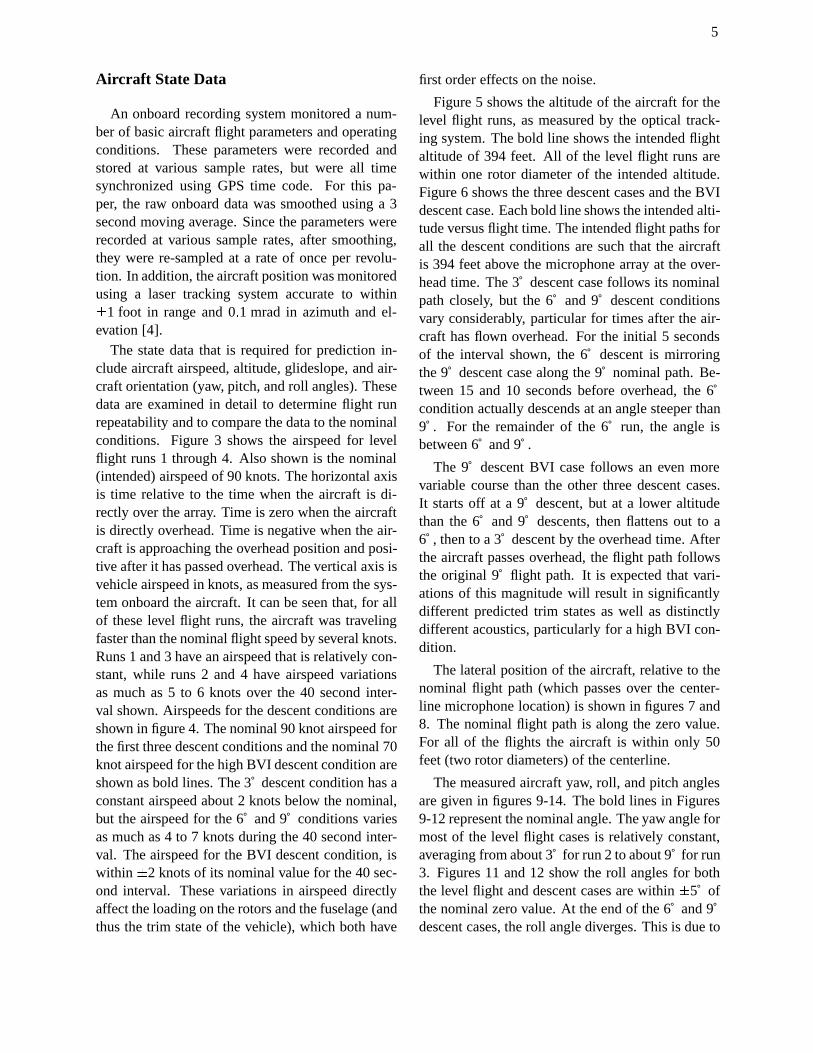
The state data that is required for prediction in-clude aircraft airspeed, altitude, glideslope, and air-craft orientation (yaw, pitch, and roll angles). Thesedata are examined in detail to determine flight runrepeatability and to compare the data to the nominalconditions. Figure 3 shows the airspeed for levelflight runs 1 through 4. Also shown is the nominal(intended) airspeed of 90 knots. The horizontal axisis time relative to the time when the aircraft is di-rectly over the array. Time is zero when the aircraftis directly overhead. Time is negative when the air-craft is approaching the overhead position and posi-tive after it has passed overhead. The vertical axis isvehicle airspeed in knots, as measured from the sys-tem onboard the aircraft. It can be seen that, for allof these level flight runs, the aircraft was travelingfaster than the nominal flight speed by several knots.Runs 1 and 3 have an airspeed that is relatively con-stant, while runs 2 and 4 have airspeed variationsas much as 5 to 6 knots over the 40 second inter-val shown. Airspeeds for the descent conditions areshown in figure 4. The nominal 90 knot airspeed forthe first three descent conditions and the nominal 70knot airspeed for the high BVI descent condition areshown as bold lines. The 3˚ descent condition has aconstant airspeed about 2 knots below the nominal,but the airspeed for the 6˚ and 9˚ conditions variesas much as 4 to 7 knots during the 40 second inter-val. The airspeed for the BVI descent condition, iswithin �2 knots of its nominal value for the 40 sec-ond interval. These variations in airspeed directlyaffect the loading on the rotors and the fuselage (andthus the trim state of the vehicle), which both have

first order effects on the noise.

Figure 5 shows the altitude of the aircraft for thelevel flight runs, as measured by the optical track-ing system. The bold line shows the intended flightaltitude of 394 feet. All of the level flight runs arewithin one rotor diameter of the intended altitude.Figure 6 shows the three descent cases and the BVIdescent case. Each bold line shows the intended alti-tude versus flight time. The intended flight paths forall the descent conditions are such that the aircraftis 394 feet above the microphone array at the over-head time. The 3˚ descent case follows its nominalpath closely, but the 6˚ and 9˚ descent conditionsvary considerably, particular for times after the air-craft has flown overhead. For the initial 5 secondsof the interval shown, the 6˚ descent is mirroringthe 9˚ descent case along the 9˚ nominal path. Be-tween 15 and 10 seconds before overhead, the 6˚condition actually descends at an angle steeper than9˚ . For the remainder of the 6˚ run, the angle isbetween 6˚ and 9˚ .

The 9˚ descent BVI case follows an even morevariable course than the other three descent cases.It starts off at a 9˚ descent, but at a lower altitudethan the 6˚ and 9˚ descents, then flattens out to a6˚ , then to a 3˚ descent by the overhead time. Afterthe aircraft passes overhead, the flight path followsthe original 9˚ flight path. It is expected that vari-ations of this magnitude will result in significantlydifferent predicted trim states as well as distinctlydifferent acoustics, particularly for a high BVI con-dition.

The lateral position of the aircraft, relative to thenominal flight path (which passes over the center-line microphone location) is shown in figures 7 and8. The nominal flight path is along the zero value.For all of the flights the aircraft is within only 50feet (two rotor diameters) of the centerline.

The measured aircraft yaw, roll, and pitch anglesare given in figures 9-14. The bold lines in Figures9-12 represent the nominal angle. The yaw angle formost of the level flight cases is relatively constant,averaging from about 3˚ for run 2 to about 9˚ for run3. Figures 11 and 12 show the roll angles for boththe level flight and descent cases are within �5˚ ofthe nominal zero value. At the end of the 6˚ and 9˚descent cases, the roll angle diverges. This is due to

6

the pilot “peeling off” and departing the area at theend of the run.

The fuselage pitch angle relative to the horizon isshown in figures 13 and 14. There is not a nominalpitch angle, since the fuselage pitch is a functionof the aircraft trim condition. For the level flightconditions, the pitch varies between 2˚ and 5˚ . Thesame order of variation is seen for the descent cases,however the average pitch between each case variessubstantially more than for the level flight cases.For the 9˚ descent BVI condition, the pitch is rel-atively constant at approximately a 4.5˚ nose-downattitude.

To fly a prescribed flight condition, the pilot mustcontinuously monitor the flight state and make ad-justments to maintain that condition. Hence thevariations noted in airspeed, altitude, and vehicleorientation are due to the pilot maintaining a givenflight condition and flight path. These variationswill be shown to significantly affect the characterand amplitude of resulting acoustic time histories,as well as the overall directivity of the noise.

Flight Acoustic Data

The primary focus of the 1995 XV-15 flight testwas to compare acoustic footprints for various ter-minal area operations, such as takeoff and landing[4]. These comparisons were based on a set of A-weighted, integrated noise metrics such as the Over-all Sound Pressure Level (OASPL). Examination ofthese integrated metrics is appropriate for compar-isons of various terminal area operations. However,for assessment of capabilities of prediction tools andfor understanding the underlying noise mechanismsinvolved, examination of acoustic time histories isessential. This can be seen specifically in the acous-tic aspects of prediction work by realizing that anynumber of acoustic pressure time histories, or wave-forms, are capable of generating the exact sameOASPL. Therefore, it is more important to exam-ine the fundamental quantities, such as the acous-tic pressure time histories, rather than just the in-tegrated quantities when assessing a prediction toolor when trying to understand the underlying physicsof the noise mechanisms involved. Indeed, if thesefundamental quantities are predicted correctly, thepredicted integrated metrics will be correct as well.

So, the primary data of interest when comparingprediction to acoustic flight measurements, is theacoustic pressure time history. All other noise met-rics can be derived from the acoustic pressure timehistories, if desired. Hence, the pressure time histo-ries will be discussed and presented in detail.

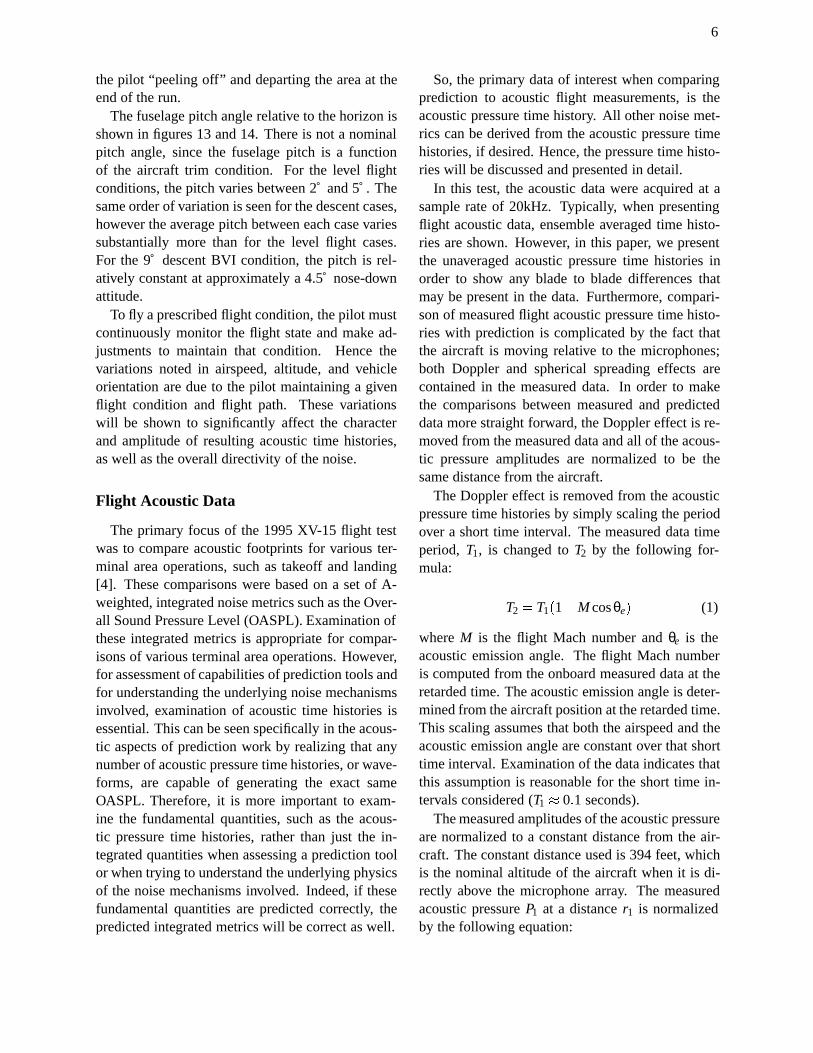
In this test, the acoustic data were acquired at asample rate of 20kHz. Typically, when presentingflight acoustic data, ensemble averaged time histo-ries are shown. However, in this paper, we presentthe unaveraged acoustic pressure time histories inorder to show any blade to blade differences thatmay be present in the data. Furthermore, compari-son of measured flight acoustic pressure time histo-ries with prediction is complicated by the fact thatthe aircraft is moving relative to the microphones;both Doppler and spherical spreading effects arecontained in the measured data. In order to makethe comparisons between measured and predicteddata more straight forward, the Doppler effect is re-moved from the measured data and all of the acous-tic pressure amplitudes are normalized to be thesame distance from the aircraft.

The Doppler effect is removed from the acousticpressure time histories by simply scaling the periodover a short time interval. The measured data timeperiod, T1, is changed to T2 by the following for-mula:

T2 = T1(1�M cosθe) (1)

where M is the flight Mach number and θe is theacoustic emission angle. The flight Mach numberis computed from the onboard measured data at theretarded time. The acoustic emission angle is deter-mined from the aircraft position at the retarded time.This scaling assumes that both the airspeed and theacoustic emission angle are constant over that shorttime interval. Examination of the data indicates thatthis assumption is reasonable for the short time in-tervals considered (T1 � 0:1 seconds).

The measured amplitudes of the acoustic pressureare normalized to a constant distance from the air-craft. The constant distance used is 394 feet, whichis the nominal altitude of the aircraft when it is di-rectly above the microphone array. The measuredacoustic pressure P1 at a distance r1 is normalizedby the following equation:

7

P2 = P1

�r1

r2

�: (2)

where r2 = 394 feet. The normalized values are pre-sented in the figures.

In addition to examination of individual acousticpressure time histories, two integrated spectral met-rics (“LowSPL” and “MidSPL”) are also examinedand presented in the form of acoustic “footprints.”LowSPL represents the low frequency acoustic con-tent and MidSPL represents the higher frequencyacoustic content for which BVI noise is dominant.The computation of these two metrics is as fol-lows. For a given flight time and microphone, threecontiguous acoustic pressure time history segments,consisting of 4096 points each, are extracted fromthe raw data. The effect of spherical spreading isremoved by applying equation (2) to the acousticpressures. This set of three contiguous time histo-ries, consisting of 12288 points in all, is centered onthe current time at the current microphone as shownin figure 15. Based on the number of points andthe sample rate of 20 kHz, each window occupies a0:2048 second time interval, which corresponds toapproximately two rotor revolutions of data. Thesethree time segments are labeled 1, 2, and 3 in fig-ure 15. Using the data in the three time historysegments, two additional overlapping time historysegments, labeled 4 and 5 are constructed. To re-duce the effects of a finite length segment on the re-sults, a Hamming window [29] function is appliedto each of the five time history segments. Then, aFast Fourier Transform (FFT) is taken to determinethe spectral content of each segment. The spectrafrom these overlapping segments are then ensembleaveraged to reduce statistical variability [30] of thespectrum. The Doppler effect is removed from thespectra by applying equation (1).

Once the spectra are computed for all flight timesand all microphones, the LowSPL and MidSPLcomponents are computed. The LowSPL metric iscomputed by summing all of the spectral contribu-tions up to the 5th blade passage frequency (BPF).The MidSPL metric is computed by summing all ofthe spectral contributions between the 5th BPF andthe 40th BPF.

Acoustic Time Histories: Housekeeping Runs

The variability of the acoustic pressures for eachof the housekeeping runs is considered by examin-ing the unaveraged acoustic pressure time historiesof length 0.1 seconds. The 0:1 second time inter-val was chosen because it is almost exactly equalto one rotor revolution. (Actually, at the nominal589 RPM, one rotor revolution is equal to a periodof 0:1018 seconds.) Figures 16-18 show the un-averaged time histories for all four level flight runs.Both the Doppler effect and the spherical spreadingeffect have been removed.

Each figure, contains time histories that are sam-pled 5 seconds apart, ranging from 15 seconds priorto the aircraft passing over the array (labeled “15sec prior”) to 5 seconds after the aircraft has passedover the array (labeled “5 sec after”). When the air-craft is directly over the array time history is labeled“overhead.” Here, the time relative to the overheadtime refers to the flight time as measured by the op-tical tracking system, not the retarded time. Notethat in all of the plots, the horizontal axes have thesame time scale, which is the 0:1 second intervalcentered on the time relative to overhead. However,the scale on the vertical axis changes. Before theoverhead time, the vertical scale ranges from -50 to20 Pascals. At overhead and later, the vertical scaleis expanded to range from -10 to 10 Pascals in orderto better show the signature details.

The four housekeeping runs have similarities aswell as notable differences. For all times prior tothe aircraft passing the array, nearly all the acousticsignals are dominated by impulsive events that in-crease in amplitude as the aircraft approaches the ar-ray. Using a simple analysis based on the airspeed,altitude of the aircraft and the rotor shaft tilt, it canbe shown that the microphones are in the plane ofthe rotor when the aircraft is 5 seconds prior to over-head. Thickness noise is generally dominant in therotor plane and typically appears as strong negativeimpulses in the acoustic time history. Most of themeasured acoustic pressure time histories at 5 sec-onds prior contain strong negative pulse(s) whichare attributed to thickness noise. This is also foundto be supported by examining the components of thepredicted noise at these locations. It is not expected

8

that there would be strong BVI noise measured atthis location for this level flight condition.

Even though the four housekeeping runs were in-tended to be identical, some of the time histories arequite different. For level flight run 3, (figure 16) forthe 15, 10, and 5 seconds prior to overhead there is alarge “double peak” in the signal. The double peaksare much less evident in the data from runs 1, 2 and4. Assuming that each peak comes from a differentrotor, then the time between the two pulses (multi-plied by the speed of sound) is a measure of the dif-ference in distance that the sound traveled from thetwo sources to the microphone. Since the aircraftis symmetric, and the microphone is on the nominalflight path centerline, then the cause of the extra dis-tance traveled can be associated with some combi-nation of the aircraft being laterally displaced fromthe nominal centerline, the aircraft being at a non-zero roll angle, or the aircraft being at a non-zeroyaw angle. Based on the measured time between thepulses for run 3 at 5 seconds prior to overhead, thedistance between the two sources is approximately5 feet. This difference is well within the variabilityof the vehicle location during the flight runs.

To the authors’ knowledge, the first documenta-tion of these double acoustic peaks for the XV-15was in 1987 by Brieger, et al., [31]. There, forslightly different flight conditions and with the ro-tors configured out of phase by 4˚ of azimuth, theyshowed similar results to those presented here. Theyalso suggested that the double peak is not relatedto the 4˚ of rotor phasing. That conclusion is sup-ported here since there is no rotor phasing in thistest, yet similar double peaks are still found.

When the aircraft is directly over the array, thesignal is dominated by low frequency blade load-ing noise and broadband noise, which is seen ashigh frequency signal superimposed on the lowerfrequency loading noise. The negative pulse seenat earlier times is essentially nonexistent. Actuallysince the rotors have a nacelle tilt of 60˚ the mi-crophones are not directly below (and perpendicularto) the rotor plane until the approximately one sec-ond after the aircraft is overhead. The difference be-tween the acoustic signal at that time and overheadis negligible, but between that time and 5 secondsafter overhead the low frequency loading noise de-creases considerably. Once the aircraft is 5 seconds

past overhead, the signal is dominated by broadbandnoise. The character of the broadband signal sug-gests that it is associated with rotor broadband noiserather than engine or airframe noise. For times laterthan 5 seconds after overhead, the broadband char-acter of the signal is found to decay rapidly. Also,the impulsive character of the signal in this region isabsent and has been replaced by a much smootherblade passage event with a frequency indicative ofblade loading noise. Also of note is that, for anygiven run, blade to blade differences are very small.

These differences in the “identical” level flightconditions have implications for prediction work.It is important to be aware of the kinds and levelsof differences in the measured data. For example,a common technique for prediction of a nominallylevel flight condition is to assume that there is aplane of symmetry. This assumption of symmetryleads to the conclusion that it is not possible to havea double peak even at the centerline microphone (asseen in figure 16, run 3). However, the measureddata show that relatively small perturbations to thatlevel flight condition can create large changes in thecharacter of the measured acoustics (e.g., having nodouble peak event vs having a double peak event).

Figures 17 and 18 are the same as the previousfigure, except the data are from the symmetricallyplaced sideline microphones 6 and 12. The datatrends are similar to those observed for the center-line microphone. However, as expected, the exis-tence of double peaks is much more prevalent. Thisis in part attributed to the distance differences be-tween each rotor and the microphone, due to the ro-tor orientation and as well as its location.

Comparison of the signals from microphones 6and 12 (figures 17 and 18) show that they are quitesimilar to each other. The primary difference ap-pears to be that the acoustic pressure double peaksare separated by slightly different times. By assum-ing that the double peak is composed of one peakfrom each rotor, which is supported by the similar-ity of the two pulses in the double peak event, it canbe seen that the two rotors are generating similaracoustic signatures which arrive at the microphoneat slightly different times. Furthermore, since thetime between the two peaks is different between theport and starboard microphones, this indicates thatthe aircraft is not symmetrically oriented and is dis-

9

placed from the nominal flight path and orientation.The aircraft tracking data supports this (see figures7, 9, and 11).

For prediction work, the assumption of symme-try leads to the conclusion that that the two sidelinemicrophones discussed above should have the ex-act same measured acoustics. From this analysis,it is clear that for flight data this situation is neverexactly the case, even for explicitly defined repeatflight conditions.

Acoustic Time Histories: Descent Cases

Figures 19-21 show acoustic pressure time his-tories for the three different descent angles and theone BVI condition. On examination of the first threedescent cases, one of the most noticeable featuresis that, for times at and after the overhead time,the character of the acoustic pressure signals is thesame for the different descent conditions. In addi-tion, the character of these signals is essentially asthat found in all of the level flight runs shown previ-ously. As noted then, the signals appear to be thick-ness noise dominated. For times before the over-head time, the dominant feature in the these threedescent cases is the double peak event. Some ofthese double peak events also have smaller pulsessuperimposed on them. For example, for the 6˚ de-scent case in figure 19, in the “15 sec prior” and the“10 sec prior” plots, the pulses are not smooth, butrather have other pulses included. It is speculatedthat these are small BVI events.

Examination of the 9˚ descent BVI condition, asmeasured from the centerline microphone, (figure19) reveals a smooth pulse preceded by a substan-tial BVI event. These features are similar for all ofthe times prior to overhead. As expected the sig-nals from the sideline microphones (figures 20 and21) show double the BVI activity. For some of thetimes, the pulse separation times at microphone 6and microphone 12 are substantially different. Forexample, in the “5 sec prior” plot for the 6˚ de-scent angle in figure 20, the pulses are almost evenlyspaced. However, the corresponding plot for micro-phone 12 in figure 21, the pulses are very close to-gether. For this condition there is considerable vari-ation in the aircraft yaw, roll and pitch angles (see,figures 10, 12 and 14). The differences in distance

from each rotor to microphones 6 and 12 are suchas to warrant the difference in pulse separation. Aswith the centerline microphone data shown earlier,except for the actual BVI components of the signal,the remainder of the acoustic pressure time historieslook similar to the level flight conditions.

Integrated SPL

The integrated SPL metrics, LowSPL and Mid-SPL, are presented as time histories from the 3 mi-crophone locations (6, 9 and 12) and as directivitymaps.

LowSPL Time Histories

Figure 22 shows time histories of the LowSPLfor the centerline and sideline microphones for thefour level flights. In these plots, the horizontal axisis the time relative to the overhead time. This isthe same axis scale used in figures 3 through 14.The vertical axis is the LowSPL in dB and covers70 to 120 dB. The figures here come from integratedspectra plotted at each one second interval in the 40second interval on the horizontal axis.

In figure 22 for microphone 9, it can be seen thatthe LowSPL peaks about 5 seconds before the air-craft reaches the microphone array. As noted ear-lier, at this time the microphone array is in the planeof the rotor and the signal is dominated by thick-ness noise. There are relatively large variations inthe LowSPL for microphone 9 before the aircraftreaches the array. This variation was also noted forthe acoustic pressure time history, where a large sin-gle acoustic pulse was seen for run 1 and a smallerdouble peak was seen for run 3. After the aircraftpasses over the array (positive times on the horizon-tal axis), the LowSPL decreases rapidly. Since thesignal is then dominated by broadband noise (seefigures 16-18). Overall, all the LowSPL time his-tories from all three microphones are similar. Eventhough the details of the time histories are compa-rably different in character and amplitude (one peakvs double peaks).

The LowSPL time histories for the descent con-ditions are shown in figure 23. The first three de-scent cases look very similar in character to the levelflight cases. That is, the levels increase as the vehi-

10

cle approaches the array (time = 0), the levels peakaround 5 seconds before the vehicle is overhead, andthen the levels decrease rapidly after the overheadtime. All three descent cases fall within about a 5dB “band.” The BVI case, on the other hand, tendsto start off at a higher level and remain at that leveluntil passing over the array. Otherwise, it should benoted that these LowSPL values for the BVI case arenearly indistinguishable from the first three descentconditions.

LowSPL Contours

LowSPL directivity is presented in figure 24. Inall of these contour plots, the aircraft is located atthe origin and is pointing with its nose to the right.The horizontal axis shows the fore/aft angle. Thepositive angles are in front of the aircraft, zero de-grees points vertically downward, and the negativeangles are aft of the vehicle. The vertical axis isthe lateral angle. Positive angles are to starboardof the aircraft, zero degrees points vertically down-ward, and negative angles are to port. The actual di-rectivity angles are as determined from the aircrafttracking data.

Examination of figure 24 reveals that the max-imum noise is directed forward and down at ap-proximately the nacelle tilt angle. This is the thick-ness noise effect that has been shown previously inthe LowSPL time histories and shown in detail inthe acoustic pressure time histories. Aft of the air-craft on either side of the centerline are low noisezones. Though there are some minor differences,these overall characteristics prevail for all of thelevel flight runs.

Figure 25 shows similar contour plots for the de-scent cases. Note that the irregular boundary shapeof the figures is due to the usage of the actual di-rectivity angles computed from the aircraft track-ing data. The descent conditions, have the sameoverall contour map characteristic that was seen forthe level flight runs, with the exception of the BVIcondition. For the first three descent conditions,the maximum LowSPL occurs approximately in theplane of the rotor and minimum LowSPL occurs aftand to either side of the vehicle, as was the case forthe level flight conditions. The 9˚ BVI descent case,with the nacelle tilt at 85˚ and a fuselage nose down

pitch of approximately 4.5˚ , has a slightly differentdirectivity pattern. The maximum LowSPL is di-rected such that it is nearly in the plane of the rotor.

Similarities in all of these figures are seen despitethe differences seen in the acoustic pressure timehistories (i.e., the single pulses vs the double pulsesetc.). This is due to the fact that integration tendsto smooth out any differences. For prediction work,this has the implication that integrated noise met-ric are not necessarily the best mechanism availableto examine or assess the capabilities of a predictionmethod to properly model specific noise sources.

MidSPL Time Histories

MidSPL time histories are shown in figures 26and 27. (Note that the vertical axis range is nowfrom 40 to 100 dB.) It can be seen here that there isa large variation in the levels between the four levelflight runs, except in the 4 second interval aroundthe overhead time. The explanation for this can befound in the acoustic pressure time histories nearthe overhead time. Those show that broadband ro-tor noise with similar characteristics across the setof runs dominates the acoustics in the MidSPL fre-quency range near the overhead time. Even so, theMidSPL component shown here is almost insignifi-cant compared to the LowSPL values. For example,for the centerline microphone, the MidSPL peak isapproximately 30 dB below the LowSPL peak. Un-like the LowSPL, which was not symmetric aboutthe overhead position, the MidSPL plots are seen tobe symmetric about this point for all three micro-phones.

Figure 27 shows the MidSPL time histories forthe descent cases. The 3˚ and 9˚ descent conditionsshow similar characteristics to the level flight cases,but have an even larger variation in levels. The 6˚descent case is similar to the 3˚ and 9˚ descent forthe approach, but the MidSPL decreases far morerapidly than the other two cases. As for the BVIcase, as before, after the array has been passed, itbehaves like the 3˚ and 9˚ cases. However, on ap-proach, there is much more MidSPL content, due toBVI, which was clearly noted in the acoustic timehistories in figures 19-21.

11

MidSPL Contours

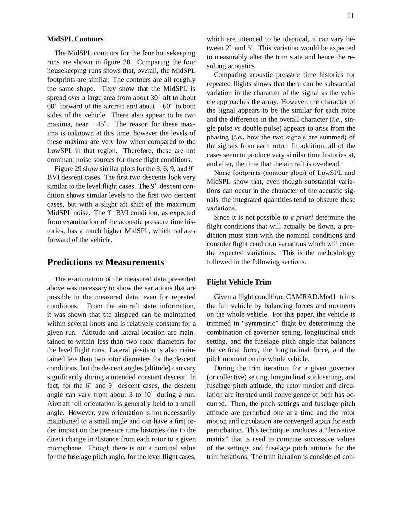
The MidSPL contours for the four housekeepingruns are shown in figure 28. Comparing the fourhousekeeping runs shows that, overall, the MidSPLfootprints are similar. The contours are all roughlythe same shape. They show that the MidSPL isspread over a large area from about 30˚ aft to about60˚ forward of the aircraft and about �60˚ to bothsides of the vehicle. There also appear to be twomaxima, near �45˚ . The reason for these max-ima is unknown at this time, however the levels ofthese maxima are very low when compared to theLowSPL in that region. Therefore, these are notdominant noise sources for these flight conditions.

Figure 29 show similar plots for the 3, 6, 9, and 9˚BVI descent cases. The first two descents look verysimilar to the level flight cases. The 9˚ descent con-dition shows similar levels to the first two descentcases, but with a slight aft shift of the maximumMidSPL noise. The 9˚ BVI condition, as expectedfrom examination of the acoustic pressure time his-tories, has a much higher MidSPL, which radiatesforward of the vehicle.

Predictions vs Measurements

The examination of the measured data presentedabove was necessary to show the variations that arepossible in the measured data, even for repeatedconditions. From the aircraft state information,it was shown that the airspeed can be maintainedwithin several knots and is relatively constant for agiven run. Altitude and lateral location are main-tained to within less than two rotor diameters forthe level flight runs. Lateral position is also main-tained less than two rotor diameters for the descentconditions, but the descent angles (altitude) can varysignificantly during a intended constant descent. Infact, for the 6˚ and 9˚ descent cases, the descentangle can vary from about 3 to 10˚ during a run.Aircraft roll orientation is generally held to a smallangle. However, yaw orientation is not necessarilymaintained to a small angle and can have a first or-der impact on the pressure time histories due to thedirect change in distance from each rotor to a givenmicrophone. Though there is not a nominal valuefor the fuselage pitch angle, for the level flight cases,

which are intended to be identical, it can vary be-tween 2˚ and 5˚ . This variation would be expectedto measurably alter the trim state and hence the re-sulting acoustics.

Comparing acoustic pressure time histories forrepeated flights shows that there can be substantialvariation in the character of the signal as the vehi-cle approaches the array. However, the character ofthe signal appears to be the similar for each rotorand the difference in the overall character (i.e., sin-gle pulse vs double pulse) appears to arise from thephasing (i.e., how the two signals are summed) ofthe signals from each rotor. In addition, all of thecases seem to produce very similar time histories at,and after, the time that the aircraft is overhead.

Noise footprints (contour plots) of LowSPL andMidSPL show that, even though substantial varia-tions can occur in the character of the acoustic sig-nals, the integrated quantities tend to obscure thesevariations.

Since it is not possible to a priori determine theflight conditions that will actually be flown, a pre-diction must start with the nominal conditions andconsider flight condition variations which will coverthe expected variations. This is the methodologyfollowed in the following sections.

Flight Vehicle Trim

Given a flight condition, CAMRAD.Mod1 trimsthe full vehicle by balancing forces and momentson the whole vehicle. For this paper, the vehicle istrimmed in “symmetric” flight by determining thecombination of governor setting, longitudinal sticksetting, and the fuselage pitch angle that balancesthe vertical force, the longitudinal force, and thepitch moment on the whole vehicle.

During the trim iteration, for a given governor(or collective) setting, longitudinal stick setting, andfuselage pitch attitude, the rotor motion and circu-lation are iterated until convergence of both has oc-curred. Then, the pitch settings and fuselage pitchattitude are perturbed one at a time and the rotormotion and circulation are converged again for eachperturbation. This technique produces a “derivativematrix” that is used to compute successive valuesof the settings and fuselage pitch attitude for thetrim iterations. The trim iteration is considered con-

12

verged when a particular normalized combinationof the forces and moments falls below a specifiedtolerance [18].

For this paper, aerodynamic forces and momentsgenerated by the fuselage are computed using a sin-gle look-up table that lumps the aerodynamics ofthe wing, the body, and the tail into one table [20].The table does not include any rotor/fuselage inter-action effects. This table uses fuselage angle of at-tack, side slip angle, nacelle tilt angle, and deflec-tions of the aileron, flap, elevator, and rudder as in-dependent parameters. The rotor dynamics are gen-erated using the internal CAMRAD.Mod1 bladedynamics model, given the blade properties. Therotor blade aerodynamics for trim are computed atevery spanwise and radial collocation position onthe blade, with the use of airfoil tables and the inter-nal CAMRAD.Mod1 blade aerodynamics model.A model for yawed and swept flow is included in theblade aerodynamics model, but the effect of sweepon blade dynamics is not included.

Rahnke[20] compared the measured trim fuse-lage angle of attack to three different fuselage aero-dynamics models. One of the models, labeled“CAMRAD 99” in Figure 7 of [20], involves thesame fuselage aerodynamic table used here. Usingthe current model, a comparison of predicted fuse-lage angle of attack (which is the same as the fuse-lage pitch attitude for a level flight condition) forthe speed range shown in Figure 7 of Rahnke [20]shows good agreement with both the “GTR” modeland the “CAMRAD 99” models. Since there is nomeasured data in the speed range of interest here (90to 98 knots), linear extrapolation of the measureddata from lower speeds shows the current model re-sults are near the extrapolated measured data. In ad-dition to these prediction comparisons, examinationof the range of measured airspeeds and the rangeof measured fuselage angles of attack in figures 3through 14 show that they compare well to Figure7 of Rahnke, especially since Rahnke states an un-certainty in the measured data of up several degrees.Comparisons of measured and predicted rotor shafthorsepower (also shown in Rahnke’s Figure 7) showthat, in the speed range of interest here, our pre-dictions match well with the “CAMRAD 97” andthe “GTR” models. However, all of these modelsunder-predict the measured power slightly.

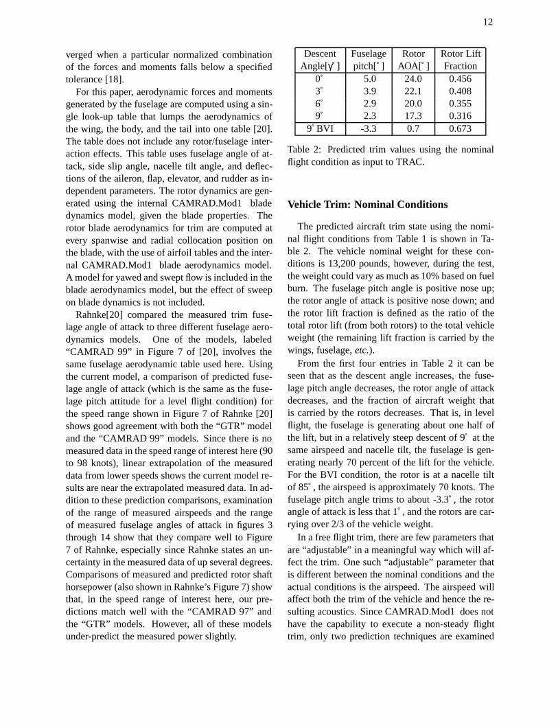
Descent Fuselage Rotor Rotor LiftAngle[γ̊ ] pitch[˚ ] AOA[̊ ] Fraction

0˚ 5.0 24.0 0.4563˚ 3.9 22.1 0.4086˚ 2.9 20.0 0.3559˚ 2.3 17.3 0.316

9˚ BVI -3.3 0.7 0.673

Table 2: Predicted trim values using the nominalflight condition as input to TRAC.

Vehicle Trim: Nominal Conditions

The predicted aircraft trim state using the nomi-nal flight conditions from Table 1 is shown in Ta-ble 2. The vehicle nominal weight for these con-ditions is 13,200 pounds, however, during the test,the weight could vary as much as 10% based on fuelburn. The fuselage pitch angle is positive nose up;the rotor angle of attack is positive nose down; andthe rotor lift fraction is defined as the ratio of thetotal rotor lift (from both rotors) to the total vehicleweight (the remaining lift fraction is carried by thewings, fuselage, etc.).

From the first four entries in Table 2 it can beseen that as the descent angle increases, the fuse-lage pitch angle decreases, the rotor angle of attackdecreases, and the fraction of aircraft weight thatis carried by the rotors decreases. That is, in levelflight, the fuselage is generating about one half ofthe lift, but in a relatively steep descent of 9˚ at thesame airspeed and nacelle tilt, the fuselage is gen-erating nearly 70 percent of the lift for the vehicle.For the BVI condition, the rotor is at a nacelle tiltof 85˚ , the airspeed is approximately 70 knots. Thefuselage pitch angle trims to about -3.3˚ , the rotorangle of attack is less that 1˚ , and the rotors are car-rying over 2/3 of the vehicle weight.

In a free flight trim, there are few parameters thatare “adjustable” in a meaningful way which will af-fect the trim. One such “adjustable” parameter thatis different between the nominal conditions and theactual conditions is the airspeed. The airspeed willaffect both the trim of the vehicle and hence the re-sulting acoustics. Since CAMRAD.Mod1 does nothave the capability to execute a non-steady flighttrim, only two prediction techniques are examined

13

here. The first technique, labeled “Prediction One,”is a standard technique which would be used ina true prediction. Prediction One is executed us-ing only the nominal flight conditions for the air-craft. This nominal condition is used in both theCAMRAD.Mod1 computation and the WOPMODacoustic prediction. The second technique, labeled“Prediction Two,” is designed to examine the effectof aircraft position and orientation on the predic-tion. Since CAMRAD.Mod1 uses only a steadystate trim, the results of Prediction One are used inthe Prediction Two technique. The Prediction Twoacoustics are computed using the optically mea-sured aircraft position (at the retarded time for agiven microphone and time) and the onboard mea-sured orientation of the vehicle (again, at the re-tarded time). These measured quantities are inputto the acoustic analysis, WOPMOD as a function oftime in a quasi-steady manner.

Acoustic Time Histories: Prediction One

The predicted acoustic pressure time historiesfor the level flight and non-BVI descent cases areshown in figures 30 through 33. These are pre-sented in a slightly different format from the mea-sured data. Since these are for nominal conditions,each flight condition is shown as a separate figure.The three rows in each figure are for the centerlinemicrophone (“mic 9”) and the two sideline micro-phones used previously (“mic 6” and “mic 12”). Itcan be seen that in all of these cases, for the center-line microphone, there is only a single pulse. This isbecause the signals from each rotor arrive at the cen-terline microphone at exactly the same time, due tothe symmetry of the nominal condition. Likewise,the signals from the two sideline microphones areidentical also due to the symmetry condition. Thesideline microphone signals, as expected, containthe double pulses.

Overall all the time histories for the level flightand glideslope sweep exhibit the same general char-acter. There are impulsive features, but not BVI asthe aircraft approaches the array. This is consistentwith what was observed in the measured data. Asthe aircraft is overhead, the signal changes to lowfrequency loading noise, which continues as the air-

craft passes the array. Note that there is no broad-band component included in the prediction.

For the BVI condition in figure 34, there is ev-idence of BVI events. However, they are domi-nant primarily in the “5 sec after” overhead plot.The measured data for this case (figure 19) containBVI for all times shown. At times before the air-craft was overhead the measured data contain verystrong, prominent BVI events and less significantBVI events after the aircraft is overhead. Much suc-cess has been reported in comparing predicted withmeasured BVI tiltrotor noise obtained from windtunnel tests [11, 12, 14]. In those tests, the rotorconditions (i.e., rotor thrust, rotor angle of attack,rotor moments, and advance ratio) were all knownand measured. For the flight test, none of theseare known or measured to any degree of accuracy,except the advance ratio. Predicted BVI noise isknown to be sensitive to, and a direct function of,the rotor thrust, rotor angle of attack, and advanceratio.

Flight predictions using TRAC determine the ro-tor thrust, rotor angle of attack, and rotor collective(governor) and longitudinal cyclic settings based onsumming the forces and moments for the entire air-craft. As explained earlier, the aircraft fuselage(wing, body, and tail) aerodynamics are lumped intoone table. The effect of rotor downwash and anyother rotor/fuselage interactional effects are not ac-counted for in this table. The determination of thelift share between the rotor and the fuselage will bein error, particularly for low speed flight. The mag-nitude of the error is not known at this time. How-ever, based on the estimates used for planning twotiltrotor wind tunnel tests (references [12] and [14]),the predicted rotor thrust for this BVI flight condi-tion is about 20% low. TRAC predictions for an iso-lated XV-15 rotor with the higher rotor thrust pro-duce significant BVI events. The main differencebetween these and the predictions made for flight isthe unknown lift share between the body and the ro-tors, which is, to first order, a direct function of thebody table and overall trim procedure within CAM-RAD.Mod1. In order to significantly advance tiltro-tor flight prediction methods, particularly for BVIflight conditions, accurate measurements of the ro-tor state, (i.e., rotor thrust, rotor tip-path-plane an-gle, and aircraft body orientation) must be made

14

available.

LowSPL: Prediction One

Figure 35 shows the integrated LowSPL time his-tory for the level flight condition, along with therange of measured data. (The measured data bandis the minimum and maximum LowSPL values ateach time on the horizontal axis.) It can be seen thatthe overall features are the same as the measureddata shown in figure 22. That is, the level increasesas the aircraft approaches the array, the level peaksapproximately 2 seconds before the aircraft reachesthe array, and the level decreases dramatically afterthe aircraft passes the array. The decrease in pre-dicted levels after the aircraft has passed the array islarger than the measured decrease. The location ofthe peak level is well predicted, but the peak levelitself is underpredicted. The measured data alsoshowed that the peak level for the sideline micro-phones is lower than for the centerline microphone;this same trend is seen in the prediction.

Figure 36 shows the descent cases, including theBVI case. The corresponding measure data can beseen in figure 23. Also on figure 36 is the range ofmeasured data for all of the descent cases. The non-BVI cases show the same trends as the level flightcases and compare in a similar fashion to the mea-sured data. However, the BVI condition does notfollow the same trend as the measured data shownin figure 23, but it does fall with in the measuredband of data for the descent cases.

Figure 37 is the LowSPL contour plot for thelevel flight case for Prediction One. Again, notethat there is only one figure since this prediction isfor the nominal flight condition, which is identicalfor all four of the level flight cases. The predictedLowSPL directivity has the same general features asthe measured directivities shown in figure 24. Thatis, the maximum LowSPL is in front of the vehi-cle, primarily in the plane of the rotor (i.e., 60˚ onthe horizontal axis). The minimum LowSPL noiseis aft of the vehicle, with two “lobes” centered atapproximately �45˚ . The Prediction One LowSPLcontours for the descent cases are shown in figure38. Again, the contours of the first three descentcases have the same general characteristic shape asthe measured data (figure 25). As the descent an-

gle becomes steeper, the maximum LowSPL shiftsslightly forward and the two minima aft of the ve-hicle become more focussed and are moved slightlyoutboard. The predicted BVI case contours also fol-low the same trend as the measured data. That is,the maximum LowSPL is spread over a larger area,extending from directly beneath to far forward ofthe vehicle. Also, both the measured and predicteddata show that the minimum “lobes” are no longerpresent.

Since the primary component of the MidSPL forthese cases is broadband noise, and since there iscurrently no broadband included in the predictions,no predicted results are shown here for the MidSPL.

Acoustic Time Histories: Prediction Two

Figures 39 through 44 are the predicted acous-tic pressure time histories for the level flight anddescent cases. These “Prediction Two” cases usethe exact same loading information from CAM-RAD.Mod1 as in the “Prediction One” cases. How-ever, in the noise computation (WOPMOD), insteadof using observer locations computed from the nom-inal position and orientation of the vehicle and as-suming symmetry, the observer locations are com-puted for each rotor using the optically measuredposition (longitudinal, lateral, and altitude) and on-board measured orientation (yaw, pitch and roll at-titude). As can be seen from these predictions, thesmall changes in vehicle orientation can have a sub-stantial impact on the acoustic pressure time histo-ries. This can be dramatically seen in several fig-ures.

Figure 39 shows the centerline microphone forthe four repeated level flight cases. All the re-sults contain two distinct pulses. In the PredictionOne results, this centerline microphone always hasa single pulse because the rotors are symmetricallyplaced about the microphone. Figure 40 and 41show the predictions for the sideline microphones.Two of the cases have a single pulse for micro-phone 6 while microphone 12 always has two dis-tinct pulses with a variable time between pulses foreach run. Prediction One results for the sideline mi-crophones always show two pulses because the ro-tors are symmetric about the microphone. For all ofthese non-nominal conditions, the problem is now

15

asymmetric. The sensitivity of the acoustic pres-sure time histories to the actual orientation of thevehicle, even when position and orientation pertur-bations are relatively small, was speculated to be theroot cause of the anomalies seen in the measuredtime histories presented earlier. Comparing the Pre-diction One results to the Predictions Two results,this sensitivity is clearly seen to be a factor. Thoughthere are no repeated descent conditions to comparewith, this trend is seen to hold in the descent casesas well in figures 42 through 44.

Though these predictions account for measuredposition and orientation of the vehicle, the mea-sured blade position has not been included since itwas not measured. The predictions show that theacoustic pressure time histories are very sensitive toposition and orientation. Even the measured datashowed that the small differences in distance be-tween sources have a large impact on the acoustictime histories. Since even the azimuthal locationof the blades as a function of time is not known,large differences in blade position are possible be-tween the measured and predicted acoustics. Basedon the double pulses, even distance differences onthe order of a couple of feet can result in drasti-cally different acoustic time histories. Differenceseven as small as those created by the unknown az-imuthal location of the blades can possibly accountfor many of the differences seen in the measured andpredicted acoustic pressure time histories.

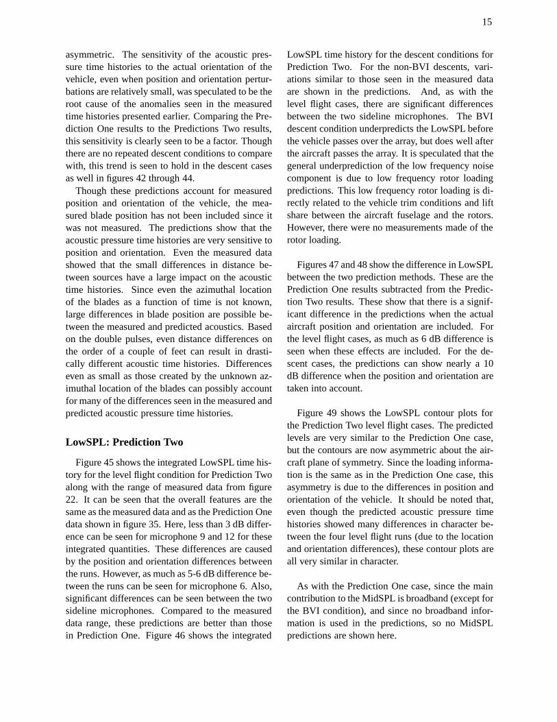
LowSPL: Prediction Two

Figure 45 shows the integrated LowSPL time his-tory for the level flight condition for Prediction Twoalong with the range of measured data from figure22. It can be seen that the overall features are thesame as the measured data and as the Prediction Onedata shown in figure 35. Here, less than 3 dB differ-ence can be seen for microphone 9 and 12 for theseintegrated quantities. These differences are causedby the position and orientation differences betweenthe runs. However, as much as 5-6 dB difference be-tween the runs can be seen for microphone 6. Also,significant differences can be seen between the twosideline microphones. Compared to the measureddata range, these predictions are better than thosein Prediction One. Figure 46 shows the integrated

LowSPL time history for the descent conditions forPrediction Two. For the non-BVI descents, vari-ations similar to those seen in the measured dataare shown in the predictions. And, as with thelevel flight cases, there are significant differencesbetween the two sideline microphones. The BVIdescent condition underpredicts the LowSPL beforethe vehicle passes over the array, but does well afterthe aircraft passes the array. It is speculated that thegeneral underprediction of the low frequency noisecomponent is due to low frequency rotor loadingpredictions. This low frequency rotor loading is di-rectly related to the vehicle trim conditions and liftshare between the aircraft fuselage and the rotors.However, there were no measurements made of therotor loading.

Figures 47 and 48 show the difference in LowSPLbetween the two prediction methods. These are thePrediction One results subtracted from the Predic-tion Two results. These show that there is a signif-icant difference in the predictions when the actualaircraft position and orientation are included. Forthe level flight cases, as much as 6 dB difference isseen when these effects are included. For the de-scent cases, the predictions can show nearly a 10dB difference when the position and orientation aretaken into account.

Figure 49 shows the LowSPL contour plots forthe Prediction Two level flight cases. The predictedlevels are very similar to the Prediction One case,but the contours are now asymmetric about the air-craft plane of symmetry. Since the loading informa-tion is the same as in the Prediction One case, thisasymmetry is due to the differences in position andorientation of the vehicle. It should be noted that,even though the predicted acoustic pressure timehistories showed many differences in character be-tween the four level flight runs (due to the locationand orientation differences), these contour plots areall very similar in character.

As with the Prediction One case, since the maincontribution to the MidSPL is broadband (except forthe BVI condition), and since no broadband infor-mation is used in the predictions, so no MidSPLpredictions are shown here.

16

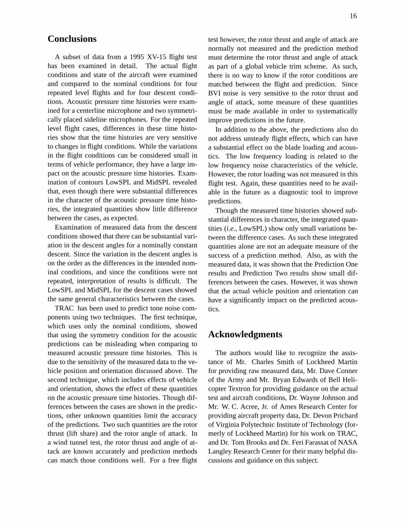
Conclusions

A subset of data from a 1995 XV-15 flight testhas been examined in detail. The actual flightconditions and state of the aircraft were examinedand compared to the nominal conditions for fourrepeated level flights and for four descent condi-tions. Acoustic pressure time histories were exam-ined for a centerline microphone and two symmetri-cally placed sideline microphones. For the repeatedlevel flight cases, differences in these time histo-ries show that the time histories are very sensitiveto changes in flight conditions. While the variationsin the flight conditions can be considered small interms of vehicle performance, they have a large im-pact on the acoustic pressure time histories. Exam-ination of contours LowSPL and MidSPL revealedthat, even though there were substantial differencesin the character of the acoustic pressure time histo-ries, the integrated quantities show little differencebetween the cases, as expected.

Examination of measured data from the descentconditions showed that there can be substantial vari-ation in the descent angles for a nominally constantdescent. Since the variation in the descent angles ison the order as the differences in the intended nom-inal conditions, and since the conditions were notrepeated, interpretation of results is difficult. TheLowSPL and MidSPL for the descent cases showedthe same general characteristics between the cases.

TRAC has been used to predict tone noise com-ponents using two techniques. The first technique,which uses only the nominal conditions, showedthat using the symmetry condition for the acousticpredictions can be misleading when comparing tomeasured acoustic pressure time histories. This isdue to the sensitivity of the measured data to the ve-hicle position and orientation discussed above. Thesecond technique, which includes effects of vehicleand orientation, shows the effect of these quantitieson the acoustic pressure time histories. Though dif-ferences between the cases are shown in the predic-tions, other unknown quantities limit the accuracyof the predictions. Two such quantities are the rotorthrust (lift share) and the rotor angle of attack. Ina wind tunnel test, the rotor thrust and angle of at-tack are known accurately and prediction methodscan match those conditions well. For a free flight

test however, the rotor thrust and angle of attack arenormally not measured and the prediction methodmust determine the rotor thrust and angle of attackas part of a global vehicle trim scheme. As such,there is no way to know if the rotor conditions arematched between the flight and prediction. SinceBVI noise is very sensitive to the rotor thrust andangle of attack, some measure of these quantitiesmust be made available in order to systematicallyimprove predictions in the future.

In addition to the above, the predictions also donot address unsteady flight effects, which can havea substantial effect on the blade loading and acous-tics. The low frequency loading is related to thelow frequency noise characteristics of the vehicle.However, the rotor loading was not measured in thisflight test. Again, these quantities need to be avail-able in the future as a diagnostic tool to improvepredictions.

Though the measured time histories showed sub-stantial differences in character, the integrated quan-tities (i.e., LowSPL) show only small variations be-tween the difference cases. As such these integratedquantities alone are not an adequate measure of thesuccess of a prediction method. Also, as with themeasured data, it was shown that the Prediction Oneresults and Prediction Two results show small dif-ferences between the cases. However, it was shownthat the actual vehicle position and orientation canhave a significantly impact on the predicted acous-tics.

Acknowledgments

The authors would like to recognize the assis-tance of Mr. Charles Smith of Lockheed Martinfor providing raw measured data, Mr. Dave Connerof the Army and Mr. Bryan Edwards of Bell Heli-copter Textron for providing guidance on the actualtest and aircraft conditions, Dr. Wayne Johnson andMr. W. C. Acree, Jr. of Ames Research Center forproviding aircraft property data, Dr. Devon Prichardof Virginia Polytechnic Institute of Technology (for-merly of Lockheed Martin) for his work on TRAC,and Dr. Tom Brooks and Dr. Feri Farassat of NASALangley Research Center for their many helpful dis-cussions and guidance on this subject.

17

References

[1] Marcolini, M.A., Burley, C.L., Conner, D.A.,Acree, Jr., C.W., “Overview of Noise Re-duction Technology of the NASA ShortHaul (Civil Tiltrotor) Program,” SAE Paper962273, International Powered Lift Confer-ence, Jupiter, FL, November 8-10, 1996.

[2] Edwards, B.D., “XV-15 Tiltrotor AircraftNoise Characteristics,” 46th AHS Annual Fo-rum, Fort Worth, TX, May 9-11, 1990.

[3] Conner, D.A. and Wellman, J.B., “HoverAcoustic Characteristics of the XV-15 withAdvanced Technology Blades,” AIAA Journalof Aircraft, Vol. 31, No. 4, 1994.

[4] Conner, D.A., Marcolini, M.A., Edwards,B.D., Brieger, J.T., “XV-15 Tiltrotor LowNoise Terminal Area Operations,” 53rd AHSAnnual Forum, Virginia Beach, VA, April-May 1997.

[5] Edwards, B.D., “XV-15 Low-Noise TerminalArea Operations Testing,” NASA CR-1998-206946, February 1998.

[6] Hoad, D.R., Conner, D.A., Rutledge, C.K.,“Acoustic Flight Test Experience With theXV-15 Tiltrotor Aircraft With the AdvancedTechnology Blade (ATB),” 14th DGLR/AIAAAeroacoustics Conference, Aachen, Germany,May 1992.

[7] Marcolini, M.A., Conner, D.A., Brieger, J.T.,Becker, L.E., Smith, C.D., “Noise Character-istics of a Model Tiltrotor,” 51st AHS AnnualForum, Fort Worth, TX, May 1995.

[8] Liu, S.R., Brieger, J., Peryea, M., “ModelTiltrotor Flow Field/Turbulence IngestionNoise Experiment and Prediction,” 54th AHSAnnual Forum, Washington, D.C, May 1998.

[9] Polak, D.R. and George, A.R., “Flowfield andAcoustic Measurements From a Model Tiltro-tor in Hover,” AIAA Journal of Aircraft, Vol.35, No. 6, December 1998.

[10] Prichard, D.S., Boyd, Jr., D.D., BurleyC.L., “NASA/Langley’s CFD-Based BVIRotor Noise Prediction System: (RO-TONET/FPRBVI) An Introduction and User’sGuide,” NASA TM 109147, November 1994.

[11] Brooks, T.F., Boyd, Jr., D.D., Burley,C.L., Jolly, Jr., R.J., “Aeroacoustic Codesfor Rotor Harmonic and BVI Noise-CAMRAD.Mod1/HIRES,” AIAA PaperNo. 96-1735, 1996.

[12] Burley, C.L., Marcolini, M.A., Brooks, T.F.,Brand, A.G., Conner, D.A., “Tiltrotor Aeroa-coustic Code (TRAC) Predictions and Com-parison with Measurements,” 52nd AHS An-nual Forum, Washington, D.C., June 4-6,1996.

[13] Boyd, Jr., D.D., Brooks, T.F., Burley,C.L., Jolly, Jr., J.R., “Aeroacoustic Codesfor Rotor Harmonic and BVI Noise-CAMRAD.Mod1/HIRES: Methodologyand User’s Manual,” NASA TM 110297,March 1998.

[14] Burley, C.L., Brooks, T.F., Marcolini, M.A.,“Tiltrotor Aeroacoustic Code (TRAC) Predic-tion Assessment and Initial Comparison withTRAM Test Data,” 25th European RotorcraftForum, Rome, Italy, September 1999.

[15] Prichard, D.S., “Initial Tiltrotor Aeroacous-tic Code (TRAC) Predictions for the XV-15Flight Vehicle and Comparison with FlightMeasurements,” 56th AHS Annual Forum,Virginia Beach, VA, May 2-4, 2000.

[16] JanakiRam, R.D., Khan, H., “Predictionand Validation of Helicopter Descent FlyoverNoise,” 56th AHS Annual Forum, VirginiaBeach, VA, May 2-4, 2000.

[17] Brooks, T.F., Boyd, Jr., D.D., Burley,C.L., Jolly, Jr., R.J., “Aeroacoustic Codesfor Rotor Harmonic and BVI Noise-CAMRAD.Mod1/HIRES,” Journal of theAmerican Helicopter Society, April 2000.

[18] Johnson, W., “A Comprehensive AnalyticalModel of Rotorcraft Aerodynamics and Dy-

18

namics, Part I: Analysis Development,” NASATM 81182, June 1980.

[19] Johnson, W., “A Comprehensive AnalyticalModel of Rotorcraft Aerodynamics and Dy-namics, Part II: User’s Manual,” NASA TM81183, July 1980.

[20] Rahnke, C., “XV-15 Aerodynamic Model andBlade Tip Acoustic Study,” Bell Report No.699-099-507, August 12, 1999.

[21] Beddoes, T.S., “A Near Wake DynamicModel,” Proceedings of the AHS SpecialistsMeeting on Aerodynamics and Aeroacoustics,February 1987.

[22] Beddoes, T.S., “Two and Three DimensionalIndicial Methods for Rotor Dynamic Air-loads,” AHS National Specialists Meeting onRotorcraft Dynamics, November 1989.

[23] Beddoes, T.S., Leishman, J.G., “A Gener-alised Model for Airfoil Unsteady Aerody-namics Using the Indicial Method,” 42nd AHSAnnual Forum, June 1986.

[24] Beddoes, T.S., Leishman, J.G., “A Semi-Empirical Model for Dynamic Stall,” Jour-nal of the American Helicopter Society, July1989.

[25] Brentner, K.S., “Prediction of Helicopter Ro-tor Discrete Frequency Noise,” NASA TM87721, October 1986.

[26] Brooks, T.F., Jolly, Jr., R.J., Marcolini, M.A.,“Helicopter Main-Rotor Noise: Determinationof Source Contributions Using Scaled ModelData,” NASA TP 2825, August 1988.

[27] Burley, C.L., Brooks, T.F., Splettstoesser,W.R., Schultz, K.-J., Kube, R., Bucholtz, H.,Wagner, W., Weitemeyer, W., “Blade WakeInteraction Noise for a BO-105 Model MainRotor,” AHS Technical Specialists’ MeetingFor Rotorcraft Acoustics and Aerodynamics,Williamsburg, VA, October, 28-30, 1997.

[28] “Tilt Rotor Research Aircraft Familiariza-tion Document,” NASA TMX-62407, January1975.

[29] Hardin, J.C., “Introduction to Time SeriesAnalysis,” NASA Reference Publication 1145,Second Printing, November 1990.

[30] Bendat, J.S., Piersol, A.G., “Engineering Ap-plications of Correlation and Spectral Analy-sis,” pp. 75-76, A Wiley-Interscience Publica-tion, John Wiley & Sons, Inc., ISBN 0-471-05887-4, 1980.

[31] Brieger, J.T., Maisel, M.D., Gerdes, R., “Ex-ternal Noise Evaluation of the XV-15 TiltrotorAircraft,” AHS National Specialists’ Meetingon Aerodynamic and Aeroacoustics, Arling-ton, TX, February 25-27, 1987.

19

CAMRAD.Mod1

IPP

WOPMOD

HIRES

Figure 1: Schematic of TRAC used in this paper.

Late

ralD

ista

nce

[ft]

-2500

-2000

-1500

-1000

-500

0

500

1000

1500

2000

2500

Nominal Flight Path

microphone 1

microphone 17

microphone 12

microphone 6

microphone 9

69.5’143.4’227.5’330.6’469.6’682.4’

1082.5’

2234.5’

0.0’

Figure 2: Microphone layout for Phase I part of1995 flight test.

time [sec]

Airs

peed

[kno

ts]

-20 -10 0 10 2060

65

70

75

80

85

90

95

100

time [sec]

Airs

peed

[kno

ts]

-20 -10 0 10 2060

65

70

75

80

85

90

95

100

time [sec]

Airs

peed

[kno

ts]

-20 -10 0 10 2060

65

70

75

80

85

90

95

100nominal

run 1

run 2

run 3

run 4Level Flights

time [sec]

Airs

peed

[kno

ts]

-20 -10 0 10 2060

65

70

75

80

85

90

95

100

Figure 3: Measured airspeed for level flight runs 1through 4 (the aircraft is overhead at t= 0).

time [sec]

Airs

peed

[kno

ts]

-20 -10 0 10 2060

65

70

75

80

85

90

95

100

time [sec]

Airs

peed

[kno

ts]

-20 -10 0 10 2060

65

70

75

80

85

90

95

100

time [sec]

Airs

peed

[kno

ts]

-20 -10 0 10 2060

65

70

75

80

85

90

95

100

time [sec]

Airs

peed

[kno

ts]

-20 -10 0 10 2060

65

70

75

80

85

90

95

100nominal 90 knots

3° Descent

6° Descent

9° Descent

Descent Cases

nominal 70 knots 9° Descent BVI

Figure 4: Measured airspeed for descent flight con-ditions (the aircraft is overhead at t= 0).

20

time [sec]

Alti

tud

e[f

t]

-20 -10 0 10 200

100

200

300

400

500

600

700

800

900

1000

time [sec]

Alti

tud

e[f

t]

-20 -10 0 10 200

100

200

300

400

500

600

700

800

900

1000

time [sec]

Alti

tud

e[f

t]

-20 -10 0 10 200

100

200

300

400

500

600

700

800

900

1000

time [sec]

Alti

tud

e[f

t]

-20 -10 0 10 200

100

200

300

400

500

600

700

800

900

1000nominal

run 1

run 2

run 3

run 4Level Flights

Figure 5: Measured altitude for level flight runs 1through 4 (the aircraft is overhead at t= 0).

time [sec]

Alti

tud

e[f

t]

-20 -10 0 10 200

100

200

300

400

500

600

700

800

900

1000

time [sec]

Alti

tud

e[f

t]

-20 -10 0 10 200

100

200

300

400

500

600

700

800

900

1000

time [sec]

Alti

tud

e[f

t]

-20 -10 0 10 200

100

200

300

400

500

600

700

800

900

1000

time [sec]

Alti

tud

e[f

t]

-20 -10 0 10 200

100

200

300

400

500

600

700

800

900

1000nominal 3° Descent

nominal 6° Descent

3° Descent

6° Descent

Descent Cases

nominal 9° Descent 9° Descent

9° Descent BVI

Figure 6: Measured altitude for descent flight con-ditions (the aircraft is overhead at t= 0).

time [sec]

Lat

eral

Po

sitio

n[f

t]

-20 -10 0 10 20-50

-40

-30

-20

-10

0

10

20

30

40

50

time [sec]

Lat

eral

Po

sitio

n[f

t]

-20 -10 0 10 20-50

-40

-30

-20

-10

0

10

20

30

40

50

time [sec]

Lat

eral

Po

sitio

n[f

t]

-20 -10 0 10 20-50

-40

-30

-20

-10

0

10

20

30

40

50

time [sec]

Lat

eral

Po

sitio

n[f

t]

-20 -10 0 10 20-50

-40

-30

-20

-10

0

10

20

30

40

50nominal

run 1

run 2

run 3

run 4Level Flights

Figure 7: Measured lateral position for level flightruns 1 through 4 (the aircraft is overhead at t= 0).

time [sec]

Lat

eral

Po

sitio

n[f

t]

-20 -10 0 10 20-50

-40

-30

-20

-10

0

10

20

30

40

50

time [sec]

Lat

eral

Po

sitio

n[f

t]

-20 -10 0 10 20-50

-40

-30

-20

-10

0

10

20

30

40

50

time [sec]

Lat

eral

Po

sitio

n[f

t]

-20 -10 0 10 20-50

-40

-30

-20

-10

0

10

20

30

40

50

time [sec]

Lat

eral

Po

sitio

n[f

t]

-20 -10 0 10 20-50

-40

-30

-20

-10

0

10

20

30

40

50nominal

3° Descent

6° Descent

9° Descent

Descent Cases

9° Descent BVI

Figure 8: Measured lateral position for descentflight conditions (the aircraft is overhead at t= 0).

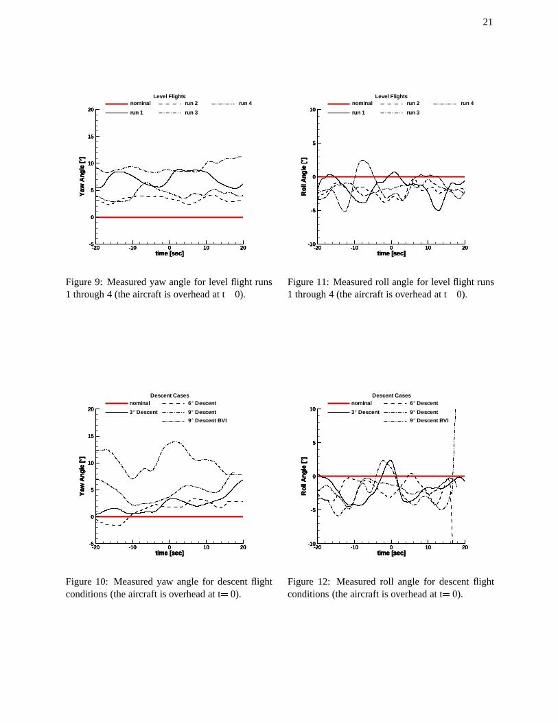
21

nominal

run 1

run 2

run 3

run 4Level Flights

time [sec]

Yaw

Ang

le[°

]

-20 -10 0 10 20-5

0

5

10

15

20

time [sec]

Yaw

Ang

le[°

]

-20 -10 0 10 20-5

0

5

10

15

20

time [sec]

Yaw

Ang

le[°

]

-20 -10 0 10 20-5

0

5

10

15

20

time [sec]

Yaw

Ang

le[°

]

-20 -10 0 10 20-5

0

5

10

15

20

Figure 9: Measured yaw angle for level flight runs1 through 4 (the aircraft is overhead at t= 0).

time [sec]

Yaw

Ang

le[°

]

-20 -10 0 10 20-5

0

5

10

15

20

time [sec]

Yaw

Ang

le[°

]

-20 -10 0 10 20-5

0

5

10

15

20

time [sec]

Yaw

Ang

le[°

]

-20 -10 0 10 20-5

0

5

10

15

20

time [sec]

Yaw

Ang

le[°

]

-20 -10 0 10 20-5

0

5

10

15

20nominal

3° Descent

6° Descent

9° Descent

Descent Cases

9° Descent BVI

Figure 10: Measured yaw angle for descent flightconditions (the aircraft is overhead at t= 0).

time [sec]

Rol

lAng

le[°

]

-20 -10 0 10 20-10

-5

0

5

10

time [sec]

Rol

lAng

le[°

]

-20 -10 0 10 20-10

-5

0

5

10

time [sec]

Rol

lAng

le[°

]

-20 -10 0 10 20-10

-5

0

5

10

time [sec]

Rol

lAng

le[°

]

-20 -10 0 10 20-10

-5

0

5

10nominal

run 1

run 2

run 3

run 4Level Flights

Figure 11: Measured roll angle for level flight runs1 through 4 (the aircraft is overhead at t= 0).

time [sec]

Rol

lAng

le[°

]

-20 -10 0 10 20-10

-5

0

5

10

time [sec]

Rol

lAng

le[°

]

-20 -10 0 10 20-10

-5

0

5

10

time [sec]

Rol

lAng

le[°

]

-20 -10 0 10 20-10

-5

0

5

10

time [sec]

Rol

lAng

le[°

]

-20 -10 0 10 20-10

-5

0

5

10nominal

3° Descent

6° Descent

9° Descent

Descent Cases

9° Descent BVI

Figure 12: Measured roll angle for descent flightconditions (the aircraft is overhead at t= 0).

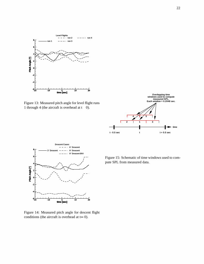
22

time [sec]

Pitc

hA

ngle

[°]

-20 -10 0 10 20-6

-4

-2

0

2

4

6

8

time [sec]

Pitc

hA

ngle

[°]

-20 -10 0 10 20-6

-4

-2

0

2

4

6

8

time [sec]

Pitc

hA

ngle

[°]

-20 -10 0 10 20-6

-4

-2

0

2

4

6

8

time [sec]

Pitc

hA

ngle

[°]

-20 -10 0 10 20-6

-4

-2

0

2

4

6

8 run 1

run 2

run 3

run 4Level Flights

Figure 13: Measured pitch angle for level flight runs1 through 4 (the aircraft is overhead at t= 0).

time [sec]

Pitc

hA

ngle

[°]

-20 -10 0 10 20-6

-4

-2

0

2

4

6

8

time [sec]

Pitc

hA

ngle

[°]

-20 -10 0 10 20-6

-4

-2

0

2

4

6

8

time [sec]

Pitc

hA

ngle

[°]

-20 -10 0 10 20-6

-4

-2

0

2

4

6

8

time [sec]

Pitc

hA

ngle

[°]

-20 -10 0 10 20-6

-4

-2

0

2

4

6

8 3° Descent

6° Descent

9° Descent

Descent Cases

9° Descent BVI

Figure 14: Measured pitch angle for descent flightconditions (the aircraft is overhead at t= 0).

t t + 0.5 sect - 0.5 sec

12 3

4 5

time

Overlapping timewindows used to compute

measured SPL.Each window = 0.2048 sec.

Figure 15: Schematic of time windows used to com-pute SPL from measured data.

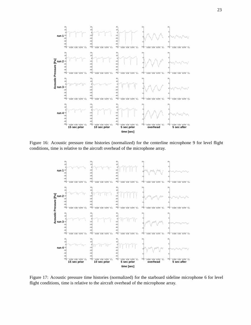
23

0 0.025 0.05 0.075 0.1-50

-40

-30

-20

-10

0

10

20

0 0.025 0.05 0.075 0.1-50

-40

-30

-20

-10

0

10

20

0 0.025 0.05 0.075 0.1-50

-40

-30

-20

-10

0

10

20

0 0.025 0.05 0.075 0.1-10

-5

0

5

10

0 0.025 0.05 0.075 0.1-10

-5

0

5

10

0 0.025 0.05 0.075 0.1-50

-40

-30

-20

-10

0

10

20

0 0.025 0.05 0.075 0.1-50

-40

-30

-20

-10

0

10

20

0 0.025 0.05 0.075 0.1-50

-40

-30

-20

-10

0

10

20

0 0.025 0.05 0.075 0.1-10

-5

0

5

10

0 0.025 0.05 0.075 0.1-10

-5

0

5

10

0 0.025 0.05 0.075 0.1-50

-40

-30

-20

-10

0

10

20

0 0.025 0.05 0.075 0.1-50

-40

-30

-20

-10

0

10

20

0 0.025 0.05 0.075 0.1-50

-40

-30

-20

-10

0

10

20

0 0.025 0.05 0.075 0.1-10

-5

0

5

10

0 0.025 0.05 0.075 0.1-10

-5

0

5

10

0 0.025 0.05 0.075 0.1-50

-40

-30

-20

-10

0

10

20

0 0.025 0.05 0.075 0.1-50

-40

-30

-20

-10

0

10

20

0 0.025 0.05 0.075 0.1-50

-40

-30

-20

-10

0

10

20

0 0.025 0.05 0.075 0.1-10

-5

0

5

10

0 0.025 0.05 0.075 0.1-10

-5

0

5

10

time [sec]

Aco

ustic

Pre

ssur

e[P

a]

15 sec prior 10 sec prior 5 sec prior overhead 5 sec after

run 4

run 3

run 2

run 1

Figure 16: Acoustic pressure time histories (normalized) for the centerline microphone 9 for level flightconditions, time is relative to the aircraft overhead of the microphone array.

0 0.025 0.05 0.075 0.1-50

-40

-30

-20

-10

0

10

20

0 0.025 0.05 0.075 0.1-50

-40

-30

-20

-10

0

10

20

0 0.025 0.05 0.075 0.1-50

-40

-30

-20

-10

0

10

20

0 0.025 0.05 0.075 0.1-10

-5

0

5

10

0 0.025 0.05 0.075 0.1-10

-5

0

5

10

0 0.025 0.05 0.075 0.1-50

-40

-30

-20

-10

0

10

20

0 0.025 0.05 0.075 0.1-50

-40

-30

-20

-10

0

10

20

0 0.025 0.05 0.075 0.1-50

-40

-30

-20

-10

0

10

20

0 0.025 0.05 0.075 0.1-10

-5

0

5

10

0 0.025 0.05 0.075 0.1-10

-5

0

5

10

0 0.025 0.05 0.075 0.1-50

-40

-30

-20

-10

0

10

20

0 0.025 0.05 0.075 0.1-50

-40

-30

-20

-10

0

10

20

0 0.025 0.05 0.075 0.1-50

-40

-30

-20

-10

0

10

20

0 0.025 0.05 0.075 0.1-10

-5

0

5

10

0 0.025 0.05 0.075 0.1-10

-5

0

5

10

0 0.025 0.05 0.075 0.1-50

-40

-30

-20

-10

0

10

20

0 0.025 0.05 0.075 0.1-50

-40

-30

-20

-10

0

10

20

0 0.025 0.05 0.075 0.1-50

-40

-30

-20

-10

0

10

20

0 0.025 0.05 0.075 0.1-10

-5

0

5

10

0 0.025 0.05 0.075 0.1-10

-5

0

5

10

time [sec]

Aco

ustic

Pre

ssur

e[P

a]

15 sec prior 10 sec prior 5 sec prior overhead 5 sec after

run 4

run 3

run 2

run 1

Figure 17: Acoustic pressure time histories (normalized) for the starboard sideline microphone 6 for levelflight conditions, time is relative to the aircraft overhead of the microphone array.

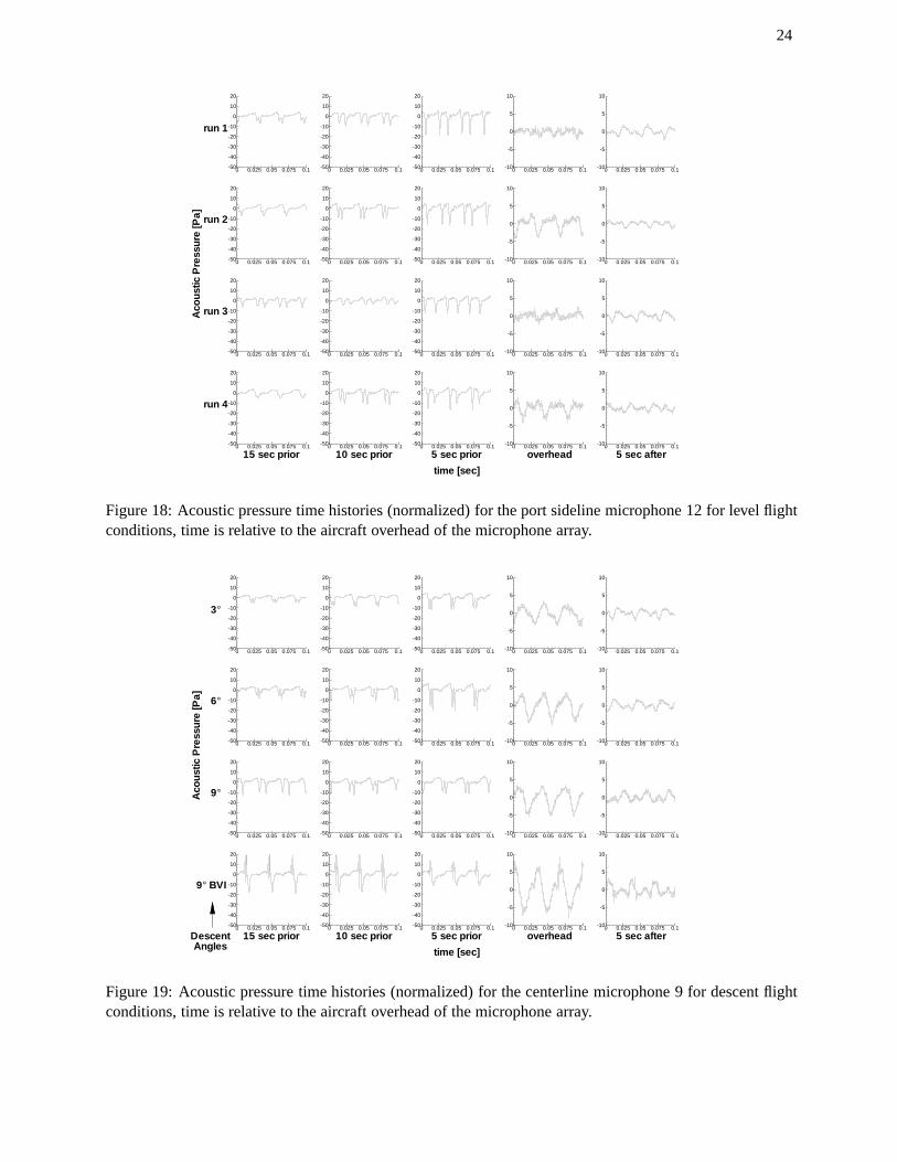
24

0 0.025 0.05 0.075 0.1-50

-40

-30

-20

-10

0

10

20

0 0.025 0.05 0.075 0.1-50

-40

-30

-20

-10

0

10

20

0 0.025 0.05 0.075 0.1-50

-40

-30

-20

-10

0

10

20

0 0.025 0.05 0.075 0.1-10

-5

0

5

10

0 0.025 0.05 0.075 0.1-10

-5

0

5

10

0 0.025 0.05 0.075 0.1-50

-40

-30

-20

-10

0

10

20

0 0.025 0.05 0.075 0.1-50

-40

-30

-20

-10

0

10

20

0 0.025 0.05 0.075 0.1-50

-40

-30

-20

-10

0

10

20

0 0.025 0.05 0.075 0.1-10

-5

0

5

10

0 0.025 0.05 0.075 0.1-10

-5

0

5

10

0 0.025 0.05 0.075 0.1-50

-40

-30

-20

-10

0

10

20

0 0.025 0.05 0.075 0.1-50

-40

-30

-20

-10

0

10

20

0 0.025 0.05 0.075 0.1-50

-40

-30

-20

-10

0

10

20

0 0.025 0.05 0.075 0.1-10

-5

0

5

10

0 0.025 0.05 0.075 0.1-10

-5

0

5

10

0 0.025 0.05 0.075 0.1-50

-40

-30

-20

-10

0

10

20

0 0.025 0.05 0.075 0.1-50

-40

-30

-20

-10

0

10

20

0 0.025 0.05 0.075 0.1-50

-40

-30

-20

-10

0

10

20

0 0.025 0.05 0.075 0.1-10

-5

0

5

10

0 0.025 0.05 0.075 0.1-10

-5

0

5

10

time [sec]

Aco

ustic

Pre

ssur

e[P

a]

15 sec prior 10 sec prior 5 sec prior overhead 5 sec after

run 4

run 3

run 2

run 1

Figure 18: Acoustic pressure time histories (normalized) for the port sideline microphone 12 for level flightconditions, time is relative to the aircraft overhead of the microphone array.

0 0.025 0.05 0.075 0.1-50

-40

-30

-20

-10

0

10

20

0 0.025 0.05 0.075 0.1-50

-40

-30

-20

-10

0

10

20

0 0.025 0.05 0.075 0.1-50

-40

-30

-20

-10

0

10

20

0 0.025 0.05 0.075 0.1-10

-5

0

5

10

0 0.025 0.05 0.075 0.1-10

-5

0

5

10

0 0.025 0.05 0.075 0.1-50

-40

-30

-20

-10

0

10

20

0 0.025 0.05 0.075 0.1-50

-40

-30

-20

-10

0

10

20

0 0.025 0.05 0.075 0.1-50

-40

-30

-20

-10

0

10

20

0 0.025 0.05 0.075 0.1-10

-5

0

5

10

0 0.025 0.05 0.075 0.1-10

-5

0

5

10

0 0.025 0.05 0.075 0.1-50

-40

-30

-20

-10

0

10

20

0 0.025 0.05 0.075 0.1-50

-40

-30

-20

-10

0

10

20

0 0.025 0.05 0.075 0.1-50

-40

-30

-20

-10

0

10

20

0 0.025 0.05 0.075 0.1-10

-5

0

5

10

0 0.025 0.05 0.075 0.1-10

-5

0

5

10

0 0.025 0.05 0.075 0.1-50

-40

-30

-20

-10

0

10

20

0 0.025 0.05 0.075 0.1-50

-40

-30

-20

-10

0

10

20

0 0.025 0.05 0.075 0.1-50

-40

-30

-20

-10

0

10

20

0 0.025 0.05 0.075 0.1-10

-5

0

5

10

0 0.025 0.05 0.075 0.1-10

-5

0

5

10

time [sec]

Aco

ustic

Pre

ssur

e[P

a]

15 sec prior 10 sec prior 5 sec prior overhead 5 sec after

9° BVI

9°

6°

3°

DescentAngles

Figure 19: Acoustic pressure time histories (normalized) for the centerline microphone 9 for descent flightconditions, time is relative to the aircraft overhead of the microphone array.

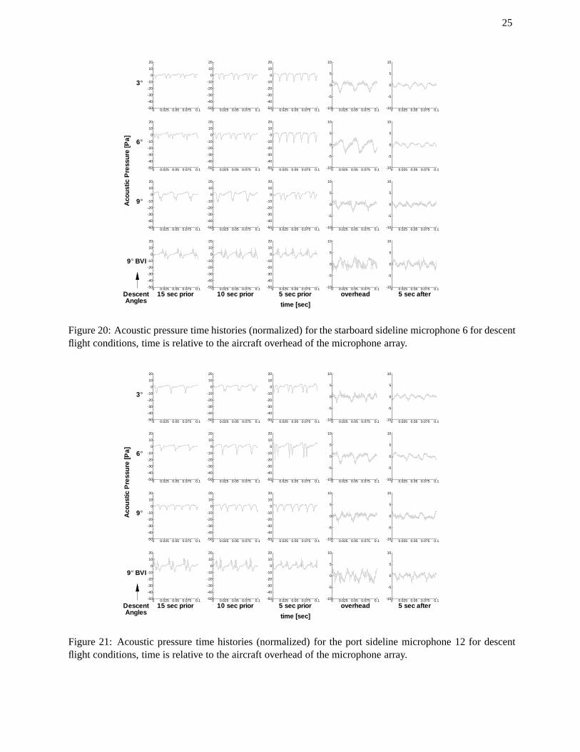
25

0 0.025 0.05 0.075 0.1-50

-40

-30

-20

-10

0

10

20

0 0.025 0.05 0.075 0.1-50

-40

-30

-20

-10

0

10

20

0 0.025 0.05 0.075 0.1-50

-40

-30

-20

-10

0

10

20

0 0.025 0.05 0.075 0.1-10

-5

0

5

10

0 0.025 0.05 0.075 0.1-10

-5

0

5

10

0 0.025 0.05 0.075 0.1-50

-40

-30

-20

-10

0

10

20

0 0.025 0.05 0.075 0.1-50

-40

-30

-20

-10

0

10

20

0 0.025 0.05 0.075 0.1-50

-40

-30

-20

-10

0

10

20

0 0.025 0.05 0.075 0.1-10

-5

0

5

10

0 0.025 0.05 0.075 0.1-10

-5

0

5

10

0 0.025 0.05 0.075 0.1-50

-40

-30

-20

-10

0

10

20

0 0.025 0.05 0.075 0.1-50

-40

-30

-20

-10

0

10

20

0 0.025 0.05 0.075 0.1-50

-40

-30

-20

-10

0

10

20

0 0.025 0.05 0.075 0.1-10

-5

0

5

10

0 0.025 0.05 0.075 0.1-10

-5

0

5

10

0 0.025 0.05 0.075 0.1-50

-40

-30

-20

-10

0

10

20

0 0.025 0.05 0.075 0.1-50

-40

-30

-20

-10

0

10

20

0 0.025 0.05 0.075 0.1-50

-40

-30

-20

-10

0

10

20

0 0.025 0.05 0.075 0.1-10

-5

0

5

10

0 0.025 0.05 0.075 0.1-10

-5

0

5

10

time [sec]

Aco

ustic

Pre

ssur

e[P

a]

15 sec prior 10 sec prior 5 sec prior overhead 5 sec after

9° BVI

9°

6°

3°

DescentAngles

Figure 20: Acoustic pressure time histories (normalized) for the starboard sideline microphone 6 for descentflight conditions, time is relative to the aircraft overhead of the microphone array.

0 0.025 0.05 0.075 0.1-50

-40

-30

-20

-10

0

10

20

0 0.025 0.05 0.075 0.1-50

-40

-30

-20

-10

0

10

20

0 0.025 0.05 0.075 0.1-50

-40

-30

-20

-10

0

10

20

0 0.025 0.05 0.075 0.1-10

-5

0

5

10

0 0.025 0.05 0.075 0.1-10

-5

0

5

10

0 0.025 0.05 0.075 0.1-50

-40

-30

-20

-10

0

10

20

0 0.025 0.05 0.075 0.1-50

-40

-30

-20

-10

0

10

20

0 0.025 0.05 0.075 0.1-50

-40

-30

-20

-10

0

10

20

0 0.025 0.05 0.075 0.1-10

-5

0

5

10

0 0.025 0.05 0.075 0.1-10

-5

0

5

10

0 0.025 0.05 0.075 0.1-50

-40

-30

-20

-10

0

10

20

0 0.025 0.05 0.075 0.1-50

-40

-30

-20

-10

0

10

20

0 0.025 0.05 0.075 0.1-50

-40

-30

-20

-10

0

10

20

0 0.025 0.05 0.075 0.1-10

-5

0

5

10

0 0.025 0.05 0.075 0.1-10

-5

0

5

10

0 0.025 0.05 0.075 0.1-50

-40

-30

-20

-10

0

10

20

0 0.025 0.05 0.075 0.1-50

-40

-30

-20

-10

0

10

20

0 0.025 0.05 0.075 0.1-50

-40

-30

-20

-10

0

10

20

0 0.025 0.05 0.075 0.1-10

-5

0

5

10

0 0.025 0.05 0.075 0.1-10

-5

0

5

10

time [sec]

Aco

ustic

Pre

ssur

e[P

a]

15 sec prior 10 sec prior 5 sec prior overhead 5 sec after

9° BVI

9°

6°

3°

DescentAngles

Figure 21: Acoustic pressure time histories (normalized) for the port sideline microphone 12 for descentflight conditions, time is relative to the aircraft overhead of the microphone array.

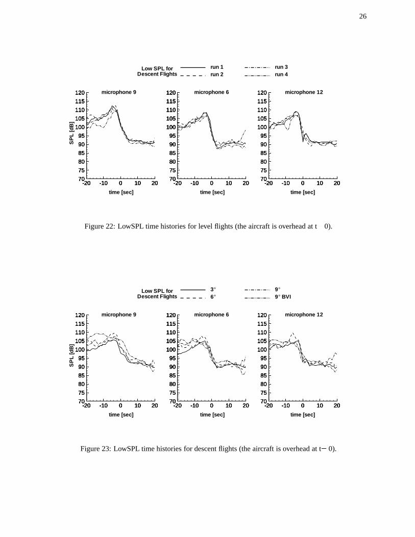
26

-20 -10 0 10 2070

75

80

85

90

95

100

105

110

115

120

-20 -10 0 10 2070

75

80

85

90

95

100

105

110

115

120

-20 -10 0 10 2070

75

80

85

90

95

100

105

110

115

120

-20 -10 0 10 2070

75

80

85

90

95

100

105

110

115

120

-20 -10 0 10 2070

75

80

85

90

95

100

105

110

115

120

-20 -10 0 10 2070

75

80

85

90

95

100

105

110

115

120

-20 -10 0 10 2070

75

80

85

90

95

100

105

110

115

120

-20 -10 0 10 2070

75

80

85

90

95

100

105

110

115

120

-20 -10 0 10 2070

75

80

85

90

95

100

105

110

115

120

-20 -10 0 10 2070

75

80

85

90

95

100

105

110

115

120

-20 -10 0 10 2070

75

80

85

90

95

100

105

110

115

120

-20 -10 0 10 2070

75

80

85

90

95

100

105

110

115

120

time [sec] time [sec] time [sec]

SP

L[d

B]

microphone 9 microphone 6 microphone 12

Low SPL forDescent Flights

run 1run 2

run 3run 4

Figure 22: LowSPL time histories for level flights (the aircraft is overhead at t= 0).

-20 -10 0 10 2070

75

80

85

90

95

100

105

110

115

120

-20 -10 0 10 2070

75

80

85

90

95

100

105

110

115

120

-20 -10 0 10 2070

75

80

85

90

95

100

105

110

115

120

-20 -10 0 10 2070

75

80

85

90

95

100

105

110

115

120

-20 -10 0 10 2070

75

80

85

90

95

100

105

110

115

120

-20 -10 0 10 2070

75

80

85

90

95

100

105

110

115

120

-20 -10 0 10 2070

75

80

85

90

95

100

105

110

115

120

-20 -10 0 10 2070

75

80

85

90

95

100

105

110

115

120

-20 -10 0 10 2070

75

80

85

90

95

100

105

110

115

120

-20 -10 0 10 2070

75

80

85

90

95

100

105

110

115

120

-20 -10 0 10 2070

75

80

85

90

95

100

105

110

115

120

-20 -10 0 10 2070

75

80

85

90

95

100

105

110

115

120

time [sec] time [sec] time [sec]

SP

L[d

B]

microphone 9 microphone 6 microphone 12

Low SPL forDescent Flights

3°6°

9°9° BVI

Figure 23: LowSPL time histories for descent flights (the aircraft is overhead at t= 0).

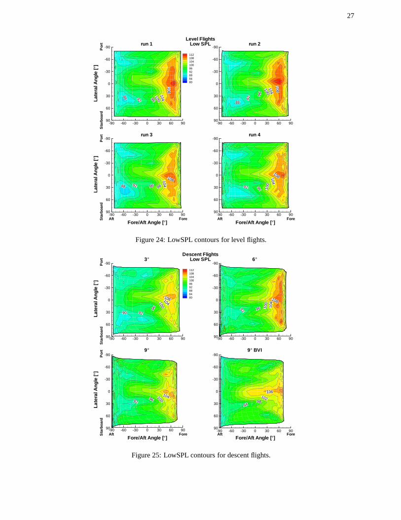
27

108

1041009692

88

-90 -60 -30 0 30 60 90

-90

-60

-30

0

30

60

90

1121081041009692888480

108104

100

96

92

88

-90 -60 -30 0 30 60 90

-90

-60

-30

0

30

60

90

108104

98969288

-90 -60 -30 0 30 60 90

-90

-60

-30

0

30

60

90

108104

1009692

-90 -60 -30 0 30 60 90

-90

-60

-30

0

30

60

90

Lat

eral

An

gle

[°]

Late

ralA

ngle

[°]

Fore/Aft Angle [°] Fore/Aft Angle [°]

Po

rtS

tarb

oar

dP

ort

Sta

rbo

ard

Aft Fore Aft Fore

Level FlightsLow SPLrun 1 run 2

run 3 run 4

Figure 24: LowSPL contours for level flights.

106104100

96

9290

-90 -60 -30 0 30 60 90

-90

-60

-30

0

30

60

90

1121081041009692888480 108

104

100

9692

-90 -60 -30 0 30 60 90

-90

-60

-30

0

30

60

90

1041009692

-90 -60 -30 0 30 60 90

-90

-60

-30

0

30

60

90

106102

9894

-90 -60 -30 0 30 60 90

-90

-60

-30

0

30

60

90

Late

ralA

ngle

[°]

Lat

eral

Ang

le[°

]

Fore/Aft Angle [°] Fore/Aft Angle [°]

Po

rtS

tarb

oar

dP

ort

Sta

rbo

ard

Aft Fore Aft Fore

Descent FlightsLow SPL3° 6°

9° 9° BVI

Figure 25: LowSPL contours for descent flights.

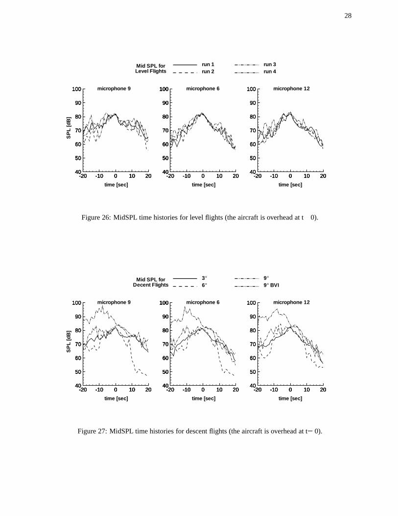
28

-20 -10 0 10 2040

50

60

70

80

90

100

-20 -10 0 10 2040

50

60

70

80

90

100

-20 -10 0 10 2040

50

60

70

80

90

100

-20 -10 0 10 2040

50

60

70

80

90

100

-20 -10 0 10 2040

50

60

70

80

90

100

-20 -10 0 10 2040

50

60

70

80

90

100

-20 -10 0 10 2040

50

60

70

80

90

100

-20 -10 0 10 2040

50

60

70

80

90

100

-20 -10 0 10 2040

50

60

70

80

90

100

-20 -10 0 10 2040

50

60

70

80

90

100

-20 -10 0 10 2040

50

60

70

80

90

100

-20 -10 0 10 2040

50

60

70

80

90

100

time [sec] time [sec] time [sec]

SP

L[d

B]

microphone 9 microphone 6 microphone 12

Mid SPL forLevel Flights

run 1run 2

run 3run 4

Figure 26: MidSPL time histories for level flights (the aircraft is overhead at t= 0).

-20 -10 0 10 2040

50

60

70

80

90

100

-20 -10 0 10 2040

50

60

70

80

90

100

-20 -10 0 10 2040

50

60

70

80

90

100

-20 -10 0 10 2040

50

60

70

80

90

100

-20 -10 0 10 2040

50

60

70

80

90

100

-20 -10 0 10 2040

50

60

70

80

90

100

-20 -10 0 10 2040

50

60

70

80

90

100

-20 -10 0 10 2040

50

60

70

80

90

100

-20 -10 0 10 2040

50

60

70

80

90

100

-20 -10 0 10 2040

50

60

70

80

90

100

-20 -10 0 10 2040

50

60

70

80

90

100

-20 -10 0 10 2040

50

60

70

80

90

100

time [sec] time [sec] time [sec]

SP

L[d

B]

microphone 9 microphone 6 microphone 12

Mid SPL forDecent Flights

3°6°

9°9° BVI

Figure 27: MidSPL time histories for descent flights (the aircraft is overhead at t= 0).

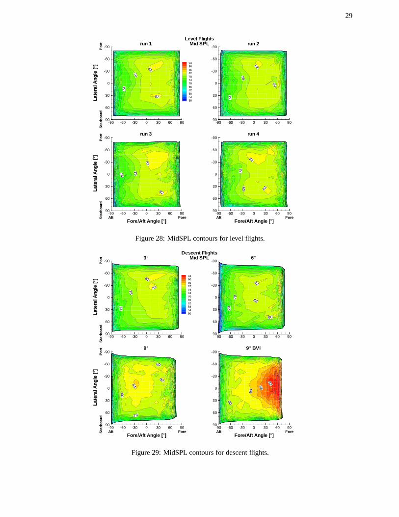
29

82

78

74

82

-90 -60 -30 0 30 60 90

-90

-60

-30

0

30

60

90

949086827874706662585450

82

78

74

80-90 -60 -30 0 30 60 90

-90

-60

-30

0

30

60

90

82

7874

82

-90 -60 -30 0 30 60 90

-90

-60

-30

0

30

60

90

82

78

82

80

-90 -60 -30 0 30 60 90

-90

-60

-30

0

30

60

90

Lat

eral

An

gle

[°]

Late

ralA

ngle

[°]

Fore/Aft Angle [°] Fore/Aft Angle [°]

Po

rtS

tarb

oar

dP

ort

Sta

rbo

ard

Aft Fore Aft Fore

Level FlightsMid SPLrun 1 run 2

run 3 run 4

Figure 28: MidSPL contours for level flights.

82

78

74

82

-90 -60 -30 0 30 60 90

-90

-60

-30

0

30

60

90

949086827874706662585450

82

78

74

82

80

-90 -60 -30 0 30 60 90

-90

-60

-30

0

30

60

90

84

80

82

80

78

-90 -60 -30 0 30 60 90

-90

-60

-30

0

30

60

90

9288

84

80

-90 -60 -30 0 30 60 90

-90

-60

-30

0

30

60

90

Late

ralA

ngle

[°]

Lat

eral

Ang

le[°

]

Fore/Aft Angle [°] Fore/Aft Angle [°]

Po

rtS

tarb

oar

dP

ort

Sta

rbo

ard

Aft Fore Aft Fore

Descent FlightsMid SPL3° 6°

9° 9° BVI

Figure 29: MidSPL contours for descent flights.

30

0 0.025 0.05 0.075 0.1-50

-40

-30

-20

-10

0

10

20

0 0.025 0.05 0.075 0.1-50

-40

-30

-20

-10

0

10

20

0 0.025 0.05 0.075 0.1-50

-40

-30

-20

-10

0

10

20

0 0.025 0.05 0.075 0.1-10

-5

0

5

10

0 0.025 0.05 0.075 0.1-10

-5

0

5

10

0 0.025 0.05 0.075 0.1-50

-40

-30

-20

-10

0

10

20

0 0.025 0.05 0.075 0.1-50

-40

-30

-20

-10

0

10

20

0 0.025 0.05 0.075 0.1-50

-40

-30

-20

-10

0

10

20

0 0.025 0.05 0.075 0.1-10

-5

0

5

10

0 0.025 0.05 0.075 0.1-10

-5

0

5

10

time [sec]

Aco

ustic

Pre

ssur

e[P

a]

15 sec prior 10 sec prior 5 sec prior overhead 5 sec after

mic 6&12

mic 9

Figure 30: Prediction One acoustic pressure time histories (normalized) for centerline and sideline micro-phones for level flight conditions, time is relative to the aircraft overhead of the microphone array.

0 0.025 0.05 0.075 0.1-50

-40

-30

-20

-10

0

10

20

0 0.025 0.05 0.075 0.1-50

-40

-30

-20

-10

0

10

20

0 0.025 0.05 0.075 0.1-50

-40

-30

-20

-10

0

10

20

0 0.025 0.05 0.075 0.1-10

-5

0

5

10

0 0.025 0.05 0.075 0.1-10

-5

0

5

10

0 0.025 0.05 0.075 0.1-50

-40

-30

-20

-10

0

10

20

0 0.025 0.05 0.075 0.1-50

-40

-30

-20

-10

0

10

20

0 0.025 0.05 0.075 0.1-50

-40

-30

-20

-10

0

10

20

0 0.025 0.05 0.075 0.1-10

-5

0

5

10

0 0.025 0.05 0.075 0.1-10

-5

0

5

10

time [sec]

Aco

ustic

Pre

ssur

e[P

a]

15 sec prior 10 sec prior 5 sec prior overhead 5 sec after

mic 6&12

mic 9

Figure 31: Prediction One acoustic pressure time histories (normalized) for centerline and sideline micro-phones for 3˚ descent condition, time is relative to the aircraft overhead of the microphone array.

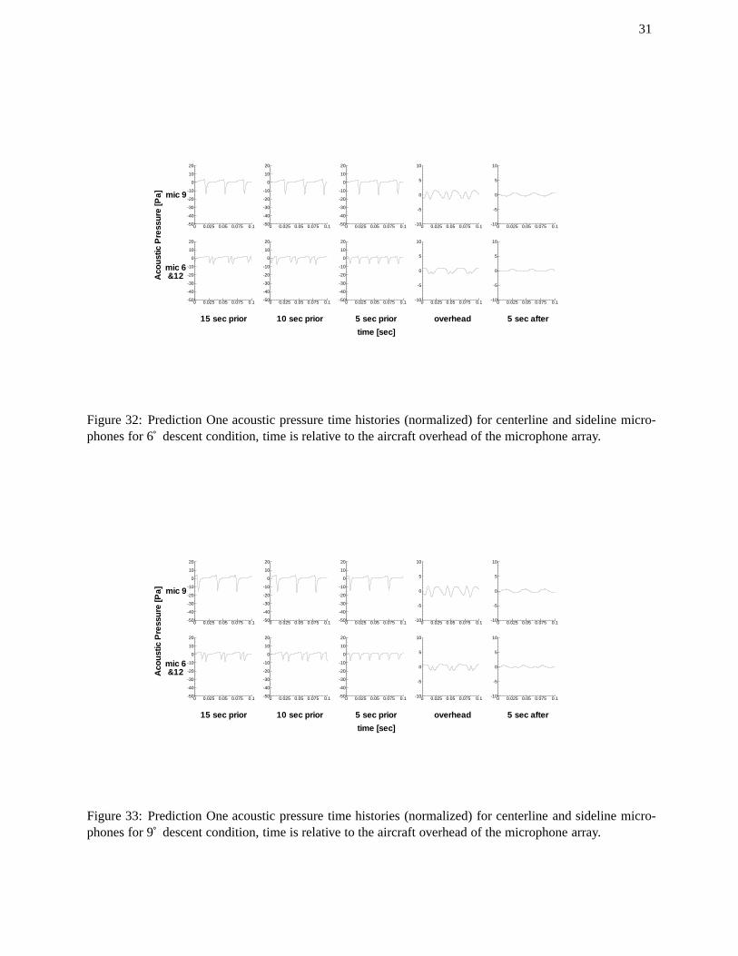
31

0 0.025 0.05 0.075 0.1-50

-40

-30

-20

-10

0

10

20

0 0.025 0.05 0.075 0.1-50

-40

-30

-20

-10

0

10

20

0 0.025 0.05 0.075 0.1-50

-40

-30

-20

-10

0

10

20

0 0.025 0.05 0.075 0.1-10

-5

0

5

10

0 0.025 0.05 0.075 0.1-10

-5

0

5

10

0 0.025 0.05 0.075 0.1-50

-40

-30

-20

-10

0

10

20

0 0.025 0.05 0.075 0.1-50

-40

-30

-20

-10

0

10

20

0 0.025 0.05 0.075 0.1-50

-40

-30

-20

-10

0

10

20

0 0.025 0.05 0.075 0.1-10

-5

0

5

10

0 0.025 0.05 0.075 0.1-10

-5

0

5

10

time [sec]

Aco

ustic

Pre

ssur

e[P

a]

15 sec prior 10 sec prior 5 sec prior overhead 5 sec after

mic 6&12

mic 9

Figure 32: Prediction One acoustic pressure time histories (normalized) for centerline and sideline micro-phones for 6˚ descent condition, time is relative to the aircraft overhead of the microphone array.

0 0.025 0.05 0.075 0.1-50

-40

-30

-20

-10

0

10

20

0 0.025 0.05 0.075 0.1-50

-40

-30

-20

-10

0

10

20

0 0.025 0.05 0.075 0.1-50

-40

-30

-20

-10

0

10

20

0 0.025 0.05 0.075 0.1-10

-5

0

5

10

0 0.025 0.05 0.075 0.1-10

-5

0

5

10

0 0.025 0.05 0.075 0.1-50

-40

-30

-20

-10

0

10

20

0 0.025 0.05 0.075 0.1-50

-40

-30

-20

-10

0

10

20

0 0.025 0.05 0.075 0.1-50

-40

-30

-20

-10

0

10

20

0 0.025 0.05 0.075 0.1-10

-5

0

5

10

0 0.025 0.05 0.075 0.1-10

-5

0

5

10

time [sec]

Aco

ustic

Pre

ssur

e[P

a]

15 sec prior 10 sec prior 5 sec prior overhead 5 sec after

mic 6&12

mic 9

Figure 33: Prediction One acoustic pressure time histories (normalized) for centerline and sideline micro-phones for 9˚ descent condition, time is relative to the aircraft overhead of the microphone array.

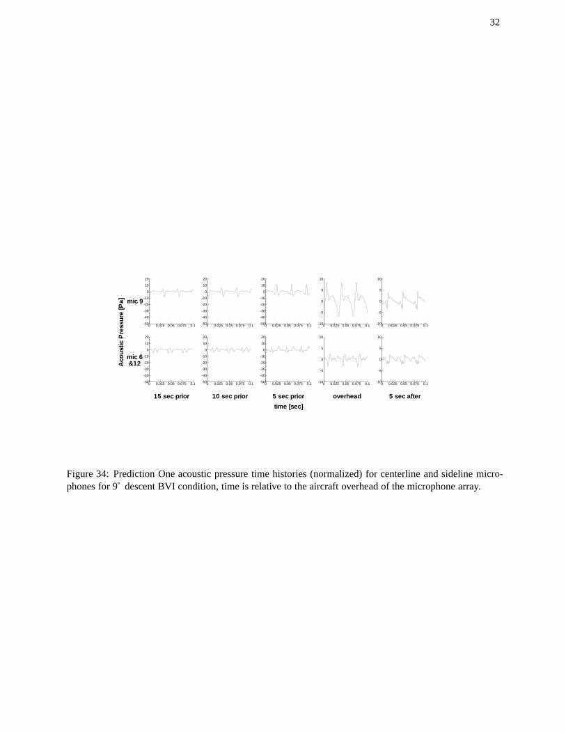
32

0 0.025 0.05 0.075 0.1-50

-40

-30

-20

-10

0

10

20

0 0.025 0.05 0.075 0.1-50

-40

-30

-20

-10

0

10

20

0 0.025 0.05 0.075 0.1-50

-40

-30

-20

-10

0

10

20

0 0.025 0.05 0.075 0.1-10

-5

0

5

10

0 0.025 0.05 0.075 0.1-10

-5

0

5

10

0 0.025 0.05 0.075 0.1-50

-40

-30

-20

-10

0

10

20

0 0.025 0.05 0.075 0.1-50

-40

-30

-20

-10

0

10

20

0 0.025 0.05 0.075 0.1-50

-40

-30

-20

-10

0

10

20

0 0.025 0.05 0.075 0.1-10

-5

0

5

10

0 0.025 0.05 0.075 0.1-10

-5

0

5

10

time [sec]

Aco

ustic

Pre

ssur

e[P

a]

15 sec prior 10 sec prior 5 sec prior overhead 5 sec after

mic 6&12

mic 9

Figure 34: Prediction One acoustic pressure time histories (normalized) for centerline and sideline micro-phones for 9˚ descent BVI condition, time is relative to the aircraft overhead of the microphone array.

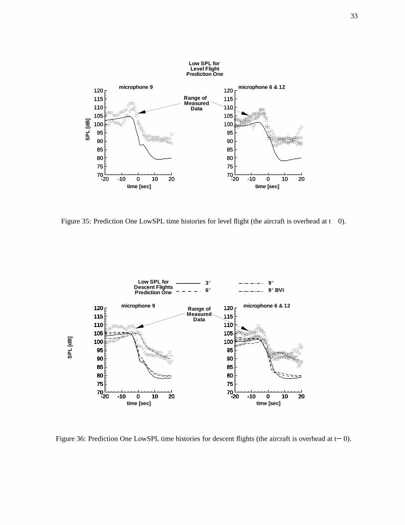
33

-20 -10 0 10 2070

75

80

85

90

95

100

105

110

115

120

-20 -10 0 10 2070

75

80

85

90

95

100

105

110

115

120

-20 -10 0 10 2070

75

80

85

90

95

100

105

110

115

120

-20 -10 0 10 2070

75

80

85

90

95

100

105

110

115

120

time [sec] time [sec]

SP

L[d

B]

microphone 9 microphone 6 & 12

Low SPL forLevel Flight

Prediction One

Range ofMeasured

Data

Figure 35: Prediction One LowSPL time histories for level flight (the aircraft is overhead at t= 0).

-20 -10 0 10 2070

75

80

85

90

95

100

105

110

115

120

-20 -10 0 10 2070

75

80

85

90

95

100

105

110

115

120

-20 -10 0 10 2070

75

80

85

90

95

100

105

110

115

120

-20 -10 0 10 2070

75

80

85

90

95

100

105

110

115

120

-20 -10 0 10 2070

75

80

85

90

95

100

105

110

115

120

-20 -10 0 10 2070

75

80

85

90

95

100

105

110

115

120

-20 -10 0 10 2070

75

80

85

90

95

100

105

110

115

120

-20 -10 0 10 2070

75

80

85

90

95

100

105

110

115

120

-20 -10 0 10 2070

75

80

85

90

95

100

105

110

115

120

-20 -10 0 10 2070

75

80

85

90

95

100

105

110

115

120

time [sec] time [sec]

SP

L[d

B]

microphone 9 microphone 6 & 12

Low SPL forDescent FlightsPrediction One

3°6°

9°9° BVI

Range ofMeasured

Data

Figure 36: Prediction One LowSPL time histories for descent flights (the aircraft is overhead at t= 0).

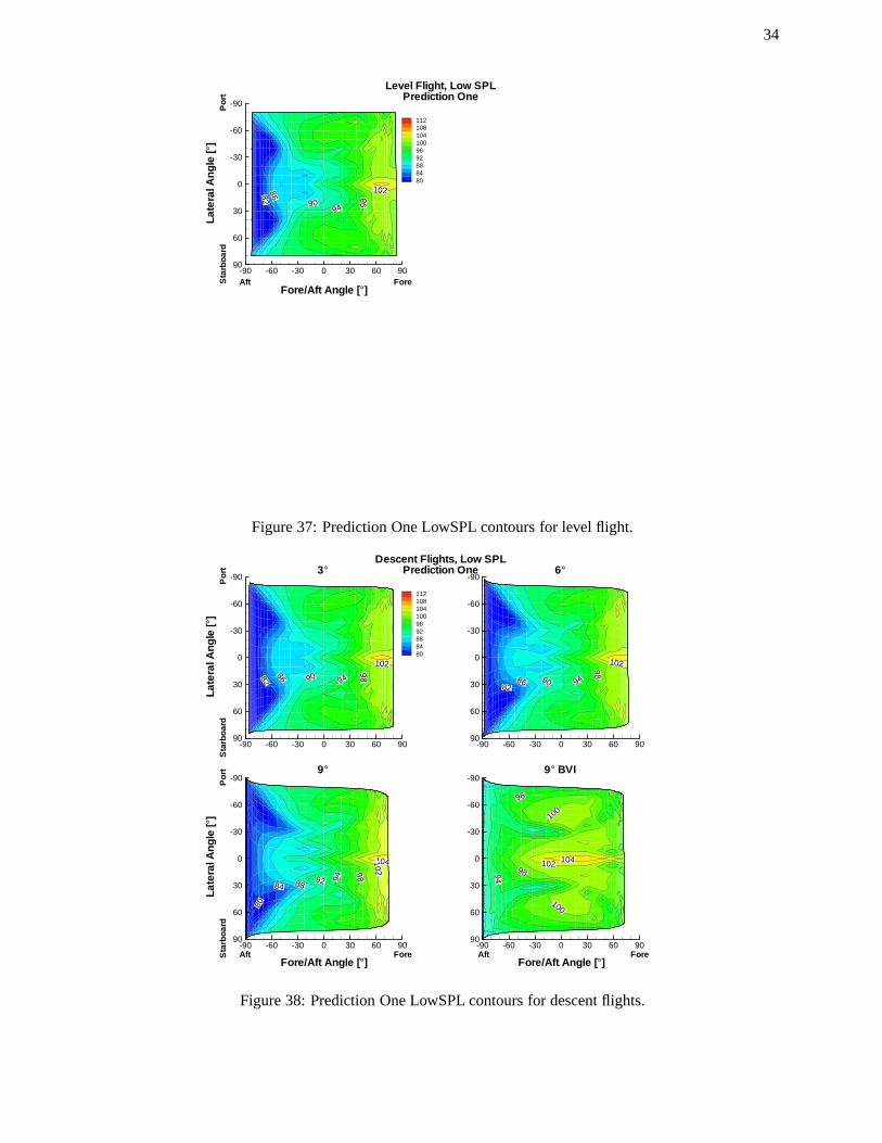
34

102

98

9490

8682

-90 -60 -30 0 30 60 90

-90

-60

-30

0

30

60

90

1121081041009692888480

Lat

eral

An

gle

[°]

Fore/Aft Angle [°]

Po

rtS

tarb

oar

d

Aft Fore

Level Flight, Low SPLPrediction One

Figure 37: Prediction One LowSPL contours for level flight.

102

98

94908682

-90 -60 -30 0 30 60 90

-90

-60

-30

0

30

60

90

1121081041009692888480

10298

94908682

-90 -60 -30 0 30 60 90

-90

-60

-30

0

30

60

90

1041029894928884

80

-90 -60 -30 0 30 60 90

-90

-60

-30

0

30

60

90

1041029894

100

96

100

-90 -60 -30 0 30 60 90

-90

-60

-30

0

30

60

90

Late

ralA

ngle

[°]

Lat

eral

Ang

le[°

]

Fore/Aft Angle [°] Fore/Aft Angle [°]

Po

rtS

tarb

oar

dP

ort

Sta

rbo

ard

Aft Fore Aft Fore

Descent Flights, Low SPLPrediction One3° 6°

9° 9° BVI

Figure 38: Prediction One LowSPL contours for descent flights.

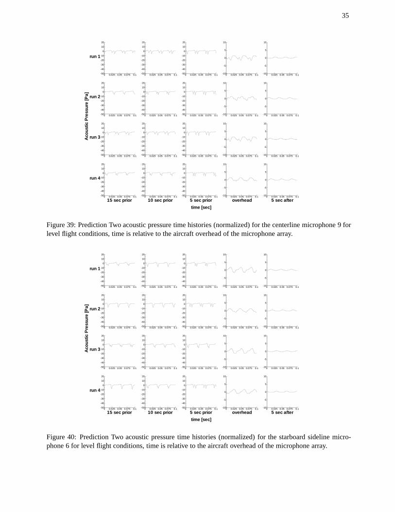
35

0 0.025 0.05 0.075 0.1-50

-40

-30

-20

-10

0

10

20

0 0.025 0.05 0.075 0.1-50

-40

-30

-20

-10

0

10

20

0 0.025 0.05 0.075 0.1-50

-40

-30

-20

-10

0

10

20

0 0.025 0.05 0.075 0.1-10

-5

0

5

10

0 0.025 0.05 0.075 0.1-10

-5

0

5

10

0 0.025 0.05 0.075 0.1-50

-40

-30

-20

-10

0

10

20

0 0.025 0.05 0.075 0.1-50

-40

-30

-20

-10

0

10

20

0 0.025 0.05 0.075 0.1-50

-40

-30

-20

-10

0

10

20

0 0.025 0.05 0.075 0.1-10

-5

0

5

10

0 0.025 0.05 0.075 0.1-10

-5

0

5

10

0 0.025 0.05 0.075 0.1-50

-40

-30

-20

-10

0

10

20

0 0.025 0.05 0.075 0.1-50

-40

-30

-20

-10

0

10

20

0 0.025 0.05 0.075 0.1-50

-40

-30

-20

-10

0

10

20

0 0.025 0.05 0.075 0.1-10

-5

0

5

10

0 0.025 0.05 0.075 0.1-10

-5

0

5

10

0 0.025 0.05 0.075 0.1-50

-40

-30

-20

-10

0

10

20

0 0.025 0.05 0.075 0.1-50

-40

-30

-20

-10

0

10

20

0 0.025 0.05 0.075 0.1-50

-40

-30

-20

-10

0

10

20

0 0.025 0.05 0.075 0.1-10

-5

0

5

10

0 0.025 0.05 0.075 0.1-10

-5

0

5

10

time [sec]

Aco

ustic

Pre

ssur

e[P

a]

15 sec prior 10 sec prior 5 sec prior overhead 5 sec after

run 4

run 3

run 2

run 1

Figure 39: Prediction Two acoustic pressure time histories (normalized) for the centerline microphone 9 forlevel flight conditions, time is relative to the aircraft overhead of the microphone array.

0 0.025 0.05 0.075 0.1-50

-40

-30

-20

-10

0

10

20

0 0.025 0.05 0.075 0.1-50

-40

-30

-20

-10

0

10

20

0 0.025 0.05 0.075 0.1-50

-40

-30

-20

-10

0

10

20

0 0.025 0.05 0.075 0.1-10

-5

0

5

10

0 0.025 0.05 0.075 0.1-10

-5

0

5

10

0 0.025 0.05 0.075 0.1-50

-40

-30

-20

-10

0

10

20

0 0.025 0.05 0.075 0.1-50

-40

-30

-20

-10

0

10

20

0 0.025 0.05 0.075 0.1-50

-40

-30

-20

-10

0

10

20

0 0.025 0.05 0.075 0.1-10

-5

0

5

10

0 0.025 0.05 0.075 0.1-10

-5

0

5

10

0 0.025 0.05 0.075 0.1-50

-40

-30

-20

-10

0

10

20

0 0.025 0.05 0.075 0.1-50

-40

-30

-20

-10

0

10

20

0 0.025 0.05 0.075 0.1-50

-40

-30

-20

-10

0

10

20

0 0.025 0.05 0.075 0.1-10

-5

0

5

10

0 0.025 0.05 0.075 0.1-10

-5

0

5

10

0 0.025 0.05 0.075 0.1-50

-40

-30

-20

-10

0

10

20

0 0.025 0.05 0.075 0.1-50

-40

-30

-20

-10

0

10

20

0 0.025 0.05 0.075 0.1-50

-40

-30

-20

-10

0

10

20

0 0.025 0.05 0.075 0.1-10

-5

0

5

10

0 0.025 0.05 0.075 0.1-10

-5

0

5

10

time [sec]

Aco

ustic

Pre

ssur

e[P

a]

15 sec prior 10 sec prior 5 sec prior overhead 5 sec after

run 4

run 3

run 2

run 1

Figure 40: Prediction Two acoustic pressure time histories (normalized) for the starboard sideline micro-phone 6 for level flight conditions, time is relative to the aircraft overhead of the microphone array.

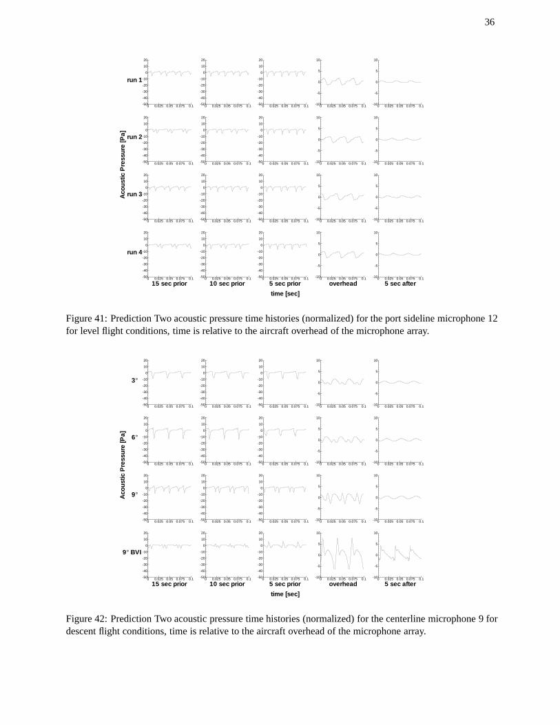
36

0 0.025 0.05 0.075 0.1-50

-40

-30

-20

-10

0

10

20

0 0.025 0.05 0.075 0.1-50

-40

-30

-20

-10

0

10

20

0 0.025 0.05 0.075 0.1-50

-40

-30

-20

-10

0

10

20

0 0.025 0.05 0.075 0.1-10

-5

0

5

10

0 0.025 0.05 0.075 0.1-10

-5

0

5

10

0 0.025 0.05 0.075 0.1-50

-40

-30

-20

-10

0

10

20

0 0.025 0.05 0.075 0.1-50

-40

-30

-20

-10

0

10

20

0 0.025 0.05 0.075 0.1-50

-40

-30

-20

-10

0

10

20

0 0.025 0.05 0.075 0.1-10

-5

0

5

10

0 0.025 0.05 0.075 0.1-10

-5

0

5

10

0 0.025 0.05 0.075 0.1-50

-40

-30

-20

-10

0

10

20

0 0.025 0.05 0.075 0.1-50

-40

-30

-20

-10

0

10

20

0 0.025 0.05 0.075 0.1-50

-40

-30

-20

-10

0

10

20

0 0.025 0.05 0.075 0.1-10

-5

0

5

10

0 0.025 0.05 0.075 0.1-10

-5

0

5

10

0 0.025 0.05 0.075 0.1-50

-40

-30

-20

-10

0

10

20

0 0.025 0.05 0.075 0.1-50

-40

-30

-20

-10

0

10

20

0 0.025 0.05 0.075 0.1-50

-40

-30

-20

-10

0

10

20

0 0.025 0.05 0.075 0.1-10

-5

0

5

10

0 0.025 0.05 0.075 0.1-10

-5

0

5

10

time [sec]

Aco

ustic

Pre

ssur

e[P

a]

15 sec prior 10 sec prior 5 sec prior overhead 5 sec after

run 4

run 3

run 2

run 1

Figure 41: Prediction Two acoustic pressure time histories (normalized) for the port sideline microphone 12for level flight conditions, time is relative to the aircraft overhead of the microphone array.

0 0.025 0.05 0.075 0.1-50

-40

-30

-20

-10

0

10

20

0 0.025 0.05 0.075 0.1-50

-40

-30

-20

-10

0

10

20

0 0.025 0.05 0.075 0.1-50

-40

-30

-20

-10

0

10

20

0 0.025 0.05 0.075 0.1-10

-5

0

5

10

0 0.025 0.05 0.075 0.1-10

-5

0

5

10

0 0.025 0.05 0.075 0.1-50

-40

-30

-20

-10

0

10

20

0 0.025 0.05 0.075 0.1-50

-40

-30

-20

-10

0

10

20

0 0.025 0.05 0.075 0.1-50

-40

-30

-20

-10

0

10

20

0 0.025 0.05 0.075 0.1-10

-5

0

5

10

0 0.025 0.05 0.075 0.1-10

-5

0

5

10

0 0.025 0.05 0.075 0.1-50

-40

-30

-20

-10

0

10

20

0 0.025 0.05 0.075 0.1-50

-40

-30

-20

-10

0

10

20

0 0.025 0.05 0.075 0.1-50

-40

-30

-20

-10

0

10

20

0 0.025 0.05 0.075 0.1-10

-5

0

5

10

0 0.025 0.05 0.075 0.1-10

-5

0

5

10

0 0.025 0.05 0.075 0.1-50

-40

-30

-20

-10

0

10

20

0 0.025 0.05 0.075 0.1-50

-40

-30

-20

-10

0

10

20

0 0.025 0.05 0.075 0.1-50

-40

-30

-20

-10

0

10

20

0 0.025 0.05 0.075 0.1-10

-5

0

5

10

0 0.025 0.05 0.075 0.1-10

-5

0

5

10

time [sec]

Aco

ustic

Pre

ssur

e[P

a]

15 sec prior 10 sec prior 5 sec prior overhead 5 sec after

9° BVI

9°

6°

3°

Figure 42: Prediction Two acoustic pressure time histories (normalized) for the centerline microphone 9 fordescent flight conditions, time is relative to the aircraft overhead of the microphone array.

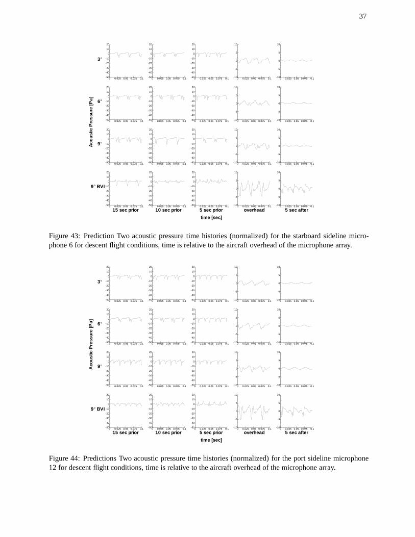
37

0 0.025 0.05 0.075 0.1-50

-40

-30

-20

-10

0

10

20

0 0.025 0.05 0.075 0.1-50

-40

-30

-20

-10

0

10

20

0 0.025 0.05 0.075 0.1-50

-40

-30

-20

-10

0

10

20

0 0.025 0.05 0.075 0.1-10

-5

0

5

10

0 0.025 0.05 0.075 0.1-10

-5

0

5

10

0 0.025 0.05 0.075 0.1-50

-40

-30

-20

-10

0

10

20

0 0.025 0.05 0.075 0.1-50

-40

-30

-20

-10

0

10

20

0 0.025 0.05 0.075 0.1-50

-40

-30

-20

-10

0

10

20

0 0.025 0.05 0.075 0.1-10

-5

0

5

10

0 0.025 0.05 0.075 0.1-10

-5

0

5

10

0 0.025 0.05 0.075 0.1-50

-40

-30

-20

-10

0

10

20

0 0.025 0.05 0.075 0.1-50

-40

-30

-20

-10

0

10

20

0 0.025 0.05 0.075 0.1-50

-40

-30

-20

-10

0

10

20

0 0.025 0.05 0.075 0.1-10

-5

0

5

10

0 0.025 0.05 0.075 0.1-10

-5

0

5

10

0 0.025 0.05 0.075 0.1-50

-40

-30

-20

-10

0

10

20

0 0.025 0.05 0.075 0.1-50

-40

-30

-20

-10

0

10

20

0 0.025 0.05 0.075 0.1-50

-40

-30

-20

-10

0

10

20

0 0.025 0.05 0.075 0.1-10

-5

0

5

10

0 0.025 0.05 0.075 0.1-10

-5

0

5

10

time [sec]

Aco

ustic

Pre

ssur

e[P

a]

15 sec prior 10 sec prior 5 sec prior overhead 5 sec after

9° BVI

9°

6°

3°

Figure 43: Prediction Two acoustic pressure time histories (normalized) for the starboard sideline micro-phone 6 for descent flight conditions, time is relative to the aircraft overhead of the microphone array.

0 0.025 0.05 0.075 0.1-50

-40

-30

-20

-10

0

10

20

0 0.025 0.05 0.075 0.1-50

-40

-30

-20

-10

0

10

20

0 0.025 0.05 0.075 0.1-50

-40

-30

-20

-10

0

10

20

0 0.025 0.05 0.075 0.1-10

-5

0

5

10

0 0.025 0.05 0.075 0.1-10

-5

0

5

10

0 0.025 0.05 0.075 0.1-50

-40

-30

-20

-10

0

10

20

0 0.025 0.05 0.075 0.1-50

-40

-30

-20

-10

0

10

20

0 0.025 0.05 0.075 0.1-50

-40

-30

-20

-10

0

10

20

0 0.025 0.05 0.075 0.1-10

-5

0

5

10

0 0.025 0.05 0.075 0.1-10

-5

0

5

10

0 0.025 0.05 0.075 0.1-50

-40

-30

-20

-10

0

10

20

0 0.025 0.05 0.075 0.1-50

-40

-30

-20

-10

0

10

20

0 0.025 0.05 0.075 0.1-50

-40

-30

-20

-10

0

10

20

0 0.025 0.05 0.075 0.1-10

-5

0

5

10

0 0.025 0.05 0.075 0.1-10

-5

0

5

10

0 0.025 0.05 0.075 0.1-50

-40

-30

-20

-10

0

10

20

0 0.025 0.05 0.075 0.1-50

-40

-30

-20

-10

0

10

20

0 0.025 0.05 0.075 0.1-50

-40

-30

-20

-10

0

10

20

0 0.025 0.05 0.075 0.1-10

-5

0

5

10

0 0.025 0.05 0.075 0.1-10

-5

0

5

10

time [sec]

Aco

ustic

Pre

ssur

e[P

a]

15 sec prior 10 sec prior 5 sec prior overhead 5 sec after

9° BVI

9°

6°

3°

Figure 44: Predictions Two acoustic pressure time histories (normalized) for the port sideline microphone12 for descent flight conditions, time is relative to the aircraft overhead of the microphone array.

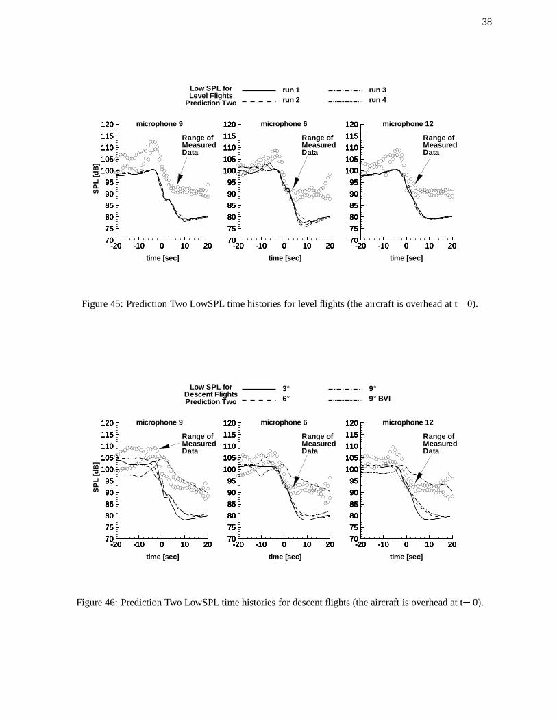
38

-20 -10 0 10 2070

75

80

85

90

95

100

105

110

115

120

-20 -10 0 10 2070

75

80

85

90

95

100

105

110

115

120

-20 -10 0 10 2070

75

80

85

90

95

100

105

110

115

120

-20 -10 0 10 2070

75

80

85

90

95

100

105

110

115

120

-20 -10 0 10 2070

75

80

85

90

95

100

105

110

115

120

-20 -10 0 10 2070

75

80

85

90

95

100

105

110

115

120

-20 -10 0 10 2070

75

80

85

90

95

100

105

110

115

120

-20 -10 0 10 2070

75

80

85

90

95

100

105

110

115

120

-20 -10 0 10 2070

75

80

85

90

95

100

105

110

115

120

-20 -10 0 10 2070

75

80

85

90

95

100

105

110

115

120

-20 -10 0 10 2070

75

80

85

90

95

100

105

110

115

120

-20 -10 0 10 2070

75

80

85

90

95

100

105

110

115

120

-20 -10 0 10 2070

75

80

85

90

95

100

105

110

115

120

-20 -10 0 10 2070

75

80

85

90

95

100

105

110

115

120

-20 -10 0 10 2070

75

80

85

90

95

100

105

110

115

120

time [sec] time [sec] time [sec]

SP

L[d

B]

microphone 9 microphone 6 microphone 12

Low SPL forLevel Flights

Prediction Two

run 1run 2

run 3run 4

Range ofMeasuredData

Range ofMeasuredData

Range ofMeasuredData

Figure 45: Prediction Two LowSPL time histories for level flights (the aircraft is overhead at t= 0).

-20 -10 0 10 2070

75

80

85

90

95

100

105

110

115

120

-20 -10 0 10 2070

75

80

85

90

95

100

105

110

115

120

-20 -10 0 10 2070

75

80

85

90

95

100

105

110

115

120

-20 -10 0 10 2070

75

80

85

90

95

100

105

110

115

120

-20 -10 0 10 2070

75

80

85

90

95

100

105

110

115

120

-20 -10 0 10 2070

75

80

85

90

95

100

105

110

115

120

-20 -10 0 10 2070

75

80

85

90

95

100

105

110

115

120

-20 -10 0 10 2070

75

80

85

90

95

100

105

110

115

120

-20 -10 0 10 2070

75

80

85

90

95

100

105

110

115

120

-20 -10 0 10 2070

75

80

85

90

95

100

105

110

115

120

-20 -10 0 10 2070

75

80

85

90

95

100

105

110

115

120

-20 -10 0 10 2070

75

80

85

90

95

100

105

110

115

120

-20 -10 0 10 2070

75

80

85

90

95

100

105

110

115

120

-20 -10 0 10 2070

75

80

85

90

95

100

105

110

115

120

-20 -10 0 10 2070

75

80

85

90

95

100

105

110

115

120

time [sec] time [sec] time [sec]

SP

L[d

B]

microphone 9 microphone 6 microphone 12

Low SPL forDescent FlightsPrediction Two

3°6°

9°9° BVI

Range ofMeasuredData

Range ofMeasuredData

Range ofMeasuredData

Figure 46: Prediction Two LowSPL time histories for descent flights (the aircraft is overhead at t= 0).

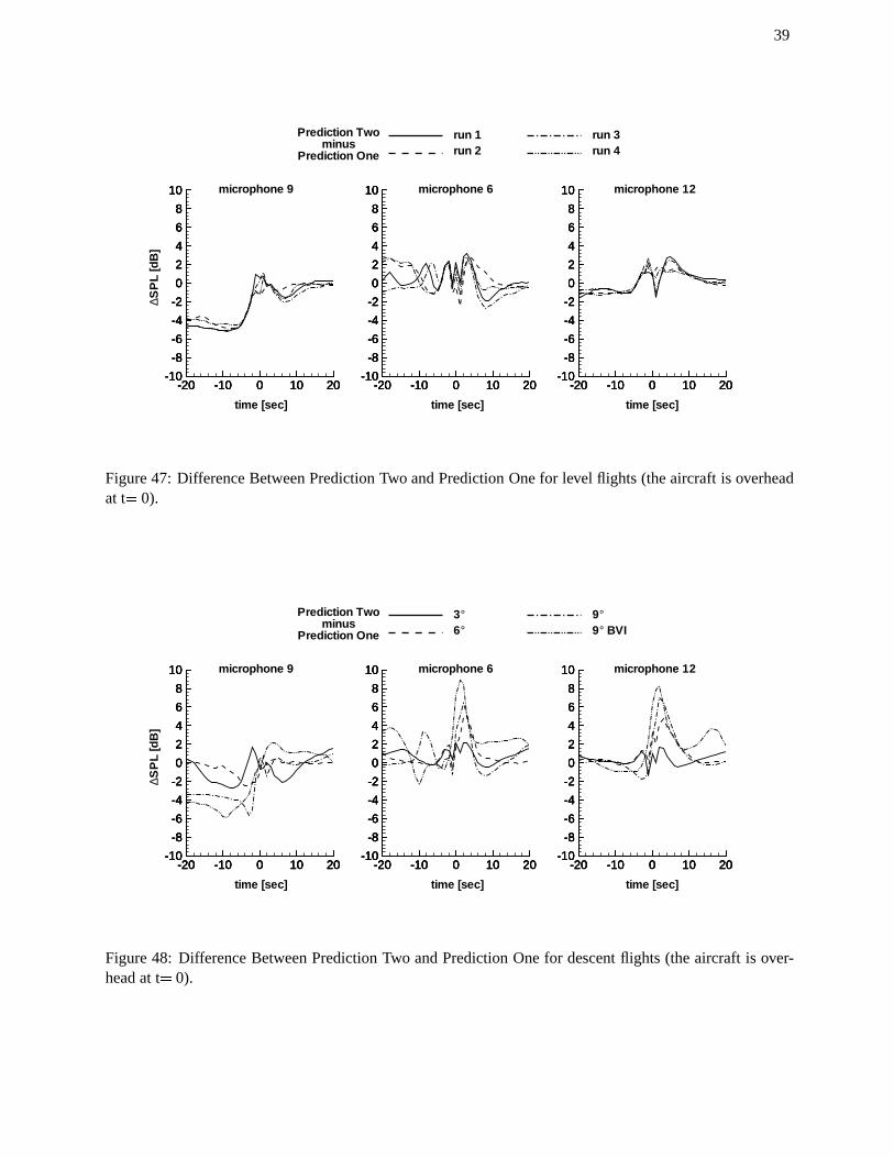
39

-20 -10 0 10 20-10

-8

-6

-4

-2

0

2

4

6

8

10

-20 -10 0 10 20-10

-8

-6

-4

-2

0

2

4

6

8

10

-20 -10 0 10 20-10

-8

-6

-4

-2

0

2

4

6

8

10

-20 -10 0 10 20-10

-8

-6

-4

-2

0

2

4

6

8

10

-20 -10 0 10 20-10

-8

-6

-4

-2

0

2

4

6

8

10

-20 -10 0 10 20-10

-8

-6

-4

-2

0

2

4

6

8

10

-20 -10 0 10 20-10

-8

-6

-4

-2

0

2

4

6

8

10

-20 -10 0 10 20-10

-8

-6

-4

-2

0

2

4

6

8

10

-20 -10 0 10 20-10

-8

-6

-4

-2

0

2

4

6

8

10

-20 -10 0 10 20-10

-8

-6

-4

-2

0

2

4

6

8

10

-20 -10 0 10 20-10

-8

-6

-4

-2

0

2

4

6

8

10

-20 -10 0 10 20-10

-8

-6

-4

-2

0

2

4

6

8

10

time [sec] time [sec] time [sec]

∆SP

L[d

B]

microphone 9 microphone 6 microphone 12

Prediction Twominus

Prediction One

run 1run 2

run 3run 4

Figure 47: Difference Between Prediction Two and Prediction One for level flights (the aircraft is overheadat t= 0).

-20 -10 0 10 20-10

-8

-6

-4

-2

0

2

4

6

8

10

-20 -10 0 10 20-10

-8

-6

-4

-2

0

2

4

6

8

10

-20 -10 0 10 20-10

-8

-6

-4

-2

0

2

4

6

8

10

-20 -10 0 10 20-10

-8

-6

-4

-2

0

2

4

6

8

10

-20 -10 0 10 20-10

-8

-6

-4

-2

0

2

4

6

8

10

-20 -10 0 10 20-10

-8

-6

-4

-2

0

2

4

6

8

10

-20 -10 0 10 20-10

-8

-6

-4

-2

0

2

4

6

8

10

-20 -10 0 10 20-10

-8

-6

-4

-2

0

2

4

6

8

10

-20 -10 0 10 20-10

-8

-6

-4

-2

0

2

4

6

8

10

-20 -10 0 10 20-10

-8

-6

-4

-2

0

2

4

6

8

10

-20 -10 0 10 20-10

-8

-6

-4

-2

0

2

4

6

8

10

-20 -10 0 10 20-10

-8

-6

-4

-2

0

2

4

6

8

10

time [sec] time [sec] time [sec]

∆SP

L[d

B]

microphone 9 microphone 6 microphone 12

Prediction Twominus

Prediction One

3°6°

9°9° BVI

Figure 48: Difference Between Prediction Two and Prediction One for descent flights (the aircraft is over-head at t= 0).

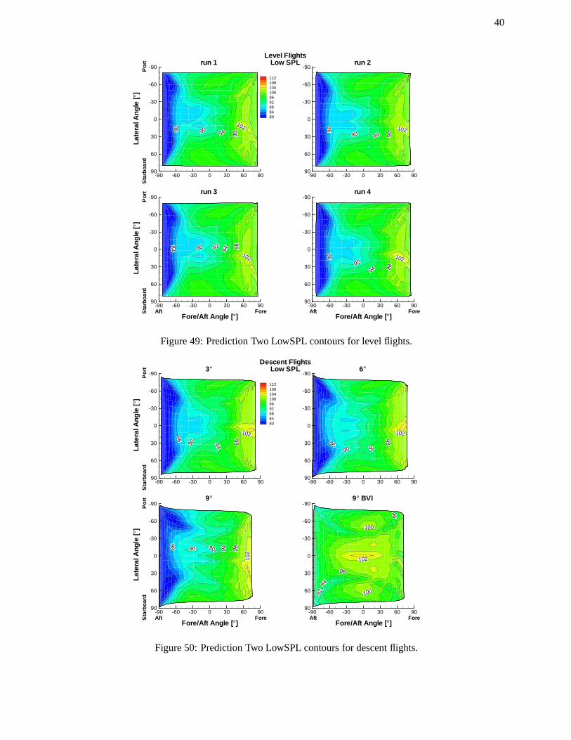
40

102

989490

86

-90 -60 -30 0 30 60 90

-90

-60

-30

0

30

60

90

1121081041009692888480

102

989490

86

-90 -60 -30 0 30 60 90

-90

-60

-30

0

30

60

90

102

98949288

84

-90 -60 -30 0 30 60 90

-90

-60

-30

0

30

60

90

102

989490

86

-90 -60 -30 0 30 60 90

-90

-60

-30

0

30

60

90

Lat

eral

An

gle

[°]

Late

ralA

ngle

[°]

Fore/Aft Angle [°] Fore/Aft Angle [°]

Po

rtS

tarb

oar

dP

ort

Sta

rbo

ard

Aft Fore Aft Fore

Level FlightsLow SPLrun 1 run 2

run 3 run 4

Figure 49: Prediction Two LowSPL contours for level flights.

102

989490

86

-90 -60 -30 0 30 60 90

-90

-60

-30

0

30

60

90

1121081041009692888480

102

98

9490

86

-90 -60 -30 0 30 60 90

-90

-60

-30

0

30

60

90

1029894909086

-90 -60 -30 0 30 60 90

-90

-60

-30

0

30

60

90

102

98

9492 100

100

96

-90 -60 -30 0 30 60 90

-90

-60

-30

0

30

60

90

Late

ralA

ngle

[°]

Lat

eral

Ang

le[°

]

Fore/Aft Angle [°] Fore/Aft Angle [°]

Po

rtS

tarb

oar

dP

ort

Sta

rbo

ard

Aft Fore Aft Fore

Descent FlightsLow SPL3° 6°

9° 9° BVI

Figure 50: Prediction Two LowSPL contours for descent flights.