TILTROTOR MODELLING FOR SIMULATION IN VARIOUS FLIGHT

JOURNAL OF THEORETICAL

AND APPLIED MECHANICS

44, 4, pp. 881-906, Warsaw 2006

TILTROTOR MODELLING FOR SIMULATION IN VARIOUS

FLIGHT CONDITIONS

Marek Miller

Institute of Aviation, Warsaw

e-mail: [email protected]

Janusz Narkiewicz

Institute of Aeronautics and Applied Mechanics, Warsaw University of Technology

e-mail: [email protected]

A computer model of a tilt-rotor has been developed for calculating perfor-mance, simulating flight and investigating stability and control. The modelis composed of a fuselage, wings, an empennage, engine nacelles and ro-tors. Tiltrotor equations of motion have been obtained by summing upinertia, gravity and aerodynamic loads acting on each part of the aircraft.Aerodynamic loads at wings, empennage and rotor blades have been cal-culated using a quasisteady model. For rotor induced velocity, the Glauertmodel has been used. The influence of the rotor inflow wing and empen-nage aerodynamic loads has been found using the actual value of inducedvelocity. The computer program of tilt-rotor model has been developed inthe MatLab environment. The sub-programs for load calculation have beensupplemented by modules for calculation of trim states and stability andcontrol matrices. During the first stage of model investigation, steady fli-ght conditions were calculated, which gave insight into rotorcraft behaviourand model quality.

Key words: tiltrotor, rotorcraft, flight control, simulation

Notations

Indicies

a – aerodynamicb – inertiac – related to three-dimensional body (fuselage, nacelle)f – fuselage

882 M. Miller, J. Narkiewicz

g,G – gravityh – horizontal stabilizeri – inertiaI = 1 – element (wing, nacelle, rotor) on right side of aircraftI = 2 – element (wing, nacelle, rotor) on left side of aircraftJ = 1, 2, 3 – rotor blade index of i-th rotorm – aerodynamic moment, moving element, massn – nacellep – aircraft, fuselager – rotor

Matrices and vectors

A – rotation matrix of moving element, A = A(φ,ϕ, γ)AG – aircraft rotation matrixAr – transformation matrix of coordinate system in airfoilAV – velocity matrixC – control vector, C = [τ, δw, δh, δv,Θ]

⊤

Ix – inertia matrix of x-th elementk() – coefficients of inflow due rotors and wings

Qxy – y-th loads of x-th element, Qxy = [F xy,Mxy]⊤

V – vector of linear velocity in Opxpypzp, V = [U, V,W ]⊤

V a – section velocityV c – vector of linear velocity of three-dimensional bodyU – induced velocity in OpxpypzpW – wind velocity in Opxpypzp∆W () – inflow due rotors and wings in OpxpypzpX – vector of aircraft motion,

X = [V ,Ω,xg,Φ]⊤ = [U, V,W,P,Q,R, xg , yg, zg, Φ,Θ, Ψ ]

⊤

Y x – state vector of x-th elementg – vector of gravity accelerationgp – vector of gravity acceleration in OpxpypzprCG – position of C.G. in OpxpypzprnCG – position of C.G. in moving element coordinate systemrn – position of moving element coordinate system in Opxpypzpxg – translation of aircraft relative to ground, xg = [xg, yg, zg]

⊤

Ω – vector of angular velocity in Opxpypzp, Ω = [P,Q,R]⊤

Ωp – velocity matrix of plane (non-moving element)Ωm – velocity matrix of moving elementΦ – Euler’s angles described as vector, Φ = [Φ,Θ, Ψ ]⊤

Θ – control of rotor swash-plates, Θ = [Θ01, Θ02, Θ11, Θ12, Θ21, Θ22]⊤

Tiltrotor modelling for simulation... 883

δw – inclination angles of wing flaps (ailerons),δw = [δw11, δw12, δw21, δw22]

⊤

δh – inclination angles of elevators, δh = [δh1, δh2, δh3]⊤

δv – inclination angles of rudders, δv = [δv1, δv2]⊤

ω – angular velocity of rotors, ω = [ω1, ω2]⊤

τ – angle of nacelle tilt

Coefficients

Ar – characteristic areaCx(α, δ) – drag coefficient (in 2D flow)Cz(α, δ) – lift coefficient (in 2D flow)Cmy(α, δ) – aerodynamic pitch moment coefficient (in 2D flow)Cxc(α, δ) – drag coefficient (in 3D flow)Cyc(α, δ) – side force coefficient (in 3D flow)Czc(α, δ) – lift coefficient (in 3D flow)Cmxc(α, δ) – aerodynamic bank moment coefficient (in 3D flow)Cmyc(α, δ) – aerodynamic pitch moment coefficient (in 3D flow)Cmzc(α, δ) – aerodynamic yaw moment coefficient (in 3D flow)Rr – characteristic lengthVa – modulus of motion velocity of section Va = |V a|c(y) – chord (characteristic dimension)g – gravity accelerationmx – mass of x-th elementα – angle of attackβ – slip angleδ – angle of inclination of steering elementρ – air density

1. Introduction

In the recent years, increasing interest in tilt rotor technology is observedamong rotorcraft community. The development of V-22 aircraft spurred a gre-at research and development effort in tilt rotor aerodynamics (McVeigh etal., 2004), acoustics (Polak and George, 1998), flight control (Weakley et al.,2003), aeroelasticity (Nixon et al., 2003), etc. The next tilt rotor project, Bell-Agusta BA 609, initiated a tilt-rotor design effort in Europe. Recently, severalEuropean research projects concerning tilt rotor technology are going on orhave already been completed (Cicale, 2003), and some new initiatives appe-ared. Despite the expanding interest in development and applications of the


tilt-rotor, there are not many papers published in generally accessed literaturepresenting a comprehensive approach to the tiltrotor modelling and simulation(Polak and George, 1998; McVicar and Bradley, 1992; Srinivas and Chopra,1996). It was a background for developing at Warsaw University of Technolo-gy, a computer model of the tiltrotor for flight simulation and analysis of trim,stability and control in various flight conditions.

2. General model of mobile objects

A tiltrotor computer model was constructed using the generic model of mobileobjects, developed at Warsaw University of Technology, to simplify modelderivation and simulation of motion for various air, water and land vehicles.This software in the MatLab environment is composed of a main programand sub-programmes performing computations frequently done in dynamicsof airplanes, helicopters, sea vessels, etc.

The possibility of the general approach stems from the fact that inertia,gravity and aerodynamic/hydrodynamic loads that act on the vehicles con-sidered are described by the same formulae in reasonably chosen coordinatesystems. As a consequence, using this software, computer models of six de-grees of freedom motion of various vehicles may be prepared in a fast andefficient way by a proper selection of systems of coordinates and applicationof supporting subroutines.

Within this software, a vehicle is modelled as the base part (”fuselage”) towhich other parts/elements of it are joined. These parts may be fixed to thefuselage or may rotate and/or translate relative to it.

Equations of motion are derived in the main system of coordinates fixedto the fuselage by summing loads acting on all elements of the vehicle. Theseloads are calculated in local coordinate systems fixed to the elements and thentransformed to the system of coordinates of the fuselage. It is easy to changethe number of elements of a model by adding new or deleting the existingelements and enriching the methods of calculating loads by application ofvarious methods. The computer program for modelling vehicle dynamics isconstructed in the same modular way, by applying subroutines for calculatingeach type of loads and their transformation to the main ”fuselage” system ofcoordinates.

Various subprograms were developed for frequently performed operationslike calculation of inertia matrices, flow velocities in different coordinate sys-tems, angles of attack, slip angles, table-look procedures for aerodynamic co-efficients, etc.

The generic model was used for the tilt rotor and sea vessel analysis.


3. Tiltrotor model

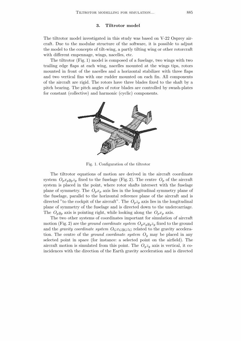
The tiltrotor model investigated in this study was based on V-22 Osprey air-craft. Due to the modular structure of the software, it is possible to adjustthe model to the concepts of tilt-wing, a partly tilting wing or other rotorcraftwith different empennage, wings, nacelles, etc.The tiltrotor (Fig. 1) model is composed of a fuselage, two wings with two

trailing edge flaps at each wing, nacelles mounted at the wings tips, rotorsmounted in front of the nacelles and a horizontal stabilizer with three flapsand two vertical fins with one rudder mounted on each fin. All componentsof the aircraft are rigid. The rotors have three blades fixed to the shaft by apitch bearing. The pitch angles of rotor blades are controlled by swash-platesfor constant (collective) and harmonic (cyclic) components.

Fig. 1. Configuration of the tiltrotor

The tiltrotor equations of motion are derived in the aircraft coordinatesystem Opxpypzp fixed to the fuselage (Fig. 2). The centre Op of the aircraftsystem is placed in the point, where rotor shafts intersect with the fuselageplane of symmetry. The Opxp axis lies in the longitudinal symmetry plane ofthe fuselage, parallel to the horizontal reference plane of the aircraft and isdirected ”to the cockpit of the aircraft”. The Opzp axis lies in the longitudinalplane of symmetry of the fuselage and is directed down to the undercarriage.The Opyp axis is pointing right, while looking along the Opxp axis.The two other systems of coordinates important for simulation of aircraft

motion (Fig. 2) are the ground coordinate system Ogxgygzg fixed to the groundand the gravity coordinate system OGxGyGzG related to the gravity accelera-tion. The centre of the ground coordinate system Og may be placed in anyselected point in space (for instance: a selected point on the airfield). Theaircraft motion is simulated from this point. The Ogzg axis is vertical, it co-incidences with the direction of the Earth gravity acceleration and is directed


Fig. 2. Systems of coordinates of an aircraft

along its positive value. The axes Ogxg and Ogyg lie in the horizontal plane,i.e. the plane perpendicular to the direction of gravity acceleration. The Ogxglies along the local geographical meridian pointing north, and the Ogyg axispoints east.The centre OG of the gravity system of coordinates coincides with the

centre of fuselage Op. The axis of the gravity system is parallel to the axisof the ground coordinate system. The gravity coordinate system is used fordescribing the position and attitude of the aircraft. The gravity system istranslated from the inertia system by the vector xG(t) = [xG(t), yG(t), zG(t)]

⊤,which is a function of time. The vector xG(t) describes the translation of thetiltrotor in space. It should be noted here that the point OG may not be thecentre of gravity of the aircraft.The relation between the gravity and the aircraft system of coordinates is

described by Euler’s angles of rotation. The relation between the coordinatesin both systems is given by an equation

xp = AG(Ψ,Θ,Φ)xG (3.1)

where the rotation matrix AG has the form

AG =(3.2)

=

cosΨ cosΘ sinΨ cosΘ − sinΘcosΨ sinΘ sinΦ− sinΨ cosΦ sinΨ sinΘ sinΦ+ cosΨ cosΦ cosΘ sinΦcosΨ sinΘ cosΦ+ sinΨ sinΦ sinΨ sinΘ cosΦ− cosΨ sinΦ cosΘ cosΦ

Aircraft motion is described by the vector

X = [V ,Ω,xg,Φ]⊤ = [U, V,W,P,Q,R, xg , yg, zg, Φ,Θ, Ψ ]

⊤ (3.3)

as a composition of four vectors:


– translation velocity V = [U, V,W ]⊤

– rotation (rates) Ω = [P,Q,R]⊤

– Euler’s angles written in a vector form Φ = [Φ,Θ, Ψ ]⊤

– translation of the aircraft relative to the ground xg = [xg, yg, zg]⊤.

3.1. Equation of motion

Equations of motion of the aircraft are derived using d’Alambert princi-ple, summing up at the point Op all loads (forces and moments) acting onthe fuselage, wings, control surfaces, nacelles, and rotors. The system of sixequations of motion is obtained, which may be grouped as two subsystems forforces and moments acting on the fuselage and wings (index p), two nacelles(indices n1, n2) and two rotors (indices r1, r2)

F p + F n1 + F n2 + F r1 + F r2 = 0(3.4)

M p +Mn1 +Mn2 +M r1 +M r2 = 0

Each element of the above equations consists of inertia, aerodynamic andgravity parts

Q() = [F (),M ()]⊤ = Q()i +Q()a +Q()g (3.5)

3.2. Inertia loads

The expression for inertia loads is obtained from the conservation of mo-mentum, which after performing some mathematical manipulations, may bewritten in the matrix form

Qpb = IpY p +ΩpIpY p (3.6)

where the tilt-rotor state vector Y p = [U, V,W,P,Q,R]⊤ is composed of com-

ponents of aircraft translation velocity and rates. The inertia matrix has theform

Ip =

mp 0 0 0 Szp −Syp0 mp 0 −Szp 0 Sxp0 0 mp Syp −Sxp 00 −Szp Syp Ixp −Ixyp −IxzpSzp 0 −Sxp −Ixyp Iyp −Iyzp−Syp Sxp 0 −Ixzp −Iyzp Izp

(3.7)


and the velocity matrix is

Ωp =

0 −R Q 0 0 0R 0 P 0 0 0−Q P 0 0 0 00 −W V 0 −R Q

W 0 −U R 0 P

−V U 0 −Q P 0

(3.8)

Expression (3.6) describes inertia loads acting on the fuselage and on parts ofthe rotorcraft fixed to it, i.e. wings and control surfaces.

For parts of the aircraft rotating relative to the fuselage, i.e. nacelles(Fig. 3) and rotors, the inertia loads are calculated as

Qmb = Im(Y p + Y m) + (Ωp +Ωm)Im(Y p + Y m) (3.9)

In (3.9), the inertia matrices of rotating elements are calculated in thefuselage system of coordinates.

Fig. 3. Nacelle coordinate systems

Additional velocity matrices Ωm are added, containing in a general case therates and velocities of these elements relative to the fuselage. In the tiltrotorcase, they have the form


Im =

mm 0 0 0 Szm −Sym0 mm 0 −Szm 0 Sxm0 0 mm Sym −Sxm 00 −Szm Sym Ixm −Ixym −IxzmSzm 0 −Sxm −Ixym Iym −Iyzm−Sym Sxm 0 −Ixzm −Iyzm Izm

(3.10)

Ωm =

0 −Rm Qm 0 0 0Rm 0 −Pm 0 0 0−Qm Pm 0 0 0 00 0 0 0 −Rm Qm0 0 0 Rm 0 −Pm0 0 0 −Qm Pm 0

The nonlinear parts of equation (3.9) contain all accelerations acting on therotating elements, including gyroscopic effects.

3.3. Gravity loads

The gravity forces and moments are calculated first in the centres of gravityof the fuselage and aircraft elements. Next, they are transformed to the cen-tre Op of the fuselage system of coordinates. The vector of gravity accelerationin the gravity system of coordinates has components

g = [0, 0, g]⊤ (3.11)

It is rotated with respect to the fuselage system of coordinates using the trans-formation

gp = AG(Ψ,Θ,Φ)g (3.12)

The masses of fuselage, wings and empennage are accounted for together andthe gravity loads of these parts are calculated as fuselage gravity loads

F pg = mpgp = mpAGg(3.13)

Mpg = rCG × F pg = rCG × (mpAGg)

where the vector rCG describes the position of C.G. of the fusela-ge/wings/empennage relative to Op. The positions of C.G. of other parts ofthe airplane in the local systems of coordinates are calculated as

rCG = rn + A(φ, θ, ψ)rnCG (3.14)

where: rn is the vector of C.G. of the given element relative to the fuselagecentre, A(φ, θ, ψ) – general description of the matrix of rotation of the local


system of coordinates (fixed to the element) relative to the fuselage system ofcoordinates (it should be defined separately for each rotating element of thetilt-rotor), rnCG – vector of the position of CG of the element in the localsystem of coordinates.

The gravity loads acting on other aircraft elements are transferred to thefuselage system of coordinates by using formulae

F ng = mngp = mnAGg(3.15)

Mng = [rn +A(φ, θ, ψ)rnCG]× F ng = [rn + A(φ, θ, ψ)rnCG]× [mnAGg]

3.4. Aerodynamics loads

In the generic model, two methods of calculation of quasi-steady aerody-namic loads are used: a 2D model for elongated elements composed of airfoilsand a 3D model for solid bodies.

Fig. 4. Two-dimensional flow model

The two dimensional flow (Fig. 4) is used for wings, rotor blades and hori-zontal and vertical stabilizers. For better description, some coordinate systemsare introduced:

– coordinate system of the mounting point of the element ONxNyNzN

– local airfoil coordinate systems Oaxayaza

– coordinate system fixed to the airfoil aerodynamic centre Oacxacyaczac

– coordinate system connected with the geometrically twisted airfoilOagxagyagzag

– coordinate system defined by the vector of velocity of the local airfoilOavxavyavzav

– coordinate system of local inflow of the airfoil OV xV yV zV .


The transformation of the mentioned above coordinate systems can be descri-bed as

xN = ry + rac + AagAavAaV xV = ry + rac + ArxV

where Ar = AagAavAaV .The elongated element is divided along the span for cross sections in which

the two dimensional flow is assumed. In each cross section, the instant totalflow velocity (Fig. 4) is calculated as

V ()i = A−1r()A

−1(V +Ω × r() − AGW +U () +∆W ()) (3.16)

taking into account the velocities of:

a) motion of the fuselage and their aircraft elements in the inertia coordi-nate system

b) motion of the air W due to wind, gusts, etc.

c) inflow due rotors and wings.

Ar() matrix is a substitute matrix describing rotations of the coordinate sys-tems in airfoil (Fig. 4) from the system of the mounting point of the element tothe system of local velocity inflow (Ar = AagAavAaV ). The inflow due rotorsand wings ∆W () is calculated as

∆W () = k()(V +Ω × r() − AGW +U ()) (3.17)

where k() is a coefficient assumed for a given element.On rotor blades, the rotor induced velocity U () obtained from Glauert’s

model is also taken into account while calculating flow velocity. Aerodynamicloads acting in the ”aerodynamic centre” (AC) of the cross sections are cal-culated using aerodynamic coefficients for the airfoil section obtained for theactual airfoil angle of attack α and deflection δ of flaps (if they exist) by atable look procedure. In the cross sections, the vectors of aerodynamic forcesand moments are calculated in the flow coordinate system as

dP = [dD, 0, dL]⊤ dM = [0, dM, 0]⊤ (3.18)

where:— drag

dD =1

2ρc(y)V 2a Cx(α, δ)dy (3.19)

— lift

dL =1

2ρc(y)V 2a Cz(α, δ)dy (3.20)

— moment

dM =1

2ρc2(y)V 2a Cmy(α, δ)dy (3.21)


Fig. 5. Three-dimensional airflow

The loads are transferred to the element local system of coordinates, integratedalong the span and transferred to the fuselage system of coordinates.

The fuselage and nacelles (Fig. 5) are treated as three-dimensional bodies.Aerodynamic loads, as in the 2D case, are calculated in the centre of local,flow coordinate system

P()a =1

2ρArV

2C()c(α, β)

(3.22)

M()a =1

2ρArRrV

2Cm()c(α, β)

using the local instant velocity V c = [Uc, Vc,Wc]⊤ in the body aerodynamic

centre. The angle of incidence α and angle of slip β are calculated as

α = a sinWc

√

U2c + V2c +W

2c

β = a sinVc

√

U2c + V2c

(3.23)

and the table look procedure is used for obtaining the aerodynamic coefficients.The loads from the flow system of coordinates are transformed to the elementsystem of coordinates using the rotation matrix

AV =

− cos β cosα − sin β cos β sinα− sin β cosα cos β sin β sinα− sinα 0 − cosα

(3.24)

Finally, as in the 2D case, the loads are transformed from the element localsystem of coordinates to the fuselage system of coordinates.


4. Details of modelling tiltrotor parts

4.1. Fuselage

The inertia loads acting on the fuselage are calculated from formula (3.6),gravity loads from (3.13) and the aerodynamic loads from (3.22). The iner-tia matrix covers the fuselage, wings and empennage – elements fixed to thefuselage.

4.2. Wings

The tiltrotor wings have prescribed planeform, twist and airfoil distribu-tion along the span. At each wing, there are two flaps (ailerons) controlledindividually. Flap deflection angles δw = [δw11, δw12, δw21, δw22]

⊤ form a partof control variables in the simulation of aircraft motion. The aerodynamic lo-ads are calculated using the 2D model. The induced velocities of rotors areincluded into velocity of wing airflow calculated in sections along the span.

4.3. Horizontal stabilizer

The horizontal stabilizer forms a part of the empennage and is mountedat the fuselage tail. There are three flaps (elevators) at the trailing edge of thestabiliser, controlled individually. The horizontal stabilizer may have arbitraryairfoil shape and twist angle distribution along the span. The aerodynamicloads are calculated using the 2D model. Influence of the induced velocity ofrotors is taken into account in the stabilizer sections along the stabilizer spanwith the time delay due to the distance travelled from the rotor to empennage.The elevator deflection angles, written as the vector δh = [δh1, δh2, δh3]

⊤ area part of the vector of control variables.

4.4. Vertical stabilizers

The vertical stabilizers are mounted at the tip of the horizontal stabilizer.There is one flap (rudder) at the trailing edge of each of the two stabilizers,controlled individually. The vertical stabilizers may have arbitrary airfoil sha-pe and twist angle distributions along the span. The aerodynamic loads arecalculated using the 2D model. Influence of the induced velocity of the rotorsis taken into account in the proper sections along the stabilizer span with thetime delay due to the distance travelled from the rotor to empennage. Therudder deflection angles δv = [δv1, δv2]

⊤ are a part of the vector of controlvariables.


4.5. Engine nacelles

The engine nacelles are placed at the tip of each wing. They may rotateabout the axis perpendicular to the fuselage plane of symmetry. The nacellesinertia loads are calculated using expression (3.10) and gravity loads usingexpression (3.15). Aerodynamic loads are calculated using the 3D model. Thevelocity of airflow around the nacelles contains inflow from the rotors and acomponent due to rotation of nacelles about the fuselage axis. The angle ofnacelle rotation τ is included into the set of control variables.

4.6. Rotors

The rotors rotation axes are perpendicular to the axis of nacelle rotationrelative to the fuselage. When the rotor axes are in the horizontal position, theright rotor rotates clockwise, and the left counter-clockwise looking from therear of the fuselage. For calculations of inertia loads, the rotors are treated asrotating discs and in the hub system of coordinates, the inertia matrices havethe form

Iri =

mri 0 0 0 0 00 mri 0 0 0 00 0 mri 0 0 00 0 0 0 0 00 0 0 0 0 00 0 0 0 0 Izri

(4.1)

The final form of inertia matrices of rotors (3.10)1 results from nacelle androtors rotation about the fuselage axis.

Each rotor has three blades mounted to the shaft by pitch bearings. Thepitch of the rotor blades is controlled by the swash-plate, resulting in collectiveand periodic control in the form

θij = θ0i + θ1i cos(

Ωit+2π

3j)

+ θ2i sin(

Ωit+2π

3j)

(4.2)

The blades may have arbitrary planeform, twist and airfoil distribution alongthe span. The aerodynamic loads are calculated using strip theory with qu-asisteady aerodynamic loads using the table-look procedure for calculations ofaerodynamic coefficient of airfoils (2D model described above). The inducedflow is calculated using Glauert’s model. The control of rotor swash-plates maybe written in the vector form Θ = [Θ01, Θ02, Θ11, Θ12, Θ21, Θ22]

⊤ containingthe sub-set of tiltrotor control variables.

The control vector of the tiltrotor

C = [τ, δw, δh, δv,Θ]⊤ (4.3)


consists of (respectively) tilt angle of nacelles, angles of deflection of ailerons,elevators and rudders, pitch control of rotors, which is 16 control states. Theangular velocity of the rotor is assumed constant.

5. Calculation of trim in steady flight

Including inertia loads into the general form of equations of motion, the tilt-rotor equations of motion have the form

IpY p +ΩpIpY p +2∑

i=1

(IniY ni +ΩniIniY ni) +2∑

i=1

(IriY ri +ΩriIriY ri) =

(5.1)

= Qpg +2∑

i=1

Qnig +2∑

i=1

Qrig +Qpa +2∑

i=1

Qnia +2∑

i=1

Qria

In a steady flight, the accelerations are zero and the equations of motion arereduced to a system of 6 algebraic equations

Q = −ΩpIpY p −2∑

i=1

(IniY ni +ΩniIniY ni)−2∑

i=1

(IriY ri +ΩriIriY ri) +

(5.2)

+Qpg +2∑

i=1

Qnig +2∑

i=1

Qrig +Qpa +2∑

i=1

Qnia +2∑

i=1

Qria = 0

For trim conditions the equations of motion have the general form

Q(V p,Ωp,Φ, τ, δw, δh, δv,Θ) = 0 (5.3)

The values of trim controls in a steady flight are calculated using theLevenberg-Marquardt method to minimise total loads (5.3) acting on the til-trotor. This approach (Miller, 2004) allows one to obtain the trim states forthe cases when the number of calculated trim parameters is arbitrary, i.e. less,equal or greater than the number of equations of motion.

Minimizing the nonlinear functions numerically leads to compution of localminima, which may not be the real solution of the trim from the physicalpoint of view. To avoid such cases, the total loads acting on the tiltrotor ina steady flight were monitored. Simulations of the tiltrotor flight were doneusing controls calculated in the trim procedure to prove that the parametersobtained by the minimisation method were correct.


5.1. Data for simulation

The aim of simulation performed in this study was to check the validity ofthe model and to get insight into tiltrotor behaviour in the trimmed state. Dataof V-22 were used in the simulation. A part of the design data was taken fromaccessible literature (e.g., Miller and Narkiewicz, 2003; [11]). For parameterswith no available data, the values were assumed as for corresponding parts ofa similar aircraft (Miller, 2004). Base dimensions of the simulated tiltrotor areshown in Fig. 6 (Miller and Narkiewicz, 2003) and given in Table 1.

Fig. 6. Dimensions of V-22

Table 1. Tiltrotor data

Rotor System

Number of blades 3

Blades tip speed m/s (fps) 201.75 (661.90)

Diameter m (ft) 11.58 (38.00)

Disc area m2 (ft2) 210.70 (2 268.00)

Weights

Take off kg (lbs) 15 032 (33 140)

Dimensions

Length, fuselage m (ft) 1 748 (57.33)

Width, rotors turning m (ft) 25.55 (83.33)

Width, horizontal stabilizer m (ft) 5.61 (18.42)

Height, nacelles fully vertical m (ft) 6.63 (21.76)

Height, vertical stabilizer m (ft) 5.38 (17.65)


5.2. Results of simulations

Before simulating motion of the complete tiltrotor, separate modules andcomplete codes were debugged. Next, for the tiltrotor data, the results of sim-plified cases were checked for consistency with the proper reactions on theinput. For instance, analysis of the influence of each control surfaces (Miller,2004; Miller and Narkiewicz, 2001) on the tiltrotor flight was done for theselected flight phases (Swertfager and Martin, 1992). The tiltrotor flight si-mulations were done for three tiltrotor flight modes: helicopter, airplane andconversion.

The longitudinal, symmetrical cases of the flight are presented in thispaper. The side velocity V , angular velocities P , Q, R roll Φ and yaw Ψ

angles as well as the rudder deflection angles δv = δv1 = δv2 were assu-med zero. The same values were assumed for the deflection of wing flapsδw = δw11 = δw12 = δw21 = δw22, angles of elevators δh = δh1 = δh2 = δh3 andcollective control of the rotor pitch Θ0 = Θ01 = Θ02 for flaps on the wingsand elevator. The longitudinal cyclic control of the rotor was assumed symme-trical and Θ1 = Θ11 = Θ12, whereas the lateral cyclic control unsymmetricalΘ2 = Θ21 = −Θ.

During the trim calculations for the assumed values of forward U andvertical W flight velocities, the tiltrotor pitch angle Θ, deflection of flaps onthe wing δw and elevators δh, collective Θ0 and cyclic Θ1 pitch of rotor bladesand the nacelle tilt angle τ were computed.

The airplane, conversion and helicopter modes of the tiltrotor flight wereconsidered.

The results of a steady flight in the airplane mode (horizontal with verticalclimb) are given in Fig. 7 - Fig. 10. The forward flight velocity was changedwithin the range U = 10-180m/s, and the vertical velocity was changed withinthe range W = −20-20m/s.

The tiltrotor pitch angle obtained from simulations was equal 0 for theassumed flight conditions, and it was not presented in graphs. The calculateddeflection angles of wing flaps (Fig. 7) and elevators (Fig. 8) did not exceedthe values of available control surface deflections of V-22.

Fig. 7. Deflection of flaps


Fig. 8. Deflection of elevators

The collective control of the rotor (Fig. 9) is almost proportional to forwardspeed. When the forward speed is low (below 60m/s), the minimal tilt angle ofnacelles (Fig. 10) assuring proper values of the lift is about 70. The deflectionof wing flaps is maximum for low forward speed, to balance the inclination oflift from the rotors. The deflection of elevators is maximum, when the aircraftis in the conversion mode because of the necessity to provide a proper tiltrotorpitch moment. It has the maximum value when the conversion stops and therotor axis is in the horizontal position.

Fig. 9. Collective pitch

Fig. 10. Tilt angle of nacelles

5.3. Steady forward flight with vertical climb in conversion mode

In the conversion mode, a steady forward flight with vertical climb velocitywith possibile deflection angle of the nacelle was simulated. The forward flightvelocity was changed within the range U = 20-180m/s.


As in the previous case, the values of calculated deflection angles of wingflaps (Fig. 11) and elevators (Fig. 12) do not exceed the values of availablecontrol for V-22. The collective pitch of rotor is approximately proportionalto forward speed. The deflection of wing flaps (Fig. 11) is maximum for lowforward speed. When the forward speed is low, the minimum tilt angle ofnacelles (Fig. 14) is about 55 assuring the proper aerodynamic lift. It becomessmaller (about 43) when the forward speed increases.




Fig. 14. Tilt angle of nacelles


5.4. Steady forward flight with vertical climb in helicopter mode

In the helicopter mode, a steady forward flight with vertical climb with thetilt angle of the nacelles 90 was simulated. The forward flight velocity waschanged within the range U = −70-70m/s. The vertical velocity was changedwithin the range W = −20-20m/s.


Fig. 16. Cyclic control (longitudinal)


For the assumed steady flight conditions, the negligible small value of pitchangle of the tiltrotor is obtained. The collective control of rotor swash-plates(Fig. 15) increases with the increase of vertical speed. The cyclic control ofrotor pitch (Fig. 16) varies in the opposite way: when the vertical speed in-creases, the pitch angle of tiltrotor is also stabilized. The inclination angles



of wing flaps (Fig. 17) and elevators (Fig. 18) obtained in calculations do notexceed available values for V-22. In the range of negative forward speed, theinfluence of flap deflection on tiltrotor motion is not substantial, but it beco-mes noticeable at positive forward speed greater than 10-20m/s. The sign ofdeflection of control surfaces depends on the direction of vertical speed.

5.5. Side flight in helicopter mode

In the side flight in the helicopter mode, the forward flight velocity waschanged within the range U = −70-70m/s, and the side flight velocity waschanged within the range V = −20-20m/s. The tiltrotor vertical velocity theW = 0. The lateral cyclic pitch control was symmetrical Θ1 = Θ11 = Θ12 andlongitudinal cyclic control – unsymmetrical Θ2 = Θ21 = −Θ22. The aircraftpitch and yaw angles, pitch and yaw rates and both rudder deflections wereassumed zero.

From equilibrium conditions, the roll angle of tiltrotor Φ, inclination anglesof wing flaps δw = δw11 = δw12 = δw21 = δw22, inclination angles of elevatorsδh = δh1 = δh2 = δh3 and collective control of the rotor swash-plate Θ0 =Θ01 = Θ02 were calculated. The results are shown in Fig. 19 - Fig. 24.

In these flight conditions, the tiltrotor roll angle depends on side velocity.The deflections of flaps and elevators are small. The value of the cyclic pitchcontrol depends on the value of side speed and its sign.





Fig. 22. Roll angle of tiltrotor

Fig. 23. Cyclic control (lateral)

Fig. 24. Cyclic control (longitudinal)


5.6. Stability and controllability

For stability analysis, of the tiltrotor the equations of motion are nume-rically linearized with respect to state and control variables for given trimvalues. This allows analysis of the control matrix and calculation of eigenva-lues and eigenvectors for examination stability. This option of model analysisallows one to investigate the stability and controllability of the aircraft.

For the assumed tiltrotor design data, both stability and controllabilityanalysis was made for the whole forward speed range of the tiltrotor. In therange of velocity considered, complex eigenvalues with negative real parts wereobtained only for low velocity of forward flight (from 60 to 70m/s), whenthe conversion mode occurs. In other forward speed, negative real parts ofeigenvalues were obtained. These results show that in the steady flight, theaircraft is stable in the whole range of flight velocities.

Analysing the control matrix, it may be stated that the control variablesinfluence the related loads with minor cross-coupling effects. For the airplanemode, this is summarized in Table 2.

Table 2. Controllability analysis in the airplane mode

LoadsControl elements

airplane mode transition helicopter mode

Fx rotor collectivepitch

nacelles tilt angle,rotor collectivepitch

rotor longitudinalcyclic pitch

Fy rudders (no lateralcyclic pitch)

rudders (no lateralcyclic pitch)

rotor lateral cyclicpitch

Fz flaps, elevators (notnacelles tilt norlongitudinal cyclicpitch used)

flaps, nacelles tilt,rotor collectivepitch, elevators(smaller influence)

rotor collective pitch

Mx flaps, elevators,rotor collectivepitch

deflection of flaps,rotor collectivecontrol

asymmetric rotorcollective pitch

My elevators (rotorlongitudinal cyclicpitch not used)

deflection ofelevators, rotorcollective control

rotor longitudinalcyclic pitch(symmetric)

Mz rotor collectivepitch, rudders

rotor collectivepitch, rudders

rotor collectivepitch, rotorlongitudinal cyclicpitch


5.7. Results of numerical simulations

For the calculated steady flight parameters, simulations of flight were car-ried out to check their accuracy. The steady flight in the airplane mode wassimulated for: U = 180m/s, V = W = P = Q = R = 0, Φ = Θ = Ψ = 0and the trim parameters obtained from calculations were: deflection of wingflaps δw = −6.75

, elevators δh = 7.23 and collective pitch of the rotor

Θ0 = 45.91.

The tiltrotor displacements are presented in Fig. 25 (horizontal) and inFig. 26 (vertical). The variations of attitude angles are very small (below 0.1).

Fig. 25. Horizontal displacement in the airplane mode

Fig. 26. Vertical displacement in the airplane mode

It can be seen that during 1800m distance, the flight altitude decreased byabout 0.1m and side translation was about 0.1m to the left. These values areattributed to numerical errors in calculation of the trim values. Similar resultswere obtained in the transition and helicopter modes.

6. Conclusions

The tiltrotor computer model was developed for flight simulation, trim stabi-lity and control analysis. The model is composed of rigid elements: fuselage,wings, empennage, rotors, but due to the modularity of the code these as-sumptions may be easily released. The design parameters of V-22 tiltrotorwere used for simulations. Some data of the tiltrotor had to be assumed, andthere was no possibility to compare the results of numerical simulations withthe flight data. On the grounds of results of calculations performed, it may beconcluded that the developed model of the tiltrotor works properly.


A tiltrotor is a complex rotorcraft, and several simplifying assumptionshad to be applied. They might be released by adjusting the model for specificneeds of a particular helicopter.

Acknowledgement

The research was carried out as a part of a project supported by the State Com-

mittee for Scientific Research ”The research on the control of tiltrotor in selected flight

stages”, grant No. 5T12C06724.

References

1. Cicale M., 2003, ERICA: the European tiltrotor design and critical technologyprojects, 29th European Rotorcraft Forum, Friedrichshafen, Germany

2. McVeigh M.A., Nagib H., Wood T., Kiedaisch J., Stalker A., Wy-gnanski I., 2004, Model and full scale tiltrotor download reduction tests usingactive flow control, 60th Annual Forum, 1, Baltimore, MD

3. McVicar J.S.G., Bradley R., 1992, A generic tilt-rotor simulation modelwith parallel implementation and partial periodic trim algorithm, 18th Euro-pean Rotorcraft Forum, Avignon, France

4. Miller M., 2004, The Control of Tiltrotor in Chosen Flight Stages, Ph.D.Thesis, Warsaw, Poland

5. Miller M., Narkiewicz J., 2001, Control of tiltrotor aircraft, 4th NationalRotorcraft Forum, Warsaw, Poland

6. Miller M., Narkiewicz J., 2003, Simulation of tiltrotor motion, 29th Euro-pean Rotorcraft Forum, Friedrichshafen, Germany

7. Nixon M.W. et al., 2003, Aeroelastic stability of a four-bladed semi-articulated soft-in-plane tiltrotor model, 59 AHS Forum, 110, Phoenix, AZ,USA

8. Polak D.R., George A.R., 1998, Flowfield and acoustic measurements froma model tiltrotor in hover, Journal of Aircraft, 35, 6, 921-929

9. Srinivas V., Chopra I., 1996, Validation of a comprehensive aeroelastic ana-lysis for tiltrotor aircraft, AHS 52nd Annual Forum, Washington, D.C., USA

10. Swertfager T.A., Martin S. Jr., 1992, The V-22 for SOF, 48th AmericanHelicopter Society Annual Forum, Washington, D.C.

11. V-22 Osprey Technical Specifications, http://www.boeing.com/rotorcraft/military/v22/v22spec.htm

12. Weakley J.M., Kleinhesselink K.M., Mason D.H., Mitchell D.G.,2003, Simulation evaluation of V-22 degraded-mode flying qualities, 59 AHSForum, 135, Phoenix, AZ, USA


Modelowanie tiltrotora dla symulacji w różnych stanach lotu

Streszczenie

Opracowano symulacyjny model statku powietrznego typu tiltrotor przeznaczonydo symulacji lotu oraz analizy osiągów, stabilności i sterowania. Model wiropłata zło-żony jest z kadłuba, skrzydeł, usterzenia ogonowego, gondoli silnikowych i wirników.Równania ruchu zostały uzyskane przez sumowanie obciążeń od sił bezwładności, gra-witacyjnych i aerodynamicznych działających na każdy element statku powietrznego.Obciążenia aerodynamiczne skrzydeł, stateczników i łopat wirników zostały obliczo-ne z zastosowaniem quasistacjonarnego modelu opływu. Do wyznaczania prędkościindukowanej wirników zastosowano model Glauerta. Wpływ strumienia zawirniko-wego na skrzydła i stateczniki jest obliczany z wykorzystaniem aktualnej wartościprędkości indukowanej wirników. Program do modelowania wiropłata został opraco-wany w środowisku MatLab. Program zbudowany jest z modułów obliczeń obciążeńposzczególnych elementów wiropłata, które wykorzystywane są również do wyznacza-nia warunków lotu ustalonego, stateczności i sterowności. Podczas pierwszego etapubadań wyznaczono warunki ustalonego lotu tiltrotora w różnych konfiguracjach, copozwoliło zbadać zachowanie i potwierdzić poprawność modelu.

Manuscript received February 9, 2006; accepted for print July 5, 2006

Documents

TILTROTOR MODELLING FOR SIMULATION IN VARIOUS FLIGHT