Uncertainty Quantification of Tiltrotor Whirl Flutter Aeroelastic Stabilityfrom Multibody Analysis

Federico Guerroni, Alessandro Cocco, Andrea Zanoni∗, Pierangelo Masarati.Politecnico di Milano, Milano - Italy

∗andrea.zanoni@polimi.it

AbstractTiltrotor aircraft maximum horizontal flight speed is limited by whirl flutter. Current research efforts focus on one sideon experimentally investigating on the stability margins through specialized wind tunnel test-beds, and on the other sideon developing efficient numerical tools, to both guide the development and gain information from experimental efforts.In this work, the development of TiPa, a software package providing a customizable interface to the general-purposemultibody dynamics solver MBDyn to provide a parametric tiltrotor model generation and investigation tool is presented.The tool is combined with DAKOTA, a state of the art Uncertainty Quantification (UQ) tool to form a complete aeroelasticstochastic analysis package. Two strategies for the parametric model generation are presented. One is based on thedefinition of complete MBDyn tiltrotor models while the other one relies on the generation of two different subsystems tobe assembled through a substructuring approach. Some promising early results and assessment are presented, togetherwith the expected future research direction.

1 INTRODUCTION

Tiltrotors, due to their capability of vertical takeoff and land-ing and high–speed forward flight, received increasing at-tention in the last several decades. Their design is matureenough to make possible their entrance in the civil air trans-port market [1].

Tiltrotor design is a challenging engineering task to themultipurpose missions to be accomplished by this aircraft.As a representative example, the case of whirl flutter is dis-cussed in this work. Whirl flutter, a specific type of aeroe-lastic flutter instability [2, 3], is a phenomenon that is knownto affect both turboprop and tiltrotor aircraft [4].

When a rotor mounted on a flexible structure rotates,the normal vibration modes associated to the elastic be-haviour of the supporting structure are merged into preces-sion modes. A point on the rotor axis of rotation draws cir-cular paths about its initial position, changing the way eachrotor blade perceive the incoming air speeds and generatinga new set of aerodynamic loads. When this phenomenon istriggered, such forces can lead to the divergence of the sys-tem response and to the whirl flutter instability [5].

Nowadays, the understanding of the phenomenon intiltrotor aircraft is still limited. Since many factors, for in-stance geometrical design, materials, actuators dynamics,can contribute to its occurrence, getting an accurate predic-tion of the aircraft aeroelastic behaviour can be very com-plicated.

The research group of the authors has been involvedin numerous research activities focused on the multibodyaeroelastic modeling of tiltrotors [6]. Parametric multibody

modeling of the vehicle has been used as the primary tool inorder to study the sensitivities that each design parameterplay on this phenomena.

Within this research frame, a MATLAB tool aimed at theautomatic generation of arbitrary tiltrotor multibody para-metric models, currently in development by the authors, ispresented. The tool has been called TiPa (Tiltrotor Para-metric model generator). It generates a model suitable tobe simulated with MBDyn (http://www.mbdyn.org/), ageneral purpose multibody software with well establishedaeroelastic capabilities.

Furthermore, TiPa is able to manage the interaction be-tween MBDyn and DAKOTA (https://dakota.sandia.gov/), an open source software under GNU LGPL licencewidely used in the research community to perform uncer-tainty quantification and optimization [7]. The aim is to de-velop a comprehensive tool for uncertainty quantification inrotorcraft analysis, focusing in particular on stability analysisof tiltrotor configurations.

The present work describes the design approach fol-lowed in the development of TiPa, describes its capabilitiesand presents some early results related to the WRATS [6]tiltrotor flutter analysis.

2 TIPA

The development of a parametric tiltrotor whirl flutter pre-diction tool is meant to satisfy specific investigation require-ments. Whirl flutter is an aeroelastic phenomenon affectedby a large number of factors. The need to understand how

Presented at the 46th European Rotorcraft Forum, Moscow, Russia, 8-11 September, 2020This work is licensed under the Creative Commons Attribution International License (CC BY). Copyright c© 2020 by author(s).

Page 1 of 13

each design feature influences a specific system aeroelasticbehaviour is crucial in gaining further insights on the originof instability phenomenon.

The easy adaptability of TiPa models allow this typeof investigation. First, it is designed to provide a semi-automatic model generator for an arbitrary user defined pro-protor configuration. The process is based on three in-put cards that store information about the system featuresand the required simulation properties. The software is de-signed to handle different amounts of input data in order tomatch the specific level of knowledge about the model con-figuration. Such information is used by TiPa to prepare inputfiles for MBDyn. It can, furthermore, directly manage theMBDyn simulation, in order to automatically complete theaeroelastic assessment of the current design. Finally, TiPaalso acts as a postprocessor for the response variables pro-vided by MBDyn analysis. Such tasks are designed to makeTiPa simulation flexible in order to be coupled with the ex-ternal Uncertainty Quantification software DAKOTA.

2.1 Parametric Modeling

The software requires the definition of a series of input vari-ables to be manipulated by TiPa internal schemes in orderto generate the desired geometries. These input parame-ters are accessible through textual (MATLAB format) inputcards:

1. the control card contains the parameters de-signed to control the current simulation, like

• which assembly components to generate andanalyze;

• the model structure;

• the air data for the aeroelastic assessment;

• the postprocessing operations;

2. the wing card stores the user defined informationrequired to model the wing subsystem;

3. the rotor card contains information about the rotorgeometrical, aerodynamic and structural definition.

As evidenced by the different input cards, TiPa handles themodel generation dividing the tiltrotor entire assembly intotwo parts (or subsystems): the wing and the rotor/pylon.This allows to write the rotor equations of motion in therotating frame, and apply the multiblade coordinates (MBC)transformation to the subsystem matrices.

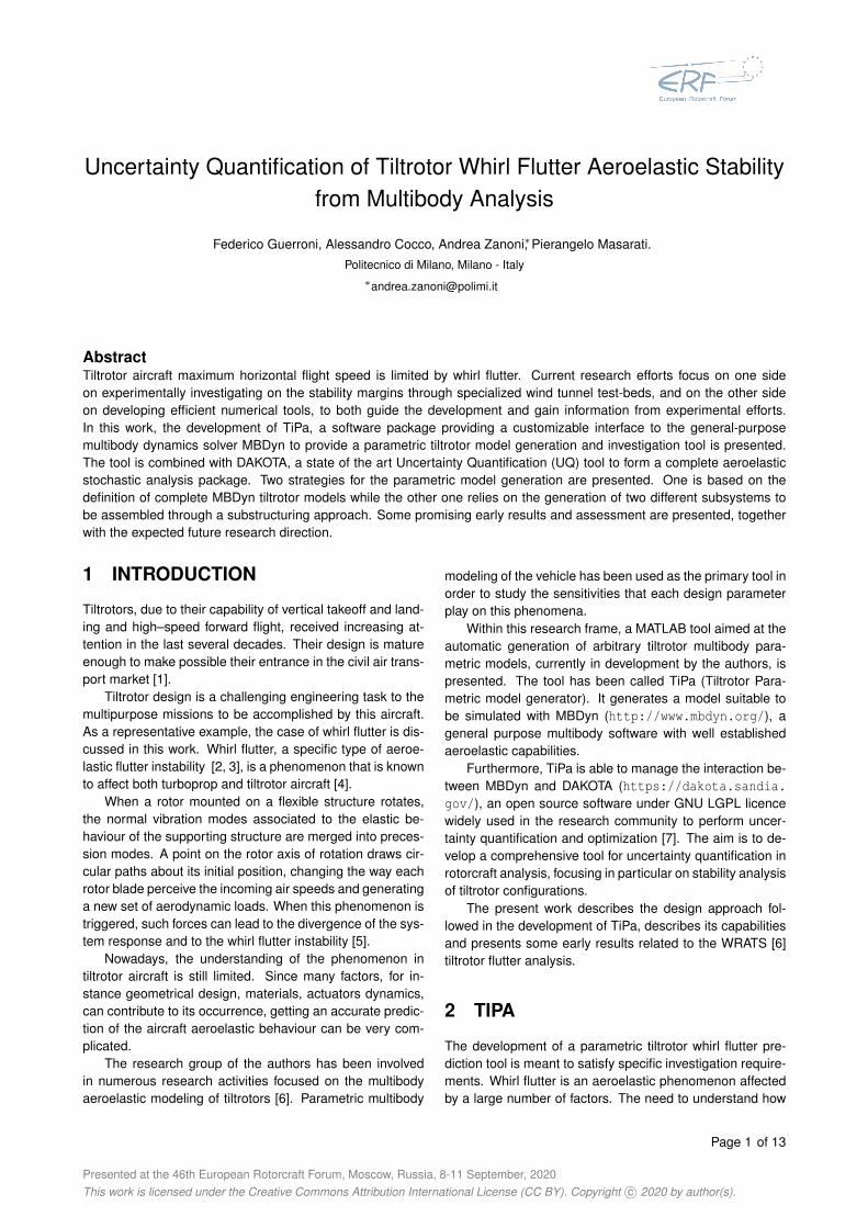
The wing subsystem definition and analysis is depictedgraphically in Fig. 1. Please note that in the figure, the directinteraction between the user and the solver elements is rep-resented with dashed lines, while all the other actions arerepresented by continuous lines. The TiPa preprocessormodule is responsible for transforming the user defined dataregarding the wing geometrical and structural parameters,contained in the wing card and regarding the requested

analysis type and conditions, contained in the controlcard, into information compatible with MBDyn and printingthe MBDyn input file.

control card

wing card

PREPROCESSOR

POSTPROCESSOR

MBDyn

wing MBDyn input le

wing MBDyn output les

MBDyn wingmatrices

wingeigenfrequenciesand eigenvectors

win

g a

naly

sis

USER

control card

wing card

PREPROCESSOR

POSTPROCESSOR

MBDyn

rotor MBDyn input le

rotor MBDyn output les

MBDyn rotormatrices

rotoreigenfrequenciesand eigenvectors

USERrotorcard

MBC TRANSFORMER

non-rotating frame MBDyn rotor matrices

non-rotating frameeigenfrequenciesand eigenvectors

roto

r an

aly

sis

Figure 1: TiPa wing and rotor submodels analyses flowcharts.

The input file is then provided to MBDyn to execute theuser defined requested simulation. TiPa makes extensiveuse of MBDyn eigenanalysis [8], since its output files storeinformation about the modelled multibody system equa-tions. The extraction of the wing subsystem matrices andmodal parameters is devolved to the TiPa postprocessormodule.

Page 2 of 13

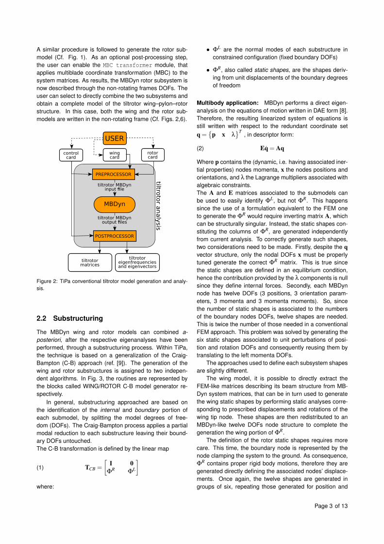
A similar procedure is followed to generate the rotor sub-model (Cf. Fig. 1). As an optional post-processing step,the user can enable the MBC transformer module, thatapplies multiblade coordinate transformation (MBC) to thesystem matrices. As results, the MBDyn rotor subsystem isnow described through the non-rotating frames DOFs. Theuser can select to directly combine the two subsystems andobtain a complete model of the tiltrotor wing–pylon–rotorstructure. In this case, both the wing and the rotor sub-models are written in the non-rotating frame (Cf. Figs. 2,6).

wing cardrotorcard

wing card

USER

tiltroto

r an

aly

sis

tiltrotormatrices

tiltrotoreigenfrequenciesand eigenvectors

PREPROCESSOR

MBDyn

tiltrotor MBDyn input le

tiltrotor MBDyn output les

control card

POSTPROCESSOR

Figure 2: TiPa conventional tiltrotor model generation and analy-sis.

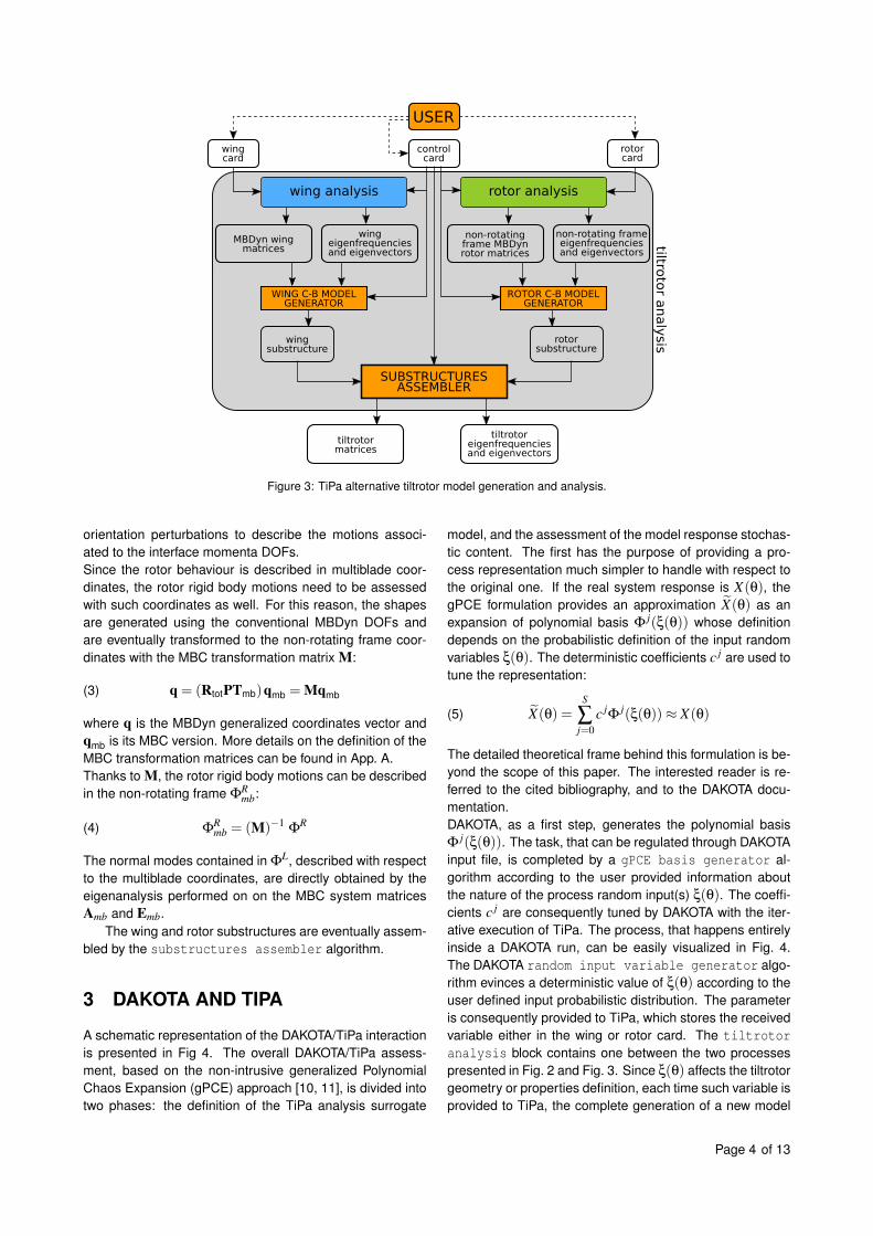
2.2 Substructuring

The MBDyn wing and rotor models can combined a-posteriori, after the respective eigenanalyses have beenperformed, through a substructuring process. Within TiPa,the technique is based on a generalization of the Craig-Bampton (C-B) approach (ref. [9]). The generation of thewing and rotor substructures is assigned to two indepen-dent algorithms. In Fig. 3, the routines are represented bythe blocks called WING/ROTOR C-B model generator re-spectively.

In general, substructuring approached are based onthe identification of the internal and boundary portion ofeach submodel, by splitting the model degrees of free-dom (DOFs). The Craig-Bampton process applies a partialmodal reduction to each substructure leaving their bound-ary DOFs untouched.The C-B transformation is defined by the linear map

(1) TCB =

[I 0

ΦR

ΦL

]where:

• ΦL are the normal modes of each substructure in

constrained configuration (fixed boundary DOFs)

• ΦR, also called static shapes, are the shapes deriv-

ing from unit displacements of the boundary degreesof freedom

Multibody application: MBDyn performs a direct eigen-analysis on the equations of motion written in DAE form [8].Therefore, the resulting linearized system of equations isstill written with respect to the redundant coordinate setq =

{p x λ

}T, in descriptor form:

(2) Eq = Aq

Where p contains the (dynamic, i.e. having associated iner-tial properties) nodes momenta, x the nodes positions andorientations, and λ the Lagrange multipliers associated withalgebraic constraints.The A and E matrices associated to the submodels canbe used to easily identify Φ

L, but not ΦR. This happens

since the use of a formulation equivalent to the FEM oneto generate the Φ

R would require inverting matrix A, whichcan be structurally singular. Instead, the static shapes con-stituting the columns of Φ

R, are generated independentlyfrom current analysis. To correctly generate such shapes,two considerations need to be made. Firstly, despite the qvector structure, only the nodal DOFs x must be properlytuned generate the correct Φ

R matrix. This is true sincethe static shapes are defined in an equilibrium condition,hence the contribution provided by the λ components is nullsince they define internal forces. Secondly, each MBDynnode has twelve DOFs (3 positions, 3 orientation param-eters, 3 momenta and 3 momenta moments). So, sincethe number of static shapes is associated to the numbersof the boundary nodes DOFs, twelve shapes are needed.This is twice the number of those needed in a conventionalFEM approach. This problem was solved by generating thesix static shapes associated to unit perturbations of posi-tion and rotation DOFs and consequently reusing them bytranslating to the left momenta DOFs.

The approaches used to define each subsystem shapesare slightly different.

The wing model, it is possible to directly extract theFEM-like matrices describing its beam structure from MB-Dyn system matrices, that can be in turn used to generatethe wing static shapes by performing static analyses corre-sponding to prescribed displacements and rotations of thewing tip node. These shapes are then redistributed to anMBDyn-like twelve DOFs node structure to complete thegeneration the wing portion of Φ

R.The definition of the rotor static shapes requires more

care. This time, the boundary node is represented by thenode clamping the system to the ground. As consequence,Φ

R contains proper rigid body motions, therefore they aregenerated directly defining the associated nodes’ displace-ments. Once again, the twelve shapes are generated ingroups of six, repeating those generated for position and

Page 3 of 13

control card

wing cardrotorcard

non-rotating frame MBDyn rotor matrices

non-rotating frameeigenfrequenciesand eigenvectors

rotor analysis

wing card

MBDyn wingmatrices

wingeigenfrequenciesand eigenvectors

wing analysis

USER

WING C-B MODELGENERATOR

ROTOR C-B MODELGENERATOR

wing substructure

rotor substructure

SUBSTRUCTURESASSEMBLER

tiltroto

r an

aly

sis

tiltrotormatrices

tiltrotoreigenfrequenciesand eigenvectors

Figure 3: TiPa alternative tiltrotor model generation and analysis.

orientation perturbations to describe the motions associ-ated to the interface momenta DOFs.Since the rotor behaviour is described in multiblade coor-dinates, the rotor rigid body motions need to be assessedwith such coordinates as well. For this reason, the shapesare generated using the conventional MBDyn DOFs andare eventually transformed to the non-rotating frame coor-dinates with the MBC transformation matrix M:

(3) q = (RtotPTmb)qmb = Mqmb

where q is the MBDyn generalized coordinates vector andqmb is its MBC version. More details on the definition of theMBC transformation matrices can be found in App. A.Thanks to M, the rotor rigid body motions can be describedin the non-rotating frame Φ

Rmb:

(4) ΦRmb = (M)−1

ΦR

The normal modes contained in ΦL, described with respect

to the multiblade coordinates, are directly obtained by theeigenanalysis performed on on the MBC system matricesAmb and Emb.

The wing and rotor substructures are eventually assem-bled by the substructures assembler algorithm.

3 DAKOTA AND TIPA

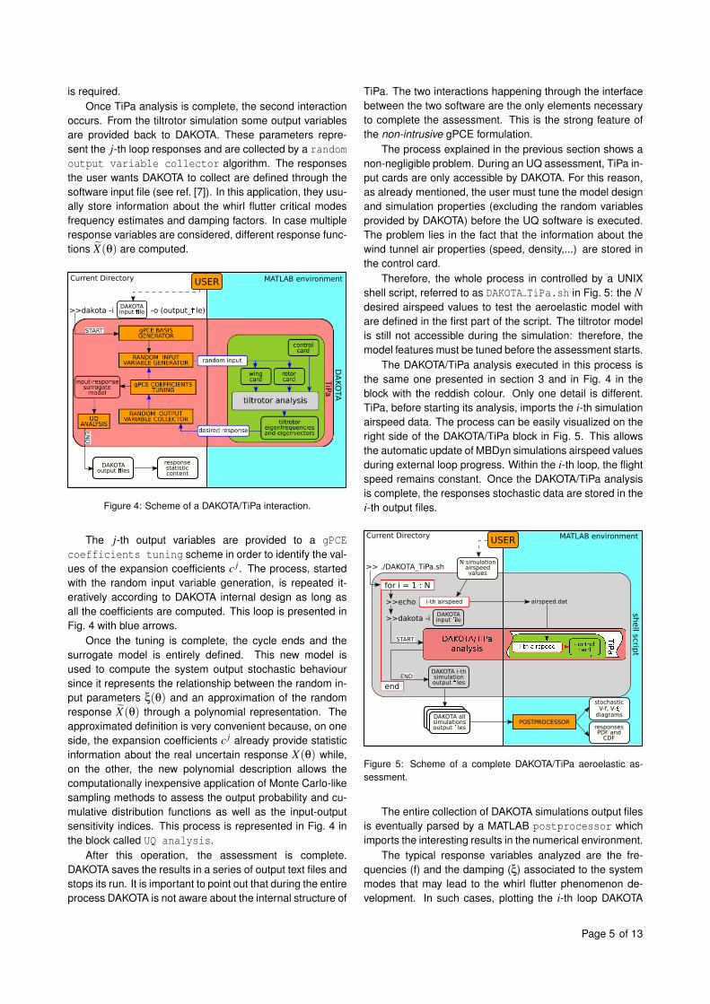
A schematic representation of the DAKOTA/TiPa interactionis presented in Fig 4. The overall DAKOTA/TiPa assess-ment, based on the non-intrusive generalized PolynomialChaos Expansion (gPCE) approach [10, 11], is divided intotwo phases: the definition of the TiPa analysis surrogate

model, and the assessment of the model response stochas-tic content. The first has the purpose of providing a pro-cess representation much simpler to handle with respect tothe original one. If the real system response is X(θ), thegPCE formulation provides an approximation X(θ) as anexpansion of polynomial basis Φ j(ξ(θ)) whose definitiondepends on the probabilistic definition of the input randomvariables ξ(θ). The deterministic coefficients c j are used totune the representation:

(5) X(θ) =S

∑j=0

c jΦ

j(ξ(θ))≈ X(θ)

The detailed theoretical frame behind this formulation is be-yond the scope of this paper. The interested reader is re-ferred to the cited bibliography, and to the DAKOTA docu-mentation.DAKOTA, as a first step, generates the polynomial basisΦ j(ξ(θ)). The task, that can be regulated through DAKOTAinput file, is completed by a gPCE basis generator al-gorithm according to the user provided information aboutthe nature of the process random input(s) ξ(θ). The coeffi-cients c j are consequently tuned by DAKOTA with the iter-ative execution of TiPa. The process, that happens entirelyinside a DAKOTA run, can be easily visualized in Fig. 4.The DAKOTA random input variable generator algo-rithm evinces a deterministic value of ξ(θ) according to theuser defined input probabilistic distribution. The parameteris consequently provided to TiPa, which stores the receivedvariable either in the wing or rotor card. The tiltrotoranalysis block contains one between the two processespresented in Fig. 2 and Fig. 3. Since ξ(θ) affects the tiltrotorgeometry or properties definition, each time such variable isprovided to TiPa, the complete generation of a new model

Page 4 of 13

is required.Once TiPa analysis is complete, the second interaction

occurs. From the tiltrotor simulation some output variablesare provided back to DAKOTA. These parameters repre-sent the j-th loop responses and are collected by a randomoutput variable collector algorithm. The responsesthe user wants DAKOTA to collect are defined through thesoftware input file (see ref. [7]). In this application, they usu-ally store information about the whirl flutter critical modesfrequency estimates and damping factors. In case multipleresponse variables are considered, different response func-tions X(θ) are computed.

Current Directory USER

DAKOTA input le>>dakota -i -o (output_ le)

wing card

DAKOTAoutput les

responsestatisticcontent

MATLAB environment

DA

KO

TA

Figure 4: Scheme of a DAKOTA/TiPa interaction.

The j-th output variables are provided to a gPCEcoefficients tuning scheme in order to identify the val-ues of the expansion coefficients c j. The process, startedwith the random input variable generation, is repeated it-eratively according to DAKOTA internal design as long asall the coefficients are computed. This loop is presented inFig. 4 with blue arrows.

Once the tuning is complete, the cycle ends and thesurrogate model is entirely defined. This new model isused to compute the system output stochastic behavioursince it represents the relationship between the random in-put parameters ξ(θ) and an approximation of the randomresponse X(θ) through a polynomial representation. Theapproximated definition is very convenient because, on oneside, the expansion coefficients c j already provide statisticinformation about the real uncertain response X(θ) while,on the other, the new polynomial description allows thecomputationally inexpensive application of Monte Carlo-likesampling methods to assess the output probability and cu-mulative distribution functions as well as the input-outputsensitivity indices. This process is represented in Fig. 4 inthe block called UQ analysis.

After this operation, the assessment is complete.DAKOTA saves the results in a series of output text files andstops its run. It is important to point out that during the entireprocess DAKOTA is not aware about the internal structure of

TiPa. The two interactions happening through the interfacebetween the two software are the only elements necessaryto complete the assessment. This is the strong feature ofthe non-intrusive gPCE formulation.

The process explained in the previous section shows anon-negligible problem. During an UQ assessment, TiPa in-put cards are only accessible by DAKOTA. For this reason,as already mentioned, the user must tune the model designand simulation properties (excluding the random variablesprovided by DAKOTA) before the UQ software is executed.The problem lies in the fact that the information about thewind tunnel air properties (speed, density,...) are stored inthe control card.

Therefore, the whole process in controlled by a UNIXshell script, referred to as DAKOTA TiPa.sh in Fig. 5: the Ndesired airspeed values to test the aeroelastic model withare defined in the first part of the script. The tiltrotor modelis still not accessible during the simulation: therefore, themodel features must be tuned before the assessment starts.

The DAKOTA/TiPa analysis executed in this process isthe same one presented in section 3 and in Fig. 4 in theblock with the reddish colour. Only one detail is different.TiPa, before starting its analysis, imports the i-th simulationairspeed data. The process can be easily visualized on theright side of the DAKOTA/TiPa block in Fig. 5. This allowsthe automatic update of MBDyn simulations airspeed valuesduring external loop progress. Within the i-th loop, the flightspeed remains constant. Once the DAKOTA/TiPa analysisis complete, the responses stochastic data are stored in thei-th output files.

wing card

Current Directory

end

wing card

DAKOTA allsimulationsoutput les

USER

for i = 1 : N

DAKOTA input le>>dakota -i

wing card

DAKOTA i-thsimulationoutput les

>> ./DAKOTA_TiPa.sh wing c\ard

N simulationairspeedvalues

i-th airspeed

START

END

POSTPROCESSOR

wing c\ard

stochasticV-f, V-

diagrams

wing c\ard

responsesPDF and

CDF

MATLAB environment

shell s

crip

t

airspeed.dat>>echo

Figure 5: Scheme of a complete DAKOTA/TiPa aeroelastic as-sessment.

The entire collection of DAKOTA simulations output filesis eventually parsed by a MATLAB postprocessor whichimports the interesting results in the numerical environment.

The typical response variables analyzed are the fre-quencies (f) and the damping (ξ) associated to the systemmodes that may lead to the whirl flutter phenomenon de-velopment. In such cases, plotting the i-th loop DAKOTA

Page 5 of 13

responses characterizations over the i-th airspeed valuesprovides a stochastic visualization of the V - f and V -ξ di-agrams. DAKOTA also outputs the responses’ ProbabilityDensity Functions (PDF), the Cumulative Distribution Func-tions (CDF) and the Sobol indices estimates, providing in-formation about how each input parameter affects a givenresponse function.

4 APPLICATIONS

Two examples of DAKOTA/TiPa analyses are shown in thefirst part this section. The assessments have been per-formed on a simplification of the three bladed stiff in-planeversion of the WRATS model, generated entirely with TiPa.Please note that such model represents a simpler versionof the original WRATS test-bed. In this part, the tested tiltro-tor is generated entirely in MBDyn through the conventionalmodelling approach.

In the second part, instead, some insight about the al-ternative modeling approach described in Section 2.2) ispresented. Despite the method showing some interestingand encouraging early results, its validation, at this stage ofthe development, is not complete yet. The state of the art,and the steps that led to the validation of most of the entireprocedure, are presented along with the description of thepath to complete the assessment of the process in futureresearch campaigns.

4.1 The WRATS model

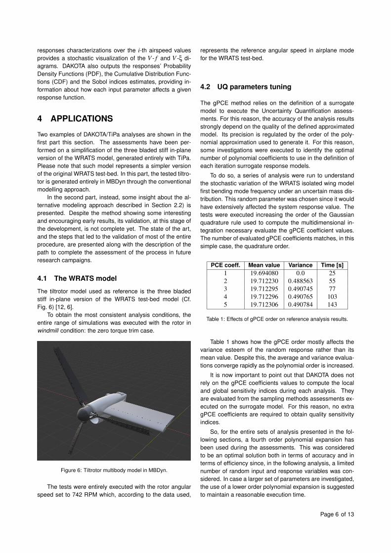
The tiltrotor model used as reference is the three bladedstiff in-plane version of the WRATS test-bed model (Cf.Fig. 6) [12, 6].

To obtain the most consistent analysis conditions, theentire range of simulations was executed with the rotor inwindmill condition: the zero torque trim case.

Figure 6: Tiltrotor multibody model in MBDyn.

The tests were entirely executed with the rotor angularspeed set to 742 RPM which, according to the data used,

represents the reference angular speed in airplane modefor the WRATS test-bed.

4.2 UQ parameters tuning

The gPCE method relies on the definition of a surrogatemodel to execute the Uncertainty Quantification assess-ments. For this reason, the accuracy of the analysis resultsstrongly depend on the quality of the defined approximatedmodel. Its precision is regulated by the order of the poly-nomial approximation used to generate it. For this reason,some investigations were executed to identify the optimalnumber of polynomial coefficients to use in the definition ofeach iteration surrogate response models.

To do so, a series of analysis were run to understandthe stochastic variation of the WRATS isolated wing modelfirst bending mode frequency under an uncertain mass dis-tribution. This random parameter was chosen since it wouldhave extensively affected the system response value. Thetests were executed increasing the order of the Gaussianquadrature rule used to compute the multidimensional in-tegration necessary evaluate the gPCE coefficient values.The number of evaluated gPCE coefficients matches, in thissimple case, the quadrature order.

PCE coeff. Mean value Variance Time [s]1 19.694080 0.0 252 19.712230 0.488563 553 19.712295 0.490745 774 19.712296 0.490765 1035 19.712306 0.490784 143

Table 1: Effects of gPCE order on reference analysis results.

Table 1 shows how the gPCE order mostly affects thevariance esteem of the random response rather than itsmean value. Despite this, the average and variance evalua-tions converge rapidly as the polynomial order is increased.

It is now important to point out that DAKOTA does notrely on the gPCE coefficients values to compute the localand global sensitivity indices during each analysis. Theyare evaluated from the sampling methods assessments ex-ecuted on the surrogate model. For this reason, no extragPCE coefficients are required to obtain quality sensitivityindices.

So, for the entire sets of analysis presented in the fol-lowing sections, a fourth order polynomial expansion hasbeen used during the assessments. This was consideredto be an optimal solution both in terms of accuracy and interms of efficiency since, in the following analysis, a limitednumber of random input and response variables was con-sidered. In case a larger set of parameters are investigated,the use of a lower order polynomial expansion is suggestedto maintain a reasonable execution time.

Page 6 of 13

4.3 DAKOTA/TiPa analysis results

This section presents some examples of DAKOTA/TiPaanalysis results. The assessments were performed us-ing the conventional TiPa tiltrotor whirl flutter modelling ap-proach, i.e. the parametric generation of the entire assem-bly within a single MBDyn model.

4.3.1 Single random input parameter propagation

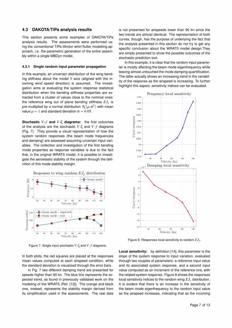
In this example, an uncertain distribution of the wing bend-ing stiffness about the model Y -axis (aligned with the in-coming wind speed direction) is assumed. The investi-gation aims at evaluating the system response statisticaldistribution when the bending stiffness properties are ex-tracted from a cluster of values close to the nominal ones:the reference wing out of plane bending stiffness EJy ispre-multiplied by a normal distribution N (µ,σ2) with meanvalue µ = 1 and standard deviation σ = 0.05.

Stochastic V - f and V -ξ diagrams: the first outcomesof the analysis are the stochastic V -ξ and V - f diagrams(Fig. 7). They provide a visual representation of how thesystem random responses (the beam mode frequenciesand damping) are assessed assuming uncertain input vari-ables. The collection and investigation of the first bendingmode properties as response variables is due to the factthat, in the original WRATS model, it is possible to investi-gate the aeroelastic stability of the system through the defi-nition of this mode stability margin.

30 40 50 60 70 80 90 100 110 120

5

5.5

6

30 40 50 60 70 80 90 100 110 120

0

0.02

0.04

Figure 7: Single input stochastic V -ξ and V - f diagrams.

In both plots, the red squares are placed at the responsesmean values computed at each airspeed condition, whilethe standard deviation is visualized through the error bars.

In Fig. 7 two different damping trend are presented forspeeds higher than 90 kn. The blue line represents the ex-pected trend, as found in previously validated work on themodeling of the WRATS (Ref. [13]). The orange and blackone, instead, represents the stability margin derived fromits simplification used in the assessments. The real data

is not presented for airspeeds lower than 90 kn since thetwo trends are almost identical. The representation of bothcurves, though, has the purpose of underlying the fact thatthe analysis presented in this section do not try to get anyspecific conclusion about the WRATS model design.Theyare simply presented to show the possible outcomes of thestochastic prediction tool.

In this example, it is clear that the random input parame-ter is mostly affecting the beam mode eigenfrequency whileleaving almost untouched the mode damping quantification.The latter actually shows an increasing trend in the variabil-ity of the response as the airspeed is increasing. To furtherhighlight this aspect, sensitivity indices can be evaluated.

Figure 8: Responses local sensitivity to random EJy.

Local sensitivity: by definition [14], this parameter is theslope of the system response to input variation, evaluatedthrough two couples of parameters: a reference input valueand its associated system response, and a second inputvalue computed as an increment of the reference one, withthe related system response. Figure 8 shows the responseslocal sensitivity indices to the random wing EJy distribution.It is evident that there is an increase in the sensitivity ofthe beam mode eigenfrequency to the random input valueas the airspeed increases, indicating that as the incoming

Page 7 of 13

wind speed rises, if the same perturbation in the system in-put is introduced, the evinced eigenfrequency value derivedfrom the perturbed input tends to increase. The dampingassociated local sensitivity indices have a magnitude sig-nificantly lower than the frequency ones. The interestingfeature of the damping local sensitivity trend, though, is rep-resented by the change of sign of such sensitivity indices asthe airspeed increases. This means that for the same posi-tive increase of the input variable, the beam mode dampingvalue is either increased (at about 30 kn) or decreased (atall the other tested speeds). This provides a very useful in-sight about the direction of the system response at differentspeeds.

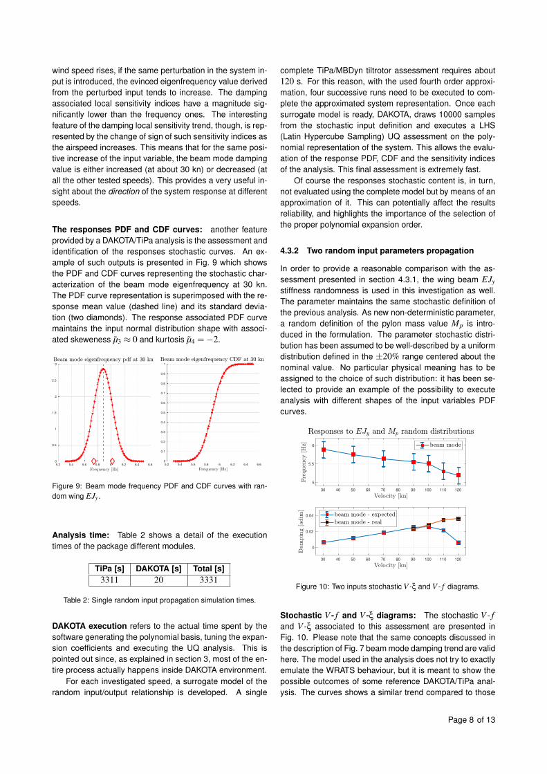
The responses PDF and CDF curves: another featureprovided by a DAKOTA/TiPa analysis is the assessment andidentification of the responses stochastic curves. An ex-ample of such outputs is presented in Fig. 9 which showsthe PDF and CDF curves representing the stochastic char-acterization of the beam mode eigenfrequency at 30 kn.The PDF curve representation is superimposed with the re-sponse mean value (dashed line) and its standard devia-tion (two diamonds). The response associated PDF curvemaintains the input normal distribution shape with associ-ated skeweness µ3 ≈ 0 and kurtosis µ4 =−2.

Figure 9: Beam mode frequency PDF and CDF curves with ran-dom wing EJy.

Analysis time: Table 2 shows a detail of the executiontimes of the package different modules.

TiPa [s] DAKOTA [s] Total [s]3311 20 3331

Table 2: Single random input propagation simulation times.

DAKOTA execution refers to the actual time spent by thesoftware generating the polynomial basis, tuning the expan-sion coefficients and executing the UQ analysis. This ispointed out since, as explained in section 3, most of the en-tire process actually happens inside DAKOTA environment.

For each investigated speed, a surrogate model of therandom input/output relationship is developed. A single

complete TiPa/MBDyn tiltrotor assessment requires about120 s. For this reason, with the used fourth order approxi-mation, four successive runs need to be executed to com-plete the approximated system representation. Once eachsurrogate model is ready, DAKOTA, draws 10000 samplesfrom the stochastic input definition and executes a LHS(Latin Hypercube Sampling) UQ assessment on the poly-nomial representation of the system. This allows the evalu-ation of the response PDF, CDF and the sensitivity indicesof the analysis. This final assessment is extremely fast.

Of course the responses stochastic content is, in turn,not evaluated using the complete model but by means of anapproximation of it. This can potentially affect the resultsreliability, and highlights the importance of the selection ofthe proper polynomial expansion order.

4.3.2 Two random input parameters propagation

In order to provide a reasonable comparison with the as-sessment presented in section 4.3.1, the wing beam EJystiffness randomness is used in this investigation as well.The parameter maintains the same stochastic definition ofthe previous analysis. As new non-deterministic parameter,a random definition of the pylon mass value Mp is intro-duced in the formulation. The parameter stochastic distri-bution has been assumed to be well-described by a uniformdistribution defined in the ±20% range centered about thenominal value. No particular physical meaning has to beassigned to the choice of such distribution: it has been se-lected to provide an example of the possibility to executeanalysis with different shapes of the input variables PDFcurves.

30 40 50 60 70 80 90 100 110 120

5

5.5

6

30 40 50 60 70 80 90 100 110 120

0

0.02

0.04

Figure 10: Two inputs stochastic V -ξ and V - f diagrams.

Stochastic V - f and V -ξ diagrams: The stochastic V - fand V -ξ associated to this assessment are presented inFig. 10. Please note that the same concepts discussed inthe description of Fig. 7 beam mode damping trend are validhere. The model used in the analysis does not try to exactlyemulate the WRATS behaviour, but it is meant to show thepossible outcomes of some reference DAKOTA/TiPa anal-ysis. The curves shows a similar trend compared to those

Page 8 of 13

presented in Fig. 7. When the second random variable isintroduced, though, the responses standard deviation tendsto increase with respect to the case in which only one ap-pears. It is interesting to notice how, in this second analysis,the beam mode damping standard deviation increment asthe airspeed rises is more evident compared to the previ-ous case.

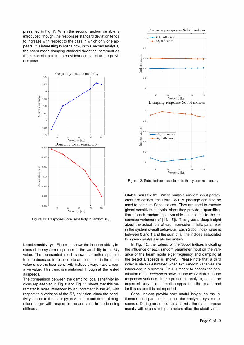
Figure 11: Responses local sensitivity to random Mp.

Local sensitivity: Figure 11 shows the local sensitivity in-dices of the system responses to the variability in the Mpvalue. The represented trends shows that both responsestend to decrease in response to an increment in the massvalue since the local sensitivity indices always have a neg-ative value. This trend is maintained through all the testedairspeeds.The comparison between the damping local sensitivity in-dices represented in Fig. 8 and Fig. 11 shows that this pa-rameter is more influenced by an increment in the Mp withrespect to a variation of the EJy definition, since the sensi-tivity indices to the mass pylon value are one order of mag-nitude larger with respect to those related to the bendingstiffness.

Figure 12: Sobol indices associated to the system responses.

Global sensitivity: When multiple random input param-eters are defines, the DAKOTA/TiPa package can also beused to compute Sobol indices. They are used to executeglobal sensitivity analysis, since they provide a quantifica-tion of each random input variable contribution to the re-sponses variance (ref [14, 15]). This gives a deep insightabout the actual role of each non-deterministic parameterin the system overall behaviour. Each Sobol index value isbetween 0 and 1 and the sum of all the indices associatedto a given analysis is always unitary.

In Fig. 12, the values of the Sobol indices indicatingthe influence of each random parameter input on the vari-ance of the beam mode eigenfrequency and damping atthe tested airspeeds is shown. Please note that a thirdindex is always estimated when two random variables areintroduced in a system. This is meant to assess the con-tribution of the interaction between the two variables to theresponses variance. In the presented analysis, as can beexpected, very little interaction appears in the results andfor this reason it is not reported.

Sobol indices provide very useful insight on the in-fluence each parameter has on the analyzed system re-sponse. During an aeroelastic analysis, the main purposeusually will be on which parameters affect the stability mar-

Page 9 of 13

gin the most. From Fig. 12, it is clear that randomness ofthe pylon mass has a larger influence on the beam modedamping variability with respect to the wing stiffness. This,in this simple test, may be due to the two different and ar-bitrary definitions provided to the input variables stochasticdefinitions. In a more realistic case, though, when two (ormore) comparable sources of randomness are introducedin the model, the information provided by the Sobol indicescan be very powerful and intuitive.

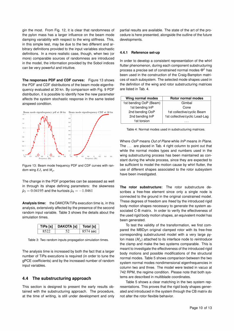
The responses PDF and CDF curves: Figure 13 showsthe PDF and CDF distributions of the beam mode eigenfre-quency evaluated at 30 kn. By comparison with Fig. 9 PDFdistribution, it is possible to identify how the new parameteraffects the system stochastic response in the same testedairspeed condition.

Figure 13: Beam mode frequency PDF and CDF curves with ran-dom wing EJy and Mp.

The change in the PDF properties can be assessed as wellin through its shape defining parameters: the skewnessµ3 = 0.04195 and the kurtosis µ4 =−1.0461

Analysis time: the DAKOTA/TiPa execution time is, in thisanalysis, extensively affected by the presence of the secondrandom input variable. Table 3 shows the details about thesimulation times.

TiPa [s] DAKOTA [s] Total [s]8522 52 8574 sec

Table 3: Two random inputs propagation simulation times.

The analysis time is increased by both the fact that a largernumber of TiPa executions is required (in order to tune thegPCE coefficients) and by the increased number of randominput variables.

4.4 The substructuring approach

This section is designed to present the early results ob-tained with the substructuring approach. The procedure,at the time of writing, is still under development and only

partial results are available. The state of the art of the pro-cedure is here presented, alongside the outline of the futuredevelopments.

4.4.1 Reference set-up

In order to develop a consistent representation of the whirlflutter phenomenon, during each component substructuringprocess a precise set of constrained normal modes Φ

L hasbeen used in the construction of the Craig-Bampton matri-ces of each subsystem. The selected mode shapes used inthe definition of the wing and rotor substructuring matricesare listed in Tab. 4.

Wing normal modes Rotor normal modes1st bending OoP (Beam) Gimbal

1st bending InP Cone2nd bending OoP 1st collective/cyclic Beam2nd bending InP 1st collective/cyclic Lead-Lag

1st torsion . . .

Table 4: Normal modes used in substructuring matrices.

Where OoP means Out of Plane while InP means In Plane.The . . . are placed in Tab. 4 right column to point out thatwhile the normal modes types and numbers used in thewing substructuring process has been maintained as con-stant during the whole process, since they are expected tobe sufficient to model the motion cause by whirl flutter, theuse of different shapes associated to the rotor subsystemhave been investigated.

The rotor substructure: The rotor substructure de-scribes a free-free element since only a single node isconnected to the ground in the original constrained model.These degrees of freedom are freed by the introduced rigidbody motion shapes necessary to generate the system as-sociated C-B matrix. In order to verify the effectiveness ofthe used rigid body motion shapes, an equivalent model hasbeen generated.

To test the validity of the transformation, we first com-pared the MBDyn original clamped rotor with its free-freecorresponding substructured model with a very large py-lon mass (Mp) attached to its interface node to reintroducethe clamp and make the two systems comparable. This ismeant to investigate the effectiveness of the introduced rigidbody motions and possible modifications of the structuralnormal modes. Table 5 shows comparison between the twosystem normal modes nondimensional eigenfrequencies incolumn two and three. The model were tested in vacuo at742 RPM, the regime condition. Please note that both sys-tems are described in multiblade coordinates.

Table 5 shows a clear matching in the two system rep-resentations. This proves that the rigid body shapes gener-ated and introduced in the system through the CB matrix donot alter the rotor flexible behavior.

Page 10 of 13

Mode name MBDyn model Subst. w large Mp MBDyn rotating[1/rev] [1/rev] [1/rev]

Gimbal≈ 0 ≈ 0 11.98 1.99 1

Cone 1.18 1.18 1.181st coll L-L 1.63 1.63 1.63

1st cyc L-L0.62 0.61 1.622.62 2.61 1.62

Table 5: Clamped MBDyn and substructured rotor modes comparison.

With the exact value of the pylon mass, the rotor sub-structured model eigenfrequencies slightly changes with re-spect to the clamped system ones. The modes shapes, aswell, adapt to the free interface condition. As example ofthis, in Fig. 14, the coning mode of the rotor substructureis presented. There, it is easy to identify the displacementof the mast and hub nodes with respect their initial position.This matches the expected behavior of the system with freeinterface. Among the eigenmodes associated to this sub-structured system some pure rigid body motions appear aswell.

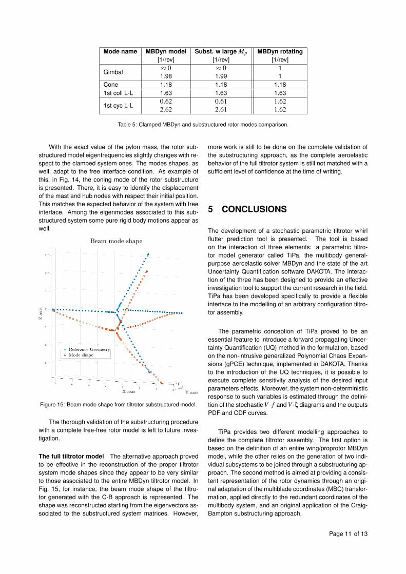
Figure 15: Beam mode shape from tiltrotor substructured model.

The thorough validation of the substructuring procedurewith a complete free-free rotor model is left to future inves-tigation.

The full tiltrotor model The alternative approach provedto be effective in the reconstruction of the proper tiltrotorsystem mode shapes since they appear to be very similarto those associated to the entire MBDyn tiltrotor model. InFig. 15, for instance, the beam mode shape of the tiltro-tor generated with the C-B approach is represented. Theshape was reconstructed starting from the eigenvectors as-sociated to the substructured system matrices. However,

more work is still to be done on the complete validation ofthe substructuring approach, as the complete aeroelasticbehavior of the full tiltrotor system is still not matched with asufficient level of confidence at the time of writing.

5 CONCLUSIONS

The development of a stochastic parametric tiltrotor whirlflutter prediction tool is presented. The tool is basedon the interaction of three elements: a parametric tiltro-tor model generator called TiPa, the multibody general-purpose aeroelastic solver MBDyn and the state of the artUncertainty Quantification software DAKOTA. The interac-tion of the three has been designed to provide an effectiveinvestigation tool to support the current research in the field.TiPa has been developed specifically to provide a flexibleinterface to the modelling of an arbitrary configuration tiltro-tor assembly.

The parametric conception of TiPa proved to be anessential feature to introduce a forward propagating Uncer-tainty Quantification (UQ) method in the formulation, basedon the non-intrusive generalized Polynomial Chaos Expan-sions (gPCE) technique, implemented in DAKOTA. Thanksto the introduction of the UQ techniques, it is possible toexecute complete sensitivity analysis of the desired inputparameters effects. Moreover, the system non-deterministicresponse to such variables is estimated through the defini-tion of the stochastic V - f and V -ξ diagrams and the outputsPDF and CDF curves.

TiPa provides two different modelling approaches todefine the complete tiltrotor assembly. The first option isbased on the definition of an entire wing/proprotor MBDynmodel, while the other relies on the generation of two indi-vidual subsystems to be joined through a substructuring ap-proach. The second method is aimed at providing a consis-tent representation of the rotor dynamics through an origi-nal adaptation of the multiblade coordinates (MBC) transfor-mation, applied directly to the redundant coordinates of themultibody system, and an original application of the Craig-Bampton substructuring approach.

Page 11 of 13

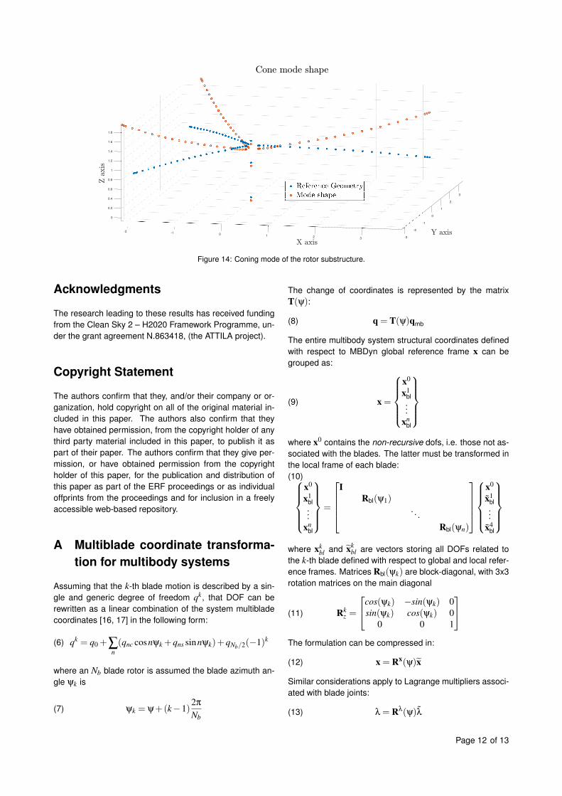
Figure 14: Coning mode of the rotor substructure.

Acknowledgments

The research leading to these results has received fundingfrom the Clean Sky 2 – H2020 Framework Programme, un-der the grant agreement N.863418, (the ATTILA project).

Copyright Statement

The authors confirm that they, and/or their company or or-ganization, hold copyright on all of the original material in-cluded in this paper. The authors also confirm that theyhave obtained permission, from the copyright holder of anythird party material included in this paper, to publish it aspart of their paper. The authors confirm that they give per-mission, or have obtained permission from the copyrightholder of this paper, for the publication and distribution ofthis paper as part of the ERF proceedings or as individualoffprints from the proceedings and for inclusion in a freelyaccessible web-based repository.

A Multiblade coordinate transforma-tion for multibody systems

Assuming that the k-th blade motion is described by a sin-gle and generic degree of freedom qk, that DOF can berewritten as a linear combination of the system multibladecoordinates [16, 17] in the following form:

(6) qk = q0 +∑n(qnc cosnψk +qns sinnψk)+qNb/2(−1)k

where an Nb blade rotor is assumed the blade azimuth an-gle ψk is

(7) ψk = ψ+(k−1)2π

Nb

The change of coordinates is represented by the matrixT(ψ):

(8) q = T(ψ)qmb

The entire multibody system structural coordinates definedwith respect to MBDyn global reference frame x can begrouped as:

(9) x =

x0

x1bl...

xnbl

where x0 contains the non-recursive dofs, i.e. those not as-sociated with the blades. The latter must be transformed inthe local frame of each blade:(10)

x0

x1bl...

xnbl

=

I

Rbl(ψ1). . .

Rbl(ψn)

x0

x1bl...

x4bl

where xk

bl and xkbl are vectors storing all DOFs related to

the k-th blade defined with respect to global and local refer-ence frames. Matrices Rbl(ψk) are block-diagonal, with 3x3rotation matrices on the main diagonal

(11) Rkz =

cos(ψk) −sin(ψk) 0sin(ψk) cos(ψk) 0

0 0 1

The formulation can be compressed in:

(12) x = Rx(ψ)x

Similar considerations apply to Lagrange multipliers associ-ated with blade joints:

(13) λ = Rλ(ψ)λ

Page 12 of 13

The MBDyn state vector q is described with respect to localblades reference frame through:

(14) q =

{xλ

}=

[Rx(ψ) 0

0 Rλ

]{xλ

}= Rtot(ψ) q

The overall transformation is given by

(15) q = (RtotPTmb)qmb = Tqmb

where P is a permutation matrix used to reorder the degreesof freedom in the shape q =

{pxλ

}T.

REFERENCES

[1] ACARE — Report of the Group of Personalities. Europeanaeronautics: a vision for 2020, January 2001.

[2] Eric Hathaway and Farhan Gandhi. Tiltrotor whirl flutter allevi-ation using actively controlled wing flaperons. AIAA Journal,44(11):2524–2534, 2006. doi:10.2514/1.18428.

[3] M. Mattaboni, P. Masarati, G. Quaranta, and P. Mantegazza.Multibody simulation of integrated tiltrotor flight mechan-ics, aeroelasticity and control. J. of Guidance, Control,and Dynamics, 35(5):1391–1405, September/October 2012.doi:10.2514/1.57309.

[4] Jirı Cecrdle. Whirl flutter-related certification according tofar/cs 23 and 25 regulation standards.

[5] Wilmer H Reed. Review of propeller-rotor whirl flutter. Na-tional Aeronautics and Space Administration, 1967.

[6] Pierangelo Masarati, David J Piatak, Giuseppe Quaranta,Jeffrey D Singleton, and Jinwei Shen. Soft-inplane tiltrotoraeromechanics investigation using two comprehensive multi-body solvers. Journal of the American Helicopter Society,53(2):179–192, 2008.

[7] Brian M Adams, WJ Bohnhoff, KR Dalbey, JP Eddy, MS El-dred, DM Gay, K Haskell, Patricia D Hough, and Laura PSwiler. Dakota, a multilevel parallel object-oriented frame-work for design optimization, parameter estimation, uncer-tainty quantification, and sensitivity analysis: version 5.0

user’s manual. Sandia National Laboratories, Tech. Rep.SAND2010-2183, 2009.

[8] P. Masarati. Direct eigenanalysis of constrained systemdynamics. Proc. IMechE Part K: J. Multi-body Dynamics,223(4):335–342, 2009. doi:10.1243/14644193JMBD211.

[9] Roy R. Craig, Jr. and Mervyn C. C. Bampton. Cou-pling of substructures for dynamic analysis. AIAA Journal,6(7):1313–1319, July 1968.

[10] Dongbin Xiu and George Em Karniadakis. The wiener–askeypolynomial chaos for stochastic differential equations. SIAMjournal on scientific computing, 24(2):619–644, 2002.

[11] Shuxing Yang, Fenfen Xiong, and Fenggang Wang. Poly-nomial chaos expansion for probabilistic uncertainty prop-agation. Uncertainty Quantification and Model Calibration,page 13, 2017.

[12] David J Piatak, Raymond G Kvaternik, Mark W Nixon,Chester W Langston, Jeffrey D Singleton, Richard L Bennett,and Ross K Brown. A wind-tunnel parametric investigation oftiltrotor whirl-flutter stability boundaries. 2001.

[13] J. Shen, P. Masarati, D. J. Piatak, M. W. Nixon, J. D. Sin-gleton, and B. Roget. Modeling a stiff-inplane tiltrotor usingtwo multibody analyses: a validation study. In American He-licopter Society 64th Annual Forum, Montreal, Canada, April29–May 1 2008.

[14] Jerome Morio. Global and local sensitivity analysis meth-ods for a physical system. European journal of physics,32(6):1577, 2011.

[15] Ilya M Sobol. Global sensitivity indices for nonlinear mathe-matical models and their monte carlo estimates. Mathemat-ics and computers in simulation, 55(1-3):271–280, 2001.

[16] Robert P. Coleman. Theory of self-excited mechanical oscil-lations of hinged rotor blades. ARR 3G29, NACA, July 1943.

[17] KH Hohenemser and SK Yin. On the use of first order rotordynamics in multiblade coordinates. In 30th Annual NationalForum of the American Helicopter Society, Preprint No. 831,1974.

Page 13 of 13