Analysis of ecological time series with ARMA( ) modelscase.edu/artsci/biol/abbottlab/Things_files/Ives,Abbott... · Analysis of ecological time series with ARMA(p,q) models ... Corresponding

Ecology, 91(3), 2010, pp. 858–871� 2010 by the Ecological Society of America

Analysis of ecological time series with ARMA( p,q) models

ANTHONY R. IVES,1,3 KAREN C. ABBOTT,1,4 AND NICOLAS L. ZIEBARTH1,2

1Department of Zoology, University of Wisconsin, 430 Lincoln Drive, Madison, Wisconsin 53706 USA2Department of Economics, Northwestern University, 2001 Sheridan Road, Evanston, Illinois 60202 USA

Abstract. Autoregressive moving average (ARMA) models are useful statistical tools toexamine the dynamical characteristics of ecological time-series data. Here, we illustrate theutility and challenges of applying ARMA( p,q) models, where p is the dimension of theautoregressive component of the model, and q is the dimension of the moving averagecomponent. We focus on parameter estimation and model selection, comparing bothmaximum likelihood (ML) and restricted maximum likelihood (REML) parameterestimation. While REML estimation performs better (has less bias) than ML estimation forARMA( p,q) models with p ¼ 1 (as has been found previously), for models with p . 1 theperformance of the estimators is complicated by multimodal likelihood functions. Theresulting difficulties in estimation lead to our recommendation that likelihood functions beroutinely investigated when applying ARMA( p,q) models. To aid this investigation, weprovide MATLAB and R code for the ML and REML likelihood functions. We furtherexplore the consequences of measurement error, showing how it can be explicitly andimplicitly incorporated into estimation. In addition to parameter estimation, we also examinemodel selection for identifying the correct model dimensions ( p and q). Finally, we estimatethe characteristic return rate of the stochastic process to its stationary distribution, a quantitythat describes a key property of population dynamics, and investigate bias that results fromboth estimation and model selection. While fitting ARMA models to ecological time serieswith complex dynamics has challenges, these challenges can be surmounted, making ARMA auseful and broadly applicable approach.

Key words: autoregressive moving average (ARMA) models; estimation bias; model selection;restricted maximum likelihood (REML) parameter estimation; return time; stability.

INTRODUCTION

Studies of time-series data have been increasing in

both frequency and sophistication in the ecological

literature, and are used to address diverse ecological

questions. In conservation and stock management, time-

series analyses are used to assess population sizes and

whether these sizes are declining (Dennis et al. 1991,

Dennis and Taper 1994, Hilborn and Mangel 1997,

Fagan 2001, Mullon et al. 2005). Time-series analyses

are also used to quantify the strength of population

regulation, or the stability of natural population

dynamics (e.g., Kendall et al. 1999, Ives et al. 2003,

Sæther et al. 2005, Brook and Bradshaw 2006, Sibly et

al. 2007). Sophisticated techniques are available to

search for evidence of complex population dynamics

such as chaos or alternative states (Ellner and Turchin

1995, Bjornstad and Grenfell 2001, Dennis et al. 2001,

de Valpine and Hastings 2002), or to anticipate incipient

regime shifts in the dynamical character of ecological

systems (Scheffer and Carpenter 2003, Biggs et al. 2009).

Finally, time-series analyses using models tailored to

specific species or communities have been used to extract

demographic information such as reproduction rates,

strengths of interaction between species, and impacts of

environmental factors (Zeng et al. 1998, Coulson et al.

2001, Gross et al. 2005).

Here, we discuss statistical approaches and challenges

for fitting autoregressive moving average (ARMA)

models to ecological time series. The ARMA( p,q)

model (where p is the dimension of the autoregressive

component of the model, and q is the dimension of the

moving average component) is as follows (Box et al.

1994):

ðxt � lÞ ¼Xp

i¼1

biðxt�i � lÞ þXq

j¼0

ajet�j ð1Þ

where xt is a measure of population density at sample t,

l is a parameter giving the mean of the stationary

process, bi are the autoregressive coefficients, et is a

temporally independent random variable, and aj are themoving average coefficients. Generally, population

densities are log-transformed for analyses, so that Eq.

1 can be applied as a loglinear model of dynamics.

The autoregressive (AR) component of the model

(xt�i terms) can arise ecologically from delayed effects of

densities xt�i on per capita population growth rates.

Manuscript received 14 March 2009; revised 26 June 2009;accepted 29 June 2009. Corresponding Editor: A. M. Ellison.

3 E-mail: [email protected] Present address: Department of Ecology, Evolution and

Organismal Biology, Iowa State University, Ames, Iowa50011 USA.

858

These can occur, for example, in age- or stage-structured

populations in which juveniles born in one year do not

reproduce until several years in the future (Fromentin et

al. 2001, Lande 2002, Murdoch et al. 2002). Delayed

density dependence may also occur as the result of

interactions among species (Turchin 1990, Turchin and

Taylor 1992). For example, in simple predator–prey

models that generate population cycles, the time series of

prey (or predator) density exhibits a lagged density

dependence, because prey born in year t� 2 increase the

predator density in year t � 1, which in turn decreases

the prey density in year t. In fact, for any nonlinear

deterministic population model, Takens’ theorem states

that the dynamics of an n-dimensional system (e.g., n

interacting species) are completely captured by a single-

dimensional model (e.g., for the dynamics of a single

species) that includes no more than p ¼ 2n þ 1 lags

(Takens 1981). For linear models, it is easy to show that

only p ¼ n lags are needed (Royama 1992).

The moving average (MA) component of the model

(et�j terms) can arise from interactions among multiple

species in a similar manner as the delayed density

dependence in the AR component of the model. In fact,

for any nonlinear stochastic population model, Stark

and colleagues (Stark 1999, Stark et al. 2003) demon-

strated that an n-dimensional system is completely

captured by a single-dimensional model that includes

no more than p¼2nþ1 lags in density and q¼2n lags in

the process error et. For linear models, this reduces to p

¼ n AR lags and q ¼ n � 1 MA lags.

ARMA models have at least three general, possibly

overlapping uses in ecology. First, they can be used

when a researcher has one or a few time series in hand

and wants to investigate potential processes underlying

their dynamics. When performing detailed analyses on

the dynamics of a particular system, we generally

advocate for a research approach involving mechanistic

models tailored specifically for the system (Kendall et al.

1999). Nonetheless, fitting a simple ARMA model might

be useful as a first step, for example, identifying the

lagged structure of the data (i.e., values of p and q).

Because it is linear, the ARMA model is the simplest

model that includes lagged effects in both densities and

environmental (random) fluctuations. Although ecolog-

ical time series are unlikely to be linear, by the Wold

representation theorem (Wold 1938) any stochastic

process can be represented by a MA process that has

identical statistical moments, and under mild restrictions

a pure MA process can be written as an ARMA process

(Box et al. 1994). Therefore, although equation 1 is

linear, it can nonetheless be used to approximate any

nonlinear stochastic process. In practice, this might not

be a useful result, because the MA process representa-

tion may be infinite (q ¼ ‘) and the number of lags

required to well-approximate the dynamics with an

ARMA process may be too large to allow practical

model fitting. Even in situations of strongly nonlinear

dynamics, however, fitting a linear ARMA model to the

data may be valuable. For example, in a study

investigating nonlinear dynamical phenomena such as

chaos or alternative states, a best-fitting linear model

can serve as a null hypothesis against which to compare

the fits of nonlinear models. This provides a test for the

existence of complex dynamics that cannot be well-

explained by linear processes (e.g., Ives et al. 2008).

A second use for ARMA models is to give a

quantitative estimate of some qualitative descriptor of

dynamics. For example, an ARMA model could be used

to estimate the mean and variance of the stationary

distribution of a stochastic process, or some measure of

the ‘‘stability’’ of the process. In this case, the quantity in

question is a function of the ARMA coefficients biand/or aj, and we are more interested in this function

than the actual coefficients. We then judge our ability to

fit the ARMA model to data based on the bias and

precision of the estimates of this function rather than the

bias and precision of the estimates of the specific

coefficients. An informative summary measure of the

dynamics of a system is its characteristic return time, or

more precisely, the rate at which the stochastic process

approaches its stationary distribution (i.e., the distribu-

tion that a process settles to after sufficient time). The

characteristic return time gives a measure of the stability

of the stochastic process, with greater stability corre-

sponding to more rapid return to stationarity.

A third use for ARMA models is to conduct broad

surveys of multiple time-series data sets (e.g., Fagan

2001, Brook and Bradshaw 2006, Sibly et al. 2007,

Ziebarth et al. 2009). When analyzing large numbers of

time series from different sources and possibly hetero-

geneous systems (e.g., taxonomically diverse species), it

is not practical to construct separate mechanistic,

nonlinear models appropriate for each system. Instead,

ARMA models can be fit to all time series, and the

resulting fitted models used to compare them. In broad

surveys, we are likely to be interested in functions of

ARMA coefficients, like the characteristic return time

discussed above, rather than the coefficients themselves.

When comparing multiple data sets, the sample size is

the number of data sets (rather than the number of

points in any one data set). Therefore, we are more

concerned about bias than precision. While we would

like high precision in the individual estimates for each

time series, any imprecision will merely make it harder

to statistically infer patterns. Bias, on the other hand,

could give us false results. The importance of bias over

precision separates the use of ARMA models for broad

surveys from the other two uses of ARMA models that

we described above for which both bias and precision

are important.

Of the three general uses we just outlined, we will

focus primarily on the second and third in this paper.

Therefore, we will de-emphasize estimating the values of

coefficients relative to a function of the coefficients, the

characteristic return time of a stochastic process.

Furthermore, we will focus more on bias than precision.

March 2010 859ARMA TIME-SERIES MODELS

Our leaning in part reflects our pragmatic assessment of

available ecological time series. While a time series

covering 40 years might represent an ecologist’s entire

career, such time series are short for statistical purposes.

With short data sets, the precision of the estimates of

ARMA coefficients may be sufficiently poor that the

estimates are of little value. Nonetheless, estimates of

functions of the coefficients may be much more precise,

and comparisons among numerous data sets for which

precision is less important may still be insightful.

Finally, by restricting ourselves to ARMA models, we

will in general only consider stationary stochastic

processes, that is, processes that have a finite long-term

variance. This excludes the case often investigated in

population viability analyses in which populations are

possibly decreasing to extinction (Morris and Doak

2002).

Our goal here is to present statistical approaches to

fitting ARMA models and describe possible statistical

challenges that may be encountered. We first address

parameter estimation using both restricted maximum

likelihood (REML) and maximum likelihood (ML)

techniques. While there are other estimation ap-

proaches, for example corrected estimating equations

(Staudenmayer and Buonaccorsi 2005) and the Whittle

estimator (Hauser 1999), ML and REML techniques are

more widely used and available in standard statistical

software packages. Downward (towards zero) bias in the

estimates of the AR coefficients is a well-known problem

for AR(1) (Quenouille 1949, Kendall 1954), AR( p)

(Cheang and Reinsel 2000), and ARMA (McGilchrist

1989) models, and theoretical and simulation studies

(McGilchrist 1989, Cheang and Reinsel 2000, 2003,

Kang et al. 2003) generally show that REML estimates

are less biased than ML estimates. In addition to

exploring bias, we also illustrate difficulties with ML

and REML estimation caused when the likelihood

and restricted likelihood functions are multimodal.

Multimodality may cause standard statistical software

to fail to find the ML and REML parameter estimates,

and it may introduce a particular type of bias as the

global maximum of the likelihood or restricted likeli-

hood functions jumps among local maxima. We have

not found a discussion of multimodal likelihood

functions for ARMA models in the literature, possibly

because attention has been focused on models with few

lags ( p � 2, q � 1) and/or longer time series.

Second, we address the issue of measurement error.

Measurement error may contaminate time-series data,

generating lags in the MA component of a fitted model

and causing bias in the coefficient estimates (Shenk et al.

1998, Ives et al. 2003, Staples 2004, Staudenmayer and

Buonaccorsi 2005, Dennis et al. 2006, Buonaccorsi and

Staudenmayer 2009). Here, we investigate two ap-

proaches to incorporating measurement error into

ARMA models. First, we use the well-known result

that measurement error in an ARMA( p,q) model gives

rise or contributes to the first p MA coefficients (Box et

al. 1994:126). Therefore, if interest is in the AR

components of an ARMA model, an ARMA( p,p) (or

an ARMA( p,q) if q . p) will implicitly absorb the

measurement error into the MA component, leaving the

AR coefficients (at least in principle) uncontaminated by

measurement error (Staudenmayer and Buonaccorsi

2005, Dennis et al. 2006). Second, we incorporate

measurement error explicitly by assuming that the

standard error of the point estimates in a time series is

known and equal for all points (homoscedastic). For this

case, we use ‘‘pseudo-ML’’ and ‘‘pseudo-REML’’

estimators (Bell and Wilcox 1993, Staudenmayer and

Buonaccorsi 2005) to fit the ARMA model. We treat the

second approach with pseudo-ML and -REML estima-

tors as the standard against which we judge the first,

implicit, and easier approach to account for measure-

ment error. While Staudenmayer and Buonaccorsi

(2005) also make this comparison (and also consider a

corrected estimating equation approach), they do this

only for AR( p) models and only in detail for AR(1) and

AR(2) models.

Finally, we investigate order selection (the values of p

and q) for ARMA models. Generally, the order of an

appropriate ARMAmodel is not known for a given data

set, and there are several methods of model selection

that have been used to estimate p and q (Shibata 1976,

Liang et al. 1993, Potscher and Srinivasan 1994,

Galeano and Pena 2007). We focus here on order

selection using Akaike’s information criterion corrected

for small sample sizes (AICc; Hurvich and Tsai 1989),

which has been shown with simulation studies to give

relatively good estimates of ARMA model order

(Malgras and Debouzie 1997). Functions of coefficients,

such as the characteristic return time, are defined for

ARMA models of arbitrary order. Because we do not

know the true order of the model, estimating the

characteristic return time has to be performed in

conjunction with model selection; the characteristic

return time might be estimated as some value for one

ARMA model but another value for an ARMA model

of different order. Here, we explore two procedures,

estimating the characteristic return time for the best-

fitting model and using model averaging (Burnham and

Anderson 2002), and determine how well they perform

in estimating the true characteristic return time.

We illustrate these approaches first using three

example data sets of grouse populations and then using

simulations based on models fitted to the grouse data.

We focus on the challenges faced when fitting ARMA

models; we selected these grouse data sets specifically

because they present statistical challenges, and we focus

the simulations on detailing causes of the challenges.

STATISTICAL METHODS

Both REML and ML estimation for time-series data

can be implemented in standard statistical packages,

although for more complicated models (with p . 1 and q

. 1), these may have difficulties. We used the lme( )

ANTHONY R. IVES ET AL.860 Ecology, Vol. 91, No. 3

function in R with corARMA( ) to structure the

covariances to perform REML estimation (R

Development Core Team 2008). While this performed

well when p ¼ 1, it often failed for higher-order models

for two reasons. First, it often failed to converge,

making it necessary to attempt different starting values

for the likelihood maximization. Second, the REML

likelihood functions were often not unimodal, and there

is no guarantee that lme( ) will find the global maximum.

Searching for the global maximum was hampered by the

restriction for lme( ) that initial values for coefficients be

bounded between �1 and 1, even though the true

coefficient values may have considerably larger magni-

tude. For ML estimation we used the arima( ) function

in R. While this did not have the convergence problems

of lme( ), it often did not find the global maximum

likelihood when the likelihood function was multimodal.

Despite these problems, lme( ) and arima( ) are useful as

a first place to start analyses; example code using both

lme( ) and arima( ) is given in the Appendix.

To overcome these problems of standard software

routines, and to allow us to explore in more detail the

difficulties of fitting ARMA models, we wrote our own

code for the ARMA likelihood and restricted likelihood

functions that can be used for ML and REML

estimation; the derivation is given in the Appendix,

along with code for both MATLAB (MathWorks 2005)

and R. Although our code implements estimation

differently from arima( ) and lme( ), we confirmed that

it gives identical estimates when used for ML and

REML, respectively, in the cases where arima( ) and

lme( ) converged on the global maximum. Because the

code gives the likelihood and restricted likelihood

functions, it can be used with any maximization routine

that can overcome problems with finding a global

maximum when there are multiple local maxima, such

as simulated annealing (Kirkpatrick et al. 1983).

Furthermore, while ML estimation for ARMA models

generally uses a Kalman filter, as in arima( ) in R, and

REML estimation generally uses a linear mixed model

approach, as in lme( ) in R (although REML can be

performed with a Kalman filter; Tsimikas and Ledolter

1994, 1998), our implementation uses a linear mixed

model approach for both. For long time series this is not

as efficient as a Kalman filter for ML estimation, but for

short time series it may be faster due to the ability to

condense out two parameters that hence do not need to

be considered during maximization. Our code for ML

and REML estimation is almost identical, differing in a

single term in one line of code, making it clear how ML

and REML estimation differ.

In addition to estimating coefficients of ARMA

models, we also estimated a measure of the characteristic

return time of the stochastic process (Ives et al. 2003).

The characteristic return time is determined by ||k||(Appendix), the magnitude of the inverse of the

minimum root of the characteristic equation (Box et

al. 1994). This value depends only on the AR coefficients

of an ARMA model. To illustrate this measure, consider

the transition distribution, that is, the time-dependent

distribution of xt if the process is perturbed from the

stationary distribution. Letting x̄t denote the time-

dependent mean of the transition distribution, the

asymptotic return rate of x̄t to the mean of the stationary

distribution x̄‘ is given by jx̄t� x̄‘j¼ ||k||jx̄t�1� x̄‘j; thus,the larger the magnitude of ||k||, the slower the

asymptotic rate of return. As the process approaches

nonstationarity, ||k|| approaches 1 (although the esti-

mation methods we use assume stationarity, and

therefore estimates of ||k|| will always be less than 1).

For models for which k is complex, k¼ cr 6 cii, the AR

components of the model generate quasi-cyclic dynamics

whose characteristic period is given by 2p/ci. Even

though the estimates of the AR coefficients (bi ) of an

ARMA model might be poor, the estimates of ||k||might be good; this situation might arise if different sets

of coefficients produce similar ||k|| values, so the

statistical determination of a general feature of the

dynamics (the characteristic return time) might be

‘‘easier’’ than the estimation of the actual coefficients.

Data sets are often contaminated with measurement

error, and ignoring measurement error can lead to

incorrect inferences about the dynamical properties of

time series (Fuller 1996, Ives et al. 2003, Staudenmayer

and Buonaccorsi 2005, Dennis et al. 2006). The

ARMA( p,q) model modified to include measurement

error is

ðxt � lÞ ¼Xp

i¼1

biðxt�i � lÞ þXq

j¼0

ajet�j x�t ¼ xt þ m/t

ð2Þ

where xt is the ‘‘true’’ population density, and x�t is the

observed value with measurement error given by the

normal (0,1) random variable /t multiplied by m so that

the measurement error has standard deviation m. The

inclusion of measurement error adds MA components

for lags 1, . . . , p to the time series (Box et al. 1994:126).

For example, if the biological processes are given by an

ARMA(3,0) process, contamination with measurement

error will make the time series an ARMA(3,3) process. If

the biological processes are given by an ARMA(1,2)

process, then measurement error will not change the

order of the process, although it will contribute to the

MA(1) component.

This result gives a strategy for implicitly incorporating

measurement error when interest is limited to the AR

components of an ARMA model; fit models with q � p

and let the MA( p) components absorb the measurement

error (Staudenmayer and Buonaccorsi 2005). To assess

this approach, we compared it to an alternative method

(Appendix) for explicitly incorporating measurement

error using pseudo-ML and pseudo-REML estimation

(Bell and Wilcox 1993, Staudenmayer and Buonaccorsi

2005). To explicitly incorporate measurement error, we

assume that we know the standard error m of the


measurement error term m/t; this is equivalent to

assuming that all measurements in the time series have

the same standard error (for a full discussion of mea-

surement error, see Staudenmayer and Buonaccorsi

[2005]). To compare approaches, we assume that the

main goal of an analysis is to assess the characteristic

return time of an ARMA process, as determined by ||k||.We know measurement error in a model with AR lags

up to order p will cause MA lags up to p. Therefore, if

we fit an ARMA( p,p) model to the data set, are the

estimates of bi and ||k|| improved? If the implicit

incorporation of measurement error by using an

ARMA( p,p) performs nearly as well as the model

explicitly incorporating measurement error, this shows

the utility of the ARMA( p,p).

To identify the best-fitting ARMA( p,q) model (i.e.,

the best choices of p and q), we used Akaike’s

information criterion corrected for small sample sizes

(AICc; Hurvich and Tsai 1989, Malgras and Debouzie

1997, Burnham and Anderson 2002). We also estimated

||k|| in two ways. First, we estimated ||k|| from the single

AICc best-fitting model. Second, we took the average of

the estimates of ||k|| for all models, weighting these

estimates by their AICc weights (Burnham and

Anderson 2002). This gives a weighted consensus among

models of the estimate of ||k||.

DATA SETS

To illustrate ARMA model estimation and selection,

we chose three time series of grouse dynamics from 27

data sets analyzed in Williams et al. (2004). We initially

selected this grouse database because we knew the time

series showed cyclic dynamics, and we chose three of

these specifically because they presented statistical

challenges. Therefore, while these data sets serve to

illustrate the strengths and limitations of different

methods, they are not representative of data sets that

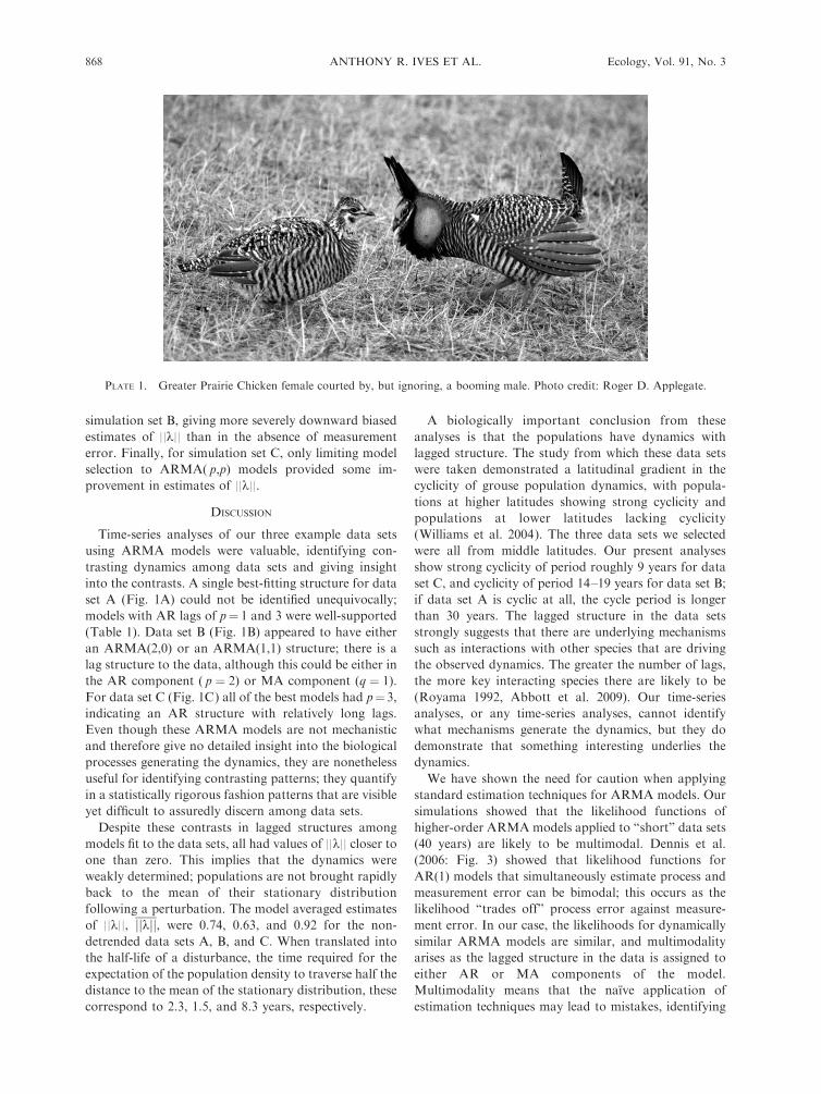
are generally available in the literature. Data set A is

from a Prairie Chicken population in Wisconsin, USA

(see Plate 1); data set B is from a Ruffed Grouse

population in the Upper Peninsula of Michigan; and

data set C is from a Sharp-tailed Grouse population in

South Dakota.

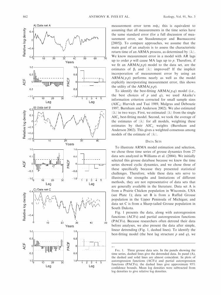
Fig. 1 presents the data, along with autoregression

functions (ACFs) and partial autoregression functions

(PACFs). Because researchers often detrend their data

before analyses, we also present the data after simple,

linear detrending (Fig. 1, dashed lines). To identify the

best-fitting model (the best lag structure p and q), we

FIG. 1. Three grouse data sets. In the panels showing the

time series, dashed lines give the detrended data. In panel (A),the dashed and solid lines are almost coincident. In plots ofautoregression functions (ACFs) and partial autoregressionfunctions (PACFs), the dashed lines give approximate 95%confidence bounds. Mean log densities were subtracted fromlog densities to give relative log densities.


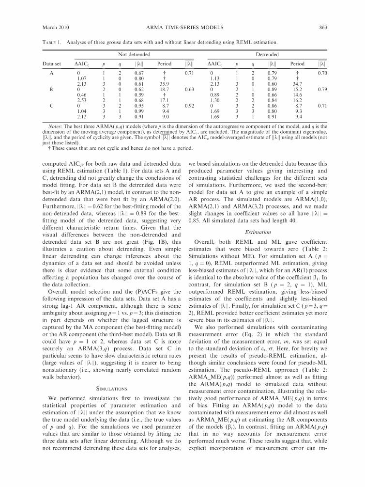
computed AICcs for both raw data and detrended data

using REML estimation (Table 1). For data sets A and

C, detrending did not greatly change the conclusions of

model fitting. For data set B the detrended data were

best-fit by an ARMA(2,1) model, in contrast to the non-

detrended data that were best fit by an ARMA(2,0).

Furthermore, ||k||¼0.62 for the best-fitting model of the

non-detrended data, whereas ||k|| ¼ 0.89 for the best-

fitting model of the detrended data, suggesting very

different characteristic return times. Given that the

visual differences between the non-detrended and

detrended data set B are not great (Fig. 1B), this

illustrates a caution about detrending. Even simple

linear detrending can change inferences about the

dynamics of a data set and should be avoided unless

there is clear evidence that some external condition

affecting a population has changed over the course of

the data collection.

Overall, model selection and the (P)ACFs give the

following impression of the data sets. Data set A has a

strong lag-1 AR component, although there is some

ambiguity about assigning p¼1 vs. p¼3; this distinction

in part depends on whether the lagged structure is

captured by the MA component (the best-fitting model)

or the AR component (the third-best model). Data set B

could have p ¼ 1 or 2, whereas data set C is more

securely an ARMA(3,q) process. Data set C in

particular seems to have slow characteristic return rates

(large values of ||k||), suggesting it is nearer to being

nonstationary (i.e., showing nearly correlated random

walk behavior).

SIMULATIONS

We performed simulations first to investigate the

statistical properties of parameter estimation and

estimation of ||k|| under the assumption that we know

the true model underlying the data (i.e., the true values

of p and q). For the simulations we used parameter

values that are similar to those obtained by fitting the

three data sets after linear detrending. Although we do

not recommend detrending these data sets for analyses,

we based simulations on the detrended data because this

produced parameter values giving interesting and

contrasting statistical challenges for the different sets

of simulations. Furthermore, we used the second-best

model for data set A to give an example of a simple

AR process. The simulated models are ARMA(1,0),

ARMA(2,1) and ARMA(3,2) processes, and we made

slight changes in coefficient values so all have ||k|| ¼0.85. All simulated data sets had length 40.

Estimation

Overall, both REML and ML gave coefficient

estimates that were biased towards zero (Table 2:

Simulations without ME). For simulation set A ( p ¼1, q ¼ 0), REML outperformed ML estimation, giving

less-biased estimates of ||k||, which for an AR(1) process

is identical to the absolute value of the coefficient b1. In

contrast, for simulation set B ( p ¼ 2, q ¼ 1), ML

outperformed REML estimation, giving less-biased

estimates of the coefficients and slightly less-biased

estimates of ||k||. Finally, for simulation set C ( p¼3, q¼2), REML provided better coefficient estimates yet more

severe bias in its estimates of ||k||.We also performed simulations with contaminating

measurement error (Eq. 2) in which the standard

deviation of the measurement error, m, was set equal

to the standard deviation of et, r. Here, for brevity we

present the results of pseudo-REML estimation, al-

though similar conclusions were found for pseudo-ML

estimation. The pseudo-REML approach (Table 2:

ARMA_ME( p,q)) performed almost as well as fitting

the ARMA( p,q) model to simulated data without

measurement error contamination, illustrating the rela-

tively good performance of ARMA_ME( p,q) in terms

of bias. Fitting an ARMA( p,p) model to the data

contaminated with measurement error did almost as well

as ARMA_ME( p,q) at estimating the AR components

of the models (bi ). In contrast, fitting an ARMA( p,q)

that in no way accounts for measurement error

performed much worse. These results suggest that, while

explicit incorporation of measurement error can im-

TABLE 1. Analyses of three grouse data sets with and without linear detrending using REML estimation.

Data set

Not detrended Detrended

DAICc p q jjkjj Period jjkjj DAICc p q jjkjj Period jjkjj

A 0 1 2 0.67 � 0.71 0 1 2 0.79 � 0.701.07 1 0 0.80 � 1.13 1 0 0.79 �2.13 3 0 0.61 35.9 2.13 3 0 0.60 34.7

B 0 2 0 0.62 18.7 0.63 0 2 1 0.89 15.2 0.790.46 1 1 0.59 � 0.89 2 0 0.66 14.62.53 2 1 0.68 17.1 1.30 2 2 0.84 16.2

C 0 3 2 0.95 8.7 0.92 0 3 2 0.86 8.7 0.711.04 3 1 0.99 9.4 1.69 3 3 0.80 9.32.12 3 3 0.91 9.0 1.69 3 1 0.91 9.4

Notes: The best three ARMA( p,q) models (where p is the dimension of the autoregressive component of the model, and q is thedimension of the moving average component), as determined by AICc, are included. The magnitude of the dominant eigenvalue,jjkjj, and the period of cyclicity are given. The symbol jjkjj denotes the AICc model-averaged estimate of jjkjj using all models (notjust those listed).

� These cases that are not cyclic and hence do not have a period.


prove estimation of the AR component of a model,

simply using an ARMA( p,p) model with extended MA

lags is a good strategy, especially in comparison to

ignoring the effects of measurement error.

In presenting these results and making this recom-

mendation, we have focused on bias in estimation rather

than precision (variance of the estimator). The intrusion

of measurement error noticeably decreased the precision

of estimates of ||k|| for simulation sets A and B. For

the case of the AR(1) process (simulation set A),

inclusion of known measurement error (Table 2:

ARMA_ME( p,q)) allowed more precise estimates of

||k|| in comparison to implicitly absorbing the measure-

ment error in the MA component of the ARMA(1,1)

model, as found by Staudenmayer and Buonaccorsis

(2005) in a more extensive set of simulations. This

phenomenon was investigated in detail by Knape (2008)

who demonstrated the identifiability problem of esti-

mating both measurement error and the autoregression

coefficient b1 of an AR(1) model. Somewhat surprising-

ly, the precision of the estimates of ||k|| for simulation

sets B and C, ARMA(2,1) and ARMA(3,2) models,

both with and without measurement error contamina-

tion is greater than for the AR(1) models of simulation

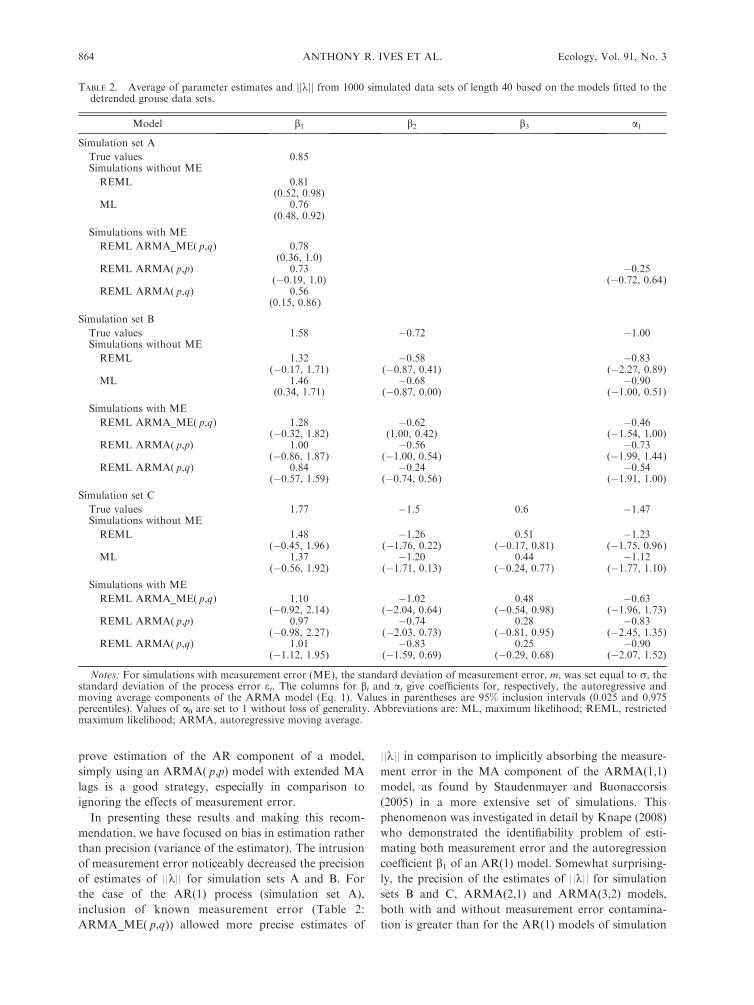
TABLE 2. Average of parameter estimates and jjkjj from 1000 simulated data sets of length 40 based on the models fitted to thedetrended grouse data sets.

Model b1 b2 b3 a1

Simulation set A

True values 0.85Simulations without ME

REML 0.81(0.52, 0.98)

ML 0.76(0.48, 0.92)

Simulations with ME

REML ARMA_ME( p,q) 0.78(0.36, 1.0)

REML ARMA( p,p) 0.73 �0.25(�0.19, 1.0) (�0.72, 0.64)

REML ARMA( p,q) 0.56(0.15, 0.86)

Simulation set B

True values 1.58 �0.72 �1.00Simulations without ME

REML 1.32 �0.58 �0.83(�0.17, 1.71) (�0.87, 0.41) (�2.27, 0.89)

ML 1.46 �0.68 �0.90(0.34, 1.71) (�0.87, 0.00) (�1.00, 0.51)

Simulations with ME

REML ARMA_ME( p,q) 1.28 �0.62 �0.46(�0.32, 1.82) (1.00, 0.42) (�1.54, 1.00)

REML ARMA( p,p) 1.00 �0.56 �0.73(�0.86, 1.87) (�1.00, 0.54) (�1.99, 1.44)

REML ARMA( p,q) 0.84 �0.24 �0.54(�0.57, 1.59) (�0.74, 0.56) (�1.91, 1.00)

Simulation set C

True values 1.77 �1.5 0.6 �1.47Simulations without ME

REML 1.48 �1.26 0.51 �1.23(�0.45, 1.96) (�1.76, 0.22) (�0.17, 0.81) (�1.75, 0.96)

ML 1.37 �1.20 0.44 �1.12(�0.56, 1.92) (�1.71, 0.13) (�0.24, 0.77) (�1.77, 1.10)

Simulations with ME

REML ARMA_ME( p,q) 1.10 �1.02 0.48 �0.63(�0.92, 2.14) (�2.04, 0.64) (�0.54, 0.98) (�1.96, 1.73)

REML ARMA( p,p) 0.97 �0.74 0.28 �0.83(�0.98, 2.27) (�2.03, 0.73) (�0.81, 0.95) (�2.45, 1.35)

REML ARMA( p,q) 1.01 �0.83 0.25 �0.90(�1.12, 1.95) (�1.59, 0.69) (�0.29, 0.68) (�2.07, 1.52)

Notes: For simulations with measurement error (ME), the standard deviation of measurement error, m, was set equal to r, thestandard deviation of the process error et. The columns for bi and ai give coefficients for, respectively, the autoregressive andmoving average components of the ARMA model (Eq. 1). Values in parentheses are 95% inclusion intervals (0.025 and 0.975percentiles). Values of a0 are set to 1 without loss of generality. Abbreviations are: ML, maximum likelihood; REML, restrictedmaximum likelihood; ARMA, autoregressive moving average.


set A. While imprecision may make the estimate of ||k||for a single data set uninformative, the relative lack of

bias means that this approach is still useful to make

comparisons among large numbers of data sets. Several

studies have investigated the dynamics of a large

collection of data sets (Fagan 2001, Brook and

Bradshaw 2006, Sibly et al. 2007, Ziebarth et al. 2009),

and for these studies the precision of the estimates is less

important when questions focus on the average dynam-

ics of the collections as a whole.

These estimation results are underlain by some

unpleasant statistical features. For simulation sets B

and C the likelihood functions were often multimodal

(Figs. 2 and 3). To find the global maximum for the

estimates in Table 2, we used both simulated annealing

(a maximization approach that is suitable for multi-

modal functions [Kirkpatrick et al. 1983]) and knowl-

edge of the true parameter values (the values of bi and ajused to simulate the data). The existence of multimodal

likelihood functions makes application of standard

routines to fit time-series data (such as lme( ) and

arima( ) in R) problematic.

For simulation set B, the likelihood functions were

often bimodal. Sometimes (e.g., Fig. 2A) the restricted

likelihood function was maximized at one of the local

peaks while the likelihood function was maximized at

the other. This led to very different REML and ML

parameter estimates even though the respective likeli-

hood functions were similar. Most of the differences in

REML and ML estimates observed in Table 2 were

caused by this type of phenomenon. Of 1000 simulations

37% had unimodal REML and ML likelihoods; for 35%

both REML and ML were bimodal; and for the

remainder only one was bimodal. The REML and ML

estimates differed due to the selection of different local

maxima in 6.3% of the simulations; roughly half of these

resulted when one likelihood function was bimodal and

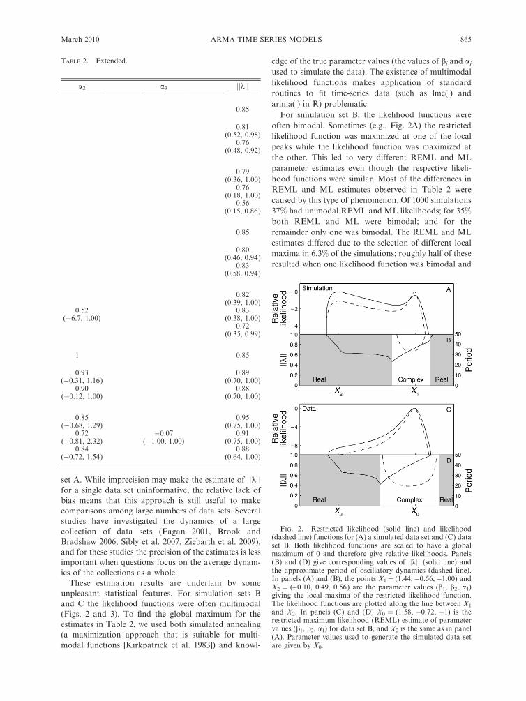
TABLE 2. Extended.

a2 a3 jjkjj

0.85

0.81(0.52, 0.98)

0.76(0.48, 0.92)

0.79(0.36, 1.00)

0.76(0.18, 1.00)

0.56(0.15, 0.86)

0.85

0.80(0.46, 0.94)

0.83(0.58, 0.94)

0.82(0.39, 1.00)

0.52 0.83(�6.7, 1.00) (0.38, 1.00)

0.72(0.35, 0.99)

1 0.85

0.93 0.89(�0.31, 1.16) (0.70, 1.00)

0.90 0.88(�0.12, 1.00) (0.70, 1.00)

0.85 0.95(�0.68, 1.29) (0.75, 1.00)

0.72 �0.07 0.91(�0.81, 2.32) (�1.00, 1.00) (0.75, 1.00)

0.84 0.88(�0.72, 1.54) (0.64, 1.00)

FIG. 2. Restricted likelihood (solid line) and likelihood(dashed line) functions for (A) a simulated data set and (C) dataset B. Both likelihood functions are scaled to have a globalmaximum of 0 and therefore give relative likelihoods. Panels(B) and (D) give corresponding values of ||k|| (solid line) andthe approximate period of oscillatory dynamics (dashed line).In panels (A) and (B), the points X1¼ (1.44,�0.56,�1.00) andX2 ¼ (�0.10, 0.49, 0.56) are the parameter values (b1, b2, a1)giving the local maxima of the restricted likelihood function.The likelihood functions are plotted along the line between X1

and X2. In panels (C) and (D) X0 ¼ (1.58, �0.72, �1) is therestricted maximum likelihood (REML) estimate of parametervalues (b1, b2, a1) for data set B, and X2 is the same as in panel(A). Parameter values used to generate the simulated data setare given by X0.


the global maximum did not match the location of the

single maximum in the other likelihood function, and

the other half occurred (as in Fig. 2A) when both

likelihood functions were bimodal with a mismatch

between their global maxima. While mismatches be-

tween REML and ML maxima were not common

(6.3%), the resulting estimates from REML and ML

were so different that they caused REML and ML

coefficient estimates to have differing degrees of bias

(Table 2).

For comparison, we also present the restricted

likelihood and likelihood functions for the actual data

set B (Fig. 2C). Both likelihood functions are very

similar, leading to similar REML and ML parameter

estimates. Thus, the analysis of the real data set B did

not suffer from the difficulties of the simulation data set

we selected for illustration (Fig. 2A).

It is important to ask what attributes of time series

cause these mismatches between REML and ML by

creating bimodal likelihood functions. In the vicinity of

the true parameter values (X1 in Fig. 2B), k is complex

with imaginary parts of 60.19i, implying quasi-cyclic

population dynamics with a period of 34 (¼2p/0.19). At

the alternative peak (X2) k is real, implying non-cyclic

dynamics. The simulated data set had 40 data points,

and therefore it is not surprising that support for a cycle

of period 34 can only be weak. In contrast, the real data

set B had coefficients corresponding to cycles of period

20 (Fig. 2D), and these were sufficiently well supported

to give unimodal likelihood functions.

The likelihood functions for simulation set C are

considerably more complex, having numerous local

maxima (Fig. 3); there are also regions of parameter

combinations for which the likelihood functions are not

defined, because the AR coefficients give nonstationary

dynamics (i.e., ||k|| . 1). We selected a single simulation

data set (Fig. 3A, B) to show an example in which

REML and ML estimation give very different parameter

estimates, corresponding to points X1 and X2, respec-

tively. Despite large differences in the parameter

estimates, however, the dynamics at parameter combi-

nations X1 and X2 are not strikingly different. At X1 the

characteristic roots of the ARMA model are 0.84 and

0.32 6 0.70i, and at X2 they are�0.78 and�0.26 6 0.34i.

The values of ||k|| are similar, 0.83 and 0.78, respective-

ly, and they show oscillations of period 9 and 19 years,

respectively. The most striking difference is the positive

real eigenvalue at point X1 and the negative real

eigenvalue at X2. These are coupled, however, with

values of a1¼�1.76 at X1 and a1¼ 1.77 at X2. Thus, at

X1 the dynamics have a strong positive lag-1 autocor-

relation coupled with a strong negative lag-1 MA

coefficient, and at X2 there is a strong negative lag-1

autocorrelation coupled with a strong positive lag-1 MA

coefficient. The difference between the parameter sets is

in how they attribute strong lag-1 effects between AR

and MA processes. This illustrates how parameter

estimation will be difficult when very different parameter

sets nonetheless give similar dynamical characteristics of

a stochastic process.

For the real data set C (Fig. 3C, D), we see that

although the REML and ML likelihood functions were

not unimodal, they nonetheless give very similar

parameter estimates.

Estimation with model selection

In the preceding discussion, we have focused on

estimation of coefficients while assuming that we know

the correct model (i.e., p and q). This is generally not the

case for real data. To investigate model selection, we

performed similar simulations to those above but fit

them to ARMA( p,q) models with p¼1 to 3, and q¼0 to

3 (Table 3). We assessed the fit of the models based on

their abilities to estimate ||k||. We compared ||k||estimated from (1) the AICc best-fitting model, (2) the

AICc weighted model average, and (3) the ‘‘true’’ model

that has the same order ( p and q) as the model used to

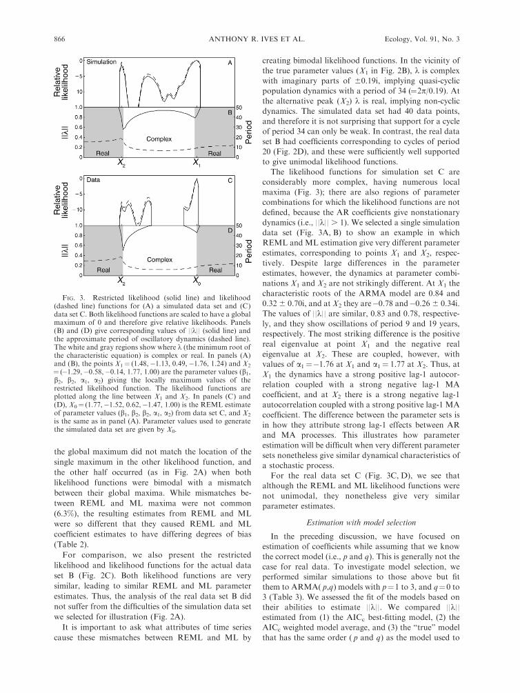
FIG. 3. Restricted likelihood (solid line) and likelihood(dashed line) functions for (A) a simulated data set and (C)data set C. Both likelihood functions are scaled to have a globalmaximum of 0 and therefore give relative likelihoods. Panels(B) and (D) give corresponding values of ||k|| (solid line) andthe approximate period of oscillatory dynamics (dashed line).The white and gray regions show where k (the minimum root ofthe characteristic equation) is complex or real. In panels (A)and (B), the points X1¼ (1.48,�1.13, 0.49,�1.76, 1.24) and X2

¼ (�1.29,�0.58,�0.14, 1.77, 1.00) are the parameter values (b1,b2, b2, a1, a2) giving the locally maximum values of therestricted likelihood function. The likelihood functions areplotted along the line between X1 and X2. In panels (C) and(D), X0¼ (1.77,�1.52, 0.62,�1.47, 1.00) is the REML estimateof parameter values (b1, b2, b2, a1, a2) from data set C, and X2

is the same as in panel (A). Parameter values used to generatethe simulated data set are given by X0.


simulate the data. Although researchers will not know

the true model for a given data set, we use the third

estimate of ||k|| to compare with the first two estimates

in order to assess the effects of uncertainty in model

selection on the estimates of ||k||.For simulation set A, AICc selected the true model

77% of the time, and the estimates of ||k|| from the best-

fitting model and from model averaging were similar to

those from the true model (with the correct p and q);

therefore, model selection added little bias to the

estimates of ||k||. In contrast, for simulation sets B and

C, model selection contributed downward bias to the

estimates of ||k|| when using both the best-fitting model

and model averaging. The proportion of simulations in

which the true model was selected was 29% and 26% for

simulation sets B and C, and the estimates of ||k|| for thebest-fitting model (B, 0.73; C, 0.69) and from model

averaging (B, 0.72; C, 0.70) were lower than those values

estimated using the true model (B, 0.78; C, 0.90). For

simulation set C in particular, the imprecision in the

estimates of ||k|| was increased due to model selection,

with 95% inclusion intervals for estimates from the best-

fitting model and model averaging of (0.08, 1.00) and

(0.31, 0.97), in comparison to (0.65, 1.00) from the fitted

true model.

To investigate the effects of measurement error, we

contaminated the simulation sets by setting m ¼ r as

above. We then performed model selection, first by

considering all models with p¼ 1 to 3 and q¼ 0 to 3, and

then by considering only those models with p¼ q¼ 1 to

3. The latter group of models implicitly incorporates

measurement error since measurement error will man-ifest as q ¼ p lags in the MA component of the model;

here, we assume that the underlying biological process

has order q � p, as is the case for our models used for

simulations. For simulation set A, model selection led to

less-biased estimates of ||k|| than those obtained from

the ‘‘true’’ ARMA(1,0) model; a greater fraction of

models was selected with q . 0 in the presence of

measurement error, and the MA components of these

models apparently absorbed some of the measurement

error. For models forced to have q ¼ p and thereby

conform to the stochastic process created by measure-

ment error, model selection added no bias to the

estimates of ||k|| (compare to Table 2, Simulation set

A). In contrast to simulation set A, model selection

failed to compensate well for measurement error for

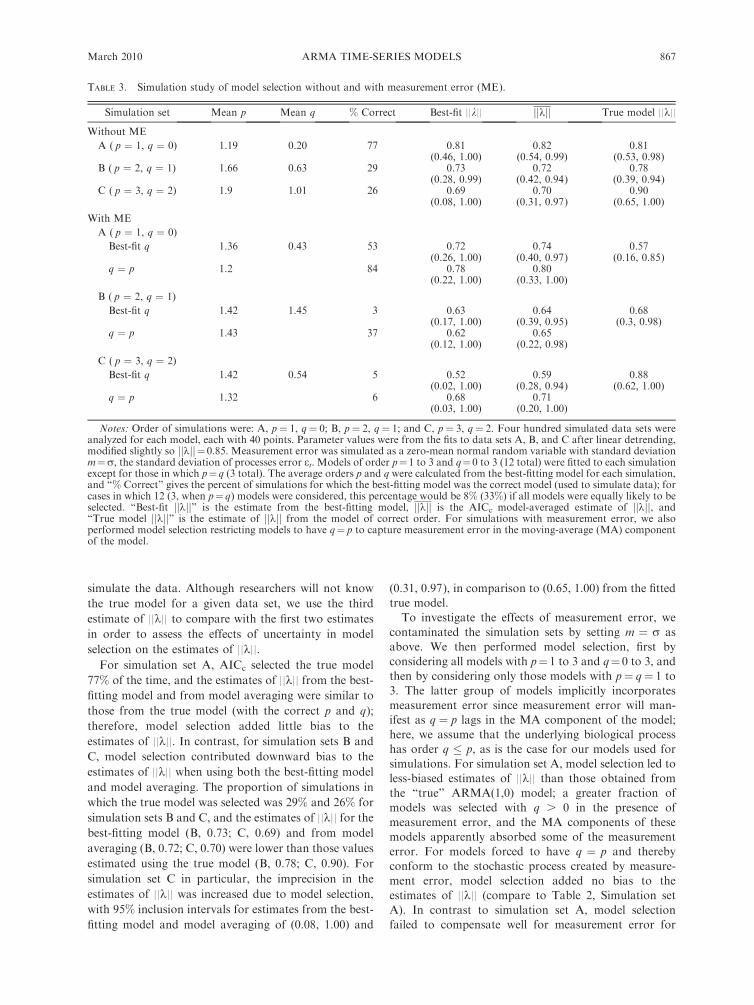
TABLE 3. Simulation study of model selection without and with measurement error (ME).

Simulation set Mean p Mean q % Correct Best-fit ||k|| jjkjj True model ||k||

Without ME

A ( p ¼ 1, q ¼ 0) 1.19 0.20 77 0.81 0.82 0.81(0.46, 1.00) (0.54, 0.99) (0.53, 0.98)

B ( p ¼ 2, q ¼ 1) 1.66 0.63 29 0.73 0.72 0.78(0.28, 0.99) (0.42, 0.94) (0.39, 0.94)

C ( p ¼ 3, q ¼ 2) 1.9 1.01 26 0.69 0.70 0.90(0.08, 1.00) (0.31, 0.97) (0.65, 1.00)

With ME

A ( p ¼ 1, q ¼ 0)

Best-fit q 1.36 0.43 53 0.72 0.74 0.57(0.26, 1.00) (0.40, 0.97) (0.16, 0.85)

q ¼ p 1.2 84 0.78 0.80(0.22, 1.00) (0.33, 1.00)

B ( p ¼ 2, q ¼ 1)

Best-fit q 1.42 1.45 3 0.63 0.64 0.68(0.17, 1.00) (0.39, 0.95) (0.3, 0.98)

q ¼ p 1.43 37 0.62 0.65(0.12, 1.00) (0.22, 0.98)

C ( p ¼ 3, q ¼ 2)

Best-fit q 1.42 0.54 5 0.52 0.59 0.88(0.02, 1.00) (0.28, 0.94) (0.62, 1.00)

q ¼ p 1.32 6 0.68 0.71(0.03, 1.00) (0.20, 1.00)

Notes: Order of simulations were: A, p¼ 1, q¼ 0; B, p¼ 2, q¼ 1; and C, p¼ 3, q¼ 2. Four hundred simulated data sets wereanalyzed for each model, each with 40 points. Parameter values were from the fits to data sets A, B, and C after linear detrending,modified slightly so jjkjj ¼0.85. Measurement error was simulated as a zero-mean normal random variable with standard deviationm¼r, the standard deviation of processes error et. Models of order p¼1 to 3 and q¼0 to 3 (12 total) were fitted to each simulationexcept for those in which p¼q (3 total). The average orders p and q were calculated from the best-fitting model for each simulation,and ‘‘% Correct’’ gives the percent of simulations for which the best-fitting model was the correct model (used to simulate data); forcases in which 12 (3, when p¼ q) models were considered, this percentage would be 8% (33%) if all models were equally likely to beselected. ‘‘Best-fit jjkjj’’ is the estimate from the best-fitting model, jjkjj is the AICc model-averaged estimate of jjkjj, and‘‘True model jjkjj’’ is the estimate of jjkjj from the model of correct order. For simulations with measurement error, we alsoperformed model selection restricting models to have q¼ p to capture measurement error in the moving-average (MA) componentof the model.


simulation set B, giving more severely downward biased

estimates of ||k|| than in the absence of measurement

error. Finally, for simulation set C, only limiting model

selection to ARMA( p,p) models provided some im-

provement in estimates of ||k||.

DISCUSSION

Time-series analyses of our three example data sets

using ARMA models were valuable, identifying con-

trasting dynamics among data sets and giving insight

into the contrasts. A single best-fitting structure for data

set A (Fig. 1A) could not be identified unequivocally;

models with AR lags of p¼ 1 and 3 were well-supported

(Table 1). Data set B (Fig. 1B) appeared to have either

an ARMA(2,0) or an ARMA(1,1) structure; there is a

lag structure to the data, although this could be either in

the AR component ( p ¼ 2) or MA component (q ¼ 1).

For data set C (Fig. 1C) all of the best models had p¼ 3,

indicating an AR structure with relatively long lags.

Even though these ARMA models are not mechanistic

and therefore give no detailed insight into the biological

processes generating the dynamics, they are nonetheless

useful for identifying contrasting patterns; they quantify

in a statistically rigorous fashion patterns that are visible

yet difficult to assuredly discern among data sets.

Despite these contrasts in lagged structures among

models fit to the data sets, all had values of ||k|| closer toone than zero. This implies that the dynamics were

weakly determined; populations are not brought rapidly

back to the mean of their stationary distribution

following a perturbation. The model averaged estimates

of ||k||, jjkjj, were 0.74, 0.63, and 0.92 for the non-

detrended data sets A, B, and C. When translated into

the half-life of a disturbance, the time required for the

expectation of the population density to traverse half the

distance to the mean of the stationary distribution, these

correspond to 2.3, 1.5, and 8.3 years, respectively.

A biologically important conclusion from these

analyses is that the populations have dynamics with

lagged structure. The study from which these data sets

were taken demonstrated a latitudinal gradient in the

cyclicity of grouse population dynamics, with popula-

tions at higher latitudes showing strong cyclicity and

populations at lower latitudes lacking cyclicity

(Williams et al. 2004). The three data sets we selected

were all from middle latitudes. Our present analyses

show strong cyclicity of period roughly 9 years for data

set C, and cyclicity of period 14–19 years for data set B;

if data set A is cyclic at all, the cycle period is longer

than 30 years. The lagged structure in the data sets

strongly suggests that there are underlying mechanisms

such as interactions with other species that are driving

the observed dynamics. The greater the number of lags,

the more key interacting species there are likely to be

(Royama 1992, Abbott et al. 2009). Our time-series

analyses, or any time-series analyses, cannot identify

what mechanisms generate the dynamics, but they do

demonstrate that something interesting underlies the

dynamics.

We have shown the need for caution when applying

standard estimation techniques for ARMA models. Our

simulations showed that the likelihood functions of

higher-order ARMAmodels applied to ‘‘short’’ data sets

(40 years) are likely to be multimodal. Dennis et al.

(2006: Fig. 3) showed that likelihood functions for

AR(1) models that simultaneously estimate process and

measurement error can be bimodal; this occurs as the

likelihood ‘‘trades off’’ process error against measure-

ment error. In our case, the likelihoods for dynamically

similar ARMA models are similar, and multimodality

arises as the lagged structure in the data is assigned to

either AR or MA components of the model.

Multimodality means that the naı̈ve application of

estimation techniques may lead to mistakes, identifying

PLATE 1. Greater Prairie Chicken female courted by, but ignoring, a booming male. Photo credit: Roger D. Applegate.


the incorrect parameter estimates that do not give the

global maximum of the likelihood function. Thus, there

is no substitute for investigating likelihood functions

themselves; this can be done using code such as we

provide in the Appendix. In addition to reducing

mistakes, this also can give useful information about

the data. For example, if the likelihood functions are

bimodal (Fig. 2A), comparing the parameter combina-

tions at the local maxima can identify what character-

istics of the dynamics (e.g., cyclicity) are supported with

high likelihoods (Fig. 2B).

Our main message is that any analysis with ARMA

models should include an investigation of the likelihood

functions. We have several additional recommendations

and observations. First, even though ML estimation

outperformed REML estimation for higher-order mod-

els, we nonetheless recommend using REML during

model selection because it performed better for our first-

order ( p ¼ 1) models; for low-order ARMA models,

REML generally has lower bias and higher precision

than ML estimation (McGilchrist 1989, Cheang and

Reinsel 2000, 2003, Kang et al. 2003). The better

performance we found for ML appeared to involve

cases with multimodal likelihood functions that do not

occur with low-order models. Given the better perfor-

mance of REML for simpler models, we feel it is

reasonable to apply REML in model selection when

there is no a priori knowledge of the complexity of the

dynamics of a data set. If REML identifies a higher-

order model, then ML estimation should be explored.

Our simulations showed that model selection often

contributed to downward bias in estimates of ||k||. Thisbias is distinct from the bias in ||k|| during parameter

estimation. The bias generated by model selection

implies that model selection favors models that describe

the data as being less dynamically active, with more

rapid characteristic return rates, than the stochastic

process generating the data. For higher-order stochastic

processes ( p � 2 and q � 1), AICc also tended to select

models of lower order (see also Abbott et al. 2009).

These results are not surprising since we investigated

relatively short data sets for which identifying the true

dynamical structure with longer lags might be expected

to be hard. In applying the methods we developed here

to 1583 time series of different lengths (Ziebarth et al.

2009), we found empirically that estimates of ||k|| withmodel selection increased continuously with the length

of the data set, with no apparent plateau for even the

longest data sets (.60).

As with other studies, we found that measurement

error contaminating data sets introduces bias for

parameter estimation and model selection (Shenk et al.

1998, Staudenmayer and Buonaccorsi 2005, Dennis

et al. 2006, Buonaccorsi and Staudenmayer 2009).

While measurement error can be explicitly incorporated

into models for estimation (Bell and Wilcox 1993,

Staudenmayer and Buonaccorsi 2005), we found that

using the simpler approach of fitting ARMA( p,p)

models worked reasonably well to estimate the AR

coefficients of the model with little excess bias. This

works because measurement errors in an ARMA( p,q,p)

model will produce non-zero MA coefficients of order up

to p. Of course, this approach does not help to estimate

the true (uncontaminated) MA coefficients of the model.

Nonetheless, questions regarding the dynamical charac-

teristics of a stochastic process center on AR coefficients,

so estimates of AR coefficients may be sufficient. While

the approach of fitting only ARMA( p,p) models might

reduce the bias in estimates of AR coefficients and ||k||,measurement error may nonetheless decrease the preci-

sion of the estimates, leading to estimates with higher

uncertainty (Staudenmayer and Buonaccorsi 2005).

Using ARMA( p,p) models to implicitly account for

measurement error brings up the question of whether

only ARMA( p,p) models should be considered during

model selection, or whether model selection should be

used to select the MA lag order (q). In our simulation

study (Table 3), we found that confining the selection to

ARMA( p,p) models could perform better than selec-

tion over all models when we knew measurement error

was present. Nonetheless, these simulations involved

large amounts of measurement error (m ¼ r). With

smaller amounts of measurement error, or when the

true MA dimension exceeds p, restricting selection to

ARMA( p,p) models may be too limiting. Overall,

measurement error presented a serious challenge during

model selection when the process generating data was

higher order ( p � 2), with the resulting estimates of ||k||considerably biased.

In summary, fitting ARMAmodels to time-series data

will likely give valuable information about the structure

of the stochastic process generating the data. ARMA

models can also be used to compare data sets; model

selection and estimation can be automated, making it

possible to submit a large number of data sets to the

same analyses and using this to compare, for example,

the characteristic return time (||k||) among them. Fitting

ARMA models needs to be done cautiously, however.

We have outlined many of the challenges of fitting

ARMA models. Simulations (not presented) showed

that these challenges largely evaporate for data sets with

250 or more points. Unfortunately, many ecological

time series do not offer the luxury of such length, so

ecologists are stuck with facing these difficult, but not

insurmountable, challenges.

ACKNOWLEDGMENTS

We thank C. K. Williams for providing the example datasets. This work was funded in part by NSF grants DEB-0411760, EF-0434329, and DEB 0816613 to A. R. Ives.

LITERATURE CITED

Abbott, K. C., J. Ripa, and A. R. Ives. 2009. Environmentalvariation in ecological communities and inferences fromsingle-species data. Ecology 90:1268–1278.

Bell, W. R., and D. W. Wilcox. 1993. The effects of samplingerror on the time-series behavior of consumption data.Journal of Econometrics 55:235–265.


Biggs, R., S. R. Carpenter, and W. A. Brock. 2009. Turningback from the brink: detecting an impending regime shift intime to avert it. Proceedings of the National Academy ofSciences (USA) 106:826–831.

Bjornstad, O. N., and B. T. Grenfell. 2001. Noisy clockwork:time series analysis of population fluctuations in animals.Science 293:638–643.

Box, G. E. P., G. M. Jenkins, and G. C. Reinsel. 1994. Timeseries analysis: forecasting and control. Third edition.Prentice Hall, Englewood Cliffs, New Jersey, USA.

Brook, B. W., and C. J. A. Bradshaw. 2006. Strength ofevidence for density dependence in abundance time series of1198 species. Ecology 87:1445–1451.

Buonaccorsi, J. P., and J. Staudenmayer. 2009. Statisticalmethods to correct for observation error in a density-independent population model. Ecological Monographs 79:299–324.

Burnham, K. T., and D. R. Anderson. 2002. Model selectionand inference: a practical information-theoretic approach.Second edition. Springer, New York, New York, USA.

Cheang, W. K., and G. C. Reinsel. 2000. Bias reduction ofautoregressive estimates in time series regression modelthrough restricted maximum likelihood. Journal of theAmerican Statistical Association 95:1173–1184.

Cheang, W. K., and G. C. Reinsel. 2003. Finite sampleproperties of ML and REML estimators in time seriesregression models with long memory noise. Journal ofStatistical Computation and Simulation 73:233–259.

Coulson, T., E. A. Catchpole, S. D. Albon, B. J. T. Morgan,J. M. Pemberton, T. H. Clutton-Brock, M. J. Crawley, andB. T. Grenfell. 2001. Age, sex, density, winter weather, andpopulation crashes in Soay sheep. Science 292:1528–1531.

Dennis, B., R. A. Desharnais, J. M. Cushing, S. M. Henson,and R. F. Costantino. 2001. Estimating chaos and complexdynamics in an insect population. Ecological Monographs71:277–303.

Dennis, B., P. L. Munholland, and J. M. Scott. 1991.Estimation of growth and extinction parameters for endan-gered species. Ecological Monographs 61:115–143.

Dennis, B., J. M. Ponciano, S. R. Lele, M. L. Taper, and D. F.Staples. 2006. Estimating density dependence, process noise,and observation error. Ecological Monographs 76:323–341.

Dennis, B., and B. Taper. 1994. Density dependence in timeseries observations of natural populations: estimation andtesting. Ecological Monographs 64:205–224.

de Valpine, P., and A. Hastings. 2002. Fitting populationmodels incorporating process noise and observation error.Ecological Monographs 72:57–76.

Ellner, S., and P. Turchin. 1995. Chaos in a ‘‘noisy’’ world: newmethods and evidence from time series analysis. AmericanNaturalist 145:343–375.

Fagan, W. F. 2001. Characterizing population vulnerability for758 species. Ecology Letters 4:132–138.

Fromentin, J. M., R. A. Myers, O. N. Bjornstad, N. C.Stenseth, J. Gjosaeter, and H. Christie. 2001. Effects ofdensity-dependent and stochastic processes on the regulationof cod populations. Ecology 82:567–579.

Fuller, W. A. 1996. Introduction to statistical time series.Second edition. John Wiley and Sons, New York, New York,USA.

Galeano, P., and D. Pena. 2007. On the connection betweenmodel selection criteria and quadratic discrimination inARMA time series models. Statistics and ProbabilityLetters 77:896–900.

Gross, K., A. R. Ives, and E. V. Nordheim. 2005. Estimatingtime-varying vital rates from observation time series: a casestudy in aphid biological control. Ecology 86:740–752.

Hauser, M. A. 1999. Maximum likelihood estimators forARMA and ARFIMA models: a Monte Carlo study.Journal of Statistical Planning and Inference 80:229–255.

Hilborn, R., and M. Mangel. 1997. The ecological detective:confronting models with data. Princeton University Press,Princeton, New Jersey, USA.

Hurvich, C. M., and C. L. Tsai. 1989. Regression and time-series models selection in small samples. Biometrika 76:297–307.

Ives, A. R., B. Dennis, K. L. Cottingham, and S. R. Carpenter.2003. Estimating community stability and ecological inter-actions from time-series data. Ecological Monographs 73:301–330.

Ives, A. R., A. Einarsson, V. A. A. Jansen, and A. Gardarsson.2008. High-amplitude fluctuations and alternative dynamicalstates of midges in Lake Myvatn. Nature 452:84–87.

Kang, W. C., D. W. Shin, and Y. Lee. 2003. Biases of therestricted maximum likelihood estimators for ARMA pro-cesses with polynomial time trend. Journal of StatisticalPlanning and Inference 116:163–176.

Kendall, B. E., C. J. Briggs, W. W. Murdoch, P. Turchin, S. P.Ellner, E. McCauley, R. M. Nisbet, and S. N. Wood. 1999.Why do populations cycle? A synthesis of statistical andmechanistic modeling approaches. Ecology 80:1789–1805.

Kendall, M. G. 1954. A note on the bias in the estimation of anautocorrelation. Biometrika 41:403–404.

Kirkpatrick, S., C. D. Gelatt, and M. P. Vecchi. 1983.Optimization by simulated annealing. Science 220:671–680.

Knape, J. 2008. Estimatibility of density dependence in modelsof time series data. Ecology 89:2994–3000.

Lande, R. 2002. Estimating density dependence in time-series ofage-structured populations. Philosophical Transactions ofthe Royal Society B 357:1179–1184.

Liang, G., D. M. Wilkes, and J. A. Cadzow. 1993. ARMAmodel order estimation based on the eigenvalues of thecovariance matrix. LEEE Transactions on Signal Processing41:3003–3009.

Malgras, J., and D. Debouzie. 1997. Can ARMA models beused reliably in ecology? Acta Oecologica InternationalJournal of Ecology 18:427–447.

MathWorks. 2005. MATLAB. The MathWorks, Inc., Natick,Massachusetts, USA.

McGilchrist, C. A. 1989. Bias of ML and REML estimators inregression models with ARMA errors. Journal of StatisticalComputation and Simulation 32:127–136.

Morris, W. F., and D. F. Doak. 2002. Quantitative conserva-tion biology: theory and practice of population viabilityanalysis. Sinauer Associates, Sunderland, Massachusetts,USA.

Mullon, C., P. Freon, and P. Cury. 2005. The dynamics ofcollapse in world fisheries. Fish and Fisheries 6:111–120.

Murdoch, W. W., B. E. Kendall, R. M. Nisbet, C. J. Briggs, E.McCauley, and R. Bolser. 2002. Single-species models formany-species food webs. Nature 417:541–543.

Potscher, B. M., and S. Srinivasan. 1994. A comparison oforder estimation procedures for ARMA models. StatisticaSinica 4:29–50.

Quenouille, M. H. 1949. Approximate tests of correlation intime series. Journal of the Royal Statistical Society, Series B11:68–83.

R Development Core Team. 2008. R: a language andenvironment for statistical computing. R Foundation forStatistical Computing, Vienna, Austria.

Royama, T. 1992. Analytical population dynamics. Chapmanand Hall, London, UK.

Sæther, B.-E., et al. 2005. Generation time and temporal scalingof bird population dynamics. Nature 436:99–102.

Scheffer, M., and S. R. Carpenter. 2003. Catastrophic regimeshifts in ecosystems: linking theory to observation. Trends inEcology and Evolution 18:648–656.

Shenk, T. M., G. C. White, and K. P. Burnham. 1998. Samplingvariance effects on detecting density dependence fromtemporal trends in natural populations. EcologicalMonographs 68:445–463.


Shibata, R. 1976. Selection of order of an autoregressive modelby Akaikes information criterion. Biometrika 63:117–126.

Sibly, R. M., D. Barker, J. Hone, and M. Pagel. 2007. On thestability of populations of mammals, birds, fish and insects.Ecology Letters 10:970–976.

Staples, D. F. 2004. Estimating population trend and processvariation for PVA in the presence of sampling error. Ecology85:923–929.

Stark, J. 1999. Delay embeddings for forced systems. I.Deterministic forcing. Journal of Nonlinear Science 9:255–332.

Stark, J., D. S. Broomhead, M. E. Davies, and J. Huke. 2003.Delay embeddings for forced systems. II. Stochastic forcing.Journal of Nonlinear Science 13:519–577.

Staudenmayer, J., and J. R. Buonaccorsi. 2005. Measurementerror in linear autoregressive models. Journal of theAmerican Statistical Association 100:841–852.

Takens, F. 1981. Detecting strange attractors in turbulence.Pages 366–381 in D. A. Rand and L. S. Young, editors.Dynamical systems and turbulence. Springer-Verlag, NewYork, New York, USA.

Tsimikas, J., and J. Ledolter. 1994. REML and best linearunbiased prediction in state-space models. Communicationsin Statistics: Theory and Methods 23:2253–2268.

Tsimikas, J. V., and J. Ledolter. 1998. Analysis of multi-unitvariance components models with state space profiles. Annalsof the Institute of Statistical Mathematics 50:147–164.

Turchin, P. 1990. Rarity of density dependence or populationregulation with lags? Nature 344:660–663.

Turchin, P., and A. D. Taylor. 1992. Complex dynamics inecological time series. Ecology 73:289–305.

Williams, C. K., A. R. Ives, R. D. Applegate, and J. Ripa. 2004.The collapse of cycles in the dynamics of North Americangrouse populations. Ecology Letters 7:1135–1142.

Wold, H. 1938. A study in the analysis of stationary time series.Almqvist and Wiksells, Uppsala, Sweden.

Zeng, Z., R. M. Nowierski, M. L. Taper, B. Dennis, and W. P.Kemp. 1998. Complex population dynamics in the realworld: modeling the influence of time-varying parametersand time lags. Ecology 79:2193–2209.

Ziebarth, N. L., K. C. Abbott, and A. R. Ives. 2009. Weakpopulation regulation in ecological time series. EcologyLetters, in press.

APPENDIX

Descriptions of the derivation of likelihood and restricted likelihood functions for an ARMA( p,q) process, including theincorporation of measurement error (Ecological Archives E091-062-A1).

SUPPLEMENT

MATLAB and R code for performing ARMA( p,q) model fitting (Ecological Archives E091-062-S1).


Documents

Analysis of ecological time series with ARMA( ) modelscase.edu/artsci/biol/abbottlab/Things_files/Ives,Abbott... · Analysis of ecological time series with ARMA(p,q) models ... Corresponding