Analysis of 3D Cone-Beam CT Image Reconstruction

Western University Western University

Scholarship@Western Scholarship@Western

Electronic Thesis and Dissertation Repository

12-16-2016 12:00 AM

Analysis of 3D Cone-Beam CT Image Reconstruction Analysis of 3D Cone-Beam CT Image Reconstruction

Performance on a FPGA Performance on a FPGA

Devin Held, The University of Western Ontario

Supervisor: Michael Bauer, The University of Western Ontario

A thesis submitted in partial fulfillment of the requirements for the Master of Science degree in

Computer Science

© Devin Held 2016

Follow this and additional works at: https://ir.lib.uwo.ca/etd

Part of the Hardware Systems Commons, Software Engineering Commons, and the Theory and

Algorithms Commons

Recommended Citation Recommended Citation Held, Devin, "Analysis of 3D Cone-Beam CT Image Reconstruction Performance on a FPGA" (2016). Electronic Thesis and Dissertation Repository. 4349. https://ir.lib.uwo.ca/etd/4349

This Dissertation/Thesis is brought to you for free and open access by Scholarship@Western. It has been accepted for inclusion in Electronic Thesis and Dissertation Repository by an authorized administrator of Scholarship@Western. For more information, please contact [email protected].

https://ir.lib.uwo.ca/

https://ir.lib.uwo.ca/etd

https://ir.lib.uwo.ca/etd?utm_source=ir.lib.uwo.ca%2Fetd%2F4349&utm_medium=PDF&utm_campaign=PDFCoverPages

http://network.bepress.com/hgg/discipline/263?utm_source=ir.lib.uwo.ca%2Fetd%2F4349&utm_medium=PDF&utm_campaign=PDFCoverPages




https://ir.lib.uwo.ca/etd/4349?utm_source=ir.lib.uwo.ca%2Fetd%2F4349&utm_medium=PDF&utm_campaign=PDFCoverPages

mailto:[email protected]

Held, Devin i

Abstract Efficient and accurate tomographic image reconstruction has been an intensive topic of research

due to the increasing everyday usage in areas such as radiology, biology, and materials science.

Computed tomography (CT) scans are used to analyze internal structures through capture of x-

ray images. Cone-beam CT scans project a cone-shaped x-ray to capture 2D image data from a

single focal point, rotating around the object. CT scans are prone to multiple artifacts, including

motion blur, streaks, and pixel irregularities, therefore must be run through image reconstruction

software to reduce visual artifacts. The most common algorithm used is the Feldkamp, Davis,

and Kress (FDK) backprojection algorithm. The algorithm is computationally intensive due to

the O(n4) backprojection step, running slowly with large CT data files on CPUs, but

exceptionally well on GPUs due to the parallel nature of the algorithm. This thesis will analyze

the performance of 3D cone-beam CT image reconstruction implemented in OpenCL on a FPGA

embedded into a Power System.

Keywords Image reconstruction, image processing, FPGA, Power8, cone-beam CT, GPU

Held, Devin ii

Acknowledgments I would like to thank my supervisor, Michael Bauer, for his guidance on my thesis and

throughout my master’s degree. I would also like to acknowledge Sean Wagner and James Ooi

from IBM for setting up the necessary hardware required and their assistance and

troubleshooting help with the Altera OpenCL SDK and FPGAs.

Held, Devin iii

Table of Contents

Abstract ............................................................................................................................................ i

Keywords ......................................................................................................................................... i

Acknowledgments........................................................................................................................... ii

Table of Contents ........................................................................................................................... iii

List of Figures ................................................................................................................................. v

List of Tables ................................................................................................................................ vii

1 Introduction .................................................................................................................................. 1

1.1: Tomography Overview ....................................................................................................... 1

1.2: CT Scans ............................................................................................................................. 2

1.2.1: X-Rays ........................................................................................................................ 3

1.2.2: Fan-Beam Computed Tomography ............................................................................ 5

1.2.3: Cone-Beam Computed Tomography .......................................................................... 6

1.2.4: Image Reconstruction Overview ................................................................................ 7

1.3: Explorations ........................................................................................................................ 9

1.4: Summary and Thesis Overview ........................................................................................ 10

2 3D CT Image Reconstruction .................................................................................................... 11

2.1: Fourier Transform ............................................................................................................. 11

2.2: Ramp Filtering .................................................................................................................. 12

2.3: Fan Beam CT Image Reconstruction ................................................................................ 15

2.3.1: Algorithm and Mathematical Analysis ..................................................................... 16

2.4: Cone Beam CT Image Reconstruction ............................................................................. 18

2.4.1: Reconstruction Process ............................................................................................. 18

2.4.2: Tuy’s Condition ........................................................................................................ 20

2.4.3: Grangeat’s Algorithm ............................................................................................... 20

2.4.4: Katsevich’s Algorithm .............................................................................................. 22

2.5: Feldkamp, Davis and Kress Algorithm............................................................................. 23

2.5.1: Algorithm and Mathematical Analysis ..................................................................... 24

2.6: Performance Bottlenecks .................................................................................................. 27

3 Related Work ............................................................................................................................. 29

Held, Devin iv

3.1: Related Work 1 - “Accelerated cone-beam CT reconstruction based on OpenCL” by

Wang et al. [18]............................................................................................................................. 29

3.1.1: Implementation ......................................................................................................... 30

3.1.2: Conclusions ............................................................................................................... 30

3.2: Related Work 2 - “GPU-based cone beam computer tomography” by Noel et al. [17] ... 31

3.2.1: Implementation ......................................................................................................... 31

3.2.2: Conclusions ............................................................................................................... 32

3.3: Related Work 3 - “High-Performance Cone Beam Reconstruction Using CUDA

Compatible GPUs” by Okitsu et al. [16] ...................................................................................... 32

3.3.1: Implementation ......................................................................................................... 32

3.3.2: Conclusions ............................................................................................................... 33

3.4: Related Work 4 - “High speed 3D tomography on CPU, GPU, and FPGA” Gac et al….34

3.4.1: Implementation ......................................................................................................... 34

3.4.2: Conclusions ............................................................................................................... 35

3.5: Summary and Thesis Direction......................................................................................... 36

4 FPGAs and Power8 .................................................................................................................... 37

4.1: Field Programmable Gate Arrays (FPGAs) ...................................................................... 37

4.1.1: Architecture .............................................................................................................. 39

4.1.2: Development Process ................................................................................................ 40

4.1.3: Comparison with GPU and ASICS ........................................................................... 40

4.2 Power8 Technology ........................................................................................................... 41

4.3: FPGA and Power8 Configuration ..................................................................................... 42

4.3.1: Nallatech Card with Altera Stratix V FPGA ............................................................ 43

4.3.2:IBM Power System S822L ........................................................................................ 43

5 Benchmarking and Results ........................................................................................................ 44

5.1: OpenCL ............................................................................................................................. 45

5.1.1: Altera SDK for OpenCL ........................................................................................... 45

5.2: Implementation ................................................................................................................. 46

5.3: Benchmarking ................................................................................................................... 48

5.3.1: Test Beds................................................................................................................... 48

5.3.2: Test Data ................................................................................................................... 49

Held, Devin v

5.3.3: Experimental Results ................................................................................................ 50

5.4: Observations ........................................................................................................ 51

5.5: Power Usage Analysis ...................................................................................................... 57

6 Conclusions and Future Directions ............................................................................................ 59

6.1: Conclusions ....................................................................................................................... 60

6.2: Future Directions .............................................................................................................. 61

References ..................................................................................................................................... 63

Curriculum Vitae………………………………………………………………………………...66

List of Figures

Held, Devin vi

Figure 1: CT Scan of Human Brain (innerbody.com)

Figure 2: Fan-Beam and Cone-Beam Projections (J. Can Dental Association)

Figure 3: Fan-Beam CT System (www.mathworks.com)

Figure 4: Cone-Beam CT System (opticalengineering.spiedigitallibrary.org)

Figure 5: Fourier Transform Equations (Credit: roymech.co.uk)

Figure 6: (a) Original image, (b) unfiltered back projected image, and (c) ramp filtered image.

(Credit: www.clear.rice.edu)

Figure 7: Fan-Beam computed tomography (Credit: Journal of Nuclear Medicine and

Technology)

Figure 8: Fan-beam coordinate system (Credit: Zeng et al. [20])

Figure 9: Steps in the reconstruction process (Credit: Scarfe et al. [13])

Figure 10: Fan-Beam Reconstruction Formula (Credit: Zeng et al. [20])

Figure 11: Tuy’s Condition (Credit: Zeng et al. [20])

Figure 12: Grangeat’s Algorithm Visual Aid (Credit: Zeng et al. [20])

Figure 13: Helical orbit used in Katsevich’s Algorithm (Credit: Zeng et al. [20])

Figure 14: Feldkamp Algorithm Visual (Credit: Zeng et al. [20])

Figure 15: Cone-Beam Coordinate System (Credit: Zeng et al. [20])

Figure 16: FDK Reconstruction Algorithm (Credit: Zeng et al. [20])

Figure 17: Volume Data Subrow Parallization (Credit: Noel et al. [17])

Figure 18: Proposed Optimization Method on GPUs (Okitsu et. al [16])

Figure 19: FPGA Evaluation System (Credit: Gac et al. [19])

Figure 20: Altera Stratix V Chip (Credit: Altera)

Figure 21: Block Diagram of FPGA Board (Credit: rfwireless-world.com)

Figure 22: Power8 Specs (Credit: IBM)

Figure 23: Altera SDK for OpenCL Proces (Credit: altera.com)

Figure 24: Shepp Logan Phantom (Generated from MatLab)

Figure 25: CPU vs. GPU 2563 Phantom Image Run Times

Figure 26: CPU vs. GPU 5123 Phantom Image Run Times

Figure 27: CPU vs. FPGA 2563 Phantom Image Run Times

Figure 28: CPU vs. FPGA 5123 Phantom Image Run Times

Figure 29: GPU vs. FPGA 2563 Phantom Image Run Times

http://innerbody.com/

http://www.mathworks.com/

http://opticalengineering.spiedigitallibrary.org/

http://roymech.co.uk/

http://www.clear.rice.edu/

http://rfwireless-world.com/

http://altera.com/

Held, Devin vii

Figure 30: GPU vs. FPGA 5123 Phantom Image Run Times

Figure 31: CPU vs. GPU vs. FPGA 2563 Phantom Image Run Times

Figure 32: CPU vs. GPU vs. FPGA 5123 Phantom Image Run Times

List of Tables

Held, Devin viii

Table 1: Description of General 2D Image Reconstruction

Table 2: Description of Feldkamp et al. Algorithm

Table 3: Implementation Pseudo Code

Table 4: Test Bed Specifications

Table 5: Watts per Device

Table 6: Estimated Energy Usage

Held, Devin 1

Chapter 1

1 Introduction

Efficient and accurate tomographic image reconstruction has been an intensive topic of

research due to its increasing everyday use in areas such as radiology, biology, and materials

science. The capture of tomographic images allows specialists to feed CT image data through a

software application, run computationally intensive image processing algorithms on the images,

and reconstruct a three dimensional image with reduced pixel irregularities. This is frequently

used in medical areas through the use of x-ray computed tomography (CT) scans in order to

analyze specific internal structures and to provide more informative views of internal areas of

interest.

CT scanners record x-ray image data through a variety of approaches including fan-beam

and cone-beam computed tomography, providing different techniques to section image slices.

Details of both tomography types are described in subsequent sections. By far, the most

computationally intensive task is reconstructing the image slices. It not only takes quite a bit of

time to run the specific algorithms, but it requires a powerful machine to execute the operations.

Such operations are time consuming on the central processing unit (CPU) of a computer, thus

implementations on accelerators such as a graphics processing unit (GPU) or a field-

programmable gate array (FPGA) are popular areas of research for these types of tasks.

Accelerators have the ability of reducing the run time of operations because they essentially

offload a lot of the computations from the CPU to the accelerator themselves.

Through tomographic images and image processing software, computed tomography is

able to provide specialists with detailed information regarding an area of interest and assist in

identifying underlying medical problems unclear in a single x-ray image. There are medical

scenarios where time is of the essence, and researching more efficient ways to run the image

reconstruction on sets of CT image slices deems itself an important area of research.

1.1: Tomography Overview

Tomography, directly meaning “slice imaging”, involves the capture of two dimensional

images in sections through movement of the camera source around a three dimensional object.

Held, Devin 2

These sectioned images are called projections, and are fed through specific image reconstruction

applications to process the final image. Tomographic images are essential in medical and non-

destructive testing scenarios because they capture accurate and informative views of both the

internal human body and other objects.

Classical tomography has quite the interesting history, as it has been claimed that ten

people independently invented tomography over a ten year period beginning in 1921 [5]. None

of those ten people had any idea what the other nine were doing during those times, and when it

was discovered that they all had in fact invented the same things, there were arguments about

who invented and patented the idea first, which lead to the news of the invention reaching

worldwide awareness [5]. After many disputes regarding the issue, people are lead to believe that

the fundamental beginnings to the invention of tomography was indirectly invented in 1914 by

Karol Mayer, who used camera motion to sharpen and blur parts of the images based on distance

from the focal point [5,6].

Today, tomography involves taking many images from different angles in regards to a

focal point. Types of tomographic images, called tomograms, include hydraulic tomography,

magnetic particle imaging, and CT scans. These tomograms provide informative views to

diagnose problems within the area of interest. The use of tomograms is diverse across many

areas of study, and is therefore an important technology in modern society.

1.2: CT Scans

After the first computed tomography (CT) scanner was released in 1971, it was quickly

described as the “greatest diagnostic discovery since x-rays themselves in 1895” [5]. A CT scan

is an essential tool used to produce informative three dimensional images internal views of an

object, most commonly used in medical applications to study specific parts of the body. They

can be used to diagnose particular injuries, diseases, tumours, and many other problems within

the body. In 2012, the Canadian Institute for Health Information released data that concluded 4.4

million CT scans were performed in Canada alone on the available 510 CT Scanners,

dramatically increasing in usage from previous decades [1]. The high usage volumes in Canada

alone are means for exploring more effective ways to analyze CT images.

Held, Devin 3

Patients typically undress and put on a hospital gown before scan. They are also typically

instructed to fast before for some time before the scan. At the time of the scan, the patient will

lay on a flat table attached to the CT scanner and may be given a “contrast material” introduced

to the body through a vein or a joint in order to highlight certain areas better under the CT

scanner. The patient must lay very still within the CT scanner to avoid noise and error within the

images taken. Each image takes half a second to acquire [4] as the scanner rotates and takes

tomographic slice images through the use of x-rays.

1.2.1: X-Rays

CT scans use x-ray images to generate the tomographic slice images. X-rays are a type of

electromagnetic radiation with higher energy than visible light and therefore have the ability to

travel through various types objects to provide a means of “seeing” the internal structures. In

medical applications, x-rays pass through our bodies, allowing film to capture projections of

internal structures. This is due to tissues and organs absorbing varying levels of the x-rays,

depending on the radiological density, as determined by material density and also the number on

the atomic scale. [2] X-rays produce a clear visual of bone structures, but are two dimensional

and therefore much information is lost in the image. CT scans minimize this information loss

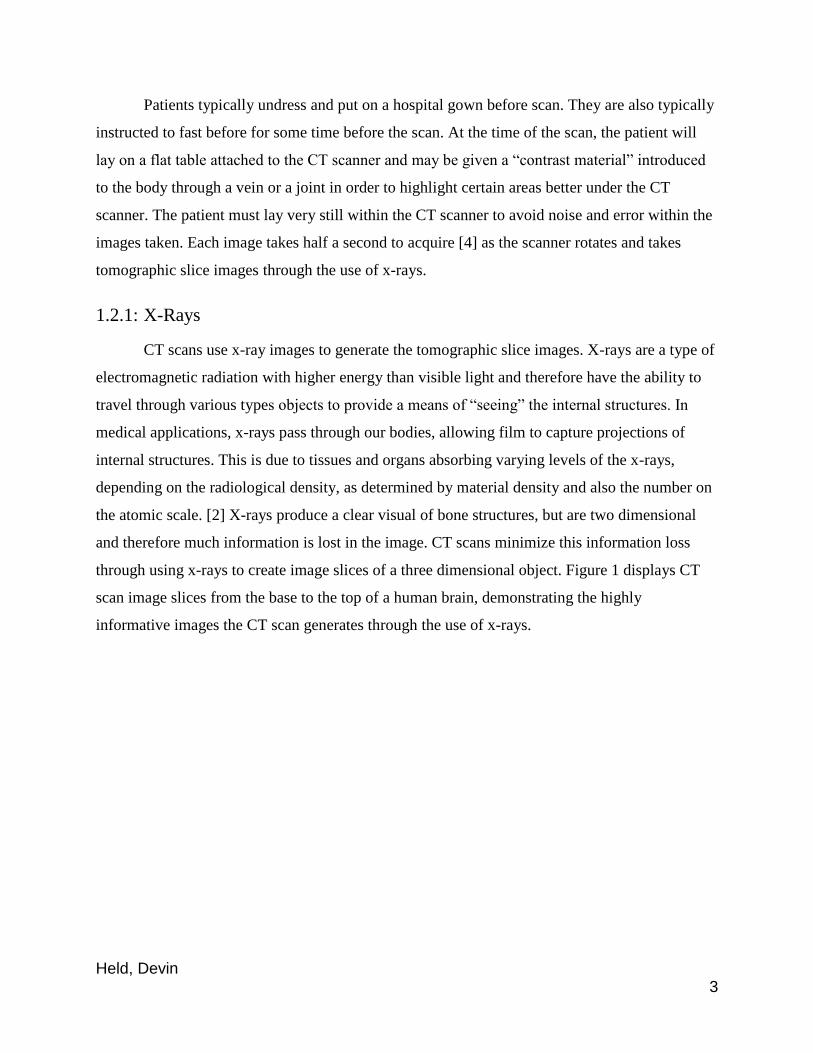
through using x-rays to create image slices of a three dimensional object. Figure 1 displays CT

scan image slices from the base to the top of a human brain, demonstrating the highly

informative images the CT scan generates through the use of x-rays.

Held, Devin 4

Figure 1 (Credit: innerbody.com)

In CT scans, x-rays are not stationary. The x-rays are rotated about an axis, continuously

gathering information about a patient’s body through a certain focal point. This data is run

through a software program in order to create two dimensional slice images, which can later be

combined to create the three dimensional image representation; the software enables certain

filtering operations to be run on the images.

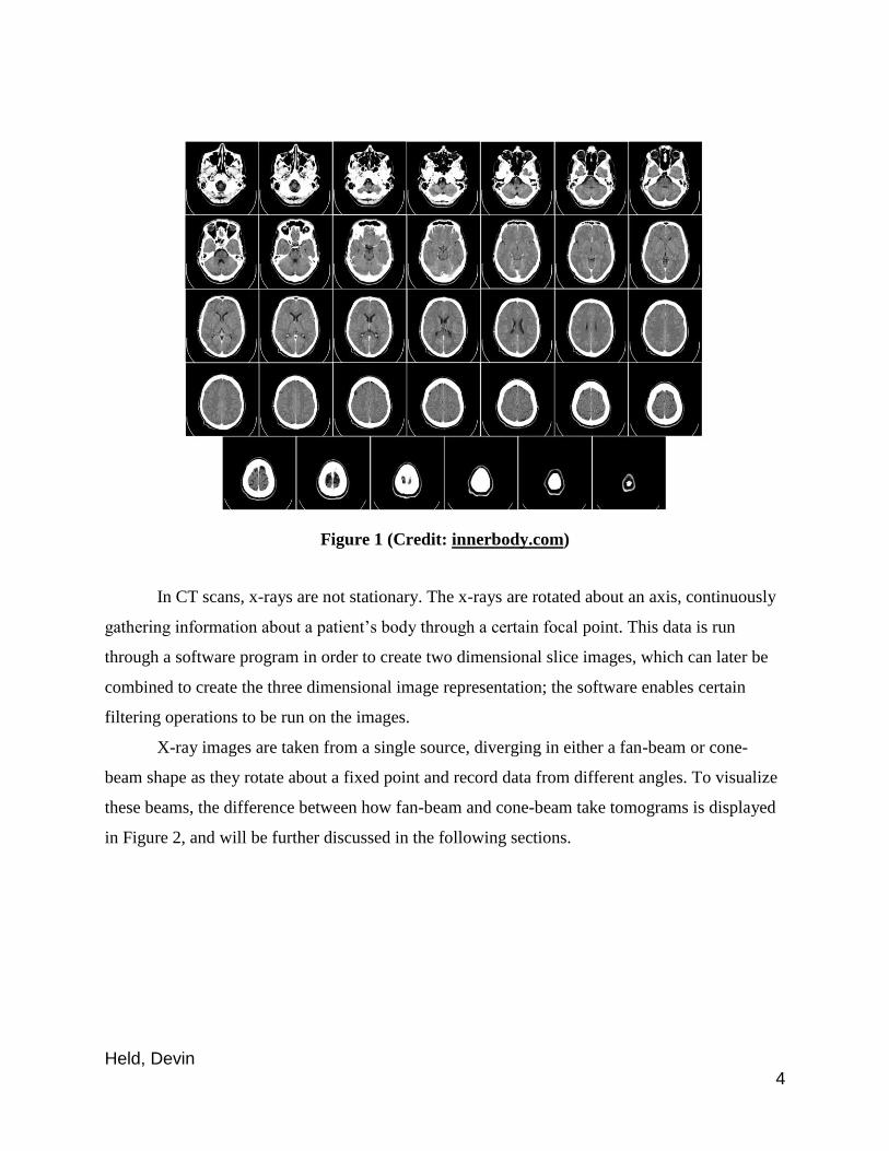
X-ray images are taken from a single source, diverging in either a fan-beam or cone-

beam shape as they rotate about a fixed point and record data from different angles. To visualize

these beams, the difference between how fan-beam and cone-beam take tomograms is displayed

in Figure 2, and will be further discussed in the following sections.

http://innerbody.com/

Held, Devin 5

Figure 2 (Credit: J. Can Dental Association).

Once a single x-ray image is taken at a specific angle, the data is sent to the specialist’s

computer in order to run reconstruction algorithms to essentially improve the image quality and

recreate the two or three dimensional images, as described in detail in Chapter 2. After all images

are successfully taken, the radiologist must wait for the computationally intensive reconstruction

process to complete before analyzing the results from the CT scan. Depending on the number of

image slices, image quality, and hardware used to reconstruct the images, this process has

potential to take a long time to fully compute.

1.2.2: Fan-Beam Computed Tomography

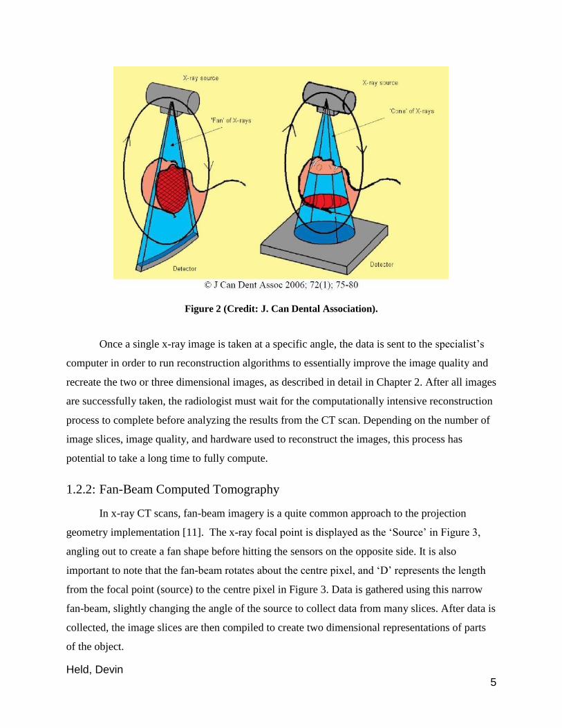
In x-ray CT scans, fan-beam imagery is a quite common approach to the projection

geometry implementation [11]. The x-ray focal point is displayed as the ‘Source’ in Figure 3,

angling out to create a fan shape before hitting the sensors on the opposite side. It is also

important to note that the fan-beam rotates about the centre pixel, and ‘D’ represents the length

from the focal point (source) to the centre pixel in Figure 3. Data is gathered using this narrow

fan-beam, slightly changing the angle of the source to collect data from many slices. After data is

collected, the image slices are then compiled to create two dimensional representations of parts

of the object.

Held, Devin 6

Figure 3: Fan-Beam CT System (Credit: www.mathworks.com)

A disadvantage of fan-beam imaging is that part of the image data may be truncated due

to the limited field of view from the magnification factor, causing spikes and other artifacts

around the edges of the image. [10].

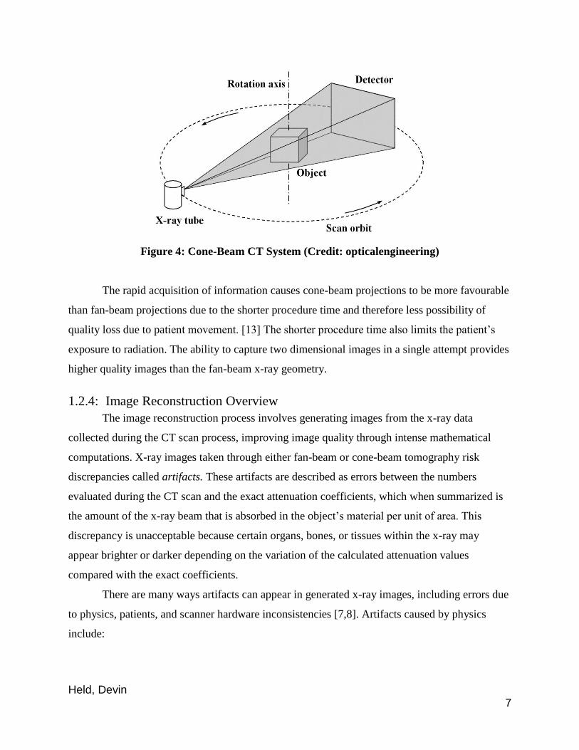
1.2.3: Cone-Beam Computed Tomography

Unlike the thin fan-beam geometry, cone-beam geometry immediately captures a two

dimensional image through a three dimensional x-ray beam, which scans in the shape of a cone.

The x-ray tube and detector rotate about the object of interest, as displayed in Figure 4. This

three dimensional beam proves efficient as at most one rotation around the object provides

enough information to reconstruct a three dimensional image. [12]

http://www.mathworks.com/

Held, Devin 7

Figure 4: Cone-Beam CT System (Credit: opticalengineering)

The rapid acquisition of information causes cone-beam projections to be more favourable

than fan-beam projections due to the shorter procedure time and therefore less possibility of

quality loss due to patient movement. [13] The shorter procedure time also limits the patient’s

exposure to radiation. The ability to capture two dimensional images in a single attempt provides

higher quality images than the fan-beam x-ray geometry.

1.2.4: Image Reconstruction Overview

The image reconstruction process involves generating images from the x-ray data

collected during the CT scan process, improving image quality through intense mathematical

computations. X-ray images taken through either fan-beam or cone-beam tomography risk

discrepancies called artifacts. These artifacts are described as errors between the numbers

evaluated during the CT scan and the exact attenuation coefficients, which when summarized is

the amount of the x-ray beam that is absorbed in the object’s material per unit of area. This

discrepancy is unacceptable because certain organs, bones, or tissues within the x-ray may

appear brighter or darker depending on the variation of the calculated attenuation values

compared with the exact coefficients.

There are many ways artifacts can appear in generated x-ray images, including errors due

to physics, patients, and scanner hardware inconsistencies [7,8]. Artifacts caused by physics

include:

Held, Devin 8

beam hardening - bands or streaks between objects caused by photons with a

low energy profile. These photons absorb energy quicker than the higher energy profile

photons;

under-sampling - loss of information due to too large of an angle change between

x-ray images;

photon starvation - in areas with concentrated bones, such as the shoulders or

knees, the x-ray beam struggles to pass through the areas due to the high

attenuation levels. This causes minimal photons to reach the detector on

the other side of the x-ray and thus causes noisy images to output [7].

Such errors caused by physics can be reduced through manufacturer supplied software which

hardens the beam prior to scanning the x-ray, as well as the radiologist avoiding certain angles in

areas with high bone concentration.

Patient artifacts are caused by the patient themselves, and cannot be prevented by the

radiologist. The radiologist must ensure the patient understands the procedure well before

beginning the CT scan. Patient artifacts include:

metallic objects - if a patient happens to have a metallic object on them, streaks

and incomplete x-rays may result due to the inability of the x-ray beam to

scan through such materials;

motion - both voluntary and involuntary movement of a patient during the scan

can lead to imperfections in the x-ray images;

scan field - the x-ray can only reach a certain area to be able to record accurate

information, so if a patient is outside of the scan field, the image may be

incomplete or have imperfections. [7,8]

These type of errors can be corrected through filtering and deblurring the images through image

processing algorithms, as well as apply anti-movement restraints prior to taking the images.

Finally, scanner hardware artifacts become issues if the scanner is out of calibration,

possibly causing rings to appear in the x-ray images. The presence of rings could potentially lead

to false diagnosis and hide the underlying medical condition. These types of artifacts can only be

fixed through recalibration of the system. [7]

Held, Devin 9

A further step to 3D image reconstruction is to essentially stack the filtered two

dimensional x-ray images to create the three dimensional representation of the object of interest.

Through the use of medical imaging software, the specialist is able to view the object in three

dimensional space, thus able to analyze the object as if an invasive procedure occurred. This aids

in the diagnosis of medical problems, and can give the specialist a better understanding of what

is happening inside a patient’s body.

1.3: Explorations

Three dimensional CT scan image filtering and reconstruction require an immense

amount of computational power, which can make running such a program solely on the CPU

inadequate. Due to the size of the detailed x-ray slices taken during a CT scan, an exceptionally

large amount of data must be processed as efficiently as possible. This presents a challenge as a

result of the mathematical computations that must be performed on every pixel, or voxel, of each

tomographic image slice. Both radiologists and patients are keen to know the results as soon as

possible, and in some cases, time is of the essence. Therefore, exploring ways to make this

process run as efficiently as possible is a priority.

The incorporation of the graphics processing unit (GPU) is a valuable choice to increase

computational efficiency. GPUs are highly efficient in image processing due to their parallel

structure, which allows more data to be analyzed at any given time. These components are either

built onto the motherboard or a video card in the average personal computer, providing immense

speedups to video graphic power and streaming floating point computation power.

Another accelerator, field-programmable gate array (FPGA) also works alongside the

CPU in order to offload computations and increase program efficiency. The FPGA is not

typically built into workstation desktops, unlike the GPU. They perform instructions directly on

the hardware unlike the GPU which performs instructions on the software. FPGAs are an

interesting component to develop efficient algorithms on due to low energy consumption by

these devices [9]. This makes them a valuable alternative to explore as they can run with low

power usage if needed in remote locations. No research has been done on the particular problem

of 3D CT scan image reconstruction on the FPGA compared to the work done on the GPU. In

particular, the use of Power8 processors to enhance memory transfer efficiency has not been

explored, potentially due to availability and cost of such processors.

Held, Devin 10

With the assistance of IBM’s Power8 processing technology, there is potential for the

problem of 3D CT scan image reconstruction to speedup dramatically, thus making it an

interesting and valuable topic of research. Power8 technology has efficient memory transfer

capabilities due to both CAPI and Centaur (described in detail in chapter 4), possibly reducing

the memory transfer bottleneck from computing the reconstruction on an external accelerator.

1.4: Summary and Thesis Overview

Due to the usage volumes of CT scans worldwide, efficient algorithms and

implementations must be explored to reduce the time it takes to reconstruct the two dimensional

image slices to informative three dimensional images. Algorithms such as the Feldkamp

algorithm for cone-beam image reconstruction [3] are able to effectively reconstruct 3D images

from 2D images, however, run time improvements have only mainly been explored on the

graphics processing unit (GPU) of a computer.

In Chapter 2, I begin with surveying related research on the topic. Much work has been

done with 3D cone-beam image reconstruction on the GPU, but work on the FPGA with similar

algorithms is limited.

In Chapter 3, I will then explain in-depth what 3D CT reconstruction is, including

multiple approaches, the algorithm, and also challenges with each approach. I will use the

Feldkamp algorithm for CT image reconstruction as the core of my implementation, as it is most

frequently used in other studies and clinical uses today.

In Chapter 4, I will describe what FPGA with Power8 processor technology is, as well as

why it is an interesting accelerator to incorporate with this problem.

In Chapter 5, I explore potential speedups on running an implementation of the Feldkamp

algorithm on a field-programmable gate array (FPGA) with Power8 processor technology. I will

compare the run time on a workstation desktop as well, running it solely on the CPU as well as

CPU with the help of the GPU.

In Chapter 6, I will reach conclusions based on the benchmarking results, and mention

future directions this study can go.

Held, Devin 11

Chapter 2

2 3D CT Image Reconstruction 3D CT Image Reconstruction has been a hot topic of research due to the desire for speed

in the computationally intensive process. The most popular CT image technology today is the

cone-beam imaging technology, which emits a cone-shaped x-ray beam that takes two

dimensional images. These two dimensional images are taken almost instantly in the scanning

process, and then are sent to a software program to run image reconstruction algorithms. This

program can run on a CPU, but will take too much time to process the large amount of data.

Exploring speedups by modifying algorithms, using different languages, and relying on different

hardware accelerators is well researched today.

Among the most popular algorithms used for 3D CT image reconstruction is Feldkamp et

al. (FDK)’s weighted filtered back projection algorithm. Due to the circular trajectory required

for calculating this algorithm, only an approximate reconstruction can be acquired. Yet, this

algorithm remains popular due to simplicity and the ability to parallelize implementations.

Weighting and filtering the two dimensional image slices runs in next to no time in comparison

to the time consuming back projection step, which is the bottleneck of the algorithm itself.

To fully understand how the FDK algorithm works, we must first introduce central

concepts topics which will make the algorithm more easily understood. We first explore Fourier

Transforms, which are the basis for the Ramp Filter used in the reconstruction algorithm. The

Ramp Filter will be described in detail, which is used in both 2D and 3D reconstruction

techniques. It is also important to understand how 2D fan-beam reconstruction works, as the

FDK algorithm essentially translates data into a 2D fan-beam reconstruction problem. We finish

with an in-depth description of the 3D cone-beam CT reconstruction, including multiple

algorithmic approaches and mathematical breakdowns.

2.1: Fourier Transform

Let us first discuss a crucial component of most 3D CT image reconstruction algorithms -

the Fourier Transform. At the core of filtered back projection algorithms there exist both the

Fourier and inverse Fourier Transforms, serving a vital part in the back projecting step. The

Fourier Transform provides a visualization of any waveform in the real world into a sum of

sinusoids, providing another way to interpret waveforms [21]. The function transforms a function

Held, Devin 12

of time into the frequency domain. The Fourier Transform is useful because at times there are

computations which are easier to calculate in the frequency domain rather than the time domain.

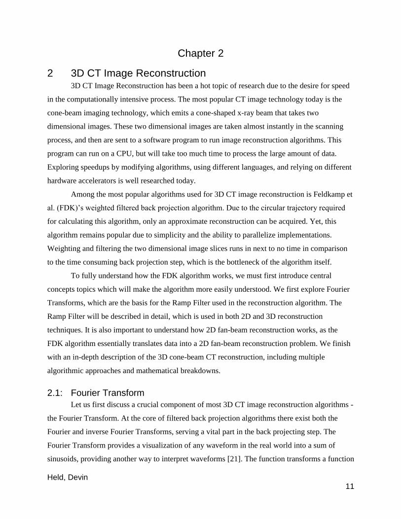
In this paper, the discrete Fourier Transform will be used and the transform of function

f(x) is denoted by F(x). The Fourier Transform will transform functions in the time domain to the

frequency domain for use in back projection and filtering within 3D CT image reconstruction

algorithms. In terms of the sample k in the time domain and N frequencies over the sampling

period, the equations for discrete Fourier Transform and inverse Fourier transform are as

follows:

Figure 5: Fourier Transform Equations (Credit: roymech.co.uk).

The value of N is the sampling period and is the same as the number of pixels in the x-direction

of the image (i.e. 2563 image would have a sampling period of 256). The equation appears

complicated, but in simple English, this equation allows you to find the frequency at F(n)

through spinning (e-i) the sample k around the circle (defined by 2π) and averaging point values

along the path ( ∑ ). The run time complexity of this algorithm is O(nlogn). The Fourier

Transform in back projection algorithms for both two and three dimensional transforms will take

on a different form but the logic will remain the same. Image filtering is applied to the frequency

domain, which is why the Fourier Transform is a vital part of the algorithm.

2.2: Ramp Filtering

Another vital concept to understand prior to discussing reconstruction algorithms is the

Ramp Filter. The Ramp Filter is a high-pass filter, increasing frequencies above the cut off and

decreasing low frequencies. It is used to create a clearer image without changing projection data

before the back projection step. This filter assists in reducing blur and other visual artifacts

found in the projection images. The Ramp Filter, defined by the inverse Fourier Transform,

http://roymech.co.uk/

Held, Devin 13

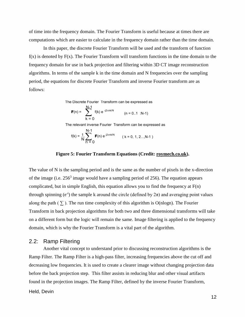
targets image noise and imperfections and smooths them out through filtering techniques. The

Ramp Filter calculates the absolute value of the frequencies and rolls off at a certain point. It is

demonstrated in the following diagram:

[31]

First, the Fourier Transform is calculated, then the Ramp Filter is evaluated, and then the inverse

Fourier Transform is calculated. The core of the Ramp Filter equation is written as follows:

[31]

As this equation is applied to the frequency domain (after application of the Fourier Transform)

kx and ky represent the frequencies at a certain point. The Ramp Filter effectively attenuates

frequencies below a cut off factor, however, it can leave the image considerably grainy. Because

of this, the Ramp Filter must be combined with a Cosine Function to deemphasize noise. The

Cosine Function is defined as follows:

C(k) = ½ * (1 – cos((2 * π * k) / (k – 1)))

[31]

where k is the Ramp Filter frequency.

Held, Devin 14

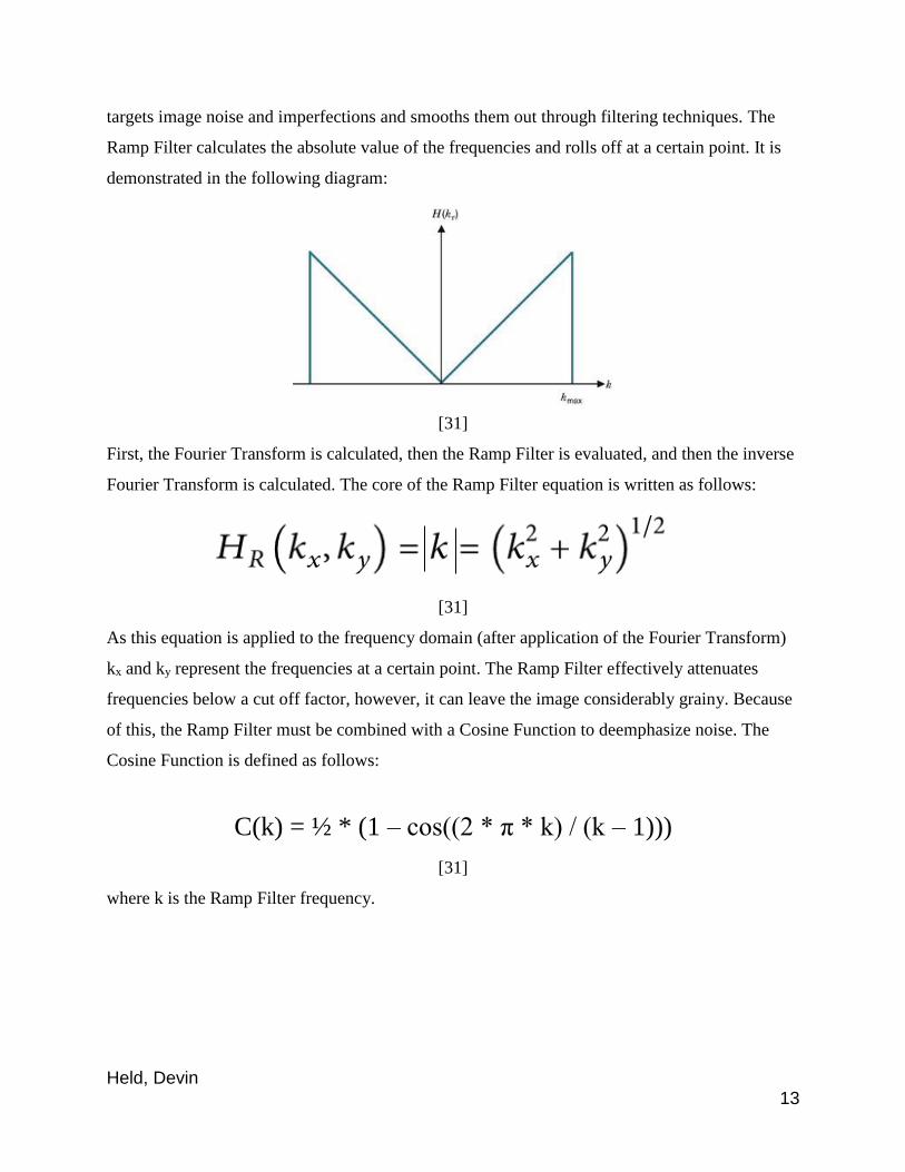
To understand why the Ramp Filter is necessary in back projection algorithms, let us

analyze the following images:

(a) (b)

(c)

Figure 6: (a) Original image, (b) unfiltered back projected image, and (c) ramp filtered

image. (Credit: www.clear.rice.edu).

Image (a) represents the original phantom image prior to unfiltered back projection

reconstruction in the image (b). Due to the overlapping of image slices that have undergone the

Fourier Transform, the resulting image is very unclear [22]. Because of this, a high-pass filter,

such as the Ramp Filter, must be applied to attenuate the lower frequencies and keep the higher

frequencies in the image. The lower frequencies cause blur, and therefore data must be passed

through a high-pass filter to reduce the blurring. Image (c) is the result of applying the Ramp

Filter to the back projected image. Note that the resulting image in (c) is considerably grainy -

this is smoothed out by multiplying the filter by the Cosine Function (defined above) to

deemphasize noise.

http://www.clear.rice.edu/

Held, Devin 15

2.3: Fan Beam CT Image Reconstruction

A common geometry for x-ray CT is fan-beam imaging technology. As described in

section 1.2.2, fan-beam x-ray CT scans involve collecting data through a x-ray fan projection of

a particular object where the main focal point is the source of the x-ray. Through a mathematical

image reconstruction process, the data is translated into a two dimensional image for the

radiologist to analyze. The underlying logic for fan-beam reconstruction is the basis for cone-

beam image reconstruction, which will be described in section 3.5. Fan-beam CT is preferred

due to the ability to capture greater definition of soft tissue and bones.

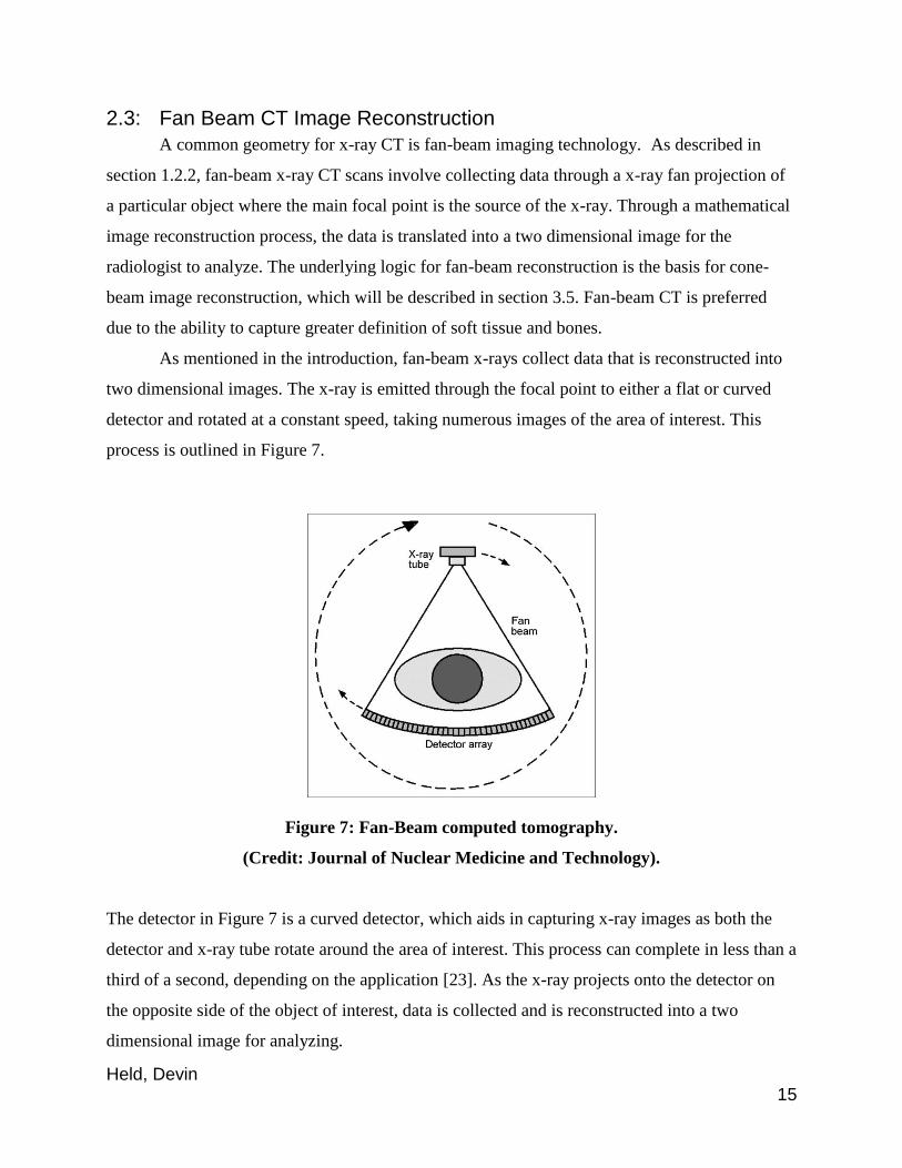
As mentioned in the introduction, fan-beam x-rays collect data that is reconstructed into

two dimensional images. The x-ray is emitted through the focal point to either a flat or curved

detector and rotated at a constant speed, taking numerous images of the area of interest. This

process is outlined in Figure 7.

Figure 7: Fan-Beam computed tomography.

(Credit: Journal of Nuclear Medicine and Technology).

The detector in Figure 7 is a curved detector, which aids in capturing x-ray images as both the

detector and x-ray tube rotate around the area of interest. This process can complete in less than a

third of a second, depending on the application [23]. As the x-ray projects onto the detector on

the opposite side of the object of interest, data is collected and is reconstructed into a two

dimensional image for analyzing.

Held, Devin 16

2.3.1: Algorithm and Mathematical Analysis

Typical fan-beam reconstruction algorithms use the Fourier Transform and Ramp

Filtering to effectively attenuate lower frequencies, which enhances image sharpness (as

demonstrated in Figure 9). The algorithm itself is important to understand because it is the basis

for the Feldkamp et al. 3D CT image reconstruction algorithm, which is the focus of this thesis.

Each image slice taken by the x-ray projection must be filtered, weighted, and back projected in

order to compile the two dimensional object of interest.

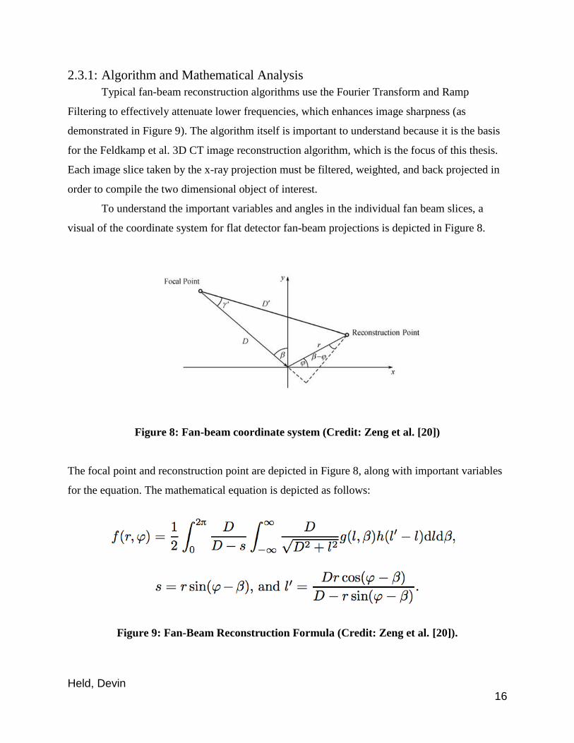
To understand the important variables and angles in the individual fan beam slices, a

visual of the coordinate system for flat detector fan-beam projections is depicted in Figure 8.

Figure 8: Fan-beam coordinate system (Credit: Zeng et al. [20])

The focal point and reconstruction point are depicted in Figure 8, along with important variables

for the equation. The mathematical equation is depicted as follows:

Figure 9: Fan-Beam Reconstruction Formula (Credit: Zeng et al. [20]).

Held, Devin 17

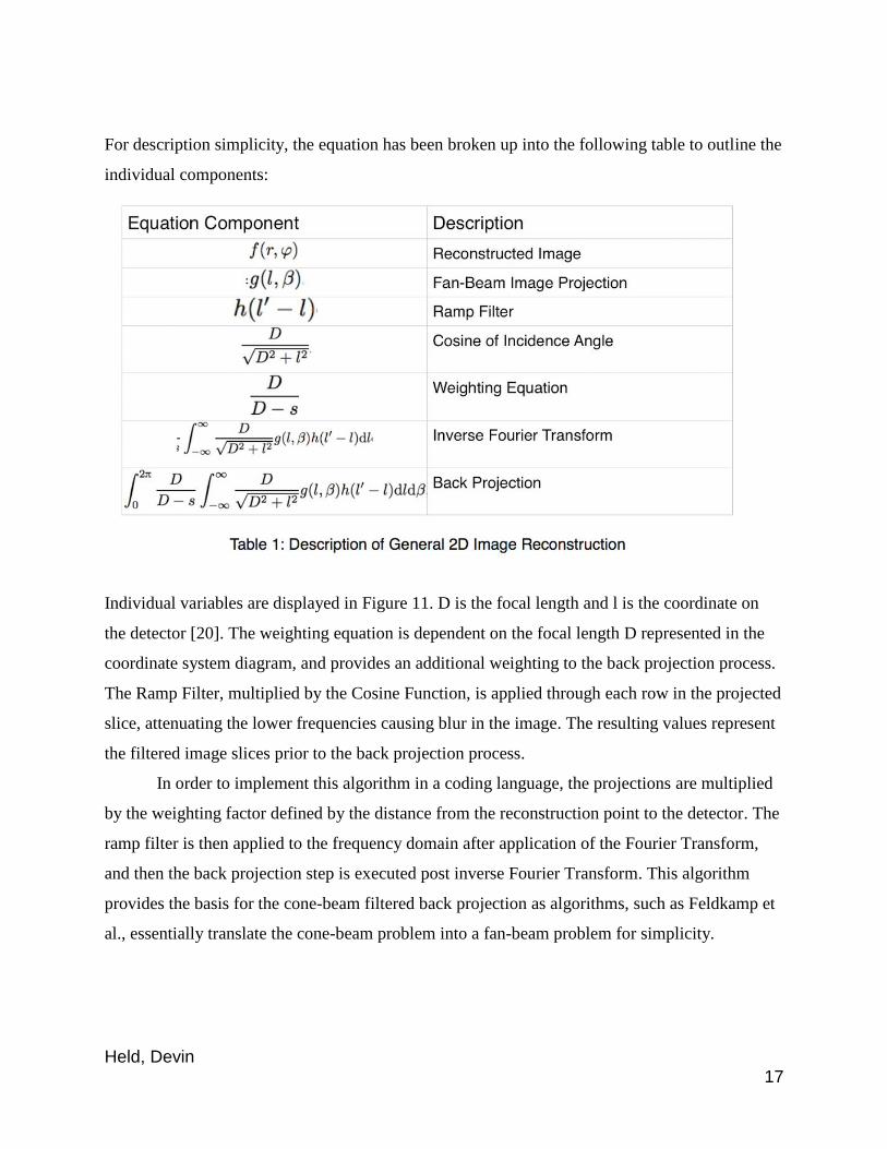
For description simplicity, the equation has been broken up into the following table to outline the

individual components:

Individual variables are displayed in Figure 11. D is the focal length and l is the coordinate on

the detector [20]. The weighting equation is dependent on the focal length D represented in the

coordinate system diagram, and provides an additional weighting to the back projection process.

The Ramp Filter, multiplied by the Cosine Function, is applied through each row in the projected

slice, attenuating the lower frequencies causing blur in the image. The resulting values represent

the filtered image slices prior to the back projection process.

In order to implement this algorithm in a coding language, the projections are multiplied

by the weighting factor defined by the distance from the reconstruction point to the detector. The

ramp filter is then applied to the frequency domain after application of the Fourier Transform,

and then the back projection step is executed post inverse Fourier Transform. This algorithm

provides the basis for the cone-beam filtered back projection as algorithms, such as Feldkamp et

al., essentially translate the cone-beam problem into a fan-beam problem for simplicity.

Held, Devin 18

2.4: Cone Beam CT Image Reconstruction

Cone-Beam CT is a newer technology compared to Fan-Beam CT and implements an

advanced approach to CT scan data collection and reconstruction [13]. Although Cone-Beam

CT (CBCT) reconstructs three dimensional images rather than two dimensional images in Fan-

Beam CT, much of the underlying logic is similar, and therefore can be seen as an advancement

to the Fan-Beam process. Actually, the algorithm translates the 3D cone-beam problem into a

fan-beam problem to evaluate. CBCT was developed to provide more informative and rapid

acquisition of data as compared to Fan-Beam CT, as it results in a three dimensional image

covering the entire field of view [13].

Since CBCT captures two dimensional images rather than data to be reconstructed, it is

prone to many more artifacts than traditional Fan-Beam CT technology. Because of this, a more

intensive mathematical filtering process is applied to each CBCT projection to effectively reduce

appearance of artifacts in the images. The main troublesome artifacts, noise and contrast

imperfections, are more apparent in CBCT projections due to the higher amount of radiation

present [13]. These artifacts must be smoothed through image processing applications or image

clarity will be impaired.

2.4.1: Reconstruction Process

The process of CT image reconstruction begins with acquiring the data from the Cone-

Beam CT (CBCT) scanner, and then reconstructing the two dimensional images. This process

not only creates the three dimensional representation of an object, but also essentially reduces the

artifacts in the images. To simplify the overall process, Figure 10 outlines the dual stage process,

describing the steps involved in each stage.

Held, Devin 19

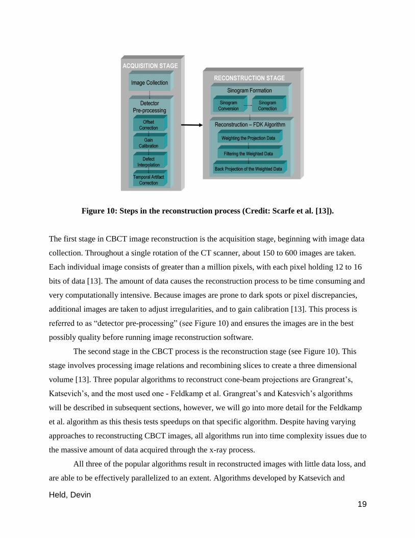
Figure 10: Steps in the reconstruction process (Credit: Scarfe et al. [13]).

The first stage in CBCT image reconstruction is the acquisition stage, beginning with image data

collection. Throughout a single rotation of the CT scanner, about 150 to 600 images are taken.

Each individual image consists of greater than a million pixels, with each pixel holding 12 to 16

bits of data [13]. The amount of data causes the reconstruction process to be time consuming and

very computationally intensive. Because images are prone to dark spots or pixel discrepancies,

additional images are taken to adjust irregularities, and to gain calibration [13]. This process is

referred to as “detector pre-processing” (see Figure 10) and ensures the images are in the best

possibly quality before running image reconstruction software.

The second stage in the CBCT process is the reconstruction stage (see Figure 10). This

stage involves processing image relations and recombining slices to create a three dimensional

volume [13]. Three popular algorithms to reconstruct cone-beam projections are Grangreat’s,

Katsevich’s, and the most used one - Feldkamp et al. Grangreat’s and Katesvich’s algorithms

will be described in subsequent sections, however, we will go into more detail for the Feldkamp

et al. algorithm as this thesis tests speedups on that specific algorithm. Despite having varying

approaches to reconstructing CBCT images, all algorithms run into time complexity issues due to

the massive amount of data acquired through the x-ray process.

All three of the popular algorithms result in reconstructed images with little data loss, and

are able to be effectively parallelized to an extent. Algorithms developed by Katsevich and

Held, Devin 20

Greangreat provide exact image reconstructions, but Feldkamp et al. provide approximate image

reconstructions. To understand the idea of approximate and exact reconstructions, it is important

to understand Tuy’s condition, described in the next section.

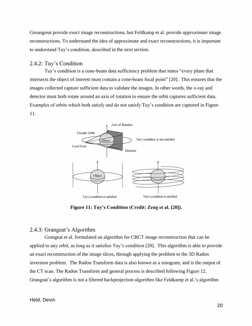
2.4.2: Tuy’s Condition

Tuy’s condition is a cone-beam data sufficiency problem that states “every plane that

intersects the object of interest must contain a cone-beam focal point” [20]. This ensures that the

images collected capture sufficient data to validate the images. In other words, the x-ray and

detector must both rotate around an axis of rotation to ensure the orbit captures sufficient data.

Examples of orbits which both satisfy and do not satisfy Tuy’s condition are captured in Figure

11.

Figure 11: Tuy’s Condition (Credit: Zeng et al. [20]).

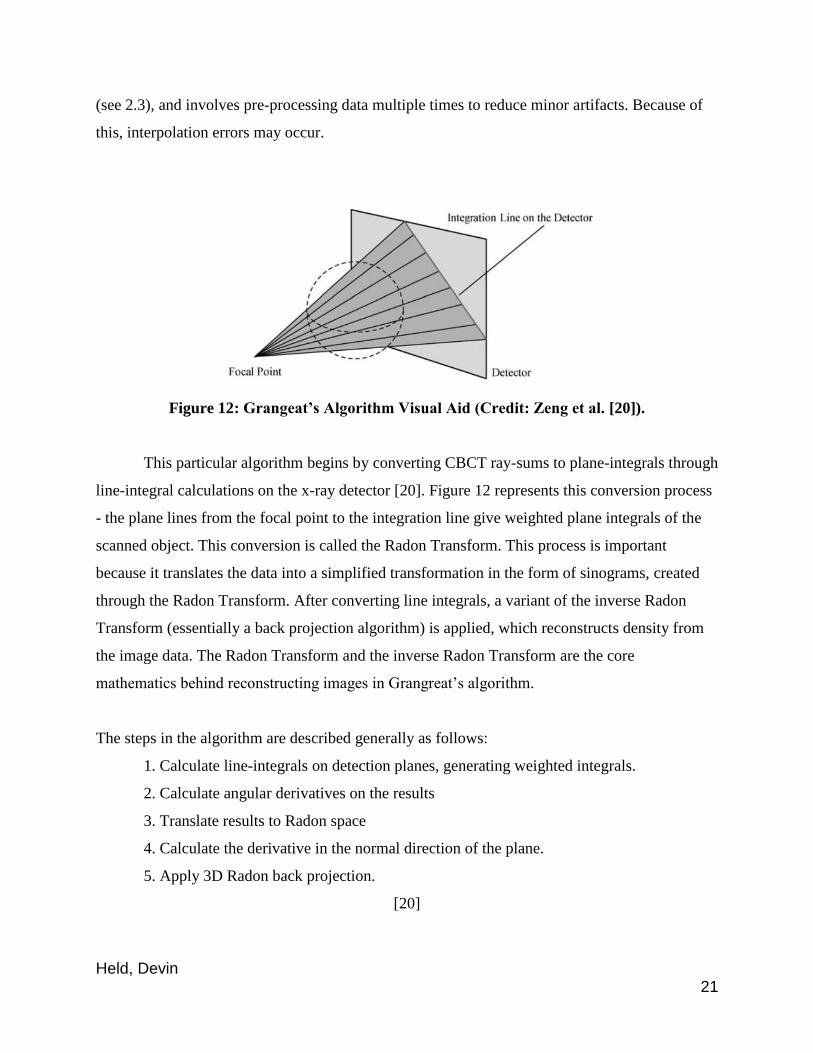
2.4.3: Grangeat’s Algorithm

Grangeat et al. formulated an algorithm for CBCT image reconstruction that can be

applied to any orbit, as long as it satisfies Tuy’s condition [20]. This algorithm is able to provide

an exact reconstruction of the image slices, through applying the problem to the 3D Radon

inversion problem. The Radon Transform data is also known as a sinogram, and is the output of

the CT scan. The Radon Transform and general process is described following Figure 12.

Grangeat’s algorithm is not a filtered backprojection algorithm like Feldkamp et al.’s algorithm

Held, Devin 21

(see 2.3), and involves pre-processing data multiple times to reduce minor artifacts. Because of

this, interpolation errors may occur.

Figure 12: Grangeat’s Algorithm Visual Aid (Credit: Zeng et al. [20]).

This particular algorithm begins by converting CBCT ray-sums to plane-integrals through

line-integral calculations on the x-ray detector [20]. Figure 12 represents this conversion process

- the plane lines from the focal point to the integration line give weighted plane integrals of the

scanned object. This conversion is called the Radon Transform. This process is important

because it translates the data into a simplified transformation in the form of sinograms, created

through the Radon Transform. After converting line integrals, a variant of the inverse Radon

Transform (essentially a back projection algorithm) is applied, which reconstructs density from

the image data. The Radon Transform and the inverse Radon Transform are the core

mathematics behind reconstructing images in Grangreat’s algorithm.

The steps in the algorithm are described generally as follows:

1. Calculate line-integrals on detection planes, generating weighted integrals.

2. Calculate angular derivatives on the results

3. Translate results to Radon space

4. Calculate the derivative in the normal direction of the plane.

5. Apply 3D Radon back projection.

[20]

Held, Devin 22

Mathematical details will not be expressed in this paper, as the purpose of summarizing

this algorithm is to outline the differences between it and the popular CBCT reconstruction

algorithms.

2.4.4: Katsevich’s Algorithm

Katsevich’s algorithm follows the filtered back projection pattern, but can be altered to

remove the dependence of the filter on the reconstruction location [20]. In general, it involves

calculating important values based on the location of the object and the orbit, then introducing

the Hilbert Transform and additional weighting to reduce visual artifacts. The transform runs in

O(n2) time in comparison to the Fourier Transform time which runs in O(nlogn) time. The

Hilbert Transform provides an analytic representation of a specified signal, defined for functions

on a circle, as we see here with the helical orbit used by this algorithm. Mathematical details will

not be discussed as the purpose of outlining this algorithm is to compare the process with

Feldkamp et al’s.

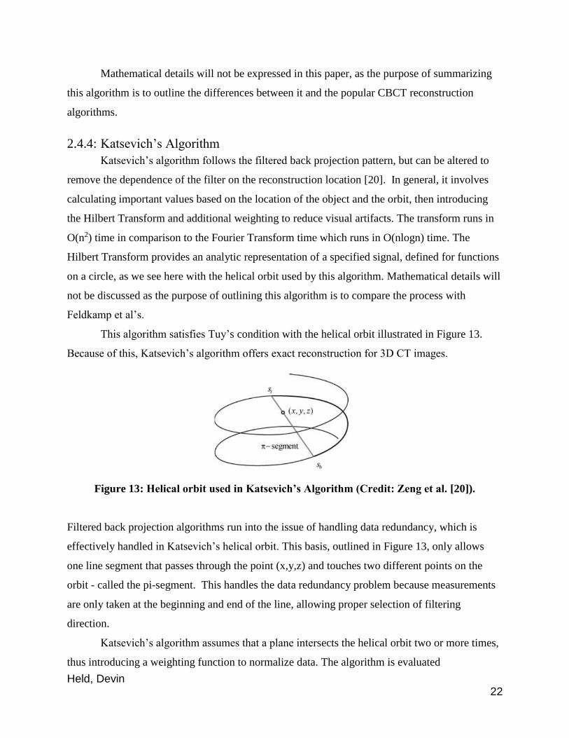
This algorithm satisfies Tuy’s condition with the helical orbit illustrated in Figure 13.

Because of this, Katsevich’s algorithm offers exact reconstruction for 3D CT images.

Figure 13: Helical orbit used in Katsevich’s Algorithm (Credit: Zeng et al. [20]).

Filtered back projection algorithms run into the issue of handling data redundancy, which is

effectively handled in Katsevich’s helical orbit. This basis, outlined in Figure 13, only allows

one line segment that passes through the point (x,y,z) and touches two different points on the

orbit - called the pi-segment. This handles the data redundancy problem because measurements

are only taken at the beginning and end of the line, allowing proper selection of filtering

direction.

Katsevich’s algorithm assumes that a plane intersects the helical orbit two or more times,

thus introducing a weighting function to normalize data. The algorithm is evaluated

Held, Devin 23

independently on each projection slice, which amounts to calculating results on each 2D image

by the intersecting plane. Katsevich’s algorithm [20] is described as follows:

1. Find derivative of data with respect to orbit parameter.

2. Calculate the Hilbert transform.

3. Perform weighted back projection.

Mathematical details of this algorithm are not presented here, as this thesis is working

with the Feldkamp et al. algorithm described in section 2.3.

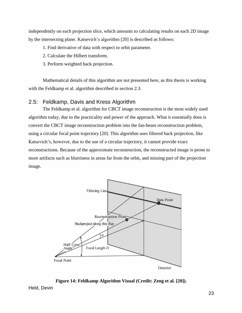
2.5: Feldkamp, Davis and Kress Algorithm

The Feldkamp et al. algorithm for CBCT image reconstruction is the most widely used

algorithm today, due to the practicality and power of the approach. What it essentially does is

convert the CBCT image reconstruction problem into the fan-beam reconstruction problem,

using a circular focal point trajectory [20]. This algorithm uses filtered back projection, like

Katsevich’s, however, due to the use of a circular trajectory, it cannot provide exact

reconstructions. Because of the approximate reconstruction, the reconstructed image is prone to

more artifacts such as blurriness in areas far from the orbit, and missing part of the projection

image.

Figure 14: Feldkamp Algorithm Visual (Credit: Zeng et al. [20]).

Held, Devin 24

Figure 14 provides a visualization of the Feldkamp algorithm, outlining the cone-beam

projections and where the filter and back projections are applied. Feldkamp et. al (FDK) utilizes

the cone angle outlined in Figure 16 and gives exact reconstruction if the angle is less than ten

degrees or if the scanned object has constant dimensions in one direction [20].

2.5.1: Algorithm and Mathematical Analysis

As mentioned before, the FDK algorithm implements filtered back projection, heavily

relying on the conversion from a cone-beam reconstruction problem to a modified fan-beam

reconstruction problem. Steps described in the FDK cone-beam algorithm may sound similar to

that in fan-beam reconstruction techniques. The general algorithm [20] is described as follows:

1. Scale projections by cosine of the cone angle.

2. Apply ramp filtering to the data.

3. Apply weighted-filtered back projection.

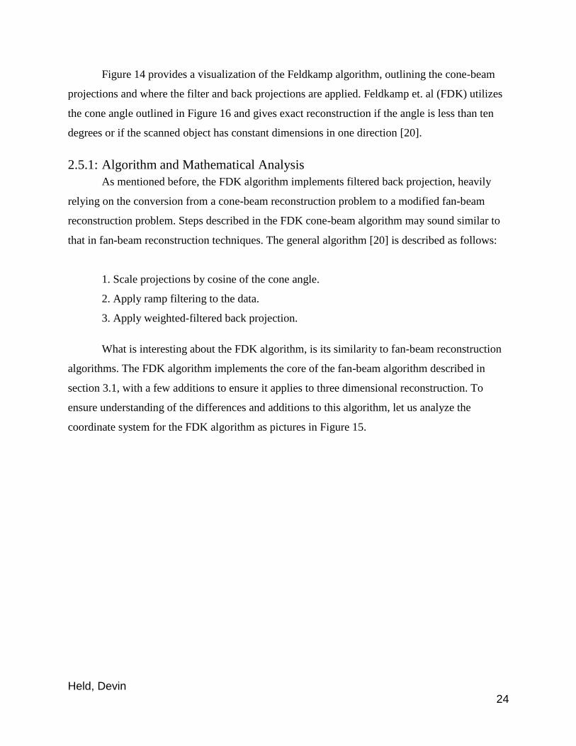
What is interesting about the FDK algorithm, is its similarity to fan-beam reconstruction

algorithms. The FDK algorithm implements the core of the fan-beam algorithm described in

section 3.1, with a few additions to ensure it applies to three dimensional reconstruction. To

ensure understanding of the differences and additions to this algorithm, let us analyze the

coordinate system for the FDK algorithm as pictures in Figure 15.

Held, Devin 25

Figure 15: Cone-Beam Coordinate System (Credit: Zeng et al. [20]).

The difference between the cone-beam coordinate system and the fan-beam coordinate system

(see Figure 8) is the addition of a dimension in the z direction and abstraction of the

reconstruction point to fit the three dimensions. The cone-beam coordinate system is similar to

the fan-beam coordinate system. However, an additional dimension - z - is added to the diagram

to represent the third dimension of the cone-beam projection. An important variable to note is

the length from the detector to the focal point, D, which is the main determination of a weighting

function for this algorithm.

In terms of the algorithms, the only difference is that the back projection is a cone-beam

back projection. CBCT also uses the Fourier transform and ramp filtering to reconstruct the CT

images. Ramp-filtering is applied to the images row-by-row and then back projection is

calculated on the resulting data. Zeng et al. [20] provide an exceptional straightforward diagram

of the cone-beam coordinate systems and a clear mathematical equation to assist in

understanding and expressing important aspects.

Held, Devin 26

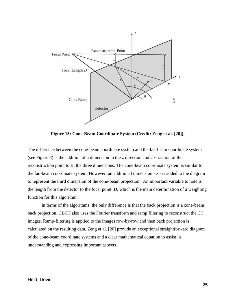
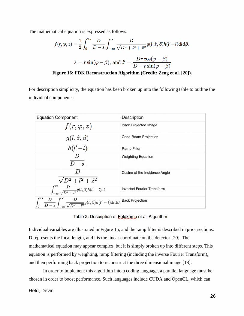
The mathematical equation is expressed as follows:

Figure 16: FDK Reconstruction Algorithm (Credit: Zeng et al. [20]).

For description simplicity, the equation has been broken up into the following table to outline the

individual components:

Individual variables are illustrated in Figure 15, and the ramp filter is described in prior sections.

D represents the focal length, and l is the linear coordinate on the detector [20]. The

mathematical equation may appear complex, but it is simply broken up into different steps. This

equation is performed by weighting, ramp filtering (including the inverse Fourier Transform),

and then performing back projection to reconstruct the three dimensional image [18].

In order to implement this algorithm into a coding language, a parallel language must be

chosen in order to boost performance. Such languages include CUDA and OpenCL, which can

Held, Devin 27

conveniently run on a graphics processing unit (GPU) to increase performance. Since, this

algorithm has potential to be highly parallelized due to data independence, running such an

algorithm on an accelerator is promising [18]. Design wise, the projections are first multiplied

with the weighting function. The ramp filter is then applied to the data and finally back

projection is performed. Both the run times of weighting and ramp filtering run in O(N2) while

the computationally intensive back projection step that runs in O(N4) time [15]. This run time is

a result of traversing through each projection in the image, through each individual pixel in the

projection, and then through each angle taken during data collection. Implementation pseudo

code will be described in Chapter 5 along with benchmarking the run times.

2.6: Performance Bottlenecks

The process of 3D CT image reconstruction is a computationally expensive process and

so there exists multiple bottlenecks preventing desirable performance. The main motivation for

implementing algorithms, such as FDK back projection on accelerators, is to dramatically

improve run-time of the intensive back projection step. The back projection step is the most

difficult to make computationally efficient, as the number of computations required to compute

this step is rather large. As the size of the data set grows, and it is very large with full CT scans,

the O(n4) complexity of this step takes quite a while to compute.

With the move to GPUs, the back projection step has conclusively sped up the overall run

time. Yet, in using an accelerator, such as the GPU, a new bottleneck surfaces. Projection data

must be loaded onto the accelerator in order to run computations on the device, thus creating the

memory transfer bottleneck. The question then becomes - how do we implement efficient

memory transfer? This bottleneck can be reduced through transferring data all at once and doing

as many computations as possible on the GPU before inducing another single transfer back to the

CPU. But, with the exceptionally large size of the CT scan data files, this still results in

considerable overhead.

What is interesting to further explore is if the field programmable gate array (FPGA) is

able to further reduce run time of this algorithm and overcome the runtime bottleneck. It is also

interesting to explore whether the use of a Power8 along with the FPGA is able to improve the

bottleneck of memory transfer through providing a more fluid memory transfer process. These

bottlenecks, while not as apparent in GPU implementations compared to pure CPU

Held, Devin 28

implementations, are a means to further investigate this popular FDK reconstruction algorithm

and discern whether further speed ups are feasible.

Held, Devin 29

Chapter 3

3 Related Work As mentioned in the previous chapter, 3D CT scan image reconstruction has been a

largely researched topic due to the desire for efficiency in the implementations. Feldkamp’s

algorithm for back projection in image reconstruction [3] has been the core for the majority of

research studies due to its efficiency and its suitability to parallel processing, thus harnessing the

power of accelerators such as the GPU and FPGA [14]. The bottleneck of this algorithm, the

back projection step, has a runtime complexity of O(N4) and has been the focus of many research

studies [15]. Along with this algorithmic complexity, there exists another more pragmatic

bottleneck - memory transfer between accelerators and the central processing unit (CPU).

The following survey of related research studies are all focused on the Feldkamp et al.

back projection algorithm for image reconstruction [3]. This is the most commonly used

algorithm today due to the practicality and power of approach. The algorithm itself is described

in Chapter 2. The majority of studies on this problem are implemented on the GPU in either

CUDA or OpenCL. The first three research studies outline GPU implementations. The use of the

FPGA for this particular algorithm is minimal, and the use of the Power8 is nonexistent. The

fourth and final research study surveyed outlines an implementation on the FPGA. However, it

uses a simulated memory bus and does not utilize OpenCL nor Power8 processing technology.

3.1: Related Work 1 - “Accelerated cone-beam CT reconstruction based on OpenCL” by Wang et al. [18]

As mentioned in the prior section, exploring cone-beam CT reconstruction algorithms on

the graphics processing unit (GPU) is a well-researched topic as the GPU has capabilities to

speed up reconstruction algorithms considerably. Wang et al. [18] benchmark the Feldkamp et al.

algorithm through a parallel implementation for the GPU. Unlike many implementations of this

algorithm, they decided to use OpenCL to write the device code for the GPU. The relatively new

OpenCL language has not been thoroughly researched for applications such as for the FDK

algorithm performance speedups. The parallel capabilities of the OpenCL language make it a

valuable choice for optimizing implementations for accelerator hardware.

Held, Devin 30

3.1.1: Implementation

The implementation was designed to be parallel to work with the OpenCL model.

OpenCL was the implementation language of choice because it can work across many different

GPUs, while implementations in compute unified device architecture (CUDA) are typically

restricted for use on NVIDIA or AMD GPUs [18]. With OpenCL, the ability to develop generic

algorithms to work cross platforms is more plausible, and such code can also be run on multiple

hardware devices such as the CPU, GPU, and FPGA. The ability to abstract sections of the

algorithm into device code contained in kernels ensures that the developer has a clear sense of

what is running where and how to write code to run on both the CPU and GPU at the same time.

To minimize data transfer between the CPU and GPU, which is inevitable due to the

storage capacity on the GPU, Wang et al. introduced pinned (also called page-locked) memory to

store the image slices rather than non-pinned memory [18]. Both pinned and non-pinned memory

are ways the GPU accesses memory from the host device. Pinned memory is quicker due to the

ability to execute writes and application instructions concurrently, and large sequential reading

[32]. Non-pinned memory invokes multiple levels of caching, involving full loads of data [32].

Non-pinned memory seems less useful in this case due to the change of data throughout the

reconstruction process. Kernels were designed to run each of the steps in the FDK algorithm, as

described in Chapter 3. Image-by-image, data is loaded onto the GPU, with kernels executing

pre-weighting, filtering, reconstruction, and weighting before transferring the data back to the

GPU. Running all GPU computations at the same time reduces the need to transfer data multiple

times which would inhibit performance.

3.1.2: Conclusions

Based on benchmarking the OpenCL implementation of the FDK algorithm on the CPU

compared to the GPU, Wang et al. produced an overall speedup of over 57 times. To test, they

used a generated head phantom with 1283 voxels. As the volume of the data increased, the

speedup numbers also increased. With a head phantom of 2563 voxels, the GPU implementation

performed 250 times better than the CPU implementation for the weighting step! With these

tests, it is clear that implementing the FDK algorithm in OpenCL for the GPU provides dramatic

improvements in performance. Although OpenCL is a relatively new language to use for GPU

programming, it has potential to allow creation of complex algorithms run more fluidly through

efficient parallelization [18].

Held, Devin 31

3.2: Related Work 2 - “GPU-based cone beam computer tomography” by Noel et al. [17]

Though the time it takes to scan images for 3D cone-beam CT procedures is merely 60

seconds, the images must run through timely reconstruction software, which can take upwards of

25 minutes on a typical workstation desktop [17]. Noel et al. approached the computationally

intense 3D cone-beam reconstruction by implementing the Feldkamp et al. (FDK) algorithm on

the graphics processing unit (GPU). The Compute Unified Device Architecture (CUDA) is used

to parallelize both the filtering step and the intensive back projection step on the GPU. The core

of the paper evaluates the run time of the CUDA implementation on the CPU vs. the GPU with a

straight forward algorithmic approach. Multiple volume sizes are tested on both the CPU and

GPU to compare speedup numbers.


The weight-filtered-FDK algorithm, described as a “simple implementation”, was

implemented in CUDA for a CUDA-capable GPU. Specific tests were run on a cheap GPU - the

NVIDIA GeForce GTX 280, making the results relevant to real world applications due to the

low-cost of the device. The approach consists of harnessing all shared memory, loading all of the

image data in the memory on the GPU device, and parallelizing computations on individual

voxels.

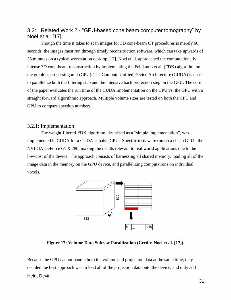
Figure 17: Volume Data Subrow Parallization (Credit: Noel et al. [17]).

Because the GPU cannot handle both the volume and projection data at the same time, they

decided the best approach was to load all of the projection data onto the device, and only add

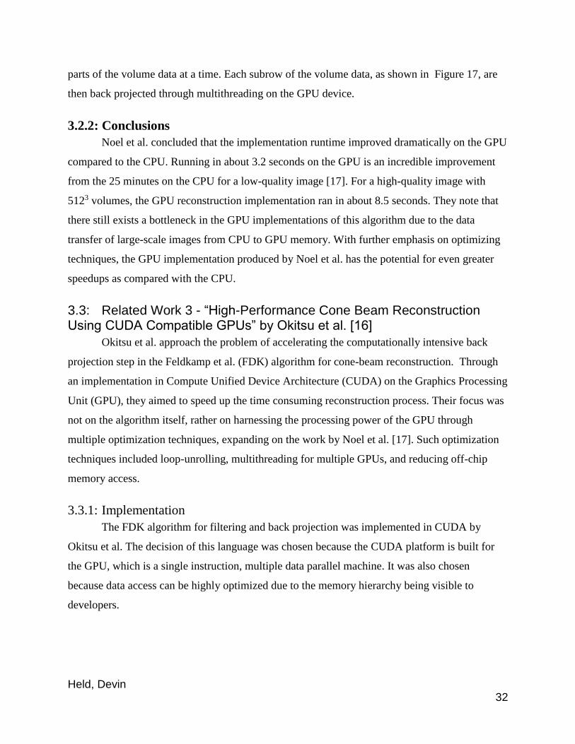
Held, Devin 32

parts of the volume data at a time. Each subrow of the volume data, as shown in Figure 17, are

then back projected through multithreading on the GPU device.

3.2.2: Conclusions

Noel et al. concluded that the implementation runtime improved dramatically on the GPU

compared to the CPU. Running in about 3.2 seconds on the GPU is an incredible improvement

from the 25 minutes on the CPU for a low-quality image [17]. For a high-quality image with

5123 volumes, the GPU reconstruction implementation ran in about 8.5 seconds. They note that

there still exists a bottleneck in the GPU implementations of this algorithm due to the data

transfer of large-scale images from CPU to GPU memory. With further emphasis on optimizing

techniques, the GPU implementation produced by Noel et al. has the potential for even greater

speedups as compared with the CPU.

3.3: Related Work 3 - “High-Performance Cone Beam Reconstruction Using CUDA Compatible GPUs” by Okitsu et al. [16]

Okitsu et al. approach the problem of accelerating the computationally intensive back

projection step in the Feldkamp et al. (FDK) algorithm for cone-beam reconstruction. Through

an implementation in Compute Unified Device Architecture (CUDA) on the Graphics Processing

Unit (GPU), they aimed to speed up the time consuming reconstruction process. Their focus was

not on the algorithm itself, rather on harnessing the processing power of the GPU through

multiple optimization techniques, expanding on the work by Noel et al. [17]. Such optimization

techniques included loop-unrolling, multithreading for multiple GPUs, and reducing off-chip

memory access.


The FDK algorithm for filtering and back projection was implemented in CUDA by

Okitsu et al. The decision of this language was chosen because the CUDA platform is built for

the GPU, which is a single instruction, multiple data parallel machine. It was also chosen

because data access can be highly optimized due to the memory hierarchy being visible to

developers.

Held, Devin 33

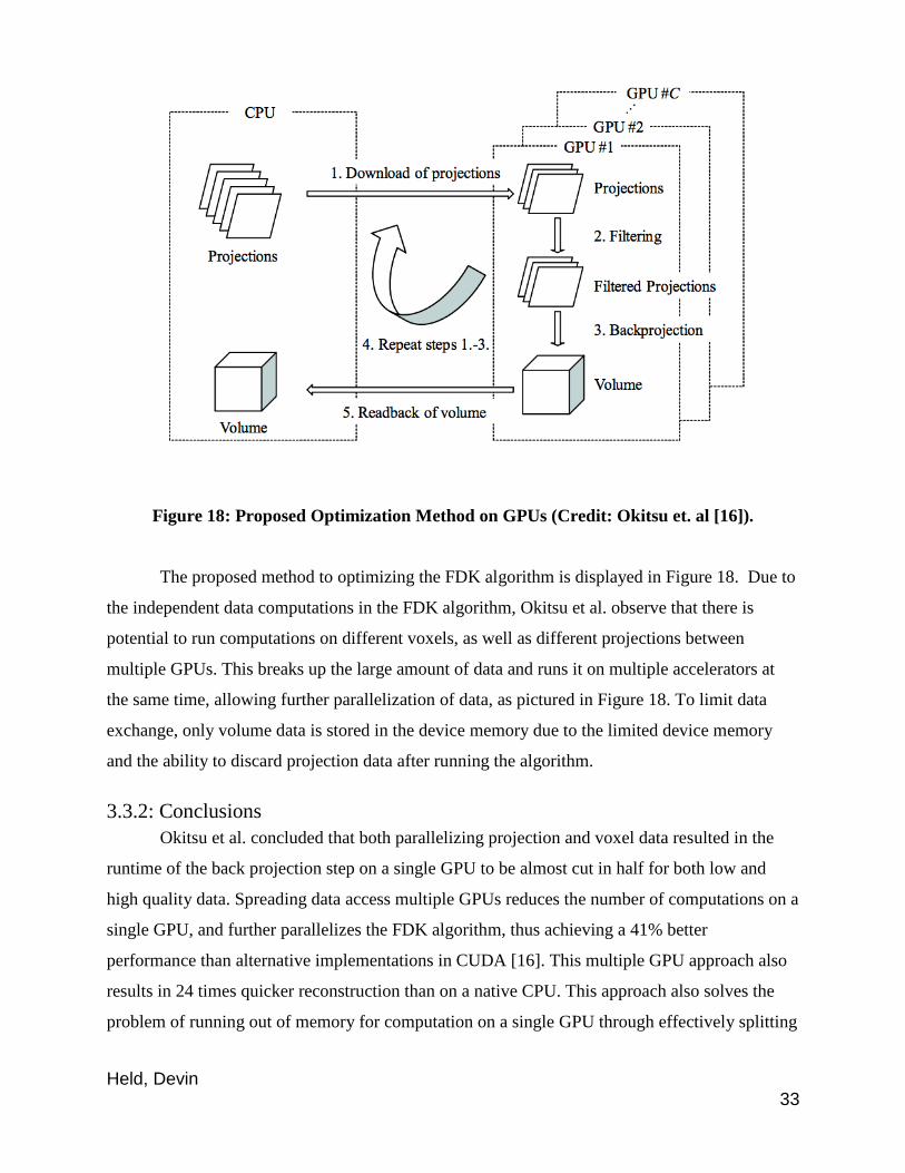
Figure 18: Proposed Optimization Method on GPUs (Credit: Okitsu et. al [16]).

The proposed method to optimizing the FDK algorithm is displayed in Figure 18. Due to

the independent data computations in the FDK algorithm, Okitsu et al. observe that there is

potential to run computations on different voxels, as well as different projections between

multiple GPUs. This breaks up the large amount of data and runs it on multiple accelerators at

the same time, allowing further parallelization of data, as pictured in Figure 18. To limit data

exchange, only volume data is stored in the device memory due to the limited device memory

and the ability to discard projection data after running the algorithm.

3.3.2: Conclusions

Okitsu et al. concluded that both parallelizing projection and voxel data resulted in the

runtime of the back projection step on a single GPU to be almost cut in half for both low and

high quality data. Spreading data access multiple GPUs reduces the number of computations on a

single GPU, and further parallelizes the FDK algorithm, thus achieving a 41% better

performance than alternative implementations in CUDA [16]. This multiple GPU approach also

results in 24 times quicker reconstruction than on a native CPU. This approach also solves the

problem of running out of memory for computation on a single GPU through effectively splitting

Held, Devin 34

up the data, as large-scale datasets can easily diminish resources in a single GPU device

memory.

3.4: Related Work 4 - “High speed 3D tomography on CPU, GPU, and FPGA” by Gac et al. [19]

Gac et al. experiment with implementations of similar 3D CT and 3D PET image

reconstruction algorithms on the CPU, GPU, and FPGA hardware environments. The back

projection of both types of image reconstruction is costly, and this paper explores optimization

techniques for the implementing on the FPGA hardware. They approach the memory access

bottleneck, designing a pipeline that improves efficiency. This is among a few studies done with

the 3D image reconstruction problem on the FPGA, comparing speedups in comparison with

both the CPU and GPU.


Three versions of the back projection software program were implemented on the CPU -

two optimized, and one not. The optimized versions used multiple techniques, including better

utilization of cache memory, and reduction of arithmetic operations. With the implementation

making better utilization of cache memory, they induced a speedup of 3-fold; a speedup of 7-fold

was achieved through the addition of arithmetic operation reduction [19].

“Standard C with a few extensions” was used to program the GPU code, which could be

either OpenCL or CUDA. Their implementation involved assigning a single thread to each voxel,

or tomographic image, and performing reconstruction in blocks. Two implementations of the

parallel code were written, with simple loop manipulation the difference between the two. The

simple loop manipulation reduced the number of computations between image coordinates, thus

induced a speedup of 2 times the original GPU implementation.

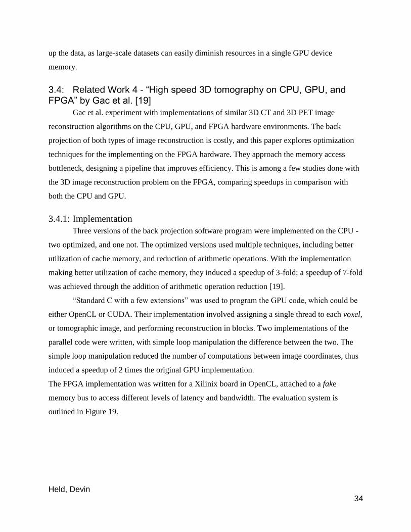
The FPGA implementation was written for a Xilinix board in OpenCL, attached to a fake

memory bus to access different levels of latency and bandwidth. The evaluation system is

outlined in Figure 19.

Held, Devin 35

Figure 19: FPGA Evaluation System (Credit: Gac et al. [19]).

As illustrated in Figure 19, the FPGA (Virtex II pro) is attached to an evaluation board

containing multiple memory chips. This allows Gac et al. to effectively control the memory bus

connecting the FPGA board and the host PC. This system can induce an image update in simply

1 clock cycle, allowing the cache to “take advantage of the high spatial and temporal locality” of

the 3D back projection algorithm [19]. They found that the reconstruction ran more slowly when

more threads were running back projection concurrently, as the memory bus was overloaded

with information. The implementation ran most efficient with 8 bytes/cycle memory latency,

with running 1 operation of back projection per processing unit [19].

3.4.2: Conclusions

Gac et al. find that the GPU implementation of the 3D image reconstruction algorithms

runs the quickest at 10 times quicker than the FPGA implementation. However, the FPGA

performed better in computational efficiency with two cycles per instruction [19]. Nonetheless,

the FPGA managed to provide an efficient solution to the bottleneck memory problem and

provide a speedup of approximately 20 times over the general CPU implementations. They

conclude that the few memory resources on the FPGA hardware reduces its ability to handle

such problems in comparison to the GPU, but outperforms the CPU in runtime and efficiency.

Held, Devin 36

They also note that since a GPU is much cheaper than the FPGA, it appears to be a more viable

solution for 3D image reconstruction.

3.5: Summary and Thesis Direction

It appears the most researched ways of speeding up 3D cone-beam image reconstruction

is through implementations in either CUDA or OpenCL for the graphics processing unit (GPU).

All such studies [i.e. 16,17,18,19] resulted in dramatic speedups from running the algorithm on

the GPU in comparison to the CPU. This is due to the parallel nature of the GPU and the ability

to process graphics extremely effectively. Very little work has been done on the field

programmable gate array (FPGA), potentially due to the cost and time consuming development

period.

It is important to note that in the final related work survey, Gac et al. express that the

FPGA performed more poorly than the GPU in 3D image reconstruction due to the memory

resources available and transfer inefficiency. Although they used a simulated memory bus. It is

interesting to explore the outcome of using a Power8 in addition to the FPGA (and a real

memory bus). With Power8 processing technology, better performance could potentially occur

due to the reduction in computing path length to transfer memory from the FPGA to the CPU.

This thesis will explore just that - 3D cone-beam reconstruction implemented on a FPGA

with Power8 processing technology to assist with the memory bottleneck. It is also interesting to

investigate the potential of OpenCL as the implementation language, as previously surveyed

studies all appear to use CUDA and standard C. After describing 3D CT cone-beam

reconstruction algorithms and FPGAs in depth, it will be hopefully be clearer whether there is

the potential for such hardware to speedup the computationally intensive algorithm. However,

the interesting comparison will be between the speedups from a FPGA and a GPU, as both are

able to produce dramatic speedups from the CPU [16,17,18,19].

Held, Devin 37

Chapter 4

4 FPGAs and Power8 With computationally intensive algorithms such as cone-beam CT image reconstruction,

there exists performance limitations with running the algorithm solely on the central processing

unit (CPU). The CPU is able to compute the FDK algorithm, but takes some time to complete

calculations on large data volumes, causing the reconstruction process to prevent the radiologist

from analyzing images immediately. The CPU itself can only handle limited computations

simultaneously, so parallel processing of such algorithms is very limited.

To solve the performance bottleneck of algorithms such as these, the graphics processing

unit (GPU) and recently field programmable gate arrays (FPGAs) have been incorporated to

offload computations off of the CPU. The customizable and parallel nature of such accelerators

allows developers the freedom to write device code that can result in immense performance

speedups when working in unison with the CPU. Both the GPU and FPGA device codes can be

written with little knowledge of low level circuit design by using languages such as CUDA or

OpenCL, which are extensions to the C language. However, FPGA performance is best when

written in a hardware description language such as VHDL, but VHDL has a steep learning curve

because of the need to understand circuit design.

4.1: Field Programmable Gate Arrays (FPGAs)

The field programmable gate array (FPGA) is an integrated circuit customizable by the

developer after the initial manufacturing. FPGAs are used in many varying applications today

such as medical imaging, industrial processing, security, and image processing applications.

Containing a two dimensional array of logic blocks, FPGAs can be programmed to run

combinational functions designed by the developer. The flexible design process appeals to

developers in order to create hardware for specific applications.

The largest FPGA manufacturers are Altera and Xilinx, making up over 90% of total

market share for FPGAs from 2013 and forward [24]. Altera invented the first reconfigurable

hardware device in 1984, a year after they were founded [25], followed by Xilinx releasing the

first commercially available FPGA in 1985 [26]. For many years after, Altera and Xilinx

dominated the FPGA market, and are still the two top manufacturers for the device. An example

of a FPGA board is the Altera Stratix V chip, pictured in Figure 20.

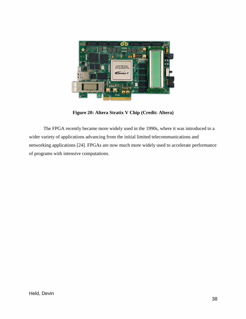
Held, Devin 38

Figure 20: Altera Stratix V Chip (Credit: Altera)

The FPGA recently became more widely used in the 1990s, where it was introduced to a

wider variety of applications advancing from the initial limited telecommunications and

networking applications [24]. FPGAs are now much more widely used to accelerate performance

of programs with intensive computations.

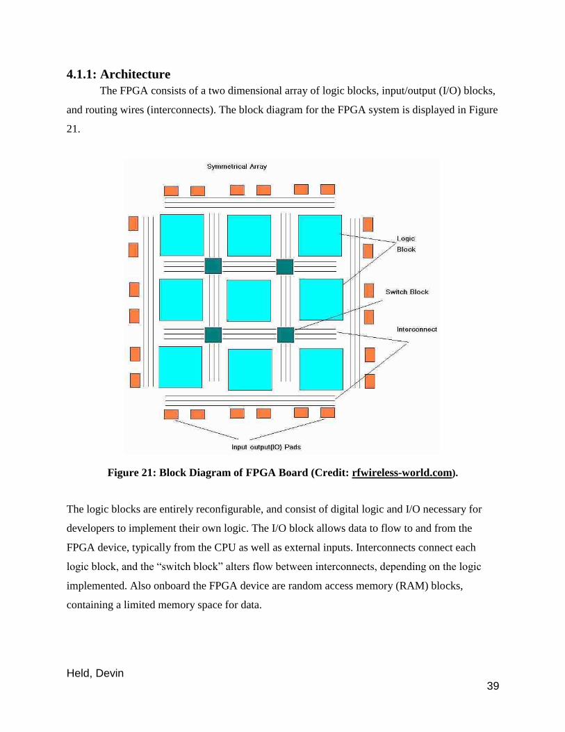
Held, Devin 39

4.1.1: Architecture

The FPGA consists of a two dimensional array of logic blocks, input/output (I/O) blocks,

and routing wires (interconnects). The block diagram for the FPGA system is displayed in Figure

21.

Figure 21: Block Diagram of FPGA Board (Credit: rfwireless-world.com).

The logic blocks are entirely reconfigurable, and consist of digital logic and I/O necessary for

developers to implement their own logic. The I/O block allows data to flow to and from the

FPGA device, typically from the CPU as well as external inputs. Interconnects connect each

logic block, and the “switch block” alters flow between interconnects, depending on the logic

implemented. Also onboard the FPGA device are random access memory (RAM) blocks,

containing a limited memory space for data.

http://rfwireless-world.com/

Held, Devin 40

4.1.2: Development Process

The development process varies for FPGAs, depending on which implementation

language is chosen. For languages such as VHDL and Verilog, circuits must be designed prior to

writing code. In languages such as CUDA or OpenCL, the developer must first decide what will

run on the hardware device and design kernels for each functional aspect. We will focus on the

OpenCL development process as the OpenCL language abstracts away the circuit design aspects,

and this thesis works with OpenCL to implement the CT image reconstruction algorithm. We

will further focus on Altera’s design process as design flow varies from manufacturer to

manufacturer.

First off, the programmer must make design decisions regarding which sections of code

are to be run on the device and on the host, so effective kernels can be programmed. Once code

is written and is ready to be tested, it needs to be run through an emulator to debug errors. This

emulator allows quick compilation of device code, so refactoring written code is not a time

consuming process. After debugging, the code can then be compiled to run on a FPGA. Device

code can be compiled offline to be loaded into the main script, and can take hours to compile.

This long compilation time involves designing the circuits, but takes most time to route the

OpenCL kernels onto the integrated circuit, as effectively designing and placing the circuits is a

complicated task. A virtual FPGA device, an emulator, is used to debug for this reason - the

developer does not want to wait hours to realize their code does not work on a real FPGA. The

emulator runs significantly more slowly than the actual FPGA chip during run time. The offline-

compiled kernels load onto the FPGA at runtime in next to no time, allowing code to be executed

smoothly.

4.1.3: Comparison with GPU and ASICS

Graphics processing units (GPUs) are often built into the average computer nowadays,

making them a cost effective solution to speeding up algorithms. Higher power GPUs can be

purchased to further improve performance, but they can become costly. However, the price

doesn’t come close to the cost of higher tier FPGAs like the Stratix V Chip. GPUs were initially

designed to work with streaming floating point computations, and are therefore a great fit for

image processing applications. GPUs execute instructions in software, which require loading and

queuing instructions prior to executing operations [28]. This is unlike the FPGA, which runs

everything directly on the hardware. Both the GPU and FPGA have great parallel capabilities,

Held, Devin 41

allowing algorithms to developed using efficient multithreading. They both are reconfigurable

devices with no need to scrap any hardware when modifying algorithmic implementations.

However, the development time for the FPGA is considerably longer, as it can take hours for the

compiler to map the code onto logic blocks on the FPGA.

Application-specific integrated circuits (ASICs) are similar to FPGAs as they are

application specific hardware devices used for accelerating computations. However, FPGAs can

be reconfigured at any time, while ASICs require the building of new hardware in order to

modify the underlying processing. This reconfiguration property gives FPGAs an appealing

advantage over the ASICs, as hardware specification may change over time, and it may be costly

to update the ASIC hardware. However, in terms of speed and efficiency, the FPGA and ASIC

devices produce similar energy efficiency and speed performance for algorithms implemented on

same sized chips [27].

There is no definite answer regarding whether GPUs, FPGAs, or ASICs are better - it all

depends on cost, application, and what the device needs to do. There are certainly algorithms

which run better on certain hardware devices. Image processing algorithms tend to run better on

the GPU because of intensive data movement operations due to the size of images being

processed. Algorithms which have performance that could benefit from pipelining and

optimizing circuits are better suited for FPGAs and ASICs. Memory transfer can be a

bothersome bottleneck for algorithms implemented on the FPGA, but IBM has released the

Power8 technology which aims to ease the memory transfer process.

4.2 Power8 Technology

IBM’s Power8 technology is a part of the Power server family, and is a high-performance

processor, providing scalable performance for servers based on the cloud [30,31]. The technical

details of the chip are outlined in IBM’s Power8 slides in Figure 22.

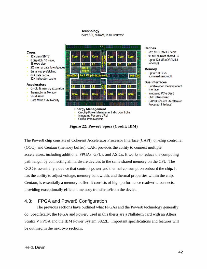
Held, Devin 42

Figure 22: Power8 Specs (Credit: IBM)

The Power8 chip consists of Coherent Accelerator Processor Interface (CAPI), on-chip controller

(OCC), and Centaur (memory buffer). CAPI provides the ability to connect multiple

accelerators, including additional FPGAs, GPUs, and ASICs. It works to reduce the computing

path length by connecting all hardware devices to the same shared memory on the CPU. The

OCC is essentially a device that controls power and thermal consumption onboard the chip. It

has the ability to adjust voltage, memory bandwidth, and thermal properties within the chip.

Centaur, is essentially a memory buffer. It consists of high performance read/write connects,

providing exceptionally efficient memory transfer to/from the device.

4.3: FPGA and Power8 Configuration

The previous sections have outlined what FPGAs and the Power8 technology generally

do. Specifically, the FPGA and Power8 used in this thesis are a Nallatech card with an Altera

Stratix V FPGA and the IBM Power System S822L. Important specifications and features will

be outlined in the next two sections.

Held, Devin 43

4.3.1: Nallatech Card with Altera Stratix V FPGA

The Altera Stratix V FPGA features transceivers up to approximately 28 Gbps,

programmable power management, ethernet capability, and efficient DSP blocks [34]. Altera

states that, “the Stratix V FPGAs deliver the industry’s highest bandwidth, highest level of

system integration, and ultimate flexibility with reduced cost and the lowest total power for high-

end applications” [34]. This high performance card is attached to a Nallatech card, PCIe-385N,

in the system. The Nallatech card key features are a 8-lane PCI Express 3.0 host interface, 2 10G

ethernet channels, and 2 banks of 8 GB SDRAMS [33]. The design of the Nallatech card

focuses on minimizing power consumption, and board size. This card is inserted into the IBM

Power System S822L with the Power8 Processing Technology described in the next section.

4.3.2: IBM Power System S822L

The IBM Power System S822L is a Linux server, optimized for Big Data and cloud

computing [30]. The Power8 processors provide the ability to transfer data more quickly, and

achieve greater efficiency through multithreaded applications. In this context, the key

characteristic of the Power8 is the Centaur and the ability to transfer memory effectively. The

bottleneck of running 3D cone-beam CT reconstruction on an accelerator is the need to transfer

data to and from the CPU. However, with Centaur, this bottleneck has the possibility of being

eliminated due to memory transfer running at 9.6 GB/s [30]. CAPI is also interesting as it allows

the accelerator to use the same shared memory on the CPU, possibly limiting data transfer

entirely.

Held, Devin 44

Chapter 5

5 Benchmarking and Results The algorithm of focus, the Feldkamp, Davis, and Kress (FDK) algorithm for 3D cone-

beam CT image reconstruction, essentially filters and reconstructs a 3D image volume from 2D

projections. The filtering process reduces visual imperfections in the images, called artifacts,

through image processing algorithms such as Ramp Filtering. The back projection process builds

a three dimensional image from the two dimensional x-ray projections, allowing radiologists to

analyze the CT scan in more detail through medical imaging software. Details of this algorithm

are discussed in Chapter 3.

The bottlenecks of the FDK algorithm, memory transfer and computationally intensive

back projection, cause CPU implementations to run very inefficiently. Thus, the move to

accelerators such as graphic processing units (GPUs) and field programmable gate arrays

(FPGAs) provides exponential algorithmic speedups. The parallel nature of both the accelerators

and the FDK algorithm allow developers to write code able to process a large portion of data

across many simultaneous threads. This in turn results in drastic speedups as seen in related

works surveyed in Chapter 2 [sources here].

Much research on speeding up the FDK algorithm focuses on CUDA implementations on

the GPU. There are limited implementations in OpenCL, one of which by Wang et al. [18] was

surveyed in Chapter 2. The use of FPGAs to accelerate this image processing problem is almost

nonexistent. Therefore, it is interesting to experiment with a parallelized approach to

implementing the FDK algorithm to run on a FPGA, reducing the back projection bottleneck.

The use of IBM's Power8 processing technology is nonexistent in this area of research. With

such technology, the memory bottleneck can be approached and possibly eliminated.

The following sections will outline an OpenCL implementation of the FDK algorithm for

a FPGA with Power8 processing technology. The implementation will be benchmarked on the

FPGA,as well as workstation GPU with help from the CPU, and pure CPU. This speed

comparison will give us an idea whether the FPGA is a viable solution to the algorithm's

bottlenecks or not.

Held, Devin 45

5.1: OpenCL

The Open Computing Language (OpenCL) is a framework maintained by Khronos

(www.khronos.org) used for writing heterogenous programs,which run on a mixture of the CPU

and accelerators. Such accelerators consist of GPUs, FPGAs, DSPs, and more. With its basis in

C++, it allows designers to write code for hardware accelerators with little knowledge of circuit

pipelines. Hardware definition languages, such as VHDL, are expensive to write

implementations due to the intense initial learning curve to begin development.

With a clear API for C and C++, developers can easily control what code runs on the

accelerator and when to launch said code. Functions, called kernels, are written to specify code

which will run on the accelerator. Since the kernels are typically compiled at run time, they can

run across a variety of devices with the same implementation. The parallel nature of OpenCL

harnesses the multithreading power of accelerators, thus parallelizing algorithms to their full

potential. Developers have full control of data flow to and from the accelerator, allowing

customization for individual purposes. Unlike CUDA which is built for NVIDIA GPUs, OpenCL

can be used to implement algorithms on various devices, providing lower development costs and

flexibility.

5.1.1: Altera SDK for OpenCL

The Altera SDK for OpenCL provides an easy alternative to an HDL language for

implementing algorithms to run on FPGAs. As mentioned before, writing code for the FPGA

once required circuit design, which proved to be time consuming and difficult. This higher level

approach abstracts away the traditional FPGA design process, simplifying and speeding up

development times.

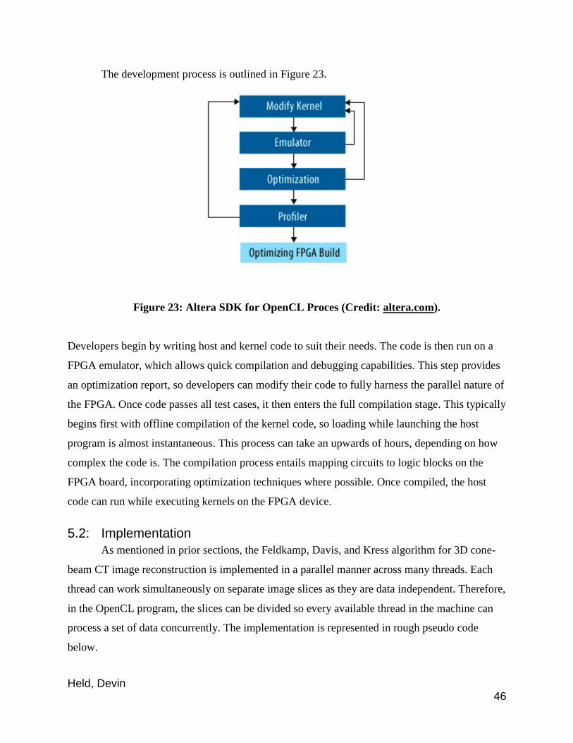
Held, Devin 46

The development process is outlined in Figure 23.

Figure 23: Altera SDK for OpenCL Proces (Credit: altera.com).

Developers begin by writing host and kernel code to suit their needs. The code is then run on a

FPGA emulator, which allows quick compilation and debugging capabilities. This step provides

an optimization report, so developers can modify their code to fully harness the parallel nature of

the FPGA. Once code passes all test cases, it then enters the full compilation stage. This typically

begins first with offline compilation of the kernel code, so loading while launching the host

program is almost instantaneous. This process can take an upwards of hours, depending on how

complex the code is. The compilation process entails mapping circuits to logic blocks on the

FPGA board, incorporating optimization techniques where possible. Once compiled, the host

code can run while executing kernels on the FPGA device.

5.2: Implementation

As mentioned in prior sections, the Feldkamp, Davis, and Kress algorithm for 3D cone-

beam CT image reconstruction is implemented in a parallel manner across many threads. Each

thread can work simultaneously on separate image slices as they are data independent. Therefore,

in the OpenCL program, the slices can be divided so every available thread in the machine can

process a set of data concurrently. The implementation is represented in rough pseudo code

below.

http://altera.com/

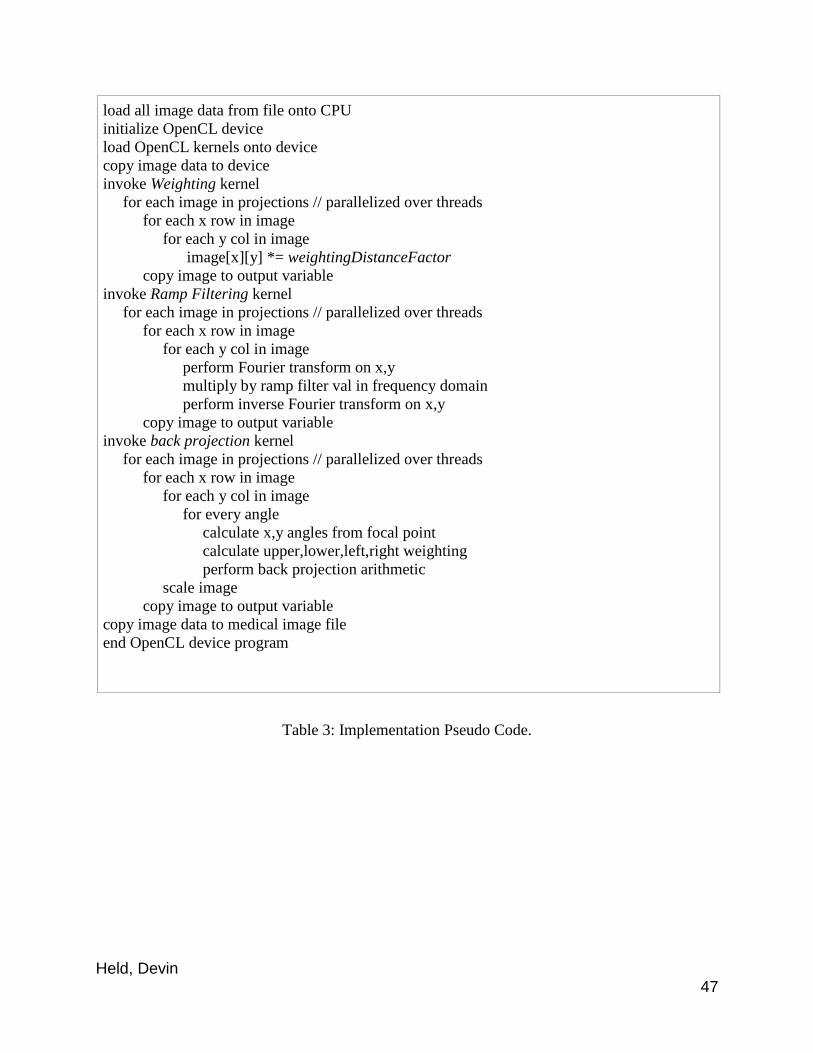
Held, Devin 47

load all image data from file onto CPU

initialize OpenCL device

load OpenCL kernels onto device

copy image data to device

invoke Weighting kernel

for each image in projections // parallelized over threads

for each x row in image

for each y col in image

image[x][y] *= weightingDistanceFactor

copy image to output variable

invoke Ramp Filtering kernel




perform Fourier transform on x,y

multiply by ramp filter val in frequency domain

perform inverse Fourier transform on x,y


invoke back projection kernel




for every angle

calculate x,y angles from focal point

calculate upper,lower,left,right weighting

perform back projection arithmetic

scale image


copy image data to medical image file

end OpenCL device program

Table 3: Implementation Pseudo Code.

Held, Devin 48

5.3: Benchmarking

To test the effectiveness of the OpenCL FPGA implementation, benchmarking was done

across multiple test beds. The comparison between FPGA, GPU, and CPU run times will provide

insight into whether implementing the FDK algorithm in OpenCL for the FPGA is a viable

solution for reducing performance bottlenecks. However, performance varies between different

CPUs, GPUs, and FPGAs. The GPU has already proven to provide immense speedups compared

to CPU implementations [16,17,18,19], but we are focusing on how the FPGA handles such an

algorithm.

5.3.1: Test Beds

Test beds chosen include built in GPU and CPU in an Apple iMac (late 2015) and a

Nallatech FPGA card attached to IBM's S822L power processor. As mentioned before, the focus

is not on the GPU run times, so a workstation desktop computer provides sufficient data for

comparison to the FPGA run time. It is also interesting to discover how the high-tier FPGA runs

the algorithm in comparison to low model GPU, which is optimized for streaming floating point

computations. If the FPGA outperforms the low model GPU, tests could continue on a higher

model GPU. Among the challenges with comparing performance across CPUs, GPUs, and

FPGAs is the difference in architecture. Each device is built to optimize different tasks, thus

operations may perform better on one device in comparison to another. With programming in

OpenCL, the actual circuit routing is hidden from the developer. There is a possibility that

manual designing may provide better solutions than the underlying algorithms in the compiler.

However, it is interesting to explore the difference in performance timings between the different

architectures.

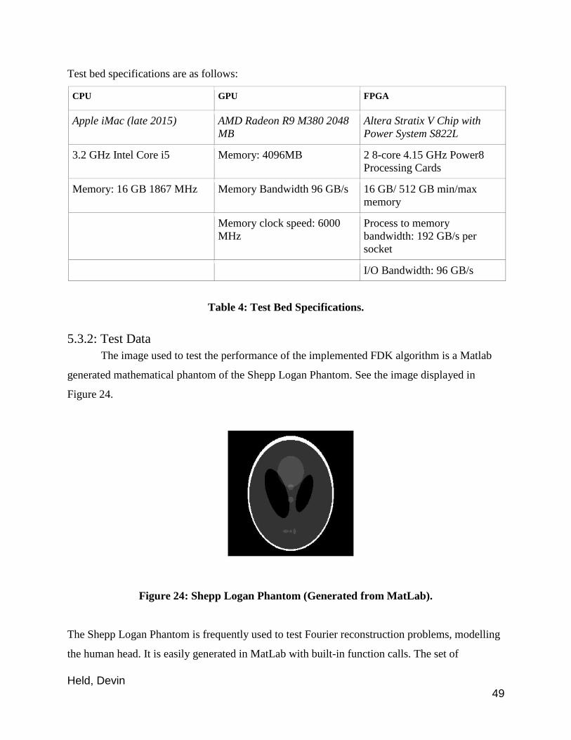
Held, Devin 49

Test bed specifications are as follows:

CPU GPU FPGA

Apple iMac (late 2015) AMD Radeon R9 M380 2048

MB

Altera Stratix V Chip with

Power System S822L

3.2 GHz Intel Core i5 Memory: 4096MB 2 8-core 4.15 GHz Power8

Processing Cards

Memory: 16 GB 1867 MHz Memory Bandwidth 96 GB/s 16 GB/ 512 GB min/max

memory

Memory clock speed: 6000

MHz

Process to memory

bandwidth: 192 GB/s per

socket

I/O Bandwidth: 96 GB/s

Table 4: Test Bed Specifications.

5.3.2: Test Data

The image used to test the performance of the implemented FDK algorithm is a Matlab

generated mathematical phantom of the Shepp Logan Phantom. See the image displayed in

Figure 24.

Figure 24: Shepp Logan Phantom (Generated from MatLab).

The Shepp Logan Phantom is frequently used to test Fourier reconstruction problems, modelling

the human head. It is easily generated in MatLab with built-in function calls. The set of

Held, Devin 50

projections is the sonogram of the phantom, and each individual projection represents two

dimensional slices of the three dimensional image. Two variations of the image were used to test

different data volumes, as CT scans can have a varying sized data sets. However, utilizing a

different image with the same dimensions as the second variation should not make a difference,

as the same amount of computations would incur throughout the reconstruction process. The two

image volumes are described as follows:

1. reconstructs 2563 3D image from 400 projections ;

2. reconstructs 5123 3D image from 600 projections.

Note: The size of the data in the second volume is much larger, and will therefore truly test the

limits of the implementation for the FPGA. The number of projections is a high number for a

general cone-beam CT scanner, and therefore pushes the algorithm to its limits.

5.3.3: Experimental Results

The following tables represent the resulting performance of the OpenCL implementation

of the FDK algorithm on the CPU, GPU, and FPGAs. The three kernels, developed in OpenCL,

will run on the GPU, but are optimized to run on the FPGA. The kernels are timed individually

to demonstrate the lengthy time it requires to run the back projection step in comparison to the

weighting and filtering steps. At the beginning of the main function, a clock_t object is created.

At the end of the function, another clock_t object is created to compute the overall run time.

Individual kernel timers began before initializing any data required for the kernel execution, and

ended after the call to clFinish ended. This allows us to record the time the entire kernel

initialization and execution takes to complete.

The total reconstruction timing also includes reading and writing the image; the results

are averaged over 10 testing sessions. Due to running the exact same code on all devices,

reconstruction image quality did not differ. If implementations varied across platforms, then

slight variations may be present.

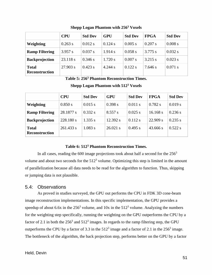
Held, Devin 51

Shepp Logan Phantom with 2563 Voxels

CPU Std Dev GPU Std Dev FPGA Std Dev

Weighting 0.263 s 0.012 s 0.124 s 0.005 s 0.207 s 0.008 s

Ramp Filtering 3.957 s 0.037 s 1.914 s 0.058 s 3.775 s 0.032 s

Backprojection 23.118 s 0.346 s 1.720 s 0.007 s 3.215 s 0.023 s

Total

Reconstruction

27.903 s 0.423 s 4.244 s 0.122 s 7.646 s 0.071 s

Table 5: 2563 Phantom Reconstruction Times.

Shepp Logan Phantom with 5123 Voxels

CPU Std Dev GPU Std Dev FPGA Std Dev

Weighting 0.850 s 0.015 s 0.398 s 0.011 s 0.782 s 0.019 s

Ramp Filtering 28.1877 s 0.332 s 8.557 s 0.025 s 16.168 s 0.236 s

Backprojection 228.180 s 1.335 s 12.392 s 0.112 s 22.909 s 0.235 s

Total

Reconstruction

261.433 s 1.083 s 26.021 s 0.495 s 43.666 s 0.522 s

Table 6: 5123 Phantom Reconstruction Times.

In all cases, reading the 600 image projections took about half a second for the 2563

volume and about two seconds for the 5123 volume. Optimizing this step is limited in the amount

of parallelization because all data needs to be read for the algorithm to function. Thus, skipping

or jumping data is not plausible.

5.4: Observations

As proved in studies surveyed, the GPU out performs the CPU in FDK 3D cone-beam

image reconstruction implementations. In this specific implementation, the GPU provides a

speedup of about 6.6x in the 2563 volume, and 10x in the 5123 volume. Analyzing the numbers

for the weighting step specifically, running the weighting on the GPU outperforms the CPU by a

factor of 2.1 in both the 2563 and 5123 images. In regards to the ramp filtering step, the GPU

outperforms the CPU by a factor of 3.3 in the 5123 image and a factor of 2.1 in the 2563 image.

The bottleneck of the algorithm, the back projection step, performs better on the GPU by a factor

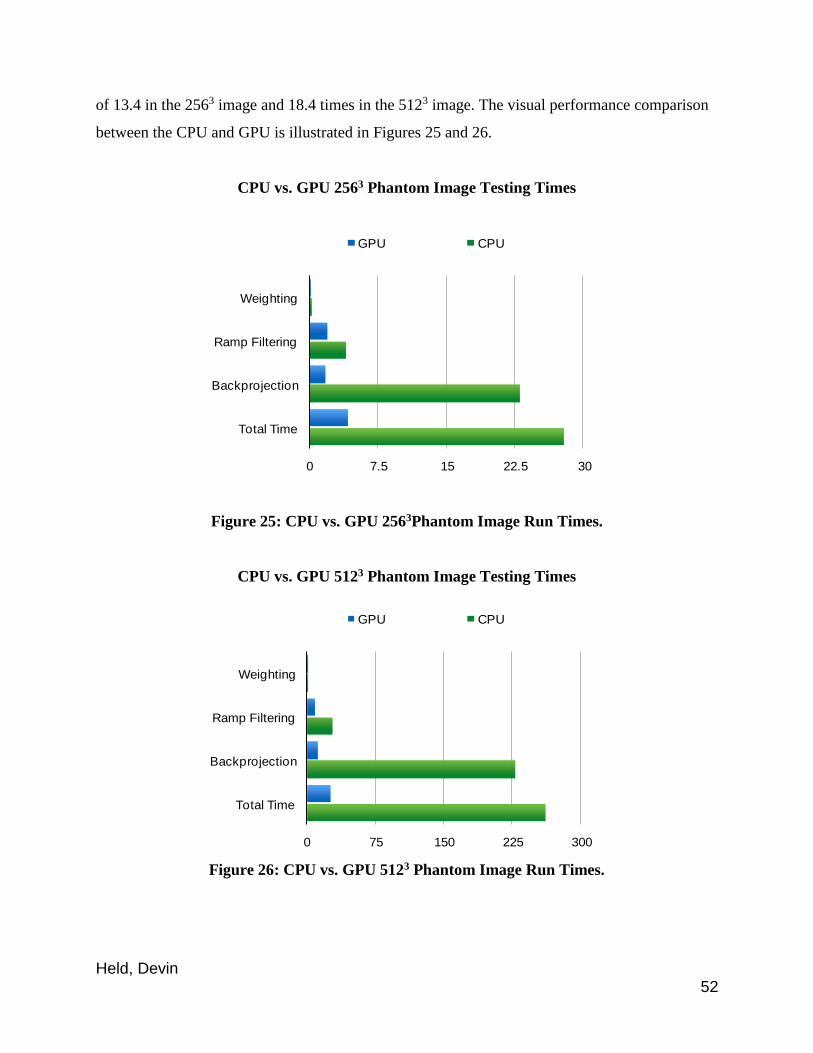
Held, Devin 52

of 13.4 in the 2563 image and 18.4 times in the 5123 image. The visual performance comparison

between the CPU and GPU is illustrated in Figures 25 and 26.

CPU vs. GPU 2563 Phantom Image Testing Times

Figure 25: CPU vs. GPU 2563Phantom Image Run Times.

CPU vs. GPU 5123 Phantom Image Testing Times

Figure 26: CPU vs. GPU 5123 Phantom Image Run Times.

0 7.5 15 22.5 30

Weighting

Ramp Filtering

Backprojection

Total Time

GPU CPU

0 75 150 225 300

Weighting

Ramp Filtering

Backprojection

Total Time

GPU CPU

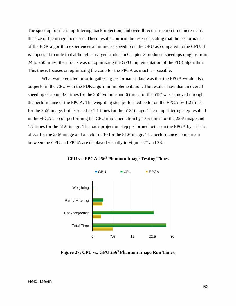
Held, Devin 53

The speedup for the ramp filtering, backprojection, and overall reconstruction time increase as

the size of the image increased. These results confirm the research stating that the performance

of the FDK algorithm experiences an immense speedup on the GPU as compared to the CPU. It

is important to note that although surveyed studies in Chapter 2 produced speedups ranging from

24 to 250 times, their focus was on optimizing the GPU implementation of the FDK algorithm.

This thesis focuses on optimizing the code for the FPGA as much as possible.

What was predicted prior to gathering performance data was that the FPGA would also

outperform the CPU with the FDK algorithm implementation. The results show that an overall

speed up of about 3.6 times for the 2563 volume and 6 times for the 5123 was achieved through

the performance of the FPGA. The weighting step performed better on the FPGA by 1.2 times

for the 2563 image, but lessened to 1.1 times for the 5123 image. The ramp filtering step resulted

in the FPGA also outperforming the CPU implementation by 1.05 times for the 2563 image and

1.7 times for the 5123 image. The back projection step performed better on the FPGA by a factor

of 7.2 for the 2563 image and a factor of 10 for the 5123 image. The performance comparison

between the CPU and FPGA are displayed visually in Figures 27 and 28.

CPU vs. FPGA 2563 Phantom Image Testing Times


0 7.5 15 22.5 30

Weighting

Ramp Filtering

Backprojection

Total Time

GPU CPU FPGA

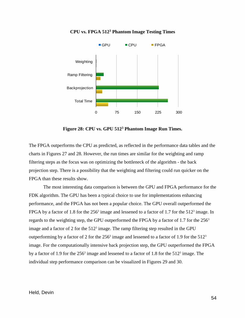
Held, Devin 54

CPU vs. FPGA 5123 Phantom Image Testing Times


The FPGA outperforms the CPU as predicted, as reflected in the performance data tables and the

charts in Figures 27 and 28. However, the run times are similar for the weighting and ramp

filtering steps as the focus was on optimizing the bottleneck of the algorithm - the back

projection step. There is a possibility that the weighting and filtering could run quicker on the

FPGA than these results show.

The most interesting data comparison is between the GPU and FPGA performance for the

FDK algorithm. The GPU has been a typical choice to use for implementations enhancing

performance, and the FPGA has not been a popular choice. The GPU overall outperformed the

FPGA by a factor of 1.8 for the 2563 image and lessened to a factor of 1.7 for the 5123 image. In

regards to the weighting step, the GPU outperformed the FPGA by a factor of 1.7 for the 2563

image and a factor of 2 for the 5123 image. The ramp filtering step resulted in the GPU

outperforming by a factor of 2 for the 2563 image and lessened to a factor of 1.9 for the 5123

image. For the computationally intensive back projection step, the GPU outperformed the FPGA

by a factor of 1.9 for the 2563 image and lessened to a factor of 1.8 for the 5123 image. The

individual step performance comparison can be visualized in Figures 29 and 30.

0 75 150 225 300

Weighting

Ramp Filtering

Backprojection

Total Time

GPU CPU FPGA

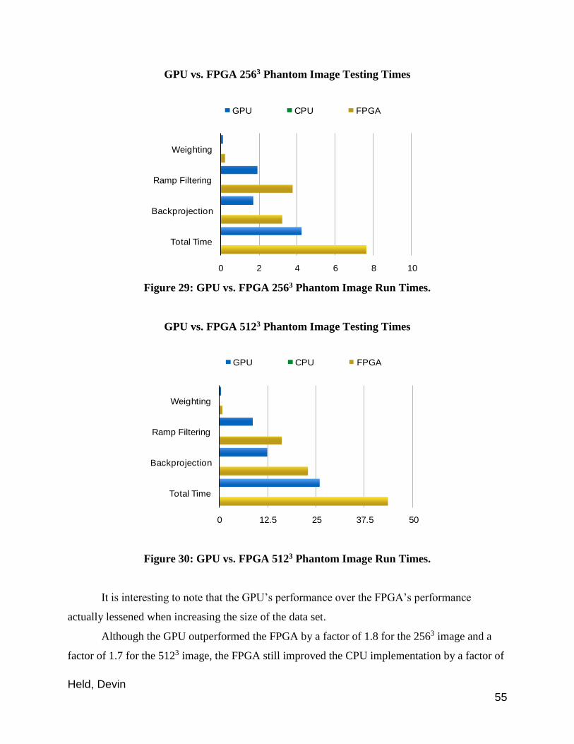
Held, Devin 55

GPU vs. FPGA 2563 Phantom Image Testing Times

Figure 29: GPU vs. FPGA 2563 Phantom Image Run Times.

GPU vs. FPGA 5123 Phantom Image Testing Times

Figure 30: GPU vs. FPGA 5123 Phantom Image Run Times.

It is interesting to note that the GPU’s performance over the FPGA’s performance

actually lessened when increasing the size of the data set.

Although the GPU outperformed the FPGA by a factor of 1.8 for the 2563 image and a

factor of 1.7 for the 5123 image, the FPGA still improved the CPU implementation by a factor of

0 2 4 6 8 10

Weighting

Ramp Filtering

Backprojection

Total Time

GPU CPU FPGA

0 12.5 25 37.5 50

Weighting

Ramp Filtering

Backprojection

Total Time

GPU CPU FPGA

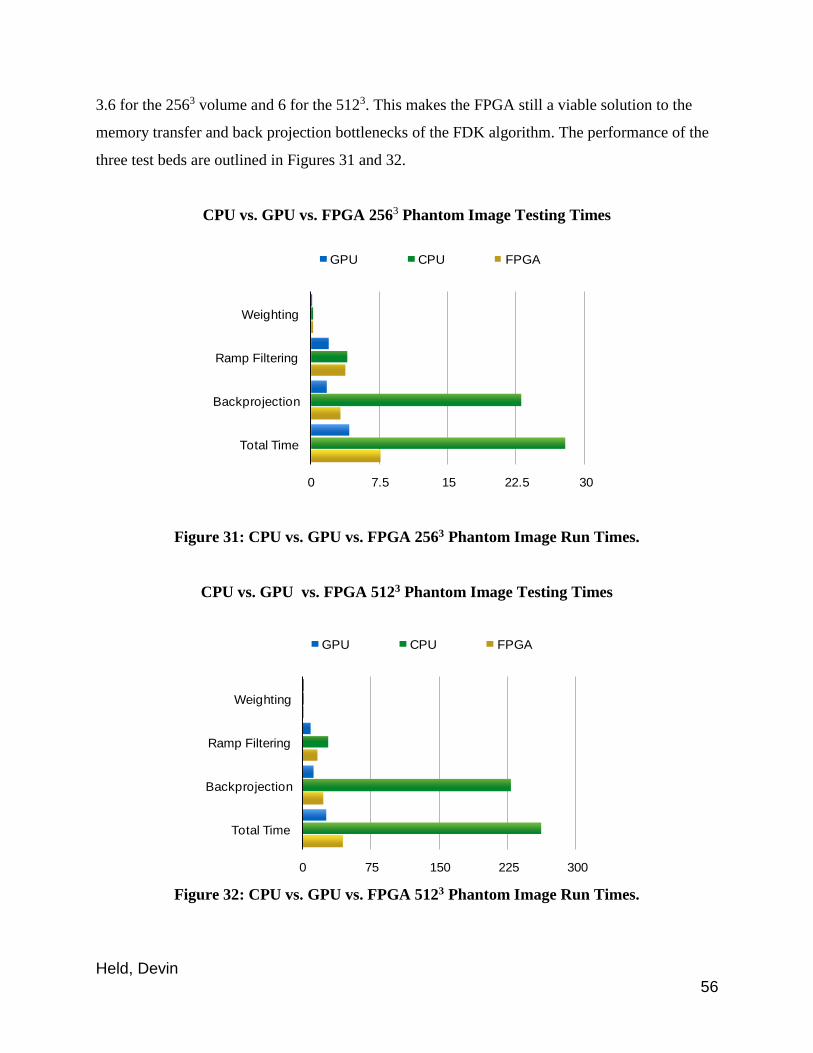
Held, Devin 56

3.6 for the 2563 volume and 6 for the 5123. This makes the FPGA still a viable solution to the

memory transfer and back projection bottlenecks of the FDK algorithm. The performance of the

three test beds are outlined in Figures 31 and 32.

CPU vs. GPU vs. FPGA 2563 Phantom Image Testing Times

Figure 31: CPU vs. GPU vs. FPGA 2563 Phantom Image Run Times.

CPU vs. GPU vs. FPGA 5123 Phantom Image Testing Times

Figure 32: CPU vs. GPU vs. FPGA 5123 Phantom Image Run Times.

0 7.5 15 22.5 30

Weighting

Ramp Filtering

Backprojection

Total Time

GPU CPU FPGA

0 75 150 225 300

Weighting

Ramp Filtering

Backprojection

Total Time

GPU CPU FPGA

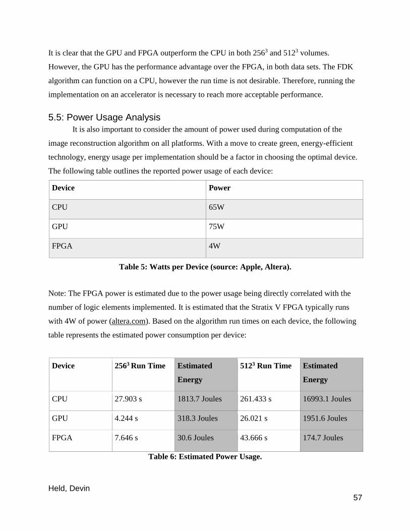
Held, Devin 57

It is clear that the GPU and FPGA outperform the CPU in both 2563 and 5123 volumes.

However, the GPU has the performance advantage over the FPGA, in both data sets. The FDK

algorithm can function on a CPU, however the run time is not desirable. Therefore, running the

implementation on an accelerator is necessary to reach more acceptable performance.

5.5: Power Usage Analysis

It is also important to consider the amount of power used during computation of the

image reconstruction algorithm on all platforms. With a move to create green, energy-efficient

technology, energy usage per implementation should be a factor in choosing the optimal device.

The following table outlines the reported power usage of each device:

Device Power

CPU 65W

GPU 75W

FPGA 4W

Table 5: Watts per Device (source: Apple, Altera).

Note: The FPGA power is estimated due to the power usage being directly correlated with the

number of logic elements implemented. It is estimated that the Stratix V FPGA typically runs

with 4W of power (altera.com). Based on the algorithm run times on each device, the following

table represents the estimated power consumption per device:

Device 2563 Run Time Estimated

Energy

5123 Run Time Estimated

Energy

CPU 27.903 s 1813.7 Joules 261.433 s 16993.1 Joules

GPU 4.244 s 318.3 Joules 26.021 s 1951.6 Joules

FPGA 7.646 s 30.6 Joules 43.666 s 174.7 Joules

Table 6: Estimated Power Usage.

http://altera.com/

Held, Devin 58

Based on these numbers, the FPGA is estimated to run the most energy-efficient

implementation of the FDK algorithm. The time consuming CPU implementation uses the most

energy, while the quickest GPU implementation runs with about 10.6x more power with the 2563

image and 11.2x more power with the 5123 image.

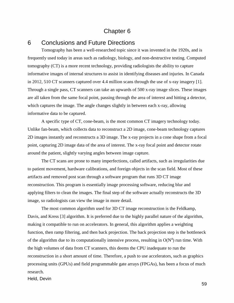
Held, Devin 59

Chapter 6

6 Conclusions and Future Directions Tomography has been a well-researched topic since it was invented in the 1920s, and is

frequently used today in areas such as radiology, biology, and non-destructive testing. Computed

tomography (CT) is a more recent technology, providing radiologists the ability to capture

informative images of internal structures to assist in identifying diseases and injuries. In Canada

in 2012, 510 CT scanners captured over 4.4 million scans through the use of x-ray imagery [1].

Through a single pass, CT scanners can take an upwards of 500 x-ray image slices. These images

are all taken from the same focal point, passing through the area of interest and hitting a detector,

which captures the image. The angle changes slightly in between each x-ray, allowing

informative data to be captured.

A specific type of CT, cone-beam, is the most common CT imagery technology today.

Unlike fan-beam, which collects data to reconstruct a 2D image, cone-beam technology captures

2D images instantly and reconstructs a 3D image. The x-ray projects in a cone shape from a focal

point, capturing 2D image data of the area of interest. The x-ray focal point and detector rotate

around the patient, slightly varying angles between image capture.

The CT scans are prone to many imperfections, called artifacts, such as irregularities due

to patient movement, hardware calibrations, and foreign objects in the scan field. Most of these

artifacts and removed post scan through a software program that runs 3D CT image

reconstruction. This program is essentially image processing software, reducing blur and

applying filters to clean the images. The final step of the software actually reconstructs the 3D

image, so radiologists can view the image in more detail.

The most common algorithm used for 3D CT image reconstruction is the Feldkamp,

Davis, and Kress [3] algorithm. It is preferred due to the highly parallel nature of the algorithm,

making it compatible to run on accelerators. In general, this algorithm applies a weighting

function, then ramp filtering, and then back projection. The back projection step is the bottleneck

of the algorithm due to its computationally intensive process, resulting in O(N4) run time. With

the high volumes of data from CT scanners, this deems the CPU inadequate to run the

reconstruction in a short amount of time. Therefore, a push to use accelerators, such as graphics

processing units (GPUs) and field programmable gate arrays (FPGAs), has been a focus of much

research.

Held, Devin 60

Research on speeding up the algorithm with GPUs has been done very frequently, such as

[16,17,18]. In all cases, researchers found immense speedups in the algorithm if running on a

GPU. Speedups from 25 to 250 times allow us to conclude that the GPU definitely outperforms

the CPU for these computations. What hasn't been investigated is the use of OpenCL on FPGAs

to provide desirable speedups to the algorithm. This thesis focuses on implementing the

algorithm on an FPGA, and comparing the results with the run times from both the CPU and

GPU. With the use of Power8 technology, this thesis further tries to reduce run time by

improving data transfer to and from the accelerator.

6.1: Conclusions

The results in Chapter 5 show a 6 times speedup in computation time when

reconstructing a high quality, 5123 image on the FPGA compared to the CPU. The FPGA excels

in the back projection step, outperforming the CPU by a factor of 10. It is also interesting to note

that the FPGA runs the implementation in slower time, but is 10-11x more energy efficient.

These results indicate that the FPGA is a viable solution to speeding up this algorithm.

However, when compared with the run times on the GPU, the GPU outperforms the

FPGA by a factor of 1.7. The backprojection step runs about 10 seconds faster on the GPU. The

GPU not only provides great speedups, but it is much more easily available to the public. GPUs

are built into many workstation desktops, so medical personnel are not required to purchase an

additional accelerator, unless of course they wish to add a more powerful device. The cost of a

FPGA can range from $2000-$15000 CAD (buyaltera.com). This cost doesn't cover the high-

power workstation desktop required to install the necessary components and communicate with

the accelerator. The Power8 technology can range from $8000-$18000 (ibm.com). Therefore,

such a system to run the FPGA with Power8 implementation could cost an upwards of $50000.

However, the Power8 technology is not a necessity to run the implementation on a FPGA,

reducing cost dramatically. Also, of course, these devices drop in price over time, further

reducing cost to run such an implementation.

Due to the low cost and quick implementation, the GPU appears to be a better approach

than the FPGA to improve run time of the FDK algorithm. The GPU in this thesis provided a 10

times speedup from the CPU implementation for the high-quality image. These numbers have the

potential to drastically improve if tested with a higher-power GPU or if time was spent

optimizing the code for the GPU implementation rather than for the FPGA. GPUs are cheap in

Held, Devin 61

comparison to the FPGA, and they run the FDK algorithm quicker than the FPGA. Although

both devices provide great speedups, the GPU would be a better option to run 3D cone-beam CT

image reconstruction.

6.2: Future Directions

Another approach to testing the usefulness of the field programmable gate array (FPGA)

for 3D cone-beam CT reconstruction would be to write the implementation in a hardware

programming language such as virtual hardware detection language (VHDL). This would enable

a design and pipeline circuits that are coded onto the accelerator. Using OpenCL to program the

FPGA provides many optimization techniques, but little customization when it comes to circuit

design due to the fact that the OpenCL language abstracts out the circuit design level in the

development process. It is possible to further implement more optimization techniques, further

reducing computation time, but designing the low level circuits is not plausible. The OpenCL

language takes a long time to compile because it is translating the code from C into a hardware

circuit layout to map onto the device. Writing the code at the absolute lowest level will allow all

possible optimization techniques to be implemented, possibly improving the algorithmic run time

on the FPGA.

Another possible future direction could include running the code on a mixture of GPUs

and FPGAs. Work has been done to run the code on multiple GPUs to achieve an even higher

speedup, so the possibility of a GPU and FPGA working together to do calculations on

individual slices could also speedup run time. Different models of FPGAs could be used, as well

as different servers and workstation desktops connected to the FPGA cards.

The Feldkamp, Davis, and Kress (FDK) algorithm for cone-beam image reconstruction is

not the only algorithm designed to reconstruct 3D images. It actually provides an approximate

image reconstruction in comparison to exact reconstructions such as those resulting from

Grangreat's or Katsevich's algorithms. It could be interesting to explore whether one of these

algorithms runs more efficiently on the FPGA in comparison to the GPU.

This paper focuses on the Feldkamp, Davis, and Kress algorithm for 3D cone-beam CT

image reconstruction implemented and optimized for the FPGA. There are many different ways

this problem could be approached to confirm the results found in this paper. As stated above,

there are multiple variations in the approach that could yield varying results. However, based on

Held, Devin 62

results from this thesis, the GPU appears to be a better solution to the 3D CT reconstruction

problem.

Held, Devin 63

References [1] Canadian Institute for Health Information, “Medical Imaging”, www.cihi.ca, Accessed 18

August 2016

[2] National Institute of Biomedical Imaging and Bioengineering, “X-rays”, www.nibib.nih.gov,

Accessed 18 August 2016

[3] Feldkamp, L. A., L. C. Davis, and J. W. Kress. "Practical cone-beam algorithm." JOSA A 1.6

(1984): 612-619.

[4] Physics Central, “CT Scans”, www.physicscentral.com, Accessed 18 August 2016

[5] Webb, Steve. "A brief history of tomography and CT." PROCEEDINGS 7th ASIAN &

OCEANIAN CONGRESS OF RADIOLOGY (1995): 429-431

[6] Seynaeve, P. C., and J. I. Broos. "The History of Tomography" Journal belge de radiologie

78.5 (1995): 284-288.

[7] Barrett, Julia F., and Nicholas Keat. "Artifacts in CT: Recognition and Avoidance 1."

Radiographics 24.6 (2004): 1679-1691.

[8] Ohnesorge, B., et al. "Efficient Correction for CT Image Artifacts Caused by Objects

Extending Outside the Scan Field of View." Medical physics 27.1 (2000): 39-46.

[9] Jamieson, Peter, et al. "An Energy and Power Consumption Analysis of FPGA Routing

Architectures." Field-Programmable Technology (2009): 324-327

[10] Gengsheng L, Zeng et al. “Fan-Beam Reconstruction Algorithm for a Spatially Varying

Focal Length Collimator” IEEE Transactions on Medical Imaging 12.3 (1993): 575-582

[11] Zeng, Gengsheng Lawrence. “Medical Image Reconstruction” Heidelberg: Springer (2010)

[12] Sedentexct, “Technical Description of CBCT”, www.sedentexct.eu, Accessed 20 August

2016

[13] Scarfe, William C., and Allan G. Farman. "What is Cone-Beam CT and How Does it

Work?" Dental Clinics of North America 52.4 (2008): 707-730.

[14] Wang, Ge, et al. "A General Cone-Beam Reconstruction Algorithm." IEEE Transactions on

Medical Imaging 12.3 (1993): 486-496.

[15] Zhao, Xing, Jing-jing Hu, and Peng Zhang. "GPU-Based 3D Cone-Beam CT Image

Reconstruction for Large Data Volume." Journal of Biomedical Imaging (2009): 8-9

[16] Okitsu Yusuke, Fumihiko Ino, and Kenichi Hagihara. "High-Performance Cone Beam

Reconstruction using CUDA Compatible GPUs." Parallel Computing 36.2 (2010): 129-141.

http://www.cihi.ca/

http://www.nibib.nih.gov/

http://www.physicscentral.com/

http://www.sedentexct.eu/

Held, Devin 64

[17] Noël, Peter B., et al. "GPU-Based Cone Beam Computed Tomography." Computer Methods

and Programs in Biomedicine 98.3 (2010): 271-277.

[18] Wang, Bo, et al. "Accelerated Cone Beam CT Reconstruction Based on OpenCL."

International Conference on Image Analysis and Signal Processing. IEEE (2010): 291-295

[19] Gac, Nicolas, et al. "High Speed 3D Tomography on CPU, GPU, and FPGA." EURASIP

Journal on Embedded systems 2008 (2008): 5-6

[20] Zeng, Gengsheng Lawrence. “Medical image reconstruction”. Heidelberg: Springer (2010):

55-64

[21] Bevel, “The Fourier Transform”, www.thefouriertransform.com, Accessed 25 August 2016

[22] Rice University, “Backprojection Filters”,

clear.rice.edu/elec431/projects96/DSP/filters.html, Accessed 25 August 2016

[23] Goldman, Lee W. "Principles of CT and CT Technology." Journal of nuclear medicine

technology 35.3 (2007): 115-128.

[24] Source Tech, “Top FPGA Companies for 2013”, www.sourcetech411.com, Accessed 26

August 2016

[25] Wilson, Ron. “In the Beginning”, www.altera.com, Accessed 25 September 2016

[26] Gianelli, Silvia. “Hall of Fame Inductee for Invention of FPGA”, www.press.xilinx.com,

Accessed 25 October 2016

[27] Moore, Andrew. “FPGAs for Dummies”, Wiley (2014): 5-12

[28] Adams, Charlotte. “FPGA GPU Evolution Continues”, www.mil-embedded.com, Accessed

25 October 2016

[29] Mujtaba, Hassan. “IBM Power8 Processor Detailed” (2013) 1-3

[30] IBM, “IBM PowerSystem Mission Statement”, www.IBM.com, Accessed 12 November

2016

[31] Lyra, Maria, and Agapi Ploussi. "Filtering in SPECT image reconstruction." Journal of

Biomedical Imaging 2011 (2011): 10-11

[32] IBM, “Pinned and Non-Pinned Memory”,

http://www.ibm.com/support/knowledgecenter/SSFKCN_3.5.0/com.ibm.cluster.gpfs.v3r5.gpfs3

00.doc/bl1ins_pnonpmem.htm, Accessed 15 November 2016

[33] Nallatech, “385 Hardware Reference Guide”, www.nallatech.com, Accessed 15 November

2016

http://www.thefouriertransform.com/

https://www.clear.rice.edu/elec431/projects96/DSP/filters.html

http://www.sourcetech411.com/

http://www.altera.com/

http://www.press.xilinx.com/

http://www.mil-embedded.com/

http://www.ibm.com/

http://www.ibm.com/support/knowledgecenter/SSFKCN_3.5.0/com.ibm.cluster.gpfs.v3r5.gpfs300.doc/bl1ins_pnonpmem.htm

http://www.ibm.com/support/knowledgecenter/SSFKCN_3.5.0/com.ibm.cluster.gpfs.v3r5.gpfs300.doc/bl1ins_pnonpmem.htm

http://www.nallatech.com/

Held, Devin 65

[34] Altera, “Stratix V”, https://www.altera.com/content/dam/altera-

www/global/en_US/pdfs/literature/hb/stratix-v/stx5_51001.pdf, Accessed 15 November 2016

https://www.altera.com/content/dam/altera-www/global/en_US/pdfs/literature/hb/stratix-v/stx5_51001.pdf

https://www.altera.com/content/dam/altera-www/global/en_US/pdfs/literature/hb/stratix-v/stx5_51001.pdf

Held, Devin 66

Curriculum Vitae

Name: Devin Held

Post-secondary University of Irvine, California

Education and Irvine, California, United States

Degrees: 2012-2015 B.S.

Western University

London, Ontario, Canada

2015-2016 M.Sc.

Honours and Dean’s Honour List

Awards: 2012-2015

Related Work Teaching Assistant and Graduate Researcher

Experience: Western University

2015-2016

Java Development Intern

BookingPal Inc.

2014-2015

Undergraduate Researcher

UC Irvine

2013-2014

Documents

Analysis of 3D Cone-Beam CT Image Reconstruction