Differential Cone-Beam CT Reconstruction for Planar Objectscdn.intechopen.com/pdfs-wm/24027.pdf · Differential Cone-Beam CT Reconstruction for Planar Objects ... Differential Cone-Beam

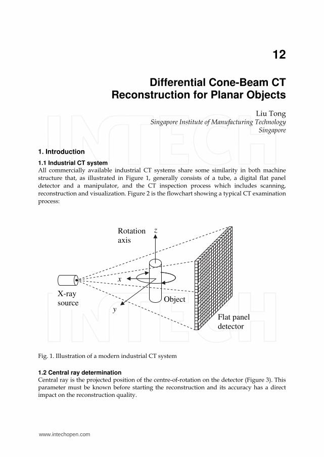
12

Differential Cone-Beam CT Reconstruction for Planar Objects

Liu Tong Singapore Institute of Manufacturing Technology

Singapore

1. Introduction

1.1 Industrial CT system All commercially available industrial CT systems share some similarity in both machine

structure that, as illustrated in Figure 1, generally consists of a tube, a digital flat panel

detector and a manipulator, and the CT inspection process which includes scanning,

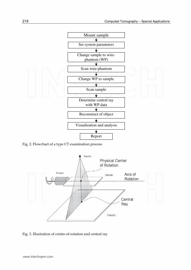
reconstruction and visualization. Figure 2 is the flowchart showing a typical CT examination

process:

Fig. 1. Illustration of a modern industrial CT system

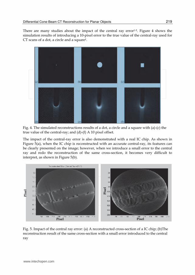
1.2 Central ray determination Central ray is the projected position of the centre-of-rotation on the detector (Figure 3). This parameter must be known before starting the reconstruction and its accuracy has a direct impact on the reconstruction quality.

y

x

z

X-ray

source Object

Flat panel

detector

Rotation

axis

www.intechopen.com

Computed Tomography – Special Applications

218

Fig. 2. Flowchart of a type CT examination process

Fig. 3. Illustration of centre-of-rotation and central ray

Mount sample

Set system parameters

Change sample to wire-

phantom (WP)

Scan wire-phantom

Scan sample

Change WP to sample

Determine central ray

with WP data

Reconstruct of object

Visualization and analysis

Report

www.intechopen.com


219

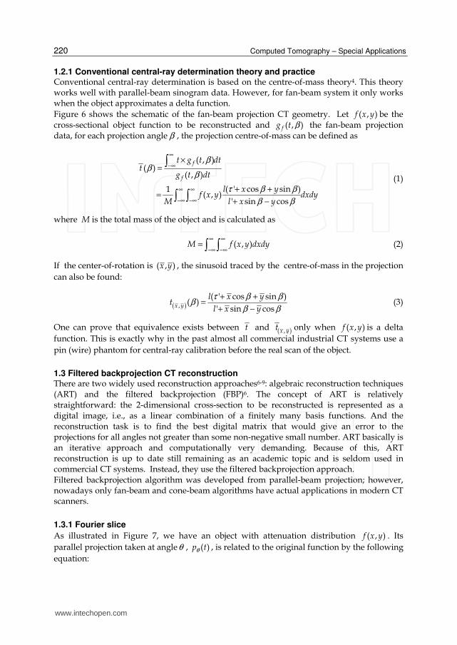
There are many studies about the impact of the central ray error1-5. Figure 4 shows the simulation results of introducing a 10-pixel error to the true value of the central-ray used for CT scans of a dot, a circle and a square1.

Fig. 4. The simulated reconstructions results of a dot, a circle and a square with (a)-(c) the true value of the central-ray; and (d)-(f) A 10 pixel offset.

The impact of the central-ray error is also demonstrated with a real IC chip. As shown in Figure 5(a), when the IC chip is reconstructed with an accurate central-ray, its features can be clearly presented on the image; however, when we introduce a small error to the central ray and redo the reconstruction of the same cross-section, it becomes very difficult to interpret, as shown in Figure 5(b).

Fig. 5. Impact of the central ray error: (a) A reconstructed cross-section of a IC chip; (b)The reconstruction result of the same cross-section with a small error introduced to the central ray

Pixel Pixel

Pix

el

Pix

el

www.intechopen.com


220

1.2.1 Conventional central-ray determination theory and practice Conventional central-ray determination is based on the centre-of-mass theory4. This theory works well with parallel-beam sinogram data. However, for fan-beam system it only works when the object approximates a delta function.

Figure 6 shows the schematic of the fan-beam projection CT geometry. Let ( , )f x y be the cross-sectional object function to be reconstructed and ( , )fg t β the fan-beam projection data, for each projection angle β , the projection centre-of-mass can be defined as

( , )( )

( , )

( ' cos sin )1( , )

' sin cos

f

f

t g t dtt

g t dt

l x yf x y dxdy

M l x y

ββ

β

τ β β

β β

∞

−∞

∞ ∞

−∞ −∞

×=

+ +=

+ −

(1)

where M is the total mass of the object and is calculated as

( , )M f x y dxdy∞ ∞

−∞ −∞= (2)

If the center-of-rotation is ( , )x y , the sinusoid traced by the centre-of-mass in the projection

can also be found:

( ),

( ' cos sin )( )

' sin cosx y

l x yt

l x y

τ β ββ

β β

+ +=

+ − (3)

One can prove that equivalence exists between t and ( ),x yt only when ( , )f x y is a delta

function. This is exactly why in the past almost all commercial industrial CT systems use a

pin (wire) phantom for central-ray calibration before the real scan of the object.

1.3 Filtered backprojection CT reconstruction There are two widely used reconstruction approaches6-9: algebraic reconstruction techniques (ART) and the filtered backprojection (FBP)6. The concept of ART is relatively straightforward: the 2-dimensional cross-section to be reconstructed is represented as a digital image, i.e., as a linear combination of a finitely many basis functions. And the reconstruction task is to find the best digital matrix that would give an error to the projections for all angles not greater than some non-negative small number. ART basically is an iterative approach and computationally very demanding. Because of this, ART reconstruction is up to date still remaining as an academic topic and is seldom used in commercial CT systems. Instead, they use the filtered backprojection approach. Filtered backprojection algorithm was developed from parallel-beam projection; however, nowadays only fan-beam and cone-beam algorithms have actual applications in modern CT scanners.

1.3.1 Fourier slice

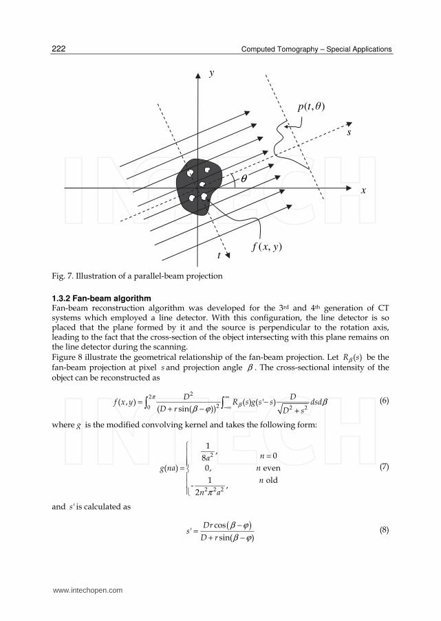
As illustrated in Figure 7, we have an object with attenuation distribution ( , )f x y . Its

parallel projection taken at angleθ , ( )p tθ , is related to the original function by the following

equation:

www.intechopen.com


221

( )

( )( , ) ( , ) ( , ) cos sinp t f s t ds f x y x y t dxdyθ

θ δ θ θ∞ ∞

−∞ −∞= = + − (4)

and inversely, the object density distribution function can be obtained from the measurements of projections by

0

( , ) ( , ) ( ' )m

m

t

tf x y d p t h t t dt

πθ θ

−= − (5)

where ( )h t is convolution kernel, written in discrete form as

( )

2

2

104

( ) 0 even

1 old

n

h n n

n

n

δδ

πδ

=

= −

(6)

Fig. 6. Schematic of fan-beam projection CT geometry

β

'τ

τ

x

y

t

't

),( βtg f

),( yxf

Centre-of-rotation

Central ray

))(( βτ

www.intechopen.com


222

Fig. 7. Illustration of a parallel-beam projection

1.3.2 Fan-beam algorithm Fan-beam reconstruction algorithm was developed for the 3rd and 4th generation of CT systems which employed a line detector. With this configuration, the line detector is so placed that the plane formed by it and the source is perpendicular to the rotation axis, leading to the fact that the cross-section of the object intersecting with this plane remains on the line detector during the scanning. Figure 8 illustrate the geometrical relationship of the fan-beam projection. Let ( )R sβ be the fan-beam projection at pixel s and projection angle β . The cross-sectional intensity of the object can be reconstructed as

2

2

20 2 2( , ) ( ) ( ' )

( sin( ))

D Df x y R s g s s dsd

D r D s

π

β ββ ϕ

∞

−∞= −

+ − + (6)

where g is the modified convolving kernel and takes the following form:

2

2 2 2

1,

08( ) 0, even

1 old- ,

2

nag na n

n

n aπ

==

(7)

and 's is calculated as

( )cos'

sin( )

Drs

D r

β ϕ

β ϕ

−=

+ − (8)

s

t

x

y

),( θtp

),( yxf

θ

www.intechopen.com


223

Fig. 8. Geometrical relationship of a fan-beam projection

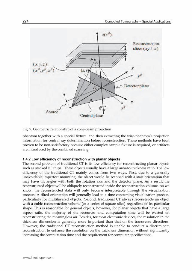
1.3.3 Cone-beam algorithm

Figure 9 illustrates the definitions of the reconstruction slices and the associated coordinate

systems involved in the development of the traditional cone-beam reconstruction algorithm.

With these definitions, any point on the thi slice of the object is calculated as7

2 2 '

2 2 2

1( , , ) ( ) ( , , ) ( )

2 ' ( )

m

mi

D Df x y z d q s v h s s ds

D y D s v

π γ γ β

γ γβ β

−

− −= −

+ + + (9)

where h is the convolving kernel; D is the source-to-object distance, i.e., the distance from

the source to the global coordinate centre; and ( ), ,q s v β is the projection data at pixel ( ),s v

at projection angle β , with ( ),s v being calculated as

cos sin

( sin cos ) i

s x yD

v zD x y

β β

β β

− =

− + (10)

1.4 Two issues with conventional CT inspection 1.4.1 Central ray determination with wire phantom This method simply means that one needs an extra scan just for the determination of the

central ray parameter. This is not only a waste of human and system resources and effort,

but also a cause of uncertainty in the determination of central ray due to the mounting and

dismounting process of the wire-phantom and the object. To minimize the effect of these

problems, many techniques have been developed4, 5. These methods adopt similar ideas of

either integrating the wire-phantom into the rotary system or scanning object and wire-

),(or),( φryx r

φ

Dβ

x

y

Central-ray

S

O

s

www.intechopen.com


224

Fig. 9. Geometric relationship of a cone-beam projection

phantom together with a special fixture and then extracting the wire-phantom’s projection information for central ray determination before reconstruction. These methods have been proven to be non-satisfactory because either complex sample fixture is required, or artifacts are introduced by the combined scanning.

1.4.2 Low efficiency of reconstruction with planar objects The second problem of traditional CT is its low-efficiency for reconstructing planar objects such as stacked IC chips. These objects usually have a large area-to-thickness ratio. The low efficiency of the traditional CT mainly comes from two ways. First, due to a generally unavoidable imperfect mounting, the object would be scanned with a start orientation that may have tilt angles with both the rotation axis and the detector plane. As a result the reconstructed object will be obliquely reconstructed inside the reconstruction volume. As we know, the reconstructed data will only become interpretable through the visualization process. A tilted orientation will generally lead to a time-consuming visualization process, particularly for multilayered objects. Second, traditional CT always reconstructs an object with a cubic reconstruction volume (or a series of square slice) regardless of its particular shape. This is reasonable for general objects, however, for planar objects that have a large aspect ratio, the majority of the resources and computation time will be wasted on reconstructing the meaningless air. Besides, for most electronic devices, the resolution in the thickness dimension is generally more important than that on the transverse directions. However, the traditional CT reconstruction method is unable to conduct a discriminate reconstruction to enhance the resolution on the thickness dimension without significantly increasing the computation time and the requirement for computer specifications.

www.intechopen.com


225

2. Automatic centre determination

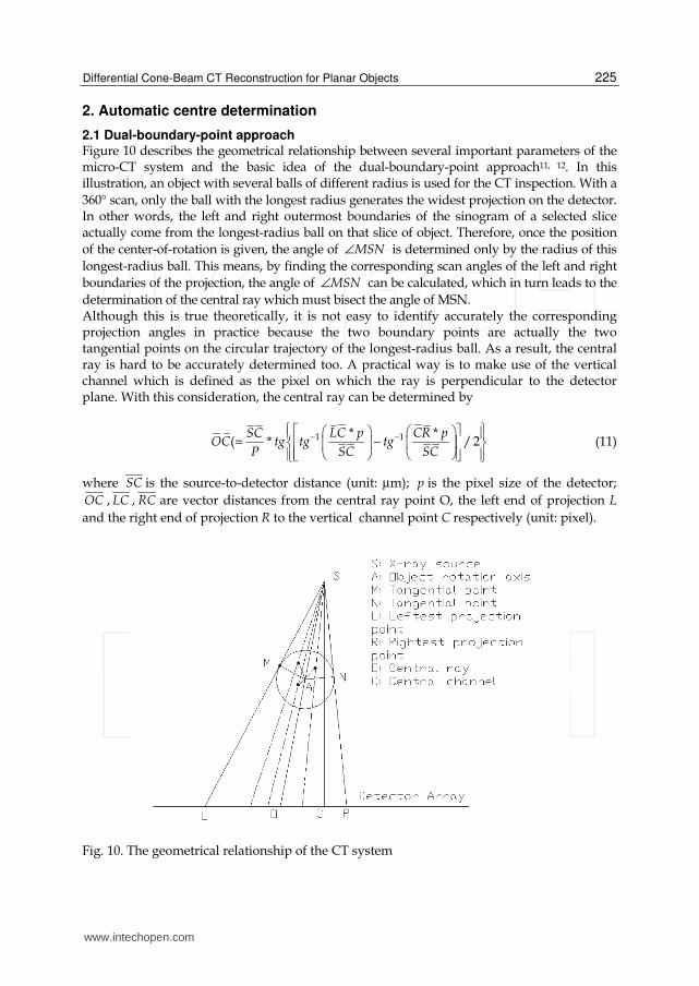
2.1 Dual-boundary-point approach Figure 10 describes the geometrical relationship between several important parameters of the micro-CT system and the basic idea of the dual-boundary-point approach11, 12. In this illustration, an object with several balls of different radius is used for the CT inspection. With a

360° scan, only the ball with the longest radius generates the widest projection on the detector. In other words, the left and right outermost boundaries of the sinogram of a selected slice actually come from the longest-radius ball on that slice of object. Therefore, once the position

of the center-of-rotation is given, the angle of MSN∠ is determined only by the radius of this

longest-radius ball. This means, by finding the corresponding scan angles of the left and right

boundaries of the projection, the angle of MSN∠ can be calculated, which in turn leads to the

determination of the central ray which must bisect the angle of MSN. Although this is true theoretically, it is not easy to identify accurately the corresponding projection angles in practice because the two boundary points are actually the two tangential points on the circular trajectory of the longest-radius ball. As a result, the central ray is hard to be accurately determined too. A practical way is to make use of the vertical channel which is defined as the pixel on which the ray is perpendicular to the detector plane. With this consideration, the central ray can be determined by

1 1* *( * / 2

LC p CR pSCOC tg tg tg

P SC SC− −

= − (11)

where SC is the source-to-detector distance (unit: µm); p is the pixel size of the detector;

OC , LC , RC are vector distances from the central ray point O, the left end of projection L

and the right end of projection R to the vertical channel point C respectively (unit: pixel).

Fig. 10. The geometrical relationship of the CT system

www.intechopen.com


226

The vertical line C is a fixed parameter and only need to be recalibrated when some

movement conducted to the detector in possible system maintenance or detector repair.

If both LC and RC are small compared to SC so that tan x x≈ is true, the central ray can be

simply determined as the center of LR , that is,

1

2LO LC CR= + (12)

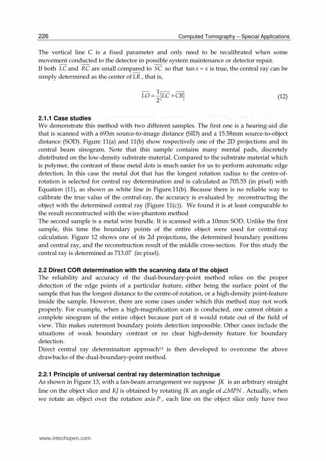
2.1.1 Case studies We demonstrate this method with two different samples. The first one is a hearing-aid die

that is scanned with a 693m source-to-image distance (SID) and a 15.58mm source-to-object

distance (SOD). Figure 11(a) and 11(b) show respectively one of the 2D projections and its

central beam sinogram. Note that this sample contains many mental pads, discretely

distributed on the low-density substrate material. Compared to the substrate material which

is polymer, the contrast of these metal dots is much easier for us to perform automatic edge

detection. In this case the metal dot that has the longest rotation radius to the centre-of-

rotation is selected for central ray determination and is calculated as 705.55 (in pixel) with

Equation (11), as shown as white line in Figure.11(b). Because there is no reliable way to

calibrate the true value of the central-ray, the accuracy is evaluated by reconstructing the

object with the determined central ray (Figure 11(c)). We found it is at least comparable to

the result reconstructed with the wire-phantom method

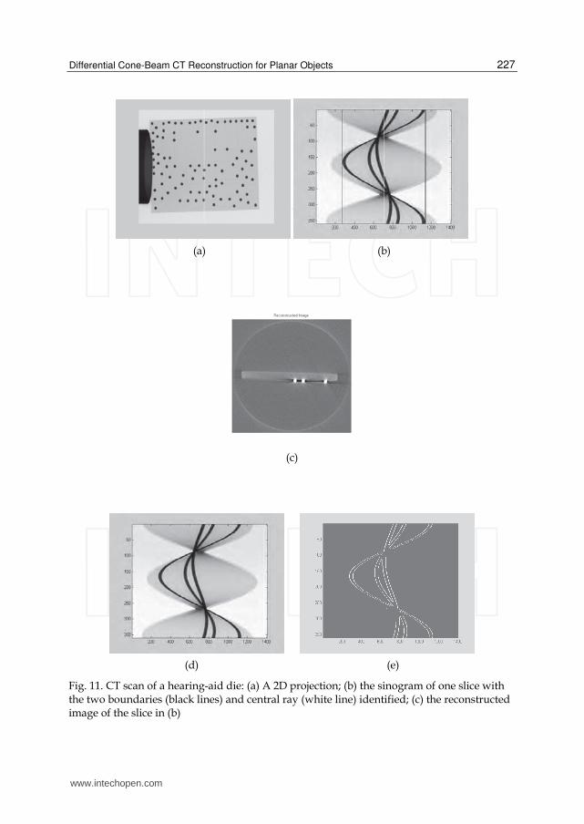
The second sample is a metal wire bundle. It is scanned with a 10mm SOD. Unlike the first

sample, this time the boundary points of the entire object were used for central-ray

calculation. Figure 12 shows one of its 2d projections, the determined boundary positions

and central ray, and the reconstruction result of the middle cross-section. For this study the

central ray is determined as 713.07 (in pixel).

2.2 Direct COR determination with the scanning data of the object The reliability and accuracy of the dual-boundary-point method relies on the proper

detection of the edge points of a particular feature, either being the surface point of the

sample that has the longest distance to the centre-of-rotation, or a high-density point-feature

inside the sample. However, there are some cases under which this method may not work

properly. For example, when a high-magnification scan is conducted, one cannot obtain a

complete sinogram of the entire object because part of it would rotate out of the field of

view. This makes outermost boundary points detection impossible. Other cases include the

situations of weak boundary contrast or no clear high-density feature for boundary

detection.

Direct central ray determination approach13 is then developed to overcome the above

drawbacks of the dual-boundary-point method.

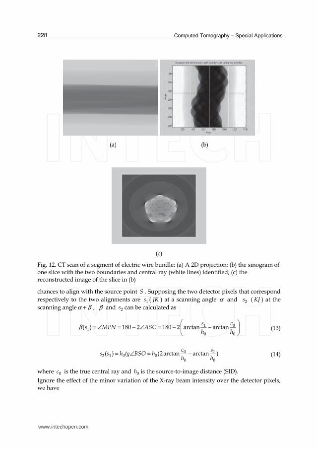
2.2.1 Principle of universal central ray determination technique

As shown in Figure 13, with a fan-beam arrangement we suppose JK is an arbitrary straight

line on the object slice and KJ is obtained by rotating JK an angle of MPN∠ . Actually, when

we rotate an object over the rotation axis P , each line on the object slice only have two

www.intechopen.com


227

(a) (b)

(c)

(d) (e)

Fig. 11. CT scan of a hearing-aid die: (a) A 2D projection; (b) the sinogram of one slice with the two boundaries (black lines) and central ray (white line) identified; (c) the reconstructed image of the slice in (b)

www.intechopen.com


228

(a) (b)

(c)

Fig. 12. CT scan of a segment of electric wire bundle: (a) A 2D projection; (b) the sinogram of one slice with the two boundaries and central ray (white lines) identified; (c) the reconstructed image of the slice in (b)

chances to align with the source point S . Supposing the two detector pixels that correspond

respectively to the two alignments are 1s ( JK ) at a scanning angle α and 2s ( KJ ) at the

scanning angle α β+ , β and 2s can be calculated as

01

10 0

( ) 180 2 180 2 arctan arctancs

s MPN ASCh h

β

= ∠ = − ∠ = − − (13)

0 1

2 1 0 00 0

( ) (2 arctan arctan )c s

s s h tg BSO hh h

= ∠ = − (14)

where 0c is the true central ray and 0h is the source-to-image distance (SID).

Ignore the effect of the minor variation of the X-ray beam intensity over the detector pixels, we have

www.intechopen.com


229

1 2( ) ( )P s P sα α β+= (15)

This property is the basis of our universal fan-beam central ray determination. In the

practical implementation, we can assume a set of central ray values { }ic and for each ic we

calculate 2s and β , and then perform the following measurement

2 2

1

1 1 1

21 ( ) 2 1( ) [ ( ) ( ( ))]

n t

i sn s t

M c P s P s sα α βα

+= =

= − (16)

Obviously M should reach a minimum value when 0ic c= .

Fig. 13. Principle of the universal central ray determination method.

The computer implementation of the proposed algorithm is described as below:

Step 1. Calculate the angle of each pixel, 0( ) arctan[ ( ) ]i s i hγ = , with respect to the middle ray SO , where i is the pixel index number, ( )s i is the distance of the thi pixel to point O .

Step 2. Calculate ( )iciγ γ− . Here 0arctan( / )

ic ic hγ = is the angle of the assumed central ray with respect to the middle ray SO .

Step 3. Calculate ( )iβ and 2( )s i using Equations (13) and (14) respectively. Step 4. Calculate ( )iM c using Equation (16). Because both ( )iβ and 2( )s i can be fractional

numbers, bilinear interpolation is applied. Step 5. For the next assumed central ray value, repeat step 2 to 5. Step 6. The true central ray is then identified as the minimum value of measurement data

(if necessary, a curve fitting can be applied).

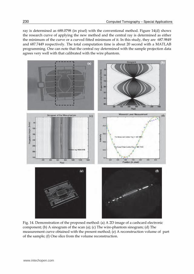
2.2.2 Experimental demonstration and discussion To evaluate the accuracy of the proposed method, an experiment was arranged to scan an electronic component used in a cashcard and a wire phantom at the same position. Figure 14(a) is a 2D image of the sample and Figure 14(b) shows a central slice sinogram of the scan. The sinogram of the wire phantom is shown in Figure 14(c), from which the central

www.intechopen.com


230

ray is determined as 688.0798 (in pixel) with the conventional method. Figure 14(d) shows the research curve of applying the new method and the central ray is determined as either the minimum of the curve or a curved fitted minimum of it. In this study, they are 687.9849 and 687.7449 respectively. The total computation time is about 20 second with a MATLAB programming. One can note that the central ray determined with the sample projection data agrees very well with that calibrated with the wire phantom.

Fig. 14. Demonstration of the proposed method: (a) A 2D image of a cashcard electronic component; (b) A sinogram of the scan (a); (c) The wire-phantom sinogram; (d) The measurement curve obtained with the present method; (e) A reconstruction volume of part of the sample; (f) One slice from the volume reconstruction.

www.intechopen.com


231

With the central ray determined, the central part of object (the dash line-box area in Figure 14(a) was reconstructed using a volume cone-beam algorithm, written by the author in Matlab. Figures 14(e) and 14(f) show respectively the 3D result and one of the slices, from which one can see that the small wires are clearly reconstructed. This is an indication that the reconstruction is performed with an accurate central ray value.

(a) (b)

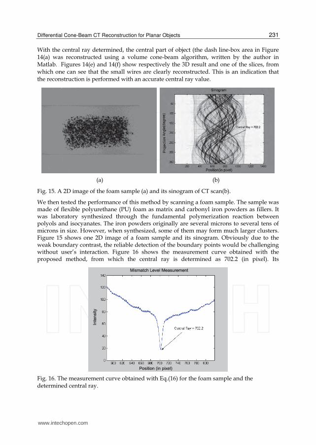
Fig. 15. A 2D image of the foam sample (a) and its sinogram of CT scan(b).

We then tested the performance of this method by scanning a foam sample. The sample was made of flexible polyurethane (PU) foam as matrix and carbonyl iron powders as fillers. It was laboratory synthesized through the fundamental polymerization reaction between polyols and isocyanates. The iron powders originally are several microns to several tens of microns in size. However, when synthesized, some of them may form much larger clusters. Figure 15 shows one 2D image of a foam sample and its sinogram. Obviously due to the weak boundary contrast, the reliable detection of the boundary points would be challenging without user’s interaction. Figure 16 shows the measurement curve obtained with the proposed method, from which the central ray is determined as 702.2 (in pixel). Its

Fig. 16. The measurement curve obtained with Eq.(16) for the foam sample and the determined central ray.

www.intechopen.com


232

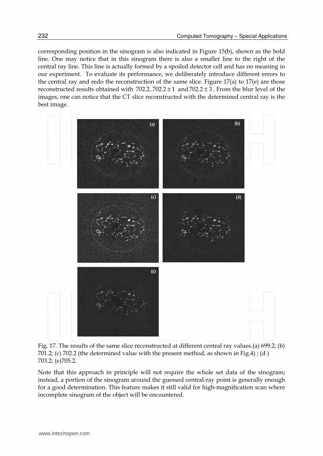
corresponding position in the sinogram is also indicated in Figure 15(b), shown as the bold line. One may notice that in this sinogram there is also a smaller line to the right of the central ray line. This line is actually formed by a spoiled detector cell and has no meaning in our experiment. To evaluate its performance, we deliberately introduce different errors to the central ray and redo the reconstruction of the same slice. Figure 17(a) to 17(e) are those reconstructed results obtained with 702.2, 702.2 1± and 702.2 3± . From the blur level of the images, one can notice that the CT slice reconstructed with the determined central ray is the best image.

Fig. 17. The results of the same slice reconstructed at different central ray values.(a) 699.2; (b) 701.2; (c) 702.2 (the determined value with the present method, as shown in Fig.4) ; (d ) 703.2; (e)705.2.

Note that this approach in principle will not require the whole set data of the sinogram; instead, a portion of the sinogram around the guessed central-ray point is generally enough for a good determination. This feature makes it still valid for high-magnification scan where incomplete sinogram of the object will be encountered.

www.intechopen.com


233

3. Cone-beam CT reconstruction for planar objects

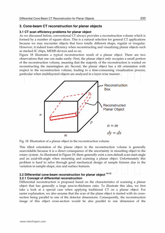
3.1 CT scan efficiency problems for planar object As we discussed before, conventional CT always provides a reconstruction volume which is formed by a number of square slices. This is a natural selection for general CT applications because we may encounter objects that have totally different shape, regular or irregular. However, it indeed loses efficiency when reconstructing and visualizing planar objects such as stacked IC chips, MEMS devices and so on. Figure 18 illustrates a typical reconstruction result of a planar object. There are two observations that one can make easily: First, the planar object only occupies a small portion of the reconstruction volume, meaning that the majority of the reconstruction is wasted on reconstructing the meaningless air; Second, the planar object has a tilt orientation with respect to the reconstruction volume, leading to a time-consuming visualization process, particular when multilayered objects are analyzed in a layer-wise manner.

Fig. 18. Illustration of a planar object in the reconstruction volume

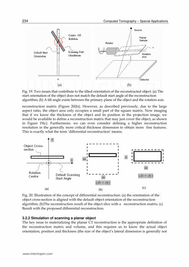
This tilted orientation of the planar object in the reconstruction volume is generally unavoidable because it is a direct consequence of the uncertainty in mounting object to the rotary system. As illustrated in Figure 19, there generally exist a non-default scan-start-angle and an axial-tilt-angle when mounting and scanning a planar object. Unfortunately this problem is hard to solve through good mechanical design of sample fixtures due to the variation in sample shape, size and surface features.

3.2 Differential cone-beam reconstruction for planar object 14-15

3.2.1 Concept of differential reconstruction Differential reconstruction is proposed based on the characteristics of scanning a planar object that has generally a large area-to-thickness ratio. To illustrate this idea, we first take a look at a special case when applying traditional CT on a planar object. For easier explanation, we also assume that the scan of the plane object is started with its cross-section being parallel to one of the detector dimensions. Consequently, the reconstruction image of this object cross-section would be also parallel to one dimension of the

www.intechopen.com


234

(a) (b)

Fig. 19. Two issues that contribute to the tilted orientation of the reconstructed object: (a) The start orientation of the object does not match the default start angle of the reconstruction algorithm; (b) A tilt angle exists between the primary plane of the object and the rotation axis.

reconstruction matrix (Figure 20(b)). However, as described previously, due to the large aspect ratio, the object area only occupies a small part of the square matrix. Now imaging that if we know the thickness of the object and its position in the projection image, we would be available to define a reconstruction matrix that may just cover the object, as shown in Figure 19(c). Furthermore, we can even consider defining a higher reconstruction resolution in the generally more critical thickness dimension to obtain more fine features. This is exactly what the term ‘differential reconstruction’ means.

Fig. 20. Illustration of the concept of differential reconstruction: (a) the orientation of the object cross-section is aligned with the default object orientation of the reconstruction algorithm; (b)The reconstruction result of the object slice with a reconstruction matrix; (c) Result with the proposed differential reconstruction.

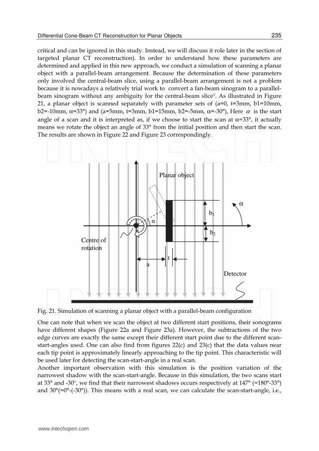
3.2.2 Simulation of scanning a planar object The key issue to materializing the planar CT reconstruction is the appropriate definition of

the reconstruction matrix and volume, and this requires us to know the actual object

orientation, position and thickness (the size of the object’s lateral dimension is generally not

www.intechopen.com


235

critical and can be ignored in this study. Instead, we will discuss it role later in the section of

targeted planar CT reconstruction). In order to understand how these parameters are

determined and applied in this new approach, we conduct a simulation of scanning a planar

object with a parallel-beam arrangement. Because the determination of these parameters

only involved the central-beam slice, using a parallel-beam arrangement is not a problem

because it is nowadays a relatively trial work to convert a fan-beam sinogram to a parallel-

beam sinogram without any ambiguity for the central-beam slice7. As illustrated in Figure

21, a planar object is scanned separately with parameter sets of (a=0, t=3mm, b1=10mm,

b2=-10mm, α=33°) and (a=5mm, t=3mm, b1=15mm, b2=-5mm, α=-30°), Here α is the start

angle of a scan and it is interpreted as, if we choose to start the scan at α=33°, it actually

means we rotate the object an angle of 33° from the initial position and then start the scan.

The results are shown in Figure 22 and Figure 23 correspondingly.

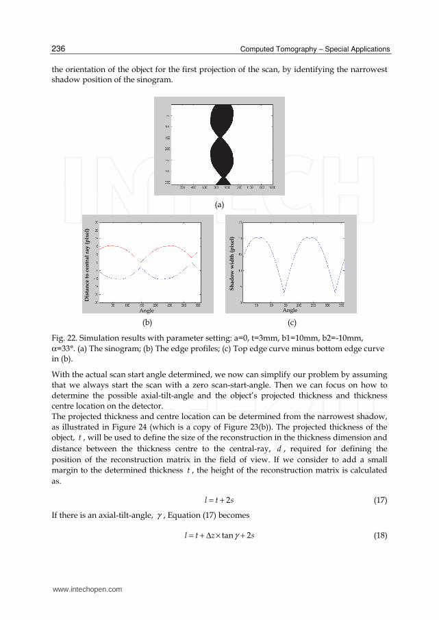
Fig. 21. Simulation of scanning a planar object with a parallel-beam configuration

One can note that when we scan the object at two different start positions, their sonograms

have different shapes (Figure 22a and Figure 23a). However, the subtractions of the two

edge curves are exactly the same except their different start point due to the different scan-

start-angles used. One can also find from figures 22(c) and 23(c) that the data values near

each tip point is approximately linearly approaching to the tip point. This characteristic will

be used later for detecting the scan-start-angle in a real scan.

Another important observation with this simulation is the position variation of the narrowest shadow with the scan-start-angle. Because in this simulation, the two scans start

at 33° and -30°, we find that their narrowest shadows occurs respectively at 147° (=180°-33°) and 30°(=0°-(-30°)). This means with a real scan, we can calculate the scan-start-angle, i.e.,

Centre of

rotation

a t

b2

b1

Planar object

Detector

α

α

www.intechopen.com


236

the orientation of the object for the first projection of the scan, by identifying the narrowest shadow position of the sinogram.

(a)

(b) (c)

Fig. 22. Simulation results with parameter setting: a=0, t=3mm, b1=10mm, b2=-10mm,

α=33°. (a) The sinogram; (b) The edge profiles; (c) Top edge curve minus bottom edge curve in (b).

With the actual scan start angle determined, we now can simplify our problem by assuming

that we always start the scan with a zero scan-start-angle. Then we can focus on how to

determine the possible axial-tilt-angle and the object’s projected thickness and thickness

centre location on the detector.

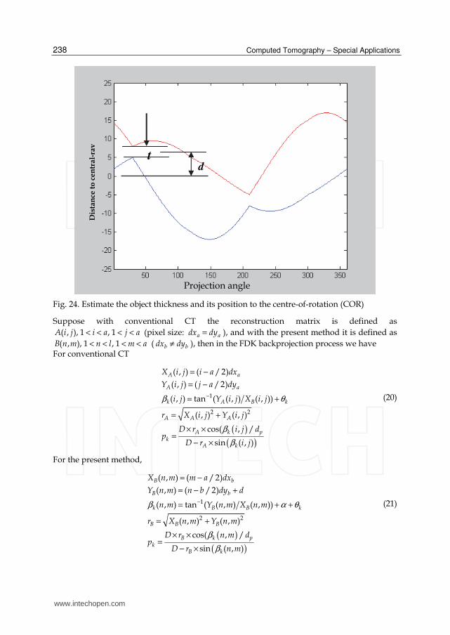
The projected thickness and centre location can be determined from the narrowest shadow,

as illustrated in Figure 24 (which is a copy of Figure 23(b)). The projected thickness of the

object, t , will be used to define the size of the reconstruction in the thickness dimension and

distance between the thickness centre to the central-ray, d , required for defining the

position of the reconstruction matrix in the field of view. If we consider to add a small

margin to the determined thickness t , the height of the reconstruction matrix is calculated

as.

2l t s= + (17)

If there is an axial-tilt-angle, γ , Equation (17) becomes

tan 2l t z sγ= + Δ × + (18)

Angle Angle

Dis

tan

ce t

o c

en

tra

l ra

y (

pix

el)

Sh

ad

ow

wid

th (

pix

el)

www.intechopen.com


237

(a)

(b) (c)

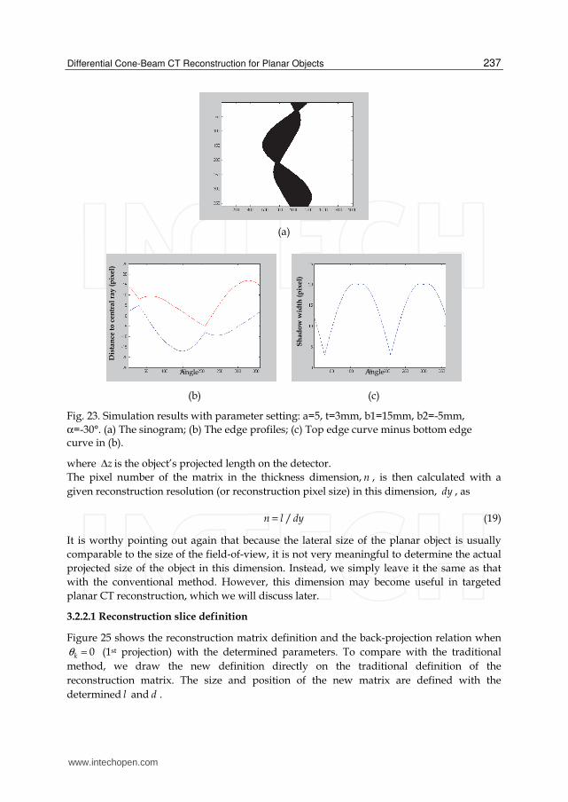
Fig. 23. Simulation results with parameter setting: a=5, t=3mm, b1=15mm, b2=-5mm,

α=-30°. (a) The sinogram; (b) The edge profiles; (c) Top edge curve minus bottom edge curve in (b).

where zΔ is the object’s projected length on the detector.

The pixel number of the matrix in the thickness dimension, n , is then calculated with a

given reconstruction resolution (or reconstruction pixel size) in this dimension, dy , as

/n l dy= (19)

It is worthy pointing out again that because the lateral size of the planar object is usually

comparable to the size of the field-of-view, it is not very meaningful to determine the actual

projected size of the object in this dimension. Instead, we simply leave it the same as that

with the conventional method. However, this dimension may become useful in targeted

planar CT reconstruction, which we will discuss later.

3.2.2.1 Reconstruction slice definition

Figure 25 shows the reconstruction matrix definition and the back-projection relation when

0kθ = (1st projection) with the determined parameters. To compare with the traditional

method, we draw the new definition directly on the traditional definition of the

reconstruction matrix. The size and position of the new matrix are defined with the

determined l and d .

Angle Angle

Dis

tan

ce t

o c

en

tra

l ra

y (

pix

el)

Sh

ad

ow

wid

th (

pix

el)

www.intechopen.com


238

Fig. 24. Estimate the object thickness and its position to the centre-of-rotation (COR)

Suppose with conventional CT the reconstruction matrix is defined as

( , ), 1 , 1A i j i a j a< < < < (pixel size: a adx dy= ), and with the present method it is defined as

( , ), 1 , 1B n m n l m a< < < < ( b bdx dy≠ ), then in the FDK backprojection process we have For conventional CT

( )( )

1

2 2

( , ) ( / 2)

( , ) ( / 2)

( , ) tan ( ( , ) ( , ))

( , ) ( , )

cos( , /

sin ( , )

A a

A a

k A B k

A A A

A k pk

A k

X i j i a dx

Y i j j a dy

i j Y i j X i j

r X i j Y i j

D r i j dp

D r i j

β θ

β

β

−

= −

= −

= +

= +

× ×=

− ×

(20)

For the present method,

( )

( )

1

2 2

( , ) ( / 2)

( , ) ( / 2)

( , ) tan ( ( , ) ( , ))

( , ) ( , )

cos( , /

sin ( , )

B b

B b

k B B k

B B B

B k pk

B k

X n m m a dx

Y n m n b dy d

n m Y n m X n m

r X n m Y n m

D r n m dp

D r n m

β α θ

β

β

−

= −

= − +

= + +

= +

× ×=

− ×

(21)

t d

Dis

tan

ce t

o c

en

tra

l-ra

y

Projection angle

www.intechopen.com


239

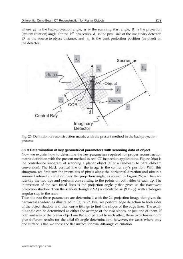
where kβ is the back-projection angle, α is the scanning start angle, kθ is the projection

(system rotation) angle for the thk projection, pd is the pixel size of the imaginary detector,

D is the source-to-object distance, and kp is the back-projection position (in pixel) on

the detector.

Fig. 25. Definition of reconstruction matrix with the present method in the backprojection process

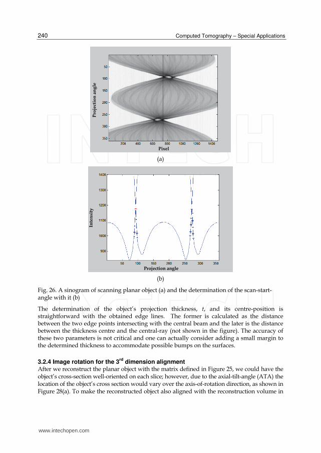
3.2.3 Determination of key geometrical parameters with scanning data of object

Now we explain how to determine the key parameters required for proper reconstruction

matrix definition with the present method in real CT inspection applications. Figure 26(a) is

the central-slice sinogram of scanning a planar object (after a fan-beam to parallel-beam

conversion). The black vertical line on the image is the central ray’s position. With this

sinogram, we first sum the intensities of pixels along the horizontal direction and obtain a

summed intensity variation over the projection angle, as shown in Figure 26(b). Then we

identify the two tips and perform curve fitting to the points on both sides of each tip. The

intersection of the two fitted lines is the projection angle γ that gives us the narrowest

projection shadow. Then the scan-start-angle (SSA) is calculated as (90 )γ° − with a 1-degree

angular step in the scan. Then the rest three parameters are determined with the 2d projection image that gives the

narrowest shadow, as illustrated in figure 27. First we perform edge detection to both sides

of the object shadow and then curve fittings to find the slopes of the edge lines. The axial-

tilt-angle can be determined as either the average of the two slopes, or just one of them. If

both surfaces of the planar object are flat and parallel to each other, these two choices don’t

give different results for the axial-tilt-angle determination; however, for cases where only

one surface is flat, we chose the flat surface for axial-tilt-angle calculation.

www.intechopen.com


240

(a)

(b)

Fig. 26. A sinogram of scanning planar object (a) and the determination of the scan-start-angle with it (b)

The determination of the object’s projection thickness, t, and its centre-position is straightforward with the obtained edge lines. The former is calculated as the distance between the two edge points intersecting with the central beam and the later is the distance between the thickness centre and the central-ray (not shown in the figure). The accuracy of these two parameters is not critical and one can actually consider adding a small margin to the determined thickness to accommodate possible bumps on the surfaces.

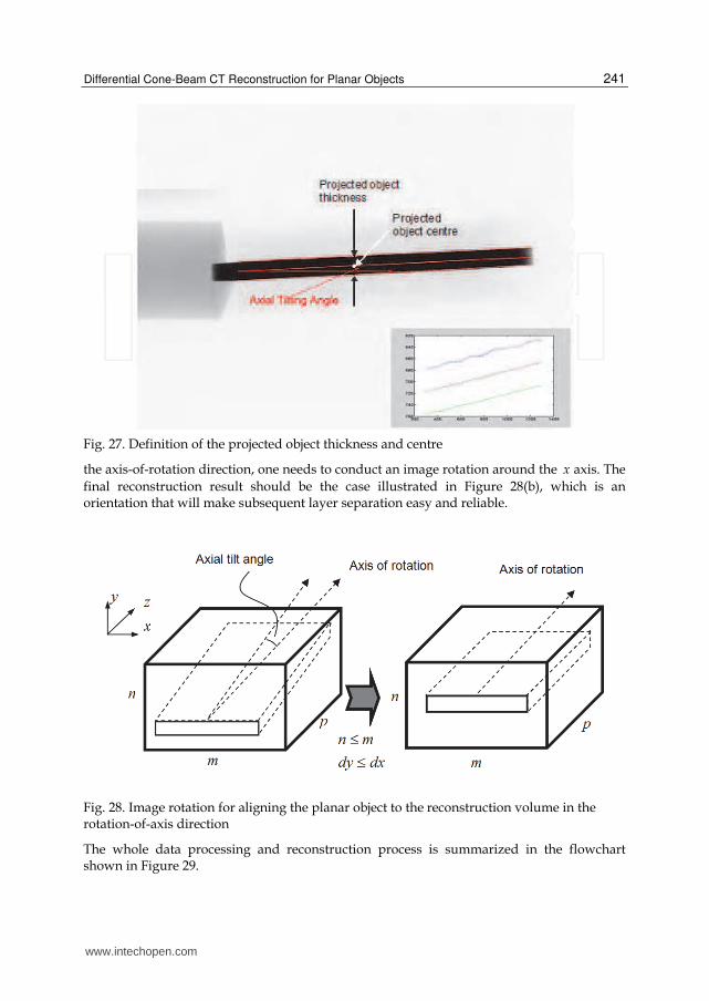
3.2.4 Image rotation for the 3rd

dimension alignment After we reconstruct the planar object with the matrix defined in Figure 25, we could have the object’s cross-section well-oriented on each slice; however, due to the axial-tilt-angle (ATA) the location of the object’s cross section would vary over the axis-of-rotation direction, as shown in Figure 28(a). To make the reconstructed object also aligned with the reconstruction volume in

Pixel

Projection angle

Pro

ject

ion

an

gle

In

ten

sity

www.intechopen.com


241

Fig. 27. Definition of the projected object thickness and centre

the axis-of-rotation direction, one needs to conduct an image rotation around the x axis. The

final reconstruction result should be the case illustrated in Figure 28(b), which is an orientation that will make subsequent layer separation easy and reliable.

Fig. 28. Image rotation for aligning the planar object to the reconstruction volume in the rotation-of-axis direction

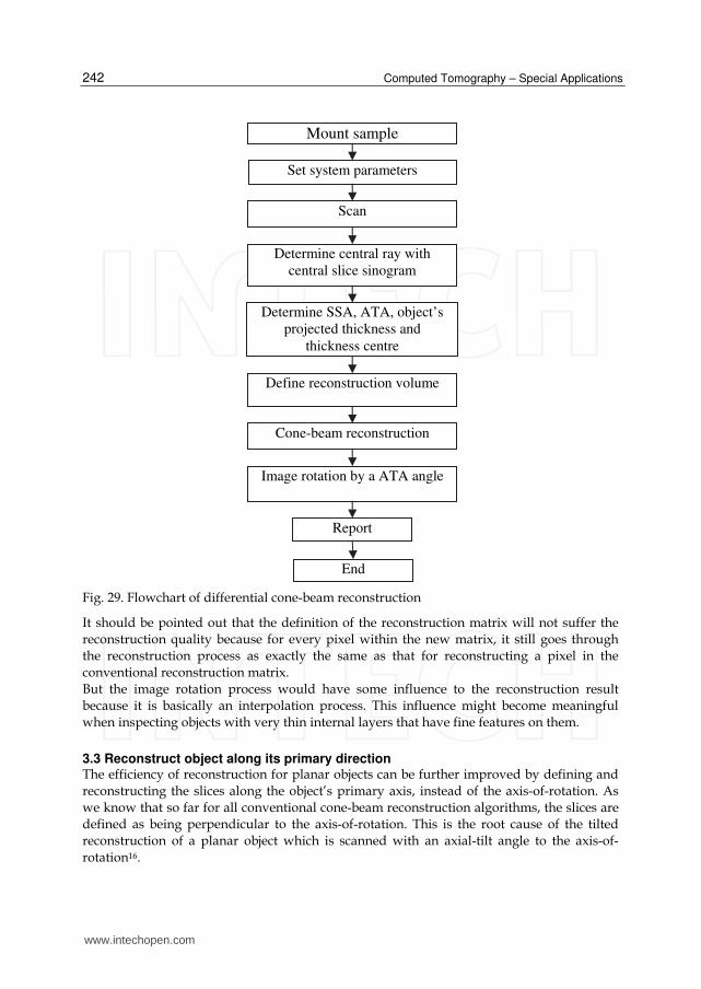
The whole data processing and reconstruction process is summarized in the flowchart shown in Figure 29.

www.intechopen.com


242

Fig. 29. Flowchart of differential cone-beam reconstruction

It should be pointed out that the definition of the reconstruction matrix will not suffer the

reconstruction quality because for every pixel within the new matrix, it still goes through

the reconstruction process as exactly the same as that for reconstructing a pixel in the

conventional reconstruction matrix.

But the image rotation process would have some influence to the reconstruction result

because it is basically an interpolation process. This influence might become meaningful

when inspecting objects with very thin internal layers that have fine features on them.

3.3 Reconstruct object along its primary direction The efficiency of reconstruction for planar objects can be further improved by defining and

reconstructing the slices along the object’s primary axis, instead of the axis-of-rotation. As

we know that so far for all conventional cone-beam reconstruction algorithms, the slices are

defined as being perpendicular to the axis-of-rotation. This is the root cause of the tilted

reconstruction of a planar object which is scanned with an axial-tilt angle to the axis-of-

rotation16.

Mount sample

Set system parameters

Scan

Determine central ray with

central slice sinogram

Define reconstruction volume

Determine SSA, ATA, object’s

projected thickness and

thickness centre

Cone-beam reconstruction

Image rotation by a ATA angle

Report

End

www.intechopen.com


243

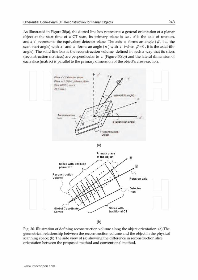
As illustrated in Figure 30(a), the dotted-line box represents a general orientation of a planar

object at the start time of a CT scan, its primary plane is xz . 'z is the axis of rotation,

and ' 'x z represents the equivalent detector plane. The axis x forms an angle ( β , i.e., the

scan-start-angle) with 'x and z forms an angle (α ) with 'z (when 0β = , it is the axial-tilt-

angle). The solid-line box is the reconstruction volume, defined in such a way that its slices

(reconstruction matrices) are perpendicular to z (Figure 30(b)) and the lateral dimension of

each slice (matrix) is parallel to the primary dimension of the object’s cross-section.

(a)

(b)

Fig. 30. Illustration of defining reconstruction volume along the object orientation. (a) The geometrical relationship between the reconstruction volume and the object in the physical scanning space; (b) The side view of (a) showing the difference in reconstruction slice orientation between the proposed method and conventional method.

www.intechopen.com


244

Although the concept of the present idea looks quite straightforward and simple, its implementation is definitely not so. Fortunately, it is possible for us to decouple the roles of the scan-start-angle and the axial-tilt angle in the reconstruction process. Considering the fact that we can always rearrange the projections to an equivalent scan that starts with a zero scan-start angle by assigning the actual scan-stat-angle to the first projection, we just need to consider a non-zero axial-tilt-angle situation in developing the reconstruction algorithm for the proposed method.

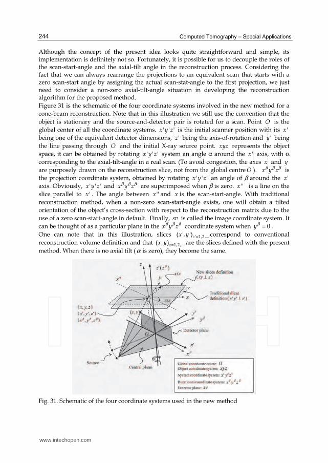
Figure 31 is the schematic of the four coordinate systems involved in the new method for a

cone-beam reconstruction. Note that in this illustration we still use the convention that the

object is stationary and the source-and-detector pair is rotated for a scan. Point O is the

global center of all the coordinate systems. ' ' 'x y z is the initial scanner position with its 'x

being one of the equivalent detector dimensions, 'z being the axis-of-rotation and 'y being

the line passing through O and the initial X-ray source point. xyz represents the object

space, it can be obtained by rotating ' ' 'x y z system an angle α around the 'x axis, with α

corresponding to the axial-tilt-angle in a real scan. (To avoid congestion, the axes x and y

are purposely drawn on the reconstruction slice, not from the global centre O ). x y zβ β β is

the projection coordinate system, obtained by rotating ' ' 'x y z an angle of β around the 'z

axis. Obviously, ' ' 'x y z and x y zβ β β are superimposed when β is zero. ''x is a line on the

slice parallel to 'x . The angle between ''x and x is the scan-start-angle. With traditional

reconstruction method, when a non-zero scan-start-angle exists, one will obtain a tilted

orientation of the object’s cross-section with respect to the reconstruction matrix due to the

use of a zero scan-start-angle in default. Finally, sv is called the image coordinate system. It

can be thought of as a particular plane in the x y zβ β β coordinate system when 0yβ = .

One can note that in this illustration, slices ' 1,2 ,...( ', ')zx y = correspond to conventional

reconstruction volume definition and that 1,2,...( , )zx y = are the slices defined with the present

method. When there is no axial tilt (α is zero), they become the same.

Fig. 31. Schematic of the four coordinate systems used in the new method

www.intechopen.com


245

Similar to deriving the conventional algorithm7, the key job here is to establish the

relationship between an object point ( , ,x y z ) and its projection position ( ,s vβ β ) at each

projection angle β . With the proposed method, ( ,s v ) is calculated as

cos sin ( cos sin )

sin cos( sin cos ( cos sin ))

s x y zD

y zD x y zv

β

β

β β α α

α αβ β α α

− + = − +− + + (22a)

And the object function can be reconstructed as:

( ) ( )

2 2 '

2 22

1( , , ) ( ) ( , , ) ( )

2 '( )

m

m

D Df x y z d q s v h s s ds

D yD s v

π γ γ β β β β

γ γβ β

β β−

− −= −

++ +

(22b)

3.4 Targeted CT reconstruction for planar object17

Targeted reconstruction is adopted in CT inspection practice to achieve high-resolution reconstruction to a small region-of-interest(ROI). This is particularly useful when scanning a large IC chip on which only a small region is interesting to us. Instead of reconstructing the whole IC chip in the field of-view, only the ROI is reconstructed. In conventional targeted reconstruction, the common practice is to do a normal reconstruction first, from which the ROI is identified and re-reconstructed. Now we discuss how to extend the developed algorithm to targeted reconstruction of planar ROI on a planar object. But unlike conventional targeted reconstruction, the present method only needs one reconstruction process. Besides, it still possesses all advantages of the planar CT reconstruction technology such as the well-orientated reconstruction, flexible reconstruction resolution definition and easy visualization.

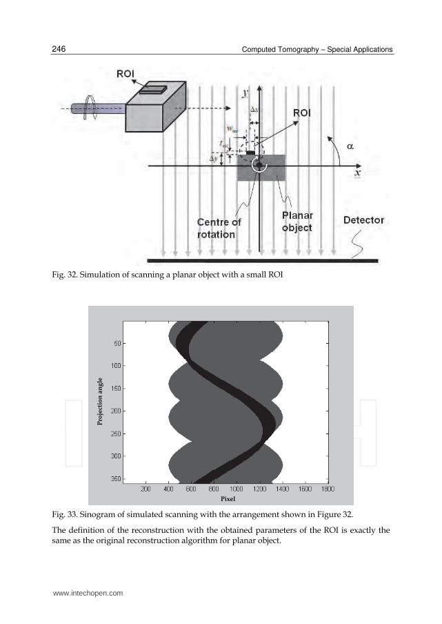
3.4.1 Simulation of scanning a planar object with a small planar ROI

To describe the concept of the proposed targeted reconstruction, as before, we first conduct

a simulation to examine the projection property of the different parts of the components. As

shown in Figure 32, a planar ROI (cross-sectional size: roi roiw t× ) is on top of a planar

substrate with distances xΔ and yΔ to the centre-of-rotation respectively in x and y . By

scanning this structure with a parallel-beam arrangement, we obtain a sinogram shown in

Figure 33. Because only the shadow boundary information of the two parts is useful to us in

determining the required parameters that are discussed later, the gradual variation in

attenuation during the rotation is not considered in the simulation. Instead, we simply

assume that the substrate and the ROI generate two different but constant shadow gray-

levels during the scan.

Figure 34 shows the boundary curves of the two parts extracted from the sinogram in Figure

33, in which the dotted lines represent the projections of the substrate and the solid lines

represent the ROI. As with the original method, the scan start angle can be determined by

identifying the projection index that gives the narrowest shadow of the substrate on the

detector (points A and B). Then the projected thickness ( roit ) of the ROI and its centre can be

determined by identifying the two edge points of the ROI at this position.

Then we consider the determination of the other two parameters, i.e., roiw and xΔ in Figure

32, which are measured as the width and centre of the ROI shadow at a position 270 degree

away for the narrowest position identified, as illustrated in Figure 34.

www.intechopen.com


246

Fig. 32. Simulation of scanning a planar object with a small ROI

Fig. 33. Sinogram of simulated scanning with the arrangement shown in Figure 32.

The definition of the reconstruction with the obtained parameters of the ROI is exactly the same as the original reconstruction algorithm for planar object.

Pixel

Pro

ject

ion

an

gle

www.intechopen.com


247

Fig. 34. The edge profiles of the two parts of the components

3.4.2 Implementation of the targeted reconstruction

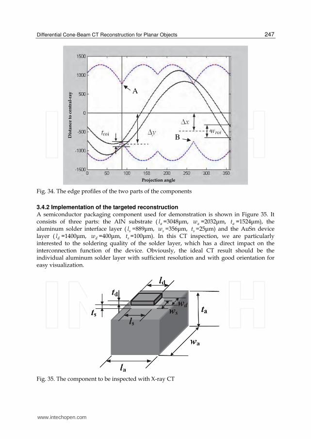
A semiconductor packaging component used for demonstration is shown in Figure 35. It consists of three parts: the AIN substrate ( al =3048μm, aw =2032μm, at =1524μm), the aluminum solder interface layer ( sl =889μm, sw =356μm, st =25μm) and the AuSn device layer ( dl =1400μm, dw =400μm, st =100μm). In this CT inspection, we are particularly interested to the soldering quality of the solder layer, which has a direct impact on the interconnection function of the device. Obviously, the ideal CT result should be the individual aluminum solder layer with sufficient resolution and with good orientation for easy visualization.

Fig. 35. The component to be inspected with X-ray CT

B

A

Projection angle

Dis

tan

ce t

o c

en

tra

l-ra

y

www.intechopen.com


248

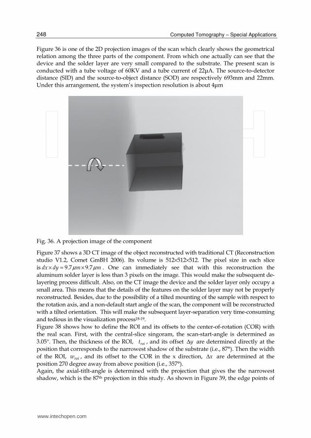
Figure 36 is one of the 2D projection images of the scan which clearly shows the geometrical relation among the three parts of the component. From which one actually can see that the device and the solder layer are very small compared to the substrate. The present scan is conducted with a tube voltage of 60KV and a tube current of 22μA. The source-to-detector distance (SID) and the source-to-object distance (SOD) are respectively 693mm and 22mm. Under this arrangement, the system’s inspection resolution is about 4μm

Fig. 36. A projection image of the component

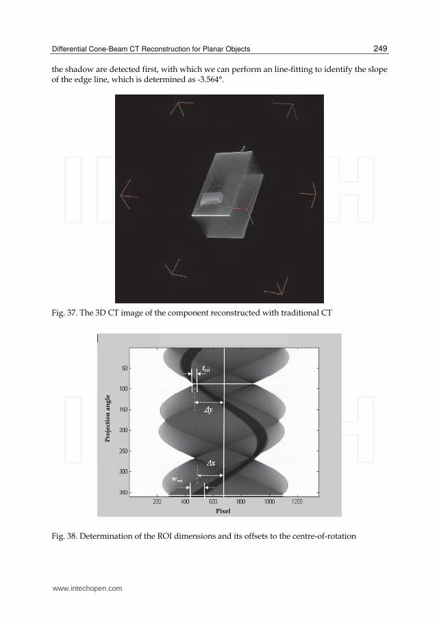
Figure 37 shows a 3D CT image of the object reconstructed with traditional CT (Reconstruction

studio V1.2, Comet GmBH 2006). Its volume is 512×512×512. The pixel size in each slice

is 9.7 9.7dx dy m mµ µ× = × . One can immediately see that with this reconstruction the

aluminum solder layer is less than 3 pixels on the image. This would make the subsequent de-

layering process difficult. Also, on the CT image the device and the solder layer only occupy a

small area. This means that the details of the features on the solder layer may not be properly

reconstructed. Besides, due to the possibility of a tilted mounting of the sample with respect to

the rotation axis, and a non-default start angle of the scan, the component will be reconstructed

with a tilted orientation. This will make the subsequent layer-separation very time-consuming

and tedious in the visualization process18-19.

Figure 38 shows how to define the ROI and its offsets to the center-of-rotation (COR) with

the real scan. First, with the central-slice singoram, the scan-start-angle is determined as

3.05°. Then, the thickness of the ROI, roit , and its offset yΔ are determined directly at the

position that corresponds to the narrowest shadow of the substrate (i.e., 87°). Then the width

of the ROI, roiw , and its offset to the COR in the x direction, xΔ are determined at the

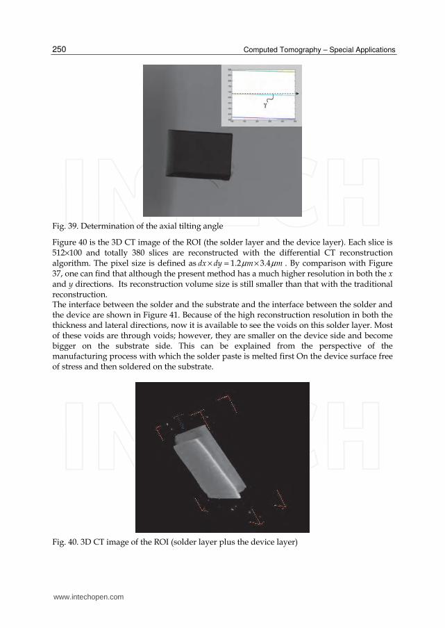
position 270 degree away from above position (i.e., 357°). Again, the axial-titlt-angle is determined with the projection that gives the the narrowest shadow, which is the 87th projection in this study. As shown in Figure 39, the edge points of

www.intechopen.com


249

the shadow are detected first, with which we can perform an line-fitting to identify the slope of the edge line, which is determined as -3.564°.

Fig. 37. The 3D CT image of the component reconstructed with traditional CT

Fig. 38. Determination of the ROI dimensions and its offsets to the centre-of-rotation

Pixel

Pro

ject

ion

an

gle

www.intechopen.com


250

Fig. 39. Determination of the axial tilting angle

Figure 40 is the 3D CT image of the ROI (the solder layer and the device layer). Each slice is 512×100 and totally 380 slices are reconstructed with the differential CT reconstruction algorithm. The pixel size is defined as 1.2 3.4dx dy m mµ µ× = × . By comparison with Figure 37, one can find that although the present method has a much higher resolution in both the x and y directions. Its reconstruction volume size is still smaller than that with the traditional reconstruction. The interface between the solder and the substrate and the interface between the solder and the device are shown in Figure 41. Because of the high reconstruction resolution in both the thickness and lateral directions, now it is available to see the voids on this solder layer. Most of these voids are through voids; however, they are smaller on the device side and become bigger on the substrate side. This can be explained from the perspective of the manufacturing process with which the solder paste is melted first On the device surface free of stress and then soldered on the substrate.

Fig. 40. 3D CT image of the ROI (solder layer plus the device layer)

www.intechopen.com


251

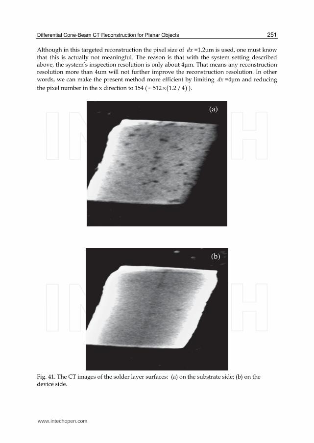
Although in this targeted reconstruction the pixel size of dx =1.2μm is used, one must know

that this is actually not meaningful. The reason is that with the system setting described above, the system’s inspection resolution is only about 4μm. That means any reconstruction resolution more than 4um will not further improve the reconstruction resolution. In other

words, we can make the present method more efficient by limiting dx =4μm and reducing

the pixel number in the x direction to 154 ( ( )512 1.2 / 4≈ × ).

Fig. 41. The CT images of the solder layer surfaces: (a) on the substrate side; (b) on the device side.

(a)

(b)

www.intechopen.com


252

3.5 CT inspection of a region-of-interest on a curved planar structure20

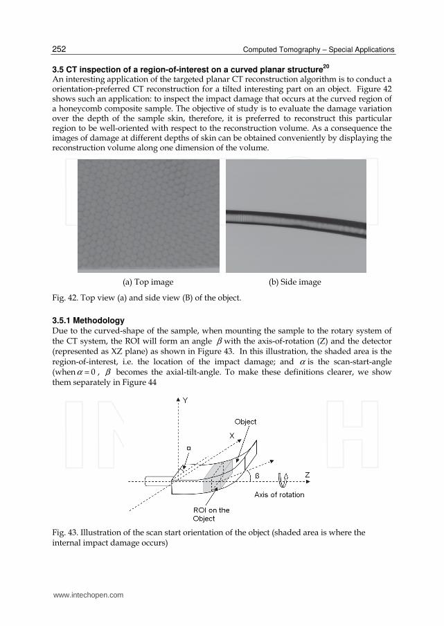
An interesting application of the targeted planar CT reconstruction algorithm is to conduct a orientation-preferred CT reconstruction for a tilted interesting part on an object. Figure 42 shows such an application: to inspect the impact damage that occurs at the curved region of a honeycomb composite sample. The objective of study is to evaluate the damage variation over the depth of the sample skin, therefore, it is preferred to reconstruct this particular region to be well-oriented with respect to the reconstruction volume. As a consequence the images of damage at different depths of skin can be obtained conveniently by displaying the reconstruction volume along one dimension of the volume.

(a) Top image (b) Side image

Fig. 42. Top view (a) and side view (B) of the object.

3.5.1 Methodology

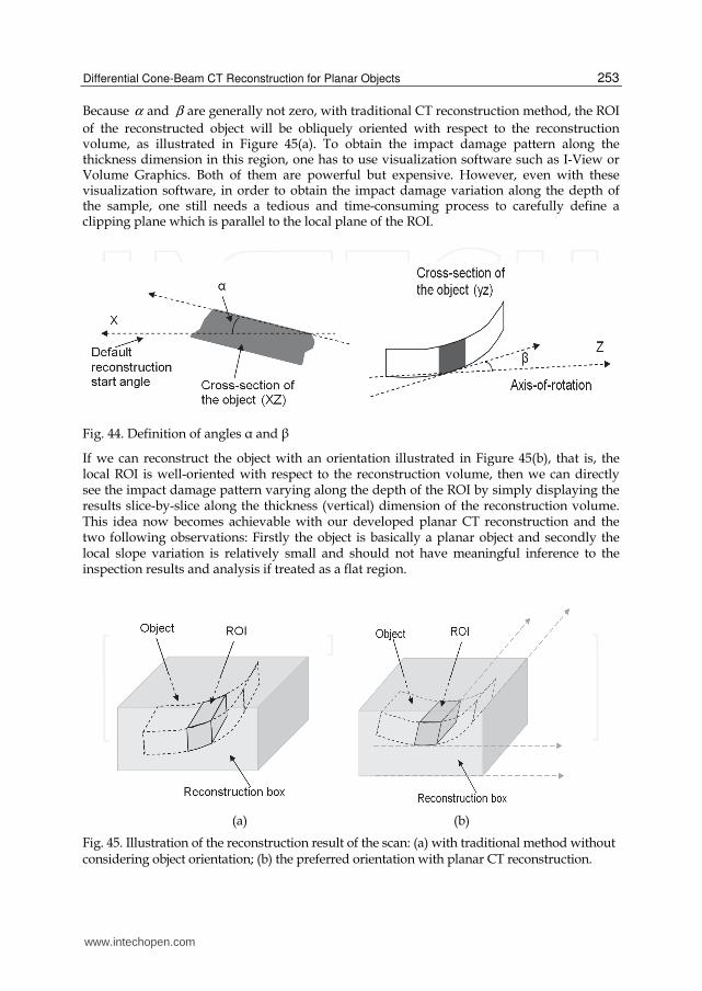
Due to the curved-shape of the sample, when mounting the sample to the rotary system of the CT system, the ROI will form an angle β with the axis-of-rotation (Z) and the detector (represented as XZ plane) as shown in Figure 43. In this illustration, the shaded area is the region-of-interest, i.e. the location of the impact damage; and α is the scan-start-angle (when 0α = , β becomes the axial-tilt-angle. To make these definitions clearer, we show them separately in Figure 44

Fig. 43. Illustration of the scan start orientation of the object (shaded area is where the internal impact damage occurs)

www.intechopen.com


253

Because α and β are generally not zero, with traditional CT reconstruction method, the ROI

of the reconstructed object will be obliquely oriented with respect to the reconstruction volume, as illustrated in Figure 45(a). To obtain the impact damage pattern along the thickness dimension in this region, one has to use visualization software such as I-View or Volume Graphics. Both of them are powerful but expensive. However, even with these visualization software, in order to obtain the impact damage variation along the depth of the sample, one still needs a tedious and time-consuming process to carefully define a clipping plane which is parallel to the local plane of the ROI.

Fig. 44. Definition of angles ┙ and ┚

If we can reconstruct the object with an orientation illustrated in Figure 45(b), that is, the local ROI is well-oriented with respect to the reconstruction volume, then we can directly see the impact damage pattern varying along the depth of the ROI by simply displaying the results slice-by-slice along the thickness (vertical) dimension of the reconstruction volume. This idea now becomes achievable with our developed planar CT reconstruction and the two following observations: Firstly the object is basically a planar object and secondly the local slope variation is relatively small and should not have meaningful inference to the inspection results and analysis if treated as a flat region.

(a) (b)

Fig. 45. Illustration of the reconstruction result of the scan: (a) with traditional method without considering object orientation; (b) the preferred orientation with planar CT reconstruction.

www.intechopen.com


254

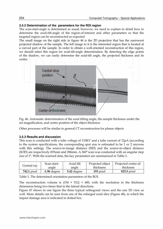
3.5.2 Determination of the parameters for the ROI region The scan-start-angle is determined as usual, however, we need to explain in detail how to determine the axial-tilt-angle of the region-of-interest and other parameters so that the targeted region can be reconstructed as expected The small image on the right side in figure 46 is the 2D projection that has the narrowest projected shadow of the sample. The left image to it is the interested region that is located at a curved part of the sample. In order to obtain a well-oriented reconstruction of this region, we should select this region for axial-tilt-angle determination. By detecting the edge points of the shadow, we can easily determine the axial-tilt angle, the projected thickness and its centre.

Fig. 46. Automatic determination of the axial tilting angle, the sample thickness under the set magnification, and centre position of the object thickness

Other processes will be similar to general CT reconstruction for planar objects

3.5.3 Results and discussion This scan is conducted with a tube voltage of 110KV and a tube current of 12μA (according

to the system specifications, the corresponding spot size is estimated to be 1 or 2 microns with this setting). The source-to-image distance (SID) and the source-to-object distance (SOD) are respectively 693mm and 286mm. A 360° scan was conducted with an angular step

size of 1°. With the scanned data, the key parameters are summarized in Table 1.

Central ray Scan-start-

angle Axial tilt

angle Projected object

thickness Projected centre-of-

thickness

742.1 pixel -1.96 degree 5.42 degree 193 pixel 823.5 pixel

Table 1. The determined orientation parameters of the ROI.

The reconstruction volume is (154 × 512) × 600, with the resolution in the thickness

dimension being two times that in the lateral directions.

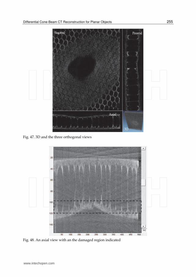
Figure 47 shows in one figure the three typical orthogonal views and the one 3D view as

well. More details can be seen from one of the enlarged axial slice (Figure 48), in which the

impact damage area is indicated in dotted box.

www.intechopen.com


255

Fig. 47. 3D and the three orthogonal views

Fig. 48. An axial view with an the damaged region indicated

www.intechopen.com


256

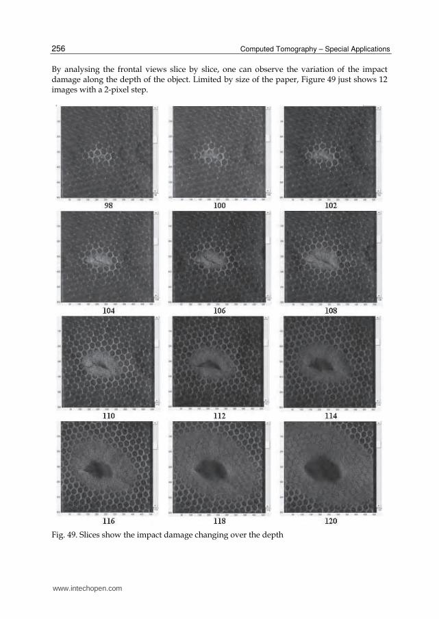
By analysing the frontal views slice by slice, one can observe the variation of the impact damage along the depth of the object. Limited by size of the paper, Figure 49 just shows 12 images with a 2-pixel step.

Fig. 49. Slices show the impact damage changing over the depth

www.intechopen.com


257

4. References

[1] Sun, Y.; Hou, Y.; Zhao, F. & Hu, J. (2006).A calibration method for misaligned scanner geometry in cone-beam computed tomography. NDT & E International Vol. 39, pp.499–513

[2] Shepp, L. A.; Hilal, S. K. & Schulz, R. A. (1979). The tuning fork artifact in computerized tomography. Computer Graphics Image Processiing. Vol. 10, pp.246-255.

[3] Taylor, T.& . Lupton, L. R. (1986). Resolution, artifacts and the design of computed tomography system. In: computed Tomography Systems, Sect. VIII. New York: Elsevier, pp.603-609

[4] Azevedo, S. G.; Schneberk, D. J.; Fitch, J. P. & Martz, H. E. (1990). Calculation of the rotational centers in computed tomography sinograms. IEEE Transaction on Nuclear Science. Vol. 37(4) pp.1525-1540

[5] Olander, B. (1994). Center of rotation determination using projection data in X-ray micro computed tomography. Report 77. Linköping University, Sweden, ISSN 1102-1799

[6] Ramachandran, G. N. & Lakshminarayanna, A. V. (1971). Three-dimensional reconstruction from radiographs and electron micrographs: Application of convolutions instead of Fourier transforms. Proceedings of the National Academy of Sciences of the USA, 68, p.2236

[7] Hsieh, J. (2003). Computed Tomography, SPIE PRESS, ISBN 0-8194-4425-1, Bellingham, Washington

[8] Kak, A. C. & Malcolm, S. (1999). Principle of Computerized Tomographic Imaging, IEEE Press, ISBN 0-87942-198-3, New York

[9] Banhart, J. (2008). Advanced Tomographic Methods in Materials Research and Engineering. Oxford University Press, ISBN 978-0-19-921324-5, New York

[10] Feinfocus Fox 160.25 Operation Instruction. (2004), Version 1.0 [11] Liu, T. & Malcolm, A. A. (2006). Micro-CT for minute objects with central ray

determined using the projection data of the objects. 9th European Conference on Non-Destructive Testing. (2006), (September 2006), Berlin, Germany

[12] Liu, T. & Malcolm, A.A. (2006). Comparison between four methods for central ray determination with wire phantom in micro-CT system. Optical Engineering, Vol. 45(6), 066402 1-5

[13] Liu, T. (2009). Direct Central Ray Determination in Micro-CT. Optical Engineering, vol. 48(NA), pp. 46501-46501

[14] Liu, T. (2009). Differential Reconstruction for Planar Object in Computed Tomography. Journal of X-ray Science and Technology.Vol. 17(2), pp.101-114

[15] Liu, T.; Wong, B. S. & Chai, T. C. (2008). A CT Reconstruction with Good-Orientation and Layer Separation for Multilayer Objects. 17th WCNDT, Shanghai, (October 2008)

[16] Liu, T (2011). Cone-beam reconstruction for planar objects. NDT & E International, under processing

[17] Liu, T.; Sim, L. M. & Xu, J. (2010). Targeted reconstruction with different planar computed tomography. NDT & E International Vol.43, pp.116-122

[18] User’s Manual, VGStudio Max 2.1, (2011) [19] Users Manual, i-View Workstation Version 1.0, ( 2003) [20] Liu, T.; Malcolm, A. A. & Xu, J. (2010). High-resolution X-ray CT inspection of

Honeycomb Composites Using Planar Computed Tomography Technology. 2nd

www.intechopen.com


258

International Symposium on DNT in Aerospace 2010 – We.4.B.4, (November 2010), Hamburg, Germany

[21] Kang, K.; Choi, M.; Kim, K.; Cha, Y.; Kang, Y.; Hong, D. & Yang, S. (2006). Inspection of impact damage in honeycomb composite plate by ESPI, Ultrasonic testing, and Thermography. 12th A-PCNDT– Asia-Pacific Conference on NDT, Auckland, New Zealand

[22] Abou-Khousa, M.A.; Ryley,A.; Kharkovsky, S.; Zoughi, R.; Daniels, D.; Kreitinger, N. & Steffes, G. (2007). Comparison of x-ray, millimeter wave, shearography and through-transmission ultrasonic methods for inspection of honeycomb composites. American Institute of Physics

www.intechopen.com

Computed Tomography - Special ApplicationsEdited by Dr. Luca Saba

ISBN 978-953-307-723-9Hard cover, 318 pagesPublisher InTechPublished online 21, November, 2011Published in print edition November, 2011

InTech EuropeUniversity Campus STeP Ri Slavka Krautzeka 83/A 51000 Rijeka, Croatia Phone: +385 (51) 770 447 Fax: +385 (51) 686 166www.intechopen.com

InTech ChinaUnit 405, Office Block, Hotel Equatorial Shanghai No.65, Yan An Road (West), Shanghai, 200040, China

Phone: +86-21-62489820 Fax: +86-21-62489821

CT has evolved into an indispensable imaging method in clinical routine. The first generation of CT scannersdeveloped in the 1970s and numerous innovations have improved the utility and application field of the CT,such as the introduction of helical systems that allowed the development of the "volumetric CT" concept.Recently interesting technical, anthropomorphic, forensic and archeological as well as paleontologicalapplications of computed tomography have been developed. These applications further strengthen the methodas a generic diagnostic tool for non destructive material testing and three dimensional visualization beyond itsmedical use.

How to referenceIn order to correctly reference this scholarly work, feel free to copy and paste the following:

Liu Tong (2011). Differential Cone-Beam CT Reconstruction for Planar Objects, Computed Tomography -Special Applications, Dr. Luca Saba (Ed.), ISBN: 978-953-307-723-9, InTech, Available from:http://www.intechopen.com/books/computed-tomography-special-applications/differential-cone-beam-ct-reconstruction-for-planar-objects

Documents

Differential Cone-Beam CT Reconstruction for Planar Objectscdn.intechopen.com/pdfs-wm/24027.pdf · Differential Cone-Beam CT Reconstruction for Planar Objects ... Differential Cone-Beam