AN OVERVIEW OF COMPUTATIONAL AEROACOUSTIC MODELINGAT NASA LANGLEY

DAVID P. LOCKARD

Aerodynamics, Aerothermodynamics, and Acoustics CompetencyNASA Langley Research Center

Hampton, VA 23681-2199, U.S.A

ABSTRACT

The use of computational techniques in the area of acoustics is known as computational aeroacoustics and hasshown great promise in recent years. Although an ultimate goal is to use computational simulations as a virtual windtunnel, the problem is so complex that blind applications of traditional algorithms are typically unable to produceacceptable results. The phenomena of interest are inherently unsteady and cover a wide range of frequencies andamplitudes. Nonetheless, with appropriate simplifications and special care to resolve specific phenomena, currentlyavailable methods can be used to solve important acoustic problems. These simulations can be used to complementexperiments, and often give much more detailed information than can be obtained in a wind tunnel. The use ofacoustic analogy methods to inexpensively determine far-field acoustics from near-field unsteadiness has greatlyreduced the computational requirements. A few examples of current applications of computational aeroacoustics atNASA Langley are given. There remains a large class of problems that require more accurate and efficient methods.Research to develop more advanced methods that are able to handle the geometric complexity of realistic problemsusing block-structured and unstructured grids are highlighted.

INTRODUCTION

Computational aeroacoustics is a very broad field that encompasses research that uses numerical simulations tobetter understand aerodynamic noise. There is a large computational effort at NASA Langley Research Center aimedat predicting and reducing aircraft noise, and this paper only attempts to give an overview of a representative fractionof that work. The problem is very difficult because the geometry and physics involved are often quite complex. It hastaken 30 years to achieve significant noise reduction for jet engines. Although great strides have been made in thereduction of jet noise through the use of high-bypass ratio engines, there is a lack of understanding of thefundamental noise sources in subsonic jets. Today, tonal noise from large inlet fans is also important. There is ageneral theory for fan noise, but calculations are still somewhat limited. Extensive research is ongoing in the areas ofduct and liner acoustics[1]. Furthermore, the engines are not the only noise source that must be considered.Reductions in jet noise have made the airframe a significant, and in some cases dominant source during landing. Theflaps, slats, and landing gear are all important contributors to the sound field. To achieve significant noise reduction,these three major landing systems and the engines must all be quieted commensurately.

The physics behind the unsteadiness that generates noise is also very complicated. Fluctuations tend to grow inshear layers and vortical structures. Resolving these features in a mean flow calculation can be difficult. Trying tocapture the unsteadiness growing in them is even more challenging. Separated regions, instabilities, and large andsmall scale turbulence structures can all contribute to the sound field. Furthermore, the energy that is radiated asnoise is typically only a small fraction of the total energy near the source. This is part of the scale disparity betweenacoustic and hydrodynamic fluctuations. The human ear is able to distinguish between signals with vastly varyingamplitudes, so it is typical to use a logarithmic scale to describe them. The sound pressure level (SPL) is given by

SPL = 20 log�p0rms

pref

�(1)

with units of decibels (dB). The reference pressurepref = 20� 10�6 Pa is the threshold of human hearing, andrmsmeans root mean square. The ratio of pressure amplitudes between a quiet conversation, 60 dB, and a rock concert,120 dB, is 1000. In addition, atmospheric pressure is 3500 times greater than the pressure amplitude of a 120 dBsignal. At 120 dB, one starts feeling discomfort and experiences a ringing in the ears. Although this level is very loud

1

to humans, it is so small that a typical computational fluid dynamics (CFD) simulation very easily loses the soundwaves among the large hydrodynamic fluctuations. Simultaneously resolving the hydrodynamic fluctuations and thewide range of acoustic signals is very difficult.

Acousticians also have to deal with very disparate length and time scales. Mostly people can hear fairly wellbetween frequencies of 100 Hz and 10 kHz. This corresponds to wavelengths of 0.11 ft (0.034 m) and 11 ft (3.4 m),respectively. Trying to have enough grid points in the domain to resolve the very short wavelength while having adomain large enough to encompass the long wavelength results in enormous grids. One is also faced with thechallenge of trying to propagate the signal to observers located at great distances from the sources. A similar scaleproblem occurs temporally. The wavelength� of an acoustic wave is related to the temporal periodT by � = cTwherec is the speed of sound. The periods for 100 Hz and 10 kHz are 0.0001 s and 0.01 s, respectively. Hence, oneneeds many time steps for the short period, and long run times to get a significant sample of the long period. Thisproblem is usually exacerbated by initial transients in numerical solutions which must decay sufficiently before onecan start sampling the acoustics. Even when using sampling techniques developed for experimental work, it isdifficult to run codes long enough to get statistically significant samples of pseudo-random phenomena. Furthermore,the disparity between different acoustic waves is only part of the problem. One also has to compare the acousticscales with those of other fluid phenomena and the geometry.

Faced with these challenges, one must inevitably make simplifying assumptions. However, computational methodsare often able to relax those used in the past. The basic goal is to obtain an understanding of the underlying physics ofthe noise sources. One needs to know the strength, location, frequency, wavelength, and nature of the disturbances.With this information one can develop prediction methods that are general across different configurations that havesimilar source mechanisms generating the noise. Furthermore, one can begin attacking the sources in systematicways that are more likely to lead to significant noise reduction. To get at the physics, we are using currently availabletools and developing new ones to do bigger problems in the future. To reduce the complexity, most calculationsconcentrate on a small frequency range rather than trying to resolve all of the relevant frequencies at once. Inaddition, one can solve equations linearized about the mean flow[2, 3] to separate out the acoustic and hydrodynamicscales. Using these simplifications makes many problems tractable to modern methods. Furthermore, numericalapplications of acoustic analogy methods have matured significantly, and they allow far-field acoustics to becalculated from unsteady fluctuations in the vicinity of the sources. This greatly reduces the computational effort andprovides a means of finding the noise where the observers are actually located.

The remainder of the paper discusses some of the acoustic problems that have been solved using combinations ofavailable methods. First, the CFD code CFL3D is described. It was used in many of the example computations. Theacoustic analogy is explained in slightly more detail because it is key to most of the calculations and is less widelyknown. At the end of the paper, examples of several new technologies under development are discussed. Theseinclude high-order methods for block-structured and unstructured grids. Because of the great scale disparities inacoustics, one either needs high-accuracy methods that resolve waves with a minimal number ofpoints-per-wavelength or standard methods with fine grids. Such comparisons[4, 5] have shown that high-ordermethods are more efficient at resolving acoustic phenomena than traditional methods with extremely fine grids.However, high-order methods often suffer from robustness problems for realistic configurations, and these newefforts are aimed at overcoming this difficulty.

COMPUTATIONAL TOOLS

THE COMPUTER CODE CFL3D

The computer code CFL3D [6, 7] is a robust, workhorse code used to compute both steady and unsteady flowfields. The CFL3D code was developed at NASA Langley Research Center to solve the three-dimensional,time-dependent, thin-layer (in each coordinate direction) Reynolds-averaged Navier-Stokes (RANS) equations usinga finite-volume formulation. The code uses upwind-biased spatial differencing for the inviscid terms and flux limitingto obtain smooth solutions in the vicinity of shock waves. The viscous derivatives, when used, are computed bysecond order central differencing. Fluxes at the cell faces are calculated by flux-difference-splitting. An implicitthree-factor approximate factorization method is used to advance the solution in time. Patched grid interfaces, oversetgrids, and slides zones are available for use at zone boundaries.

The time-dependent version of CFL3D uses subiterations to obtain second order temporal accuracy. In the� � TSsubiteration option [8], each of the subiterations is advanced with a pseudo-time step. This approach facilitates a

2

TFAWS 99

more rapid convergence to the result at each physical time step. The steady-state version of the code employs fullmultigrid acceleration.

ACOUSTIC ANALOGY

An acoustic analogy is a rearrangement of the governing equations of fluid motion such that the left-hand sideconsists of a wave operator in an undisturbed medium, and the right-hand side is comprised of acoustic source terms.The solution to the equation can be written as the convolution of the source terms with the Green function for thewave operator. Hence, if one can obtain the strengths of the source terms in the regions where they are significant,one can determine the acoustic signal at any point in the flow, including locations at long distances from the sources.Lighthill[9] was the first to propose this approach. Although this concept is relatively simple, extensive manipulationshave been required to put the equations in the most useful forms for analytic and numerical applications.

The Ffowcs Williams and Hawkings [10] equation is the most general form of the Lighthill acoustic analogy andwhen provided with input of unsteady flow conditions, is appropriate for numerically computing the acoustic field.The equation is derived directly from the equations of conservation of mass and momentum. Following Brentner andFarassat [11], the FW-H equation may be written in differential form as

2c2�0(x; t) =@2

@xi@xj[TijH(f)]�

@

@xi[Li�(f)] +

@

@t[Q�(f)] (2)

where: 2 �1

c2@2

@t2�r2 is the wave operator,c is the ambient speed of sound,t is observer time,�0 is the

perturbation density,�0 is the ambient density,f = 0 describes the integration surface,f < 0 being inside theintegration surface,�(f) is the Dirac delta function, andH(f) is the Heaviside function. The quantitiesQ, Ui andLi

are defined by

Q = (�0Un); Ui = (1��

�0)vi +

�ui�0

and Li = Pij n̂j + �ui(un � vn) : (3)

In the above equations,� is the total density,�ui, is the fluid momentum,vi is the velocity of the integration surfacef = 0, andPij is the compressive stress tensor. For an inviscid fluid,Pij = p0�ij wherep0 is the perturbationpressure and�ij is the Kronecker delta. The Lighthill stress tensor is given byTij . The subscriptn indicates thecomponent of velocity in the direction normal to the surface.

An integral solution to the FW-H equation (2) can be written in terms of the acoustic pressurep0 = c2�0 in theregionf > 0. Utilizing formulation 1A of Farassat [12, 13], the integral representation has the form

p0(x; t) = p0T (x; t) + p0L(x; t) + p0Q(x; t) (4)

where

4�p0Q(x; t) =

Z

f=0

�PQ(y; �)

�retdS; 4�p0L(x; t) =

Z

f=0

�PL(y; �)

�retdS:and (5)

4�p0T (x; t) =

Z

f=0

�PT (y; �)

�retdV: (6)

The subscriptret means that the quantities must be evaluated at the appropriate retarded or emission time� . Thekernel functionsPT ; PL; PQ are combinations of flow quantities and geometric parameters. For many numericalsimulations it is desirable to let the integration surface be permeable and place it within the flow. However, when thesurface coincides with a solid body, the terms take on simple meanings. TheQ term is known as the thicknesscontribution and represents the noise generated by the unsteady displacement of fluid by the body. TheL terminvolves the noise caused by the fluctuating loading on the body. The termp0T accounts for all quadrupoles outside ofthe integration surface (i.e.,f > 0). Quadrupole contributions include nonlinear effects and refraction. In most work,p0T is small and can be neglected. This is important because the quadrupole term involves a volume integration,whereasp0Q andp0L only require an integration over the surface. All quadrupole contributions that are within thesurface are accounted for by the surface integrations. Hence, the far-field pressure at any instance in time can usuallybe calculated by integrating the near-field flow quantities over a surface. This allows for very rapid calculations ofnoise a great distance away from the source region where the integration surface is typically placed.

3

TFAWS 99

0 5 10 15 20 25 30 35 4050.0

60.0

70.0

80.0

90.0

100.0

110.0

-10

0

10

20A

cou

stic

pre

ssu

re

Time

SP

L (

dB

)

Harmonic number

(a) (b) (c)

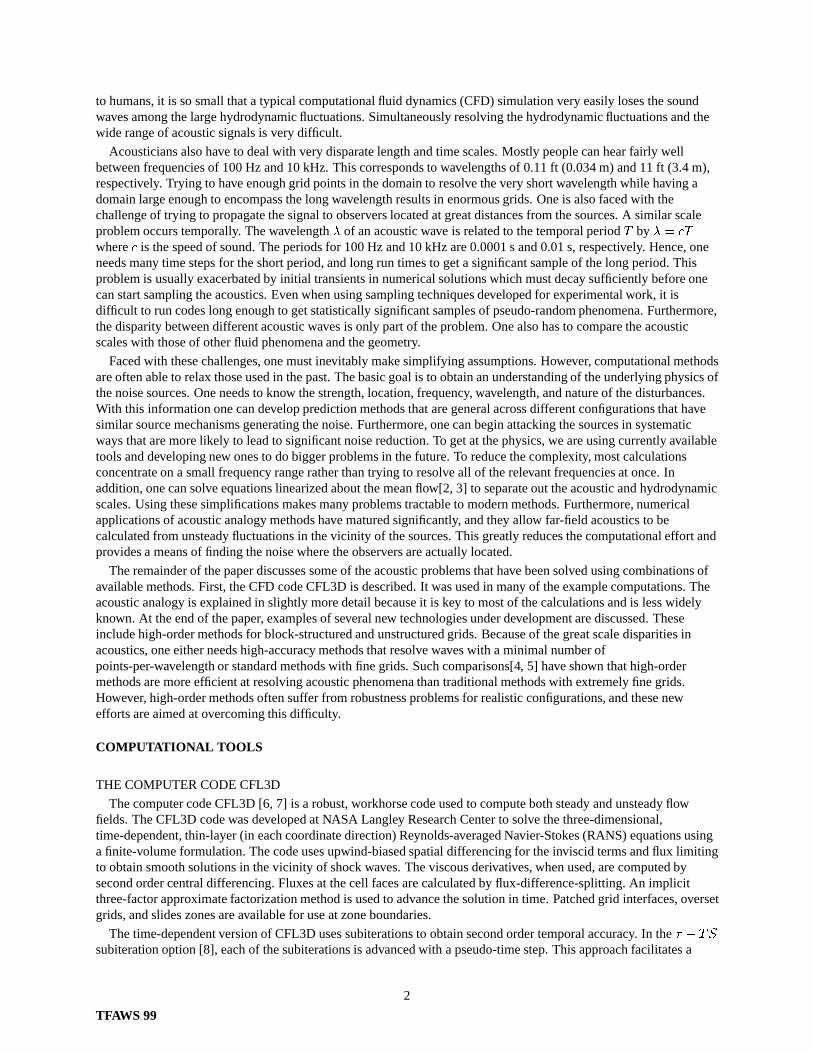
Figure 1. Comparison of measure and computed noise for a four-bladed Sikorsky model rotor. The microphonelocations was nominally 25 deg. below the rotor plane on the advancing side, 1.5 rotor radii from the rotor hub. This isa descent condition. (a) Measure time history; (b) predicted time history; (c) spectral comparison ( measured;� predicted)

Rotorcraft acoustics is an area where the FW-H equation has been utilized with great success. The codeWOPWOP[13] has been used extensively by industry and researchers to predict helicopter noise. Even for complexphenomena such as blade vortex interaction (BVI), WOPWOP correctly predicts the acoustic signature when it isgiven accurate pressure data as inputs. As an example, figure 1 compares the experimentally observed and computedacoustic signals[14] when experimentally measured surface pressures from a four bladed rotor where used as input toWOPWOP. The spectral comparison in figure 1 shows the agreement is good up to the 32nd harmonic. Similarcomparisons using CFD data as input do not yield such good results. This underscores the importance of havingaccurate input data on the integration surface. The acoustic theory is mature enough for such complicated problems,but more accurate CFD is needed.

SAMPLE APPLICATIONS

Although there are many problems that cannot be solved with conventional methods, appropriate assumptions canmake many realistic problems tractable. This section provides several examples where current methods weresuccessfully used to simulate important acoustic phenomena.

ROTOR NOISE

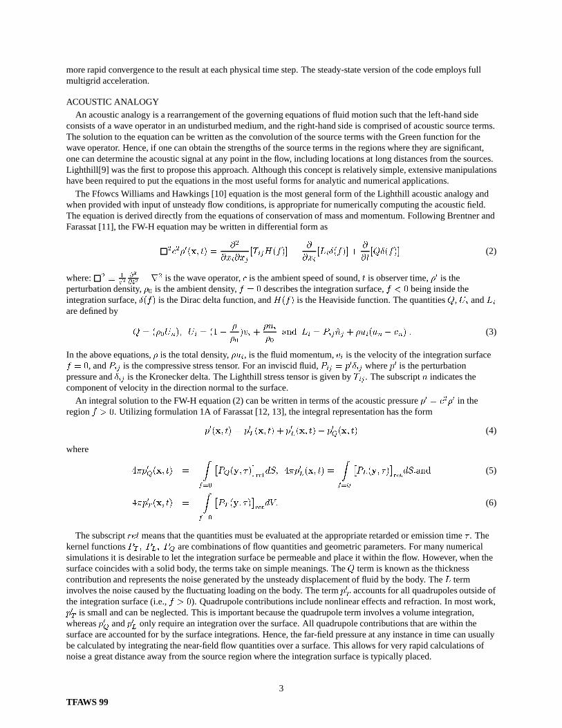
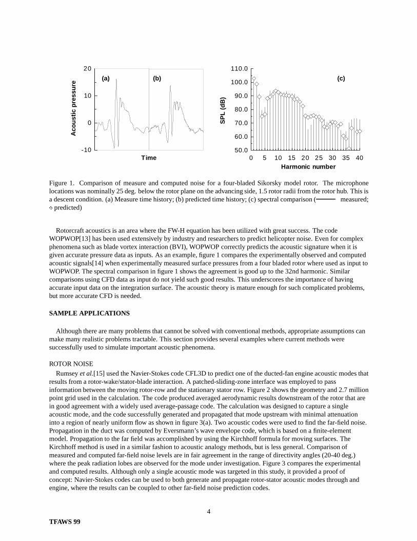
Rumseyet al.[15] used the Navier-Stokes code CFL3D to predict one of the ducted-fan engine acoustic modes thatresults from a rotor-wake/stator-blade interaction. A patched-sliding-zone interface was employed to passinformation between the moving rotor-row and the stationary stator row. Figure 2 shows the geometry and 2.7 millionpoint grid used in the calculation. The code produced averaged aerodynamic results downstream of the rotor that arein good agreement with a widely used average-passage code. The calculation was designed to capture a singleacoustic mode, and the code successfully generated and propagated that mode upstream with minimal attenuationinto a region of nearly uniform flow as shown in figure 3(a). Two acoustic codes were used to find the far-field noise.Propagation in the duct was computed by Eversmann’s wave envelope code, which is based on a finite-elementmodel. Propagation to the far field was accomplished by using the Kirchhoff formula for moving surfaces. TheKirchhoff method is used in a similar fashion to acoustic analogy methods, but is less general. Comparison ofmeasured and computed far-field noise levels are in fair agreement in the range of directivity angles (20-40 deg.)where the peak radiation lobes are observed for the mode under investigation. Figure 3 compares the experimentaland computed results. Although only a single acoustic mode was targeted in this study, it provided a proof ofconcept: Navier-Stokes codes can be used to both generate and propagate rotor-stator acoustic modes through andengine, where the results can be coupled to other far-field noise prediction codes.

4

TFAWS 99

(a) Geometry. (b) 2.7 million point grid.

Figure 2. Geometry and grid for rotor-wake/stator-blade interaction problem.

λ theory ∆x theory

(a) Near-field pressure. (b) Far-field noise.

Figure 3. Near-field pressure computed by CFL3D and far-field pressure computed by Eversmann’s wave envelopecode and a Kirchhoff technique.

5

TFAWS 99

(a) Vorticity Contours (b) Spectra

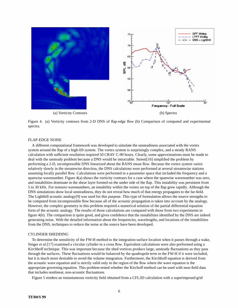
Figure 4. (a) Vorticity contours from 2-D DNS of flap-edge flow (b) Comparison of computed and experimentalspectra.

FLAP-EDGE NOISE

A different computational framework was developed to simulate the unsteadiness associated with the vortexsystem around the flap of a high-lift system. The vortex system is surprisingly complex, and a steady RANScalculation with sufficient resolution required 50 CRAY C-90 hours. Clearly, some approximations must be made todeal with the unsteady problem because a DNS would be intractable. Streett[16] simplified the problem byperforming a 2-D, incompressible DNS linearized about the RANS mean flow. Because the vortex system variesrelatively slowly in the streamwise direction, the DNS calculations were performed at several streamwise stationsassuming locally parallel flow. Calculations were performed in a parameter space that included the frequency and aspanwise wavenumber. Figure 4(a) shows the vorticity contours for a case where the spanwise wavenumber was zero,and instabilities dominate in the shear layer formed on the under side of the flap. This instability was persistent from5 to 30 kHz. For nonzero wavenumbers, an instability within the vortex on top of the flap grew rapidly. Although theDNS simulations show local unsteadiness, they do not reveal how much of that energy propagates to the far-field.The Lighthill acoustic analogy[9] was used for this purpose. This type of formulation allows the source strengths tobe computed from incompressible flow because all of the acoustic propagation is taken into account by the analogy.However, the complex geometry in this problem required a numerical solution of the partial differential equationform of the acoustic analogy. The results of those calculations are compared with those from two experiments infigure 4(b). The comparison is quite good, and gives confidence that the instabilities identified by the DNS are indeedgenerating noise. With the detailed information about the frequencies, wavelengths, and locations of the instabilitiesfrom the DNS, techniques to reduce the noise at the source have been developed.

CYLINDER SHEDDING

To determine the sensitivity of the FW-H method to the integration surface location when it passes through a wake,Singeret al.[17] examined a circular cylinder in a cross flow. Equivalent calculations were also performed using aKirchhoff technique. This was important because the shed vortices produce large, unsteady fluctuations as they passthrough the surfaces. These fluctuations would be balanced by the quadrupole term in the FW-H if it were included,but it is much more desirable to avoid the volume integration. Furthermore, the Kirchhoff equation is derived fromthe acoustic wave equation and is strictly valid only in the region of the flow where the wave equation is theappropriate governing equation. This problem tested whether the Kirchoff method can be used with near-field datathat includes nonlinear, non-acoustic fluctuations.

Figure 5 renders an instantaneous vorticity field obtained from a CFL3D calculation with a superimposed grid

6

TFAWS 99

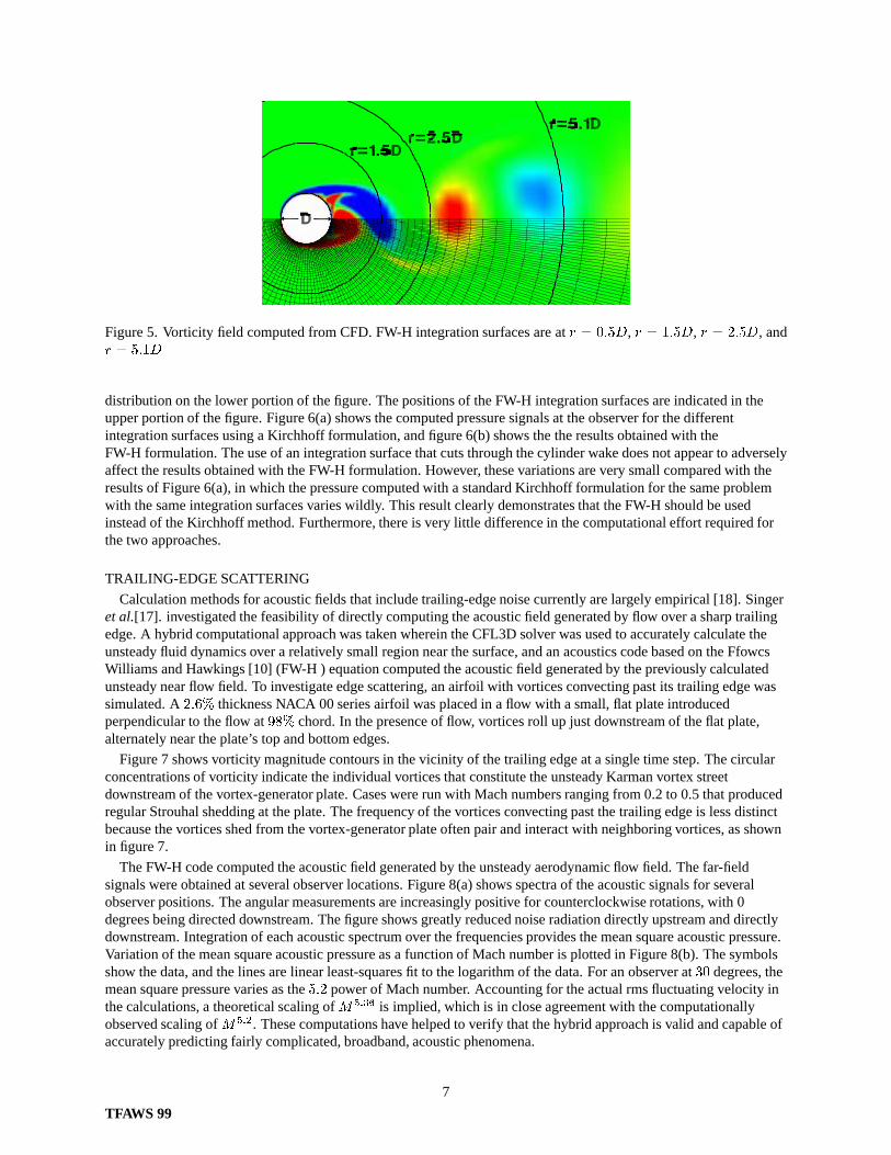
Figure 5. Vorticity field computed from CFD. FW-H integration surfaces are atr = 0:5D, r = 1:5D, r = 2:5D, andr = 5:1D

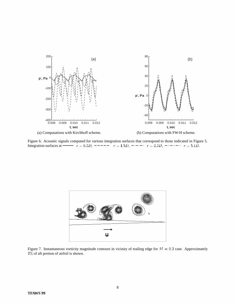
distribution on the lower portion of the figure. The positions of the FW-H integration surfaces are indicated in theupper portion of the figure. Figure 6(a) shows the computed pressure signals at the observer for the differentintegration surfaces using a Kirchhoff formulation, and figure 6(b) shows the the results obtained with theFW-H formulation. The use of an integration surface that cuts through the cylinder wake does not appear to adverselyaffect the results obtained with the FW-H formulation. However, these variations are very small compared with theresults of Figure 6(a), in which the pressure computed with a standard Kirchhoff formulation for the same problemwith the same integration surfaces varies wildly. This result clearly demonstrates that the FW-H should be usedinstead of the Kirchhoff method. Furthermore, there is very little difference in the computational effort required forthe two approaches.

TRAILING-EDGE SCATTERING

Calculation methods for acoustic fields that include trailing-edge noise currently are largely empirical [18]. Singeret al.[17]. investigated the feasibility of directly computing the acoustic field generated by flow over a sharp trailingedge. A hybrid computational approach was taken wherein the CFL3D solver was used to accurately calculate theunsteady fluid dynamics over a relatively small region near the surface, and an acoustics code based on the FfowcsWilliams and Hawkings [10] (FW-H ) equation computed the acoustic field generated by the previously calculatedunsteady near flow field. To investigate edge scattering, an airfoil with vortices convecting past its trailing edge wassimulated. A2:6% thickness NACA 00 series airfoil was placed in a flow with a small, flat plate introducedperpendicular to the flow at98% chord. In the presence of flow, vortices roll up just downstream of the flat plate,alternately near the plate’s top and bottom edges.

Figure 7 shows vorticity magnitude contours in the vicinity of the trailing edge at a single time step. The circularconcentrations of vorticity indicate the individual vortices that constitute the unsteady Karman vortex streetdownstream of the vortex-generator plate. Cases were run with Mach numbers ranging from 0.2 to 0.5 that producedregular Strouhal shedding at the plate. The frequency of the vortices convecting past the trailing edge is less distinctbecause the vortices shed from the vortex-generator plate often pair and interact with neighboring vortices, as shownin figure 7.

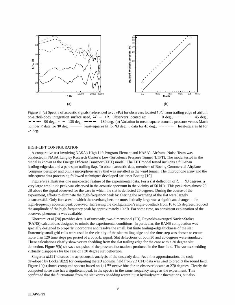
The FW-H code computed the acoustic field generated by the unsteady aerodynamic flow field. The far-fieldsignals were obtained at several observer locations. Figure 8(a) shows spectra of the acoustic signals for severalobserver positions. The angular measurements are increasingly positive for counterclockwise rotations, with 0degrees being directed downstream. The figure shows greatly reduced noise radiation directly upstream and directlydownstream. Integration of each acoustic spectrum over the frequencies provides the mean square acoustic pressure.Variation of the mean square acoustic pressure as a function of Mach number is plotted in Figure 8(b). The symbolsshow the data, and the lines are linear least-squares fit to the logarithm of the data. For an observer at30 degrees, themean square pressure varies as the5:2 power of Mach number. Accounting for the actual rms fluctuating velocity inthe calculations, a theoretical scaling ofM5:36 is implied, which is in close agreement with the computationallyobserved scaling ofM5:2. These computations have helped to verify that the hybrid approach is valid and capable ofaccurately predicting fairly complicated, broadband, acoustic phenomena.

7

TFAWS 99

0.008 0.009 0.010 0.011 0.012-400

-300

-200

-100

0

100

200

t, sec

p′, Pa

(a)

(a) Computations with Kirchhoff scheme.

0.008 0.009 0.010 0.011 0.012

-40

-20

0

20

40

60

80

p′, Pa

t, sec

(b)

(b) Computations with FW-H scheme.

Figure 6. Acoustic signals computed for various integration surfaces that correspond to those indicated in Figure 5.Integration surfaces at r = 0:5D, r = 1:5D, r = 2:5D, r = 5:1D.

Figure 7. Instantaneous vorticity magnitude contours in vicinity of trailing edge forM = 0:2 case. Approximately2% of aft portion of airfoil is shown.

8

TFAWS 99

10000 20000 30000f, Hz

10

20

30

40

50

60

70S

PL

,dB

(a)

0.2 0.25 0.3 0.35 0.4 0.45Mach

10

20

30

40506070

squa

red

aco

ustic

pre

ssu

re,P

a2

(b)

Figure 8. (a) Spectra of acoustic signals (referenced to20�Pa) for observers located10C from trailing edge of airfoil;on-airfoil-body integration surface used,M = 0:2. Observers located at: 0 deg., 45 deg.,

90 deg., 135 deg., 180 deg. (b) Variation in mean square acoustic pressure versus Machnumber; data for30 deg., least-squares fit for30 deg.,� data for45 deg., least-squares fit for45 deg.

HIGH-LIFT CONFIGURATION

A cooperative test involving NASA’s High-Lift Program Element and NASA’s Airframe Noise Team wasconducted in NASA Langley Research Center’s Low-Turbulence Pressure Tunnel (LTPT). The model tested in thetunnel is known as the Energy Efficient Transport (EET) model. The EET model tested includes a full-spanleading-edge slat and a part-span trailing flap. To obtain acoustic data, members of Boeing Commercial AirplaneCompany designed and built a microphone array that was installed in the wind tunnel. The microphone array and thesubsequent data processing followed techniques developed earlier at Boeing [19].

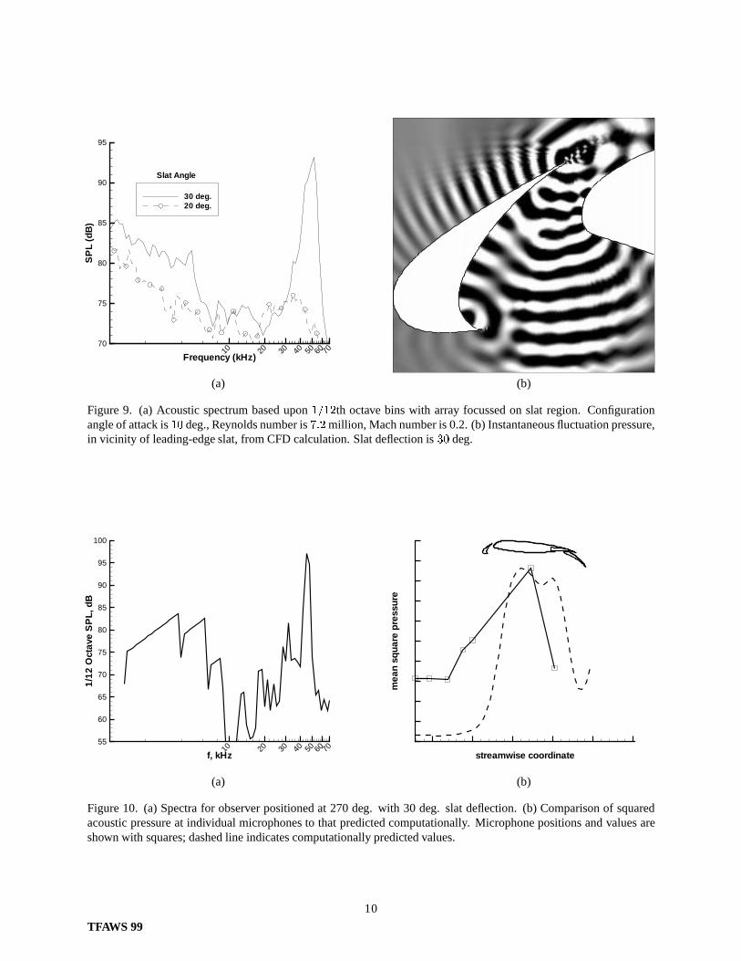
Figure 9(a) illustrates one unexpected feature of the experimental data. For a slat deflection of�s = 30 degrees, avery large amplitude peak was observed in the acoustic spectrum in the vicinity of 50 kHz. This peak rises almost 20dB above the signal observed for the case in which the slat is deflected 20 degrees. During the course of theexperiment, efforts to eliminate the high-frequency peak by altering the overhang of the slat were largelyunsuccessful. Only for cases in which the overhang became unrealistically large was a significant change in thehigh-frequency acoustic peak observed. Increasing the configuration’s angle-of-attack from 10 to 15 degrees, reducedthe amplitude of the high-frequency peak by approximately 10 dB. For some time, no consistent explanation of theobserved phenomena was available.

Khorrami et al [20] provides details of unsteady, two-dimensional (2D), Reynolds-averaged Navier-Stokes(RANS) calculations designed to mimic the experimental conditions. In particular, the RANS computation wasspecially designed to properly incorporate and resolve the small, but finite trailing-edge thickness of the slat.Extremely small grid cells were used in the vicinity of the slat trailing edge and the time step was chosen to ensuremore than 120 time steps per period of a 50 kHz signal. Slat deflections of both 30 and 20 degrees were simulated.These calculations clearly show vortex shedding from the slat trailing edge for the case with a 30 degree slatdeflection. Figure 9(b) shows a snapshot of the pressure fluctuations produced in the flow field. The vortex sheddingvirtually disappears for the case of a 20 degree slat deflection.

Singeret al.[21] discuss the aeroacoustic analysis of the unsteady data. As a first approximation, the codedeveloped by Lockard[22] for computing the 2D acoustic field from 2D CFD data was used to predict the sound field.Figure 10(a) shows computed spectra based on1=12th octave bins for an observer located at 270 degrees. Clearly thecomputed noise also has a significant peak in the spectra in the same frequency range as the experiment. Thisconfirmed that the fluctuations from the slat vortex shedding weren’t just hydrodynamic fluctuations, but also

9

TFAWS 99

10 20 30 40 50 60 70Frequency (kHz)

70

75

80

85

90

95

SP

L(d

B)

30 deg.20 deg.

Slat Angle

(a) (b)

Figure 9. (a) Acoustic spectrum based upon1=12th octave bins with array focussed on slat region. Configurationangle of attack is10 deg., Reynolds number is7:2 million, Mach number is 0.2. (b) Instantaneous fluctuation pressure,in vicinity of leading-edge slat, from CFD calculation. Slat deflection is30 deg.

f, kHz

1/1

2O

ctav

eS

PL,

dB

10 20 30 40 50 60 7055

60

65

70

75

80

85

90

95

100

(a)

streamwise coordinate

mea

nsq

uare

pres

sure

(b)

Figure 10. (a) Spectra for observer positioned at 270 deg. with 30 deg. slat deflection. (b) Comparison of squaredacoustic pressure at individual microphones to that predicted computationally. Microphone positions and values areshown with squares; dashed line indicates computationally predicted values.

10

TFAWS 99

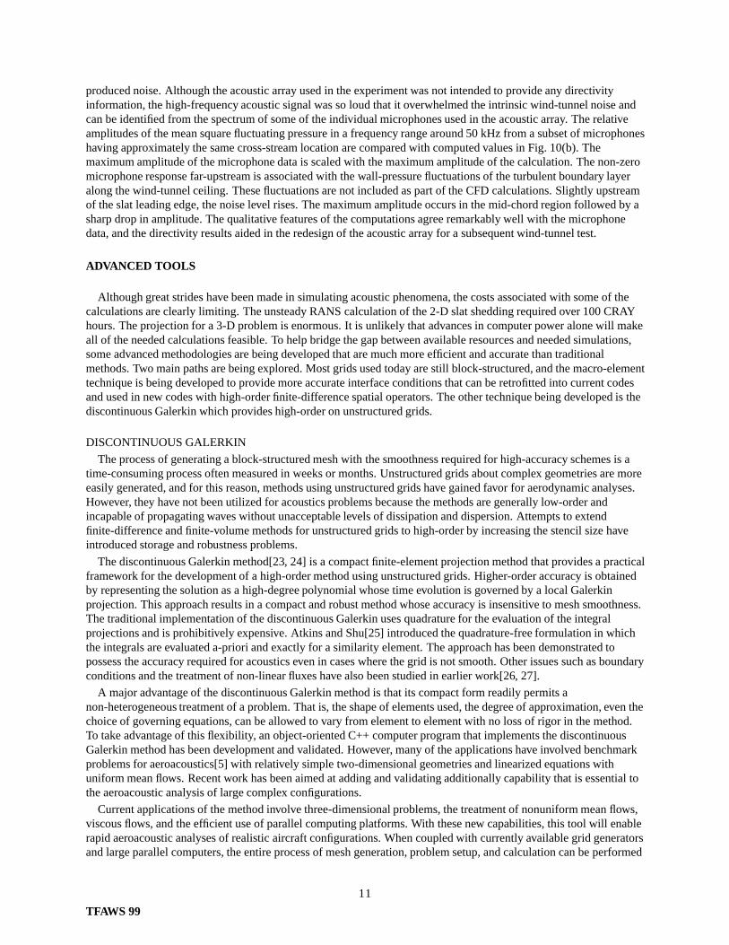
produced noise. Although the acoustic array used in the experiment was not intended to provide any directivityinformation, the high-frequency acoustic signal was so loud that it overwhelmed the intrinsic wind-tunnel noise andcan be identified from the spectrum of some of the individual microphones used in the acoustic array. The relativeamplitudes of the mean square fluctuating pressure in a frequency range around 50 kHz from a subset of microphoneshaving approximately the same cross-stream location are compared with computed values in Fig. 10(b). Themaximum amplitude of the microphone data is scaled with the maximum amplitude of the calculation. The non-zeromicrophone response far-upstream is associated with the wall-pressure fluctuations of the turbulent boundary layeralong the wind-tunnel ceiling. These fluctuations are not included as part of the CFD calculations. Slightly upstreamof the slat leading edge, the noise level rises. The maximum amplitude occurs in the mid-chord region followed by asharp drop in amplitude. The qualitative features of the computations agree remarkably well with the microphonedata, and the directivity results aided in the redesign of the acoustic array for a subsequent wind-tunnel test.

ADVANCED TOOLS

Although great strides have been made in simulating acoustic phenomena, the costs associated with some of thecalculations are clearly limiting. The unsteady RANS calculation of the 2-D slat shedding required over 100 CRAYhours. The projection for a 3-D problem is enormous. It is unlikely that advances in computer power alone will makeall of the needed calculations feasible. To help bridge the gap between available resources and needed simulations,some advanced methodologies are being developed that are much more efficient and accurate than traditionalmethods. Two main paths are being explored. Most grids used today are still block-structured, and the macro-elementtechnique is being developed to provide more accurate interface conditions that can be retrofitted into current codesand used in new codes with high-order finite-difference spatial operators. The other technique being developed is thediscontinuous Galerkin which provides high-order on unstructured grids.

DISCONTINUOUS GALERKIN

The process of generating a block-structured mesh with the smoothness required for high-accuracy schemes is atime-consuming process often measured in weeks or months. Unstructured grids about complex geometries are moreeasily generated, and for this reason, methods using unstructured grids have gained favor for aerodynamic analyses.However, they have not been utilized for acoustics problems because the methods are generally low-order andincapable of propagating waves without unacceptable levels of dissipation and dispersion. Attempts to extendfinite-difference and finite-volume methods for unstructured grids to high-order by increasing the stencil size haveintroduced storage and robustness problems.

The discontinuous Galerkin method[23, 24] is a compact finite-element projection method that provides a practicalframework for the development of a high-order method using unstructured grids. Higher-order accuracy is obtainedby representing the solution as a high-degree polynomial whose time evolution is governed by a local Galerkinprojection. This approach results in a compact and robust method whose accuracy is insensitive to mesh smoothness.The traditional implementation of the discontinuous Galerkin uses quadrature for the evaluation of the integralprojections and is prohibitively expensive. Atkins and Shu[25] introduced the quadrature-free formulation in whichthe integrals are evaluated a-priori and exactly for a similarity element. The approach has been demonstrated topossess the accuracy required for acoustics even in cases where the grid is not smooth. Other issues such as boundaryconditions and the treatment of non-linear fluxes have also been studied in earlier work[26, 27].

A major advantage of the discontinuous Galerkin method is that its compact form readily permits anon-heterogeneous treatment of a problem. That is, the shape of elements used, the degree of approximation, even thechoice of governing equations, can be allowed to vary from element to element with no loss of rigor in the method.To take advantage of this flexibility, an object-oriented C++ computer program that implements the discontinuousGalerkin method has been development and validated. However, many of the applications have involved benchmarkproblems for aeroacoustics[5] with relatively simple two-dimensional geometries and linearized equations withuniform mean flows. Recent work has been aimed at adding and validating additionally capability that is essential tothe aeroacoustic analysis of large complex configurations.

Current applications of the method involve three-dimensional problems, the treatment of nonuniform mean flows,viscous flows, and the efficient use of parallel computing platforms. With these new capabilities, this tool will enablerapid aeroacoustic analyses of realistic aircraft configurations. When coupled with currently available grid generatorsand large parallel computers, the entire process of mesh generation, problem setup, and calculation can be performed

11

TFAWS 99

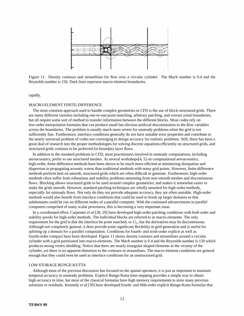
Figure 11. Density contours and streamlines for flow over a circular cylinder. The Mach number is 0.4 and theReynolds number is 150. Dark lines represent macro-element boundaries.

rapidly.

MACRO-ELEMENT FINITE-DIFFERENCE

The most common approach used to handle complex geometries in CFD is the use of block-structured grids. Thereare many different varieties including one-to-one point matching, arbitrary patching, and overset zonal boundaries,but all require some sort of method to transfer information between the different blocks. Most codes rely onlow-order interpolation formulas that can produce small but obvious artificial discontinuities in the flow variablesacross the boundaries. The problem is usually much more severe for unsteady problems when the grid is notsufficiently fine. Furthermore, interface conditions generally do not have suitable error properties and contribute tothe nearly universal problem of codes not converging to design accuracy for realistic problems. Still, there has been agreat deal of research into the proper methodologies for solving discrete equations efficiently on structured grids, andstructured grids continue to be preferred for boundary layer flows.

In addition to the standard problems in CFD, most practitioners involved in unsteady computations, includingaeroacoustics, prefer to use structured meshes. At several workshops[4, 5] on computational aeroacoustics,high-order, finite-difference methods have been shown to be much more efficient at minimizing dissipation anddispersion in propagating acoustic waves than traditional methods with many grid points. However, finite-differencemethods perform best on smooth, structured grids which are often difficult to generate. Furthermore, high-ordermethods often suffer from robustness and stability problems stemming from non-smooth meshes and discontinuousflows. Blocking allows structured grids to be used around complex geometries, and makes it somewhat easier tomake the grids smooth. However, standard patching techniques are wholly unsuited for high-order methods,especially for unsteady flows. Not only do they not provide adequate accuracy, they are often unstable. High-ordermethods would also benefit from interface conditions that could be used to break up larger domains so thatsubdomains could be run on different nodes of a parallel computer. With the continued advancements in parallelcomputers comprised of many scalar processors, this is becoming a very important issue.

In a coordinated effort, Carpenteret al.[28, 29] have developed high-order patching conditions with both order andstability proofs for high-order methods. The individual blocks are referred to as macro-elements. The onlyrequirement for the grid is that the interface be point matched, orC0, but the derivatives may be discontinuous.Although not completely general, it does provide some significant flexibility in grid generation and is useful forsplitting up a domain for a parallel computation. Conditions for fourth- and sixth-order explicit as well asfourth-order compact have been developed. Figure 11 shows density contours and streamlines around a circularcylinder with a grid partitioned into macro-elements. The Mach number is 0.4 and the Reynolds number is 150 whichproduces strong vortex shedding. Notice that there are nearly triangular shaped elements in the vicinity of thecylinder, yet there is no apparent distortion to the contours or streamlines. The macro-element conditions are generalenough that they could even be used as interface conditions for an unstructured grid.

LOW-STORAGE RUNGE-KUTTA

Although most of the previous discussion has focused on the spatial operators, it is just as important to maintaintemporal accuracy in unsteady problems. Explicit Runge-Kutta time-stepping provides a simple way to obtainhigh-accuracy in time, but most of the classical formulas have high memory requirements to store many previoussolutions or residuals. Kennedyet al.[30] have developed fourth- and fifth-order explicit Runge-Kutta formulas that

12

TFAWS 99

only require2N storage forN unknowns. This can be a substantial savings in memory, and can also be verybeneficial in the run time on cache-based computers which are often limited by memory access. Furthermore, some ofthe new Runge-Kutta methods have embedded lower-order formulas that allow for automated time-stepping by usingthe solutions from the two orders to determine if there is too much error and the time step needs to be decreased.

A difficulty with explicit time stepping for unsteady problems is that the time step must be chosen to keep thesmallest cell in the entire grid stable. In boundary layer flows with strong clustering towards walls, this can result in atime-step orders of magnitude smaller than what is needed for temporal accuracy. Research is ongoing into differentimplicit methods that can be used in regions where the grid spacing is extremely small.

SUMMARY

Despite the simplifications used in the examples, the cost of performing many of the acoustic calculations was stillvery high. Just obtaining a highly resolved mean flow for a high-lift flap system required 50 CRAY C-90 hours, andan unsteady RANS of a two-dimensional slat problem required over 100 hours. Nonetheless, some significant insighthas been gained by applying currently available computational techniques to problems of interest. Typically, thecalculations concentrated on resolving certain frequency ranges rather than trying to solve for all of the scalessimultaneously. Because many important noise sources are narrow band, this approach is appropriate. The noisegenerated from vortex-shedding at a slat trailing edge is a good example in which this approach was taken, and apreviously unknown noise source was identified. There remain many problems that cannot be solved today, and someof the efforts at NASA Langley to develop advanced tools that will enable the next generation of acoustic simulationshave been highlighted.

ACKNOWLEDGMENTS

The author would like to thank the members of the Computational Modeling and Simulation Branch at NASALangley Research Center for their significant contributions to this paper.

REFERENCES

1. W. R. WATSON, M. G. JONES, S. E. TANNER and T. L. PARROTT 1996AIAA Journal34(3), 548–554.Validation of a numerical method for extracting liner impedance.

2. P. J. MORRIS, Q. WANG, L. N. LONG and D. P. LOCKARD 1997AIAA Paper No.97-1598. Numericalpredictions of high-speed jet noise.

3. J. C. HARDIN and D. S. POPE1994Theoretical and Computational Physics6(5-6). An acoustic/viscoussplitting technique for computational aeroacoustics.

4. J. C. Hardin and M. Y. Hussaini, editors 1993Computational Aeroacoustics. Springer-Verlag. (Presentations atthe Workshop on Computational Aeroacoustics sponsored by ICASE and the acoustics division of NASA LaRCon April 6-9.)

5. C. K. W. Tam and J. C. Hardin, editors 1997Second Computational Aeroacoustics (CAA) Workshop onBenchmark Problems. NASA CP-3352. (Proceedings of a workshop sponsored by NASA and Florida StateUniversity in Tallahassee, Florida on Nov. 4-5, 1996.)

6. C. RUMSEY, R. BIEDRON and J. THOMAS 1997TM 112861. NASA. (presented at the Godonov’s Method forGas Dynamics Symposium, Ann Arbor, MI.) CFL3D: Its history and some recent applications.

7. S. L. KRIST, R. T. BIEDRON and C. RUMSEY 1997. NASA Langley Research Center, Aerodynamic andAcoustic Methods Branch.CFL3D User’s Manual (Version 5).

8. C. L. RUMSEY, M. D. SANETRIK, R. T. BIEDRON, N. D. MELSON and E. B. PARLETTE 1996Computersand Fluids25(2), 217–236. Efficiency and accuracy of time-accurate turbulent Navier-Stokes computations.

9. M. J. LIGHTHILL 1952Proceedings of the Royal SocietyA221, 564–587. On sound generatedaerodynamically, I: general theory.

13

TFAWS 99

10. J. E. FFOWCSWILLIAMS and D. L. HAWKINGS 1969Philosophical Transactions of the Royal SocietyA264(1151), 321–342. Sound generated by turbulence and surfaces in arbitrary motion.

11. K. S. BRENTNERand F. FARASSAT 1998AIAA Journal36(8), 1379–1386. An analytical comparison of theacoustic analogy and kirchhoff formulation for moving surfaces.

12. F. FARASSAT and G. P. SUCCI 19883Vertica7(4), 309–320. The prediction of helicopter discrete frequencynoise.

13. K. S. BRENTER1986. NASA Langley Research Center. (NASA TM 87721.),Prediction of Helicopter DiscreteFrequency Rotor Noise – A Computer Program Incorporating Realistic Blade Motions and AdvancedFormulation

14. K. S. BRENTNERand F. FARASSAT 1994Journal of Sound and Vibration170(1), 79–96. Helicopter noiseprediction: The current status and future direction.

15. C. L. RUMSEY, R. BIEDRON, F. FARASSAT and P. L. SPENCE1998Journal of Sound and Vibration213(4),643–664. Ducted-fan engine acoustic predictions using a Navier-Stokes code.

16. C. L. STREETT1998AIAA Paper No.98-2226. Numerical simulation of a flap-edge flowfield.

17. B. A. SINGER, K. S. BRENTNER, D. L. LOCKARD and G. M. LILLEY 1999AIAA Paper No.99-0231.Simulation of acoustic scattering from a trailing edge.

18. S. WAGNER, R. BAREISSand G. GUIDATI 1996Wind Turbine Noise. New York: Springer.

19. J. R. UNDERBRINK and R. P. DOUGHERTY 1996NOISECON 96. Array design for non-intrusive measurmentsof noise sources.

20. M. R. KHORRAMI, M. E. BERKMAN, M. CHOUDHARI, B. A. SINGER, D. L. LOCKARD and K. S.BRENTNER1999AIAA Paper No.99-1805. Unsteady flow computations of a slat with a blunt trailing edge.

21. B. A. SINGER, D. L. LOCKARD, K. S. BRENTNER, M. R. KHORRAMI, M. E. BERKMAN andM. CHOUDHARI 1999AIAA Paper No.99-1802. Computational acoustic analysis of slat trailing-edge flow.

22. D. P. LOCKARD. (to appear injournal of sound and vibration.) An efficient, two-dimensional implementationof the Ffowcs Williams and Hawkings equation.

23. C. JOHNSONand J. PITKARATA 1986Mathematics of Computation46(176), 1–26. An analysis of thediscontinuous Galerkin method for a scalar hyperbolic equation.

24. B. COCKBURN and C.-W. SHU 1998SIAM Journal of Numerical Analysis35, 2440–2463. The localdiscontinuous Galerkin method for time-dependent convection-diffusion systems.

25. H. L. ATKINS and C. W. SHU 1997AIAA Journal36(5), 775–782. Quadrature-free implementation ofdiscontinuous Galerkin method for hyperbolic equations.

26. H. L. ATKINS 1997. AIAA Paper-97-1581. (Third Joint CEAS/AIAA Aeroacoustics Conference, May 12-14.)Continued development of the discontinuous Galerkin method for computational aeroacoustic applications.

27. H. L. ATKINS 1997. AIAA Paper 97-2032. (13th AIAA computational fluid dynamics conference, SnowmassVillage, Colorado, June 29-July 2.) Local analysis of shock capturing using discontinuous Galerkinmethodology.

28. M. H. CARPENTER, J. NORDSTROMand D. GOTTLEIB 1999Journal of Computational Physics148,341–365. A stable and conservative interface treatment of arbitrary spatial accuracy.

29. M. H. CARPENTERand J. NORDSTROM1999Journal of Computational Physics148, 621–645. Boundary andinterface conditions for high-order finite-difference methods applied to the Euler and Navier-Stokes equations.

30. C. A. KENNEDY, M. H. CARPENTERand R. LEWIS. (to appear inapplied numerical mathematics.)Low-storage explicit Runge-Kutta schemes for the compressible Navier-Stokes equations.

14

TFAWS 99