Aerothermodynamics of High Speed Flows - uliege.be · AERO0033-1, Aerothermodynamics of High Speed Flows, Lecture 1 The sound barrier • Control reversal: Airfoil centreof pressure

AERO0033-1, Aerothermodynamics of High Speed Flows, Lecture 1

Lecture 1:Introduction G. Dimitriadis

Aerothermodynamics of High Speed Flows

1


The sound barrier• Supersonic aerodynamics and aircraft design

go hand in hand• Aspects of supersonic flow theory were

developed in the late 19th and early 20th

century• These remained mostly subjects of academic

interest until the 1940s.• As aircraft flight speed kept increasing pilots

started experiencing weird phenomena.

2


The sound barrier• Control reversal: Airfoil centre of pressure position

changes at high airspeed. Moments around the flexural axis become very important causing aeroelastic twisting of wings. The end result can be a reversal of the effect of control deflections.

• Sudden drag increases: shock waves form on the suction side of wings and can increase the drag significantly

• Shock-induced flutter/buffetting: shock waves on wings and control surfaces can oscillate causing vibrations. Small amplitude versions of this phenomenon are known as transonic buzz.

3


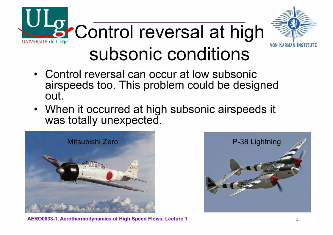
Control reversal at highsubsonic conditions

4

Mitsubishi Zero P-38 Lightning

• Control reversal can occur at low subsonic airspeeds too. This problem could be designed out.

• When it occurred at high subsonic airspeeds it was totally unexpected.


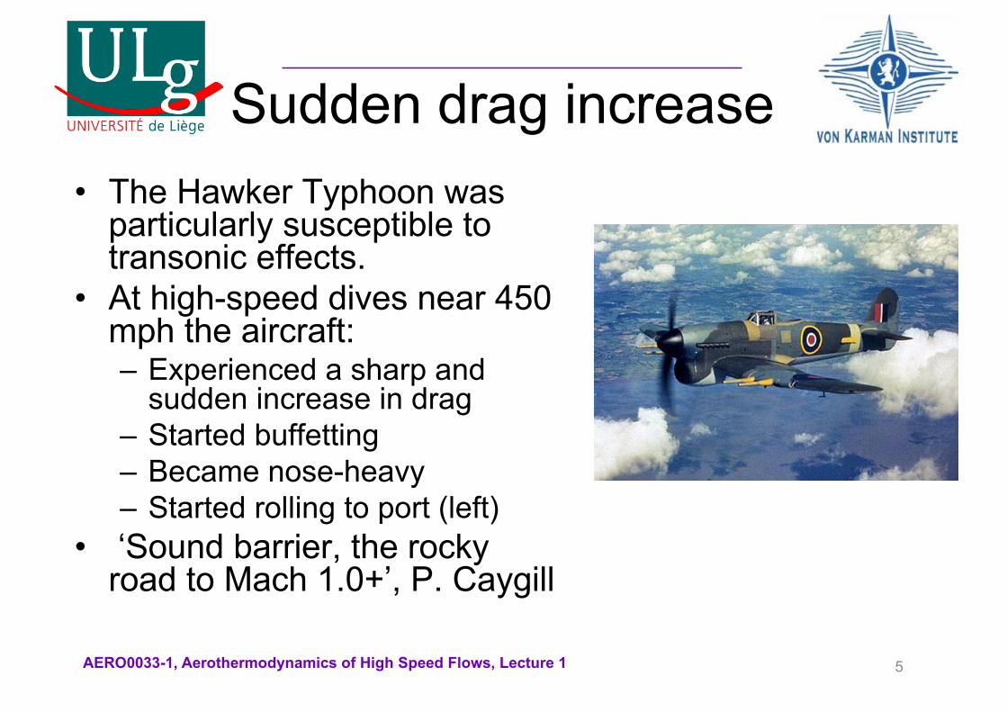
Sudden drag increase• The Hawker Typhoon was

particularly susceptible to transonic effects.

• At high-speed dives near 450 mph the aircraft:– Experienced a sharp and

sudden increase in drag– Started buffetting– Became nose-heavy– Started rolling to port (left)

• ‘Sound barrier, the rocky road to Mach 1.0+’, P. Caygill

5


Transonic buzz• Usually appears as a vibration in the

control surfaces (aileron, elevator, elevonetc)

6

1941: ‘My speedometer was soon … topping the 1000 km/h mark. … there was a sudden vibration in the elevonsand … the aircraft went into an uncontrollable dive, causing high negative g. I immediately cut the rocket … Just as suddenly the controls reacted normally again and I eased the aircraft out of its dive.’

Heini Dittmar


What speed?• Transonic effects appeared at different flight

conditions for different aircraft.• The Me-163 started experiencing transonic effects at

M=0.84• The P-38 Lightning at M=0.68• The Hawker Typhoon at M=0.64• ‘History of Shock Waves, Explosions and Impact’,

P.O.K. Krehl• In the end the sound barrier was not a physical

phenomenon.• It was the experience of a collection of unfavourable

phenomena at high subsonic airspeeds.

7


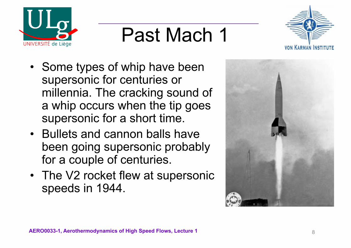
Past Mach 1• Some types of whip have been

supersonic for centuries or millennia. The cracking sound of a whip occurs when the tip goes supersonic for a short time.

• Bullets and cannon balls have been going supersonic probably for a couple of centuries.

• The V2 rocket flew at supersonic speeds in 1944.

8


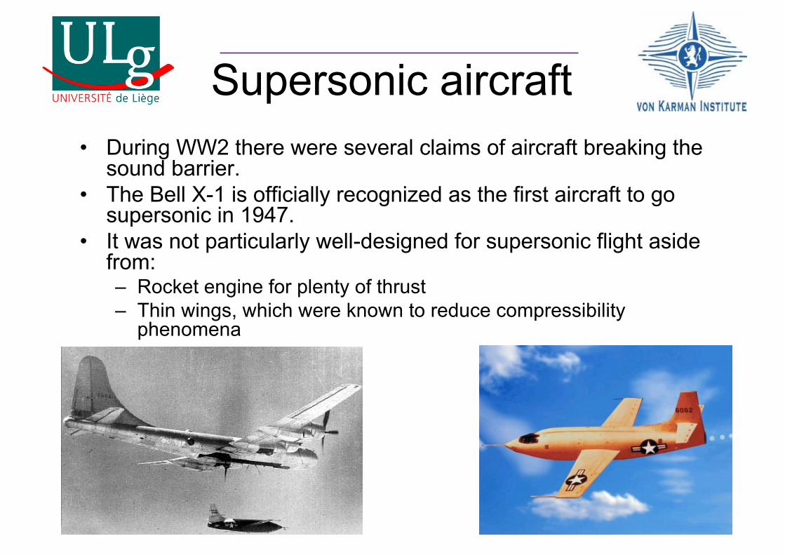
Supersonic aircraft• During WW2 there were several claims of aircraft breaking the

sound barrier.• The Bell X-1 is officially recognized as the first aircraft to go

supersonic in 1947.• It was not particularly well-designed for supersonic flight aside

from:– Rocket engine for plenty of thrust– Thin wings, which were known to reduce compressibility

phenomena

9


Faster than supersonic• Flight conditions at M>4 are conventionally

known as hypersonic.• A US variant of the V-2 rocket reached Mach

5 in 1949.• As the space age dawned, hypersonic flight

became increasingly frequent.• Yuri Gagarin was the first human to fly at

hypersonic conditions.• Atmospheric reentry occurs almost always at

hypersonic flight conditions.

10


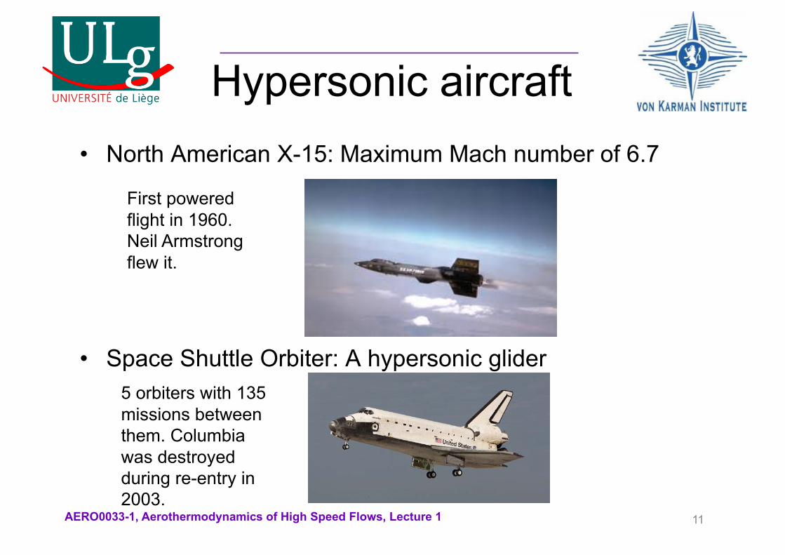
Hypersonic aircraft• North American X-15: Maximum Mach number of 6.7

• Space Shuttle Orbiter: A hypersonic glider

11

First powered flight in 1960. Neil Armstrong flew it.

5 orbiters with 135 missions between them. Columbia was destroyed during re-entry in 2003.


Aims of this course• Present and discuss the physics of

transonic, supersonic and hypersonic flight.

• Develop the fluid equations at different flight regimes and discuss solution methods.

• Detail how the theory has been applied to aircraft and discuss engineering solutions to unfavorable phenomena.

12


Teaching material• The main textbook for this course is:

– Modern Compressible Flow with Historical Perspective, J. D. Anderson, Third Edition, McGraw-Hill, 2004

• Students are not required to buy the book. The lecture notes should be sufficient.

• Pdfs of the Powerpoint presentations will be available at: – http://www.ltas-

aea.ulg.ac.be/cms/index.php?page=supersonic-course• Lecture attendance is highly recommended, not all the

course material is covered in the pdfs.

13


Practical sessions• Practical sessions will include:

– Class examples– One experimental session at the Von Karman

Institute– One piece of coursework on transonic

simulation• The students will submit reports on their

experimental and simulation work.

14


Assessment• Student assessment will be based on the

following:– An oral exam in the May-June exam session

(60% of the grade)– Assessment of the report on the experimental

work (20% of the grade)– Assessment of the report on the practical

work (20% of the grade)

15


Compressible fluids• Compressible flow is one where the

density of the fluid is not constant; it can change in time and space.

• All fluids are compressible to a certain amount, although gases are much more easily compressed than liquids.

• Compressibility defines how easy it is to change the density of a fluid.

16


Compressibility• Consider a small moving fluid element:

• Its density if r while the pressure exerted on it by the fluid particles around it is p.

• If the pressure exerted on the element is increased by dp, its density will increase by dr.

• Compressibility is defined as:

17

p

r

p

pp

τ =1ρdρdp


Compressibility (2)• Therefore compressibility is the percentage

change in density of a fluid element due to a small change in pressure acting on the element.

• Compressibility has units of 1/Pa, or m2/N.• Note that the density of a gas can change even if

the pressure is constant, due to changes in temperature.

• Usually two types of compressibility are quoted:– Compressibility at constant temperature– Compressibility at constant entropy (i.e. no heat

addition)

18


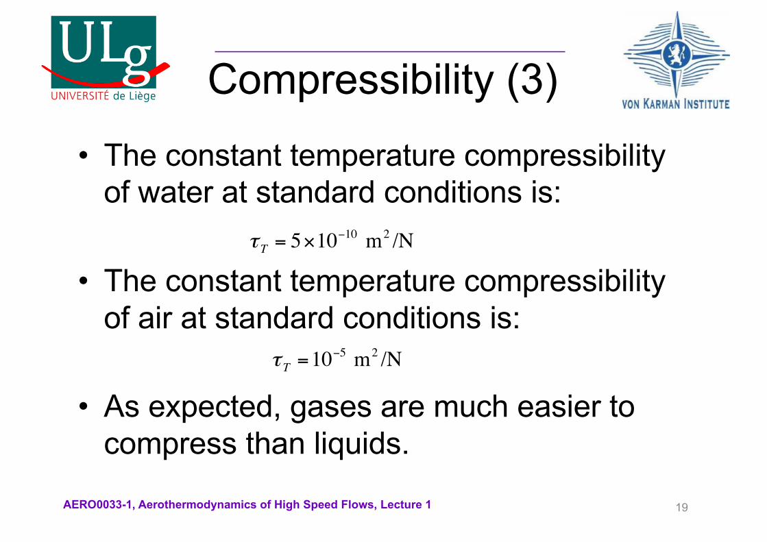
Compressibility (3)• The constant temperature compressibility

of water at standard conditions is:

• The constant temperature compressibility of air at standard conditions is:

• As expected, gases are much easier to compress than liquids.

19

τ T = 5×10−10 m2 /N

τ T =10−5 m2 /N


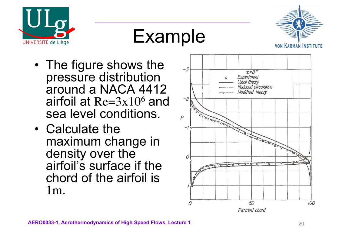
Example• The figure shows the

pressure distribution around a NACA 4412 airfoil at Re=3x106 and sea level conditions.

• Calculate the maximum change in density over the airfoil’s surface if the chord of the airfoil is 1m.

20


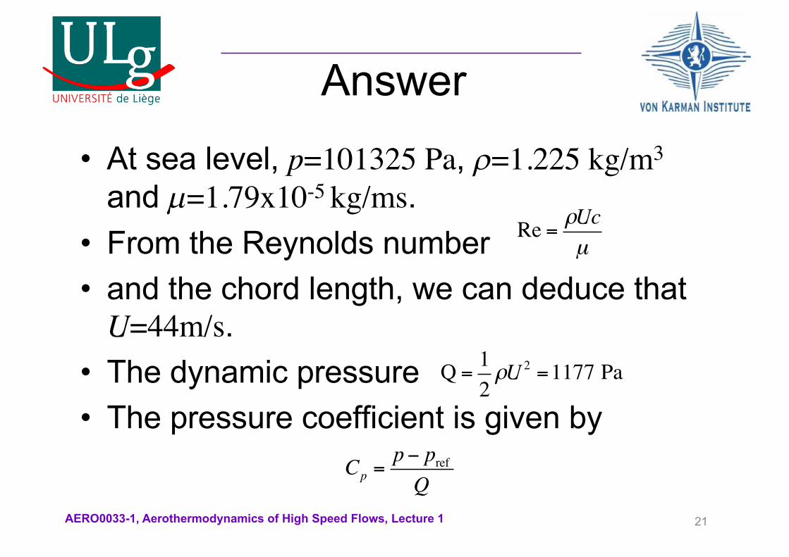
Answer• At sea level, p=101325 Pa, r=1.225 kg/m3

and µ=1.79x10-5 kg/ms.• From the Reynolds number • and the chord length, we can deduce that

U=44m/s.• The dynamic pressure • The pressure coefficient is given by

21

Re = ρUcµ

Cp =p− prefQ

Q =12ρU 2 =1177 Pa


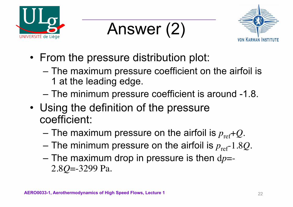
Answer (2)• From the pressure distribution plot:

– The maximum pressure coefficient on the airfoil is 1 at the leading edge.

– The minimum pressure coefficient is around -1.8.• Using the definition of the pressure

coefficient:– The maximum pressure on the airfoil is pref+Q.– The minimum pressure on the airfoil is pref-1.8Q.– The maximum drop in pressure is then dp=-

2.8Q=-3299 Pa.

22


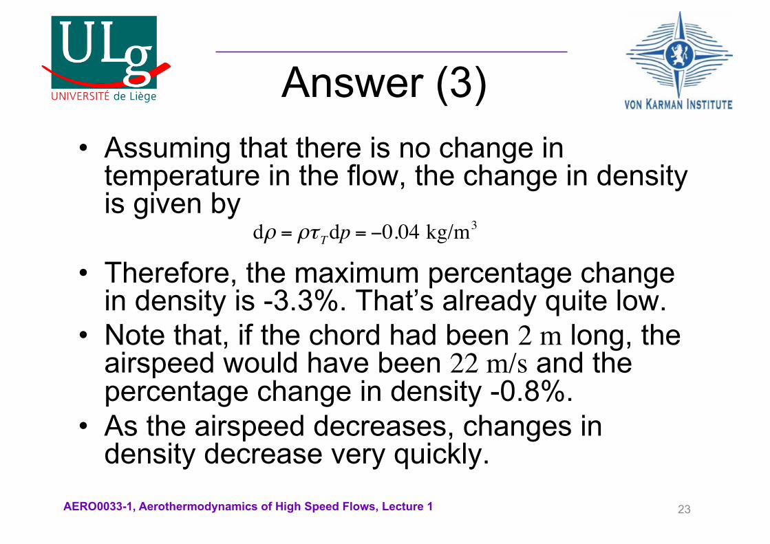
Answer (3)• Assuming that there is no change in

temperature in the flow, the change in density is given by

• Therefore, the maximum percentage change in density is -3.3%. That’s already quite low.

• Note that, if the chord had been 2 m long, the airspeed would have been 22 m/s and the percentage change in density -0.8%.

• As the airspeed decreases, changes in density decrease very quickly.

23

dρ = ρτ Tdp = −0.04 kg/m3


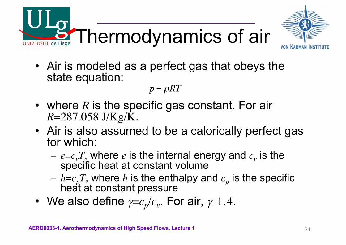
Thermodynamics of air• Air is modeled as a perfect gas that obeys the

state equation:

• where R is the specific gas constant. For air R=287.058 J/Kg/K.

• Air is also assumed to be a calorically perfect gas for which:– e=cvT, where e is the internal energy and cv is the

specific heat at constant volume– h=cpT, where h is the enthalpy and cp is the specific

heat at constant pressure• We also define g=cp/cv. For air, g=1.4.

24

p = ρRT


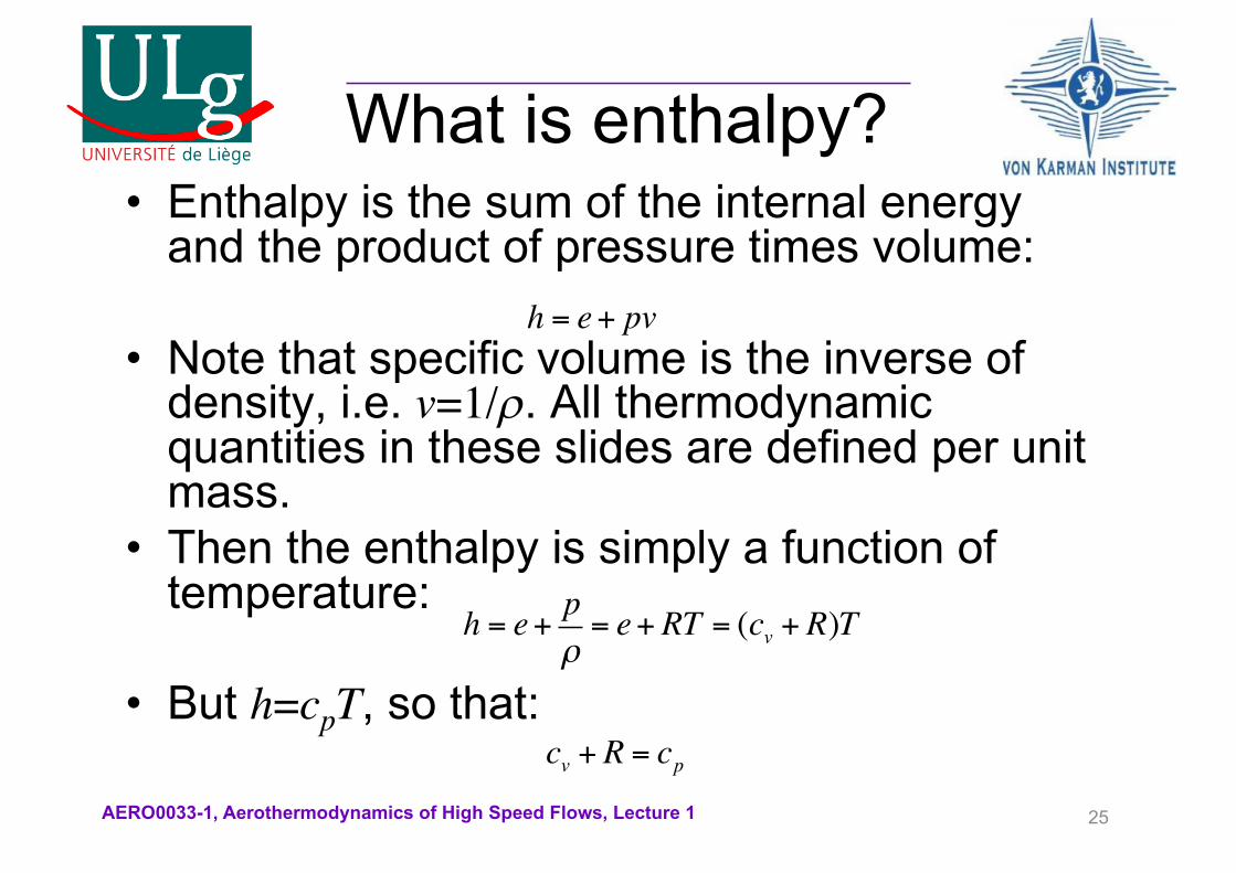
What is enthalpy?• Enthalpy is the sum of the internal energy

and the product of pressure times volume:

• Note that specific volume is the inverse of density, i.e. v=1/r. All thermodynamic quantities in these slides are defined per unit mass.

• Then the enthalpy is simply a function of temperature:

• But h=cpT, so that:

25

h = e+ pv

h = e+ pρ= e+ RT = (cv + R)T

cv + R = cp


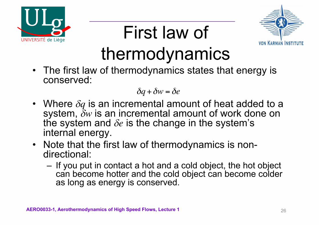
First law of thermodynamics

• The first law of thermodynamics states that energy is conserved:

• Where dq is an incremental amount of heat added to a system, dw is an incremental amount of work done on the system and de is the change in the system’s internal energy.

• Note that the first law of thermodynamics is non-directional:– If you put in contact a hot and a cold object, the hot object

can become hotter and the cold object can become colder as long as energy is conserved.

26

δq+δw = δe


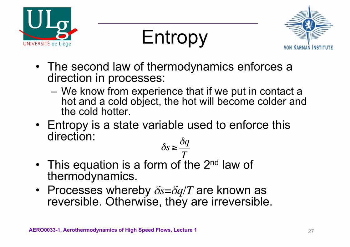
Entropy• The second law of thermodynamics enforces a

direction in processes:– We know from experience that if we put in contact a

hot and a cold object, the hot will become colder and the cold hotter.

• Entropy is a state variable used to enforce this direction:

• This equation is a form of the 2nd law of thermodynamics.

• Processes whereby ds=dq/T are known as reversible. Otherwise, they are irreversible.

27

δs ≥ δqT


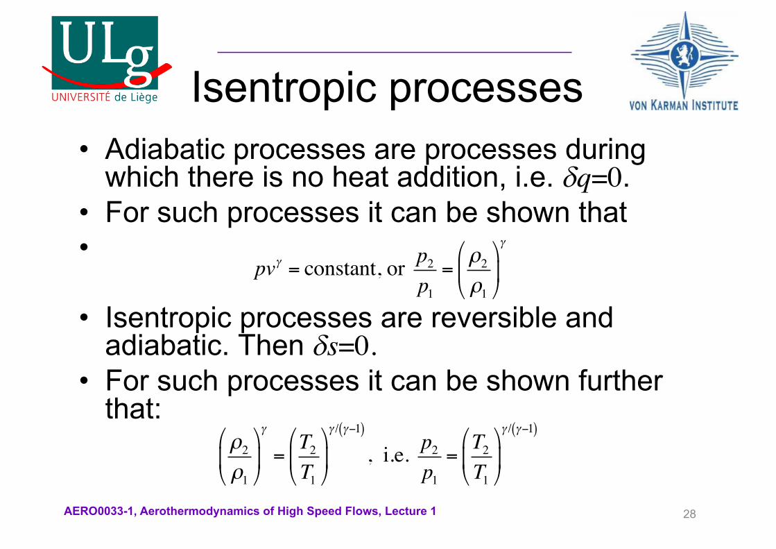
Isentropic processes• Adiabatic processes are processes during

which there is no heat addition, i.e. dq=0.• For such processes it can be shown that•

• Isentropic processes are reversible and adiabatic. Then ds=0.

• For such processes it can be shown further that:

28

ρ2

ρ1

!

"#

$

%&

γ

=T2

T1

!

"#

$

%&

γ / γ−1( )

, i.e. p2

p1

=T2

T1

!

"#

$

%&

γ / γ−1( )

pvγ = constant, or p2

p1

=ρ2

ρ1

!

"#

$

%&

γ


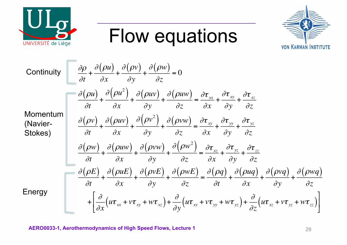
Flow equations

29

∂ρ∂t+∂ ρu( )∂x

+∂ ρv( )∂y

+∂ ρw( )∂z

= 0

∂ ρu( )∂t

+∂ ρu2( )∂x

+∂ ρuv( )∂y

+∂ ρuw( )∂z

=∂τ xx∂x

+∂τ xy∂y

+∂τ xz∂z

∂ ρv( )∂t

+∂ ρuv( )∂x

+∂ ρv2( )∂y

+∂ ρvw( )∂z

=∂τ xy∂x

+∂τ yy∂y

+∂τ yz∂z

∂ ρw( )∂t

+∂ ρuw( )∂x

+∂ ρvw( )∂y

+∂ ρw2( )∂z

=∂τ xz∂x

+∂τ yz∂y

+∂τ zz∂z

∂ ρE( )∂t

+∂ ρuE( )∂x

+∂ ρvE( )∂y

+∂ ρwE( )∂z

=∂ ρq( )∂t

+∂ ρuq( )∂x

+∂ ρvq( )∂y

+∂ ρwq( )∂z

+ ∂∂x

uτ xx + vτ xy +wτ xz( )+ ∂∂y

uτ xy + vτ yy +wτ yz( )+ ∂∂z

uτ xz + vτ yz +wτ zz( )!

"#

$

%&

Continuity

Momentum(Navier-Stokes)

Energy


Nomenclature• The lengths x, y, z are used to define

position with respect to a global frame of reference, while time is defined by t.

• u, v, w are the local airspeeds. They are functions of position and time.

• p, ρ, μ are the pressure, density and viscosity of the fluid and they are functions of position and time

• E is the total energy in the flow.• q is the external heat flux

30


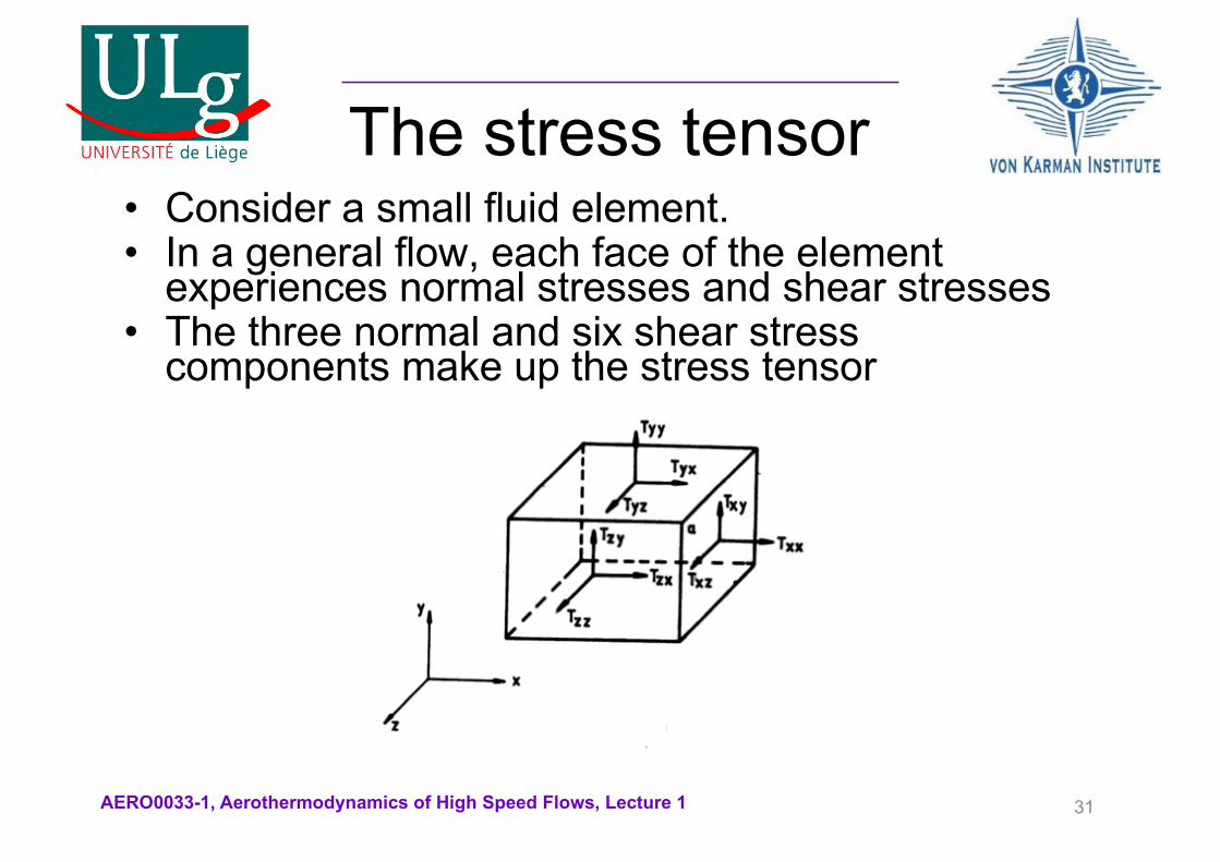
The stress tensor• Consider a small fluid element. • In a general flow, each face of the element

experiences normal stresses and shear stresses• The three normal and six shear stress

components make up the stress tensor

31


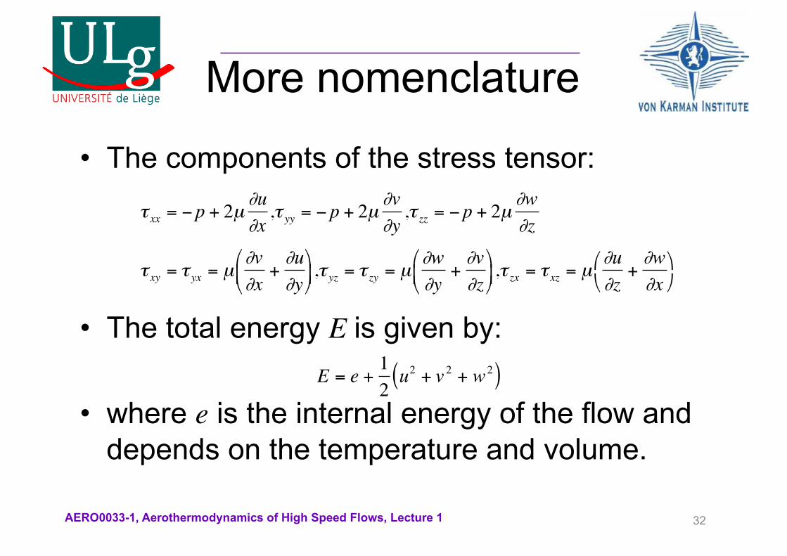
More nomenclature

• The components of the stress tensor:

• The total energy E is given by:

• where e is the internal energy of the flow and depends on the temperature and volume.

32

τ xx = −p + 2µ∂u∂x,τ yy = − p + 2µ ∂v

∂y,τ zz = −p + 2µ

∂w∂z

τ xy = τ yx = µ∂v∂x

+∂u∂y

% & '

( ) * ,τ yz = τ zy = µ

∂w∂y

+∂v∂z

% & '

( ) * ,τ zx = τ xz = µ

∂u∂z

+∂w∂x

% &

( )

E = e +12u2 + v 2 + w2( )

AERO0033-1, Aerothermodynamics of High Speed Flows, Lecture 1 33

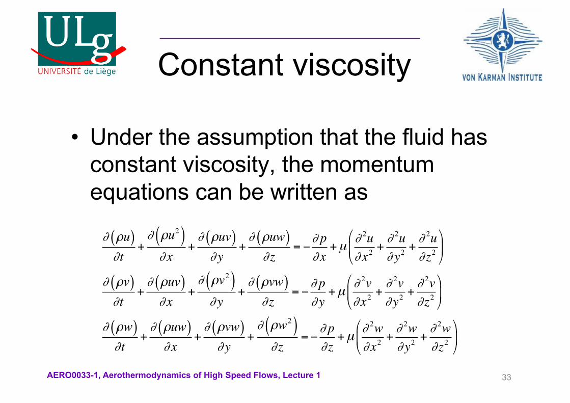
Constant viscosity

• Under the assumption that the fluid has constant viscosity, the momentum equations can be written as

∂ ρu( )∂t

+∂ ρu2( )∂x

+∂ ρuv( )∂y

+∂ ρuw( )∂z

= −∂ p∂x

+µ∂ 2u∂x2

+∂ 2u∂y2

+∂ 2u∂z2

"

#$

%

&'

∂ ρv( )∂t

+∂ ρuv( )∂x

+∂ ρv2( )∂y

+∂ ρvw( )∂z

= −∂ p∂y

+µ∂ 2v∂x2

+∂ 2v∂y2

+∂ 2v∂z2

"

#$

%

&'

∂ ρw( )∂t

+∂ ρuw( )∂x

+∂ ρvw( )∂y

+∂ ρw2( )∂z

= −∂ p∂z

+µ∂ 2w∂x2

+∂ 2w∂y2

+∂ 2w∂z2

"

#$

%

&'


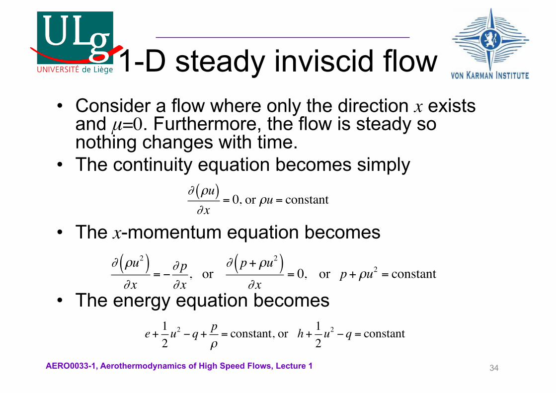
1-D steady inviscid flow• Consider a flow where only the direction x exists

and μ=0. Furthermore, the flow is steady so nothing changes with time.

• The continuity equation becomes simply

• The x-momentum equation becomes

• The energy equation becomes

34

∂ ρu( )∂x

= 0, or ρu = constant

∂ ρu2( )∂x

= −∂ p∂x

, or ∂ p+ ρu2( )

∂x= 0, or p+ ρu2 = constant

e+ 12u2 − q+ p

ρ= constant, or h+ 1

2u2 − q = constant


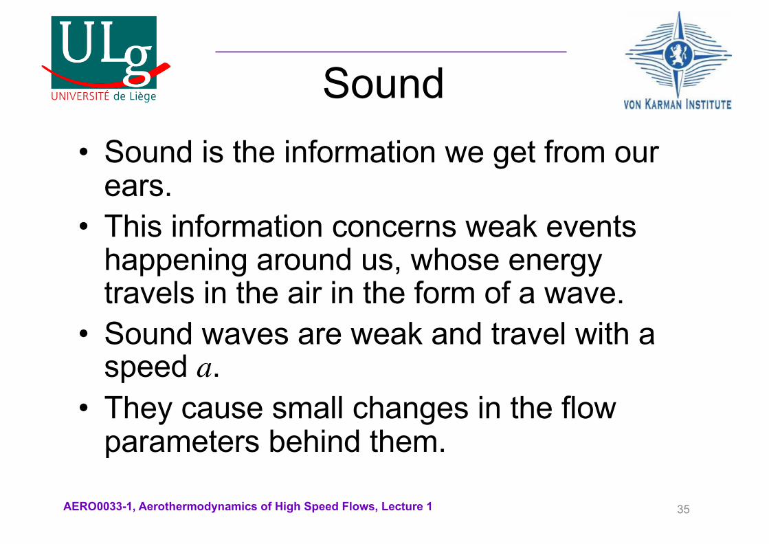
Sound• Sound is the information we get from our

ears.• This information concerns weak events

happening around us, whose energy travels in the air in the form of a wave.

• Sound waves are weak and travel with a speed a.

• They cause small changes in the flow parameters behind them.

35


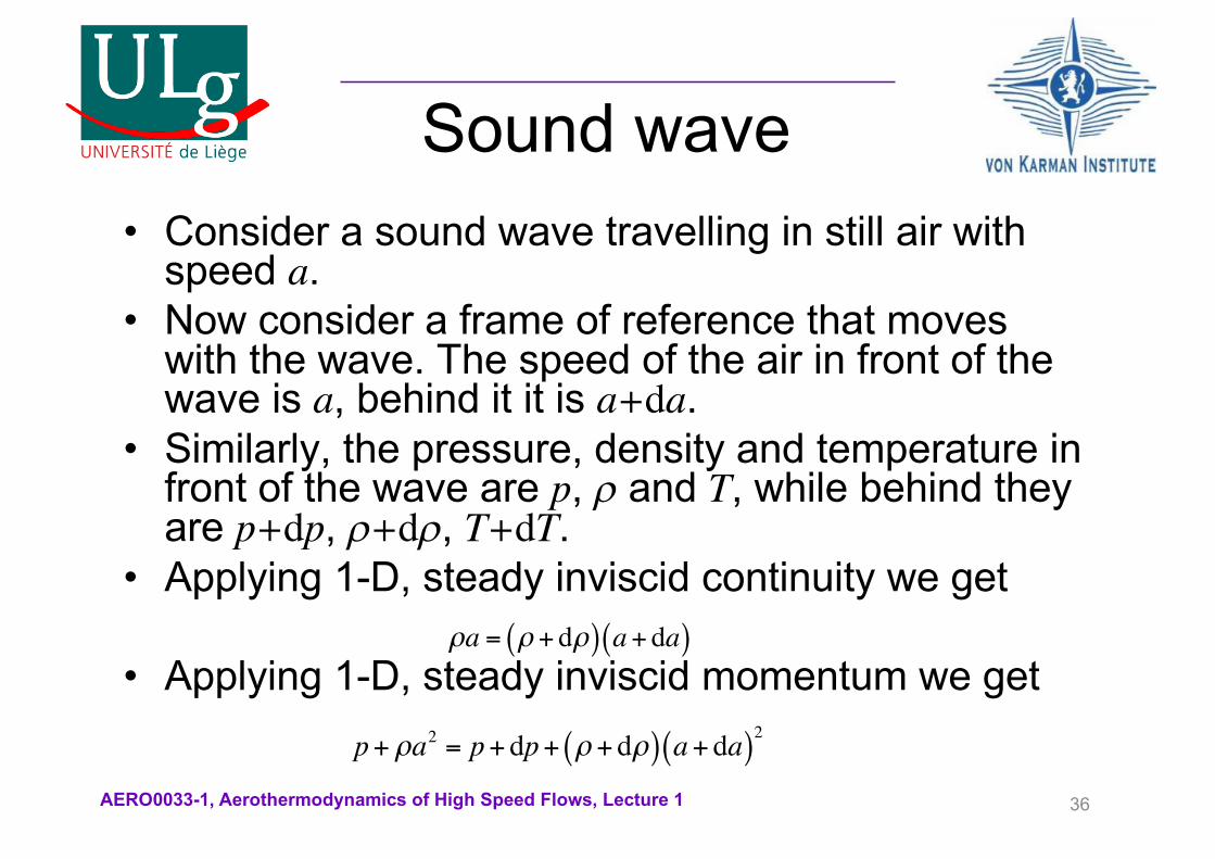
Sound wave• Consider a sound wave travelling in still air with

speed a.• Now consider a frame of reference that moves

with the wave. The speed of the air in front of the wave is a, behind it it is a+da.

• Similarly, the pressure, density and temperature in front of the wave are p, r and T, while behind they are p+dp, r+dr, T+dT.

• Applying 1-D, steady inviscid continuity we get

• Applying 1-D, steady inviscid momentum we get

36

ρa = ρ +dρ( ) a+da( )

p+ ρa2 = p+dp+ ρ +dρ( ) a+da( )2


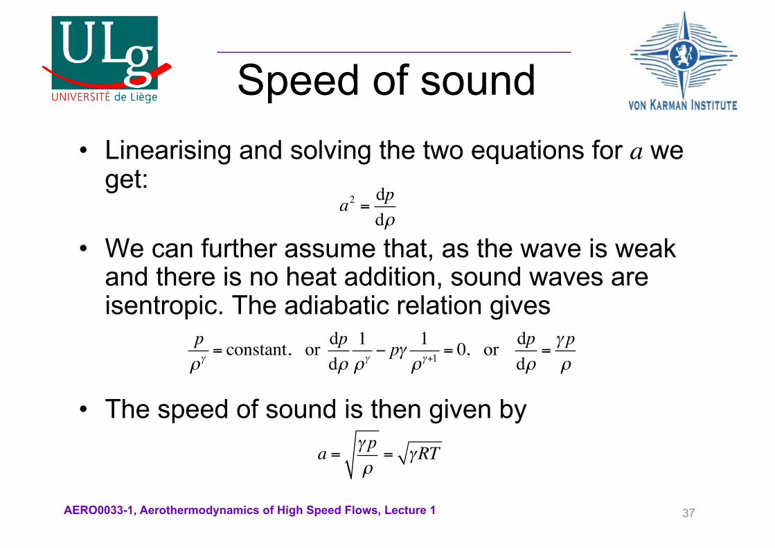
Speed of sound• Linearising and solving the two equations for a we

get:

• We can further assume that, as the wave is weak and there is no heat addition, sound waves are isentropic. The adiabatic relation gives

• The speed of sound is then given by

37

a2 = dpdρ

pργ

= constant, or dpdρ

1ργ

− pγ 1ργ+1 = 0, or dp

dρ=γ pρ

a = γ pρ= γRT


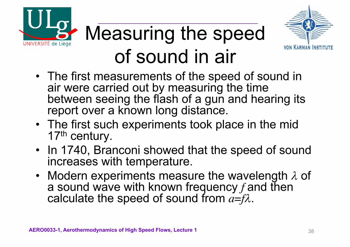
Measuring the speed of sound in air

• The first measurements of the speed of sound in air were carried out by measuring the time between seeing the flash of a gun and hearing its report over a known long distance.

• The first such experiments took place in the mid 17th century.

• In 1740, Branconi showed that the speed of sound increases with temperature.

• Modern experiments measure the wavelength l of a sound wave with known frequency f and then calculate the speed of sound from a=fl.

38


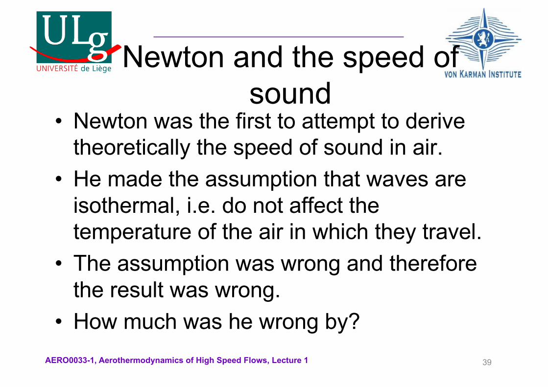
Newton and the speed of sound

• Newton was the first to attempt to derive theoretically the speed of sound in air.

• He made the assumption that waves are isothermal, i.e. do not affect the temperature of the air in which they travel.

• The assumption was wrong and therefore the result was wrong.

• How much was he wrong by?39


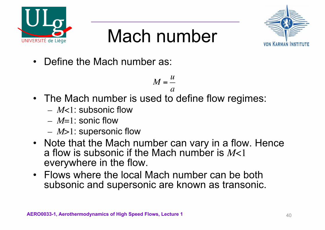
Mach number• Define the Mach number as:

• The Mach number is used to define flow regimes:– M<1: subsonic flow– M=1: sonic flow– M>1: supersonic flow

• Note that the Mach number can vary in a flow. Hence a flow is subsonic if the Mach number is M<1everywhere in the flow.

• Flows where the local Mach number can be both subsonic and supersonic are known as transonic.

40

M =ua


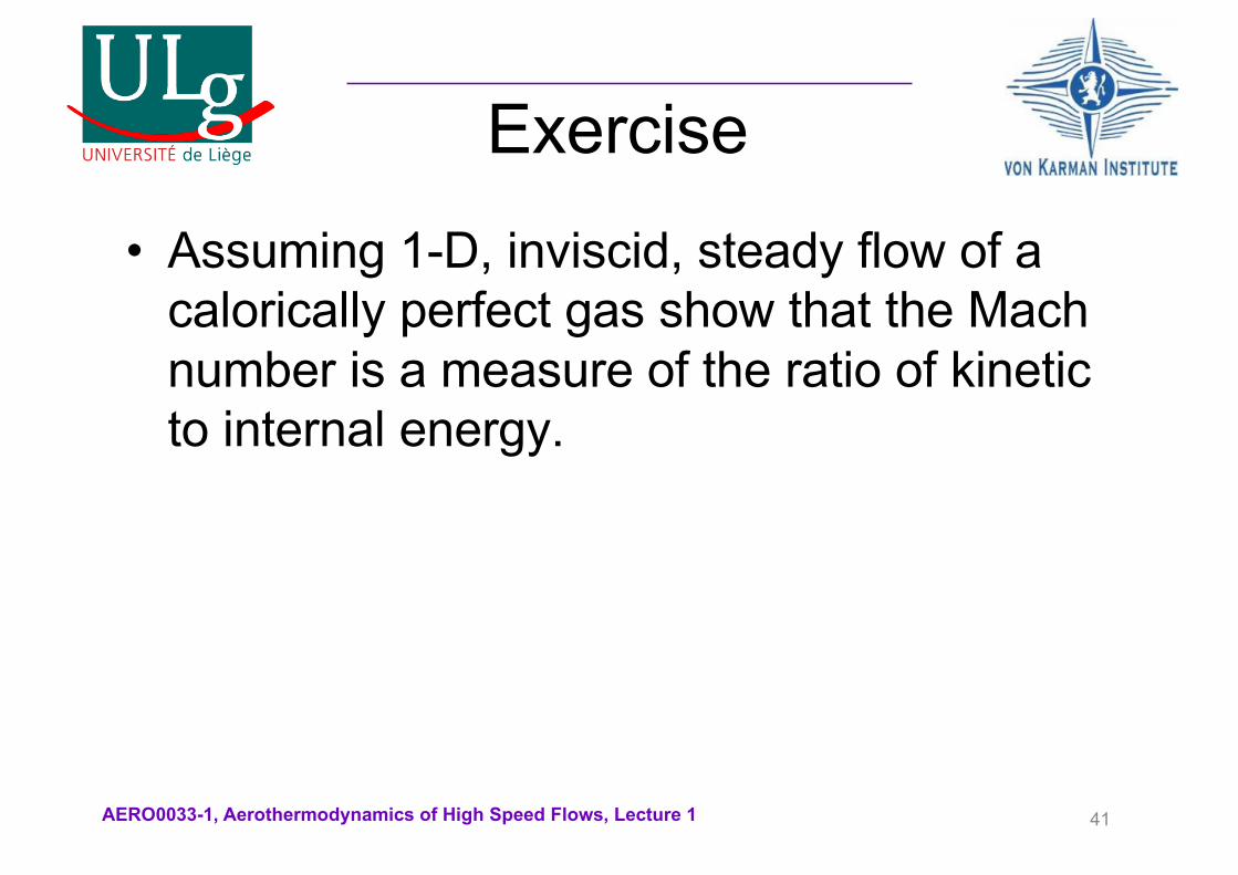
Exercise• Assuming 1-D, inviscid, steady flow of a

calorically perfect gas show that the Mach number is a measure of the ratio of kinetic to internal energy.

41


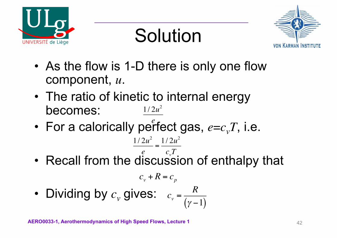
Solution• As the flow is 1-D there is only one flow

component, u. • The ratio of kinetic to internal energy

becomes:• For a calorically perfect gas, e=cvT, i.e.

• Recall from the discussion of enthalpy that

• Dividing by cv gives:

42

1/ 2u2

e

1/ 2u2

e=1/ 2u2

cvT

cv + R = cp

cv =Rγ −1( )


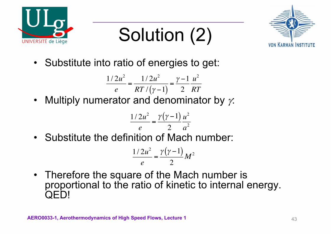
Solution (2)• Substitute into ratio of energies to get:

• Multiply numerator and denominator by g:

• Substitute the definition of Mach number:

• Therefore the square of the Mach number is proportional to the ratio of kinetic to internal energy. QED!

43

1/ 2u2

e=

1/ 2u2

RT / γ −1( )=γ −12

u2

RT

1/ 2u2

e=γ γ −1( )2

u2

a2

1/ 2u2

e=γ γ −1( )2

M 2


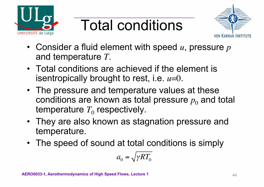
Total conditions• Consider a fluid element with speed u, pressure p

and temperature T.• Total conditions are achieved if the element is

isentropically brought to rest, i.e. u=0.• The pressure and temperature values at these

conditions are known as total pressure p0 and total temperature T0 respectively.

• They are also known as stagnation pressure and temperature.

• The speed of sound at total conditions is simply

44

a0 = γRT0


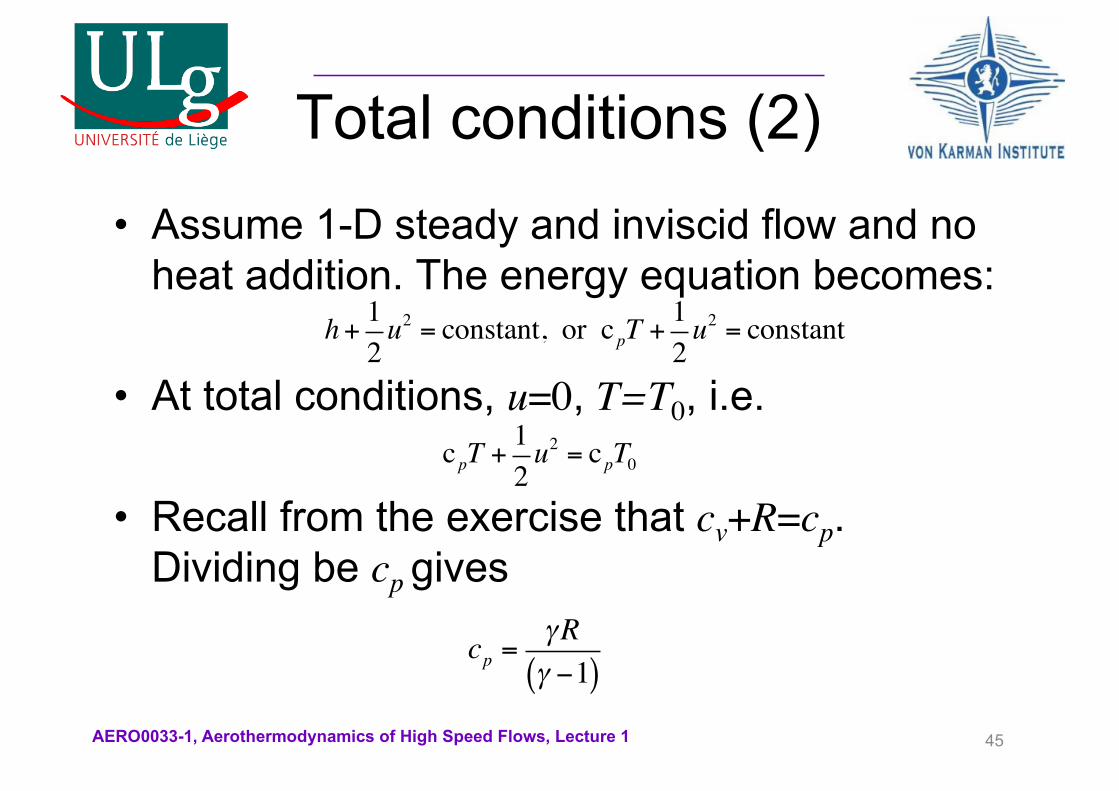
Total conditions (2)• Assume 1-D steady and inviscid flow and no

heat addition. The energy equation becomes:

• At total conditions, u=0, T=T0, i.e.

• Recall from the exercise that cv+R=cp. Dividing be cp gives

45

h+ 12u2 = constant, or c pT +

12u2 = constant

c pT +12u2 = c pT0

cp =γRγ −1( )


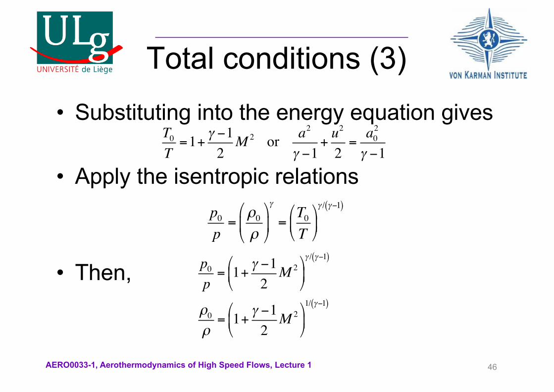
Total conditions (3)• Substituting into the energy equation gives

• Apply the isentropic relations

• Then,

46

T0

T=1+ γ −1

2M 2 or a

2

γ −1+u2

2=a0

2

γ −1

p0p=

ρ0ρ

!

"#

$

%&

γ

=T0T

!

"#

$

%&γ / γ−1( )

p0p= 1+ γ −1

2M 2"

#$

%

&'γ / γ−1( )

ρ0ρ= 1+ γ −1

2M 2"

#$

%

&'1/ γ−1( )


Sonic conditions• Consider a fluid element with speed u,

pressure p and temperature T.• Sonic conditions are achieved if the element

is adiabatically accelerated or decelerated until M=1.

• The pressure, temperature and speed of sound at these conditions are denoted by p*, T*, a*. The speed at sonic conditions is u=a*.

• The characteristic Mach number is defined as

47

M * =ua*


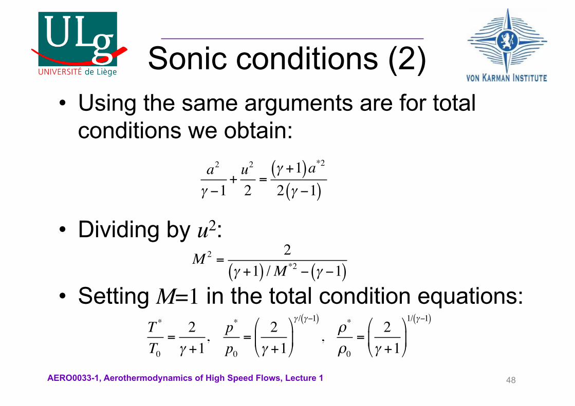
Sonic conditions (2)• Using the same arguments are for total

conditions we obtain:

• Dividing by u2:

• Setting M=1 in the total condition equations:

48

a2

γ −1+u2

2=γ +1( )a*2

2 γ −1( )

M 2 =2

γ +1( ) /M *2 − γ −1( )

T *

T0

=2

γ +1, p

*

p0

=2

γ +1!

"#

$

%&

γ / γ−1( )

, ρ*

ρ0

=2

γ +1!

"#

$

%&

1/ γ−1( )


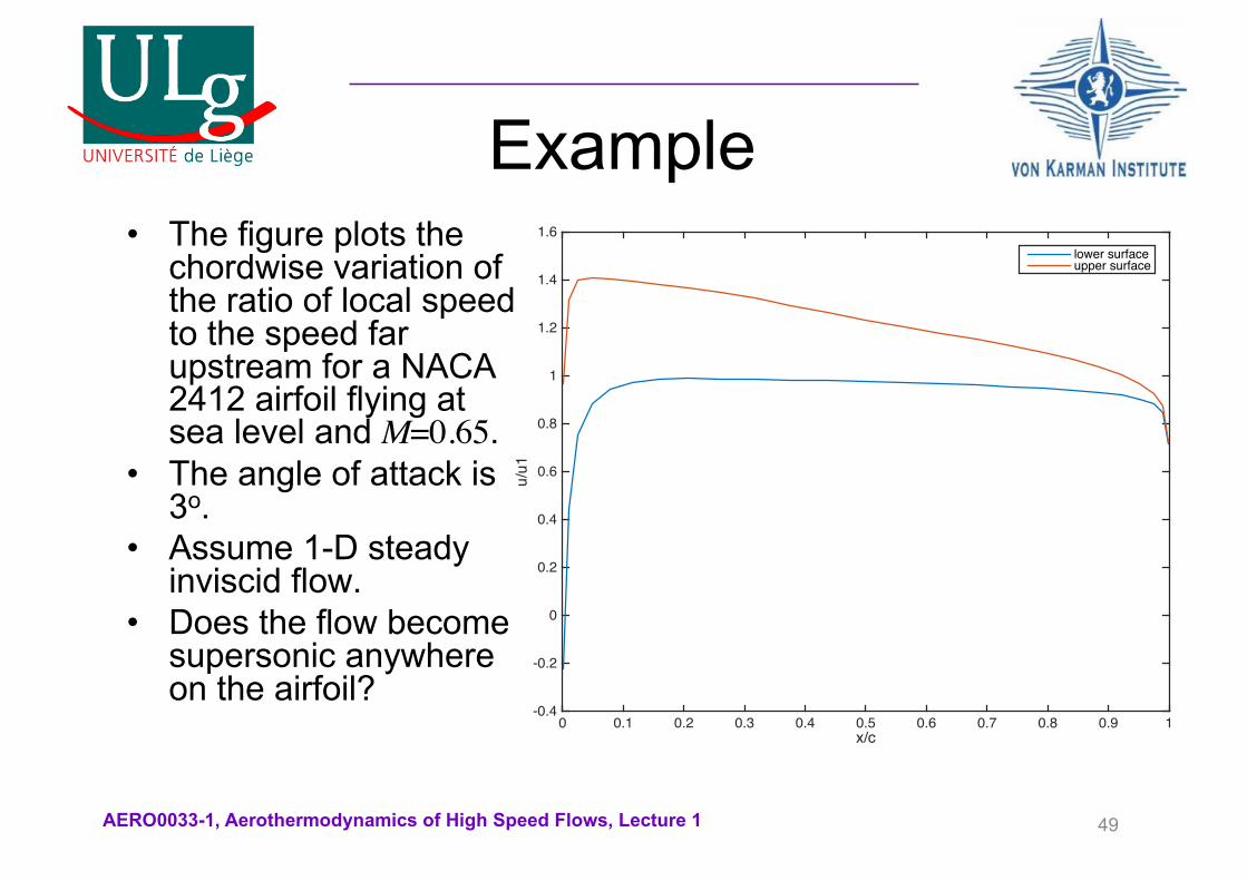
Example• The figure plots the

chordwise variation of the ratio of local speed to the speed far upstream for a NACA 2412 airfoil flying at sea level and M=0.65.

• The angle of attack is 3o.

• Assume 1-D steady inviscid flow.

• Does the flow become supersonic anywhere on the airfoil?

49

x/c0 0.1 0.2 0.3 0.4 0.5 0.6 0.7 0.8 0.9 1

u/u1

-0.4

-0.2

0

0.2

0.4

0.6

0.8

1

1.2

1.4

1.6lower surfaceupper surface


Answer• Far upstream the conditions are p1=101325

Pa, r1=1.225 kg/m3 and, using the state equation, T1=288.1 K.

• The speed of sound upstream is a1=340.3 m/s.• Combining the energy equation

• with• we get:

50

c pT +12u2 = constant

cp =γRγ −1( )

a2

γ −1( )+12u2 = constant


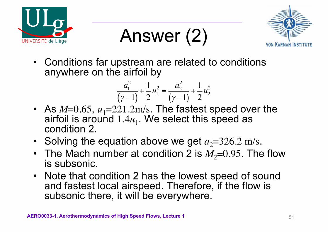
Answer (2)• Conditions far upstream are related to conditions

anywhere on the airfoil by

• As M=0.65, u1=221.2m/s. The fastest speed over the airfoil is around 1.4u1. We select this speed as condition 2.

• Solving the equation above we get a2=326.2 m/s.• The Mach number at condition 2 is M2=0.95. The flow

is subsonic.• Note that condition 2 has the lowest speed of sound

and fastest local airspeed. Therefore, if the flow is subsonic there, it will be everywhere.

51

a12

γ −1( )+12u12 =

a22

γ −1( )+12u22

Documents

Aerothermodynamics of High Speed Flows - uliege.be · AERO0033-1, Aerothermodynamics of High Speed Flows, Lecture 1 The sound barrier • Control reversal: Airfoil centreof pressure