A Pseudospectral Chebychev Method for the 2D …rosie/mypapers/renautfrojcp.pdfJOURNAL OF COMPUTATIONAL PHYSICS 124, 324–336 (1996) ARTICLE NO. 0063 A Pseudospectral Chebychev Method

JOURNAL OF COMPUTATIONAL PHYSICS 124, 324–336 (1996)ARTICLE NO. 0063

A Pseudospectral Chebychev Method for the 2D Wave Equationwith Domain Stretching and Absorbing Boundary Conditions

ROSEMARY RENAUT* AND JOCHEN FROHLICH†

*Department of Mathematics, Arizona State University, Tempe, Arizona 85287-1804 and †Konrad-Zuse-Zentrum fur Informationstechnik,Heilbronner Strasse 10, 10711 Berlin-Wilmersdorf, Germany

Received February 21, 1995

therefore the damping layer has to be large enough toprevent reentrant waves at the physical boundary. HenceIn this paper we develop a method for the simulation of wave

propagation on artificially bounded domains. The acoustic wave the approach is not only costly in terms of memory require-equation is solved at all points away from the boundaries by a ments but also it is not very flexible. In particular, thepseudospectral Chebychev method. Absorption at the boundaries appropriate damping layer must be determined for eachis obtained by applying one-way wave equations at the boundaries,

problem solved, dependent on location of the initial signalwithout the use of damping layers. The theoretical reflection coeffi-and the time interval over which a solution is required.cient for the method is compared to theoretical estimates of reflec-

tion coefficients for a Fourier model of the problem. These estimates The method proposed here, in which a one-way wave equa-are confirmed by numerical results. Modification of the method by tion is applied at the boundary, avoids these problems bya transformation of the grid to allow for better resolution at the removing both periodicity and damping layers. Moreover,center of the grid reduces the maximum eigenvalues of the differen-

the high-accuracy advantage of the pseudospectral spatialtial operator. Consequently, for stability the maximum timestep isapproximation is maintained by the use of a ChebychevO(1/N) as compared to O(1/N 2) for the standard Chebychev method.

Therefore, the Chebychev method can be implemented with effi- pseudospectral formulation. We note that the new tech-ciency comparable to that of the Fourier method. Moreover, numeri- nique is similar to a method proposed by Kopriva [3], forcal results presented demonstrate the superior performance of the the linearized gas dynamics equations, and by Carcionenew method. Q 1996 Academic Press, Inc.

[3] for the solution of the 2D wave equation recast as afirst-order linear hyperbolic system.

In Section 2 of the paper the absorbing boundary formu-1. INTRODUCTIONlation for the solution of the acoustic wave problem ispresented. The wave equation is solved at all points awayThis paper describes and evaluates a technique for the

application of artificial absorbing boundary conditions, in from the boundary by a Chebychev pseudospectralmethod, in which the spatial derivatives are approximatedconjunction with pseudospectral methods, for the simula-

tion of acoustic wave propagation. Typical numerical simu- via a Chebychev expansion of the solution. The absorbingboundaries are modelled by first-order one-way wavelations of wave propagation phenomena require a tech-

nique to eliminate spurious reflections from the numerical equations (OWWEs). The spatial derivatives of theseboundary equations are also approximated using the sameboundaries of the domain. Finite difference solutions

achieve this by the imposition of artificial boundary condi- Chebychev expansions. Integration in time is obtained byan implicit Crank–Nicholson method at the boundariestions which have been designed to absorb incident waves

at the boundary; see for example, [5, 7, 8, 10, 11, 19]. and a standard second-order discretization in time at theinterior points.Alternative approaches require the inclusion of a damping

region around the physical region, in which the solution The modified Chebychev method (see [16]) whichallows better resolution at the center of the grid, isis gradually damped to zero [4]. Kosloff and Kosloff [15]

have adapted this technique for the pseudospectral Fourier extended to second-order differential operators in space.Therefore, in Section 3, we also present graphs of themethod applied to forward modelling so that the acoustic

wave equation is modified by a damping term, non-zero eigenvalue distributions of the modified differentiationoperators. The spectral radii of these operators suggestonly in a damping region at the boundary. These methods

have been used for a wide variety of applications; see for that integration can proceed with timesteps O(1/N)instead of O(1/N 2). This is confirmed by numericalexample the recent papers by Kosloff et al. [17] and

Tessmer and Kosloff [22]. The solution, however, main- experiment.In Section 4 the theoretical reflection coefficient for thetains the periodicity induced by the Fourier method, and

3240021-9991/96 $18.00Copyright 1996 by Academic Press, Inc.All rights of reproduction in any form reserved.

ABSORBING BOUNDARIES FOR PSEUDOSPECTRAL METHODS 325

acoustic wave equation modified by OWWEs applied in quirement is achieved by the imposition of the appropriateone-way wave equations at the boundaries; see [5, 7, 8, 10,damping layers near the boundaries is compared with esti-

mates of the reflection coefficient for the modified equation 11, 19]. The lowest order one-way wave equation which iseffective is given bywith damping layer, presented in [15]. Note, that for nor-

mally incident waves, the reflection coefficient of the first-order OWWE is identically zero. Thus our comparisonsuggests a problem inherent in the pseudospectral Fourier S

t2 c

xD u(x, y, t) 5 0, (2.2)method but lacking in the Chebychev formulation: thedamping layer has to be very carefully designed with re-spect to its thickness and the shape of its damping function at the x 5 0 boundary. This equation allows for the com-in order to prevent both reflected and reentrant waves plete absorption of all waves incident normally to theover the time period of the simulation. boundary at x 5 0. For waves incident other than normally

We conclude with a performance evaluation of the the reflection coefficient is small for near-normal wavesChebychev pseudospectral method for acoustic wave simu- but increases to 1 for waves of glancing incidence at thelation in which the acoustic wave equation is solved at all boundary. The reflection can be reduced by applying eitherpoints, except those at the boundary, for which OWWEs higher-order one-way wave equations [19] or operators ofare used. The results are compared with the pseudospec- the kind (2.2) superposed to give absorption or some cho-tral Fourier formulation [14] applied, as in [15], to their sen set of incident waves [11]. In this paper we considermodified equation. Our results verify the superior perfor- (2.1) in conjunction with (2.2). The results presented dem-mance of the new method and confirm that the modified onstrate that (2.2) is effective in absorbing most outgo-Chebychev method can be implemented with a timestep ing waves.restriction O(1/N), equivalent to that used in the Fou- Equations of type (2.2) can be solved together with (2.1)rier method. in such a way that the appropriate OWWEs dominate near

The Chebychev formulation combined with the first- the boundary without modifying the solution on the innerorder OWWE offers a flexibility not found in the Fourier region. This formulation resembles the one considered inmethod. In particular, the absorbing boundary condition [15] and replaces the acoustic wave equation by the modi-need only be applied at one boundary, thus opening up fied equationthe possibility of the incorporation of absorbing boundariesinto problems with complicated geometries for which the

(1 2 («1 1 «2))(1 2 («3 1 «4))(utt 2 c2(uxx 1 uyy))need to do a domain decomposition eliminates the abilityto use periodic solution techniques. Furthermore, the

5 «1(ut 1 cux) 1 «2(ut 2 cux) (2.3)O(1/N) timestep restriction means that the overall cost is

1 «3(ut 1 cuy) 1 «4(ut 2 cuy).less than that for the Fourier method because the fastFourier transform (FFT) can still be applied for the calcula-tion of the derivatives and at the same time the numerical Here the functions «i are functions of x and y, chosen sodomains are reduced as compared to those employed in that the appropriate one-way wave equation dominates atthe Fourier method. each boundary. The width of the damping layer at a given

boundary then depends on the appropriate function «i . In2. THE METHOD the limit as the width of the damping layer goes to zero

the OWWEs are imposed only at the boundary. Precisely,2.1. OWWE and Spatial Discretization the modified equation (2.3) is then replaced by the system

of equations:The pseudospectral Chebychev method (see [2]) is em-ployed for the solution of the acoustic wave equation

utt 5 c2(uxx 1 uyy), t . 0, 0 , x , 1, 0 , y , 1(2.1)utt 5 c2(uxx 1 uyy),

ut 2 cux 5 0, x 5 0

ut 1 cux 5 0, x 5 1on the artificially bounded domain D 5 h(x, y) : 0 , x ,1, 0 , y , 1j. The solutions u 5 u(x, y, t) of (2.1) are

ut 2 cuy 5 0, y 5 0 (2.4)superpositions of plane waves which propagate in everydirection in two dimensions. Contributions which travel ut 1 cuy 5 0, y 5 1,towards the boundary of the domain D have to leave this

u(x, y, 0) given,domain freely, without reflection at the boundaries. Forthe solution of (2.1) by finite-difference methods this re- ut(x, y, 0) 5 0.

326 RENAUT AND FROHLICH

In this formulation the OWWEs are solved at the boundary Here u nij represents the discrete approximation to u(xi , yj ,

nDt), for a stepsize in time, Dt. The error in time is O(Dt 2)and the acoustic wave equation is used to update the solu-tion everywhere on the interior of the domain. which may be large compared to the high-order accuracy

in space of the pseudospectral spatial approximation. ButIn either formulation, (2.3) or (2.4), the approach of thepseudospectral method is to interpolate the function u(x, y, our numerical experiments show that the temporal error is

not a significant problem because the stability requirementt) along grid lines in both x and y directions. Derivatives ofu(x, y, t), with respect to x and y, are then approximated by limits Dt in relation to the grid sizes in the x- and y-direc-

tions by Dt 5 O(Dx 2min) and Dt 5 O(Dxmin), where Dxminthe derivatives of the interpolants. In our work we have used

both Chebychev and Legendre pseudospectral methods for is the minimum grid spacing for the Chebychev and modi-fied Chebychev methods, respectively.these spatial derivatives. Because no great advantage was

seen for the Legendre method our results emphasize the When the spatial derivatives in Eq. (2.5b) are approxi-mated by finite difference approximations the time deriva-Chebychev method which allows for implementation via a

fast Fourier transform; see Canuto et al. [2]. In either case, tives are typically approximated by an explicit method intime. Explicit methods can also be derived for the pseudo-after spatial discretization, (2.4) is replaced byspectral implementation; for example, for the boundarycondition at x 5 0, illustrative of all boundary conditions,(a) utt(xi , yj , t) 5 c2(Dxxu 1 Dyyu)(xi , yj , t),Euler’s method would take the explicit form

1 # i # N 2 1, 1 # j # M 2 1,

(2.5)u n11

0j 5 u n0j 1 cDt(Dxu)n

0j , (2.8)

(b) 5ut(0, yj , t) 5 c(Dxu)(0, yj , t), 0 # j # M

ut(1, yj , t) 5 2c(Dxu)(1, yj , t), 0 # j # M

ut(xi , 0, t) 5 c(Dyu)(xi , 0, t), 0 # i # N

ut(xi , 1, t) 5 2c(Dyu)(xi , 1, t), 0 # i # N.

which is only of first-order accuracy in time. On the otherhand, second-order accuracy in time is achievable with theexplicit midpoint, or Leapfrog, method,

u n110j 5 u n21

0j 1 2cDt(Dxu)n0j , (2.9)Here Dx , Dy , Dxx , Dyy , are first- and second-order differen-

tial operators in x and y, respectively [2] and (Du) (xi , yj ,t) denotes that the operator D is applied to u and evaluated But, a stability analysis immediately rules out (2.9) becauseat the grid point (xi , yj , t). The degrees of the interpolation the stability region of the midpoint method is just thein x and y are given by N and M, respectively. interval [21, 1] on the imaginary axis, which does not allow

for eigenvalues of the spatial operator to have any real2.2. Time Discretization part; see below. However, O(Dt 2) accuracy in time can

also be obtained by the implicit u-method,The choice of an appropriate time scheme for Eqs. (2.5a)and (2.5b) is not trivial. A first approach is to reformulatethe whole system (2.5) as a system of first-order differential u n11

0j 5 u n0j 1 cDt[u(Dxu)n11

0j 1 (1 2 u)(Dxu) n0j] . (2.10)

equations (ODEs) in time,

With u 5 As (2.10) is the Crank–Nicholson method. Theimplicitness does not present an implementation problemut 5 Au, where u 5 Sux

utD . (2.6)

if the interior values are updated via (2.7) before (2.10) isapplied. In this case, an implicit equation in terms of theboundary values is still obtained but can be solved directlyAs such it is amenable to solution by any appropriate ODEby taking advantage of the forms of (Dxu) n11

0j andsolver, which also includes the semi-implicit method of Tal(Dxu) n11

Nj , expressed as elements of a matrix vector product;Ezer and Kosloff [20]. But in [6], where the well-posednesssee the Appendix.of (2.6) is considered, Driscoll and Trefethen show that

A necessary, but not sufficient, requirement for the sta-the operator is highly nonnormal and therefore that thebility of a numerical implementation of an initial boundaryeigenvalues of the operator A are not well-conditioned.value problem is that both interior and boundary schemesConsequently, we chose not to use this ODE system. In-are individually stable [21]. The determination of this re-stead, in our experiments we adopted the standard second-quirement for pseudospectral approximations is not asorder differencing in time for Eq. (2.5a):straightforward as for finite difference methods. In particu-lar, the usual von Neumann analysis cannot be appliedu n11

ij 2 2u nij 1 u n21

ij 5 c2 Dt 2(Dxx 1 Dyy)u nij ,

(2.7) because it relies on a Fourier transformation to demon-strate the preservation of norms in the Fourier space and,1 # i # N 2 1, 1 # j # M 2 1.


hence, in the spatial domain. Therefore, for pseudospectral notation as in Kosloff and Tal Ezer [16], suppose that thecollocation points are found from the ‘‘stretching’’ of themethods, it is standard to use an eigenvalue approach to

stability. For this one considers the location of the eigenval- regular Chebychev collocation points:ues of the differential operator in relation to the stabilityregion of the ODE solver. However, this technique, called xi 5 g(zi , a), 21 # xi # 1, 0 # i # N, 0 # a # 1, (3.1)‘‘eigenvalue stability,’’ does not always give sufficient con-ditions for stability. Trefethen [23] discusses how well any andrequirements deduced from an analysis of the eigenvalueswill give reasonable estimates for Lax-stability. Moreover,

zi 5 2cos SifND, 0 # i # N.Reddy and Trefethen [18] show that for first-order opera-

tors the pseudospectra give more realistic stability restric-tions; see also [24]. For near-normal matrices, however,

Here a is a parameter of a ‘‘stretching’’ function g(z, a).the pseudospectra do closely approximate the eigenvaluesNote that transformation to the interval 0 # x # 1 is anand therefore an eigenvalue analysis is appropriate.additional trivial linear transformation. Differentiation ofIn the next section we present plots of the eigenvaluesa function f(x) is accomplished by making use of thefor the second-order differential operators. Weideman andchain rule,Trefethen [26] demonstrated that in this case these eigen-

values are not sensitive to the precision of the calculationand, hence, pseudospectra do closely approximate the ei- df

dx5

dzdx

dfdz

51

g9(z, a)dfdz

. (3.2)genvalues. Further, the eigenvalues are real and negativewith O(N 4) outliers. Therefore stability restrictions on the

Therefore for first-order differentiation the operator D istimestep are of order O(1/N 2), for explicit discretisationsreplaced by D 5 AD, where A is a diagonal matrix withof second-order time derivatives. For the boundary opera-entries Aii 5 1/g9(zi , a). Second-order differentiation istor the spectrum of the first-order operator is important.accomplished byThis operator, however, is far from normal and has eigen-

values in the left half plane, with O(N 2) outliers. It is forthis reason that we would not expect the midpoint method d 2f

dx2 5d

dx SdfdxD5

dzdx

ddz Sdf

dxD(3.3)

to be a viable method. Neither is Euler’s method a goodchoice because it has a stability region, just the circle in

51

g9(z, a) S 1g9(z, a)

d 2fdz2 2

g0(z, a)g9(z, a)2

dfdzD ,the left half plane with radius one and center at (21, 0),

which imposes very severe restrictions on the timestep inorder for the O(N 2) outliers of the first-order differential

and the second-order derivative operator D2 is replacedoperator to be moved within this circle. On the other hand,by D2 5 A2D2 1 BD, where A2 is the square of the diagonalthe Crank–Nicholson method is A-stable, with stabilitymatrix A, and B is the diagonal matrix with entries Bii 5region incorporating the whole left half plane. Thereforeg0(zi , a)/g9(zi , a)3.the O(N 2) outliers present no restrictions on the timestep

In Kosloff and Tal Ezer [16] plots are presented whichand our experiments use (2.10) with u 5 As.verify that the eigenvalues of the matrices D are insensitivewith respect to perturbations; in other words, the transfor-

3. THE MODIFIED CHEBYCHEV METHODmation actually serves to condition the spectra of the matri-ces D. The spectra of the matrices D2 are, however, muchOne disadvantage of the Chebychev pseudospectralbetter conditioned than those of D, even without stretch-method for the solution of equations (2.1) and (2.2) is theing; see Trefethen and Trummer [25]. In particular, theclustering of the grid points near the boundaries. This haseigenvalues of D2 are real, negative, and for interpolationthe effect of diminishing resolution at the center of theat the Chebychev extrema, as here, satisfygrid and also, in light of the earlier discussion, at the same

time, because of this clustering at the boundaries, imposingstricter limitations on the allowable timesteps for stable lim

NRysup

r(D2)N 4 # Ï11/4725 P 0.0482,

solutions. Kosloff and Tal Ezer [16] presented a modifiedChebychev method for the solution of problems with first-order spatial derivatives. Their approach is very easily ex- where r(D2) denotes the spectral radius of D2 . This O(N 4)

behaviour of D2 imposes a severe O(1/N 2) restriction ontended for application to second-order spatial derivatives,

´without additional work for the calculation of the deriva- the time step used in (2.7). In Fig. 1 we plot the eigenvaluesof D2 for various N and a 5 cos(jf/N), j 5 1, 2, 3, comparedtives, provided the appropriate coefficient matrices are set

up in an initialisation stage. Therefore, employing the same with the exact eigenvalues of the operator d 2/dx2, and


FIG. 1. (a)–(d) Eigenvalues of D2 and D2 , for N 5 16, 32, 64, and 128, respectively.

those of D2 . It can be seen that these eigenvalues are againreal and negative and that, dependent on a, respectivelyj, the spectrum more closely approximates that of d 2/dx2. TABLE IThese results are summarized in Table I. Furthermore,

Spectral Radius of the One-Dimensional Second-Orderevaluation of both the commutator of D2 and the conditionDerivative Operator D2of the matrix of normalised eigenvectors of D2 shows that

the matrices D2 are near normal. This is demonstrated in N j 5 1 j 5 2 j 5 3 UnmodifiedTable II.

16 5.0E 1 02 8.2E 1 02 1.3E 1 02 2.4E 1 03In our experiments we chose to use the function32 2.4E 1 03 4.5E 1 03 7.8E 1 03 4.4E 1 04g(z, a) 5 sin21(az)/sin21(a) suggested by Kosloff and Tal50 6.2E 1 03 1.2E 1 04 2.2E 1 04 2.7E 1 05Ezer [16], with a 5 cos(jf/N), j 5 1. Here j represents64 1.0E 1 04 2.1E 1 04 6.1E 1 04 7.5E 1 05

the number of waves, up to the maximum resolvable, which 128 4.4E 1 04 9.1E 1 04 1.7E 1 05 1.2E 1 07are not resolved by the grid. For j 5 1 maximal resolution,


TABLE II

Commutator C(D2) 5 iDT2 D2 2 D2 DT

2 i2/iDT2 D2i2 and Condition K(M) 5 iMi2iM 21i2 , of V and V, the Matrix of Normalized

Eigenvectors of D2 and D2 , Respectively

j 5 1 j 5 2 j 5 3 Unmodified

N C(D2) K(V) C(D2) K(V) C(D2) K(V) C(D2) K(V)

16 5.5E 2 02 1.20 1.1E 2 01 1.32 1.4E 2 01 1.41 1.6E 2 01 1.5732 5.5E 2 02 1.21 1.1E 2 01 1.34 1.4E 2 01 1.46 1.6E 2 01 1.8950 5.5E 2 02 1.21 1.1E 2 01 1.35 1.4E 2 01 1.49 1.6E 2 01 2.1364 5.5E 2 02 1.21 1.1E 2 01 1.35 1.4E 2 01 1.50 1.6E 2 01 2.28

128 5.5E 2 02 1.21 1.1E 2 01 1.36 1.4E 2 01 1.52 1.6E 2 01 2.74

rmax 5 N/2 2 1, is achieved, where rmax is the maximum 4. REFLECTION COEFFICIENTSwave number resolved by the grid. We note that this choice

In Kosloff and Kosloff [15] a derivation of the reflectionof a is not necessarily the best choice in terms of accuracycoefficient for the modified acoustic wave equationbecause of the trade-off between accuracy and resolution

in space. But, because of stability, it does allow integrationin time with a timestep which is significantly larger than 2p

dt 2 5 c2 2pdx 2 2 2c

dpt

2 c2p (4.1)that allowed by the Chebychev method, in fact for N 5128 a timestep some 16 times larger can be employed; seeTable III. In cases where physically the time evolution on

is presented. c is a damping function which is non-zerothe small scale is not required this can lead to an enormousonly at a set of grid points within a predetermined distancereduction in computational effort. Moreover, we see fromof the boundary and is defined by, as used in [15],the analysis in [16], that as we improve spectral accuracy

by increasing j, and consequently decreasing a, the time-step must decrease to maintain stability, and hence the

c 5U0

cosh(n ? n)2 , (4.2)temporal accuracy also improves. An issue in simulationsof wave propagation phenomena is the lack of resolutionat the center of the grid and, hence, this symmetric transfor-mation, with a near to 1, is the appropriate choice. For where n is the number of grid points of the grid point

xi from the closest boundary. The parameters U0 and nmodels with different boundary conditions at oppositeboundaries it may be appropriate to adopt the unsymmetric determine the width of the boundary layer and how sharply

c tends to zero at the physical boundary. In our two-transformation of Kosloff and Tal Ezer [16]. The transfor-mations suggested by Bayliss and Turkel [1] could also dimensional experiments we mapped the physical domain

onto the domain [0, 1] 3 [0, 1], so that the computationprovide reasonable alternatives. In these cases the stabilityanalysis has to be repeated, but the techniques are the was performed on a domain [2D, 1, 1 D] 3 [2D, 1 1 D],

with the same damping function used at all boundaries.same.

TABLE III

Observed Stability Limits on cDt for Two-Dimensional Problem

j 5 1 j 5 2 j 5 3

N cDt a cDt a cDt a Unmodified

16 3.1E 2 02 .9781 2.4E 2 02 .9135 1.9E 2 02 .9425 1.4E 2 0232 1.4E 2 02 .9949 1.0E 2 02 .9795 8.0E 2 03 .9541 3.3E 2 0350 9.0E 2 03 .9979 6.4E 2 03 .9918 4.7E 2 03 .9816 1.3E 2 0364 6.9E 2 03 .9988 4.8E 2 04 .9950 3.6E 2 03 .9888 8.1E 2 04

128 3.3E 2 03 .9997 2.3E 2 04 .9988 1.7E 2 03 .9972 2.0E 2 04


results are provided to support these experiments. In par-ticular, in [15] a grid with N 5 64 and a damping layerover 15 grid points were used. There, the damping layerwas obtained by choosing n 5 0.18 with U0 5 40 in (4.2).But, in order to have a damping layer over 15 grid pointswith this choice of c, there is a discontinuity in c at thedamping layer boundary, c(0) 5 c(1) > 12.8, uc(x)u 5 0,x [ (0, 1). This is a compromise chosen in [15] to fulfillthe following contradictory requirements: For fixed widthof the layer transition is small if the integral of c is largeand if the gradient of c is small the reflection is small.However, if c has to increase from zero at the edge of thelayer to a significant value and go back to zero at the otheredge there has to be some gradient and, hence, reflection.The difficult task is now to find a shape that meets bothrequirements. The problem of the damping layer approachresides in the fact that this can not, by construction, becompletely achieved, even in the 1D case. In order toFIG. 2. Comparison of damping layer functions.illustrate what happens when c is chosen in a wrong waywe report numerical computations when n 5 3.6 and n 50.18, for U0 5 40 but in the latter case the damping layerFor the one-dimensional analysis of the reflection coeffi-

cient we make the equivalent assumptions for the solution is not restricted to 15 grid points. The correspondingreflection and transmission coefficients are depicted inof (4.1).

The reflection coefficient for a plane sinusoidal wave Fig. 2 and compared with the choice in [15]. Observethat with the latter choice transmission can be successfullye2ikxeigt incident from the left on the physical boundary at

x 5 1 can be calculated using the propagator matrix method suppressed but at the price of admitting some reflection,in particular for small wavenumbers. For the extremeof Haskell [9]. The application of this method to the deter-

mination of the reflection coefficient is well-described in choice n 5 3.6 the transmission is unacceptably high. Thenumerical calculations confirm these theoretical predic-[15] and only necessary ideas are given here.

The idea of the propagator method is to divide the region tions.We conclude from this analysis that damping layers, asin which c is nonzero, 1 # x # 1 1 D, into small intervals

on each of which c is taken to be constant. Within each a means for absorbing waves at artificial boundaries, mustbe used with caution in the Fourier method. With a carefulinterval there is both a left- and a right-travelling wave,

each of different amplitude, which are propagated ac- choice of the damping function the resulting reflection andtransmission may be negligible. But our numerical resultscording to the underlying partial differential equation. Sup-

pose that a wave of unit amplitude is incident at x 5 1. have shown cases in which reflection or transmission tothe opposite boundary may be significant, particularly ifIdeally the reflected left-travelling wave has an amplitude

R P 0. In practice, R is determined via the solution of the initial signal is close enough to the damping layerboundary. This has severe consequences in terms of mem-successive transmission–reflection problems on each sub-

interval, which, in turn, by periodicity, depend on the am- ory requirements, in particular, for three-dimensionalproblems.plitudes of the left- and right-travelling waves at x 5 0, at

which it is assumed the left travelling wave has amplitude On the contrary, however, the Chebyshev-pseudospec-tral method can be successfully applied without the compu-zero. But the right travelling wave is transmitted back into

the interior domain with an amplitude, T, hopefully near tational and memory overhead of a damping layer if a first-order absorbing boundary condition is used at the artificialzero. Hence, ideally, not only should we have R P 0 but

also T P 0, so that no reentrant waves are noticeable at boundary. Because the Chebychev method can also beimplemented with the use of fast Fourier transforms itsthe opposite boundary. Furthermore, the effects of the

boundary layer should not extend into the interior, so that implementation does not require a significant increase incost as compared to the Fourier-pseudospectral method.the function c should be negligible on the interior.

In Fig. 2 we present calculations of the reflection and Consequently, the non-periodic discretisation without thedamping layer presents a much more efficient and robusttransmission coefficients, R and T, respectively, for differ-

ent choices of c. Our numerical experiments in Section 5 method for the solution of wave propagation problems. Inthe next section our numerical results verify these conclu-have been designed to permit a comparison with the work

of Kosloff and Kosloff [15], and therefore the theoretical sions.


5. NUMERICAL RESULTS Note that for the Fourier method applied to a physicalinterval [xL , xR] periodicity means that numerically gridpoints are on the interval [xL , xR 2 Dx]. In contrast, forFirst we give an overview of the numerical tests which

have been carried out. Acoustic wave propagation can be a Chebychev grid the whole physical interval is used.Therefore, the Fourier 64 3 64 grid actually corresponds,modelled by the periodic Fourier pseudospectral solution

of the modified acoustic wave equation (4.1), where c is by periodicity, to a 65 3 65 grid, and, with a dampinglayer of effective width 15 grid points, is equivalent to agiven by (4.2). This is the method of [15] and has been

implemented as a reference. But the model given by (4.1) Chebychev grid 50 3 50. The effective grid on the physicalregion is then 50 3 50 in both cases. The acoustic velocityis not limited to a periodic formulation and we have also

solved it using a Chebychev pseudospectral implementa- was taken as 2, in dimensionless units, equivalent to the2000 ms21 used in [15]. Simulations with an internal layertion. This implementation, however, does not succeed in

removing the entire energy of the incident wave at the of reduced sound velocity, equivalent to the embeddedvelocity layer simulations in [15], were also carried out,boundary, because even in the one-dimensional case there

is still a certain amount of reflection at the physical bound- using a local dimensionless acoustic velocity of 1.2. Thedamping layer was also set up using Eq. (4.2) as indicatedary. Furthermore, it requires additional cost due to the

presence of the damping layer. For these two reasons this in Section 4. To give an effective damping layer over 15grid points the parameters U0 5 40 and n 5 0.18 wereChebychev implementation is outperformed by the Cheby-

chev implementations described below. chosen, but, as indicated in Section 4, with the discontinuityin c at the internal damping layer boundary.Before continuing with non-periodic formulations we

also observe that a Fourier pseudospectral implementation For both the Fourier and scaled Chebychev methods adimensionless timestep Dt 5 0.0045, near the stability limitof the modified equation (2.3) would also be possible. Re-

gardless of the appearance of discontinuities in the coeffi- for both methods, was used. To maintain stability of theunscaled Chebychev method the timestep was reduced tocients, this does not make sense, however. The construction

of (2.3) aims at achieving zero reflection and, at the same 0.0006. Measurements were made at equivalent dimen-sionless times in all cases.time, full transmission at these boundaries. Due to the

wraparound effect of the periodic formulation the solution The simulations were initiated with pulses of the formwould be subject to the same deleterious transmission ofwaves through opposite boundaries, as argued in the previ- u(x, y, 0) 5 e2r2a,ous section.

The solution of (2.3) with a non-zero thickness OWWE where r2 5 (x 2 x0)2 1 (y 2 y0)2 for an initial pulse centeredat (x0 , y0). For Figs. 4 and 7 the pulse was initiated at thedamping layer by a pseudospectral Chebychev discretisa-

tion does, however, lead to satisfactory results. Our compu- center of the domain, (x0 , y0) 5 (0.5, 0.5), and for Fig. 5the pulse was moved nearer the corner, (x0 , y0) 5 (0.1,tations show that this still remains true in the limit where

this layer goes to zero and the OWWEs are imposed only 0.1). In all cases, the weighting in the pulse was taken tobe a 5 500. Other choices give qualitatively similar results,at the boundary points, leading to (2.5). Furthermore, the

latter computations are more efficient, requiring not only but require longer time simulations on larger domains toelucidate the results.a less dense grid but also allowing a direct implementation

of the implicit Crank–Nicholson discretisation of the The results are illustrated in Fig. 3–7. In Figs. 3a and3b we present a comparison of the performance of theboundary operators. Therefore, this is the approach which

has been retained and for which results are given here. Fourier method with the different c functions, by plottingthe evolution of the pulse on the domain as measured byLegendre pseudospectral discretisations can also be

used, but they give very similar results to the Chebychev the L2 norm over the physical part of the grid. Here thethree choices of c discussed in Section 4 are used. Namely,series. In particular, the stability results are much the same,

exhibiting again critical timesteps of O(1/N 2)). The modi- (i) n 5 0.18, U0 5 40 with the discontinuity in c at thedamping layer boundary, (ii) n 5 0.18, U0 5 40, but withfied Chebychev discretisation described in Section 3 over-

comes this restriction and leads to the third set of results the function c going continuously to zero away from thedamping layer, and (iii) n 5 3.6, U0 5 40. For Fig. 3a adescribed in the following paragraphs.

In order to allow comparison between the Fourier and pulse is initiated at the center of the domain and in Fig.3b it is initiated at the corner. The effect of c ? 0 on theChebychev pseudospectral methods the physical region

was always taken as [0, 1] 3 [0, 1] and in all cases it is interior is, as expected, that the pulse is overdamped onthe interior domain. On the other hand, the high transmis-only this physical region which is plotted. To also allow

comparison with the results presented by Kosloff and Kos- sion of the n 5 3.6 case is also verified. Although thediscontinuous choice for c does give the better results andloff [15], calculations with the Fourier method were done

for a 64 3 64 grid, and a damping layer of 15 grid points. is used in the comparisons with the Chebychev methods,


FIG. 3. Comparisons of ‘‘energy’’ for a pulse initiated (a) at the center and (b) at the corner, respectively.

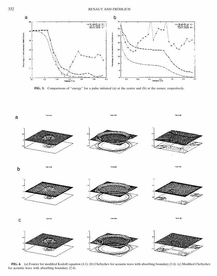
FIG. 4. (a) Fourier for modified Kosloff equation (4.1). (b) Chebychev for acoustic wave with absorbing boundary (2.4). (c) Modified Chebychevfor acoustic wave with absorbing boundary (2.4).


we also see that the discontinuity does give rise to greater the Chebychev implementations, i.e., high accuracy butresolution restricted in the center of the grid for Cheby-reflection than is desirable.

Figure 4 shows the evolution of a pulse placed in the chev, as compared to the modified Chebychev, j 5 1, withhigh resolution but reduced accuracy.center of the grid until it has propagated out of the physical

region, with a constant velocity of 2.0. The performance To allow comparison of these simulations we also plotin Fig. 6, as in Fig. 3, the L2 measure of how the pulseof all three methods is apparent, with in all cases some

residual reflection evident. This is most easily observed by evolves on the domain. From Fig. 6a we see that the Fourierand Chebychev methods perform nearly identically untilexamining the contour plots associated with each result.

In particular it can be seen in all cases that there are the pulse leaves the physical region and the greater reflec-tion of the Fourier method is evident. For simulations oversignificant corner effects where reflection at two bound-

aries meeting in a corner causes superposition of the two longer time periods the Chebychev methods continue toshow negligible energy but the Fourier energy oscillatesreflections and hence the increased reflection observed in

the contours emanating from the corners. In finite-differ- over time until the wave is eventually completely attenu-ated over the damping layer. Figure 6b very clearly showsence methods these effects are alleviated by the use of

special corner conditions applied at the corner and for a that the discontinuity in c(x) at the physical boundaryleads to a reflection of the pulse when it is initiated veryfew points near the corner. The same adjustments could

also be considered in this case. Figures 4b, 5b, and Figures close to the physical boundary. We have seen that this canbe reduced by taking a much wider damping layer, so that4c, 5c show a comparison between the two extremes of



FIG. 6. Comparisons of ‘‘energy’’ for a pulse initiated (a) at the center and (b) at the corner, respectively.

the discontinuity in c(x) is eliminated and the resulting L2 four grid points in the Fourier discretisation. Note that thediscontinuity in sound velocity can easily be accounted forcurve follows that of the Chebychev simulations.

We conclude with a test problem more oriented towards in the OWWE by modifying the value of c in (2.4). Figure7 shows a comparison of the solutions obtained with theapplications, the embedded velocity layer discussed in [15].

The layer of lower sound velocity is oriented parallel to three methods discussed. We observe that despite the jumpin the coefficient the pseudospectral methods behave quitethe y-axis (directed away from the spectator in perspective

views) and situated just right of center, having a width of well for this problem. The results also demonstrate that the



present OWWE-formulation for the absorbing boundary is ut

2 c1ux

5 0 at x 5 0

(A1)still successful.

Stability limits on cDt for all these two-dimensional simu-lations are given in Table III and verify that the modified u

t1 c2

ux

5 0 at x 5 1.method can proceed with timesteps of the same size asthose used for standard Fourier pseudospectral simula-tions. Here c1 and c2 represent the wave propagation speeds at

the left and right boundaries, respectively. For simplicity,in the derivation of the scheme, we assume u 5 As. Extension

6. CONCLUSIONS to arbitrary u is immediate. At the left boundary, x 5 0,the Crank–Nicholson scheme corresponds toA method for the simulation of wave propagation on

an artificially bounded domain has been described. Theapproach is novel in that commonly used OWWEs are u n11

0 5 u n0 1 c1

Dt2

[(Du)n110 1 (Du)n

0], (A2)incorporated in a non-periodic pseudospectral solution ofthe acoustic wave equation formulated as a second-orderPDE. As such, the formulation allows the high spatial where (Du)n

0 5 oNj50 d0j u n

j and D is the matrix of the first-accuracy of pseudospectral methods which leads to negligi- order differential operator d/dx, with entries dij . Becauseble numerical dissipation and makes this type of method we assume that the values of u n

ij are updated at the interiorparticularly interesting for the computation of wave propa- grid points prior to update of the boundaries, Eq. (A2) isgation phenomena. Compared to periodic Fourier dis- implicit in u n11

N and u n110 only:

cretisations the non-periodic approach first of all allowszero normal reflection at the boundary, a topic we havediscussed in detail. Second, it can be used with similarly (Du)n11

0 5 d00u n110 1 d0Nu n11

N 1 ON21

j51d0j u n11

j .sized time steps when employing a ‘‘stretching’’ transfor-mation of the Chebychev points. Finally, these kinds ofmethods exhiit flexibility with respect to the particular Therefore, with k1 5 c1Dt/2,conditions which can be imposed on the boundary anddomain decomposition. The discretization in space and

(1 2 k1 d00)u n110 2 k1d0N u n11

N 5 b n0 , (A3)time of the Chebychev implementation has been fully ad-

dressed. Of particular note is that we have also demon-strated the high spectral accuracy of the spatial transforma- where bn

0 5 un0 1 k1 [oN21

j51 d0jun11j 1 (Du)n

0] is known.tion for second derivative operators. Equivalently, the equation at the right-hand boundary is

Future directions of this research are immediately sug-gested by the following observations. Because the bound-

k2 dN0 u n110 1 (1 1 k2 dNN)u n11

N 5 b nN

(A4)ary conditions are implemented directly by the solution5 u n

N 2 k2 [oN21j51 dNj u n11

j 1 (Du)nN],of given boundary equations, not only is the technique

obviously extendable to three dimensions, but also it isnot necessary that all boundaries use the same boundary where k2 5 c2D t/2. Equations (A3) and (A4) represent aconditions. A particularly interesting option would be the set of two linear equations in two unknowns, u n11

0 , u n11N ,

simulation of surface waves at the surface boundary. Fur-thermore, improved absorption at an absorbing boundarycan be achieved by the implementation of higher-order A Su n11

0

u n11ND5 Sb n

0

b nND5 bn,

OWWEs. Moreover, because the boundary operator isone-dimensional, the OWWEs can also be used for mediawith heterogeneities parallel to the boundary, but constant whereperpendicular to the boundary. This has been aptly demon-strated for finite difference models by Higdon [12].

A 5 S1 2 k1 d00 2k1 d0N

k2 dN0 1 2 k2 dNND.

APPENDIX: IMPLEMENTATION OF THECRANK–NICHOLSON METHOD AT THE BOUNDARY

For both the Chebychev and the modified Chebychev pseu-dospectral methods the entries of the differential operatorSuppose that absorbing boundary conditions are applied

at both the x 5 0 and x 5 1 boundaries: D are such that d00 5 dNN and d0N 5 2dN0 , see [2, p.


4. C. Cerjan, D. Kosloff, R. Kosloff, and M. Reshef, Geophysics 50,69]. Therefore,705 (1985).

5. R. Clayton and B. Engquist, Bull. Seismol. Soc. Am. 67, 1524 (1977).6. T. A. Driscoll and L. N. Trefethen, Cornell University, 1993 (unpub-A 5 S1 1 k1 dNN k1 dN0

k2 dN0 1 1 k2 dNND lished).

7. B. Engquist and A. Majda, Comm. Pure Appl. Math. 32, 313 (1979).8. L. Halpern and L. N. Trefethen, J. Accoust. Soc. Am. 84, 1397 (1988).

and it immediately follows that9. N. A. Haskall, Bull. Seismol. Soc. Am. 43, 17 (1953).

10. R. L. Higdon, Math. Comput. 47, 437 (1986).11. R. L. Higdon, Math. Comput. 49, 65 (1987).u n11

0 51

uAu((1 1 k2 dNN)b n

0 2 k1 dN0 b nN),

12. R. L. Higdon, J. Comput. Phys. 101, 386 (1992).13. D. A. Kopriva, FSU-SCR1-92C-17, Florida State University, 1992

(unpublished).u n11N 5

1uAu

(2 k2 dN0 b n0 1 (1 1 k1 dNN)b n

N),14. D. D. Kosloff and E. Baysall, Geophysics 47, 1402 (1982).15. R. Kosloff and D. Kosloff, J. Comput. Phys. 63, 363 (1986).16. D. Kosloff and H. Tal Ezer, J. Comput. Phys. 104, 457 (1993).where uAu represents the determinant of A.17. D. Kosloff, D. Kessler, A. Q. Filho, E. Tessmer, A. Behle, and R.

Strahilevitz, Geophysics 55(6), 734 (1990).ACKNOWLEDGMENTS 18. S. C. Reddy and L. N. Trefethen, Comput. Methods Appl. Mech.

Eng. 80, 147 (1990).Part of this work was done at the University of Kaiserslautern. The 19. R. A. Renaut, J. Comput. Phys. 102, 236 (1992).

first author was supported by the Sophia Kovaleskja Chair and the second 20. H. Tal Ezer and R. Kosloff, J. Chem. Phys. 81, 3967 (1984).author by a DFG grant.

21. J. C. Strikwerda (Wadsworth & Brooks/Cole, Belmont, CA, 1989).22. E. Tessmer and D. Kosloff, Geophysics 59(3), 464 (1994).

REFERENCES 23. L. N. Trefethen, in Numerical Methods for Fluid Dynamics III, editedby K. W. Morton and M. J. Baines (Clarendon Press, Oxford, 1988).

1. A. Bayliss and E. Turkel, J. Comput. Phys. 101, 349 (1992). 24. L. N. Trefethen, in Numerical Analysis, 1991, edited by D. F. Griffiths2. C. Canuto, M. Y. Hussaini, A. Quarteroni, and T. A. Zang, Spectral and G. A. Watson (Longman, New York, 1992).

Methods in Fluid Dynamics (Springer-Verlag, New York/Berlin, 25. L. N. Trefethen and M. R. Trummer, SIAM J. Numer. Anal. 24,1987). 1008 (1987).

26. J. C. Weiderman and L. N. Trefethen, SIAM J. Numer. Anal. 25(6),3. J. M. Carcione, Numer. Methods Partial Diff. Equations 10, 771(1994). 1279 (1988).

Documents

A Pseudospectral Chebychev Method for the 2D …rosie/mypapers/renautfrojcp.pdfJOURNAL OF COMPUTATIONAL PHYSICS 124, 324–336 (1996) ARTICLE NO. 0063 A Pseudospectral Chebychev Method