Embed Size (px)
Citation preview
An Endogenous Segmentation Mode Choice Model with an Application to Intercity Travel
Chandra R. Bhat Department of Civil and Environmental Engineering
University of Massachusetts, Amherst Abstract This paper uses an endogenous segmentation approach to model mode choice. This approach
jointly determines the number of market segments in the travel population, assigns individuals
probabilistically to each segment, and develops a distinct mode choice model for each segment
group. The author proposes a stable and effective hybrid estimation approach for the endogenous
segmentation model that combines an Expectation-Maximization (EM) algorithm with standard
likelihood maximization routines. If access to general maximum-likelihood software is not
available, the multinomial-logit based EM algorithm can be used in isolation. The endogenous
segmentation model and other commonly used models in the travel demand field to capture
systematic heterogeneity are estimated using a Canadian intercity mode choice dataset. The
results show that the endogenous segmentation model fits the data best and provides intuitively
more reasonable results compared to the other approaches.

Introduction
The estimation of travel mode choice models is an important component of urban and intercity
travel demand analysis and has received substantial attention in the transportation literature (see
Ben-Akiva and Lerman, 1985). The most widely used model for urban as well as intercity mode
choice is the multinomial logit model (MNL). The MNL model is derived from random utility
maximizing behavior at the disaggregate individual level. Therefore, ideally, we should estimate
the logit model at the individual level and obtain individual-specific parameters for the intrinsic
mode biases and for the mode level-of-service attributes. However, the data used for mode
choice estimation is usually cross-sectional; that is, there is only one observation per individual.
This precludes estimation of the logit parameters at the individual level and constrains the
modeler to pool the data across individuals (even in panel data comprising repeated choices from
the same individual, the number of observations per individual is rarely sufficient for consistent
and efficient estimation of individual-specific parameters). In such pooled estimations, it is
important to accommodate differences in intrinsic mode biases (preference heterogeneity) and
differences in responsiveness to level-of-service attributes (response heterogeneity) across
individuals. In particular, imposing an assumption of preference and response homogeneity in
the population is rather strong and is untenable in most cases (Hensher, 1981). Further, if the
assumption of homogeneity is imposed when, in fact, there is heterogeneity, the result is biased
and inconsistent parameter and choice probability estimates (see Chamberlain, 1980).
An issue of interest then is: how can preference and response heterogeneity be
incorporated into the multinomial logit model when studying mode choice behavior from cross-
sectional data?
One approach is to estimate a model with (pure) random coefficients where the logit
mode bias and level-of-service parameters are assumed to be randomly distributed in the
population. This approach ignores any systematic variations in preferences and response across
individuals. As such, it cannot be considered as a substitute for careful identification of
systematic variations in the population. The random coefficients cannot even be considered as an
alternative approach (i.e., alternative to accommodating systematic effects) to account for
heterogeneity in choice models; it can only be considered as a potential “add-on” to a model that
has attributed as much heterogeneity to systematic variations as possible (Horowitz, 1991 makes
a similar point in the context of the use of multinomial probit models in travel demand
1
modeling). Typical applications of the random-coefficients specification have used a base
systematic model with some allowance for systematic preference heterogeneity (by including
individual-related variables directly in the utility function), but with little (or no) allowance for
systematic response heterogeneity.1
It is clear from above that accommodating systematic preference and response
heterogeneity in multinomial logit models must be a critical focus in mode choice modeling.
Systematic heterogeneity may be accommodated in one of two broad ways: exogenous market
segmentation or endogenous market segmentation. We discuss each of these two approaches in
the subsequent two paragraphs (as indicated earlier, a random coefficients specification can be
super-imposed over the systematic model in each of these approaches; however, in the rest of
this paper, we focus only on the systematic specifications).
The exogenous market segmentation approach to capturing systematic heterogeneity
assumes the existence of a fixed, finite number of mutually-exclusive market segments (each
individual can belong to one and only one segment). The segmentation is based on key socio-
demographic variables (sex, income, etc.) and possibly trip characteristics (whether an individual
travels alone, distance of trip, etc.). Within each segment, all individuals are assumed to have
identical preferences and identical sensitivities to level-of-service variables (i.e., the same utility
function).2 The total number of segments is a function of the number of segmentation variables
and the number of segments defined for each segmentation variable. Ideally, the analyst would
consider all socio-demographic and trip-related variables available in the data for segmentation
(we will refer to such a segmentation scheme as full-dimensional exogenous market
segmentation). However, a practical problem with the full-dimensional exogenous segmentation
scheme is that the number of segments grows very fast with the number of segmentation
variables, creating both interpretational and estimation problems due to inadequate observations
in each segment. To overcome this limitation, researchers have used one of two methods. The
1 The reader is referred to a report by Electric Power Research Institute, 1977 for an application of the random-
coefficients logit (RCL) formulation using cross-sectional data; Gonul and Srinivasan (1993) applied the RCL formulation to estimate brand choice models from panel data. The random-coefficients formulation has also been used in combination with the probit model of choice (Hausman and Wise, 1978; Fischer and Nagin, 1981; Horowitz, 1993).
2 To be precise, all individuals in a segment are assumed to have identical preference patterns and sensitivity to level-of-service patterns, not necessarily identical preferences and level-of-service sensitivity. This is because continuous variables such as income and distance can appear in the segment-specific utility functions even if they are used as segmentation variables. For example, within each segment, preference may be a function of income and level-of-service sensitivity may be a function of trip distance.
2

first method, which we label as the Refined Utility Function Specification method,
accommodates preference heterogeneity by introducing key segmentation variables directly into
the utility function as alternative-specific variables and recognizes response heterogeneity by
interacting the level-of-service variables with the segmentation variables (we will refer to socio-
demographic and trip characteristics that are likely to impact mode preferences and level of
service sensitivity as segmentation variables). The refined utility function specification method is
a restrictive version of the full-dimensional exogenous market segmentation approach where
only lower-order interaction effects of the segmentation variables on preference and response are
allowed. The second method, which we label the Limited-Dimensional Exogenous Market
Segmentation method, overcomes the practical problem of the full-segmentation approach by
using only a subset of the demographic and trip variables (typically one or two) for
segmentation. The advantage of the two methods just discussed is that they are practical (the
parameters can be efficiently estimated with data sizes generally available for mode choice
analysis) and are easy to implement (requires only the MNL software). The disadvantage is that
their practicality comes at the expense of suppressing potentially higher-order interaction effects
of the segmentation variables on preference and response to level-of-service measures. In
addition, an intrinsic problem with all exogenous market segmentation methods is that the
threshold values of the continuous segmentation variables (for example, income) which define
segments have to be established in a rather ad hoc fashion.
The endogenous market segmentation approach, on the other hand, attempts to
accommodate systematic heterogeneity in a practical manner not by suppressing higher-order
interaction effects of segmentation variables (on preference and response to level-of-service
measures), but by reducing the dimensionality of the segment-space. Each segment, however, is
allowed to be characterized by a large number of segmentation variables. The appropriate
number of segments representing the reduced segment-space is determined statistically by
successively adding an additional segment till a point is reached where an additional segment
does not result in a significant improvement in fit. Individuals are assigned to segments in a
probabilistic fashion based on the segmentation variables. The approach jointly determines the
number of segments, the assignment of individuals to segments, and segment-specific choice
model parameters. Since this approach identifies segments without requiring a multi-way
partition of data as in the full-dimensional exogenous market segmentation method, it allows the
3
use of many segmentation variables in practice and, therefore, facilitates incorporation of the full
order of interaction effects of the segmentation variables on preference and level-of-service
sensitivity. The method also obviates the need to (arbitrarily) establish the threshold values
defining segments for continuous segmentation variables. As we indicate later, the approach also
does not exhibit the individual-level independence from irrelevant alternatives (IIA) property of
the exogenous segmentation approach. A potential disadvantage is that the model cannot be
estimated directly using the MNL software (we overcome this issue in the current paper).
The model formulation in this paper falls under the endogenous segmentation approach to
accommodating systematic heterogeneity. We use a multinomial logit formulation for modeling
both segment membership as well as mode choice. To the author's knowledge, no previous
market segmentation analysis in the travel demand field has adopted this approach. But the
approach has been applied earlier in the marketing field. Kamakura and Russell (1989) originally
proposed such a method to model brand choice. Their model assumed that the segment
membership probabilities were invariant across households (i.e., the only variables in their
multinomial logit model for segment membership were segment-specific constants). Such a
model is of limited value since the objective of segmentation schemes is to associate
heterogeneity with observable individual characteristics. Gupta and Chintagunta (1994) extended
the work of Kamakura and Russell by including segmentation variables in the segment
membership MNL model (Dayton and Macready, 1988 also propose an endogenous
segmentation model in which segment membership is functionally related to individual-related
variables; however, the segment membership and choice probabilities do not take a MNL
structure).
The model in this paper takes the same form as the model of Gupta and Chintagunta.
However, the paper proposes and applies an efficient, stable, hybrid estimation procedure that
combines an Expectation-Maximization (EM) formulation (which exploits the special structure
of the model) with a traditional quasi-Newton maximization algorithm (both Kamakura and
Russell, 1989 and Gupta and Chintagunta, 1994 use a direct maximum likelihood method, which
we found to be rather unstable and to require more time than the method proposed here). The EM
formulation requires only the standard MNL software and can be used in isolation to estimate the
endogenous segmentation model. Hence, it should be of interest to researchers and practitioners
who do not have access to, or who are not in a position to invest time and effort in learning to
4
use, general-purpose maximum likelihood software. The endogenous segmentation model is
applied in a travel demand context to study intercity business mode choice behavior in the
Toronto-Montreal corridor of Canada and its empirical performance is assessed relative to
alternative methods to account for systematic preference and response heterogeneity.
The rest of this paper is structured as follows. The next section presents the structure for
the mode choice model with endogenous market segmentation. Section 2 outlines the estimation
procedure. Section 3 discusses the empirical results obtained from applying the model to
intercity mode choice modeling. Section 4 presents the choice elasticities and examines the
policy implications of the results. The final section provides a summary of the research findings.
1. Model Structure
The mode choice model with endogenous segmentation rests on the assumption that there are S
relatively homogenous segments in the inter-city travel market (S is to be determined); within
each segment, the pattern of intrinsic mode preferences and the sensitivity to level of service
measures are identical across individuals. However, there are differences in intrinsic preference
patterns and level-of-service sensitivity among the segments. Thus, there is a distinct mode
choice model for each segment s (s = 1,2,3,...S).
We assume a random utility framework as the basis for individuals' choice of mode. We
also assume that the random components in the mode utilities have a type I extreme value
distribution and are independent and identically distributed. Then, the probability that an
individual q chooses mode i from the set Cq of available alternatives, conditional on the
individual belonging to segment s, takes the familiar multinomial logit form (McFadden, 1973):
∑∈
β′
β′
=
q
qjs
qis
Cj
x
x
qe
esiP |)( , (1)
where xqi is a vector comprising level-of-service and alternative-specific variables associated
with alternative i and individual q, and βs is a parameter vector to be estimated.
The probability that individual q belongs to segment s is next written as a function of a
vector zq of socio-demographic and trip-related variables associated with the individual (zq
includes a constant). Using a multinomial logit formulation, this probability can be expressed as:
5

∑ γ′
γ′
=
l
z
z
qs ql
qs
eeP . (2)
The unconditional (on segment membership) probability of individual q choosing mode i
from the set Cq of available alternatives can be written from equations (1) and (2) as:
∑=
×=S
sqqsq siPPiP
1]|)([)( . (3)
The assignment of individuals to segments based on socio-demographic and trip
characteristics is a critical part of market segmentation, as discussed in section 1. In the current
model, this assignment is probabilistic and is based on equation (2) after replacing the γs’s with
their estimated counterparts. The size of each segment (in terms of share), Rs, may be obtained
as:
Q
PR q
qs
s
∑= (4)
where Q is the total number of individuals in the estimation sample.
The socio-demographic and trip-related attributes that characterize each segment can be
inferred from the signs of the coefficients in equation (2). A more intuitive way is to estimate the
mean of the attributes in each segment as follows:
∑
∑=
qqs
qqqs
s P
zPz . (5)
The model can be used to predict the choice of mode at the individual level, segment
level, or the market level. The individual-level choice probabilities can be obtained from
equation (3). The segment-level mode choice shares can be obtained as:
∑
∑ ×=
qqs
qqqs
s P
siPPiW
]|)([)( . (6)
Finally, the market-level mode choice shares may be computed as:
6

∑∑∑
×=×
=s
sss q
qqs
iWRQ
siPPiW )(
]|)([)( . (7)
The elasticities of the effect of level-of-service attributes can also be computed at the
individual-level, the segment-level, or the market-level. These can be derived in a straight-
forward fashion from the expressions above and are not presented here due to space
considerations. An examination of the individual-level cross-elasticities from the model will
show that the endogenous segmentation model is not saddled with the IIA property of the MNL
model.
2. Model Estimation
The parameters to be estimated in the mode choice model with endogenous market segmentation
are the parameter vectors βs and γs for each s, and the number of segments S. The log likelihood
function to be maximized for given S can be written as (we discuss the procedure employed to
determine S in section 2.2):
‹ = , (8) ∑ ∑ ∏=
= = ∈
δ
⎭⎬⎫
⎩⎨⎧
⎟⎟⎠
⎞⎜⎜⎝
⎛×
iq
S
s Ciqqs
q
qisiPP1
]|)([log
Where Cq is the choice set of alternatives for the qth individual and δqi is defined as follows:
⎪⎩
⎪⎨
⎧∈==
otherwise, 0
; ..., ,2 ,1( ealternativ chooses individualth theif 1
qqi CiQqiq
δ (9)
Equation (8) represents an unconditional likelihood of an observed choice sample and is
characteristic of finite probability mixture models. It has been noted earlier (see McLachlan and
Basford, 1988 and Redner and Walker, 1984) that maximization of the likelihood function using
the usual Newton or quasi-Newton (secant) routines in such mixture models can be
computationally unstable (we document our own experience of this unstable behavior in section
3.4). A critical issue in such cases is to start the maximum likelihood iterations with good start
parameter estimates. To obtain good start values, we develop a two-stage iterative method which
7

belongs to the Expectation-Maximization (EM) family of algorithms (Dempster et al., 1977).
This family of algorithms has been suggested earlier as a natural candidate for estimation in the
general class of finite-mixture models since it is stable and tends to increase the log-likelihood
function more than usual quadratic maximization routines in areas of the parameter space distant
from the likelihood maximum (Ruud, 1991). The specific EM method is discussed below.
2.1 EM Method for Start Values
Consider the likelihood function in equation (8) and re-write it as:
‹ = (10) ∑ ∑= = ⎭
⎬⎫
⎩⎨⎧Q
q
S
sqsqs LP
1 1log
where
∏∈
δ=q
qi
Ciqqs siPL ]|)([ .
The value Lqs is the choice likelihood for individual q conditional on the individual belonging to
segment s. Next, note that the expected value of membership in segment s for individual q
conditional on socio-demographic/trip characteristics and on the observed mode choice of the
individual (i.e., the posterior segment membership probability qsP~ ) can be obtained by revising
the expected value of segment membership conditional only on the individual's socio-
demographic/trip characteristics (i.e., the prior segment membership probability Pqs) in a
Bayesian fashion as:
∑′
′′
=
ssqsq
qsqsqs LP
LPP~ . (11)
The necessary first-order conditions for maximizing the likelihood function can be written from
equation (10) and (11) as:
0log~
~=
∂∂⋅=
∂∂⋅⎟⎟⎠
⎞⎜⎜⎝
⎛=
∂∂⋅⎟⎟⎟
⎠
⎞
⎜⎜⎜
⎝
⎛
′=
∂∂ ∑∑∑ ∑
′s
qs
qqs
s
qs
q qs
qs
s
qs
qs
qsqs
qs
s
LP
LLPL
LPP
ββββL for s = 1,2,…,S (12)
8

0log~ *
=∂
∂⋅=
∂∂⋅⎟⎟⎠
⎞⎜⎜⎝
⎛′′
=∂∂⋅⎟⎟⎟
⎠
⎞
⎜⎜⎜
⎝
⎛
′′
′=
∂∂ ∑∑∑∑ ∑∑ ′
′
′
′′
s
q
qs
sq
s qs
qs
qs
sq
ss
qsqs
qs
qs
LPPPP
LPL
γγγγL , (13)
where
∏=s
Pqsq
qsPL~
* ][ (14)
Equation (12) indicates that for given values of qsP~ , the maximum likelihood estimate of each
sβ vector (s = 1,2,...S) is obtained from a standard multinomial logit estimation for choice of
mode with the corresponding qsP~ values as weights (thus, there are S individual multinomial logit
estimations). Equation (13) shows that for given values of qsP~ , the maximum likelihood estimate
of the sγ vector is obtained from a single multinomial logit estimation for choice of segment
with the posterior probabilities qsP~ being used as the “dependent variable” instead of the
“missing” segment choice data. A more efficient way to simultaneously obtain the estimates of
sβ for each segment and estimates of sγ (for given values of qsP~ ) is to construct a new log
likelihood function as follows:
‹* (15) ∑ ∑⎭⎬⎫
⎩⎨⎧ +=
q sqqsqs LLP *loglog~
{ }∑∑ +=q s
qsqsqs PLP .loglog~
Since the log-likelihood function above is a combination of MNL log-likelihood functions, it is
globally concave for given qsP~ values.
Equations (11) and (15) lend themselves gainfully to the application of a EM algorithm.
The E-step involves the computation of the a posteriori membership probabilities using equation
(11) for some given initial guesses for the parameters. In the M-step, equation (15) is maximized
with respect to parameters using the a posteriori membership probabilities computed in the E-
step. Since the function in equation (15) is globally concave for given qsP~ , a simple Newton-
Raphson search will converge quickly. The two steps are then alternated. Dempster et al. (1977)
9

prove (under a very general setting) that, at each iteration, the EM algorithm provides monotone
increasing values of the original log-likelihood function in equation (8).
In principle, the EM steps can be iterated until convergence (at convergence, the EM
algorithm will return the maximum-likelihood estimates). But, as we show in section 3.4, the rate
of convergence of the EM algorithm is slow in the neighborhood of the likelihood maximum
(this has also been documented in other applications of the EM algorithm; see Redner and
Walker, 1984 and Watson and Engle, 1983). So we stopped the EM algorithm prematurely after
a few iterations and used the resulting parameter estimates as the start values for the direct
maximization of the log-likelihood in equation (8). However, the reader will note that the EM
algorithm proposed here can be used in isolation (without combining with the direct maximum
likelihood procedure) to obtain the parameters of the endogenously segmented mode choice
model if access to general maximum-likelihood software is not available (the EM method
requires only the standard multinomial logit software).
2.2 Determination of Number of Segments
The estimation procedure discussed above is applicable for a given number of segments S. To
identify the most appropriate value for S, we estimate the model for increasing values of S (S =
2,3,4,...) until a point is reached where an additional segment does not significantly improve
model fit. The evaluation of model fit is based on the Bayesian Information Criterion (BIC):
BIC = –‹ + 0.5 · R · ln(N). (16) The first term on the right side is the negative of the log-likelihood value at convergence; R is the
number of parameters estimated and N is the number of observations (see Allenby, 1990). As the
number of segments, S, increases, the BIC value keeps declining till a point is reached where an
increase in S results in an increase in the BIC value. Estimation is terminated at this point and the
number of segments corresponding to the lowest value of BIC is considered the appropriate
number for S.3
3 An alternative procedure to determine the number of segments is to apply the Akaike Information Criterion (AIC)
developed by Akaike (1974). This is the procedure adopted by Kamakura and Russell (1989). Gupta and Chintagunta (1994), on the other hand, use the Bayesian Information Criterion (BIC). An advantage of the BIC is that it takes into consideration the sample size used in the analysis. The AIC tends to unduly favor a model with more number of segments for large data samples; the BIC corrects this situation (see Allenby, 1990).
10
3. An Application to Intercity Mode Choice Modeling
3.1 Background
In this section, we report the empirical results obtained from applying the endogenous
segmentation model and other alternative methods of accommodating systematic heterogeneity
to an analysis of intercity travel mode choice behavior. The data used in the current empirical
analysis was assembled by VIA Rail (the Canadian national rail carrier) in 1989 to develop travel
demand models to forecast future intercity travel in the Toronto-Montreal corridor and to
estimate shifts in mode split in response to a variety of potential rail service improvements (see
KPMG Peat Marwick and Koppelman, 1990 for a detailed description of this data). The data
includes socio-demographic and general trip-making characteristics of the traveler, and detailed
information on the current trip (purpose, party size, origin and destination cities, etc.). The set of
modes available to travelers for their intercity travel was determined based on the geographic
location of the trip (the universal choice set included car, air, train and bus). Level of service data
were generated for each available mode and each trip based on the origin/destination information
of the trip (the assembly of the level-of-service data was done by KPMG Peat Marwick for VIA
Rail; for information on detailed procedures to compute level-of-service measures, the reader is
referred to KPMG Peat Marwick and Koppelman, 1990).
In this paper, we focus on intercity mode choice for paid business travel in the corridor.
The study is further confined to a mode choice examination among air, train, and car due to the
very few number of individuals choosing the bus mode in the sample and also because of the
poor quality of the bus data (see Forinash, 1992). This is not likely to affect the applicability of
the mode choice model in any serious way since the bus share for paid business travel in the
corridor is less than one percent. The sample used is a choice-based sample and comprises 3593
business travelers. The share of the choice of each mode in the population of travelers was
available from supplementary aggregate data. Since the sample is choice-based with known
aggregate shares, we employed the Weighted Exogenous Sample Maximum Likelihood
(WESML) method proposed by Manski and Lerman (1977) in estimation. The asymptotic
covariance matrix of parameters is computed as H-1 ∆ H-1, where H is the hessian and ∆ is the
cross-product matrix of the gradients (H and ∆ are evaluated at the estimated parameter values).
This provides consistent standard errors of the parameters (Borsch-Supan, 1987).
11
Five variables associated with individual socio-demographics and trip characteristics
were available in the data, and all of these were considered for market segmentation. The
variables are: income, sex (female or male), travel group size (traveling alone or traveling in a
group), day of travel (weekend travel or weekday travel), and (one-way) trip distance. The
segmentation variables were introduced as alternative-specific variables in the logit model of
equation (3) with the last segment being the base.
The level-of-service variables used to model choice of mode included modal level-of-
service measures (frequency of service, total cost, in-vehicle travel time and out-of-vehicle travel
time) and a large city indicator which identified whether a trip originated, terminated, or
originated and terminated in a large city. This variable may be viewed as a “proxy” level-of-
service measure capturing mode characteristics associated with large cities. Table 1 provides
descriptive statistics on the modal level-of-service measures in the sample.
3.2 Endogenous Market Segmentation Model Results
We estimated the endogenous segmentation model with S = 2,3, and 4 segments. In all these
estimations, travel time was best represented simply by decomposition into in-vehicle and out-
of-vehicle travel times. For all S, we found that the use of travel cost was preferred to travel cost
deflated by income. The final mode choice model specification for the segmented models
included the alternative specific mode-bias constants and the level-of-service variables (we
examined if there were differences in preferences based on income and trip distance within each
segment by including these variables as alternative specific variables in the mode choice utility,
but did not find any statistically significant effects).
We computed the Bayesian Information Criterion (BIC) value as shown in equation (16)
for each number of segments. The BIC value decreased as we moved from two to three
segments, but increased when we added the fourth segment (the BIC value was 2291 for the two-
segment case, 2247.9 for the three-segment case and 2259.8 for the four-segment case). Thus, we
selected three segments as the appropriate number of segments.
The estimation results for the three-segment solution are shown in Table 2. The signs of
all the level-of-service variables in the segment-specific mode choice models are consistent with
a priori expectations. However, there are clear differences in intrinsic preferences and
sensitivities to level-of-service measures among the segments. Turning to the segmentation
12
model, the coefficients in this model are, in general, very significant.4 A comparison of the
coefficients across the segments provides important qualitative information regarding the
characteristics of each segment vis-a-vis other segments. The constants in the segmentation
model contribute to the size of each segment and do not have any substantive interpretation. The
segment sizes are computed using equation (4); segment one is largest (48.7% of intercity
travelers) and segment two is the smallest (12.2% of intercity travelers).
Table 3 summarizes (qualitatively) the mode choice characteristics and the socio-
demographic and trip characteristics of individuals within each segment. Segment two has a high
overall preference for train, is highly sensitive to cost, and is low in sensitivity to travel time.
This result is reasonable since individuals in segment two earn low incomes, and travel in a
group and on weekends; the high intrinsic preference for train in this segment can also be
attributed to the intermediate trip distance of travel in the segment. Further, previous studies (for
example, KPMG Peat Marwick et al., 1993) have indicated that women prefer common-carrier
surface modes more than men do, which is consistent with the result obtained here (segment two
has the highest female proportion). The high frequency sensitivity of segment two may be
associated with group travel; individuals traveling together may have different schedule
conveniences and may therefore place a high premium on frequency of service. Segment three
has a high overall preference for air, is not very sensitive to cost, and is highly sensitive to travel
time; this is consistent with the high-income of individuals in this segment and the single-
individual, weekday, long distance travel characteristics of the segment. The money value of
time is very high in this segment. Segment one is the intermediate segment, both in level-of-
service sensitivity and socio-demographic/trip characteristics. Individuals in the first segment
whose trips do not originate or end in a large city have an intrinsic preference for the car and air
modes over the train mode, and for the car mode over the air mode. For individuals whose trips
originate or end in a large city, there is a greater intrinsic preference for air over the car mode in
this segment.
To characterize each segment more intuitively, we compute the mean values of the
segmentation variables within each segment (see equations 5). The results are presented in Table
4 and support our previous observations regarding segment characteristics.
4 It is useful to note that had we adopted a full-dimensional exogenous segmentation scheme, there would have
been (assuming only two income segments and two trip-distance segments) 25 = 32 market segments with an average of only about 110 observations within each segment.
13
3.3 Comparison of Endogenous Market Segmentation with Alternative Approaches
In this section, we compare the empirical performance of the endogenous market segmentation
approach relative to the two alternative extant methods to accommodating systematic
heterogeneity in preference and response across the population (these alternative methods are the
refined utility function specification method and the limited-dimensional exogenous market
segmentation method).
Table 5 summarizes the results of models obtained using the refined utility function
method. We present the overall measures of fit for three different specifications. The first
specification includes a) first-order interactions of all the five segmentation variables with mode
preferences, b) the large city indicator variable, and c) the four modal level-of-service variables:
frequency, cost, and in-vehicle and out-of-vehicle travel times (variants of this specification that
incorporate the cost level-of-service as cost/income and the out-of-vehicle time measure as out-
of-vehicle over distance, as has been done in some earlier mode choice analyses, were rejected
by the specification reported here). All the five segmentation variables had a statistically
significant impact on train and air mode preferences (car is the base; the impact of each of these
variables was also not the same across the train and air modes). The second specification adds
first-order interactions of the five segmentation variables with the level-of-service measures.5
This specification, in its full version, effectively adds 28 level-of-service variables to the first
specification. However, of these, only six of the interaction terms were significant and these are
retained in the preferred version. The third specification, in its full version, adds all (ten) second-
order interactions of the five segmentation variables with mode preferences to the full version of
the second specification (since there are three modes, this third specification adds 20 additional
parameters to the full version of the second specification). In this third specification, only seven
of the second-order interactions with preference and seven of the first-order interactions with the
level-of-service variables were significant. These are retained in the preferred version. As can be
observed from the table, the adjusted likelihood ratio index of the refined utility function
specification models are smaller than that of the endogenous segmentation model. The
5 For the two continuous variables; income and trip distance; we defined three distinct ranges and allowed the level-
of-service sensitivity to be different for the different ranges. The income segments were: less than $40,000, $40,000-$65,000 and greater than $65,000. The segments for trip-distance were less than 250 miles, 250-500 miles and greater than 500 miles.
14
endogenous segmentation model rejects the refined utility function models in Table 5 in non-
nested adjusted likelihood ratio tests (see Ben-Akiva and Lerman, 1985; page 172 for the
structure of the test). Thus, it provides a better fit to the data. We also found that some of the
statistically significant coefficients in the refined utility models were non-intuitive. For example,
individuals in the lower income bracket were found to be less sensitive to cost and more sensitive
to out-of-vehicle time than individuals in the middle and higher income brackets.
Table 6 presents model results for one-way segmentations and for all possible
combinations of two-way variable segmentations in the spirit of the limited-dimensional
exogenous market segmentation method. The specification adopted within each segment is based
on the first specification of the refined utility function specification in Table 5.
The one-way segmentation results show that, on the basis of the adjusted likelihood ratio
index 2ρ , distance is the most important segmentation variable (all segmentations reject the
unsegmented model in nested likelihood ratio tests at the 0.05 significance level or better). We
also find that all the exogenously segmented models have a 2ρ which is significantly less than
that of the endogenous segmentation model based on a non-nested test. Since these results may
be deceiving (the analyst can specify improved exogenous segmentation models by constraining
coefficients across segments), we computed the 2ρ for the one-way segmented models under the
most favorable (albeit unrealistic) scenario where the likelihood value corresponds to the
exogenously segmented model, but the number of parameters is assumed to be equal to that of
the unsegmented model. The resulting 2favρ values are shown in the Table and indicate that, even
in this most favorable scenario, the 2ρ for the one-way segmentation models are significantly
smaller than that of the endogenous segmentation model.
The results of the two-way exogenous segmentation models reject the corresponding one-
way segmentation models in nested likelihood ratio tests. This suggests that there is benefit to
increasing the order of interaction effects of the segmentation variables on preference and
response. But, even for these two-way segmentations, the 2ρ values are significantly smaller
than that of the endogenous segmentation model. As in the case of the one-way segmentation
model, we computed a “favorable” 2ρ value for the two-way models, this time assuming that the
number of parameters in the two-way segmentation models is the same as in the endogenous
segmentation model (i.e., 36 parameters). These values are presented in the final column and
15

indicate that, even under this favorable scenario, the only model that is close to the endogenous
segmentation model is the one that segments by income and trip distance. However, a non-nested
test convincingly rejects even this best “favorable-scenario”-specification relative to the
endogenous segmentation model. In addition, as in the refined utility specifications, we obtained
non-intuitive results in the income-distance two-way segmentation model; the parameter on cost
was positive in all the segments (and in two segments, significantly so) except in the high
income-high trip distance segment. Further, in all but two segments, the parameter on in-vehicle
time was statistically insignificant (in part, this is a consequence of imprecision in coefficient
estimates due to the small number of observations in the segments).
In summary, the empirical results indicate clearly that the endogenous segmentation
model provides a better fit to the data and offers more intuitively appealing results compared to
other extant approaches to incorporating systematic heterogeneity. This can be attributed to the
inclusion of the full order of interaction effects of the segmentation variables on preference and
level-of-service sensitivity.
3.4 Assessment of the Performance of the Hybrid EM-DFP Algorithm
The EM algorithm produces iteration sequences with good global convergence characteristics
(i.e, the EM iteration sequence converges to a local maximizer of the likelihood function) in
mixture models, even when the starting values are distant from the maximizing values (the
theory and proofs of this result, and a review of an exhaustive body of empirical evidence to
support this result, can be found in Redner and Walker, 1984). On the other hand, the complex
nature of the dependence of the log-likelihood function on the mixture-model parameters can
produce Newton and quasi-Newton iteration sequences that get stalled at some point and never
make further progress toward convergence, especially when the starting parameter values are
distant from the maximizing values (this is because the Newton and quasi-Newton iterative
schemes rely on approximations that are valid only in the neighborhood of the maximizing
parameter values; see Redner and Walker, 1984 and Cramer, 1986, page 72).
Our own empirical experience during the maximization of the likelihood function of the
endogenous segmentation model reinforces the theoretical analysis and empirical evidence
discussed earlier. A natural starting point for the iterations in the endogenous segmentation
model is to use the unsegmented mode choice model parameters for the mode choice model in
16
each segment and set all segment membership model parameters to zero.6 We considered three
algorithms for estimation: the EM method, the DFP (Davidson, Fletcher, Powell) algorithm
(which is a widely used and effective quasi-Newton algorithm, see Greene, 1990; page 370), and
a hybrid EM-DFP algorithm that starts the iteration with the EM algorithm but switches to the
DFP algorithm later.
In terms of stability, we found that the EM algorithm outperformed the DFP algorithm. In
particular, the EM algorithm was predictable; it produced very similar and monotonically-
increasing (in the likelihood function) iteration sequences in repeated trials. The DFP algorithm,
on the other hand, was quite unpredictable in its iteration sequence in repeated trials. Some
iteration sequences appeared to proceed well, while others wandered aimlessly without any
improvement to the log-likelihood function and without ever converging. The cause of such
behavior appeared to be due to the line search; the DFP algorithm had some difficulty in early
iterations in finding an appropriate step length and, therefore, entered a random direction-search
mode. The random search sometimes resulted in a subsequent stable iteration sequence and
sometimes did not proceed anywhere. We never obtained a convergent iteration sequence with
the DFP algorithm for the endogenous segmentation model with four segments. We obtained a
convergent sequence in three out of five trials for the two-segment solution and in two of five
trials for the three-segment solution.7 We did not encounter any stability problems in the hybrid
EM-DFP method since the DFP iterations were started with parameter values close to their
maximizing values.
We now compare the computational speeds of the EM algorithm, the DFP algorithm, and
the hybrid EM-DFP algorithm. We focus on the three-segment solution. For the DFP algorithm,
we present the results for the fastest successful run. All estimations were done using the GAUSS
matrix programming language on a 486-DX2, 66 MHz. computer. The gradient of the log-
likelihood function was coded for the DFP algorithm and the gradient and hessian were coded
6 In practice, at least one mode choice parameter should be shifted slightly (up or down) in one of the segments to
start the iterations; otherwise, there is no incentive for the segment membership parameters to be updated and “convergence” will be achieved immediately.
7 Both Kamakura and Russell (1988) and Gupta and Chintagunta (1994) do not cite any problems in their estimations. It is not clear whether they did not encounter any problems or whether they just did not report them. It should also be emphasized that while the study here and many earlier empirical studies with mixture models have documented difficulties with the usual maximization algorithms, this need not be an universal finding in all data contexts. Theoretical and empirical examination of the relationship between data contexts and algorithm performance would be a useful direction for future research.
17

for the MNL estimation in the EM algorithm. The results are shown in Figure 1. Each point
represents an iteration of the indicated algorithm. The vertical axis represents the log-likelihood
function divided by the number of observations in the sample.
The EM algorithm has a stable S-shaped pattern. It takes a few small steps at the
beginning before taking large steps toward increasing the log-likelihood function (this is in
contrast to some earlier applications of the algorithm where the algorithm makes the largest leap
in the first iteration and the rate of the leap decreases monotonically thereafter; see Ruud, 1991
and Watson and Engle, 1984). The secondary MNL iterations in each main EM iteration ranged
from two to three with the largest EM iteration leaps being associated with three MNL iterations.
As documented in other applications of the EM algorithm (see Watson and Engle, 1984 and
Redner and Walker, 1984), most of the change in the log-likelihood function is realized in the
first few iterations and the algorithm is very slow in convergence rate near the likelihood
maximum.
Each iteration of the DFP algorithm, in general, is less time-consuming than the EM
iteration; however, because of entering into a random direction-search mode, some early
iterations take a substantial amount of time. The iteration sequence for the DFP is not smooth;
there are sequences with little improvement in the log-likelihood function. But the algorithm
converges much more rapidly near the likelihood maximum relative to the EM method.
In the hybrid EM-DFP algorithm, we used a criterion of less than 0.01 difference in
successive values of the average log-likelihood function of equation (15) to switch from the EM
algorithm to the DFP algorithm (this criterion was applied only after a minimum of five EM
iterations). The results clearly show the effectiveness of the hybrid algorithm which combines
the large and stable steps of the EM algorithm at the beginning of the maximization with the
stable and relatively rapid convergence of the DFP algorithm near the likelihood maximum.
4. Choice Elasticities and Policy Implications
The results in Table 7 present the choice elasticities and the mode shares obtained from the
endogenous segmentation model at the segment-level and the market level. We present the
18

relevant elasticities for changes in rail level of service characteristics only.8 The entries in the
segment-level columns represent the contribution of the corresponding segment to the overall
percentage change in market share of the modes due to a one percent increase in the train level-
of-service variables. We present these values rather than the actual segment-level elasticities
since the current entries provide a better basis to examine the differential effects (across
segments) of policy actions to improve rail level-of-service (the segment-level elasticities
provide information only on within-segment shifts; they are not useful for cross-segment
comparisons since they do not account for the different segment sizes and because they are a
function of segment-level mode choice probabilities).
The choice elasticities in the table reflect our earlier qualitative discussion of the level-of-
service sensitivity differences among the segments. It is also useful to note that the market share
sensitivity of car and air are about the same due to an increase in rail frequency or rail cost for
segments two and three, but the sensitivity of the car mode is greater than air for segment one.
The mode choice shares in individual segments in the segmented model show that the car
share is highest for segment one, the rail share is highest for segment two, and the air share is
highest for segment three. The market share predictions from the segmented model are not
exactly equal to the actual market shares (as represented by the weighted estimation sample) if
we consider all significant digits; they are however the same as the actual market shares up to
two decimal places in this empirical analysis (if we use the a posteriori segment membership
probabilities instead of the a priori segment membership probabilities in computing the mode
shares, then it is relatively straightforward to show using equation (12) that the market share
predictions from the segmented model will equal the actual market shares represented by the
weighted estimation sample).
The choice elasticities of the segmented model provide valuable insights for the targeting
of informational campaigns regarding rail service improvements and for positioning of rail
improvements in the travel market. In particular, the results indicate that it is most efficient to
target individuals who have low-income earnings, who are female, and who travel in a group
(segment two) for informational campaigns on rail frequency improvements or rail cost
decreases. Rail frequency improvements and rail cost reductions are best positioned in the
8 Since the objective of the original study for which the data were collected was to examine the effect of alternative
improvements in rail level of service characteristics, we focus on the elasticity matrix corresponding to changes in rail level of service here.
19

medium-distance intercity travel corridors and in the weekend business travel market. The above
strategies lead to the maximum increase in rail share in response to frequency improvements and
cost reductions, but the increase in rail share is due to almost equal percentage decreases in car
and air shares. If the primary objective is to decrease auto-congestion on highways, while at the
same time ensuring a reasonable increase in rail share, then it may be more appropriate to target
the male traveling population with medium incomes, and to position frequency improvements
and cost reductions in the short-distance travel corridors and in the weekday travel market
(segment one). Informational campaigns regarding rail travel time improvements are best
directed toward the high-income travelers; such improvements are best positioned in the long-
distance travel corridors and in the weekday travel market.
5. Summary and Conclusions
In this paper, we propose the use of an endogenous market segmentation model in a travel
demand context. In this model, membership in a segment is probabilistic and is a function of the
socio-demographic and trip characteristics of each individual. The formulation enables the use of
a number of segmentation variables without requiring the multi-way partition of data and
obviates the need to establish ad hoc threshold values of continuous segmentation variables. An
examination of the individual-level cross-elasticities indicates that the endogenous segmentation
model does not have the IIA property of the standard multinomial logit formulation. We have
also developed a stable, efficient estimation procedure for estimating the segmentation model.
This procedure involves the use of an EM algorithm to obtain starting values for the subsequent
direct maximization of the likelihood function of the segmentation model. While we have
developed the hybrid EM-DFP technique in the context of a multinomial logit formulation for
mode choice, the same technique can be used for more complex mode choice formulations such
as the nested logit or multinomial probit. A particularly valuable contribution of our estimation
approach is that the EM algorithm (which requires only the standard multinomial logit software
for estimation) can be used in isolation to obtain the parameters of the segmentation model and
their asymptotic standard errors if access to general maximum-likelihood software is not
available (this approach will, however, be quite time-consuming due to the slow nature of
convergence of the EM algorithm in the vicinity of the likelihood maximum).
20
We applied the endogenous segmentation model to the estimation of inter-city travel
mode choice in the Toronto-Montreal corridor. Using the Bayesian Information Criterion, we
found that the preferred specification used a three-segment solution. The probability of
belonging to any segment was a function of income, sex, travel group size, day of travel, and trip
distance. In a comparative empirical assessment of the endogenous segmentation model with
other commonly used methods to account for systematic heterogeneity, we found the
endogenous segmentation model to be the most appropriate based on fit to the data and
reasonability of the results. Our assessment of the performance of the hybrid EM-DFP algorithm
vis-a-vis the DFP method also clearly indicated the superiority of the former over the latter.
The results of the preferred three-segment solution of the endogenous segmentation
model showed that the intrinsic preferences for modes and level-of-service sensitivity were quite
different among the three segment groups. These differences, in combination with the socio-
demographic and trip-related characteristics of individuals in each segment, provide important
information for effective targeting and strategic positioning of rail service improvements. More
generally, the endogenous segmentation model represents a valuable methodology for evaluating
the effects of intercity traffic congestion-alleviation strategies in urban and intercity travel
contexts.
21
References
G. Allenby, "Hypothesis Testing with Scanner Data: The Advantage of Bayesian Methods", Journal of Marketing Research 27, 379-389 (1990).
M. Ben-Akiva and S.R. Lerman, Discrete Choice Analysis: Theory and Application to Travel Demand, The MIT Press, Cambridge, 1985.
A. Börsch-Supan, Econometric Analysis of Discrete Choice, Lecture Notes in Economics and Mathematical Systems, Springer-Verlag, Berlin, Germany, page 34, 1987.
G. Chamberlain, "Analysis of Covariance with Qualitative Data", Review of Economic Studies 47, 225-238 (1980).
J.S. Cramer, Econometric Applications of Maximum Likelihood Methods, Cambridge University Press, Cambridge, London, 1986.
M.C. Dayton and G.B. Macready, "Concomitant-Variable Latent Class Models", Journal of the American Statistical Society 83, 173-179 (1988).
A.P. Dempster, N.M. Laird and D.B. Rubin, "Maximum Likelihood from Incomplete Data via the EM Algorithm", Journal of the Royal Statistical Society B 39, 1-38 (1977).
Electric Power Research Institute, "Methodology for Predicting the Demand for New Electricity-Using Goods", EA-593, Project 488-1, Final Report, 1977.
G.W. Fischer and D. Nagin, "Random Versus Fixed Coefficient Quantal Choice Models", in Manski, C.F. and D. McFadden (eds.) Structural Analysis of Discrete Data with Econometric Applications, MIT Press, Cambridge, Massachusetts, 273-304, 1981.
C.V. Forinash, "A Comparison of Model Structures for Intercity Travel Mode Choice", unpublished Master's Thesis, Department of Civil Engineering, Northwestern University, Evanston, Illinois, 1992.
F. Gonül and K. Srinivasan, "Modeling Multiple Sources of Heterogeneity in Multinomial Logit Models: Methodological and Managerial Issues", Marketing Science 12, 213-229 (1993).
W.H. Greene, Econometric Analysis, Macmillan Publishing Company, New York, 1990. S. Gupta and P.K. Chintagunta, "On Using Demographic Variables to Determine Segment
Membership in Logit Mixture Models", Journal of Marketing Research 31, 128-136 (1994).
J.A. Hausman and D. Wise, "A Conditional Probit Model for Qualitative Choice: Discrete Decisions Recognizing Interdependence and Heterogenous Preferences", Econometrica, 46, 403-426 (1978).
D.A. Hensher, "Two Contentions Related to Conceptual Context in Behavioral Travel Modeling", in New Horizons in Travel Behavior Research, editors: P.R. Stopher, A.H. Meyburg, and W. Brög, Lexington Books, Lexington, Massachusetts, 509-514, 1981.
J.L. Horowitz, "Reconsidering the Multinomial Probit Model", Transportation Research 25B, 433-438 (1991).
J.L. Horowitz, "Semiparametric Estimation of a Work-Trip Mode Choice Model", Journal of Econometrics 58, 49-70 (1993).
W.A. Kamakura and G.J. Russell, "A Probabilistic Choice Model for Market Segmentation and Elasticity Structure", Journal of Marketing Research 26, 379-390 (1989).
KPMG Peat Marwick and F.S. Koppelman, Proposal for Analysis of the Market Demand for High Speed Rail in the Quebec/Ontario Corridor", submitted to Ontario/Quebec Rapid Train Task Force, 1990.
22

KPMG Peat Marwick in association with ICF Kaiser Engineers, Inc., Midwest System Sciences, Resource Systems Group, Comsis Corporation and Transportation Consulting Group, "Florida High Speed and Intercity Rail Market and Ridership Study: Final Report", submitted to Florida Department of Transportation, 1993.
C. Manski and S. Lerman, "The Estimation of Choice Probabilities from Choice-Based Samples", Econometrica 45, 1977-1988 (1977).
D. McFadden, "Conditional Logit Analysis of Qualitative Choice Behavior" in Zaremmbka, P. (ed.) Frontiers in Econometrics, Academic press, New York, 1973.
G.J. McLachlan and K.E. Basford, Mixture Models: Inference and Applications to Clustering, Marcel Dekker, Inc., New York, 1988.
R.A. Redner and H.F. Walker. "Mixture densities, Maximum Likelihood, and the EM Algorithm", SIAM Review 2, 195-239 (1984).
P.A. Ruud, Extensions of Estimation Methods Using the EM Algorithm, Journal of Econometrics 49, 305-341 (1991).
M.W. Watson and R.F. Engle, "Alternative Algorithms for the Estimation of Dynamic Factor, MIMIC and Varying Coefficient Regression Models", Journal of Econometrics 23, 385_400 (1983).
23

List of Figure Figure 1. Performance of Alternative Algorithms for the Three-Segment Solution List of Tables Table 1. Mean and (Standard Deviation) of Modal Level-of-Service Variables Table 2. Intercity Mode Choice Analysis: Parameter Estimates for Three-Segment Solution Table 3. Qualitative Characterization of Mode Choice Preferences and Socio-Demographic/Trip
Attributes of Segments Table 4. Mean Values of Demographic and Trip Variables in Each Segment Table 5. Empirical Comparison of the Endogenous Segmentation Model with Refined Utility
Function Specification Models Table 6. Empirical Comparison of the Endogenous Segmentation Model with Limited-
Dimensional Exogenous Segmentation Models Table 7. Choice Elasticities (in Response to Change in Rail Service) and Mode Choice Shares
from the Endogenous Segmentation Model
24
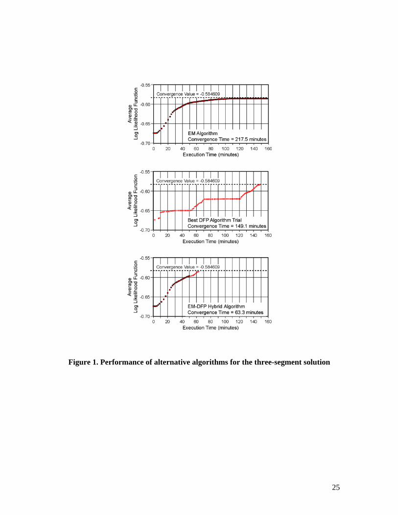
Figure 1. Performance of alternative algorithms for the three-segment solution
25
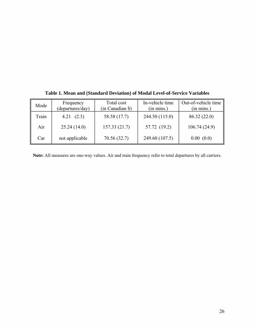
Table 1. Mean and (Standard Deviation) of Modal Level-of-Service Variables
Mode Frequency (departures/day)
Total cost (in Canadian $)
In-vehicle time (in mins.)
Out-of-vehicle time (in mins.)
Train 4.21 (2.3) 58.58 (17.7) 244.50 (115.0) 86.32 (22.0)
Air 25.24 (14.0) 157.33 (21.7) 57.72 (19.2) 106.74 (24.9)
Car not applicable 70.56 (32.7) 249.60 (107.5) 0.00 (0.0)
Note: All measures are one-way values. Air and train frequency refer to total departures by all carriers.
26
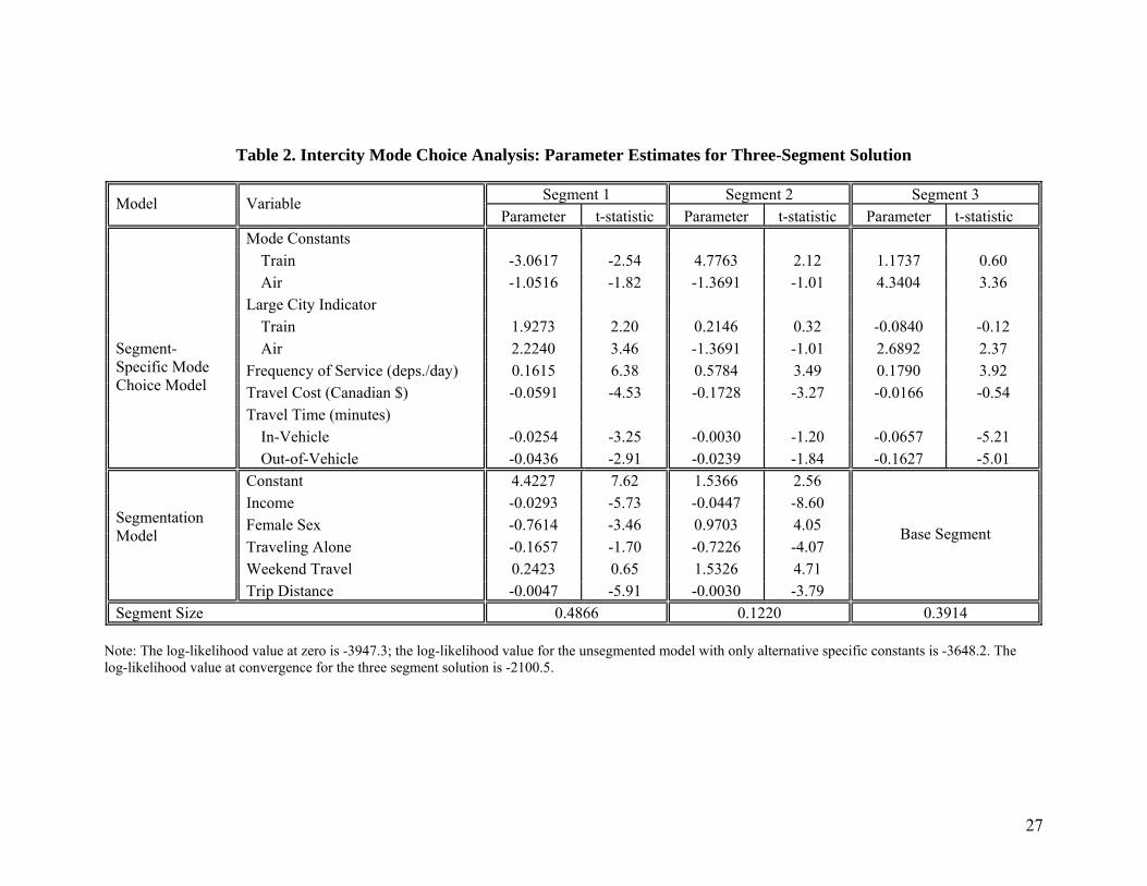
Table 2. Intercity Mode Choice Analysis: Parameter Estimates for Three-Segment Solution
Segment 1 Segment 2 Segment 3 Model
VariableParameter t-statistic Parameter t-statistic Parameter t-statistic
Mode Constants Train -3.0617 -2.54 4.7763 2.12 1.1737 0.60Air -1.0516 -1.82 -1.3691 -1.01 4.3404 3.36
Large City Indicator Train 1.9273 2.20 0.2146 0.32 -0.0840 -0.12Air 2.2240 3.46 -1.3691 -1.01 2.6892 2.37
Frequency of Service (deps./day) 0.1615 6.38 0.5784 3.49 0.1790 3.92 Travel Cost (Canadian $) -0.0591 -4.53 -0.1728 -3.27 -0.0166 -0.54 Travel Time (minutes)
In-Vehicle -0.0254 -3.25 -0.0030 -1.20 -0.0657 -5.21
Segment-Specific Mode Choice Model
Out-of-Vehicle -0.0436 -2.91 -0.0239 -1.84 -0.1627 -5.01Constant 4.4227 7.62 1.5366 2.56Income -0.0293 -5.73 -0.0447 -8.60Female Sex -0.7614 -3.46 0.9703 4.05 Traveling Alone -0.1657 -1.70 -0.7226 -4.07Weekend Travel 0.2423 0.65 1.5326 4.71
Segmentation Model
Trip Distance -0.0047 -5.91 -0.0030 -3.79
Base Segment
Segment Size 0.4866 0.1220 0.3914 Note: The log-likelihood value at zero is -3947.3; the log-likelihood value for the unsegmented model with only alternative specific constants is -3648.2. The log-likelihood value at convergence for the three segment solution is -2100.5.
27
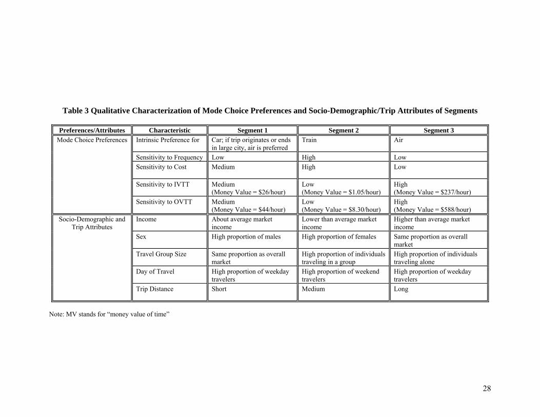
Table 3 Qualitative Characterization of Mode Choice Preferences and Socio-Demographic/Trip Attributes of Segments
Preferences/Attributes Characteristic Segment 1 Segment 2 Segment 3 Intrinsic Preference for Car; if trip originates or ends
in large city, air is preferred Train Air
Sensitivity to Frequency Low High Low Sensitivity to Cost
Medium High Low
Sensitivity to IVTT Medium (Money Value = $26/hour)
Low (Money Value = $1.05/hour)
High (Money Value = $237/hour)
Mode Choice Preferences
Sensitivity to OVTT Medium (Money Value = $44/hour)
Low (Money Value = $8.30/hour)
High (Money Value = $588/hour)
Income
About average market income
Lower than average market income
Higher than average market income
Sex High proportion of males High proportion of females Same proportion as overall market
Travel Group Size Same proportion as overall market
High proportion of individuals traveling in a group
High proportion of individuals traveling alone
Day of Travel High proportion of weekday travelers
High proportion of weekend travelers
High proportion of weekday travelers
Socio-Demographic and Trip Attributes
Trip Distance
Short Medium Long
Note: MV stands for “money value of time”
28
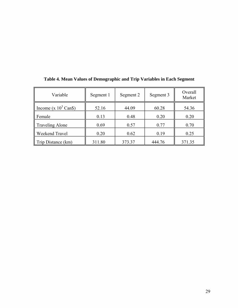
Table 4. Mean Values of Demographic and Trip Variables in Each Segment
Variable Segment 1 Segment 2 Segment 3 Overall Market
Income (x 103 Can$) 52.16 44.09 60.28 54.36
Female 0.13 0.48 0.20 0.20
Traveling Alone 0.69 0.57 0.77 0.70
Weekend Travel 0.20 0.62 0.19 0.25
Trip Distance (km) 311.80 373.37 444.76 371.35
29
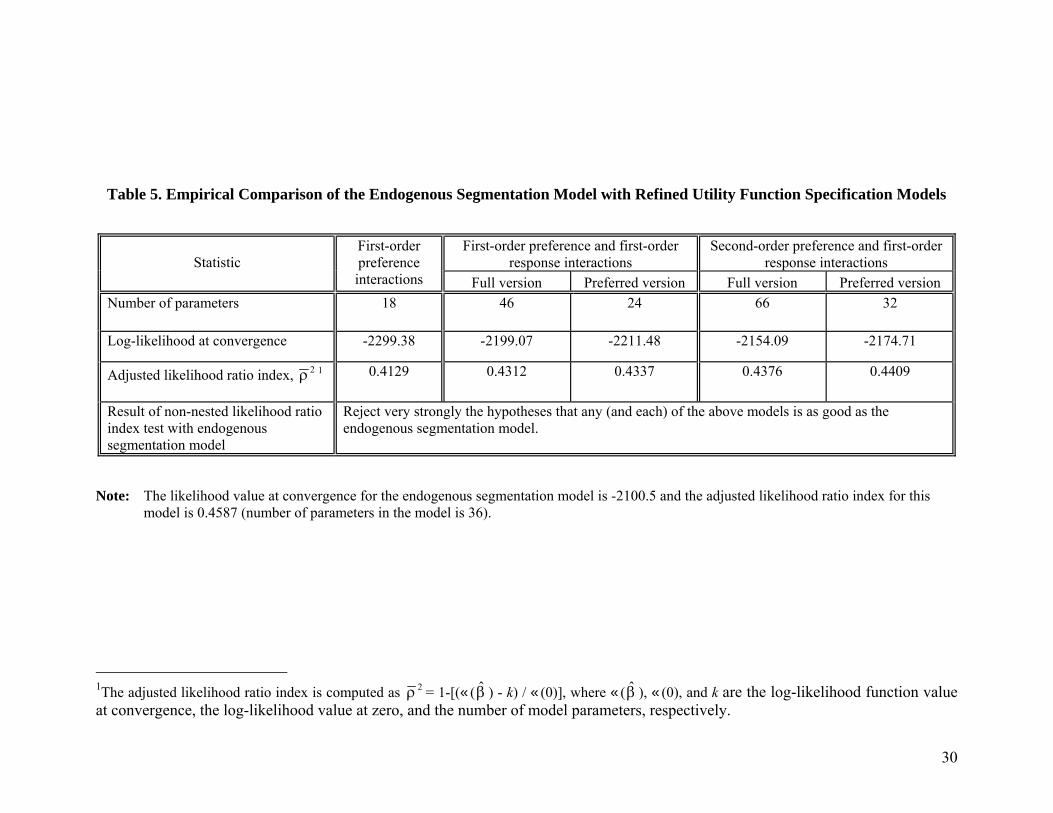
Table 5. Empirical Comparison of the Endogenous Segmentation Model with Refined Utility Function Specification Models
First-order preference and first-order response interactions
Second-order preference and first-order response interactions Statistic
First-order preference interactions Full version Preferred version Full version Preferred version
Number of parameters 18 46 24 66 32
Log-likelihood at convergence -2299.38 -2199.07 -2211.48 -2154.09 -2174.71
Adjusted likelihood ratio index, 2ρ 1 0.4129 0.4312 0.4337 0.4376 0.4409
Result of non-nested likelihood ratio index test with endogenous segmentation model
Reject very strongly the hypotheses that any (and each) of the above models is as good as the endogenous segmentation model.
Note: The likelihood value at convergence for the endogenous segmentation model is -2100.5 and the adjusted likelihood ratio index for this
model is 0.4587 (number of parameters in the model is 36).
1The adjusted likelihood ratio index is computed as 2ρ = 1-[(‹( ) - k) / ‹(0)], where ‹( ), ‹(0), and k are the log-likelihood function value at convergence, the log-likelihood value at zero, and the number of model parameters, respectively.
β̂ β̂
30
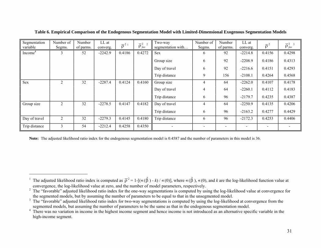
Table 6. Empirical Comparison of the Endogenous Segmentation Model with Limited-Dimensional Exogenous Segmentation Models
Segmentation variable
Number of Segms.
Number of parms.
LL at converg.
2ρ 1 2favρ 2 Two-way
segmentation with… Number of
Segms. Number of parms.
LL at converg.
2ρ 2favρ 3
Sex 6 92 -2214.8 0.4156 0.4298
Group size 6 92 -2208.9 0.4186 0.4313
Day of travel 6 92 -2216.6 0.4151 0.4293
Income4 3 52 -2242.9 0.4186 0.4272
Trip distance 9 156 -2108.1 0.4264 0.4568
Group size 4 64 -2262.0 0.4107 0.4178
Day of travel 4 64 -2260.1 0.4112 0.4183
Sex 2 32 -2287.4 0.4124 0.4160
Trip distance 6 96 -2179.7 0.4235 0.4387
Day of travel 4 64 -2250.9 0.4135 0.4206 Group size 2 32 -2278.5 0.4147 0.4182
Trip distance 6 96 -2163.2 0.4277 0.4429
Day of travel 2 32 -2279.3 0.4145 0.4180 Trip distance 6 96 -2172.3 0.4253 0.4406
Trip distance 3 54 -2212.4 0.4258 0.4350 - - - - - -
Note: The adjusted likelihood ratio index for the endogenous segmentation model is 0.4587 and the number of parameters in this model is 36.
1 The adjusted likelihood ratio index is computed as 2ρ = 1-[(‹( ) - k) / ‹(0)], where ‹( ), ‹(0), and k are the log-likelihood function value at
convergence, the log-likelihood value at zero, and the number of model parameters, respectively. β̂ β̂
2 The “favorable” adjusted likelihood ratio index for the one-way segmentations is computed by using the log-likelihood value at convergence for the segmented models, but by assuming the number of parameters to be equal to that in the unsegmented model.
3 The “favorable” adjusted likelihood ratio index for two-way segmentations is computed by using the log-likelihood at convergence from the segmented models, but assuming the number of parameters to be the same as that in the endogenous segmentation model.
4 There was no variation in income in the highest income segment and hence income is not introduced as an alternative specific variable in the high-income segment.
31
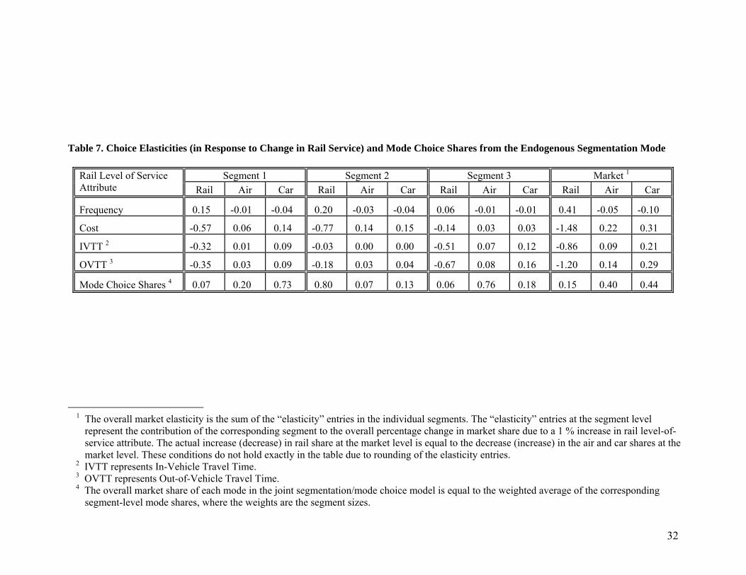
Table 7. Choice Elasticities (in Response to Change in Rail Service) and Mode Choice Shares from the Endogenous Segmentation Mode
Segment 1 Segment 2 Segment 3 Market 1Rail Level of Service Attribute Rail Air Car Rail Air Car Rail Air Car Rail Air Car
Frequency 0.15 -0.01 -0.04 0.20 -0.03 -0.04 0.06 -0.01 -0.01 0.41 -0.05 -0.10
Cost -0.57 0.06 0.14 -0.77 0.14 0.15 -0.14 0.03 0.03 -1.48 0.22 0.31
IVTT 2 -0.32 0.01 0.09 -0.03 0.00 0.00 -0.51 0.07 0.12 -0.86 0.09 0.21
OVTT 3 -0.35 0.03 0.09 -0.18 0.03 0.04 -0.67 0.08 0.16 -1.20 0.14 0.29
Mode Choice Shares 4 0.07 0.20 0.73 0.80 0.07 0.13 0.06 0.76 0.18 0.15 0.40 0.44
1 The overall market elasticity is the sum of the “elasticity” entries in the individual segments. The “elasticity” entries at the segment level
represent the contribution of the corresponding segment to the overall percentage change in market share due to a 1 % increase in rail level-of-service attribute. The actual increase (decrease) in rail share at the market level is equal to the decrease (increase) in the air and car shares at the market level. These conditions do not hold exactly in the table due to rounding of the elasticity entries.
2 IVTT represents In-Vehicle Travel Time. 3 OVTT represents Out-of-Vehicle Travel Time. 4 The overall market share of each mode in the joint segmentation/mode choice model is equal to the weighted average of the corresponding
segment-level mode shares, where the weights are the segment sizes.
32