Targeted Search, Endogenous Market Segmentation, and WageInequality

Huanxing Yang∗†

Department of Economics, Ohio State University

First Version: December 2015This Version: Feburary 2016

Abstract

Is it possible that the Internet has contributed to the rising wage inequality in the lasttwo decades? To answer this question, we develop a labor search/matching model withheterogeneous workers (a continuum of types) and heterogeneous firms (a finite number oftypes). One novel feature of our model is that search is targeted: each type of firms consti-tutes a distinctive submarket, and workers are able to choose beforehand which submarketto participate in, but search is random within each submarket, and wages are determinedby Nash bargaining. We show that, given the parameter values, there is always a uniqueequilibrium in which workers are endogenously segmented into different submarkets. Theequilibrium matching pattern is weakly positively assortative, with higher ability workersmatching with weakly more productive jobs. Moreover, the segmentation pattern affectsthe wage structure or wage distribution in the market. We then explore how the equilib-rium segmentation pattern and wage inequality change as some exogenous shocks occur,which includes a skill-biased technology progress in some high-productivity submarket anda decrease in the number of jobs in some low-productivity submarket. In particular, weshow that an Internet-induced increase in search effi ciency would make the matching pat-tern overall more assortatitve, increase wage inequality within each submarket (workerswith similar jobs), and also increase the overall wage inequality across submarkets.JEL: C78; D31; D83; J31Key Words: Targeted Search, Matching, Market Segmentation, Wage Inequality

1 Introduction

Since the late 1970s, the wage inequality in the U.S. has been steadily rising. One pronouncedfeature is that the skill premia of the high-skilled workers have continued to increase in thelast three decades. According to Autor et al. (2006), the wage inequality in the upper-tail(measured as the 90-50 percentile log-hourly wage differential) has increased steadily from

∗Eamil: yang.1041@osu.edu†I would like to thank David Blau, Yujing Xu, and the audience of the theory seminars at HKU, HKUST,

and MSU, for very helpful comments and suggestions. I also would like to thank Zhuozheng Li for excellentresearch assistance.

1

0.61 in 1973 to 0.81 in 2004. In absolute terms, Antonczyk et al. (2010) documented thatonly high-skilled workers (above the 80 percentile) have higher real wages in 2004 than in1979, while the real wages of workers below the 80 percentile actually decreased. The samepattern is also found in other developed countries (Dustmann et al. (2009) for Germany, andGoos and Manning (2007) for U.K.). The evolution of the wage inequality in the lower-tail issubtler. Autor et al. (2006) found that during the period 1973-2004, the wage inequality in thelower-tail (measured as the 50-10 percentile log-hourly wage differential) increased from 0.61 to0.69. However, after a sharp increase within 1973-1987, during 1988-2004 it actually decreased.Combining with the steady increase of inequality in the upper tail, the trend during 1988-2004was labeled as the “polarization” of wages. Nevertheless, the evidence of wage polarizationis restricted to the U.S.. In other industrialized countries, the wage inequality in the bottomhalf has been continuingly increasing. Antonczyk et al. (2010) also documented the trendsof wage inequality for specific skill groups in the U.S. during 1996-2004. They found thatamong low-skilled workers, the 80-50 difference were rather stable, but the 50-20 differenceslowly declined. As to medium-skilled workers, a clear pattern of wage polarization is found:the 80-50 difference has been increasing but the 50-20 difference has decreased. The wageinequality within high-skilled workers has been continuously increasing, both for the top andbottom half of the wage distribution.

The most prominent explanation for the rising wage inequality has been the skill-biasedtechnology change (Katz and Autor, 1999). In particular, a skill-biased technology changeincreases the demand for skilled workers and reduces that of unskilled ones, which tends toincrease wage inequality. In response to the evidence of wage polarization, a more sophisticatedversion of skill-biased technology change was developed recently (Autor et al., 2003, 2006, 2008;Goos and Manning, 2007). They argue that new technology (computerization for instance)favors highly skilled workers to less skilled routine-manual workers, and also favors less-skillednon-routine workers relative to less skilled routine-manual workers.1

This paper tries to provide an alternative explanation for the rising wage inequality. In par-ticular, could the widespread use of the Internet in the last two decades have contributed to therising wage inequality? For this purpose, this paper develops a labor search/matching modelwith heterogeneous workers and heterogeneous firms. Given that in the real world workers areof different abilities and firms have different productivities, who matches with who would nat-urally affect wage inequality. One novel feature of our model is that search is targeted: workersare able to choose beforehand which types of jobs to search (which submarket to participatein), but search is random within each submarket. Our model generates endogenous segmenta-tion of workers, with higher ability workers searching for (weakly) more productive jobs. Thesegmentation pattern affects the wage structure or wage distribution in the market. We thenexplore how the segmentation pattern and wage inequality change as some exogenous shocksoccur, including skill-biased technology changes and an Internet-induced increase in search ef-ficiency. One of our main results is that an Internet-induced increase in search effi ciency wouldmake the matching pattern overall more assortative and increase wage inequality.

The main ingredients of the model are as follows. Workers have different abilities or types,and firms have different productivities. While firms’types are finite, workers’types are con-

1Other explanations for the rising wage inequality are deunionization, falling real minimum wages, andchanges in the composition of labor force (DiNardo et al., 1996; Lemieux, 2006).

2

tinuous. Each firm demands exactly one worker. When a worker matches with a firm, theoutput is supermodular in the worker’s type and the firm’s type, except for the lowest typefirms, where the output does not depend on workers’types. The model is set in continuoustime. Unemployed workers search for job vacancies. Search is neither completely random, norcompletely directed. It lies somewhere in between (partially random and partially directed),and we label it as targeted search. In particular, each type of firms constitutes a distinctivesubmarket. Workers can choose which submarket to enter (or which type of firms to target).However, within each submarket, given the set of worker types participating in that submarket,search is random.

We assume an urn ball matching technology. That is, each type of worker always has thesame contact rate in any submarket. However, the meeting rate of unfilled job vacancies ina submarket depends on the market tightness in that submarket, which in turn depends onworkers’participating decisions. Once a worker meets a firm, the worker’s type is immediatelyobserved, and the firm decides whether to hire the worker. If the firm decides to hire, thewage is determined by Nash bargaining: split the surplus in the current match relative to bothparties’continuation values.

One key driving force of the model is the indirect externalities that workers within the samesubmarket impose on each other. The first kind of externality occurs among all workers. In aparticular submarket, more participating workers loosens the market tightness, which increasesfirms’contact rate and their continuation value. Due to Nash bargaining, this reduces the wagesfor all types of workers participating in that submarket. The second kind of externality is theone imposed by workers of high types on low type workers. Since search is random withineach submarket, Nash bargaining implies that firms’continuation value is corresponding toworkers’ average type. The presence of high type workers in a submarket (except for thelowest submarket) increases the average type. This increases firms’continuation value, which,again due to Nash bargaining, reduces the wages of the lower types in that submarket.

We establish that, given parameter values, there is always a unique market equilibrium.And the equilibrium features are as follows. First, workers are endogenously segmented (self-selected) into different submarkets. The endogenous segmentation exhibits weakly positivelyassortative matching: workers of higher types participate in weakly more productive sub-markets. The marginal types are indifferent between (get the same wage in) two adjacentsubmarkets. This is possible mainly due to the second kind of externality mentioned earlier:being the lowest type in a higher submarket reduces the worker’s share of the output, althoughthe higher submarket is more productive. The second equilibrium feature is that all submar-kets are interdependent. This is because the wages in any submarket depends on the set ofparticipating workers or marginal types of workers, but who are the marginal types in turndepends on the market conditions in adjacent submarkets. The final equilibrium feature is thatthe wage schedule (as a function of worker types) is piecewise linear and continuous: it is linearand increasing in type within each submarket, but is steeper in more productive submarkets.

We then conduct comparative statics. We first consider the impacts of a skill-biased technol-ogy progress. When the most productive jobs become more productive, in the most productivesubmarket all wages increase and the wage schedule becomes steeper. However, it also induceschanges in the endogenous segmentation: all the cutoff types decrease or matching overall be-

3

comes less assortative.2 As a result, wages of all types of workers (in all submarkets) increase.However, the wage increases are bigger for higher types. Therefore, a skill-biased technologyprogress not only increases the overall wage inequality across submarkets, but also increaseswage inequality within each submarket (among workers having similar jobs).

We then consider the case that some lower submarket loses jobs. This can be caused bymore intense international competition (for instance, cheap labor in China) or due to jobs beingreplaced by computers. Compared to the initial equilibrium, in the new equilibrium segmen-tation all the cutoff types in the submarkets higher than the one in question decrease, whileall the cutoff types in the lower submarkets increase. Wages of all types (in any submarket)decrease, and the wage decreases are bigger in submarkets that are closer to the submarketwhere the negative shock occurs. In a five submarkets case (high-tech, medium high-tech,medium, medium low-tech, and low-tech service jobs), if the negative shock occurs in themedium low-tech subsection, then it will increase the wage inequality in the upper tail (thethree higher submarkets), but reduces the wage inequality in the lower tail (medium low-tech,and low-tech service jobs), producing a pattern of wage polarization.

A combination of a skill-biased technology progress in the high-tech sector and a negativeshock in the medium low-tech sector can generate the following pattern. Wages in the twohighest submarkets increase, and the wage increases are bigger in the highest submarket. Wagesin the medium submarket are more or less the same. Wages in the two lowest submarketsdecrease, but the wage decreases are bigger in the medium low-tech sector. In short, in theupper tail both wages and wage inequality increase, while in the lower tail both wages andwage inequality decrease.

When a shock occurs in a middle submarket, we find that the transmissions of the shockto other submarkets through the changes in the endogenous segmentation exhibit asymmetry.Qualitatively, if the number of jobs in a middle submarket changes, then the adjustments inthe higher submarkets and those in the lower submarkets are always in the same direction: allwages either increase or decrease. However, if a skill-biased technology progress occurs in amiddle submarket, the adjustments in the higher submarkets and those in the lower submarketscould be in different directions: wages in the higher submarkets always increase, while thosein the lower submarkets might decrease. Quantitatively, the transmission of a shock to thehigher submarkets are always more significant than the transmission to the lower submarkets:the wage adjustments in higher submarkets are bigger while the wage adjustments in lowersubmarkets are smaller. For instance, if a skill-biased technology progress occurs in the mediumhigh-tech sector, then the wage increases in the two highest submarkets are significant, whilethe wage increases in the three lowest submarkets are negligible.

Finally, we study the impacts of a decrease in search friction. The widespread use of theInternet reduces workers’ search costs, which increases each worker’s contact rate. Anothereffect could be that the Internet reduces the probability of bad match in the horizontal dimen-sion (elaborated in Section 6), which, in terms of modeling, is equivalent to an increase in theeffective contact rate. As the search effi ciency/contact rate increases, if the initial equilibriumsegmentation were remaining the same, then in each submarket (except for the lowest one)the wages of higher type workers would increase, while those of lower types would decrease,

2 It means that there are fewer workers in the higher submarkets.

4

and the wage schedule would become steeper. This is because an increase in the contact ratedirectly increases each worker’s continuation value. However, it also increases firms’continu-ation value, which is roughly parallel to the average type workers’continuation value. Due toNash bargaining, in each submarket higher types gain and lower types lose. This pushes thelowest types in each submarket to the adjacent lower submarket.

Therefore, compared to the initial equilibrium, in the new equilibrium segmentation allthe cutoff types increase. In other words, the matching pattern becomes more assortative. Inthe new equilibrium, the wage schedule in each submarket (except for the least productiveone) becomes steeper. This means that the wage inequality within each submarket increases.Moreover, the wages of the highest types improve, while the wages of the lowest types decrease.Thus, the wage inequality across submarkets increases as well. This shows that the widespreaduse of the Internet in the last two decades could have contributed to the rising wage inequality.

In explaining the rising wage inequality, the models of skill biased technology change (seethe references mentioned earlier) typically treat different labor market sectors separately. Bydoing that, they do not capture how a shock in a particular market sector is transmittedto other market sectors. By endogenizing the market segmentation in a search/matchingframework, this paper captures the general equilibrium effects of sector-specific shocks: a shockin a particular submarket will be transmitted to other submarkets through the adjustment inendogenous segmentation.

There have been two search protocols in the labor search/matching literature.3 The firstone is random search, pioneered by Diamond (1982), Mortensen (1982), and Pissarides (1990).The second one is directed search, initially proposed by Peters (1991) and Montgomery (1991).In these early models, at least one side of the market is assumed to be homogeneous. Latermodels study the situation in which both workers and firms are heterogeneous. In particular,Shimer and Smith (2000) introduce search friction into Becker’s (1973) classical paper onmatching/assignment. In their model, both workers and firms have a continuum of types,and search is completely random. Their focus is on the form of the output function whichensures positively assortative matching, which turns out has to be log-supermodular. In adirected search model, Eeckhout and Kircher (2010) show that, by allowing firms to post pricesbeforehand to guide search, to ensure positively assortative matching the output function onlyneeds to be root-supermodular (also see Shi, 2001).

More related to our paper is Shimer (2005), who develops a one-period directed searchmodel with workers’ and firms’ types both being finite. In equilibrium, each worker typeplays mixed strategies (applying jobs of several types with positive probabilities). The maindifference between Shimer (2005) (and the directed search literature in general) and the currentpaper is that in his paper the coordination/congestion friction in the application process playsa central role. In our model, there is no direct coordination/congestion friction in the searchprocess, but workers within the same submarket impose indirect externalities on each otherthrough Nash bargaining. In spirit, our model resembles the models of competitive searchequilibrium (Shimer, 1996; Moen, 1997), in which firms of different productivities constitutedistinctive submarkets. The difference is that they are models of directed search (firms postwages beforehand), and workers are homogenous.

3See Rogerson et al. (2005) for a survey.

5

In the labor search/matching literature, the most closely related papers to our paper areAlbrecht and Vroman (2002) and Shi (2002), as they both study how skill biased technologyprogress affects the matching pattern and wage inequality. Both papers study a setting withtwo types of workers and two types of firms.4 In contrast, in our model workers’ types arecontinuous and firms have a finite number of types, which leads to a richer wage structure andallows us to map predictions more closely to empirical facts.5 In Albrecht and Vroman (2002),search is completely random, and high-skill jobs can only be performed by high-skill workers.Shi (2002) is a one-period directed search model, in which firms post wages beforehand todirect workers’application process. As mentioned earlier, the search/matching process in ourmodel is targeted, which lies somewhere in between directed search and random search. Inlater sections, we will further compare the differences in predictions between our model andtheir models.

One may wonder why we introduce a new search protocol of targeted search. The reasonsare twofold. First, compared to random search, targeted search is more realistic. In the realworld, we do see workers of different skills/abilities target different sets of jobs. For instance, thejobs applied by a PhD in economics typically do not overlap with those applied by a high schooldropout. Second, targeted search turns out to be more tractable than both random search anddirected search. In directed search models with both heterogeneous workers and heterogeneousfirms, firms offer type-dependent wages beforehand. And workers play mixed strategies, whichmeans that, for each type of workers, one needs to figure out the set of types of firms theworker applies to and the mixing probabilities. Moreover, workers’application strategies andfirms wage offers interact with each other, and workers’application strategies impose directexternalities on each other. Therefore, finding the equilibrium is a complicated process, letalone doing comparative statics.6 Compared to random search, perhaps it is surprising thattargeted search is more tractable. In random search models with heterogeneous workers andheterogeneous firms, for each worker type one needs to trace his acceptance set of firm types,and for each firm type one needs to trace the acceptance set of worker types. Moreover, theseacceptance sets interact with each other as they affect both sides’ continuation values. Asa result, it is very hard to fully characterize the equilibrium wage schedule and carry outcomparative statics.

In a search/matching model in the marriage market with non-transferable utilities, Burdettand Coles (1997) show that equilibrium exhibits block matching (weakly positively assortative).This feature is shared by the equilibrium matching pattern in our model, though in their modelsearch is completely random. Jacquet and Tan (2007) extend Burdett and Coles (1997) by

4 In a related paper, Acemogolu (1999) shows that an increase in the number of skilled workers might inducefirms to switch from offering “middling” jobs to offering specialized jobs. In his model, search is random andthere are only two types of workers.

5 In Shi (2002), high type workers only apply for high-tech jobs, while low type workers apply both high-techand low-tech jobs with positive probabilities. As a result, there are three different wages in total. In Albrechtand Vroman (2002), low type workers only match with low-tech jobs, while high type workers match with bothtypes of jobs. Again in total there are only three different wages.

6The complication is illustrated by Shimer (2005), and probably that is the reason why in his model botherworkers’and firms’types are finite. Moreover, the mixed strategy equilibrium in directed search models mightgenerate some features that are not very realistic. For instance, in Shimer (2005) the lowest type workers mightapply for the highest type job with a positive probability. In Shi (2002), the low type workers working inhigh-tech firms might get a higher actual wage than the high type workers working in high-tech firms.

6

allowing agents to choose who to meet with. That is, men and women are free to createsubmarkets. They show that this possibility makes the matching pattern more assortative.The feature that agents can choose who to meet with is related to the targeted search in ourmodel. The difference is that in our targeted search the submarkets are exogenously fixed(defined by firm types), and only workers choose which type of firms to meet with. In a sequel,Xu and Yang (2016) study a search/matching model in a marriage market with targeted searchand agents being horizontally differentiated.

In a labor market setting, a recent working paper by Cheremukhin et al. (2014) alsopropose a new search protocol of targeted search. While the terminology/labeling is the same,the targeted search in their model is very different from the one proposed in the currentpaper. In particular, their model emphasizes that agents have finite information processingcapacity, which limits agents’abilities to target their search to the best possible matches.7 Inour targeted search, such information processing costs do not exist: search is targeted simplymeans that workers are able to choose beforehand which submarket to participate in, andsearch is random within each submarket. The focuses of the two papers are also very different.While their paper focuses on the quality of the match,8 the current paper focuses on thematching pattern in the vertical dimension and wage inequality. In the context of consumersearch, Yang (2013) develops a targeted search model. In particular, he models targeted searchas the probability that a consumer type encounters the relevant goods in each search, which isexogenously determined by the Internet search technology. This is different from the targetedsearch in the current model, as consumers cannot choose beforehand which category of goodsto target.

The rest of the paper is organized as follows. Section 2 sets up the model. In Section 3 wecharacterize the market equilibrium. Section 4 studies the socially effi cient segmentation. InSections 5 and 6 we conduct the comparative statics: how the equilibrium matching patternand wage schedule change when some shocks occur. Section 7 offers conclusion and discussion.All the missing proofs in the text can be found in the Appendix.

2 Model

The model is set in continuous time, with r being the common discount rate.Consider a labor market with heterogeneous workers and heterogeneous firms. The measure

of workers is normalized to 1. Workers’abilities or skill levels (types) are indexed by x. Thesupport of x is [x, x], and its cumulative distribution function and density function are F (x)and f(x), respectively. We assume f(x) > 0 and it is continuous for all x ∈ [x, x]. There areN + 1 types of firms with different productivities, indexed by {0, 1, ..., N}. We assume N isfinite. A type n ≥ 1 firm’s productivity is θn, with 1 ≤ θ1 < ... < θN . The measure of type

7They show that, when the information process costs go to zero the matching outcome converges to that ofoptimal assignment, and when the information process costs go to infinity the matching outcome converges tothat of random search.

8 Implicitly, their model is more suitable for studying the situations in which the output is match-specific dueto horizontal differentiation among agents.

7

n firms is Yn; {Yn} are exogenously fixed, and 0 < Yn < 1 for all n.9 Each firm has exactlyone job. If a type x worker is matched with a type n (n ≥ 1) firm, then the flow output of thematch is θnx. Note that the production function is supermodular (for n ≥ 1), which meansthat from effi ciency point of view a higher type worker should be matched with a higher typefirm. If a type x worker is matched with a type 0 firm, the flow output is always 1 regardlessof the worker’s type. One can think of type 0 jobs as those only requiring basic skills (forinstance, low-tech service jobs).

Unemployed workers actively search for unfilled job vacancies.10 The search is not random.In particular, the labor market is segmented into N + 1 submarkets, with each type of firmsconstituting a distinctive submarket. The identity of each submarket (and hence firms’types)is always publicly observable. Each worker can choose which submarket or submarkets toparticipate in. If a worker chooses to participate in several submarkets, then he has to allocatehis search efforts across these submarkets. This setup resembles Moen’s (1997) directed searchmodel, in which firms of different productivities constitute different submarkets.

Each worker will only search in the submarkets which give him the highest expected utility.As will be shown later, generically, for any type x worker such a submarket is unique, and thushe will only search in one submarket. Let G(xn) and un be the type distribution of workertypes and the measure of unemployed workers, respectively, in submarket n. Denote vn as themeasure of unfilled vacancies in submarket n. Let qn ≡ un/vn be the expected queue lengthin submarket n, which is the inverse of the market tightness. We assume that the matchingfunction is generated by urn ball technology. In continuous time, at any instant of time thenumber of meetings in submarket n ism(un, vn) = αun, where α indicates the exogenous searchintensity of workers (Mortensen and Pissarides, 1999). Thus, the contact rate of a worker isalways α (in any submarket, as it is independent of the market tightness in any submarket).On the other hand, the contact rate of a type n firm is m(un, vn)/vn = αqn. Note that anincrease in qn leads to a higher contact rate for type n firms. Finally, if a type n firm meets aworker, the worker’s type is a random draw from G(xn). This is because all type n firms aresymmetric and all workers in submarket n have the same contact rate. In other words, searchis random within each submarket.11

Once an unfilled vacancy and an unemployed worker meet, the firm immediately observesthe worker’s type. Then the worker and the firm bargain for the wage and decide whether tomatch. The firm might reject the worker if the worker’s type x is too low. If both agree tomatch, then the match is consummated and they leave the market. Denote wn(x) as the wagepaid to the worker in a match between a type x worker and a type n firm. The wage wn(x) isdetermined by Nash bargaining, with the worker’s share of surplus being β. Specifically, denoteUn(x) as the expected discounted utility of a type x unemployed worker searching in submarketn, and En(x) as the expected discounted utility of a type x worker currently matched with atype n firm. Similarly, denote Vn as the expected discounted profit of an unfilled vacancy of

9Later on we will discuss how free entry affects the main results of the model.10There is no on-job search.11Suppose a worker participate in several submarkets. Specifically, suppose he randomizes his participation

decision accroding to σ, with σn,∑

n σn = 1, indicates his randomization probability in submarket n. Then hiscontact rate in submarket n is ασn. One can interpret that the worker spreads his search effort/time across thesubmarkets accroding σ.

8

type n firms, and Jn(x) as the expected discounted profit of a type n firm who is currentlymatched with a type x worker. Nash bargaining require that the wage wn(x) be implicitlydetermined by

En(x)− Un(x) = β[En(x) + Jn(x)− Un(x)− Vn]. (1)

All existing matches, regardless of workers’types and firms’types, have the same exogenousseparation rate δ. All unemployed workers get the same flow unemployment benefit b. Weassume that b < 1, which implies that it is effi cient for all workers to be employed (even bythe least productive jobs).

Two remarks are in order. First, the urn ball meeting technology implies that there is nodirect coordination/congestion friction on worker’s search: each worker’s contact rate does notdepend on the market tightness in each submarket. This is different from the directed searchliterature, where the direct coordination/congestion friction plays a central role. Second, searchis not random as workers are able to choose beforehand which submarket to participate in.However, search is not completely directed either. First of all, firms do not post wages before-hand to direct/guide search. Moreover, within the same submarket, each worker, regardlessof his type, always has the same contact rate, and a worker of a higher type does not have ahigher probability getting hired than a lower type worker, as long as firms in that submarketaccept both workers. This is because in continuous time, at any instant the probability that anunfilled vacancy gets two contacts from two workers, relative to the probability that an unfilledvacancy gets one contact, is negligible.12 Loosely put, in the current model, search is directedacross submarkets, but random within each submarket. To distinguish from the literature ofrandom search and that of directed search, we label our search protocol as targeted search.

3 Market Equilibrium

3.1 Preliminary analysis

A worker’s strategy is to choose which submarket to participate in, which is a mapping from histype x to the set of submarkets. A strategy profile of all workers is equivalent to a segmentationof workers’type space into different submarkets. We denote a segmentation as P : [x, x] →{0, 1, ..., N}. Let xn be the set of worker types who participate in submarket n. Thus, {xn}Nn=0,which exhausts the type space [x, x], also represents a segmentation. Let Xn be the measureof xn. The distribution of worker types within xn, G(xn), can be derived correspondingly fromF (x).

Given a segmentation P , in each submarket n the market conditions, xn, Xn, and G(xn),are all determined. In the ensuing search/matching process, along with Nash bargaining, thesemarket conditions determine wages in submarket n. Given the market conditions in submarketn, a type n firm’s strategy is a decision rule as to whether to accept a type x, x ∈ xn, worker ifthey meet. We first investigate the determination of wages wn(x) in each individual submarketn, given market conditions xn, Xn, and G(xn). In the process, we assume that type n firmsaccept all worker types x ∈ xn, as it will be shown to be an equilibrium feature later.12This is different from Shi’s (2002) one-period directed search model. In his model, a high-tech job might

get multiple applications from different types of workers, and thus the high type applicant has the priority toget empolyed.

9

Let mn be the measure of matched workers (firms as well) in submarket n. Then, we havethe following equations

mn + un = Xn; mn + vn = Yn; αun = δmn.

In particular, the third equation is the steady state condition: the number of newly formedmatches equals to that of destroyed matches. Given Xn, the above three equations uniquelydetermine the steady state un, vn, and qn:

un =Xnαδ + 1

, vn = Yn −αδXnαδ + 1

;

qn =Xn

[αδ + 1]Yn − αδXn

. (2)

Note that since all workers active in the same submarket, regardless of their types, havethe same matching rate, and all existing matches have the same break-up rate, the distributionof worker types in the unmatched pool must be the same as the distribution of worker typesactive in submarket n. That is, both are G(xn).

In submarket n ≥ 1, a type x worker’s value functions are given by

rUn(x) = b+ α[En(x)− Un(x)],

rEn(x) = wn(x) + δ[Un(x)− En(x)].

In the equation of Un(x), b is the flow payoff when unemployed. With rate α the worker hasa successful match (recall we assume type n firms accept all workers active in submarket n),in that case the worker enjoys an increase in value En(x)−Un(x). In the equation En(x), theworker’s flow payoff is wn(x). And with rate δ the current match is destroyed, and the workersuffers a loss Un(x)− En(x).

By similar logic, type n ≥ 1 firms’value functions are given by

rVn = αqn{Exn [Jn(x)]− Vn},rJn(x) = (θnx− wn(x)) + δ[Vn − Jn(x)].

In the equation of Vn, a firm’s successful match rate is αqn. Note that type n firms’optimalstrategy regarding whether to accept a worker is: accept a type x worker if and only if Jn(x) ≥Vn.

Submarket 0 is a little special in that the output does not depend on workers’types. Thus,type 0 firms always accept all types of workers. We can simplify the value functions as

rU0 = b+ α[E0 − U0], rE0 = w0 + δ[U0 − E0],

rV0 = αq0[J0 − V0], rJ0 = (1− w0) + δ(V0 − J0).

Applying the Nash bargaining equation (1), we have E0 − U0 = β[E0 + J0 − U0 − V0]. Fromthese equations, we get

w0 =(1− β)[r + δ + αq0]b+ β[r + δ + α]

r + δ + βα+ (1− β)αq0, (3)

10

which is uniquely determined given q0. From the expression of w0 (3), it can be immediatelyverified that w0 > b. This is because the output of type 0 job is 1, which is bigger than b, andworkers can always get a fraction of the surplus 1− b due to Nash bargaining.

Manipulating the value functions and the Nash bargaining equation (1), we get

rUn(x) = b+α[wn(x)− b]r + δ + α

, (4)

wn(x) =β(r + δ + α)[θnx− rVn] + (1− β)(r + δ)b

r + δ + βα. (5)

By equation (4), for any given type x worker, the submarket n having the highest wn(x) alsogives him the highest expected life utility. This is because the matching rate for workers is thesame across all submarkets. Therefore, a type x worker will participate in the submarket thatgives him the highest wage wn(x). Observing equation (5), we see that wn(x) is proportionalto θnx − rVn, which represents the surplus created by a type x worker in the current match(θnx is the output, and rVn is type n firms’bargaining or fallback position).

Now we provide a definition of equilibrium in this economy, which we call market equilib-rium.

Definition 1 A market equilibrium is characterized by a segmentation P or {xn} which sat-isfies the following requirements. (i) Each type x worker, x ∈ xn, should have no incentive tounilaterally deviate to participating in a submarket different from n: for any n and any x ∈ xn,wn(x) ≥ wn′ (x) for any n′ 6= n. (ii) For any n and any x ∈ xn, type n firms have an incentiveto accept a worker of type x: Jn(x) ≥ Vn.

Given that the number of firm types is finite and workers’types are continuous, matchingmust be mixed: some submarkets must have heterogeneous worker types. We show that theequilibrium matching pattern is still weakly positively assortative, meaning that higher typeworkers participate in weakly higher submarkets.

Lemma 1 Consider two worker types x′ and x′′, x′ < x′′, and two submarkets n′ and n′′,n′ < n′′. In market equilibrium, (i) if a type x′ worker prefers submarket n′′ to submarketn′, then a type x′′ worker must strictly prefer submarket n′′ to submarket n′; (ii) if a typex′′ worker prefers submarket n′ to submarket n′′, then a type x′ worker must strictly prefersubmarket n′ to submarket n′′.

Proof. We only prove part (i), as the proof of part (ii) is similar. The fact that a type x′ workerprefers submarket n′′ to submarket n′ means that wn′′(x′) ≥ wn′(x′). By the wage equation (5),it implies that θn′′x′ − rVn′′ ≥ θn′x′ − rVn′ , which is equivalent to (θn′′ − θn′)x′ ≥ rVn′′ − rVn′ .Using the fact that x′′ > x′, we have (θn′′ − θn′)x′′ > rVn′′ − rVn′ , which by the wage equation(5) implies that wn′′(x′′) > wn′(x

′′). That is, a type x′′ worker must strictly prefer submarketn′′ to submarket n′.

Lemma 1 establishes a single-crossing property: in equilibrium a higher type worker mustmatch with a weakly higher type firm. This result is formally stated in the following proposi-tion.

11

Proposition 1 In market equilibrium the segmentation of worker types must be an intervalpartition: the type space [x, x] is partitioned into N+1 (maybe fewer) connected intervals, withhigher type workers participating in weakly higher submarkets.

Thus equilibrium exhibits weakly positively assortative matching. This result is quiteintuitive. Given Nash bargaining, a worker always gets a certain share of surplus created.Since the production technology is supermodular, the difference of the surplus created betweenany pair of types of jobs is always bigger for a higher type worker. Moreover, the bargainingposition (Vn) of any type n firms is fixed when bargain with workers (deviations of individualworker types will not affect E[xn], and hence Vn). Therefore, the wage difference between anypair of types of jobs is always bigger for a higher type worker, which naturally leads to weaklypositive assortative matching. Proposition 1 also implies that there are at most N types ofworkers who are indifferent between participating in two adjacent submarkets. For a genericworker type x, there is a unique submarket that he strictly prefers.

By Proposition 1, an equilibrium segmentation is characterized by a weakly increasingsequence of cutoff types {xn} (we adopt the convention that x = x0 and x = xN+1), x0 ≤x1... ≤ xN+1, such that a worker of type x chooses submarket n if and only if x ∈ [xn, xn+1].Moreover, the density function of xn is given by g(xn) = f(xn)

F (xn+1)−F (xn) , and the measure of xnis given by Xn = F (xn+1)− F (xn).

Now we explicitly solve for wn(x) and Vn, still assuming type n firms always accept anyworker type x ∈ [xn, xn+1]. From the value functions and the Nash bargaining equation (1),we have

[r + δ + α]wn(x) = (1− β)(r + δ)b+ β[r + δ + βα][θnx−αqn

r + δ + αqnExn [θnx− wn(x)].

Taking expectation of Exn [·] on both sides of the above equation, we get

Exn [wn(x)] =(1− β)[r + δ + αqn]b+ β[r + δ + α]θnExn [x]

r + δ + βα+ (1− β)αqn.

From the above equations, wn(x) can be explicitly solved as

wn(x) =(1− β)[r + δ + αqn]b+ β[r + δ + α]θn{x+ (1−β)αqn

r+δ+βα [x− Exn [x]]}r + δ + βα+ (1− β)αqn

. (6)

Sometimes, it is useful to write wn(x) as

wn(x) =(1− β)[r + δ + αqn]b− (1− β)αqn

β[r+δ+α]θnExn [x]r+δ+βα

r + δ + βα+ (1− β)αqn+β[r + δ + α]

r + δ + βαθnx (7)

Similarly, type n firms’value, Vn, can be explicitly derived as:

rVn =(1− β)αqn[θnExn [x]− b]r + δ + βα+ (1− β)αqn

. (8)

Several observations are in order. First, inspecting (8) we see that Vn depends on Exn [x],the average ability of workers active in submarket n. This is intuitive, as Nash bargaining

12

implies that a type n firm gets a proportion of the expected surplus created by matching witha random worker, which is precisely the average type in expectation. Second, it can be readilyverified that ∂Vn

∂qn> 0 and Vn converges to 0 as qn approaches 0. This is also intuitive, since

an increase in qn means that firms’matching rate increases, which improves firms’position.When qn approaches 0, type n firms’matching rate also approaches 0, and as a result Vn tendsto 0. Third, by (7), we can immediately see that wn(x) is linear, and thus increasing, in x.Actually, the first term in (7) determines the intercept of the wage schedule wn(x), while thesecond term determines the slope. This is a direct consequence of the supermodular outputfunction and Nash bargaining. It follows immediately that the wage schedule wn(x) is steeperin a higher submarket. This is because the slope of the wage schedule wn(x),

∂wn(x)

∂x=β[r + δ + α]

r + δ + βαθn,

is increasing in θn. Finally, Jn(x) is increasing in x. To see this, by Nash bargaining equation(1) we can express Jn(x) as

Jn(x) =1− ββ

[wn(x)− b]r + δ + α

+ Vn. (9)

Since wn(x) is increasing in x, so is Jn(x). Again, this feature is due to Nash bargaining.

Lemma 2 (i) In each submarket n, wn(x) is decreasing in qn. (ii) In each submarket n ≥ 1,wn(x) is decreasing in Exn [x].

Proof. Both results follow immediately from (5) and the facts that ∂Vn∂qn> 0 and Vn is increasing

in Exn [x].The results for Lemma 2 are quite intuitive. An increase in qn or Exn [x] increases firms’

bargaining position Vn, which through Nash bargaining reduces the wages. Lemma 2 im-plies that within the same submarket workers impose indirect negative externalities on eachother by changing firms’bargaining position (recall that workers do not impose direct con-gestion/coordination externality on each other, as the meeting rate α is independent of themarket tightness 1/qn). In particular, there are two kinds of externalities. The first kind ofexternality occurs through qn, and thus exists among all workers. More workers active in asubmarket increases firms’matching rate and hence their bargaining position, which throughNash bargaining reduces the wages of all workers active in that submarket. The second kind ofexternality occurs through the channel of Exn [x], and thus is imposed by higher type workerson lower type workers. Specifically, the presence of higher type workers increases the averageability of workers, Exn [x], in submarket n, which improves firms’bargaining position Vn andreduces the wages of the lower type workers.

The negative externalities identified in Lemma 2 are the key driving forces of our model.This is because they are critical in pinning down the equilibrium segmentation. In particular,because of the second kind of externality, a worker of a relatively lower type x in submarket nmight be better off switching to submarket n − 1. To see this, note that in submarket n thistype suffers from the negative externality by being a lower type (a higher Vn, or x−Exn [x] < 0).

13

However, if this type participates in submarket n − 1, it becomes a higher type, and it cangain from a lower Vn−1 since x− Exn−1 [x] > 0.

Note that wn(x) reaches it upper bound wn(x) when qn = 0 (type x is the only type ofworker active in submarket n). By equation (5), they can be computed as:

wn(x) =β(r + δ + α)θnx+ (1− β)(r + δ)b

r + δ + βα,

w0 =β(r + δ + α) + (1− β)(r + δ)b

r + δ + βα.

It can be readily verified that wn(x) is increasing in n and x.To Summarize, a market equilibrium in this economy is characterized by the cutoff types

{xn}Nn=1. Given the cutoffs {xn}Nn=1 or an endogenous segmentation, the measures and thedistribution of worker types active in all submarkets, {Xn} and {G(xn)} are determined. Bythe steady state equations, {un}, {vn}, and {qn} are determined as well. Finally, from thevalue functions and the wage schedules, {wn(x)}, {Un(x)} and {Vn} are determined.

Let {x∗n}Nn=1 be the cutoff types in a market equilibrium. In light of the previous analysis,the two equilibrium conditions of market equilibrium now can be written as:

(i) The cutoff types of workers are indifferent between two adjacent submarkets: for alln = 1, ..., N ,

wn(x∗n) = wn−1(x∗n) if x∗n > x (interior cutoff), (10)

wn(x∗n) ≥ wn−1(x∗n) if x∗n = x (corner cutoff).

(ii) In any submarket n ≥ 1, no individual type n firm can strictly increase its Vn byaccepting only a strict subset of worker types within [x∗n, x

∗n+1].

Equilibrium requirement (i) is enough for no deviation on workers’part. This is becauseby Lemma 1, given that type x∗n is indifferent between submarkets n and n − 1, all workerswith type x > x∗n must strictly prefer submarket n to submarket n − 1, and all workers withtype x < x∗n must strictly prefer submarket n − 1 to submarket n. Equilibrium requirement(ii) applies to the lower worker types in each submarket, as it may not be rewarding for firmsif a worker’s type is too far below the average type of the existing pool. However, the followinglemma shows that equilibrium requirement (ii) is redundant if requirement (i) is satisfied.

Lemma 3 If equilibrium requirement (i) is satisfied, then equilibrium requirement (ii) is sat-isfied as well.

The underlying reason for Lemma 3 is that workers can anticipate firms’hiring behavior(criterion). If a worker’s type is too low compared to the average type of the existing pool insubmarket n such that type n firms do not accept him, the worker will simply participate insome less productive submarkets beforehand. More precisely, a type n firm is willing to accepta type x worker as long as θnx ≥ rVn + b (the output in the current match is bigger thanthe sum of outside options). But when this condition is binding, the worker’s wage is alreadypushed down to b, and the worker will switch to submarket 0 where he can get a wage w0 > b.This exactly means that workers’equilibrium participation decisions are more stringent than

14

firms acceptance decisions, thus equilibrium requirement (i) implies equilibrium requirement(ii). From now on, we can safely drop equilibrium requirement (ii).

Before investigating market equilibrium more closely, we first present a useful lemma.

Lemma 4 (i) Consider a type x′ worker in submarket n. Consider two scenarios in whichV ′n 6= V ′′n . Denote w

′n(x′) and w′′n(x′) as type x′ worker’s wage when type n firms have V ′n

and V ′′n , respectively. Then w′n(x′) > w′′n(x′) if and only if V ′n < V ′′n , and vice versa. (ii) In

submarket 0, w0 is strictly decreasing, and V0 is strictly increasing, in x1. (iii) In submarketN , VN is decreasing in xN ; VN is strictly decreasing in xN if type N firms accept type xN . (iv)In submarket n, 0 < n < N , consider two sets of participating worker types: [xn, xn+1] and[x′n, x

′n+1]. Denote type n firm’s equilibrium value in the first case and in the second case as Vn

and V ′n, respectively. If [xn, xn+1] v [x′n, x′n+1], then Vn ≤ V ′n. If xn+1 < x′n+1 and x

′n ≤ xn,

then Vn < V ′n. If xn+1 ≤ x′n+1 and x′n < xn and firms accept type x′n workers, then Vn < V ′n.

The results of Lemma 4 are intuitive. In any submarket, due to Nash bargaining, an increasein firms’continuation value Vn implies that any type x worker’s wage wn(x) decreases, and viceversa. In any submarket n, adding additional participating worker types will always weaklyimprove type n firms’value Vn, since it potentially increases firms’matching rate, and givesthem more options to choose among workers.

3.2 Existence and Uniqueness of Equilibrium

By equations (5) and (8), the indifference conditions of (10) can be explicitly written as: forall n = 1, ..., N , and x∗n > x,

(θn − θn−1)x∗n =(1− β)αqn[θnE(xn)− b]r + δ + βα+ (1− β)αqn

− (1− β)αqn−1[θnE(xn−1)− b]r + δ + βα+ (1− β)αqn−1

. (11)

Note that both qn and E[xn] are a function of x∗n and x∗n+1. Thus (11) is a second order

nonlinear difference equation, with boundary conditions x∗0 = x and x∗N+1 = x. Since thereis no general theorem regarding the existence and uniqueness of the solutions to second ordernonlinear difference equations, we have to establish them by ourselves.

Our method is by induction. In particular, we consider (partial) equilibrium within asubset of submarkets. For an exogenously given xn+1 ∈ (x, x), we investigate segmentations ofworker types within [x, xn+1] among submarkets 0, ..., n. Define x∗1,n+1(xn+1), ..., x∗n,n+1(xn+1)as the {xi}ni=1 such that all the submarkets below submarket n (including submarket n) arein (partial) equilibrium, or the indifference conditions of (10) for all i ≤ n are satisfied.13 Toabuse notation, we sometimes simply denote x∗i,n+1(xn+1), i = 1, ..., n, as x∗i . We start withn = 1.

Partial equilibrium in submarkets 0 and 1 Consider partial equilibria in submarkets 0and 1, given x2 ∈ (x, x). We will show that for any x2, x∗1 exists and is unique.

13Similarly, for an exogenously given xn ∈ (x, x), we can define the (partial) equilibrium segmentation ofworker types within [xn, x] among submarkets n, ..., N .

15

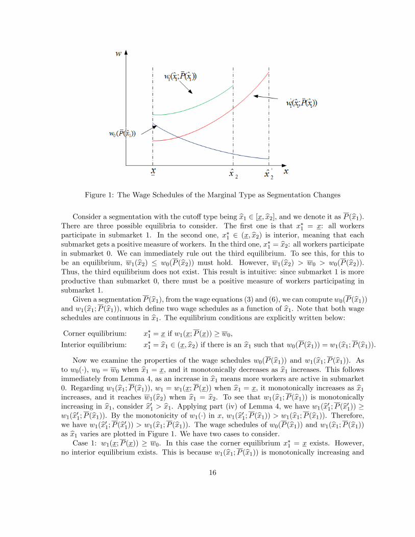
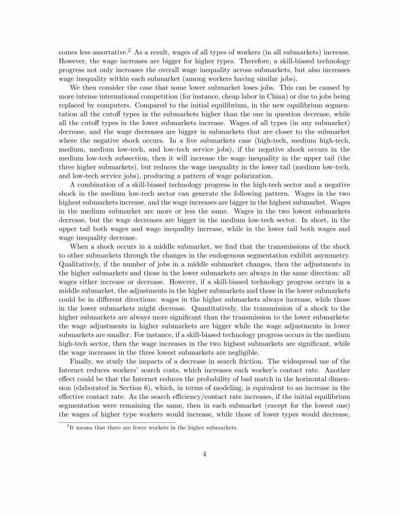
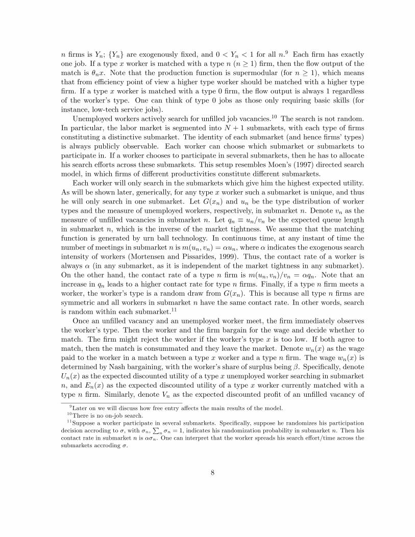
Figure 1: The Wage Schedules of the Marginal Type as Segmentation Changes

Consider a segmentation with the cutoff type being x1 ∈ [x, x2], and we denote it as P (x1).There are three possible equilibria to consider. The first one is that x∗1 = x: all workersparticipate in submarket 1. In the second one, x∗1 ∈ (x, x2) is interior, meaning that eachsubmarket gets a positive measure of workers. In the third one, x∗1 = x2: all workers participatein submarket 0. We can immediately rule out the third equilibrium. To see this, for this tobe an equilibrium, w1(x2) ≤ w0(P (x2)) must hold. However, w1(x2) > w0 > w0(P (x2)).Thus, the third equilibrium does not exist. This result is intuitive: since submarket 1 is moreproductive than submarket 0, there must be a positive measure of workers participating insubmarket 1.

Given a segmentation P (x1), from the wage equations (3) and (6), we can compute w0(P (x1))and w1(x1;P (x1)), which define two wage schedules as a function of x1. Note that both wageschedules are continuous in x1. The equilibrium conditions are explicitly written below:

Corner equilibrium: x∗1 = x if w1(x;P (x)) ≥ w0,

Interior equilibrium: x∗1 = x1 ∈ (x, x2) if there is an x1 such that w0(P (x1)) = w1(x1;P (x1)).

Now we examine the properties of the wage schedules w0(P (x1)) and w1(x1;P (x1)). Asto w0(·), w0 = w0 when x1 = x, and it monotonically decreases as x1 increases. This followsimmediately from Lemma 4, as an increase in x1 means more workers are active in submarket0. Regarding w1(x1;P (x1)), w1 = w1(x;P (x)) when x1 = x, it monotonically increases as x1

increases, and it reaches w1(x2) when x1 = x2. To see that w1(x1;P (x1)) is monotonicallyincreasing in x1, consider x′1 > x1. Applying part (iv) of Lemma 4, we have w1(x′1;P (x′1)) ≥w1(x′1;P (x1)). By the monotonicity of w1(·) in x, w1(x′1;P (x1)) > w1(x1;P (x1)). Therefore,we have w1(x′1;P (x′1)) > w1(x1;P (x1)). The wage schedules of w0(P (x1)) and w1(x1;P (x1))as x1 varies are plotted in Figure 1. We have two cases to consider.

Case 1: w1(x;P (x)) ≥ w0. In this case the corner equilibrium x∗1 = x exists. However,no interior equilibrium exists. This is because w1(x1;P (x1)) is monotonically increasing and

16

w0(P (x1)) is monotonically decreasing, in x1. Thus, the fact that w1(x;P (x)) ≥ w0 impliesthat the two wage schedules cannot have an interior intersection.14

Case 2: w1(x;P (x)) < w0. It is immediate that the corner equilibrium x1 = x cannotbe an equilibrium. Given that w1(x1;P (x1)) is monotonically increasing and w0(P (x1)) ismonotonically decreasing, in x1, the facts that w1(x;P (x)) < w0, w1(x2) > w0, and bothw1(x1;P (x1)) and w0(P (x1)) are continuous imply that the two wage schedules must have aunique intersection, which is interior. Therefore, in this case there is a unique equilibrium x∗1,which is interior: x∗1 ∈ (x, x2).15

Having established the existence and uniqueness of x∗1, now we investigate how x∗1 changesas x2 changes. Applying part (iv) of Lemma 4, as x2 increases, the whole wage schedule ofw1(·;P (·)) shifts downward (more workers active in submarket 1 pushes down w1(·;P (·))).16Moreover, as x2 increases the wage schedule of w0(P (·)) remains the same (just extends to alarger domain). This is because w0 only depends on the measure of workers active in submarket0. Therefore, from Figure 1 we reach two conclusions. First, there is a cutoff of x2, denotedas x#

2 , such that x∗1,2(x2) = x for all x2 ≤ x#

2 , and x∗1,2(x2) is interior if x2 > x#

2 . Second, if

x2 ≥ x#2 , then the interior equilibrium cutoff x∗1,2(x2) is strictly increasing in x2; if x2 < x#

2 ,then a marginal increase in x2 will not change the corner equilibrium.

Finally, as x2 increases to x′2 > x2, in the partial equilibrium we must have V ∗′1 > V ∗1 .To see this, consider three scenarios. In the first scenario, x2 < x#

2 and x′2 < x#2 (corner

equilibrium in both cases). Applying Lemma 4, it is immediate that V ∗′1 > V ∗1 . In the secondscenario, x2 ≤ x#

2 and x′2 > x#2 (corner equilibrium in the first case and interior equilibrium

in the second case). Suppose V ∗′1 ≤ V ∗1 . Then by Lemma 4, w′1(x∗′1 ) ≥ w1(x∗′1 ). In the originalequilibrium, we have w1(x∗′1 ) > w1(x) ≥ w0. Therefore, we get w′1(x∗′1 ) > w0, which meansthat x∗′1 cannot be the indifference type in the new equilibrium, a contradiction. In the thirdscenario, x2 > x#

2 and x′2 > x#2 (interior equilibrium in both cases). Again, suppose V ∗′1 ≤ V ∗1 .

Then by Lemma 4, w′1(x∗′1 ) ≥ w1(x∗′1 ). Since x∗′1 > x∗1, w1(x∗′1 ) > w1(x∗1) = w0. Thus, we havew′1(x∗′1 ) > w0. In submarket 0, the fact that x∗′1 > x∗1 implies, by Lemma 4, that w

′0 < w0.

Hence we have w′1(x∗′1 ) > w′0, which means that x∗′1 cannot be the indifference type in the new

equilibrium, a contradiction.The above results are summarized in the following lemma.

Lemma 5 Given any x2 ∈ (x, x), there is a unique x∗1 that achieves partial equilibrium insubmarkets 0 and 1. Moreover, in the partial equilibrium x∗1 is weakly increasing, and V

∗1 is

strictly increasing, in x2.

The intuition for these results is as follows. Workers always go for submarket 1 first, as itis more productive. But more workers there will push down the wages in submarket 1, leadingto some lower types switching to submarket 0. When some higher types exogenously switchfrom submarket 2 to submarket 1 (x2 increases), it pushes down the whole wage schedule insubmarket 1. To restore the indifference condition of the marginal type, the marginal typemust increase.14As illustrated in Figure 1 with x2.15As illustrated in Figure 1 with x′2.16As illustrated in Figure 1, with x2 < x′2, w

′1(·;P (·)) lies below w1(·;P (·)).

17

Partial equilibrium in submarkets 0, ..., n Now consider partial equilibria in submarkets0, ..., n, given xn+1 ∈ (x, x). Using induction, we show that, if the results of Lemma 5 hold forn− 1, then they also hold for n. This is formally stated in the following lemma.

Lemma 6 Suppose for n−1, given any xn ∈ (x, x), there is a unique equilibrium segmentation{x∗i }n−1

i=1 such that submarkets 0, ..., n−1 achieve partial equilibrium. Moreover, {x∗i }n−1i=1 are all

weakly increasing in xn−1, and V ∗n−1 is strictly increasing in xn. Then, given any xn+1 ∈ (x, x),there is a unique equilibrium segmentation {x∗i }ni=1 such that submarkets 0, ..., n achieve partialequilibrium. Moreover, in the partial equilibrium x∗n is increasing, and V

∗n is strictly increasing,

in xn+1.

Equilibrium in the whole market Given the results of Lemma 5, we can apply Lemma 6recursively. In each step, one more higher submarket is included. This step-by-step inductionwill eventually reach submarket N , which means that a market equilibrium in the whole marketexists and is unique. Thus, we have proved the following proposition.

Proposition 2 A market equilibrium exists. Moreover, given parameter values, the marketequilibrium is unique.

Lemma 5 and Lemma 6 also imply the following corollary, which will be useful in lateranalysis. Essentially, it says that if one cutoff changes for some exogenous reason, then torestore (partial) equilibrium in other submarkets, all other cutoffs must move in the samedirection.

Corollary 1 (i) If xn, 2 ≤ n ≤ N , increases, then {x∗i }n−1i=1 , which ensures submarkets

0, 1, ..., n−1 in partial equilibrium, all weakly increase; (ii) If xn, 1 ≤ n ≤ N−1, increases, then{x∗i }Ni=n, which ensures submarkets n, n+ 1, ..., N in partial equilibrium, all weakly increase.

Proof. Part (i) is directly implied by Lemma 5 and Lemma 6. Part (ii) can be proved in asimilar fashion, and thus is omitted.

The existence of market equilibrium is ensured because each worker type has to choosesome submarket to participate in. The underlying reason for the uniqueness of equilibrium isthe indirect negative externalities workers within the same submarket imposed on each other,which we emphasized earlier. Specifically, more workers active in a particular submarket nimprove type n firms’position and reduces the wages for all worker types participating in thatsubmarket. One other other hand, more workers active in submarket n means fewer workers inother submarkets, which increases the wages for workers participating in other submarkets. Inshort, more workers in submarket n reduces the attractiveness of submarket n, but increasesthe attractiveness of other submarkets, to workers. This indirect negative externality meansthat the segmentation has to be right in equilibrium to ensure no deviation on part of theworkers, which implies the uniqueness of equilibrium.

Intuitively, one can think that an equilibrium segmentation is reached from-top-to-down.First, the most able workers participate in submarket N , the most productive one. Gradually,as more marginally lower type workers participate in this submarket, type N firms’positionimproves, which pushes down the whole wage schedule in submarket N . At some point, the

18

marginally lower type workers’ wage in submarket N becomes too low, and they start toparticipate in submarket N − 1, the next most productive one. And the same process repeatsin submarket N − 1, and so on.

3.3 Equilibrium properties

Several equilibrium properties are worth mentioning. First, wages in individual submarketsare semi-independent but indirectly linked. Specifically, given a segmentation, wages in eachsubmarket are independently determined, as they only depend on the market condition intheir own submarket. However, in equilibrium all the submarkets are indirectly linked throughworkers’participation decisions. For instance, the wages in any two adjacent submarkets areinterdependent because the marginal type who is indifferent between these two submarketsdepends on the wages in both submarkets. Since the interdependence exists between any twoadjacent submarkets, all the submarkets are all indirectly linked. It means that if an exogenousshock occurs to any submarket, its impact will spread to all other submarkets, through theindirect links.

Second, in equilibrium, except for the lowest types participating in submarket 0, wage isincreasing in worker’s type. In particular, the equilibrium wage schedule is piecewise linearin workers’type: linear within each submarket, steeper in higher submarkets, but continuousacross submarkets.17 This implies that the wage schedule is weakly convex in worker’s type.18

Third, in equilibrium V ∗n must be increasing in n, or more productive job vacancies have ahigher value. This is because if V ∗n+1 ≤ V ∗n , then all workers in submarkets n+ 1 and n wouldhave preferred submarket n + 1 to submarket n.19 As to the expected queue length q∗n, thegeneral pattern is that q∗n should be increasing in n, as this helps to make the marginal type x

∗n

indifferent between submarkets n+1 and n. However, the difference between the average typesE(xn+1) and E(xn) can also help to make the marginal type x∗n indifferent. This implies thatq∗n is not necessarily monotonic. Instead, whether q

∗n is monotonic depends on the distribution

of worker types and the distribution of job types.

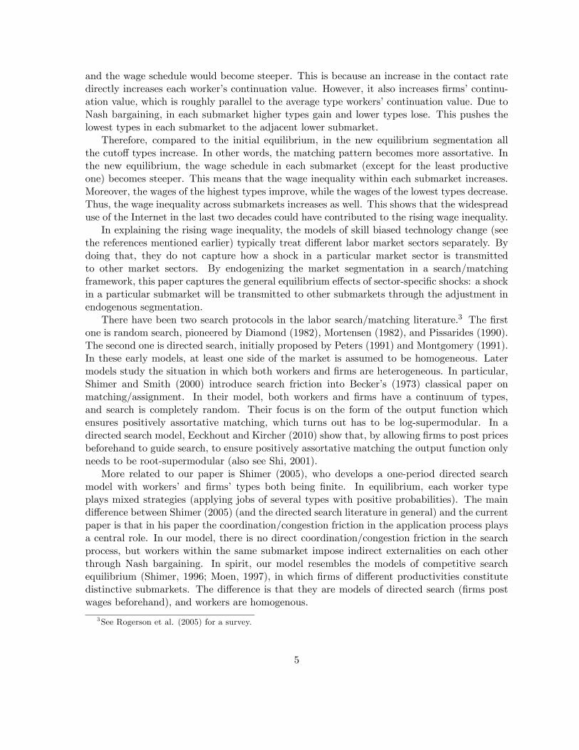
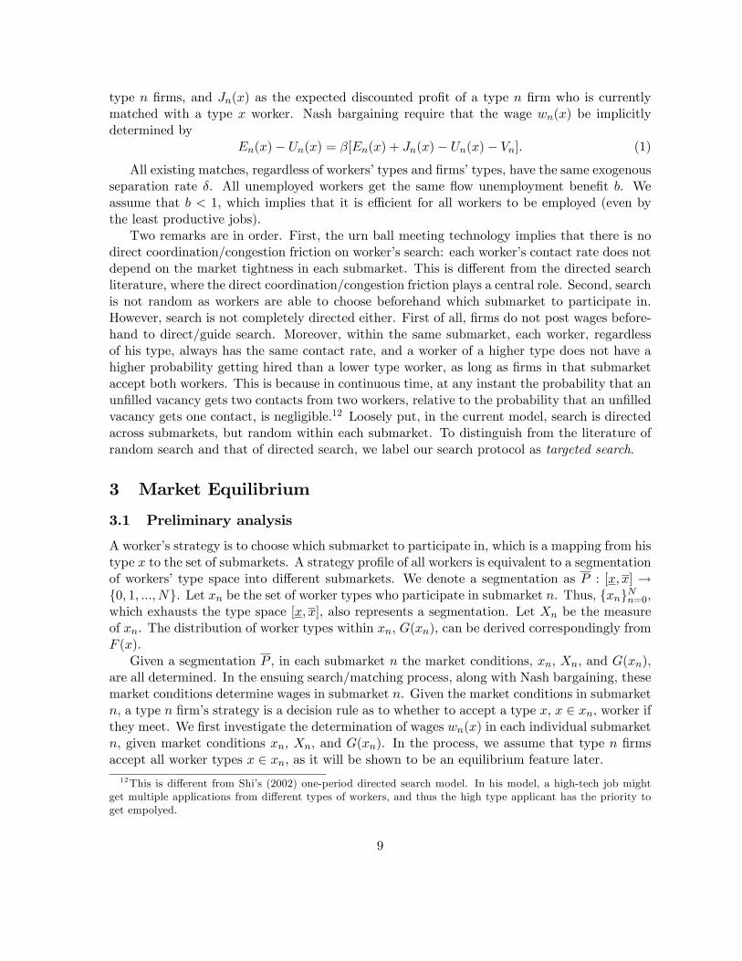
Example 1 (The benchmark case) Workers’type distribution is truncated normal on [0.5, 4],with mean 1.5 and variance 0.7.20 There are five types of firms. Firms’productivities (θ1, θ2, θ3, θ4) =(1, 1.5, 2, 2.5), and the measures of firms (Y0, Y1, Y2, Y3, Y4) = (0.25, 0.25, 0.2, 0.15, 0.1), withthe total measure of firms being 0.95.21 The other parameter values are: b = 0.5, r = 0.05,δ = 0.06, β = 0.65, and α = 0.1. The equilibrium wage schedule is illustrated in Figure 1(each submarket is of a different color). Workers’ type distribution and the equilibrium wagedistribution are illustrated in Figure 2, and the key endogenous variables are recorded in Table1.17The continuity in the wage schedule is due to the fact that each cutoff type is indifferent between two

adjacent submarkets.18 If the number of firm types goes to infinity, then the wage schedule will be close to being strictly convex.19More explictly, the indifference condition (11) can be written compactly as (θn − θn−1)x∗n = rV ∗n − rV ∗n−1.20We choose worker type distribution to be truncated normal because empirical evidence (see Herrnstein and

Murray, 1994) indicates that it is the case.21As mentioned in the introduction, these five submarkets are corresponding to high-tech, medium high-tech,

medium (manufacturing), medium low-tech (low-skill manufacturing), and low-tech service jobs. The measuresof these jobs are chosen to match the distribution of job types in the real world.

19

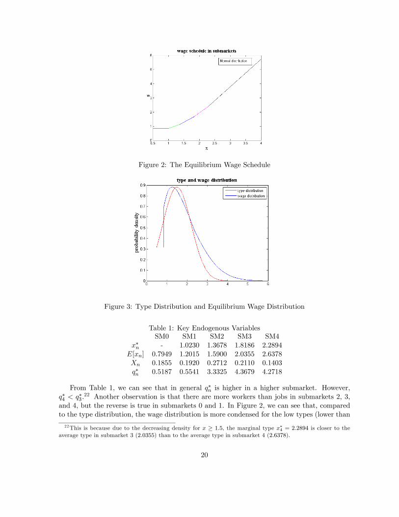
Figure 2: The Equilibrium Wage Schedule

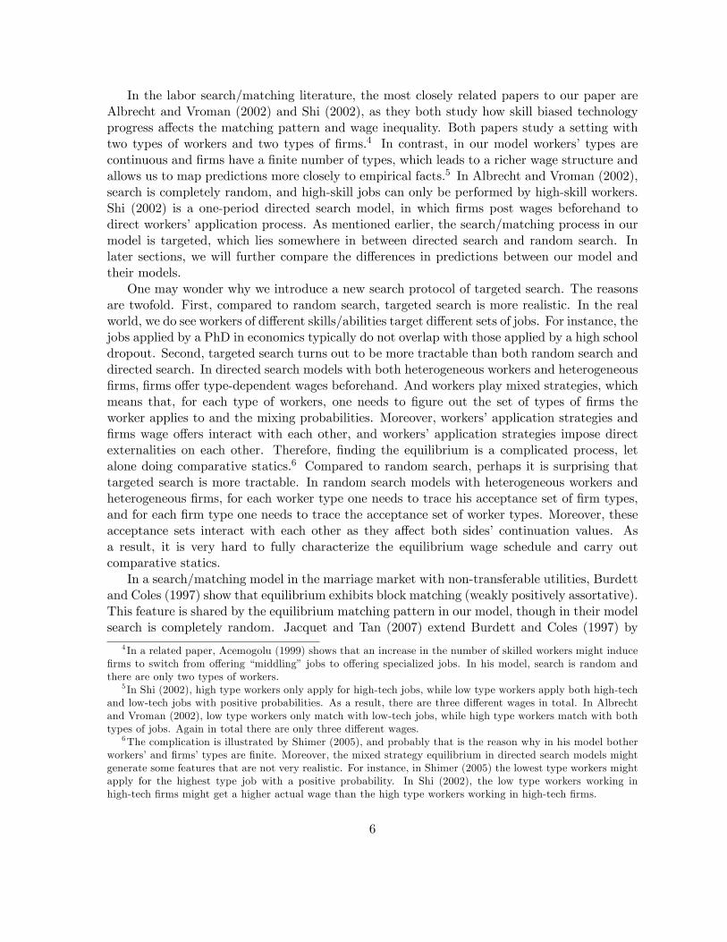
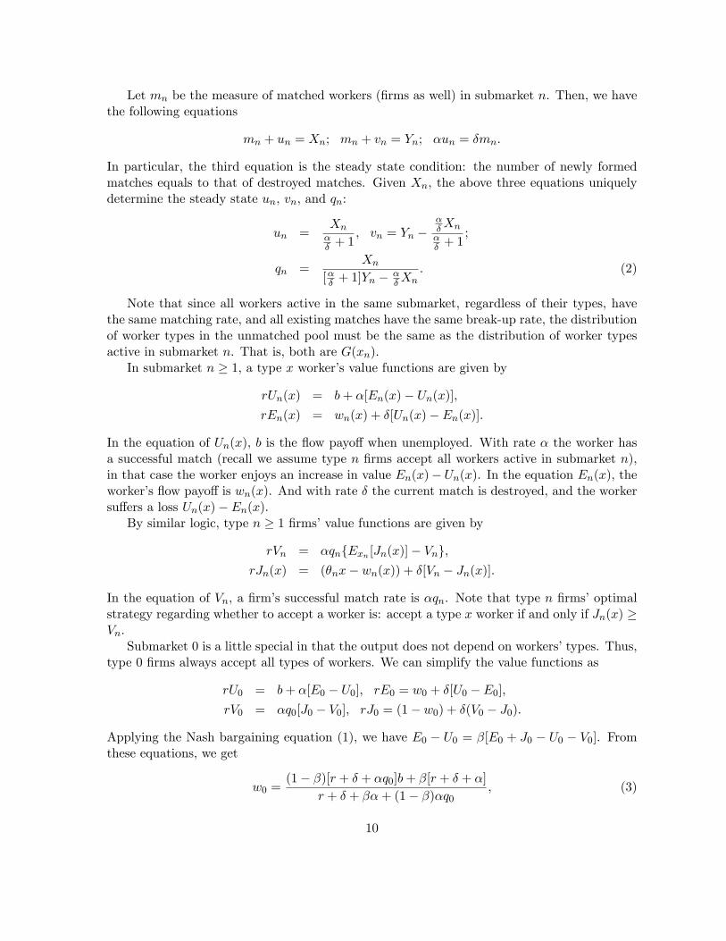
Figure 3: Type Distribution and Equilibrium Wage Distribution

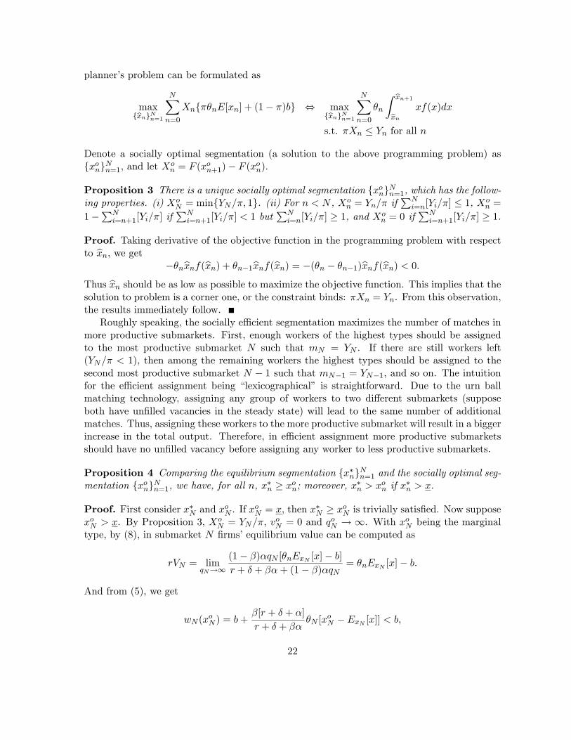
Table 1: Key Endogenous VariablesSM0 SM1 SM2 SM3 SM4

x∗n - 1.0230 1.3678 1.8186 2.2894E[xn] 0.7949 1.2015 1.5900 2.0355 2.6378Xn 0.1855 0.1920 0.2712 0.2110 0.1403q∗n 0.5187 0.5541 3.3325 4.3679 4.2718

From Table 1, we can see that in general q∗n is higher in a higher submarket. However,q∗4 < q∗3.

22 Another observation is that there are more workers than jobs in submarkets 2, 3,and 4, but the reverse is true in submarkets 0 and 1. In Figure 2, we can see that, comparedto the type distribution, the wage distribution is more condensed for the low types (lower than

22This is because due to the decreasing density for x ≥ 1.5, the marginal type x∗4 = 2.2894 is closer to theaverage type in submarket 3 (2.0355) than to the average type in submarket 4 (2.6378).

20

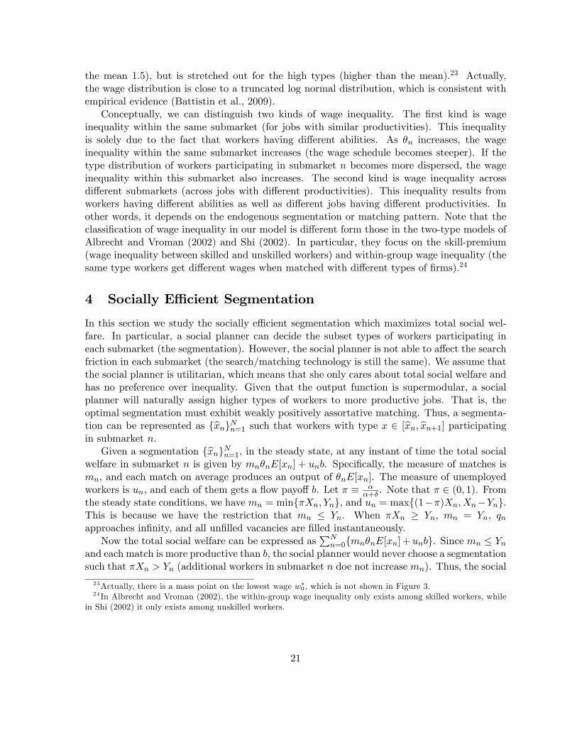
the mean 1.5), but is stretched out for the high types (higher than the mean).23 Actually,the wage distribution is close to a truncated log normal distribution, which is consistent withempirical evidence (Battistin et al., 2009).

Conceptually, we can distinguish two kinds of wage inequality. The first kind is wageinequality within the same submarket (for jobs with similar productivities). This inequalityis solely due to the fact that workers having different abilities. As θn increases, the wageinequality within the same submarket increases (the wage schedule becomes steeper). If thetype distribution of workers participating in submarket n becomes more dispersed, the wageinequality within this submarket also increases. The second kind is wage inequality acrossdifferent submarkets (across jobs with different productivities). This inequality results fromworkers having different abilities as well as different jobs having different productivities. Inother words, it depends on the endogenous segmentation or matching pattern. Note that theclassification of wage inequality in our model is different form those in the two-type models ofAlbrecht and Vroman (2002) and Shi (2002). In particular, they focus on the skill-premium(wage inequality between skilled and unskilled workers) and within-group wage inequality (thesame type workers get different wages when matched with different types of firms).24

4 Socially Effi cient Segmentation

In this section we study the socially effi cient segmentation which maximizes total social wel-fare. In particular, a social planner can decide the subset types of workers participating ineach submarket (the segmentation). However, the social planner is not able to affect the searchfriction in each submarket (the search/matching technology is still the same). We assume thatthe social planner is utilitarian, which means that she only cares about total social welfare andhas no preference over inequality. Given that the output function is supermodular, a socialplanner will naturally assign higher types of workers to more productive jobs. That is, theoptimal segmentation must exhibit weakly positively assortative matching. Thus, a segmenta-tion can be represented as {xn}Nn=1 such that workers with type x ∈ [xn, xn+1] participatingin submarket n.

Given a segmentation {xn}Nn=1, in the steady state, at any instant of time the total socialwelfare in submarket n is given by mnθnE[xn] + unb. Specifically, the measure of matches ismn, and each match on average produces an output of θnE[xn]. The measure of unemployedworkers is un, and each of them gets a flow payoff b. Let π ≡ α

α+δ . Note that π ∈ (0, 1). Fromthe steady state conditions, we have mn = min{πXn, Yn}, and un = max{(1−π)Xn, Xn−Yn}.This is because we have the restriction that mn ≤ Yn. When πXn ≥ Yn, mn = Yn, qnapproaches infinity, and all unfilled vacancies are filled instantaneously.

Now the total social welfare can be expressed as∑N

n=0{mnθnE[xn] +unb}. Since mn ≤ Ynand each match is more productive than b, the social planner would never choose a segmentationsuch that πXn > Yn (additional workers in submarket n doe not increase mn). Thus, the social

23Actually, there is a mass point on the lowest wage w∗0 , which is not shown in Figure 3.24 In Albrecht and Vroman (2002), the within-group wage inequality only exists among skilled workers, while

in Shi (2002) it only exists among unskilled workers.

21

planner’s problem can be formulated as

max{xn}Nn=1

N∑n=0

Xn{πθnE[xn] + (1− π)b} ⇔ max{xn}Nn=1

N∑n=0

θn

∫ xn+1

xn

xf(x)dx

s.t. πXn ≤ Yn for all n

Denote a socially optimal segmentation (a solution to the above programming problem) as{xon}Nn=1, and let X

on = F (xon+1)− F (xon).

Proposition 3 There is a unique socially optimal segmentation {xon}Nn=1, which has the follow-ing properties. (i) Xo

N = min{YN/π, 1}. (ii) For n < N , Xon = Yn/π if

∑Ni=n[Yi/π] ≤ 1, Xo

n =

1−∑N

i=n+1[Yi/π] if∑N

i=n+1[Yi/π] < 1 but∑N

i=n[Yi/π] ≥ 1, and Xon = 0 if

∑Ni=n+1[Yi/π] ≥ 1.

Proof. Taking derivative of the objective function in the programming problem with respectto xn, we get

−θnxnf(xn) + θn−1xnf(xn) = −(θn − θn−1)xnf(xn) < 0.

Thus xn should be as low as possible to maximize the objective function. This implies that thesolution to problem is a corner one, or the constraint binds: πXn = Yn. From this observation,the results immediately follow.

Roughly speaking, the socially effi cient segmentation maximizes the number of matches inmore productive submarkets. First, enough workers of the highest types should be assignedto the most productive submarket N such that mN = YN . If there are still workers left(YN/π < 1), then among the remaining workers the highest types should be assigned to thesecond most productive submarket N − 1 such that mN−1 = YN−1, and so on. The intuitionfor the effi cient assignment being “lexicographical” is straightforward. Due to the urn ballmatching technology, assigning any group of workers to two different submarkets (supposeboth have unfilled vacancies in the steady state) will lead to the same number of additionalmatches. Thus, assigning these workers to the more productive submarket will result in a biggerincrease in the total output. Therefore, in effi cient assignment more productive submarketsshould have no unfilled vacancy before assigning any worker to less productive submarkets.

Proposition 4 Comparing the equilibrium segmentation {x∗n}Nn=1 and the socially optimal seg-mentation {xon}Nn=1, we have, for all n, x

∗n ≥ xon; moreover, x∗n > xon if x

∗n > x.

Proof. First consider x∗N and xoN . If x

oN = x, then x∗N ≥ xoN is trivially satisfied. Now suppose

xoN > x. By Proposition 3, XoN = YN/π, voN = 0 and qoN → ∞. With xoN being the marginal

type, by (8), in submarket N firms’equilibrium value can be computed as

rVN = limqN→∞

(1− β)αqN [θnExN [x]− b]r + δ + βα+ (1− β)αqN

= θnExN [x]− b.

And from (5), we get

wN (xoN ) = b+β[r + δ + α]

r + δ + βαθN [xoN − ExN [x]] < b,

22

where the inequality follows because xoN < ExN [x]. The fact that wN (xoN ) < b implies that theequilibrium x∗N must be strictly greater than xoN , since in equilibrium we have wN (x∗N ) > b,and wN (xN ;P (xN )) is increasing in xN .

Now suppose the results hold for n+ 1. We want to show that the results also hold for n.If xon = x, then the statement is trivially satisfied. Now suppose xon > x. By a similar logicas in the previous step, we can show that, with worker types within [xon, x

on+1] participating

in submarket n, wn(xon;P (xon+1)) < b. Thus, x∗n(P (xon+1)) > xon(P (xon+1)) = xon. By Corollary1, x∗n = x∗n(P (x∗n+1)) > x∗n(P (xon+1)), since x∗n+1 > xon+1 by the presumption. Therefore,x∗n > xon.

Proposition 4 illustrates that, compared to the socially optimal segmentation, in equilib-rium too fewer workers are participating in more productive submarkets. Or loosely speaking,the equilibrium segmentation exhibits less assortative matching relative to the optimal seg-mentation. Intuitively, the equilibrium segmentation is determined by wage equalization formarginal types, while the effi cient segmentation is driven by output equalization for marginaltypes. Since output cannot be equalized for marginal types, effi cient segmentation leads to acorner solution. That is, the most productive submarkets are extremely loose (the queue lengthgoes to infinity) under the effi cient segmentation. This means that firms in these submarketshave a higher value (their vacancies are filled instantaneously), which drives down the wages ofthe marginal types below the unemployment benefit b. This implies that in equilibrium theremust be fewer workers participating in more productive submarkets than under the effi cientsegmentation.

5 Shocks to Individual Submarkets

In this section and the next section we investigate how the equilibrium, including the segmen-tation pattern, the wage schedule, and the tightness of individual submarkets, will change assome of the exogenous parameters vary. We focus on shocks to individual submarkets in thissection. In particular, we conduct two comparative statics analysis: a skill-biased technologyprogress in a more productive submarket, and a reduction in the number of jobs in some lessproductive submarket. To make the analysis clean, in the rest of the paper we focus on interiorequilibria: x∗1 > x. That is, each submarket has a positive measure of participating workers.We also denote we(x) as the equilibrium wage schedule. Note that we(x) depends on theequilibrium segmentation.

5.1 Skill-biased technology progress

To study the impacts of a skill biased technology progress, suppose θN increases to θ′N > θN ,while all the other parameters of the model remain the same. That is, the most-productive jobsbecome more productive. We use superscript “′” to denote the endogenous variables underθ′N .

To proceed, we first fix the original equilibrium segmentation pattern P , and investigate howan increase in θN upsets the original equilibrium. Since all other parameter values remain thesame and P remains the same, in all submarkets other than submarket N the wage schedules

23

and firms’values do not change either. Now consider submarket N . For any x ≥ x∗N , by (6),

∂wN (x, P )

∂θN∝ x+

(1− β)αqNr + δ + βα

[x− Exn [x]] > 0.

The inequality holds because in equilibrium wN (x) ≥ b, which by (6) implies that the aboveexpression is bigger than b. Thus, an increase in θN shifts the whole wage schedule up insubmarket N . This is intuitive, as by Nash bargaining the increases in outputs will be sharedby workers and firms. In particular, the wage of the original marginal type increases as well:w′N (x∗N , P ) > wN (x∗N , P ). But this means that type x∗N worker is no longer indifferent betweensubmarkets N−1 and N . Therefore, the original equilibrium segmentation will have to changein order to restore equilibrium.

Proposition 5 Suppose θN increases to θ′N > θN , while all the other parameters of the modelremain the same. Then, the following results hold. (i) x∗′n < x∗n for all n = 1, ..., N ; (ii)w′e(x) > we(x) for any x (the whole wage schedule shifts up); (iii) V ∗′n < V ∗n for n ≤ N − 1,and V ∗′N > VN ; (iv) u∗′1 < u∗1 and q

∗′1 < q∗1, and u

∗′N > u∗N and q∗′N > q∗N .

The results of Proposition 5 are intuitive. As type N firms become more productive, dueto Nash bargaining both the wages and firms’value in submarket N naturally increase. Thisattracts some high types in submarket N − 1 (just below the initial cutoff x∗N ) to switch tosubmarket N . This increases the market tightness in submarket N − 1, which improves wagesbut makes type N − 1 firms worse off. But this further attracts some high types in submarketN−2 (just below the cutoff x∗N−1) to switch to submarket N−1. A similar adjustment processcontinues in lower submarkets, leading to a decrease in the marginal type, a reduction in firms’value, and improvements in workers’wages, in each lower submarket.

In submarket N , workers’wages improve because they benefit directly from the skill-biasedtechnology progress (having more workers in submarket N only dampens the gain but does notoverturn it). In all lower submarkets, workers’wages improve because of the indirect tricklingdown effect through the changes in the endogenous segmentation. With workers switching tohigher submarkets, firms in lower submarkets are worse off, which improve workers’wages inthese submarkets. However, firms in submarketN benefit not only directly from the skill-biasedtechnology progress, but also indirectly from more participating workers.

As to unemployment and market tightness, in submarket N the unemployment increasesand the market tightness decreases, as now it attracts more workers. In submarket 0 theunemployment decreases and the market tightness increases, as it loses workers to submarket1. However, for an intermediate submarket n it is not clear whether it becomes tighter ornot.25 This depends on the parameters of the model.

We are also interested in the magnitudes of wage increases across different submarkets. Let∆V ∗n = V ∗n −V ∗

′n be the change in type n firms’equilibrium value, and ∆we(x) = w′e(x)−we(x)

be the wage increase of a type x worker, moving from the original equilibrium to the newequilibrium. Note that ∆we(x) > 0 for all x and ∆V ∗n > 0 for all n ≤ N − 1.

25Given the urn ball matching technology, the aggregate unemployment in this economy is fixed, as long asthe total number of jobs and the total number of workers do not change.

24

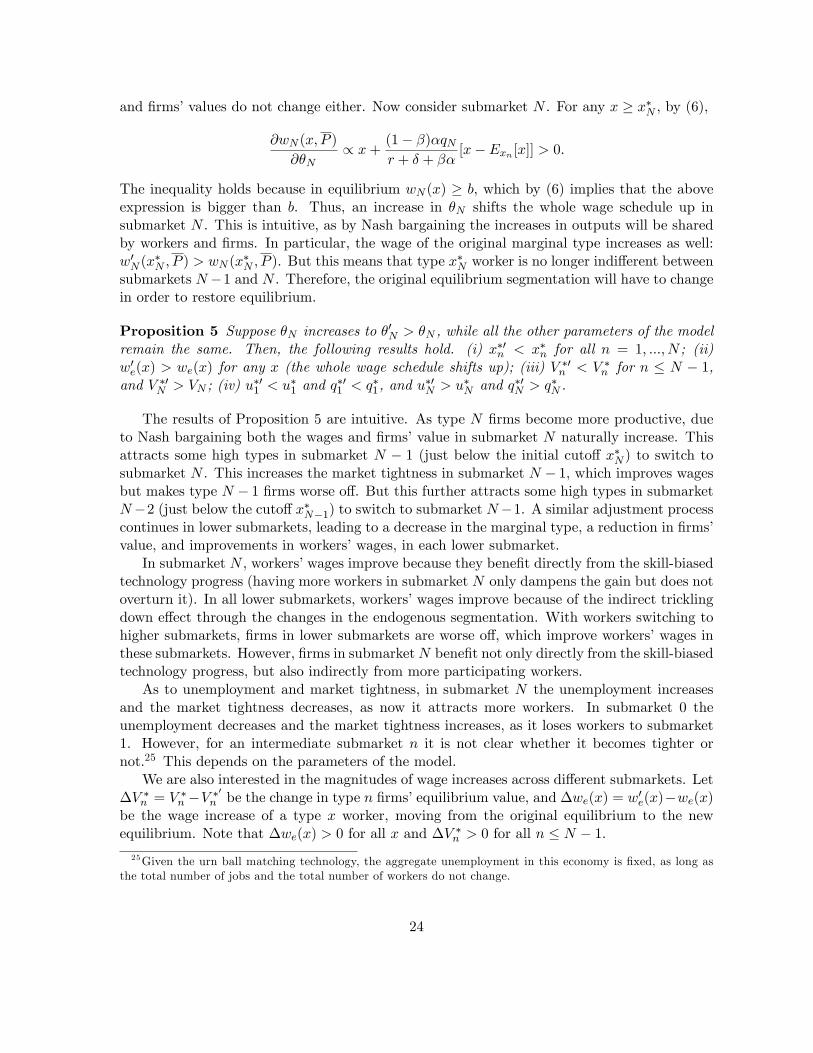
Proposition 6 For all x, the wage increase ∆we(x) is weakly increasing in x. In particular,(i) for all n ≤ N − 1, the decrease in firms’equilibrium value ∆V ∗n is increasing in n; (ii) forx ∈ [x∗n, x

∗′n+1], n ≤ N − 1, ∆we(x) is constant; (iii) for x ∈ [x∗′n+1, x

∗n+1], n ≤ N − 1, ∆we(x)

is strictly increasing in x; (iv) for x ≥ x∗′N , ∆we(x) is strictly increasing in x.

Proposition 6 implies that a skill-biased technology progress in the most productive submar-ket, though causing all wages to increase, increases wage inequality. In particular, it increaseswage inequality within each submarket (except for submarket 0). Within the most productivesubmarket N , wage becomes more unequal because an increase in θN , through Nash bargain-ing, makes the wage schedule steeper. Within submarket n, 1 ≤ n ≤ N , wage becomes moreunequal because the wage increases of the low switching types (x ∈ [x∗′n , x

∗n]) are smaller than

the wage increase of the high types (x ∈ [x∗n, x∗′n+1]), who do not switch submarkets. The

underlying reason for this pattern is that the low switching types suffer from an increase infirms’value as they switch to a higher submarket (V ∗n > V ∗n−1). Since the amount of wage in-creases becomes smaller in lower submarkets, the skill-biased technology progress also worsenswage inequality across submarkets. Using an analogy, since the initial positive shock happensin submarket N , the trickling down effect through the changes in endogenous segmentationtapers off in lower submarkets. which are further away from the source of the shock.

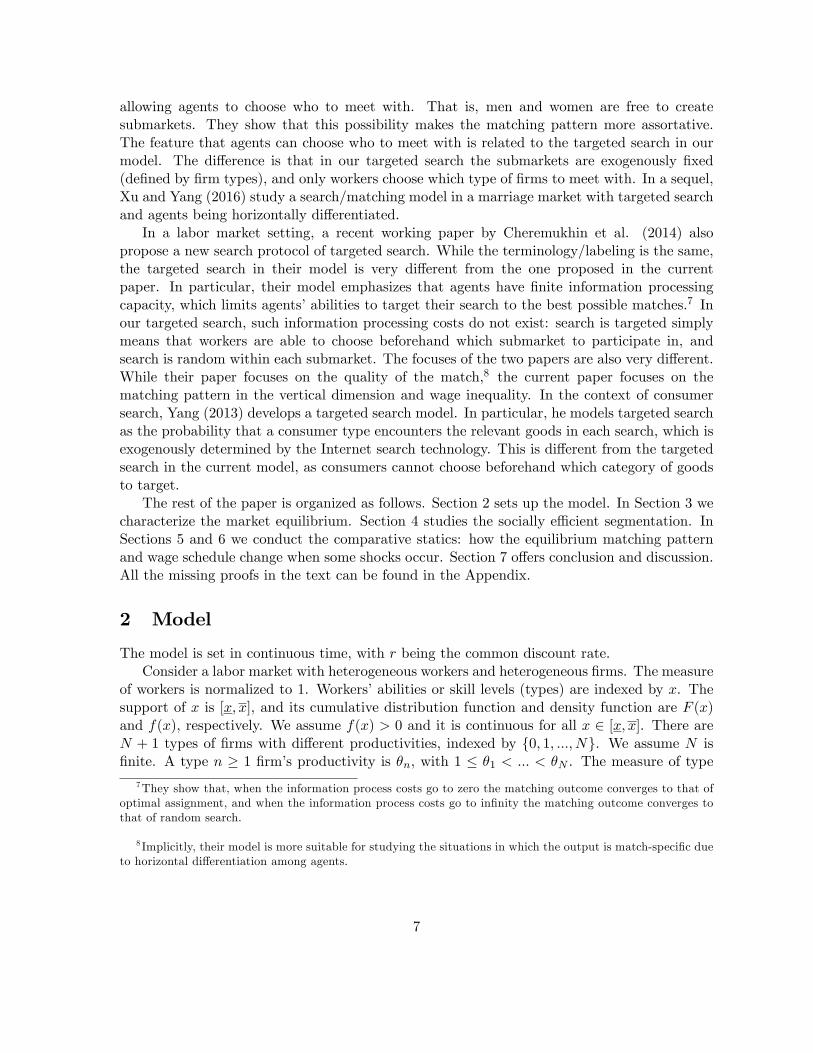
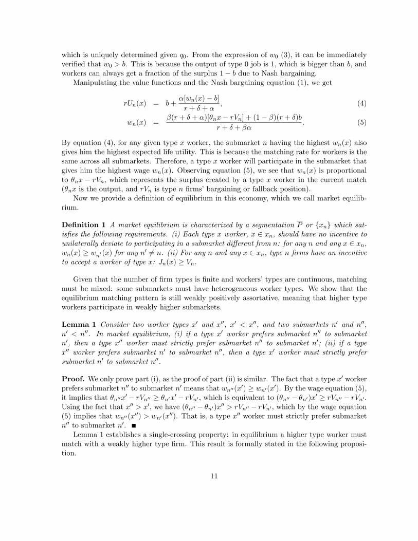
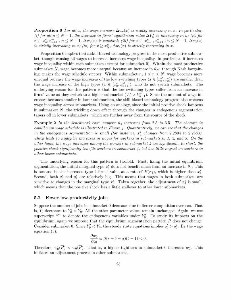
Example 2 In the benchmark case, suppose θ4 increases from 2.5 to 3.5. The changes inequilibrium wage schedule is illustrated in Figure 4. Quantitatively, we can see that the changesin the endogenous segmentation is small (for instance, x∗4 changes from 2.2894 to 2.2683),which leads to negligible increases in wages for workers in submarkets 0, 1, 2, and 3. On theother hand, the wage increases among the workers in submarket 4 are significant. In short, thepositive shock significantly benefits workers in submarket 4, but has little impact on workers inother lower submarkets.

The underlying reason for this pattern is twofold. First, fixing the initial equilibriumsegmentation, the initial marginal type x∗4 does not benefit much from an increase in θ4. Thisis because it also increases type 4 firms’value at a rate of E(x4), which is higher than x∗4.Second, both q∗3 and q

∗4 are relatively big. This means that wages in both submarkets are

sensitive to changes in the marginal type x∗4. Taken together, the adjustment of x∗4 is small,

which means that the positive shock has a little spillover to other lower submarkets.

5.2 Fewer low-productivity jobs

Suppose the number of jobs in submarket 0 decreases due to fiercer competition overseas. Thatis, Y0 decreases to Y ′0 < Y0. All the other parameter values remain unchanged. Again, we usesuperscript “′” to denote the endogenous variables under Y ′0 . To study its impacts on theequilibrium, again we suppose that the equilibrium segmentation pattern P does not change.Consider submarket 0. Since Y ′0 < Y0, the steady state equations implies q′0 > q∗0. By the wageequation (3),

∂w0

∂q0∝ β(r + δ + α)(b− 1) < 0.

Therefore, w′0(P ) < w0(P ). That is, a higher tightness in submarket 0 increases w0. Thisinitiates an adjustment process in other submarkets.

25

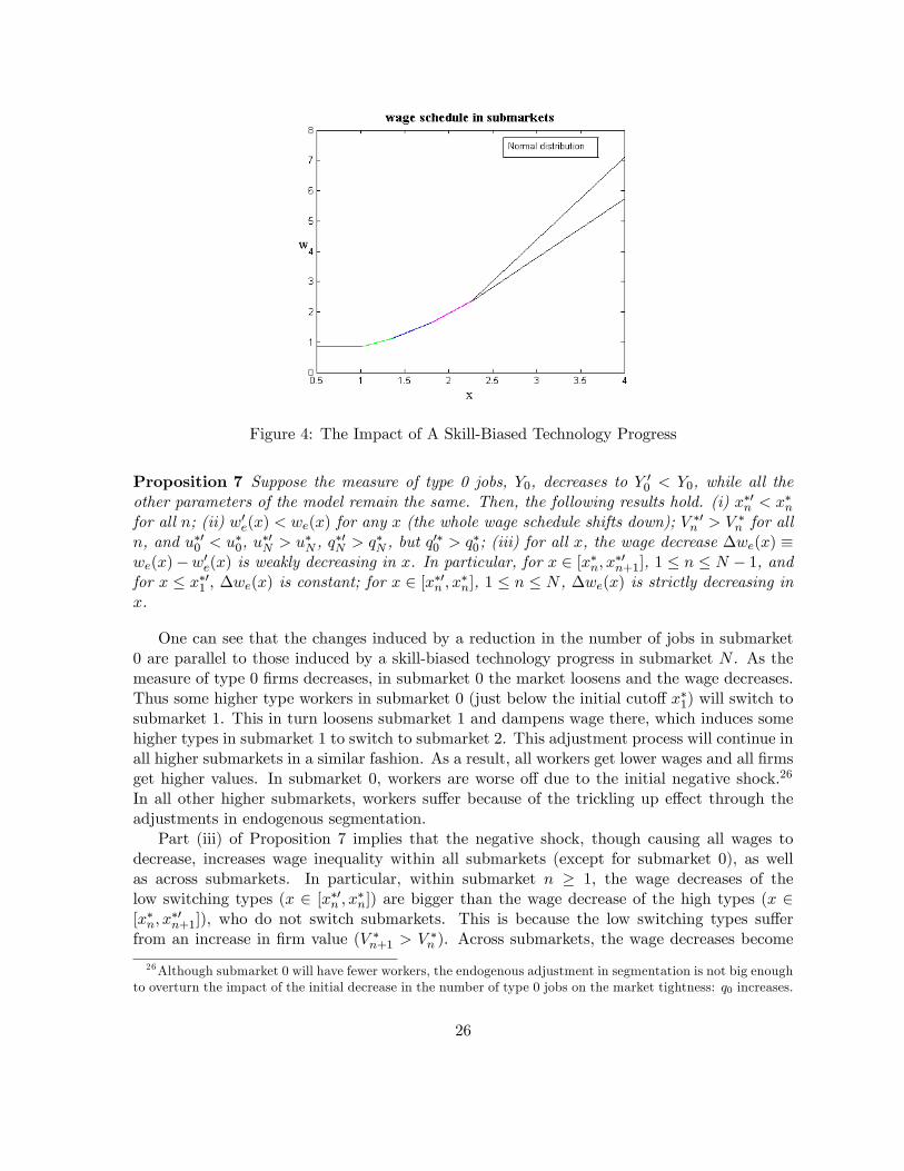
Figure 4: The Impact of A Skill-Biased Technology Progress

Proposition 7 Suppose the measure of type 0 jobs, Y0, decreases to Y ′0 < Y0, while all theother parameters of the model remain the same. Then, the following results hold. (i) x∗′n < x∗nfor all n; (ii) w′e(x) < we(x) for any x (the whole wage schedule shifts down); V ∗′n > V ∗n for alln, and u∗′0 < u∗0, u

∗′N > u∗N , q

∗′N > q∗N , but q

′∗0 > q∗0; (iii) for all x, the wage decrease ∆we(x) ≡

we(x)−w′e(x) is weakly decreasing in x. In particular, for x ∈ [x∗n, x∗′n+1], 1 ≤ n ≤ N − 1, and

for x ≤ x∗′1 , ∆we(x) is constant; for x ∈ [x∗′n , x∗n], 1 ≤ n ≤ N , ∆we(x) is strictly decreasing in

x.

One can see that the changes induced by a reduction in the number of jobs in submarket0 are parallel to those induced by a skill-biased technology progress in submarket N . As themeasure of type 0 firms decreases, in submarket 0 the market loosens and the wage decreases.Thus some higher type workers in submarket 0 (just below the initial cutoff x∗1) will switch tosubmarket 1. This in turn loosens submarket 1 and dampens wage there, which induces somehigher types in submarket 1 to switch to submarket 2. This adjustment process will continue inall higher submarkets in a similar fashion. As a result, all workers get lower wages and all firmsget higher values. In submarket 0, workers are worse off due to the initial negative shock.26

In all other higher submarkets, workers suffer because of the trickling up effect through theadjustments in endogenous segmentation.

Part (iii) of Proposition 7 implies that the negative shock, though causing all wages todecrease, increases wage inequality within all submarkets (except for submarket 0), as wellas across submarkets. In particular, within submarket n ≥ 1, the wage decreases of thelow switching types (x ∈ [x∗′n , x

∗n]) are bigger than the wage decrease of the high types (x ∈

[x∗n, x∗′n+1]), who do not switch submarkets. This is because the low switching types suffer

from an increase in firm value (V ∗n+1 > V ∗n ). Across submarkets, the wage decreases become

26Although submarket 0 will have fewer workers, the endogenous adjustment in segmentation is not big enoughto overturn the impact of the initial decrease in the number of type 0 jobs on the market tightness: q0 increases.

26

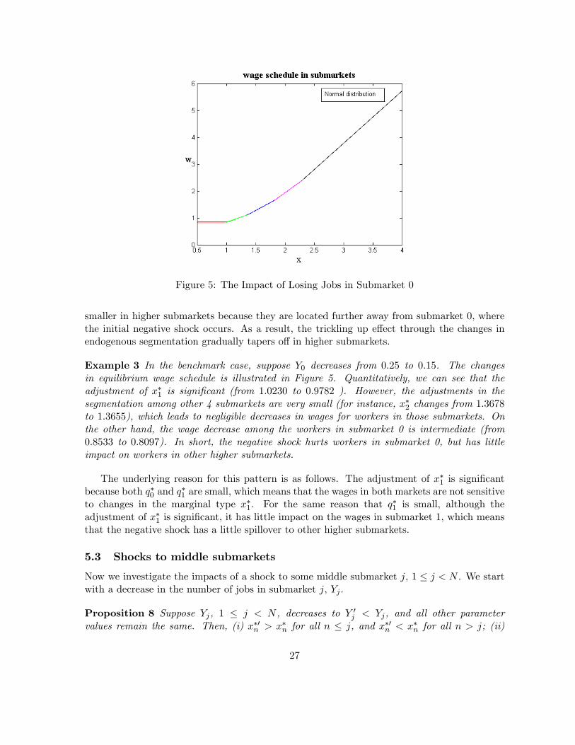
Figure 5: The Impact of Losing Jobs in Submarket 0

smaller in higher submarkets because they are located further away from submarket 0, wherethe initial negative shock occurs. As a result, the trickling up effect through the changes inendogenous segmentation gradually tapers off in higher submarkets.

Example 3 In the benchmark case, suppose Y0 decreases from 0.25 to 0.15. The changesin equilibrium wage schedule is illustrated in Figure 5. Quantitatively, we can see that theadjustment of x∗1 is significant (from 1.0230 to 0.9782 ). However, the adjustments in thesegmentation among other 4 submarkets are very small (for instance, x∗2 changes from 1.3678to 1.3655), which leads to negligible decreases in wages for workers in those submarkets. Onthe other hand, the wage decrease among the workers in submarket 0 is intermediate (from0.8533 to 0.8097). In short, the negative shock hurts workers in submarket 0, but has littleimpact on workers in other higher submarkets.

The underlying reason for this pattern is as follows. The adjustment of x∗1 is significantbecause both q∗0 and q

∗1 are small, which means that the wages in both markets are not sensitive

to changes in the marginal type x∗1. For the same reason that q∗1 is small, although theadjustment of x∗1 is significant, it has little impact on the wages in submarket 1, which meansthat the negative shock has a little spillover to other higher submarkets.

5.3 Shocks to middle submarkets

Now we investigate the impacts of a shock to some middle submarket j, 1 ≤ j < N . We startwith a decrease in the number of jobs in submarket j, Yj .

Proposition 8 Suppose Yj, 1 ≤ j < N , decreases to Y ′j < Yj, and all other parametervalues remain the same. Then, (i) x∗′n > x∗n for all n ≤ j, and x∗′n < x∗n for all n > j; (ii)

27

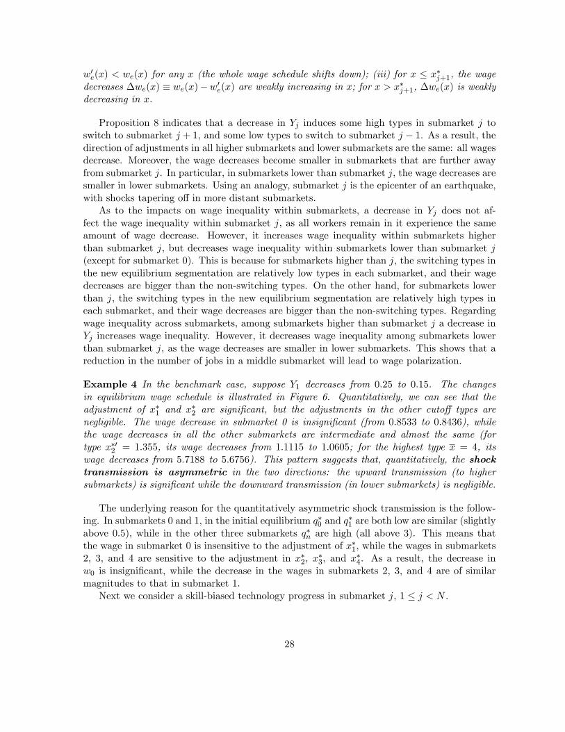
w′e(x) < we(x) for any x (the whole wage schedule shifts down); (iii) for x ≤ x∗j+1, the wagedecreases ∆we(x) ≡ we(x)−w′e(x) are weakly increasing in x; for x > x∗j+1, ∆we(x) is weaklydecreasing in x.

Proposition 8 indicates that a decrease in Yj induces some high types in submarket j toswitch to submarket j + 1, and some low types to switch to submarket j − 1. As a result, thedirection of adjustments in all higher submarkets and lower submarkets are the same: all wagesdecrease. Moreover, the wage decreases become smaller in submarkets that are further awayfrom submarket j. In particular, in submarkets lower than submarket j, the wage decreases aresmaller in lower submarkets. Using an analogy, submarket j is the epicenter of an earthquake,with shocks tapering off in more distant submarkets.

As to the impacts on wage inequality within submarkets, a decrease in Yj does not af-fect the wage inequality within submarket j, as all workers remain in it experience the sameamount of wage decrease. However, it increases wage inequality within submarkets higherthan submarket j, but decreases wage inequality within submarkets lower than submarket j(except for submarket 0). This is because for submarkets higher than j, the switching types inthe new equilibrium segmentation are relatively low types in each submarket, and their wagedecreases are bigger than the non-switching types. On the other hand, for submarkets lowerthan j, the switching types in the new equilibrium segmentation are relatively high types ineach submarket, and their wage decreases are bigger than the non-switching types. Regardingwage inequality across submarkets, among submarkets higher than submarket j a decrease inYj increases wage inequality. However, it decreases wage inequality among submarkets lowerthan submarket j, as the wage decreases are smaller in lower submarkets. This shows that areduction in the number of jobs in a middle submarket will lead to wage polarization.

Example 4 In the benchmark case, suppose Y1 decreases from 0.25 to 0.15. The changesin equilibrium wage schedule is illustrated in Figure 6. Quantitatively, we can see that theadjustment of x∗1 and x∗2 are significant, but the adjustments in the other cutoff types arenegligible. The wage decrease in submarket 0 is insignificant (from 0.8533 to 0.8436), whilethe wage decreases in all the other submarkets are intermediate and almost the same (fortype x∗′2 = 1.355, its wage decreases from 1.1115 to 1.0605; for the highest type x = 4, itswage decreases from 5.7188 to 5.6756). This pattern suggests that, quantitatively, the shocktransmission is asymmetric in the two directions: the upward transmission (to highersubmarkets) is significant while the downward transmission (in lower submarkets) is negligible.

The underlying reason for the quantitatively asymmetric shock transmission is the follow-ing. In submarkets 0 and 1, in the initial equilibrium q∗0 and q

∗1 are both low are similar (slightly

above 0.5), while in the other three submarkets q∗n are high (all above 3). This means thatthe wage in submarket 0 is insensitive to the adjustment of x∗1, while the wages in submarkets2, 3, and 4 are sensitive to the adjustment in x∗2, x

∗3, and x

∗4. As a result, the decrease in

w0 is insignificant, while the decrease in the wages in submarkets 2, 3, and 4 are of similarmagnitudes to that in submarket 1.

Next we consider a skill-biased technology progress in submarket j, 1 ≤ j < N .

28

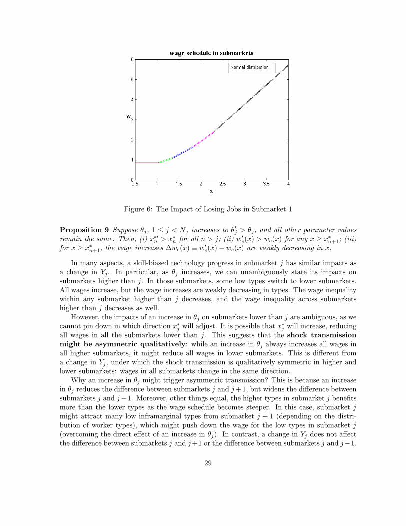
Figure 6: The Impact of Losing Jobs in Submarket 1

Proposition 9 Suppose θj, 1 ≤ j < N , increases to θ′j > θj, and all other parameter valuesremain the same. Then, (i) x∗′n > x∗n for all n > j; (ii) w′e(x) > we(x) for any x ≥ x∗n+1; (iii)for x ≥ x∗n+1, the wage increases ∆we(x) ≡ w′e(x)− we(x) are weakly decreasing in x.

In many aspects, a skill-biased technology progress in submarket j has similar impacts asa change in Yj . In particular, as θj increases, we can unambiguously state its impacts onsubmarkets higher than j. In those submarkets, some low types switch to lower submarkets.All wages increase, but the wage increases are weakly decreasing in types. The wage inequalitywithin any submarket higher than j decreases, and the wage inequality across submarketshigher than j decreases as well.

However, the impacts of an increase in θj on submarkets lower than j are ambiguous, as wecannot pin down in which direction x∗j will adjust. It is possible that x

∗j will increase, reducing

all wages in all the submarkets lower than j. This suggests that the shock transmissionmight be asymmetric qualitatively: while an increase in θj always increases all wages inall higher submarkets, it might reduce all wages in lower submarkets. This is different froma change in Yj , under which the shock transmission is qualitatively symmetric in higher andlower submarkets: wages in all submarkets change in the same direction.

Why an increase in θj might trigger asymmetric transmission? This is because an increasein θj reduces the difference between submarkets j and j+1, but widens the difference betweensubmarkets j and j−1. Moreover, other things equal, the higher types in submarket j benefitsmore than the lower types as the wage schedule becomes steeper. In this case, submarket jmight attract many low inframarginal types from submarket j + 1 (depending on the distri-bution of worker types), which might push down the wage for the low types in submarket j(overcoming the direct effect of an increase in θj). In contrast, a change in Yj does not affectthe difference between submarkets j and j+1 or the difference between submarkets j and j−1.

29

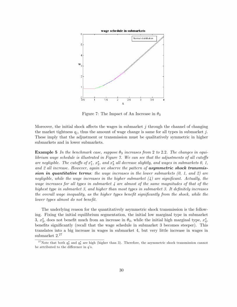
Figure 7: The Impact of An Increase in θ3

Moreover, the initial shock affects the wages in submarket j through the channel of changingthe market tightness qj , thus the amount of wage change is same for all types in submarket j.These imply that the adjustment or transmission must be qualitatively symmetric in highersubmarkets and in lower submarkets.

Example 5 In the benchmark case, suppose θ3 increases from 2 to 2.2. The changes in equi-librium wage schedule is illustrated in Figure 7. We can see that the adjustments of all cutoffsare negligible. The cutoffs of x∗1, x

∗2, and x

∗3 all decrease slightly, and wages in submarkets 0, 1,

and 2 all increase. However, again we observe the pattern of asymmetric shock transmis-sion in quantitative terms: the wage increases in the lower submarkets (0, 1, and 2) arenegligible, while the wage increases in the higher submarket (4) are significant. Actually, thewage increases for all types in submarket 4 are almost of the same magnitudes of that of thehighest type in submarket 3, and higher than most types in submarket 3. It definitely increasesthe overall wage inequality, as the higher types benefit significantly from the shock, while thelower types almost do not benefit.

The underlying reason for the quantitatively asymmetric shock transmission is the follow-ing. Fixing the initial equilibrium segmentation, the initial low marginal type in submarket3, x∗3, does not benefit much from an increase in θ3, while the initial high marginal type, x∗4,benefits significantly (recall that the wage schedule in submarket 3 becomes steeper). Thistranslates into a big increase in wages in submarket 4, but very little increase in wages insubmarket 2.27

27Note that both q∗2 and q∗4 are high (higher than 3). Therefore, the asymmetric shock transmission cannot

be attributed to the difference in q’s.

30

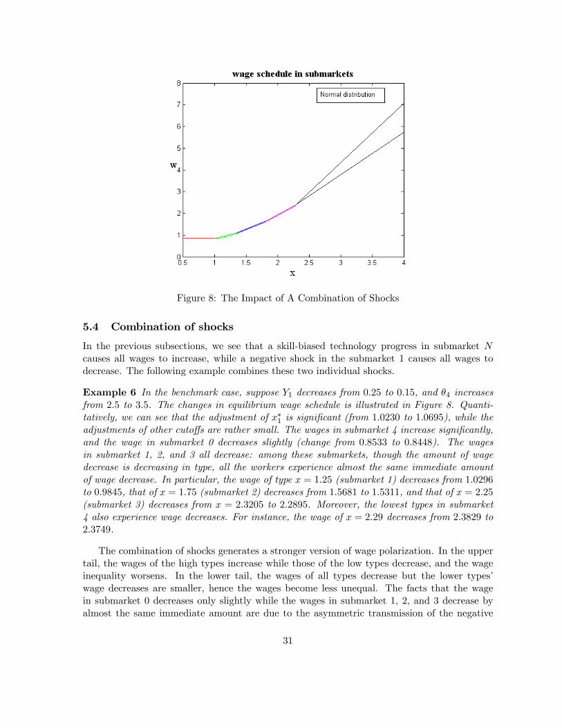
Figure 8: The Impact of A Combination of Shocks

5.4 Combination of shocks

In the previous subsections, we see that a skill-biased technology progress in submarket Ncauses all wages to increase, while a negative shock in the submarket 1 causes all wages todecrease. The following example combines these two individual shocks.

Example 6 In the benchmark case, suppose Y1 decreases from 0.25 to 0.15, and θ4 increasesfrom 2.5 to 3.5. The changes in equilibrium wage schedule is illustrated in Figure 8. Quanti-tatively, we can see that the adjustment of x∗1 is significant (from 1.0230 to 1.0695), while theadjustments of other cutoffs are rather small. The wages in submarket 4 increase significantly,and the wage in submarket 0 decreases slightly (change from 0.8533 to 0.8448). The wagesin submarket 1, 2, and 3 all decrease: among these submarkets, though the amount of wagedecrease is decreasing in type, all the workers experience almost the same immediate amountof wage decrease. In particular, the wage of type x = 1.25 (submarket 1) decreases from 1.0296to 0.9845, that of x = 1.75 (submarket 2) decreases from 1.5681 to 1.5311, and that of x = 2.25(submarket 3) decreases from x = 2.3205 to 2.2895. Moreover, the lowest types in submarket4 also experience wage decreases. For instance, the wage of x = 2.29 decreases from 2.3829 to2.3749.

The combination of shocks generates a stronger version of wage polarization. In the uppertail, the wages of the high types increase while those of the low types decrease, and the wageinequality worsens. In the lower tail, the wages of all types decrease but the lower types’wage decreases are smaller, hence the wages become less unequal. The facts that the wagein submarket 0 decreases only slightly while the wages in submarket 1, 2, and 3 decrease byalmost the same immediate amount are due to the asymmetric transmission of the negative

31

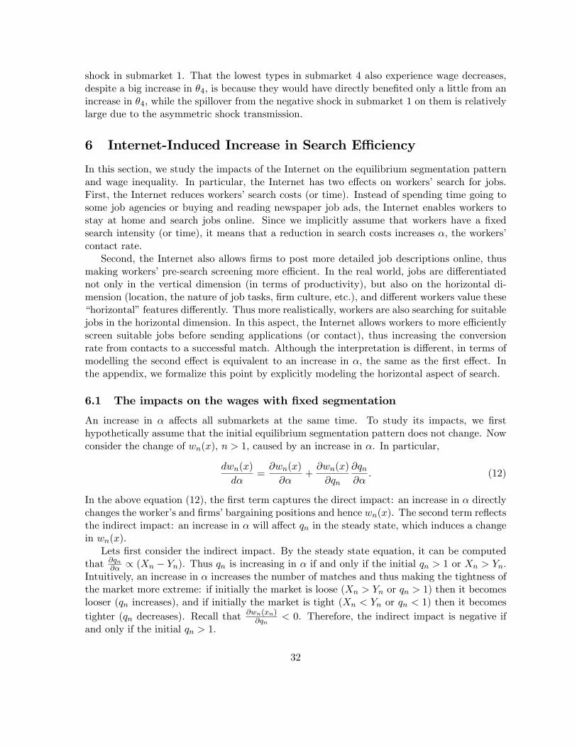
shock in submarket 1. That the lowest types in submarket 4 also experience wage decreases,despite a big increase in θ4, is because they would have directly benefited only a little from anincrease in θ4, while the spillover from the negative shock in submarket 1 on them is relativelylarge due to the asymmetric shock transmission.

6 Internet-Induced Increase in Search Effi ciency

In this section, we study the impacts of the Internet on the equilibrium segmentation patternand wage inequality. In particular, the Internet has two effects on workers’ search for jobs.First, the Internet reduces workers’search costs (or time). Instead of spending time going tosome job agencies or buying and reading newspaper job ads, the Internet enables workers tostay at home and search jobs online. Since we implicitly assume that workers have a fixedsearch intensity (or time), it means that a reduction in search costs increases α, the workers’contact rate.

Second, the Internet also allows firms to post more detailed job descriptions online, thusmaking workers’pre-search screening more effi cient. In the real world, jobs are differentiatednot only in the vertical dimension (in terms of productivity), but also on the horizontal di-mension (location, the nature of job tasks, firm culture, etc.), and different workers value these“horizontal”features differently. Thus more realistically, workers are also searching for suitablejobs in the horizontal dimension. In this aspect, the Internet allows workers to more effi cientlyscreen suitable jobs before sending applications (or contact), thus increasing the conversionrate from contacts to a successful match. Although the interpretation is different, in terms ofmodelling the second effect is equivalent to an increase in α, the same as the first effect. Inthe appendix, we formalize this point by explicitly modeling the horizontal aspect of search.

6.1 The impacts on the wages with fixed segmentation

An increase in α affects all submarkets at the same time. To study its impacts, we firsthypothetically assume that the initial equilibrium segmentation pattern does not change. Nowconsider the change of wn(x), n > 1, caused by an increase in α. In particular,

dwn(x)

dα=∂wn(x)

∂α+∂wn(x)

∂qn

∂qn∂α

. (12)

In the above equation (12), the first term captures the direct impact: an increase in α directlychanges the worker’s and firms’bargaining positions and hence wn(x). The second term reflectsthe indirect impact: an increase in α will affect qn in the steady state, which induces a changein wn(x).

Lets first consider the indirect impact. By the steady state equation, it can be computedthat ∂qn

∂α ∝ (Xn − Yn). Thus qn is increasing in α if and only if the initial qn > 1 or Xn > Yn.Intuitively, an increase in α increases the number of matches and thus making the tightness ofthe market more extreme: if initially the market is loose (Xn > Yn or qn > 1) then it becomeslooser (qn increases), and if initially the market is tight (Xn < Yn or qn < 1) then it becomestighter (qn decreases). Recall that

∂wn(xn)∂qn

< 0. Therefore, the indirect impact is negative ifand only if the initial qn > 1.

32

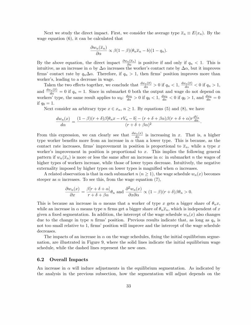
Next we study the direct impact. First, we consider the average type xn ≡ E(xn). By thewage equation (6), it can be calculated that

∂wn(xn)

∂α∝ β(1− β)(θnxn − b)(1− qn).

By the above equation, the direct impact ∂wn(xn)∂α is positive if and only if qn < 1. This is

intuitive, as an increase in α by ∆α increases the worker’s contact rate by ∆α, but it improvesfirms’contact rate by qn∆α. Therefore, if qn > 1, then firms’position improves more thanworker’s, leading to a decrease in wage.

Taken the two effects together, we conclude that dwn(x)dα > 0 if qn < 1, dwn(x)

dα < 0 if qn > 1,

and dwn(x)dα = 0 if qn = 1. Since in submarket 0 both the output and wage do not depend on

workers’type, the same result applies to w0: dw0dα > 0 if q0 < 1, dw0dα < 0 if q0 > 1, and dw0

dα = 0if q0 = 1.

Next consider an arbitrary type x ∈ xn, n ≥ 1. By equations (5) and (8), we have

dwn(x)

dα=

(1− β)(r + δ)β[θnx− rVn − b]− (r + δ + βα)β(r + δ + α)r dVndα(r + δ + βα)2

.

From this expression, we can clearly see that dwn(x)dα is increasing in x. That is, a higher

type worker benefits more from an increase in α than a lower type. This is because, as thecontact rate increases, firms’ improvement in position is proportional to xn, while a type xworker’s improvement in position is proportional to x. This implies the following generalpattern if wn(xn) is more or less the same after an increase in α: in submarket n the wages ofhigher types of workers increase, while those of lower types decrease. Intuitively, the negativeexternality imposed by higher types on lower types is magnified when α increases.

A related observation is that in each submarket n (n ≥ 1), the wage schedule wn(x) becomessteeper as α increases. To see this, from the wage equation (7),

∂wn(x)

∂x=β[r + δ + α]

r + δ + βαθn and

∂2wn(x)

∂x∂α∝ (1− β)(r + δ)βθn > 0.

This is because an increase in α means that a worker of type x gets a bigger share of θnx,while an increase in α means type n firms get a bigger share of θnxn, which is independent of xgiven a fixed segmentation. In addition, the intercept of the wage schedule wn(x) also changesdue to the change in type n firms’position. Previous results indicate that, as long as qn isnot too small relative to 1, firms’position will improve and the intercept of the wage scheduledecreases.

The impacts of an increase in α on the wage schedules, fixing the initial equilibrium segme-nation, are illustrated in Figure 9, where the solid lines indicate the initial equilibrium wageschedule, while the dashed lines represent the new ones.

6.2 Overall Impacts

An increase in α will induce adjustments in the equilibrium segmentation. As indicated bythe analysis in the previous subsection, how the segmentation will adjust depends on the

33

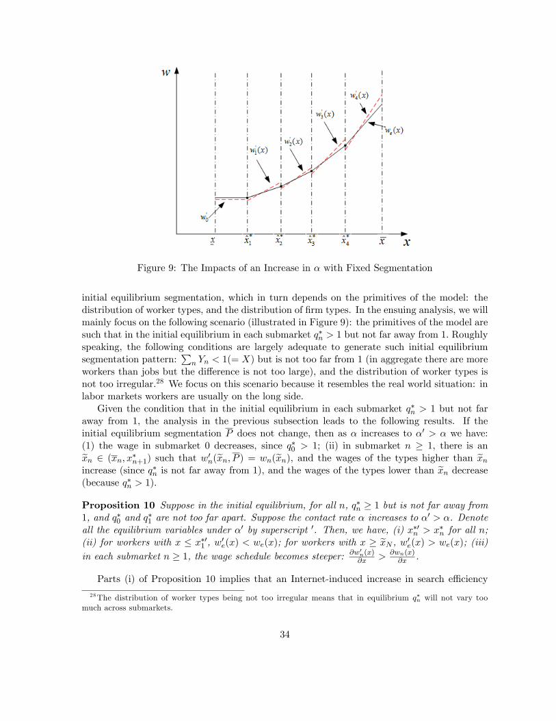
Figure 9: The Impacts of an Increase in α with Fixed Segmentation

initial equilibrium segmentation, which in turn depends on the primitives of the model: thedistribution of worker types, and the distribution of firm types. In the ensuing analysis, we willmainly focus on the following scenario (illustrated in Figure 9): the primitives of the model aresuch that in the initial equilibrium in each submarket q∗n > 1 but not far away from 1. Roughlyspeaking, the following conditions are largely adequate to generate such initial equilibriumsegmentation pattern:

∑n Yn < 1(= X) but is not too far from 1 (in aggregate there are more

workers than jobs but the difference is not too large), and the distribution of worker types isnot too irregular.28 We focus on this scenario because it resembles the real world situation: inlabor markets workers are usually on the long side.

Given the condition that in the initial equilibrium in each submarket q∗n > 1 but not faraway from 1, the analysis in the previous subsection leads to the following results. If theinitial equilibrium segmentation P does not change, then as α increases to α′ > α we have:(1) the wage in submarket 0 decreases, since q∗0 > 1; (ii) in submarket n ≥ 1, there is anxn ∈ (xn, x

∗n+1) such that w′n(xn, P ) = wn(xn), and the wages of the types higher than xn

increase (since q∗n is not far away from 1), and the wages of the types lower than xn decrease(because q∗n > 1).

Proposition 10 Suppose in the initial equilibrium, for all n, q∗n ≥ 1 but is not far away from1, and q∗0 and q

∗1 are not too far apart. Suppose the contact rate α increases to α

′ > α. Denoteall the equilibrium variables under α′ by superscript ′. Then, we have, (i) x∗′n > x∗n for all n;(ii) for workers with x ≤ x∗′1 , w

′e(x) < we(x); for workers with x ≥ xN , w′e(x) > we(x); (iii)

in each submarket n ≥ 1, the wage schedule becomes steeper: ∂w′n(x)∂x > ∂wn(x)

∂x .

Parts (i) of Proposition 10 implies that an Internet-induced increase in search effi ciency

28The distribution of worker types being not too irregular means that in equilibrium q∗n will not vary toomuch across submarkets.

34

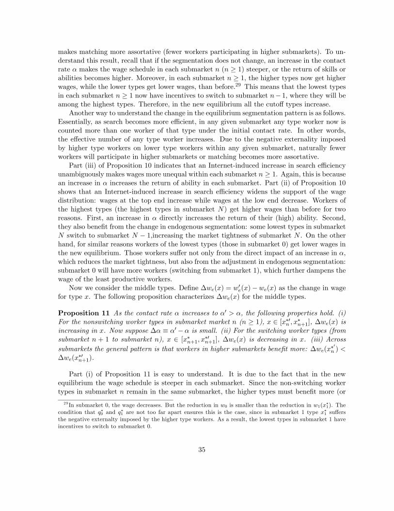
makes matching more assortative (fewer workers participating in higher submarkets). To un-derstand this result, recall that if the segmentation does not change, an increase in the contactrate α makes the wage schedule in each submarket n (n ≥ 1) steeper, or the return of skills orabilities becomes higher. Moreover, in each submarket n ≥ 1, the higher types now get higherwages, while the lower types get lower wages, than before.29 This means that the lowest typesin each submarket n ≥ 1 now have incentives to switch to submarket n− 1, where they will beamong the highest types. Therefore, in the new equilibrium all the cutoff types increase.

Another way to understand the change in the equilibrium segmentation pattern is as follows.Essentially, as search becomes more effi cient, in any given submarket any type worker now iscounted more than one worker of that type under the initial contact rate. In other words,the effective number of any type worker increases. Due to the negative externality imposedby higher type workers on lower type workers within any given submarket, naturally fewerworkers will participate in higher submarkets or matching becomes more assortative.

Part (iii) of Proposition 10 indicates that an Internet-induced increase in search effi ciencyunambiguously makes wages more unequal within each submarket n ≥ 1. Again, this is becausean increase in α increases the return of ability in each submarket. Part (ii) of Proposition 10shows that an Internet-induced increase in search effi ciency widens the support of the wagedistribution: wages at the top end increase while wages at the low end decrease. Workers ofthe highest types (the highest types in submarket N) get higher wages than before for tworeasons. First, an increase in α directly increases the return of their (high) ability. Second,they also benefit from the change in endogenous segmentation: some lowest types in submarketN switch to submarket N − 1,increasing the market tightness of submarket N . On the otherhand, for similar reasons workers of the lowest types (those in submarket 0) get lower wages inthe new equilibrium. Those workers suffer not only from the direct impact of an increase in α,which reduces the market tightness, but also from the adjustment in endogenous segmentation:submarket 0 will have more workers (switching from submarket 1), which further dampens thewage of the least productive workers.

Now we consider the middle types. Define ∆we(x) = w′e(x)−we(x) as the change in wagefor type x. The following proposition characterizes ∆we(x) for the middle types.

Proposition 11 As the contact rate α increases to α′ > α, the following properties hold. (i)For the nonswitching worker types in submarket market n (n ≥ 1), x ∈ [x∗′n , x

∗n+1], ∆we(x) is

increasing in x. Now suppose ∆α ≡ α′ −α is small. (ii) For the switching worker types (fromsubmarket n + 1 to submarket n), x ∈ [x∗n+1, x

∗′n+1], ∆we(x) is decreasing in x. (iii) Across

submarkets the general pattern is that workers in higher submarkets benefit more: ∆we(x∗′n ) <

∆we(x∗′n+1).

Part (i) of Proposition 11 is easy to understand. It is due to the fact that in the newequilibrium the wage schedule is steeper in each submarket. Since the non-switching workertypes in submarket n remain in the same submarket, the higher types must benefit more (or

29 In submarket 0, the wage decreases. But the reduction in w0 is smaller than the reduction in w1(x∗1). Thecondition that q∗0 and q

∗1 are not too far apart ensures this is the case, since in submarket 1 type x

∗1 suffers

the negative externalty imposed by the higher type workers. As a result, the lowest types in submarket 1 haveincentives to switch to submarket 0.

35

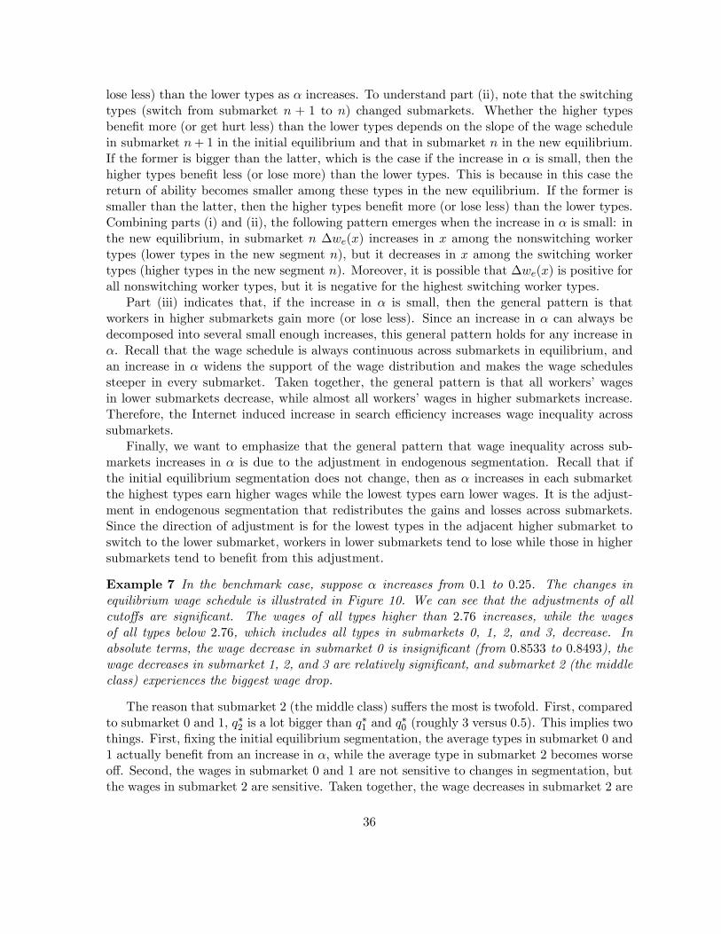
lose less) than the lower types as α increases. To understand part (ii), note that the switchingtypes (switch from submarket n + 1 to n) changed submarkets. Whether the higher typesbenefit more (or get hurt less) than the lower types depends on the slope of the wage schedulein submarket n+ 1 in the initial equilibrium and that in submarket n in the new equilibrium.If the former is bigger than the latter, which is the case if the increase in α is small, then thehigher types benefit less (or lose more) than the lower types. This is because in this case thereturn of ability becomes smaller among these types in the new equilibrium. If the former issmaller than the latter, then the higher types benefit more (or lose less) than the lower types.Combining parts (i) and (ii), the following pattern emerges when the increase in α is small: inthe new equilibrium, in submarket n ∆we(x) increases in x among the nonswitching workertypes (lower types in the new segment n), but it decreases in x among the switching workertypes (higher types in the new segment n). Moreover, it is possible that ∆we(x) is positive forall nonswitching worker types, but it is negative for the highest switching worker types.

Part (iii) indicates that, if the increase in α is small, then the general pattern is thatworkers in higher submarkets gain more (or lose less). Since an increase in α can always bedecomposed into several small enough increases, this general pattern holds for any increase inα. Recall that the wage schedule is always continuous across submarkets in equilibrium, andan increase in α widens the support of the wage distribution and makes the wage schedulessteeper in every submarket. Taken together, the general pattern is that all workers’wagesin lower submarkets decrease, while almost all workers’wages in higher submarkets increase.Therefore, the Internet induced increase in search effi ciency increases wage inequality acrosssubmarkets.

Finally, we want to emphasize that the general pattern that wage inequality across sub-markets increases in α is due to the adjustment in endogenous segmentation. Recall that ifthe initial equilibrium segmentation does not change, then as α increases in each submarketthe highest types earn higher wages while the lowest types earn lower wages. It is the adjust-ment in endogenous segmentation that redistributes the gains and losses across submarkets.Since the direction of adjustment is for the lowest types in the adjacent higher submarket toswitch to the lower submarket, workers in lower submarkets tend to lose while those in highersubmarkets tend to benefit from this adjustment.

Example 7 In the benchmark case, suppose α increases from 0.1 to 0.25. The changes inequilibrium wage schedule is illustrated in Figure 10. We can see that the adjustments of allcutoffs are significant. The wages of all types higher than 2.76 increases, while the wagesof all types below 2.76, which includes all types in submarkets 0, 1, 2, and 3, decrease. Inabsolute terms, the wage decrease in submarket 0 is insignificant (from 0.8533 to 0.8493), thewage decreases in submarket 1, 2, and 3 are relatively significant, and submarket 2 (the middleclass) experiences the biggest wage drop.

The reason that submarket 2 (the middle class) suffers the most is twofold. First, comparedto submarket 0 and 1, q∗2 is a lot bigger than q

∗1 and q

∗0 (roughly 3 versus 0.5). This implies two

things. First, fixing the initial equilibrium segmentation, the average types in submarket 0 and1 actually benefit from an increase in α, while the average type in submarket 2 becomes worseoff. Second, the wages in submarket 0 and 1 are not sensitive to changes in segmentation, butthe wages in submarket 2 are sensitive. Taken together, the wage decreases in submarket 2 are

36

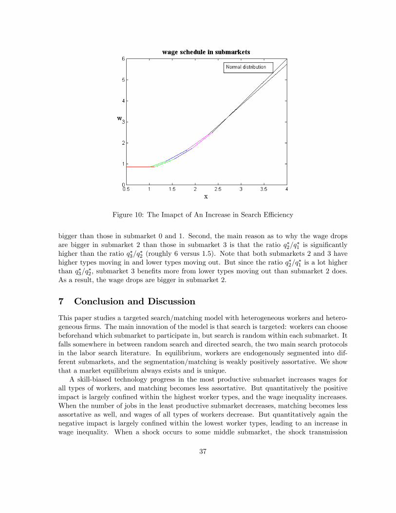
Figure 10: The Imapct of An Increase in Search Effi ciency

bigger than those in submarket 0 and 1. Second, the main reason as to why the wage dropsare bigger in submarket 2 than those in submarket 3 is that the ratio q∗2/q

∗1 is significantly

higher than the ratio q∗3/q∗2 (roughly 6 versus 1.5). Note that both submarkets 2 and 3 have

higher types moving in and lower types moving out. But since the ratio q∗2/q∗1 is a lot higher

than q∗3/q∗2, submarket 3 benefits more from lower types moving out than submarket 2 does.

As a result, the wage drops are bigger in submarket 2.

7 Conclusion and Discussion

This paper studies a targeted search/matching model with heterogeneous workers and hetero-geneous firms. The main innovation of the model is that search is targeted: workers can choosebeforehand which submarket to participate in, but search is random within each submarket. Itfalls somewhere in between random search and directed search, the two main search protocolsin the labor search literature. In equilibrium, workers are endogenously segmented into dif-ferent submarkets, and the segmentation/matching is weakly positively assortative. We showthat a market equilibrium always exists and is unique.

A skill-biased technology progress in the most productive submarket increases wages forall types of workers, and matching becomes less assortative. But quantitatively the positiveimpact is largely confined within the highest worker types, and the wage inequality increases.When the number of jobs in the least productive submarket decreases, matching becomes lessassortative as well, and wages of all types of workers decrease. But quantitatively again thenegative impact is largely confined within the lowest worker types, leading to an increase inwage inequality. When a shock occurs to some middle submarket, the shock transmission

37

quantitatively exhibits asymmetry: the wages in the higher submarkets are affected more thanthe wages in the lower submarkets. When the productivity of some middle submarket increases,the shock transmission might exhibit qualitative asymmetry: wages in the higher submarketsalways increase but wages in the lower submarkets might decrease.

The widespread use of the Internet in the last two decades indeed could have contributedto the rising wage inequality. When an Internet-induced increase in search effi ciency occurs,matching becomes more assortative, the wage schedule in each submarket becomes steeper, andthe wages of the highest types increase while those of the lowest types decrease. Therefore, itnot only increases the wage inequality among workers having similar jobs, but also increasesthe overall wage inequality across all types of workers.

In the rest of this section, we discuss how the main results of our model will change whenwe relax some of the assumptions.

Free entry In the model we have assumed that the number of jobs in each submarket is fixedand exogenously given. Here we briefly discuss how to incorporate free entry and endogenizethe number of jobs. Like Moen (1997), we assume that firms are ex ante homogeneous beforeentry. If a firm decides to enter, then it pays a sunk cost of entry and draws a productivitytype according to an exogenously fixed probability distribution. Thus the number of jobs in aparticular submarket is always a fixed fraction of the total number of jobs. The only differenceis that the total number of jobs is now endogenously determined by free entry: a firm’s ex anteexpected gross profit of entering must equal to the entry cost.

The existence and uniqueness of the equilibrium, as well as the equilibrium properties, willnot be qualitatively affected by free entry, as it just adds a free entry condition to determine thetotal number of jobs. Free entry would certainly complicate the comparative statics analysis.For instance, a skill-biased technology progress in some high submarket would also induce anadjustment in the total number of jobs. However, we expect all the comparative statics resultsto hold qualitatively even with free entry. This is because the induced adjustment in the totalnumber of jobs will be relatively small in magnitude, and it will not overturn the pattern of theimpacts of the shock on different submarkets without free entry. The underlying reason is thatthe free entry condition only determines the total number of jobs, but not the fraction of jobsin each submarket. As a result, the comparison across submarkets will not be qualitativelyaffected by free entry. For instance, when a skill-biased technology progress occurs in themost productive submarket, firms’ value in each submarket increases, thus more firms willenter. This further increases workers’wages. However, it will not qualitatively change thecomparison of wages across submarkets, as the fraction of jobs in each submarket is always thesame.

Urn ball matching technology The urn ball matching technology greatly simplifies ouranalysis. In particular, it means that a worker’s contact rate in any submarket, regardless ofthe worker’s type and the market tightness, is always fixed. It further implies that a worker’sexpected waiting time before getting employed in any submarket is always the same. As aresult, each worker will choose the submarket which gives him the highest wage. With a moregeneral matching technology, a worker’s contact rate in submarket n will negatively depend onqn, the expected queue length. It implies that a worker’s expected waiting time before getting

38

employed in submarket n is increasing in qn. As a result, figuring out which submarket a workerwill choose to participate in becomes hard, as his lifetime discounted utility depends on boththe wage and the expected waiting time. In a nutshell, a more general matching technologyintroduces coordination/congestion friction among workers (they impose direct externalitiesamong each other through the contact rate), which is absent under the urn ball matching tech-nology. However, we believe that having coordination/congestion friction will not qualitativelyaffect our main results. This is because the direct externality due to the congestion frictionworks in the same direction as the indirect externality that has been captured in our model:a larger qn increases firms’ contact rate and hence their continuation value, which throughNash bargaining reduces workers’wages and the attractiveness of submarket n to workers.Quantitatively, introducing the direct congestion externality would reduce the differences of qnacross submarkets in the equilibrium, as the impact of qn is magnified.

The finiteness of firm types This is mainly a modeling device, which ensures the num-ber of submarkets is finite. Moreover, it also implies that within each submarket there willbe workers of different abilities, under which random search within the submarkets becomessensible. In some sense, this assumption is also realistic, as anecdotally the labor market isvertically segmented into a finite number of sectors. To approximate the case that firm typesare continuous, we can increase the number of firm types N and let it approaches infinity.

39

Appendix

Proof of Lemma 3.Proof. We first show that, for all n ≥ 1, wn(x∗n) ≥ w0 > b. To see this, note that w1(x∗1) = w0

by the indifference condition (10). Since wn(x) is increasing in x, we have w2(x∗2) = w1(x∗2) >w1(x∗1) = w0. By induction, for all n ≥ 1 we have wn(x∗n) > w0 > b.

Next we show that, for any n ≥ 1, Jn(x∗n) > Vn if type n firms accept all workers withx ∈ (x∗n, x

∗n+1]. Since Jn(x) is increasing in x, this property also implies that Jn(x) > Vn for

any x ∈ [x∗n, x∗n+1]. To see that Jn(x∗n) > Vn, inspect equation (9). Since wn(x∗n) > b, equation

(9) implies that Jn(x∗n) > Vn.Finally, we rule out the possibility that a type n firm can increase its Vn by accepting

only a strict subset of workers. Since Jn(x) is increasing, we only need to worry about a firmaccepting higher types but rejecting lower types. Suppose a type n firm unilaterally deviatesto only accepting workers whose types are within [xn, x

∗n+1], xn ∈ (x∗n, x

∗n+1), and rejecting all

types below xn. Note that this individual deviation will not affect the market wage schedule,wn(x), as it is pinned down by the market conditions. Denote Vn as a type n firm’valuedeviating to this strategy. And Jn(x) and qn < qn are defined accordingly.30 Suppose there isa xn such that Vn > Vn. Using the value functions of Vn and Jn(x), we can express the valueof Vn as

rVn =αqnEx∈[xn,x∗n+1][θnx− wn(x)]

r + δ + αqn. (13)

The value function of Vn can also be written as

rVn = αqn[Ex∈[xn,x∗n+1](Jn(x))− Vn] + α(qn − qn)[Ex∈[x∗n,xn](Jn(x))− Vn].

Using the value function of Jn(x), we can express Vn as

rVn =αqnEx∈[xn,x∗n+1][θnx− wn(x)]

r + δ + αqn+ α(qn − qn)[Ex∈[x∗n,xn](Jn(x))− Vn]. (14)

By the expressions of (13) and (14), Vn > Vn implies that Ex∈[x∗n,xn](Jn(x)) − Vn < 0. SinceJn(x∗n) < Ex∈[x∗n,xn](Jn(x)), we have Jn(x∗n) < Vn, a contradiction. Therefore, there is noxn ∈ (x∗n, x

∗n+1) such that an individual type n firm can increase its Vn by accepting only

worker types above type xn.

Proof of Lemma 4.Proof. Part (i). By (5), it is immediate that w′n(x′) > w′′n(x′) if and only if V ′n < V ′′n .

Part (ii). As x1 increases, the measure of workers active in submarket 0, X0, increases. Itfollows from the steady-state equation that q0 increases. By part (i) of Lemma 2, ∂w0∂q0

< 0.Thus, w0 is strictly decreasing in x1. By part (i), it follows that V0 is strictly increasing in x1.

Part (iii). Suppose xN decreases to x′N < xN . The measure of workers active in submarketN , XN , increases. It follows from the steady-state equation that qN increases to q′N . For thecorresponding VN and V ′N , we must have V

′N ≥ VN . This is because type N firms can always

30Specifically, qn = qnF (x∗n+1)−F (xn)F (x∗n+1)−F (x∗n)

.

40

accept only the original set of workers x ≥ xN , which guarantees V ′N ≥ VN . If type N firmshave incentives to accept type x′N , then V

′N ≥ θN x′N + b. By an argument similar to the proof

of Lemma 3, it implies that V ′N > VN .Part (iv). Given that [xn, xn+1] v [x′n, x

′n+1], V ′N ≥ VN follows immediately since type n

firms can always accept only the original set of workers [xn, xn+1]. Now suppose xn+1 < x′n+1

and x′n ≤ xn. With the set of participating workers’types being x′n, type n firms can alwaysaccept only the higher type workers and rejecting the lower types such that the measure ofaccepted workers X ′n = Xn, and thus q′n = qn. Since xn+1 < x′n+1, the new accepted set ofworkers are on average more productive than the original set. By equation (8), V ′N > VN . Nowconsider the case that xn+1 ≤ x′n+1 and x

′n < xn and firms accept type x′n workers. This is

case is isomorphic to the proof in part (iii), thus a similar argument follows.

Proof of Lemma 6.Proof. Since the results of Lemma 5 apply to i = n− 1, given xn+1 we only need to focus onxn, or the segmentation between submarket n and the rest of the lower submarkets, and theequilibrium indifference condition between submarkets n − 1 and n. Denote a segmentationwith xn and the corresponding {x∗i }n−1

i=1 induced by xn as P (xn). From the wage equation (6),we can compute wn(xn;P (xn)) and wn−1(xn;P (xn)), which define two wage schedules as afunction of xn. Note that both wage schedules are continuous in xn. Again, possibly there aretwo kinds of equilibria, with the equilibrium conditions explicitly listed below:

Corner equilibrium: x∗n = x if wn(x;P (x)) ≥ wn−1(x),

Interior Equilibrium: x∗n ∈ (x, xn+1) if there is an xn such that wn(xn;P (xn)) = wn−1(xn;P (xn)).

Now we examine the properties of the wage schedules wn(xn;P (xn)) and wn−1(xn;P (xn)).As to wn(xn;P (xn)), wn = wn(x;P (x)) when xn = x, it monotonically increases as xn in-creases, and it reaches wn(xn+1) when xn = xn+1. Note that the monotonicity follows Lemma4: as xn increases fewer workers are active in submarket n and thus all wages in this submarketmust increase. Regarding wn−1(xn;P (xn)), it starts at wn−1(x) when xn = x, and it reaches atwn−1(xn+1;P (xn+1)) when xn = xn+1. We do not know whether wn−1(xn;P (xn)) is increasingor decreasing in xn, as there are two opposite effects.

Existence. We first show that an equilibrium x∗n must exist. To show this, consider twopossible cases. Case 1: suppose wn(x;P (x)) ≥ wn−1(x). Then by the equilibrium condition,the unique equilibrium is a corner equilibrium x∗n = x, with all workers participating in sub-market n. Case 2: wn(x;P (x)) < wn−1(x). In this case, the corner equilibrium does notexist. However, an interior equilibrium exists. To see this, note that wn−1(xn+1;P (xn+1)) ≤wn−1(xn+1) < wn(xn+1). Combining with the condition that wn(x;P (x)) < wn−1(x), we havethat, in the domain of [x, xn+1], the wage schedule wn−1(xn;P (xn)) starts above the wageschedule wn(xn;P (xn)), but it ends up below wn(xn;P (xn)). Since both wage schedules arecontinuous in xn, they must have an interior intersection, which is an interior equilibrium.This completes the proof of equilibrium existence.

Uniqueness. Note that we only need to establish the uniqueness in case 2 (interior equi-librium). Suppose there are two different interior equilibria A and B, with x∗nA > x∗nB. Bythe presumption that the results of this lemma hold for n − 1, the fact x∗nA > x∗nB impliesthat x∗(n−1)A ≥ x∗(n−1)B, and V

∗(n−1)A > V ∗(n−1)B. Now consider submarket n. By Lemma 4,

41

the fact that x∗nA > x∗nB implies that V∗nB > V ∗nA (given that in equilibrium B type n firms

accept worker type x∗nB). By the monotonicity of the wage schedule and Lemma 4, we havewBn (x∗nB) < wBn (x∗nA) < wAn (x∗nA). Given that in equilibrium B, type n firms accept workertype x∗nB, in equilibrium A type n firms are also willing to accept type x∗nB, since V

∗nA <

V ∗nB. The fact that type x∗nB workers choose type n − 1 firms in equilibrium A implies that

wAn−1(x∗nB) > wAn (x∗nB). But by previous results, wAn (x∗nB) > wBn (x∗nB) = wBn−1(x∗nB). Thus,we must have wAn−1(x∗nB) > wBn−1(x∗nB). By Lemma 4, this means that V ∗(n−1)A < V ∗(n−1)B, acontradiction. Therefore, there cannot multiple equilibria.

Finally, we show that in the partial equilibrium x∗n is increasing in xn+1. Consider twocutoffs, x′n+1 > xn+1. By Lemma 4, wn(x;P

′(x)) < wn(x;P (x)). Thus, by the equilibrium

condition of the corner equilibrium, with x′n+1 the corner equilibrium becomes more diffi cult toexist. Therefore, if with xn+1 the original equilibrium is a corner one, x∗n = x, then with x′n+1

the new equilibrium is either the corner one or an interior one. In either case, x∗′n ≥ x∗n. Nowsuppose, with xn the original equilibrium is an interior one, x∗n > x. Then x∗′n must be interioras well. Suppose to the contrary, x∗′n ≤ x∗n. By Lemma 4, x′n+1 > xn+1 and x∗′n ≤ x∗n imply thatV ∗′n > V ∗n . Again by Lemma 4, this means that wn(x∗n) > w′n(x∗n). By the presumption thatthe results of this lemma hold for n − 1, the condition x∗′n ≤ x∗n implies V

∗n−1 ≥ V ∗′n−1, which

by Lemma 4 implies that w′n−1(x∗n) ≥ wn−1(x∗n). By the indifference condition in the originalequilibrium wn−1(x∗n) = wn(x∗n), we have w′n−1(x∗n) > w′n(x∗n). This means that with x′n+1 typex∗n strictly prefers submarket n− 1 to submarket n. Following the single-crossing property ofLemma 1, we reach the conclusion that with x′n+1 type x

∗′n strictly prefers submarket n − 1

to submarket n, which contradicts to the fact that in equilibrium type x∗′n worker should beindifferent between submarkets n− 1 and n. Therefore, we must have x∗′n > x∗n.

Given that x∗n is increasing in xn+1, the proof that V ∗n is strictly increasing in xn+1 issimilar to that of V1 is strictly increasing in x2 in Lemma 5, thus is omitted.

Proof of Proposition 5.Proof. Part (i). We only need to show x∗′N < x∗N . This is because if this is the case, thenCorollary 1 implies that x∗

′n < x∗n for all n = 1, ..., N − 1. Suppose to the contrary, x∗′N ≥ x∗N .

Denote the hypothetical new segmentation as P′. By Corollary 1, x∗′N ≥ x∗N implies that

x∗′N−1 ≥ x∗N−1 and V′N−1 ≥ V ∗N−1. Now consider submarket N . By previous results, we have

w′N (x∗N ;P ) > wN (x∗N ;P ). Moreover, it also implies that type N firms will still accept type x∗Nworkers under θ′N . Now we compare V

′N (P ) and V ′N (P

′). Since x∗′N ≥ x∗N and firms are willing to

accept type x∗N under θ′N , by Lemma 4 it must be the case that V

′N (P ) ≥ V ′N (P

′) (fewer work-

ers in submarket N hurt firms). Denote w′N (x∗N ;P′) as the wage a type x∗N worker can get if he

unilaterally deviates to submarket N under θ′N and segmentation P′. Since V ′N (P ) ≥ V ′N (P

′),

by Lemma 4 we have w′N (x∗N ;P′) ≥ w′N (x∗N ;P ) > wN (x∗N ;P ). But the fact that in the equilib-

rium under θ′N type x∗N workers choose type N − 1 firms means that they must earn a higherwage by staying with type N−1 firms: w′N−1(x∗N ;P

′) ≥ w′N (x∗N ;P

′). Combining with previous

result w′N (x∗N ;P′) > wN (x∗N ;P ), we have w′N−1(x∗N ;P

′) > wN (x∗N ;P ) = wN−1(x∗N ). Applying

Lemma 4, w′N−1(x∗N ;P′) > wN−1(x∗N ) implies that V

′N−1 < V ∗N−1. But this contradicts an

earlier result that V′N−1 ≥ V ∗N−1. Therefore, we must have x

∗′N < x∗N .

Part (ii). By part (i), x∗′n < x∗n for all n. Following Corollary 1, we have V

∗′n < V ∗n for all

42

n ≤ N − 1. First consider submarket n with n ≤ N − 1. For worker types who stay in thesame submarket x ∈ [x∗n, x

∗′n+1], V ∗′n < V ∗n , and Lemma 4 implies that w

′n(x) > wn(x). Now

consider workers who switch from submarket n to n+ 1: x ∈ [x∗′n+1, x∗n+1]. Since V ∗′n < V ∗n , in

the new equilibrium under θ′N a type x worker could have earned wage w′n(x;P′) > wn(x;P ).

The fact that he chooses type n + 1 firms implies that w′n+1(x;P′) > w′n(x;P

′). Therefore,

w′n+1(x;P′) > wn(x;P ). Thus we have proved that for all x ≤ x∗N , w

′e(x) > we(x). Next,

consider x ≥ x∗N . Recall that for type x∗N , we have shown that w

′N (x∗N ;P

′) > wN−1(x∗N ;P ).

By the equilibrium indifference condition, we have w′N (x∗N ;P

′) > wN (x∗N ;P ). For any worker

type x > x∗N , by equation (5) we have

wN (x)− wN (x∗N ) =β(r + δ + α)

r + δ + βαθN (x− x∗N ).

A similar equation applies to the difference between w′N (x) and w′N (x∗N ). Thus,

[w′N (x)− wN (x)]− [w′N (x∗N )− wN (x∗N )] =β(r + δ + α)

r + δ + βα(θ′N − θN )(x− x∗N ) > 0.

Combining with w′N (x∗N )− wN (x∗N ) > 0, we have w′e(x)− we(x) > 0 for any x > x∗N .Part (iii). In the proof of parts (ii), we have shown that V ∗′n < V ∗n for all n ≤ N − 1. Now

we prove that V ∗′N > V ∗N . Given that in the new equilibrium type N firms accept workers oftype x∗

′N < x∗N , it means that V

∗′N > V ′N (P ) (only accept workers whose x ≥ x∗N ). Now compare

V ′N (P ) and V ∗N . Note that they have the same qN and E(xN ) in submarket N . By equation(8), we have

V ∗′N (P )− V ∗N ∝ (θ′N − θN )E(xN ) > 0.

Therefore, V ∗′N > V ∗N .Part (iv). By the steady state equations, un and qn are both increasing in Xn. The results

directly follow the change in the equilibrium segmentation pattern: x∗′N < x∗N and x∗′1 < x∗1.

Proof of Proposition 6.Proof. Part (i). For n ≤ N − 1, by equation (5), the equilibrium indifference conditionswn(x∗n) = wn−1(x∗n) and w′n(x∗′n ) = w′n−1(x∗′n ) can be written as

(θn − θn−1)x∗n = rV ∗n − rV ∗n−1,

(θn − θn−1)x∗′n = rV ∗′n − rV ∗′n−1.

From the above two equations and the result that x∗′n < x∗n, we have ∆V ∗n > ∆V ∗n−1.Part (ii). Consider a worker with type x ∈ [x∗n, x

∗′n+1], n ≤ N − 1. In both equilibria, this

worker participates in submarket n ≤ N −1. Thus, by equation (5), the wage increase ∆we(x)can expressed as

∆we(x) = w′n(x)− wn(x) =β(r + δ + α)

r + δ + βαr∆V ∗n ,

which implies that ∆we(x) does not depend on x.

43

Part (iii). Consider a worker with type x ∈ [x∗′n+1, x∗n+1], n ≤ N − 1. This worker partici-

pates in submarket n in the initial equilibrium, and he participates in submarket n+ 1 in thenew equilibrium. Thus, by equation (5), the wage increase ∆we(x) can expressed as

∆we(x) = w′n+1(x)− wn(x) =β(r + δ + α)

r + δ + βα[(θn+1 − θn)x− (rV ∗′n+1 − rV ∗n )],

which is clearly increasing in x.Part (iv). First consider a worker with type x ∈ [x∗′N , x

∗N ]. By equation (5), the wage

increase ∆we(x) can expressed

∆we(x) = w′N (x)− wN−1(x) =β(r + δ + α)

r + δ + βα[(θ′N − θN−1)x− (rV ∗′N − rV ∗N−1)],

which is clearly increasing in x. Next consider a worker with type x ≥ x∗N . His wage increasecan be expressed as

∆we(x) = w′N (x)− wN (x) =β(r + δ + α)

r + δ + βα[(θ′N − θN )x− (rV ∗′N − rV ∗N )],

which is also increasing in x, as θ′N > θN .

Proof of Proposition 7.Proof. Part (i). We only need to show x∗′1 < x∗1. This is because if this is the case, thenCorollary 1 implies that x∗

′n < x∗n for all n = 2, ..., N . Suppose to the contrary, x∗′1 ≥ x∗1.

Denote the hypothetical new segmentation as P′. By Corollary 1, x∗′1 ≥ x∗1 implies that

V ′1(P′) ≤ V ∗1 . Now consider submarket 0. Since Y ′0 < Y0 and x∗′1 ≥ x∗1, the steady state

equation imply that q′0 > q0. By wage equation (3), we have w′0 < w0. This further impliesthat w′1(x∗′1 ;P

′) < w1(x∗′1 ), since w′1(x∗′1 ;P

′) = w′0 < w0 = w1(x∗1) ≤ w1(x∗′1 ). Applying Lemma

4 in submarket 1, w′1(x∗′1 ;P′) < w1(x∗′1 ) means that V ′1(P

′) > V ∗1 . This contradicts an earlier

result that V ′1(P′) ≤ V ∗1 . Therefore, we must have x∗′1 < x∗1.

Part (ii). By part (i), x∗′n < x∗n for all n. Following Corollary 1, we have V ∗′n > V ∗n

for all n ≥ 1. To compare the wages, first consider submarket n with n ≥ 1. For workertypes x ∈ [x∗n, x

∗′n+1], who stay in the same submarket n, V ∗′n > V ∗n and Lemma 4 implies

that w′n(x) < wn(x). Now consider workers who switch from submarket n to n + 1: x ∈[x∗′n+1, x

∗n+1]. Since V ∗′n+1 > V ∗n+1, in the initial equilibrium with Y0, by deviating to type n+ 1

firms a type x worker could have earned wage wn+1(x;P ) > w′n+1(x;P′). The fact that he

chooses type n firms in the initial equilibrium implies that wn(x;P ) > wn+1(x;P ). Therefore,w′n+1(x;P

′) < wn(x;P ). Thus we have proved that for all x ≥ x∗1, w

′e(x) < we(x). Regarding

type x∗1, we have w′1(x∗1) < w1(x∗1) = w0. It immediately follows that for any x ∈ [x∗′1 , x

∗1],

w′1(x) ≤ w′1(x∗1) < w1(x∗1) = w0, which means w′e(x) < we(x). Specifically, regarding type x∗′1 ,we have w′0 = w′1(x∗′1 ) < w0. Thus w′0 < w0, which means w′e(x) < we(x) holds for x ≤ x∗′1 . ByLemma 4, w′0 < w0 implies that V ∗′0 > V ∗0 .

By the wage equation (3), w′0 < w0 also implies that q′∗0 > q∗0. The results that u∗′0 < u∗0,

u∗′N > u∗N , and q∗′N > q∗N immediately follow the change of the segmentation pattern in part (i)

and the steady state equations.

44

Part (iii). Denote ∆V ∗n ≡ V ∗′n − V ∗n and the wage decrease ∆we(x) ≡ we(x) − w′e(x). Bypart (ii), ∆V ∗n > 0 and ∆we(x) > 0 for all n. For n ≥ 1, by equation (5), the equilibriumindifference conditions wn(x∗n) = wn−1(x∗n) and w′n(x∗′n ) = w′n−1(x∗′n ) can be written as

(θn − θn−1)x∗n = rV ∗n − rV ∗n−1,

(θn − θn−1)x∗′n = rV ∗′n − rV ∗′n−1.

From the above two equations and the result that x∗′n < x∗n, we have ∆V ∗n < ∆V ∗n−1.Now consider a worker with type x ∈ [x∗n, x

∗′n+1], 1 ≤ n ≤ N − 1. In both equilibria, this

worker participates in submarket n ≤ N − 1. Thus, by equation (5), ∆we(x) can expressed as

∆we(x) = wn(x)− w′n(x) =β(r + δ + α)

r + δ + βαr∆V ∗n ,

which implies that ∆we(x) does not depend on x. As to worker x ≤ x∗′1 , he participates insubmarket 0 in both equilibria. Thus ∆we(x) = w0 − w′0, which is constant.

Now consider a worker with type x ∈ [x∗′n , x∗n], 1 ≤ n ≤ N . This worker participates in

submarket n − 1 in the initial equilibrium, and he participates in submarket n in the newequilibrium. Thus, by equation (5), the wage decrease ∆we(x) can expressed as

∆we(x) = wn−1(x)− w′n(x) =β(r + δ + α)

r + δ + βα[−(θn − θn−1)x+ (rV ∗′n − rV ∗n−1)],

which is clearly decreasing in x.

Proof of Proposition 8.Proof. Part (i). By Corollary 1, it is enough to show x∗′j > x∗j and x

∗′j+1 < x∗j+1. First, suppose

x∗′j ≤ x∗j and x∗′j+1 ≥ x∗j+1. Then Lemma 4 and Y

′j < Yj imply that V ′j > V ∗j . Since x

∗′j ≤ x∗j ,

Corollary 1 implies that V ′j−1 ≤ V ∗j−1, which by Lemma 4 we have w′j−1(x∗j ) ≥ wj−1(x∗j ). It

follows that w′j(x∗j ) ≥ wj(x∗j ) as x∗′j ≤ x∗j . Thus by Lemma 4 we have V ′j ≤ V ∗j . A contradiction.

Next, suppose x∗′j > x∗j and x∗′j+1 ≥ x∗j+1. By Corollary 1, V

′j−1 > V ∗j−1 and V

′j+1 ≤ V ∗j+1.

Similar to the proof in the previous case, V ′j−1 > V ∗j−1 and x∗′j > x∗j imply that w

′j−1(x∗′j ) <

wj−1(x∗′j ) and w′j(x∗′j ) < wj(x

∗′j ), thus V ′j > V ∗j . Similarly, V

′j+1 ≤ V ∗j+1 and x

∗′j+1 ≥ x∗j+1 imply

that V ′j ≤ V ∗j . A contradiction.Combining the previous two cases, we must have x∗

′j+1 < x∗j+1. Now suppose x∗′j ≤ x∗j .

By Corollary 1, V ′j−1 ≤ V ∗j−1 and V′j+1 > V ∗j+1. Similar to the proof in the previous case,

V ′j−1 ≤ V ∗j−1 and x∗′j ≤ x∗j imply that V ′j ≤ V ∗j , while V ′j+1 > V ∗j+1 and x

∗′j+1 < x∗j+1 imply that

V ′j > V ∗j . A contradiction. Therefore, we must have x∗′j > x∗j and x

∗′j+1 < x∗j+1.

Parts (ii) and (iii). The proof of most claims are similar to those of parts (ii) and (iii)in Proposition 7, and thus is omitted. We only show the new result: for x < x∗′j+1, ∆we(x)is weakly increasing in x. Let n ≤ j. For workers with type x ∈ [x∗′n , x

∗n+1], they choose

submarket n in both equilibria. In this case, ∆we(x) = wn(x)−w′n(x) ∝ rV ∗′n − rV ∗n , which isindependent of x. For workers with type x ∈ [x∗n+1, x

∗′n+1], they choose submarket n+ 1 in the

initial equilibrium but choose submarket n in the new equilibrium. The wage decrease can beexpressed as

∆we(x) = wn+1(x)− w′n(x) =β(r + δ + α)

r + δ + βα[(θn+1 − θn)x− (rV ∗n+1 − rV ∗′n )],

45

which is increasing in x.

Proof of Proposition 9.Proof. Part (i). By Corollary 1, it is enough to show x∗

′j+1 > x∗j+1. First, suppose x

∗′j+1 ≤ x∗j+1

and x∗′j ≥ x∗j . Then Lemma 4 and θ′j > θj imply that w′j(x

∗′j ) > wj(x

∗′j ). Since x∗′j ≥ x∗j ,

Corollary 1 implies that V ′j−1 ≥ V ∗j−1, which by Lemma 4 we have w′j−1(x∗′j ) ≤ wj−1(x∗′j ). It

further implies w′j(x∗′j ) ≤ wj(x∗′j ). A contradiction.

Next suppose x∗′j+1 ≤ x∗j+1 and x

∗′j < x∗j . By Corollary 1, V

′j−1 < V ∗j−1 and V

′j+1 ≥ V ∗j+1.

Applying Lemma 4, we have w′j−1(x∗′j ) > wj−1(x∗′j ) and w′j(x∗′j ) > wj(x

∗′j ), and similarly

w′j+1(x∗′j+1) ≤ wj+1(x∗′j+1) and w′j(x∗′j+1) ≤ wj(x

∗′j+1). The inequalities w′j(x

∗′j ) > wj(x

∗′j ) and

w′j(x∗′j+1) ≤ wj(x∗′j+1), by the wage equation, translate into

(θ′j − θj)x∗′j > rV ∗j − rV ∗′j ,(θ′j − θj)x∗′j+1 ≤ rV ∗j − rV ∗′j .

A contradiction, since x∗′j+1 > x∗′j . Therefore, we must have x

∗′j+1 > x∗j+1.

Part (ii) and (iii). The proofs are similar to those of the previous proposition, thus areomitted.

Match fitness in the horizontal dimension.For any worker-firm pair, there is a probability that the worker does not like or is not fit for

the job, which is unrelated to wage payment. In particular, a worker i derives a match valueεij when matched with firm j. The match value εij can be either 0 (the worker is fit for thejob) or −∞ (the worker is not fit for the job). We assume that εij is i.i.d. across all matchingpairs and is independent of workers’types and firms’types. Pr[εij = 0] = λ ∈ (0, 1), which iscommon knowledge. The assumption that the horizontal match value εij can be either 0 or−∞ is a vast simplification, which makes the model tractable.

Before a worker i applying for firm j, he receives an informative signal (either good or bad)regarding the horizontal match value. If the match value is 0, he receives the good signal forsure. If the match value is −∞, he receives the bad signal with probability γ ∈ (0, 1) anda good signal with probability 1 − γ, where γ captures the accuracy of the signals. One canconsider this as a pre-screen process of a worker before applying for jobs. By viewing thejob descriptions of a particular job, the worker can get some rough idea as to whether thisjob is suitable for him. According to the information structure of the signal, a worker willnever apply or contact a firm whose matching signal is bad. For a firm with a good matchingsignal, with probability λ

λ+(1−λ)(1−γ) ≡ s ∈ (0, 1) the job is suitable. The parameter s is thesuccess rate of turning a meeting into a suitable match. Note that s is increasing in γ. Once aworker and a firm meet, the worker immediately finds out the match value or whether the jobis suitable for him.

To summarize, if a worker searches in submarket n, he only applies for vacancies whosematching signals are good. Those with the bad matching signals are ruled out in the pre-screenprocess, and do not affect the effectiveness of his search intensity.31 Thus, his contact rate of

31Note that for a particular worker, the proportion of type n firms generating the good signal is λ+(1−λ)(1−γ).Essentially, he will only search among those firms.

46

firms is still α, but his successful contact rate is αs. For a type n firm, its contact rate isαqn, and its successful matching rate is αsqn, only depending on the market tightness of thesubmarket. This is because the horizontal aspect of match fitness is i.i.d., though differentworkers are targeting at a different subset of firms.32

The Internet increases the accuracy of signals γ by allowing firms to post more detailedjob descriptions online at virturally zero additional costs. As a result, workers are able to ruleout more unsuitable jobs from the very beginning. In other words, the pre-search screeningprocess becomes more effi cient. An increase in γ is translated into an increase in s. However,since the successful contact rate is αs, in term of modeling an increase in α and an increase in sare equivalent. To make the model more parsimonious, we choose not to introduce parameters into the model.

Proof of Proposition 10.Proof. Part (i). Recall that, if under α′ the initial equilibrium segmentation P remains thesame, then by the analysis in subsection 6.1 we have (i) w′0(P ) < w0; (ii) in each submarketn ≥ 1, w′n+1(x∗n+1;P ) < wn+1(x∗n+1;P ) = wn(x∗n+1;P ) < w′n(x∗n+1;P ). Moreover, by thecondition that q∗0 and q

∗1 are not too far apart, in submarket 1 w

′1(x∗1, P ) < w′0(P ) holds.

In step 1, we show that x∗′1 > x∗1. Suppose to the contrary, x∗′1 ≤ x∗1. Denote the new

equilibrium segmentation pattern as P′. By Lemma 4, x∗

′1 ≤ x∗1 implies that w′0(P ) ≤ w′0(P

′).

Combining with w′1(x∗1;P ) < w′0(P ) and w′1(x∗1;P′) ≥ w′1(x∗′1 ;P

′) = w′0(P

′), we reach the

conclusion that w′1(x∗1;P′) > w′1(x∗1;P ). By Lemma 4, this implies that V ′1(P

′) < V ′1(P ). To

ensure that x∗′1 is the marginal type between submarkets 0 and 1 in the new equilibrium, itmust be the case that x∗′2 < x∗2. To see this, suppose x

∗′2 ≥ x∗2. Given that [x∗1, x

∗2] v [x∗′1 , x

∗′2 ],

by Lemma 4 it must be the case that V ′1(P′) ≥ V ′1(P ). A contradiction. Therefore, we must

have x∗′2 < x∗2, and V′

1(P′) < V ′1(P ).

Now consider submarkets 1 and 2. The condition V ′1(P′) < V ′1(P ) implies that w′1(x∗2;P

′) >

w′1(x∗2;P ). The fact that x∗′2 < x∗2 means that w′2(x∗2;P

′) > w′1(x∗2;P

′). Thus, we have

w′2(x∗2;P′) > w′1(x∗2;P ). But w′2(x∗2;P ) < w′1(x∗2;P ). Therefore, w′2(x∗2;P

′) > w′2(x∗2;P ).

By Lemma 4, this implies that V ′2(P′) < V ′2(P ), which again means that x∗′3 < x∗3.

Applying a similar argument by induction (up to submarket N − 1), we have x∗′N < x∗N ,V ′N−1(P

′) < V ′N−1(P ), and w′N (x∗N ;P

′) > w′N (x∗N , P ). Now consider submarket N . By Lemma

4, x∗′N < x∗N implies that V ′N ((P′) > V ′N (P ) and w′N (x∗N , P

′) < w′N (x∗N , P ). A contradiction.

Therefore, we must have x∗′1 > x∗1.In step 2, we show x∗′2 > x∗2. Suppose to the contrary, x

∗′2 ≤ x∗2. Since x

∗′1 > x∗1 by step

1, by Lemma 4 it implies V ′1(P′) < V ′1(P ). Applying the same logic as in the previous step,

it implies that x∗′3 < x∗3 and w′2(x∗2;P

′) > w′2(x∗2;P ). By induction up to submarket N − 1,

we have x∗′N < x∗N , w′N (x∗N ;P

′) > w′N (x∗N ;P ). But in submarket N , x∗′N < x∗N implies that

V ′N ((P′) > V ′N (P ) and w′N (x∗N ;P

′) < w′N (x∗N ;P ). A contradiction. Therefore, we must have

x∗′2 > x∗2.

32Given the signals, in submarket n a worker is targeting at [λ+(1−λ)(1− γ)]vn firms, and each type n firmis in [λ + (1 − λ)(1 − γ)]un workers’targeted set, so for each individual firm it expected queue length is stillun/vn.

47

To show x∗′n > x∗n, we can use a similar argument as in step 2.Part (ii). Since x∗

′1 > x∗1, by Lemma 4 w

′0(P

′) < w′0(P ). Since w′0(P ) < w0, we have

w′0(P′) < w0. Thus for any x ≤ x∗1 (choose submarket 0 in both equilibrium), w

′e(x) < we(x).

For any x ∈ (x∗1, x∗′1 ], w′0(P

′) < w0 = w1(x∗1) ≤ w1(x), and hence w′e(x) < we(x). Now consider

submarket N . Since x∗′N > x∗N , by Lemma 4 V′N (P

′) < V ′N (P ) and w′N (x;P

′) > w′N (x;P ) for

any x ≥ x∗′N . Thus for any x ≥ xN , w′N (x;P′) > w′N (x;P ) > wN (x). That is, w′e(x) > we(x).

Part (iii). It has been shown in the analysis in subsection 6.1.

Proof of Proposition 11.Proof. Part (i). For worker types x ∈ [x∗′n , x

∗n+1], n ≥ 1, they choose submarket n in both

equilibria. Let z = β(r+δ+α)r+δ+βα and z′ = β(r+δ+α′)

r+δ+βα′ . Note that z′ > z. By equation (5),

∂∆we(x)

∂x= (z′ − z)θn > 0.

Part (ii). For worker types x ∈ [x∗n+1, x∗′n+1], they choose submarket n + 1 in the initial

equilibrium but choose submarket n in the new equilibrium. Thus ∆we(x) = w′n(x)−wn+1(x).By equation (5),

∂∆we(x)

∂x= z′θn − zθn+1.

Given that ∆α is small, z′ − z is also small. Thus ∂∆we(x)∂x < 0.

Part (iii). We compute

∆we(x∗′n+1)−∆we(x

∗′n ) = [w′n+1(x∗′n+1)− wn+1(x∗′n+1)]− [w′n(x∗′n )− wn(x∗′n )]

= [z′θn − zθn+1](x∗′n+1 − x∗n+1) + (z′ − z)θn(x∗n+1 − x∗′n ).

Given that ∆α is small, x∗′n+1 − x∗n+1 is small relative to x∗n+1 − x∗′n . And thus ∆we(x

∗′n+1) −

∆we(x∗′n ) > 0.

References

[1] Acemoglu, D. “Changes in Unemployment and Wage Inequality: An Alternative Theoryand Some Evidence,”American Economic Review,1999, 89, 1259-1278.

[2] Albrecht, J. and Vroman, S. “A Matching Model of Endogenous Skill Requirements,”International Economic Review, 2002, 43(1), 283-305.

[3] Antonczyk, D., DeLeire, T., and Fitzenberger, B. “Polarization and Rising Wage Inequal-ity: Comparing the U.S. and Germany,”2010, IZA working paper.

[4] Autor, D., Katz, L., and Kearney, M. “The Polarization of the U.S. Labor Market,”American Economic Review, 2006, 96(2), 189-194.

[5] Autor, D., Katz, L., and Kearney, M. “Trends in U.S. Wage Inequality: Re-Assessing theRevisionists,”Review of Economics and Statistics, 2008, 90(2), 300-323.

48

[6] Autor, D., Levy, F., and Murnane, R. “The Skill Content of Recent Technological Change:An Empirical Exploration,”The Quarterly Journal of Economics, 2004, 118(4), 1279-1333.

[7] Battistin, E., Blundell, R., and A. Lewbel. “Why Is Consumption More Log Normal thanIncome? Gibrat’s Law Revisited.”Journal of Politcical Economy, 2009, 117(6), 1140-1154.

[8] Becker, G. “A Theory of Marriage: Part I,” Journal of Political Economy, 1973, 81,813-846.

[9] Burdett, K., and Coles, M. “Marriage and Class,”The Quarterly Journal of Economics,1997, 141-168.

[10] Cheremukhin, A., P. Restrepo-Echavarria, and A. Tutino. “A Theory of Targeted Search,”2014, Federal Reserve Bank of St. Louis, working paper.

[11] Diamond, P. “Aggregate Demand Management in Search Equilibrium,”Journal of Polit-ical Economy, 1982, 90(5), 881-894.

[12] DiNardo, J., Fortin, N., and Lemieux, T. “Labor Market Institutions and the Distributionof Wages, 1973-1992: A Semiparametric Approach,” Econometrica, 1996, 64(4), 1001-1044.

[13] Dustmann, C., Ludsteck, J., and Schonberg, U. “Revisiting the German Wage Structure,”The Quarterly Journal of Economics, 2009, 124(2): 843-881.

[14] Eeckhout, J. and Kircher, P. “Sorting and Decentralized Competition,” Econometrica,2010, 78(2), 539-574.

[15] Goos, M. and Manning, A. “Lousy and Lovely Jobs: The Rising Polarization of Work inBritain,”Review of Economics and Statistics, 2007, 89(1): 118-133.

[16] Herrnstein, R. and C. Murray. The Bell Curve: Intelligence and Class Structure in Amer-ican Life. 1994, The Free Press, New York.

[17] Jacquet, N., and Tan, S. “On the Segmentation of Markets,”Journal of Political Economy,2007, 115(4), 639-664.

[18] Katz, L. and Autor, D. “Changes in the Wage Structure and Earnings Inequality.”1999,Ashenfelter, O. and D. Card (eds), Handbook of Labor Economics, 3A: 1463-1555, NorthHolland, Amsterdam.

[19] Lemieux, T. “Increased Riesidual Wage Inequality: Composition Effects, Noisy Data, orRising Demand for Skill,”American Economic Review, 2006, 96(3): 461-498.

[20] Moen, E. “Competitive Search Equilibrium,”Journal of Political Economy, 1997, 105(2),385-411.

[21] Montgomery, J.D. “Equilibrium Wage Distribution and Interindustry Wage Differentials,”Quarterly Journal of Economics, 1991, 106, 163-79.

49

[22] Mortensen, D. “Property Rights,and Effi ciency in Mating, Racing, and Related Games,”American Economic Review, 1982, 72(5), 968-979.

[23] Mortensen, D. and C. Pissarides. “New Developments in Models of Search in the LaborMarket,”1999, in Handbook of Labor Economics (O. Ashenfelter &

[24] D. Card, eds.). Amsterdam: North-Holland.

[25] Peters, M. “Ex Ante Price Offers in Matching Games: Non-Steady State,”Econometrica,1991, 59, 1425-54.

[26] Pissarides, C. Equilibrium Unemployment Theory, 1990, Oxford: Blackwell.

[27] Rogerson, R., Shimer, R., and Wright, R. “Search-Theoretic Models of the Labor Market:A Survey,”Journal of Economic Literature, 2005, XLIII, 959-988.

[28] Shi, S. “Frictional Assignment: I. Effi ciency,” Journal of Economic Theory, 2001, 98,111-130.

[29] Shi, S. “A Directed Search Model of Inequality with Heterogenous Skills and Skill-BiasedTechnology,”Review of Economic Studies, 2002, 69(2), 467-491.

[30] Shimer, R. “The Assignment of Workers to Jobs in an Economy with Coordination Fric-tions,”Journal of Political Economy, 2005, 113(5), 996-1025.

[31] Shimer, R., and Smith, L. “Assortative Matching and Search,”Econometrica, 2000, 68(2),343-369.

[32] Yang, H. “Targeted Search and the Long Tail Effect,”Rand Journal of Economics, 2013,44(4), 733-756.

50