An approximate analytical solution for well flow in anisotropic layered aquifer systems

An approximate analytical solution for well flow in anisotropic

layered aquifer systems

A.G.C.A. Meesters*, C.J. Hemker, E.H. van den Berg

Faculty of Earth and Life Sciences, Vrije Universiteit, De Boelelaan 1085, 1081 HV Amsterdam, The Netherlands

Received 8 October 2003; revised 18 March 2004; accepted 25 March 2004

Abstract

The mathematical problem of steady groundwater flow toward a pumping well in an aquifer system consisting of layers

(or aquifers) with anisotropy of the horizontal conductivity is solved analytically for the first time. The solution is an

approximation for relatively weak anisotropy. If more than one layer is horizontally anisotropic, the method requires that the

principal directions of anisotropy are the same in all layers. The presented solution is based on a first order perturbation

technique. Comparison with numerical calculations shows a good agreement as long as Tmin is nowhere less than 0.6Tmax:

Layers with stronger anisotropy are also allowed, provided these are embedded in a system with layers of weaker anisotropy.

q 2004 Elsevier B.V. All rights reserved.

Keywords: Groundwater; Layered aquifer; Multi-aquifer system; Horizontal anisotropy; Pumping tests

1. Introduction

Recently, interest has risen in the behavior of

groundwater flow in stratified aquifers with horizontal

anisotropy. A layered (stratified) aquifer is a single

aquifer composed of a number of layers (beds). Each

layer is usually heterogeneous on a small scale

(Freeze and Cherry, 1979), due to phenomena like

ripples, waves and dunes. As the small-scale sedi-

mentary structures (e.g. ripple lamination, cross-

bedding) often occur with a preferential direction,

they show up as anisotropy of the horizontal hydraulic

conductivity on a larger scale (Pickup et al., 1994;

Van den Berg, 2003).

Horizontal anisotropy appears to occur also for

fractured rocks, as the large-scale hydraulic

conductivity in the direction parallel to the strike of

fractures and fault planes is greater than perpendicular

to it. Nakaya et al. (2002) found that a layer of

fractured rock can effectively be schematized to an

aquifer with significant horizontal anisotropy on a

larger scale.

The present paper is devoted to the consequences of

horizontal anisotropy to groundwater flow. Analytical

approximations (Bakker and Hemker, 2002) and

numerical experiments (Hemker et al., 2004) reveal

that differences in horizontal anisotropy between

adjacent layers generate one or more bundles of

spiraling flow lines (groundwater whirls) within the

aquifer. The occurrence of whirls will have practical

consequences, e.g. for contaminant transport.

0022-1694/$ - see front matter q 2004 Elsevier B.V. All rights reserved.

doi:10.1016/j.jhydrol.2004.03.021

Journal of Hydrology 296 (2004) 241–253

www.elsevier.com/locate/jhydrol

* Corresponding author. Fax: þ31-20-4449940.

E-mail address: [email protected] (A.G.C.A.

Meesters).

http://www.elsevier.com/locate/jhydrol

Especially flow toward a pumping well appears

interesting, since it is found that within the resulting

three-dimensional flow pattern four, eight or more

groundwater whirls can be distinguished. The explora-

tion of this field of research has only just started.

When one or more aquitards are present in a

layered system, a different schematization is obtained,

and we usually speak of a multi-aquifer system. A

confined multi-aquifer system consists of a sequence

of aquifers, separated and bounded by aquitards. The

term ‘layered aquifer system’ is used here to denote

both types of layered systems: the layered aquifer as

well as the multi-aquifer system. Both types of

layered systems are common in sedimentary areas.

Pumping tests are commonly used techniques to

determine the hydraulic properties of aquifers. With

significant anisotropy and a sufficient number of

piezometers around the central well, pumping tests

have shown to be suitable for the quantification of

horizontal anisotropy (Getzen, 1983; Lebbe and

De Breuck, 1997).

Flow toward a pumping well in layered anisotropic

systems can be numerically investigated by appro-

priate finite-difference or finite-element software, such

as ModFlow (McDonald and Harbaugh, 1988) or

MicroFEM (Diodato, 2000; Hemker et al., 2004).

However, analytical well-flow solutions are useful for

several additional reasons: (a) insight in the drawdown

distribution and related flow patterns is augmented, (b)

analytical solutions are preferably used for the analysis

of pumping tests, especially since there is a multitude

of parameters that can be varied in layered systems, and

(c) analytical solutions allow the assessment of

numerical results and the validation of numerical

models. To be valuable, such an analytical solution

should be both accurate and simple to handle.

No general solution to the problem of well flow in a

layered aquifer system is known, though there are

exact solutions for special cases. Steady-state flow for

the isotropic case was solved exactly with the

eigenvalue method by Hemker (1984), based on

Dupuit flow in each aquifer, and by Maas (1987) for

fully three-dimensional flow. Hemker (1984) contains

references to some earlier publications on this

problem. Further, it is known how the anisotropic

case can be translated into the isotropic associated

case by a coordinate transformation (Bruggeman,

1999), provided that the anisotropy directions

and the anisotropy ratios are both the same for all

aquifers. For all of these cases, no groundwater whirls

will be generated.

Recently Bakker and Hemker (2002) provided an

exact solution for well flow in a layered aquifer in

which the horizontal anisotropy varies from layer to

layer. However, this solution is based on the Dupuit

approximation for the full system, which means that

the vertical hydraulic resistance within and between

all layers can be neglected. This approach, which

allows the study of spiraling flow lines with analytical

means, may often be justified in stratified aquifers, but

the ignored resistance between layers prohibits

application when aquitards are involved, or when

vertical flow components are significant.

The present paper deals with an analytical

approach to the general case of steady-state well

flow in an anisotropic layered aquifer system. An

approximate solution was found, which can only be

used if the principal directions of anisotropy are the

same for all layers. This includes systems with a

single anisotropic layer, as used in the examples of

Bakker and Hemker (2002) and systems with a cross-

wise anisotropy, as discussed by Hemker et al. (2004).

The present analytical approximation is tested by

comparison to finite-element results obtained with the

MicroFEM software. It appears that the present

solution performs well for not too strong anisotropy.

Just like Hemker’s (1984) solution for the isotropic

case, the anisotropic solution is easy to handle with

any mathematical software package that contains

matrix operations and modified Bessel functions. The

mathematical derivation, which starts with the

formalism of Hemker (1984), is somewhat more

involved. However, this does not afflict the practical

usefulness of the method.

2. Theory

2.1. The model

We consider a leaky confined layered system of

horizontally anisotropic aquifers (or layers). A

vertical line sink of constant discharge is screened

in one or more of the aquifers. The problem is to find

the steady-state drawdown solution for all aquifers.

The details are as follows.

A.G.C.A. Meesters et al. / Journal of Hydrology 296 (2004) 241–253242

There are N homogeneous aquifers, separated and

bounded by homogeneous leaky layers (aquitards).

The typical aquifer and aquitard conductivities K and

K 0; and the corresponding layer thicknesses D and D0

are such that K 0=K p D=D0 p K=K 0: This implies that

the horizontal component of the flow in each aquifer

can be treated as independent of the vertical position

(the Dupuit approximation for each aquifer), whereas

the flow through the aquitards is essentially vertical

(Hemker, 1984). All aquifer conductivities may be

anisotropic, but the principal directions are the same,

while the coordinate axes are chosen accordingly. The

lateral boundaries are at an infinite distance. The

system is pumped by a vertical line sink in the centre,

with fully penetrating well screens in one or more of

the aquifers, and a constant pumping rate is assumed

to be known for each aquifer. Only steady-state

conditions are considered.

The steady-state equations are, for i ¼ 1;…;N:

Tx;i

›2hi

›x2þ Ty;i

›2hi

›y2

¼1

ciþ1

ðhi 2 hiþ1Þ þ1

ci

ðhi 2 hi21Þ þ QidðxÞdðyÞ

ð1Þ

where Txð¼ KxDÞ and Tyð¼ KyDÞ are the transmissivi-

ties of the aquifers in x- and y-directions [L2T21], h is

the change of head in the aquifers (with respect to the

situation without pumping) [L], Q is the well

discharge rate [L3T21], which is positive for extrac-

tion, and d is the Dirac-delta function [L21]. Further,

cð¼ D0=K 0Þ denotes the vertical hydraulic resistance of

the aquitards [T]; for this parameter, the index i refers

not to the ith aquifer but to the aquitard on top of the

ith aquifer.

For the upper boundary one substitutes either

h0 ¼ 0 in case of a leaky top boundary, or c1 ¼ 1 in

case of a fully confined top boundary. A similar

condition is applied to the lower boundary.

2.2. Matrix formulation

Define for each aquifer a mean transmissivity and a

relative deviation from this mean (zero for isotropic

aquifers) as follows:

T ð0Þi ¼

Tx;i þ Ty;i

2; mi ¼

Tx;i 2 Ty;i

Tx;i þ Ty;i

: ð2Þ

The left hand side of Eq. (1) then becomes

ð1 þ miÞTð0Þi

›2hi

›x2þ ð1 2 miÞT

ð0Þi

›2hi

›y2: ð3Þ

Division of the thus modified form of Eq. (1) by T ð0Þi

yields equations that can be summarized in matrix

form as (h and q are vectors, A and M are matrices):

72h þ M›2h

›x22

›2h

›y2

!¼ Ah þ qdðxÞdðyÞ; ð4Þ

in which, as in Hemker (1984):

Ai;i21 ¼ 21

ciTð0Þi

; Ai;iþ1 ¼ 21

ciþ1T ð0Þi

;

Ai;i ¼ 2Ai;i21 2 Ai;iþ1

ð5Þ

and all Ai;j with li 2 jl . 1 are zero. The discharges

are given by the vector

qi ¼Qi

T ð0Þi

: ð6Þ

The new feature in Eq. (4) is the dimensionless

diagonal anisotropy matrix M; defined as

Mi;i ¼ mi; Mi;j ¼ 0 if i – j: ð7Þ

If one puts M ¼ 0 in Eq. (4), one obtains the isotropic

case, which will be recapitulated in Section 2.3.

2.3. Recapitulation of the isotropic problem

A good understanding of this section is required

before the anisotropic equation is considered. The

problem of determining the (changes of) heads hð0Þi for

the isotropic case, which reads in matrix form

72hð0Þ ¼ Ahð0Þ þ qdðxÞdðyÞ ð8Þ

is solved as described by Hemker (1984). Determine

the eigenvectors and eigenvalues of A; then

AV ¼ VW; ð9Þ

where V is a matrix whose columns are the

eigenvectors, and W a matrix with the corresponding

eigenvalues wi on the diagonal, while all other

coefficients are zero. All wi are positive, unless the

system is fully confined, in which case one eigenvalue

will be zero.

A.G.C.A. Meesters et al. / Journal of Hydrology 296 (2004) 241–253 243

Now define tð0Þ as

tð0Þ ¼ V21hð0Þ; ð10Þ

then the equation to be solved appears equivalent to

72tð0Þ ¼ Wtð0Þ þ V21qdðxÞdðyÞ: ð11Þ

The advantage of this form is that W is a diagonal

matrix (unlike A), so the partial differential equations

are decoupled:

72tð0Þi ¼ witð0Þi þ ðV21qÞidðxÞdðyÞ: ð12Þ

The solution to this problem is (r is the distance to the

well in the centre)

tð0Þi ðrÞ ¼ ðV21qÞiFðwilrÞ; ð13Þ

with (K0 is the modified Bessel function of order zero):

FðwilrÞ ¼ 21

2pK0ðr

ffiffiffiwi

pÞ for wi . 0; ð14aÞ

FðwilrÞ ¼1

2plnðr=r0Þ for wi ¼ 0: ð14bÞ

The latter case only applies to fully confined systems.

For such systems, a steady-state solution does not

really exist, but after a sufficiently long time Eq. (14b)

(the so-called Thiem solution) well describes the

shape of the drawdown cone for small r compared

to r0; with r0 being the ‘radius of influence’ of the well

(growing slowly with time).

2.4. Approximate solution of the anisotropic problem

Readers who are interested in solutions rather

than derivations, can skip to the last lines of this

section where the (approximate) solution of the

problem is given in Eq. (23). The components

encountered there have already been explained in

the foregoing sections, except for um;n to which

Section 2.5 will be devoted.

Let us consider again the full Eq. (4):

72h þ M›2h

›x22

›2h

›y2

!¼ Ah þ qdðxÞdðyÞ: ð15Þ

Using again Eqs. (9) and (10), we obtain equation for t:

72t þ ðV21MVÞ›2t

›x22

›2t

›y2

!

¼ Wt þ ðV21qÞdðxÞdðyÞ: ð16Þ

This equation is a perturbed form of the isotropic

Eq. (11). Hence

t ¼ tð0Þ þ t0 ð17Þ

with tð0Þ the solution of Eq. (16) for M ¼ 0; and t0 a

perturbation, which will be small for small M: An

equation for t0 is obtained by substituting Eq. (17) into

(16), and subtracting the terms that cancel because of

Eq. (11):

72t0 þ ðV21MVÞ›2

›x22

›2

›y2

!tð0Þ

þ ðV21MVÞ›2

›x22

›2

›y2

!t0 ¼ Wt0: ð18Þ

Note that the sink term (with q) has disappeared.

Now an approach is followed that is standard in

perturbation calculus. Eq. (18) involves two quantities

that are small under the assumption that the anisotropy

is weak, namely M and t0: Each term is proportional to

one such quantity, except for the last term on the left

hand side, which is a ‘cross-term’ being the product of

two small quantities. For weak perturbations this term

will be small compared to the other terms. Hence we

decide to neglect the cross-term (this is ‘first order

perturbation calculus’). The solution to the remaining

approximate equation is the first order perturbation

tð1Þ; hence:

72tð1Þ2Wtð1Þ ¼2ðV21MVÞ

›2

›x22

›2

›y2

!tð0Þ: ð19Þ

Unlike Eq. (18), this equation is more tractable

because, like Eq. (11), the components of the

unknown vector tð1Þ satisfy uncoupled equations

because W is a diagonal matrix. However, the right

hand side of the equation is more difficult now. We

know tð0Þ (see Eqs. (13) and (14)): Substitution yields

for the mth component of tð1Þ :

72tð1Þm 2wmtð1Þm

¼2X

n

ðV21MVÞm;nðV21qÞn

›2

›x22

›2

›y2

!FðwnlrÞ

ð20Þ

with FðwnlrÞ defined by Eq. (14). The solution to this

equation is best expressed in polar coordinates ðr;fÞ;

in which f is the polar angle with respect to the x-axis.


It is found that, if one knows the solution um;nðr;fÞ of

the following ‘fundamental’ equation:

72u 2 wmu ¼

›2

›x22

›2

›y2

!FðwnlrÞ; ð21Þ

then the solution to Eq. (20) follows from super-

position:

tð1Þm ðr;fÞ ¼2X

n

ðV21MVÞm;nðV21qÞnum;nðr;fÞ: ð22Þ

The first order approximation of the change in

hydraulic head h is obtained as

h ¼ Vðtð0Þ þ tð1ÞÞ;

which can be written for the individual aquifers as

hi ¼Xm

Vi;m½ðV21qÞmFðwmlrÞ

2X

n

ðV21MVÞm;nðV21qÞnum;nðr;fÞ� ð23Þ

2.5. Solutions to the ‘fundamental’ equation

The only problem that remains is to solve um;n from

Eq. (21). The boundary conditions are: (1) for r !1;

u vanishes; (2) for r ! 0; u remains within certain

limits. The latter condition is in accordance with

numerical results to be discussed in Section 3.1.

The solutions of Eq. (21) are presented in Table 1

for all possible combinations of the eigenvalues wm

and wn: The solutions are expressed in polar

coordinates r and f; with f the polar angle with

respect to the x-axis (which was aligned with one of

the anisotropy axes). K1 and K2 are modified Bessel

functions. Further details and derivations are given in

Appendix A. From these results it can be deduced that

um;n ¼ un;m; which is not immediately evident from

Eq. (21) where u is defined. It also appears that the

radial part Um;nðrÞ of um;nðr;fÞ (see Table 1 for

definition) is a function of only two dimensionless

parameter-groups, namely r ¼ rffiffiffiffiwm

pand wn=wm;

which facilitates its graphic presentation.

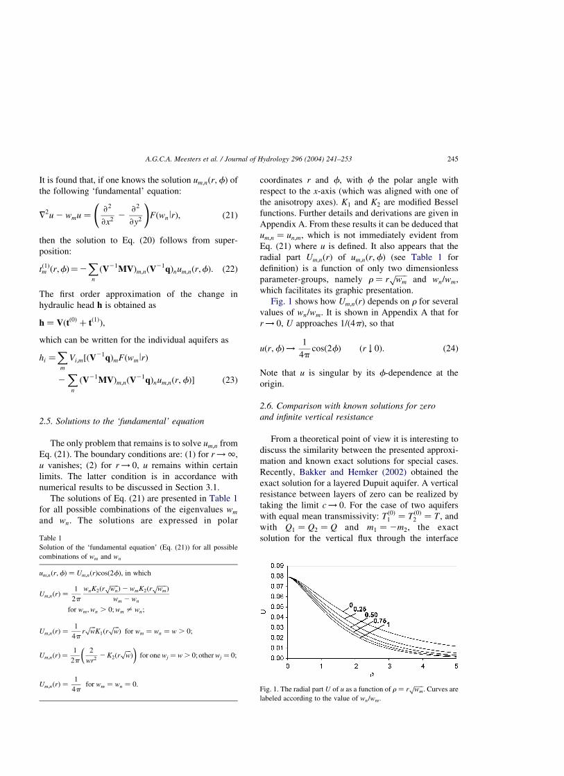
Fig. 1 shows how Um;nðrÞ depends on r for several

values of wn=wm: It is shown in Appendix A that for

r ! 0; U approaches 1=ð4pÞ; so that

uðr;fÞ!1

4pcosð2fÞ ðr # 0Þ: ð24Þ

Note that u is singular by its f-dependence at the

origin.

2.6. Comparison with known solutions for zero

and infinite vertical resistance

From a theoretical point of view it is interesting to

discuss the similarity between the presented approxi-

mation and known exact solutions for special cases.

Recently, Bakker and Hemker (2002) obtained the

exact solution for a layered Dupuit aquifer. A vertical

resistance between layers of zero can be realized by

taking the limit c ! 0: For the case of two aquifers

with equal mean transmissivity: T ð0Þ1 ¼ T ð0Þ

2 ¼ T ; and

with Q1 ¼ Q2 ¼ Q and m1 ¼ 2m2; the exact

solution for the vertical flux through the interfaceTable 1

Solution of the ‘fundamental equation’ (Eq. (21)) for all possible

combinations of wm and wn

um;nðr;fÞ ¼ Um;nðrÞcosð2fÞ; in which

Um;nðrÞ ¼1

2p

wnK2ðrffiffiffiffiwn

pÞ2 wmK2ðr

ffiffiffiffiwm

pÞ

wm 2 wn

for wm;wn . 0;wm – wn;

Um;nðrÞ ¼1

4prffiffiffiw

pK1ðr

ffiffiffiw

pÞ for wm ¼ wn ¼ w . 0;

Um;nðrÞ ¼1

2p

2

wr22K2ðr

ffiffiffiw

pÞ

� �for one wj ¼ w . 0;other wj ¼ 0;

Um;nðrÞ ¼1

4pfor wm ¼ wn ¼ 0:

Fig. 1. The radial part U of u as a function of r ¼ rffiffiffiffiwm

p: Curves are

labeled according to the value of wn=wm:


reduces to

limc#0

h2 2 h1

c¼

mQ

p

1

r2cosð2fÞ: ð25Þ

Eq. (23) yields the same result: It can be derived with

some effort that for c . 0

h2 2 h1

c¼

2mQ

cTu2;1ðr;fÞ

¼mQ

p

1

r22

1

cTK2ðr

ffiffiffiffiffiffi2=cT

pÞ

� �cosð2fÞ:

ð26Þ

In the limit as c ! 0; the argument of K2 becomes 1.

Since K2 is an exponentially decaying function of its

argument, the term with K2 becomes zero, complet-

ing the proof. In less symmetrical cases (T ð0Þ1 – T ð0Þ

2

and/or m1 – 2m2), the agreement holds only if

terms that are of second order in m are neglected (but

the proof is rather long-winded).

Let us now consider the case with infinite vertical

resistances, for which the aquifers become indepen-

dent. The exact solution for this case can be found

from the isotropic solution by a coordinate transform-

ation (Bruggeman, 1999), which yields for a leaky

aquifer

hðx; yÞ ¼21

2p

Q

T

1ffiffiffiffiffiffiffiffiffi1 2 m2

p K0

ffiffiw

pffiffiffiffiffiffiffiffiffiffiffiffiffiffiffiffiffiffiffiffiffiffi

x2

1 þ mþ

y2

1 2 m

s0@

1A ð27Þ

where w ¼ 1=ðcTÞ and T is the mean transmissivity

T ð0Þ1 : For a confined aquifer K0 must be replaced with

2 ln, andp

w with some r210 ; in which r0 is the radius

of influence. Application of the method of Sections

2.3–2.5 is easy, since the matrices are numbers in this

case. The solution is

hðr;fÞ ¼ 21

2p

Q

TK0ðrÞ þ

m

2rK1ðrÞcosð2fÞ

� �;

r ¼ rffiffiw

pð28Þ

for a leaky aquifer, and

hðr;fÞ ¼ 21

2p

Q

T2lnðrÞ þ

m

2cosð2fÞ

� �;

r ¼ r=r0 ð29Þ

for a confined aquifer. These solutions are equal to

the Taylor expansions of the exact solutions regarded

as functions of m; if terms of second and higher order

in m are neglected. The essential steps in the proof are

x2

1 þ mþ

y2

1 2 m¼

1 2 m cosð2fÞ

1 2 m2r2

¼ ð1 2 m cosð2fÞÞr2 þ Oðm2Þ;

ð30Þ

and K00 ¼ 2K1 (Eq. (A6)).

3. Examples

3.1. Comparison of analytical and numerical

results for two aquifer layers

The analytical approximation has been derived for

weak anisotropy. To validate the applicability of the

analytical approximation, anisotropic numerical

groundwater models are built with MicroFEM and

used to compare results. MicroFEM is a finite-element

model code for multiple-aquifer steady-state and

transient ground-water flow modeling. Confined,

phreatic, stratified and leaky multi-aquifer systems

can be simulated with a maximum of 20 aquifers and

50,000 nodes per layer (Diodato, 2000; Hemker et al.,

2004).

For all experiments described in this paper, the

finite-element grid (Fig. 2) has an octogonal shape,

with a radius of 2000 m (200 m for run E). The nodal

distances decrease from 200 m (20 m for run E) at the

model boundary to 1 m near the centre, where the well

is located. At the model boundaries, heads are kept

fixed. Only steady-state solutions are considered.

We first describe results for a leaky aquifer system

(Fig. 3) consisting of two layers (aquifers) separated

by a thin leaky layer (vertical resistance interface,

aquitard) and covered by an aquitard. Only the lower

aquifer 2 is assumed anisotropic. The x-axis is chosen

in the direction of maximum transmissivity. In all

cases, Q1 ¼ Q2 ¼ 75 m3 day21.

The specifications for the standard run are

indicated in Fig. 3. Fig. 4 shows the drawdowns for

the standard run, for both layers and along both

principal axes, according to MicroFEM simulations

(symbols) and the analytical approximation (lines).

It appears that the results obtained by both methods


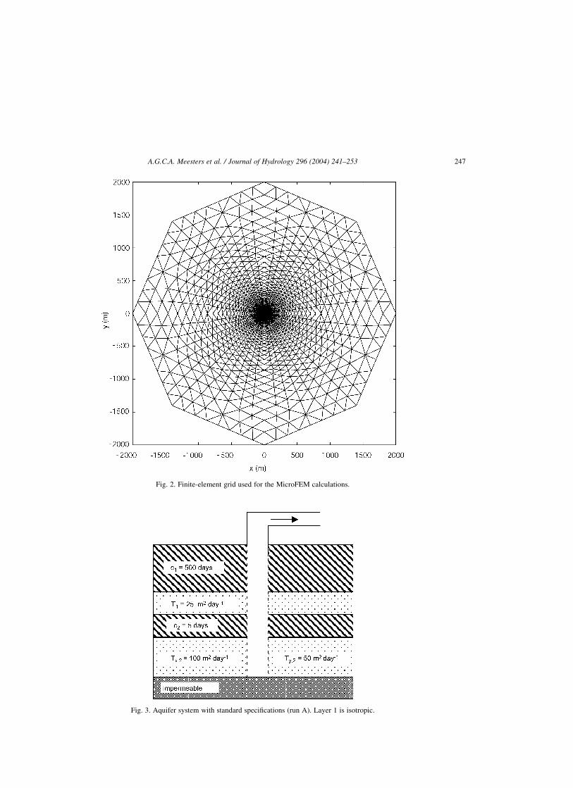
Fig. 2. Finite-element grid used for the MicroFEM calculations.

Fig. 3. Aquifer system with standard specifications (run A). Layer 1 is isotropic.


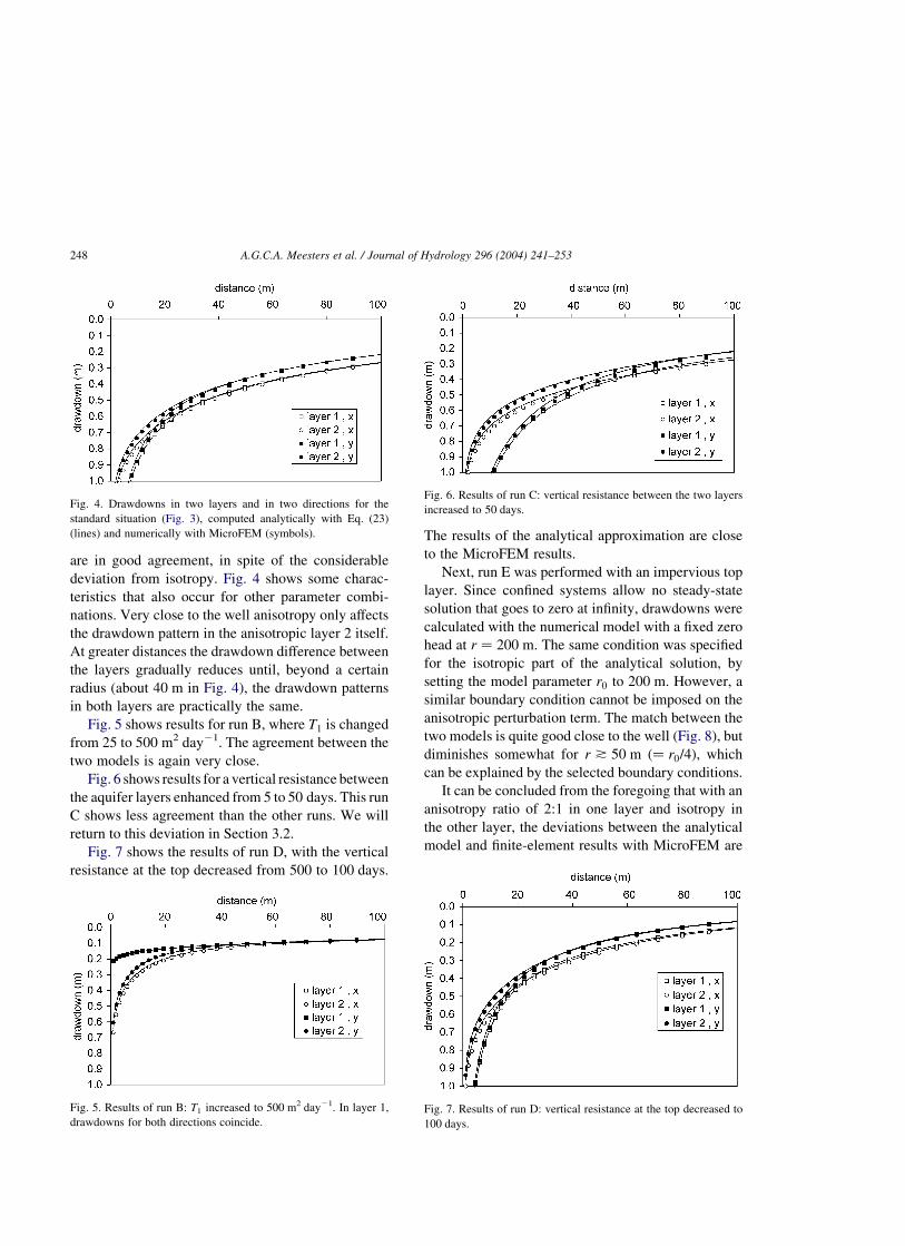
are in good agreement, in spite of the considerable

deviation from isotropy. Fig. 4 shows some charac-

teristics that also occur for other parameter combi-

nations. Very close to the well anisotropy only affects

the drawdown pattern in the anisotropic layer 2 itself.

At greater distances the drawdown difference between

the layers gradually reduces until, beyond a certain

radius (about 40 m in Fig. 4), the drawdown patterns

in both layers are practically the same.

Fig. 5 shows results for run B, where T1 is changed

from 25 to 500 m2 day21. The agreement between the

two models is again very close.

Fig. 6 shows results for a vertical resistance between

the aquifer layers enhanced from 5 to 50 days. This run

C shows less agreement than the other runs. We will

return to this deviation in Section 3.2.

Fig. 7 shows the results of run D, with the vertical

resistance at the top decreased from 500 to 100 days.

The results of the analytical approximation are close

to the MicroFEM results.

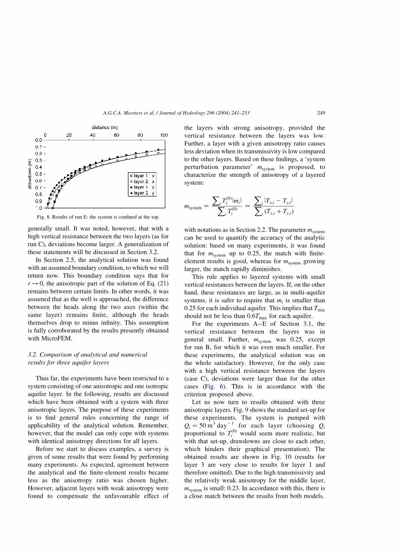
Next, run E was performed with an impervious top

layer. Since confined systems allow no steady-state

solution that goes to zero at infinity, drawdowns were

calculated with the numerical model with a fixed zero

head at r ¼ 200 m. The same condition was specified

for the isotropic part of the analytical solution, by

setting the model parameter r0 to 200 m. However, a

similar boundary condition cannot be imposed on the

anisotropic perturbation term. The match between the

two models is quite good close to the well (Fig. 8), but

diminishes somewhat for r * 50 m ð¼ r0=4Þ; which

can be explained by the selected boundary conditions.

It can be concluded from the foregoing that with an

anisotropy ratio of 2:1 in one layer and isotropy in

the other layer, the deviations between the analytical

model and finite-element results with MicroFEM are

Fig. 4. Drawdowns in two layers and in two directions for the

standard situation (Fig. 3), computed analytically with Eq. (23)

(lines) and numerically with MicroFEM (symbols).

Fig. 5. Results of run B: T1 increased to 500 m2 day21. In layer 1,

drawdowns for both directions coincide.

Fig. 6. Results of run C: vertical resistance between the two layers

increased to 50 days.

Fig. 7. Results of run D: vertical resistance at the top decreased to

100 days.


generally small. It was noted, however, that with a

high vertical resistance between the two layers (as for

run C), deviations become larger. A generalization of

these statements will be discussed in Section 3.2.

In Section 2.5, the analytical solution was found

with an assumed boundary condition, to which we will

return now. This boundary condition says that for

r ! 0; the anisotropic part of the solution of Eq. (21)

remains between certain limits. In other words, it was

assumed that as the well is approached, the difference

between the heads along the two axes (within the

same layer) remains finite, although the heads

themselves drop to minus infinity. This assumption

is fully corroborated by the results presently obtained

with MicroFEM.

3.2. Comparison of analytical and numerical

results for three aquifer layers

Thus far, the experiments have been restricted to a

system consisting of one anisotropic and one isotropic

aquifer layer. In the following, results are discussed

which have been obtained with a system with three

anisotropic layers. The purpose of these experiments

is to find general rules concerning the range of

applicability of the analytical solution. Remember,

however, that the model can only cope with systems

with identical anisotropy directions for all layers.

Before we start to discuss examples, a survey is

given of some results that were found by performing

many experiments. As expected, agreement between

the analytical and the finite-element results became

less as the anisotropy ratio was chosen higher.

However, adjacent layers with weak anisotropy were

found to compensate the unfavourable effect of

the layers with strong anisotropy, provided the

vertical resistance between the layers was low.

Further, a layer with a given anisotropy ratio causes

less deviation when its transmissivity is low compared

to the other layers. Based on these findings, a ‘system

perturbation parameter’ msystem is proposed, to

characterize the strength of anisotropy of a layered

system:

msystem ¼

XiT ð0Þ

i lmilXiT ð0Þ

i

¼

XilTx;i 2 Ty;ilX

iðTx;i þ Ty;iÞ

with notations as in Section 2.2. The parameter msystem

can be used to quantify the accuracy of the analytic

solution: based on many experiments, it was found

that for msystem up to 0.25, the match with finite-

element results is good, whereas for msystem growing

larger, the match rapidly diminishes.

This rule applies to layered systems with small

vertical resistances between the layers. If, on the other

hand, these resistances are large, as in multi-aquifer

systems, it is safer to require that mi is smaller than

0.25 for each individual aquifer. This implies that Tmin

should not be less than 0.6Tmax for each aquifer.

For the experiments A–E of Section 3.1, the

vertical resistance between the layers was in

general small. Further, msystem was 0.25, except

for run B, for which it was even much smaller. For

these experiments, the analytical solution was on

the whole satisfactory. However, for the only case

with a high vertical resistance between the layers

(case C), deviations were larger than for the other

cases (Fig. 6). This is in accordance with the

criterion proposed above.

Let us now turn to results obtained with three

anisotropic layers. Fig. 9 shows the standard set-up for

these experiments. The system is pumped with

Qi ¼ 50 m3 day21 for each layer (choosing Qi

proportional to T ð0Þi would seem more realistic, but

with that set-up, drawdowns are close to each other,

which hinders their graphical presentation). The

obtained results are shown in Fig. 10 (results for

layer 3 are very close to results for layer 1 and

therefore omitted). Due to the high transmissivity and

the relatively weak anisotropy for the middle layer,

msystem is small: 0.23. In accordance with this, there is

a close match between the results from both models.

Fig. 8. Results of run E: the system is confined at the top.


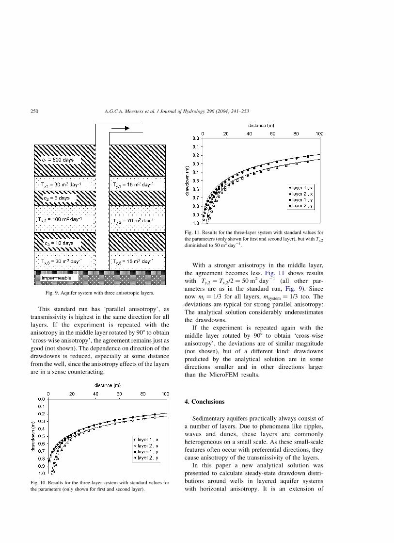
This standard run has ‘parallel anisotropy’, as

transmissivity is highest in the same direction for all

layers. If the experiment is repeated with the

anisotropy in the middle layer rotated by 908 to obtain

‘cross-wise anisotropy’, the agreement remains just as

good (not shown). The dependence on direction of the

drawdowns is reduced, especially at some distance

from the well, since the anisotropy effects of the layers

are in a sense counteracting.

With a stronger anisotropy in the middle layer,

the agreement becomes less. Fig. 11 shows results

with Ty;2 ¼ Tx;2=2 ¼ 50 m2 day21 (all other par-

ameters are as in the standard run, Fig. 9). Since

now mi ¼ 1=3 for all layers, msystem ¼ 1=3 too. The

deviations are typical for strong parallel anisotropy:

The analytical solution considerably underestimates

the drawdowns.

If the experiment is repeated again with the

middle layer rotated by 908 to obtain ‘cross-wise

anisotropy’, the deviations are of similar magnitude

(not shown), but of a different kind: drawdowns

predicted by the analytical solution are in some

directions smaller and in other directions larger

than the MicroFEM results.

4. Conclusions

Sedimentary aquifers practically always consist of

a number of layers. Due to phenomena like ripples,

waves and dunes, these layers are commonly

heterogeneous on a small scale. As these small-scale

features often occur with preferential directions, they

cause anisotropy of the transmissivity of the layers.

In this paper a new analytical solution was

presented to calculate steady-state drawdown distri-

butions around wells in layered aquifer systems

with horizontal anisotropy. It is an extension of

Fig. 9. Aquifer system with three anisotropic layers.

Fig. 10. Results for the three-layer system with standard values for

the parameters (only shown for first and second layer).

Fig. 11. Results for the three-layer system with standard values for

the parameters (only shown for first and second layer), but with Ty;2

diminished to 50 m2 day21.


the eigenvalue method proposed by Hemker (1984),

the new feature being the inclusion of anisotropy. It is

assumed that only one aquifer layer is anisotropic or,

when more layers are anisotropic, that the directions

of anisotropy are the same for all layers. Moreover,

the results are only valid as an approximation for

weak anisotropy.

It was demonstrated that the approximation

behaves asymptotically correct when the vertical

resistances of the aquitards become zero or infinitely

large.

The analytical solution has been tested by

comparing results to those of the finite-element

model MicroFEM, for many two and three-layer

cases. The accuracy of the results depends on the

anisotropy ratios of all aquifer layers. Limiting

conditions are proposed for the applicability of the

analytic approximation, for both layered aquifers and

multi-aquifer systems.

The analytical solution has a limited application

scope as it is restricted to horizontally homogeneous

systems, steady-state flow, and limited anisotropy.

The model is useful for theoretical research. More-

over, since computations appear to be fast, the model

is attractive for repetitive drawdown calculations as

typically required for automatic parameter estimation

when analyzing pumping test data. Experiments with

synthetic data (which we do not discuss in this paper)

have demonstrated the feasibility of such

calculations.

Acknowledgements

The authors thank C. Fitts and F. Szekely for their

comments and suggestions.

Appendix A

A.1. Formulation of the problem

This appendix is devoted to solving the equation

72u 2 w1u ¼›2

›x22

›2

›y2

!Fðw2lrÞ ðA1Þ

in which uðr;fÞ is the unknown function, w1 and w2

are known constants (positive or zero), and F is

defined as

w2 . 0 : Fðw2lrÞ ¼ 21

2pK0ðr

ffiffiffiffiw2

pÞ; ðA2aÞ

w2 ¼ 0 : Fðw2lrÞ ¼1

2plnðr=r0Þ: ðA2bÞ

Note that F is singular for r ¼ 0: It will be shown

below that the solution for w2 . 0 turns in to the

solution for w2 ¼ 0 in the limit w2 ! 0: As boundary

conditions we assume that u vanishes for r !1; and

that u remains finite for r ! 0: It follows from general

principles that the problem has a unique solution.

A.2. Auxiliary properties of modified Bessel functions

Two properties will be used repeatedly in this

exposition. The first is the Helmholtz-equation

f ðr;fÞ ¼ Knðrffiffiw

pÞcosðnfÞ or

f ðr;fÞ ¼ Knðrffiffiw

pÞsinðnfÞ ) 72f ¼ wf

ðA3Þ

for r . 0 and n ¼ 0;1,2,… (e.g. Arfken, 3rd edition,

1985; not in older editions). The second is the

approximation for small radial arguments:

K2ðrÞ <2

r22

1

2þ Oðr2 ln rÞ ðr # 0Þ ðA4Þ

(adapted from Abramowitz and Stegun, 1965,

Eq. (9.6.11)).

Other equations, which will be incidentally

invoked, are the modified Bessel equation for n ¼ 0 :

K 000ðrÞ þ

1

rK 0

0ðrÞ2 K0ðrÞ ¼ 0 ðA5Þ

(Abramowitz and Stegun, Eq. (9.6.1)); and the

recurrence relations

K 00 ¼ 2K1 ðA6Þ

K 02 ¼ 2

2

rK2 2 K1 ðA7Þ

2

rK1 ¼ K2 2 K0 ðA8Þ

(Abramowitz and Stegun 9.6.26).


A.3. Evaluation of the right hand side

We now consider the evaluation of the right hand

side of Eq. (A1). It is found that for positive w

2›2

›x22

›2

›y2

!K0ðr

ffiffiw

pÞ ¼ 2wK2ðr

ffiffiw

pÞcosð2fÞ

ðA9Þ

Sketch of the proof: Expressing the left hand side in

polar coordinates, one finds:

2w K 000ðr

ffiffiw

pÞ2

1

rffiffiw

p K 00ðr

ffiffiw

pÞ

� cosð2fÞ;

subsequent application of (A5), (A6), and (A8), yields

(A9).

For the case that w ¼ 0; (A2b), it is found by

applying common calculus rules that

›2

›x22

›2

›y2

!lnðr=r0Þ ¼ 2

2

r2cosð2fÞ: ðA10Þ

This outcome is the limit for w2 ! 0 of the right hand

side of (A9), as is seen by using (A4). As a

consequence, the solution of (A1) for w2 ¼ 0 can be

found by taking the solution for positive w2; and

letting w2 go to 0.

A.4. Solutions for positive w1 and w2

Now we can commence solving (A1), starting with

the case w1; w2 . 0; so that

72u 2 w1u ¼ 21

2pw2K2ðr

ffiffiffiffiw2

pÞcosð2fÞ: ðA11Þ

We first consider the homogenous counterpart, which

is the Helmholtz-equation. Independent solutions are

given by (A3). Other independent solutions, with In

instead Kn; do exist, but they are unsuited since they

grow exponentially as r !1: Hence the complete

solution of the homogenous equation is

X1n¼0

Knðrffiffiffiffiw1

pÞ½cn cosðnfÞ þ dn sinðnfÞ�: ðA12Þ

On the other hand, we can link the left and right hand

side of (A11) by noting that it follows from (A3) that

ð72 2 w1ÞðK2ðrffiffiffiffiw2

pÞcosð2fÞÞ

¼ ðw2 2 w1ÞK2ðrffiffiffiffiw2

pÞcosð2fÞ; ðA13Þ

hence, a particular solution of (A11) is

1

2p

w2

w1 2 w2

K2ðrffiffiffiffiw2

pÞcosð2fÞ; ðA14Þ

provided w1 – w2 (the case w1 ¼ w2 will be con-

sidered below).

The complete solution of (A11) is the sum of

(A12) and (A14). However, this solution does not

yet match the boundary condition that u remains

finite for r ! 0: Actually, all terms in the solution

violate this condition (Kn becomes infinite as r

goes to 0). Hence their singularities should cancel

each other; noting the fact that all terms have

different angular dependence, expect the two with

cosð2fÞ; it follows that c2 must be chosen so that

these latter two terms cancel, whereas all other cn

and all dn must be zero. The proper choice for c2

is 2w1=ð2pðw1 2 w2ÞÞ; as follows by working out

the singularities with (A4). So we finally obtain a

solution for our problem:

uðr;fÞ ¼1

2p

w2K2ðrffiffiw

p2Þ2 w1K2ðr

ffiffiw

p1Þ

w1 2 w2

cosð2fÞ

ðw1;w2 . 0;w1 – w2Þ: ðA15Þ

It follows from (A4) that for small r

uðr;fÞ ¼1

4pþ Oðr2 ln rÞ ðr # 0Þ

ðwith r ¼ rffiffiw

pÞ: ðA16Þ

For the special case that w1 ¼ w2; the solution is

uðr;fÞ ¼1

4prffiffiffiffiw1

pK1ðr

ffiffiffiffiw1

pÞcosð2fÞ

ðw1 ¼ w2 . 0Þ: ðA17Þ

This follows from (A15) by taking the limit w2 !

w1: Proof: Both numerator and denominator


becomes zero; Applying L’Hopital’s rule yields:

limw2!w1

uðr;fÞ ¼21

2pK2ðr

ffiffiffiffiw1

pÞþ

1

2rffiffiffiffiw1

pK 0

2ðrffiffiffiffiw1

pÞ

�

� cosð2fÞ;

and to this (A7) is applied.

A.5. The case that w1 ¼ 0 and/or w2 ¼ 0

Eq. (A1) with (A2b) can now be solved easily by

taking the limit w2 ! 0 (as allowed for in Section

A.3). This yields, using Eq. (A4)

uðr;fÞ ¼1

2p

2

w1r22 K2ðr

ffiffiffiffiw1

pÞ

� cosð2fÞ

ðw1 . 0;w2 ¼ 0Þ: ðA18Þ

We now turn to the case w1 ¼ 0: The solution to

(A1) is found by taking the limit w1 ! 0 in (A15),

yielding of course the same as (A18) but with w2 in

the role of w1 :

uðr;fÞ ¼1

2p

2

w2r22 K2ðr

ffiffiffiffiw2

pÞ

� cosð2fÞ

ðw1 ¼ 0;w2 . 0Þ: ðA19Þ

Finally, the limit with both w1 ! 0 and w2 ! 0 is

easily found from (A18) or (A19), using (A4), to be

uðr;fÞ ¼1

4pcosð2fÞ

ðw1 ¼ 0;w2 ¼ 0Þ: ðA20Þ

All these limit-solutions can be verified by substi-

tution. One should then use, besides (A3):

72 1

r2cosð2fÞ

� �¼ 0;

72ðcosð2fÞÞ ¼ 24

r2cosð2fÞ:

References

Abramowitz, M., Stegun, I.A., 1965. Handbook of Mathematical

Functions, Dover, New York.

Arfken G., 1985. Mathematical Methods for Physicists (3rd ed.),

Orlando, etc.

Bakker, M., Hemker, K., 2002. : A Dupuit formulation for flow in

layered, anisotropic aquifers. Advances in Water Resources

25(7), 747–754.

Bruggeman, G.A., 1999. Analytical solutions of geohydrological

problems, Developments in Water Science, Vol. 46. Elsevier,

Amsterdam.

Diodato, D.M., 2000. Software Spotlight MicroFem Version 3.50.

Ground Water 38(5), 649–650.

Freeze, R.A., Cherry, J.A., 1979. Groundwater, Prentice-Hall,

Englewood Cliffs, NJ.

Getzen, R.T., 1983. Soil mechanics related to permeability

anisotropy of coastal sand deposits. In: Magoon, O.T.,

Converse, H. (Eds.), Coastal zone ’83: Proceedings of the

Symposium on Coastal and Ocean Management, American

Society of Civil Engineers, New York, pp. 2413–2430.

Hemker, C.J., 1984. Steady groundwater flow in leaky multiple-

aquifer systems. Journal of Hydrology 72, 355–374.

Hemker, K., van den Berg, E., Bakker, M., 2004. Ground water

whirls. Ground Water 42, 234–242.

Lebbe, L., De Breuck, W., 1997. Analysis of a pumping test in an

anisotropic aquifer by use of an inverse numerical model.

Hydrogeology Journal 5(3), 44–59.

Maas, C., 1987. Groundwater flow to a well in a layered porous

medium 1. Steady flow. Water Resources Research 23(8),

1675–1681.

McDonald, M.G., Harbaugh, A.W., 1988. A modular three-

dimensional finite-difference ground-water flow model.

U.S.G.S. Techniques of Water-Resources Investigations, Book

6, chapter Al.

Nakaya, S., Yohmei, T., Koike, A., Hirayama, T., Yoden, T.,

Nishigaki, M., 2002. Determination of anisotropy of spatial

correlation structure in a three-dimensional permeability field

accompanied by shallow faults. Water Resources Research

38(8) art. no. 1160.

Pickup, G.E., Ringrose, P.S., Jensen, J.L., Sorbie, K.S., 1994.

Permeability tensor for sedimentary structures. Mathematical

Geology 26(2), 227–250.

Van den Berg, E.H., 2003. The impact of primary sedimentary

structures on groundwater flow—a multi-scale sedimentological

and hydrogeological study in unconsolidated eolian dune

deposits. PhD Thesis, Vrije Universiteit Amsterdam, 196 pp.


Documents

An approximate analytical solution for well flow in anisotropic layered aquifer systems