Receiver Functions of Seismic Waves in Layered Anisotropic ...rses.anu.edu.au/~nick/teachdoc/papers/Nagaya_etal_RF_BSSA08.pdf · Receiver Functions of Seismic Waves in Layered Anisotropic

Receiver Functions of Seismic Waves in Layered Anisotropic Media:

Application to the Estimate of Seismic Anisotropy

by Mamoru Nagaya, Hitoshi Oda, Hirokazu Akazawa, and Motoko Ishise

Abstract We investigate the effect of seismic anisotropy on P-wave receiver func-tions, calculating synthetic seismograms for P-wave incidence on multilayered aniso-tropic structure with hexagonal symmetry. The main characteristics of the receiverfunctions affected by the anisotropy are summarized as (1) appearance of seismicenergy on radial and transverse receiver functions, (2) systematic change of P-to-S(Ps) converted waveforms on receiver functions as ray back-azimuth increases, and(3) reversal of the Ps-phase polarity on the radial receiver function in a range of theback azimuth. Another important influence is shear-wave splitting of the Ps-convertedwaves and other later phases reverberated as S wave. By numerical experiments usingsynthetic receiver functions, we demonstrate that the waveform cross-correlationanalysis is applicable to splitting Ps phases on receiver functions to estimate the seis-mic anisotropy of layer structure. Advantages to utilizing the Ps phases are (1) theyappear more clearly on receiver functions than on seismograms and (2) they inform usabout what place along the seismic ray path is anisotropic. Real analysis of shear-wavesplitting is executed to the Moho-generated Ps phases that are identified on receiverfunctions at six seismic stations in the Chugoku district, southwest Japan. The timelags between the two arrivals of the split Ps phases are estimated at 0.2–0.7 sec, andthe polarization directions of the fast arrival components are from north–south tonortheast–southwest. This result is consistent with recent results of shear-wave split-ting measurements and the trend of linear epicenter distributions of crustal earth-quakes and active fault strikes in the Chugoku district.

Introduction

The observations of shear-wave splitting have beenwidely performed to detect seismic anisotropy in the crustand mantle (e.g., Ando, 1984; Fukao, 1984; Silver andChang; 1988; Kaneshima, 1990). The shear-wave splittingis effective to diagnose that seismic anisotropy resides some-where on a propagation path of shear wave, but it has theinherent shortcoming that the depth resolution is poor to findwhat zone on the ray path is anisotropic. If antecedents ofseismic waves that we are going to analyze are exactlyknown, such as the Ps phase generated by P-to-S conversionat a velocity discontinuity, the shortcoming would be circum-vented. Thus, we intend to utilize the Ps-converted waves toestimate the anisotropic velocity structure in the crust andupper mantle. The Ps phase travels as a shear wave afterthe P-to-S conversion at the velocity discontinuity, so it isthought to have the characteristic of shear-wave splitting be-cause of shear-wave polarization anisotropy that is caused byseismic anisotropy in layers above the discontinuity, that is,the Ps wave splits into two components that propagate withdifferent velocities. If the polarization anisotropy of the Psphase is detected by shear-wave splitting analysis, it provides

us with information about the seismic anisotropy in layersoverlying the discontinuity; consequently, we know whatplace along the seismic ray path is anisotropic. However,clear Ps-converted waves to which the shear-wave splittinganalysis is applicable are rarely recorded on observed seis-mograms from local earthquakes because of complexities ofsource time functions and contaminations of noise and otherseismic phases.

We think that the P-wave receiver function can beutilized to identify clear Ps-converted waves, because thesource time function is eliminated from it. The receiverfunction method has been developed to find velocity discon-tinuities beneath various regions and to estimate their three-dimensional configurations (e.g., Langston, 1979; Owenset al., 1984; Shibutani et al., 1996; Peng and Humphreys,1998; Zhu and Kanamori, 2000; Yamauchi et al., 2003).The method is excellent at clearly showing the Ps phaseson the receiver functions even if seismograms are contami-nated by noise and scattering waves. Thus, we intend toexecute shear-wave splitting analysis to the Ps phases on re-ceiver functions. The first attempt to measure the shear-wave

2990

Bulletin of the Seismological Society of America, Vol. 98, No. 6, pp. 2990–3006, December 2008, doi: 10.1785/0120080130

splitting of the Ps phase was made by McNamara and Owens(1993). Further, how the seismic anisotropy influences thePs phases on receiver functions was theoretically and obser-vationally examined by subsequent studies (e.g., Levin andPark, 1997, 1998; Peng and Humphreys, 1997; Savage,1998). These studies showed that the polarization anisotropywas detectable by the splitting analysis of the Ps phases onthe receiver functions. In this study, we review the effect ofseismic anisotropy on the Ps phases, calculating syntheticreceiver functions for layered structures of isotropic and an-isotropic velocities, and we address some issues on the split-ting analysis of the Ps phases.

The splitting analysis is really carried out to Ps-converted waves on P-wave receiver functions obtained fromteleseismic waveform data at seismic stations in the Chugokudistrict, southwest Japan. What we measure by the analysis isthe fast polarization direction of two components of splittingPs phase and the time lag between two arrivals of the split Psphase. It is well known in the crust that the fast polarizationdirections of direct S waves are nearly parallel to trajectoriesof maximum principal stress acting on the Japan Islands(Kaneshima, 1990). The crustal anisotropy is interpretedas being due to crack-induced anisotropy, which is causedby the alignment of open cracks produced by the maximumprincipal stress (Crampin, 1981). In the Chugoku district, thedirection of maximum principal stress is known to be in anearly northwest–southeast direction (Ando, 1979; Tsuka-hara and Kobayashi, 1991). Thus, the fast polarization direc-tion of the shear wave is expected to be in the same directionas the maximum principal stress. But Iidaka (2003) reportedby the splitting analysis of two phases reverberated in thecrust that the fast polarization directions were inconsistentwith the maximum principal stress direction in southwest Ja-pan. This result may arise because the seismic phases ana-lyzed in Iidaka’s study were not clear enough to apply thesplitting analysis. Recently, high-quality seismic waveformdata from the F-net, which is a broadband seismic networkdeployed over Japan, were analyzed for study of seismic an-isotropy in the upper mantle under the Japan Islands (e.g.,Long and van der Hilst, 2005, 2006). In this article, after cal-culating P-wave receiver functions from the seismic recordsat the F-net stations and temporal stations in the Chugokudistrict, we find clear Ps phases converted at the Moho dis-continuity. The fast polarization direction and the delay timesare estimated by the splitting analysis of the Ps phases on thereceiver functions. In addition, we investigate regional var-iation of the seismic anisotropy within the crust and examinethe relationship between lateral variation of the fast polariza-tion direction and tectonic stress acting on southwest Japan.

Description of Anisotropic Structure and CalculationMethod of Receiver Functions

The study of seismic-wave propagation in layered aniso-tropic structure was started by Crampin (1970); subsequentstudies were done for complicated velocity structures includ-

ing seismic anisotropy and dipping velocity discontinuity(e.g., Keith and Crampin, 1977a,b; Levin and Park, 1977;Fryer and Frazer, 1984; Savage, 1998, Frederiksen and Bo-stock, 2000). In this section, we explain the parameters usedto describe anisotropic velocity structure and briefly presenthow to calculate synthetic seismograms and receiver func-tions of seismic body waves propagating into a stratified an-isotropic medium.

Olivine and enstatite crystals, the major anisotropicminerals in peridotite (which is considered to be a candidateof upper mantle material), possess orthorhombic symmetry(Anderson, 1989), but the elastic behavior of typical perido-tite samples is well approximated by hexagonal symmetry(Montagner and Anderson, 1989; Mainprice and Silver,1993). Hexagonal symmetry is also appropriate for the elas-tic property of the medium containing aligned cracks, such asthe upper crust (Crampin, 1978; Hudson, 1981; Kaneshima,1991). Therefore, the upper mantle and the crust are assumedto have seismic anisotropy of hexagonal symmetry. The seis-mic velocity perturbations arising from weak hexagonal an-isotropy are written as (Backus 1965; Park and Yu 1992)

!!2 " !20#=!2

0 $ A% B cos 2"% C cos 4"; for P wave

!#2 " #20#=#2

0 $ D% E cos 2"; for S wave; (1)

where ! and # are the P- and S-wave velocities, respectively,and " is the angle between the hexagonal-symmetry axis andthe propagation direction of the seismic wave. Parameterswith subscript 0 denote the isotropic velocities of P and Swaves. Dimensionless parameters (B, C, and E) denote theanisotropic velocity perturbations, and A and D are the iso-tropic velocity perturbations. When the c axis in Cartesiancoordinates of !a; b; c#! !1; 2; 3# is taken as the hexagonal-symmetry axis, the elastic constants Cijkl are written as fol-lows (Park and Yu, 1992):

C1111 $ C2222 $ !1% A " B% C#$!20;

C3333 $ !1% A% B% C#$!20;

C1122 $ !1% A " B% C#$!20 " 2!1%D " E#$#2

0;

C1133 $ C2233 $ !1% A " 3C#$!20 " 2!1%D% E#$#2

0;

C1313 $ C2323 $ !1% A% B% C#$#20;

C1212 $ !C1111 " C1122#=2; (2)

where $ is the density. Further, the elastic constants satisfythe relationship of

Cijkl $ Cjikl $ Cijlk $ Cklij: (3)

The elastic constants other than those specified by equa-tions (2) and (3) are equal to zero. Another Cartesiancoordinate system of !x1; x2; x3#! !10; 20; 30# is set in asemi-infinite layered medium, where the ground surface isthex1 " x2 plane and the x3 axis is taken vertically downward

Receiver Functions of Seismic Waves in Layered Anisotropic Media 2991

to the ground surface. The elastic constants Cijkl are trans-formed into those ci0j0k0l0 defined in the !x1; x2; x3# coordinatesystem through

ci0j0k0l0 $ Uii0Ujj0Ukk0Ull0Cijkl: (4)

The matrix elements Uii0 are given by

U $cos % cos & cos % sin & " sin %" sin& cos & 0

sin % cos & sin % sin& cos %

0

@

1

A; (5)

where % is the tilt angle of the hexagonal-symmetry axis mea-sured from the x3 axis; & is the azimuth of the symmetry axismeasured clockwise from the north (x1 axis). Thus, the elas-tic constants ci0j0k0l0 are calculated by using equation (4) if wespecify the dimensionless parameters !A; B; C;D; E# of iso-tropic and anisotropic velocity perturbations, the orientationof hexagonal-symmetry axis !%;&#, the isotropic velocities ofP and S waves !!0; #0#, and the density$.

Synthetic seismograms of seismic waves travelingthrough a horizontally layered structure are calculated byusing the equation

ui!t# $ hi!t# & s!t#; (6)

where ui!t# and hi!t# are the ith components of the dis-placement vector and transfer functions, respectively, s!t#denotes the earthquake source time function, and the sym-bol & represents the convolution operator. The layer matrixmethod of Crampin (1970) is employed to calculate thetransfer functions hi!t# of the layered anisotropic structure,each layer of which is specified by eleven parameters!!0; #0; $; A; B; C;D; E; %;&# and layer thickness d. Radialand transverse receiver functions are defined for two pairsof radial and vertical component seismograms and of trans-verse and vertical component seismograms, respectively. Ac-cording to Langston (1979), Fourier transform of the receiverfunction ri!t# is written as

Ri!'# $Ui!'# !UZ!'#

(!'#e"'

2=4a2 ; (7)

where ' is the angular frequency, Ui!'# denotes Fouriertransform of ui!t#, !Uz!'# represents the complex conjugateofUz!'#, a is the parameter to control the width of the Gaus-sian filter, and

(!'# $ maxfUz!'# !Uz!'#; cmax'Uz!'# !Uz!'#(g: (8)

Here c denotes the water level. The receiver functions ri!t# inthe time domain are obtained by calculating the inverse Fou-rier transform of Ri!'#, and their radial and transverse com-ponents are specified by replacing the subscript i with R andT, respectively.

The Effect of Seismic Anisotropyon Receiver Functions

We calculate synthetic seismograms and receiver func-tions for several models of layered anisotropic structure,assuming that a plane P wave is incoming from the isotro-pic bottom layer to the anisotropic structure. The incidentangle is set at 10° measured from the vertical. One cyclesinusoidal wave with a period of 2 sec is assumed forthe incident P wave. The values of the layer parameters!!0; #0; $; d; A; B; C;D; E; %;&# of the velocity models arelisted in Tables 1, 2, and 3. We set C $ 0 in the models be-cause the cos 4" term in equation (1) may be negligibly smallin the upper mantle and crust (e.g., Park and Yu, 1992; Ishiseand Oda, 2005, 2008). Figure 1a depicts synthetic seismo-grams calculated for a two-layered anisotropic structure(Model 1a) that consists of a 35 km thick anisotropic surfacelayer and isotropic bottom layer (Table 1). In the anisotropicsurface layer, the symmetry axis lies horizontally in a north–south direction. Ray back azimuth of the incident wave is setat 45°, measured clockwise from the north. Because of theelasticity of hexagonal symmetry, both the radial and trans-verse components are excited. For comparison, synthetic

Table 1Parameter Values of Model 1

Model 1a Model 1b

Layer Number !0 !km=sec# #0 !km=sec# $ !g=cm3# d (km) B E & (°) % (°) & (°) % (°)

1 6.7 3.8 2.7 35.0 0.02 0.04 0.0 90.0 0.0 45.02 7.8 4.5 3.3 0.0 0.00 0.00 — — — —


Model 2a Model 2b

Layer Number !0 !km=sec# #0 !km=sec# $ !g=cm3# d (km) B E &(°) % (°) &(°) % (°)

1 5.8 3.6 2.8 35.0 — — — — — —2 7.2 4.0 3.2 35.0 0.02 0.04 0.0 90.0 0.0 45.03 8.0 4.3 3.6 0.0 0.00 — — — — —

2992 M. Nagaya, H. Oda, H. Akazawa, and M. Ishise

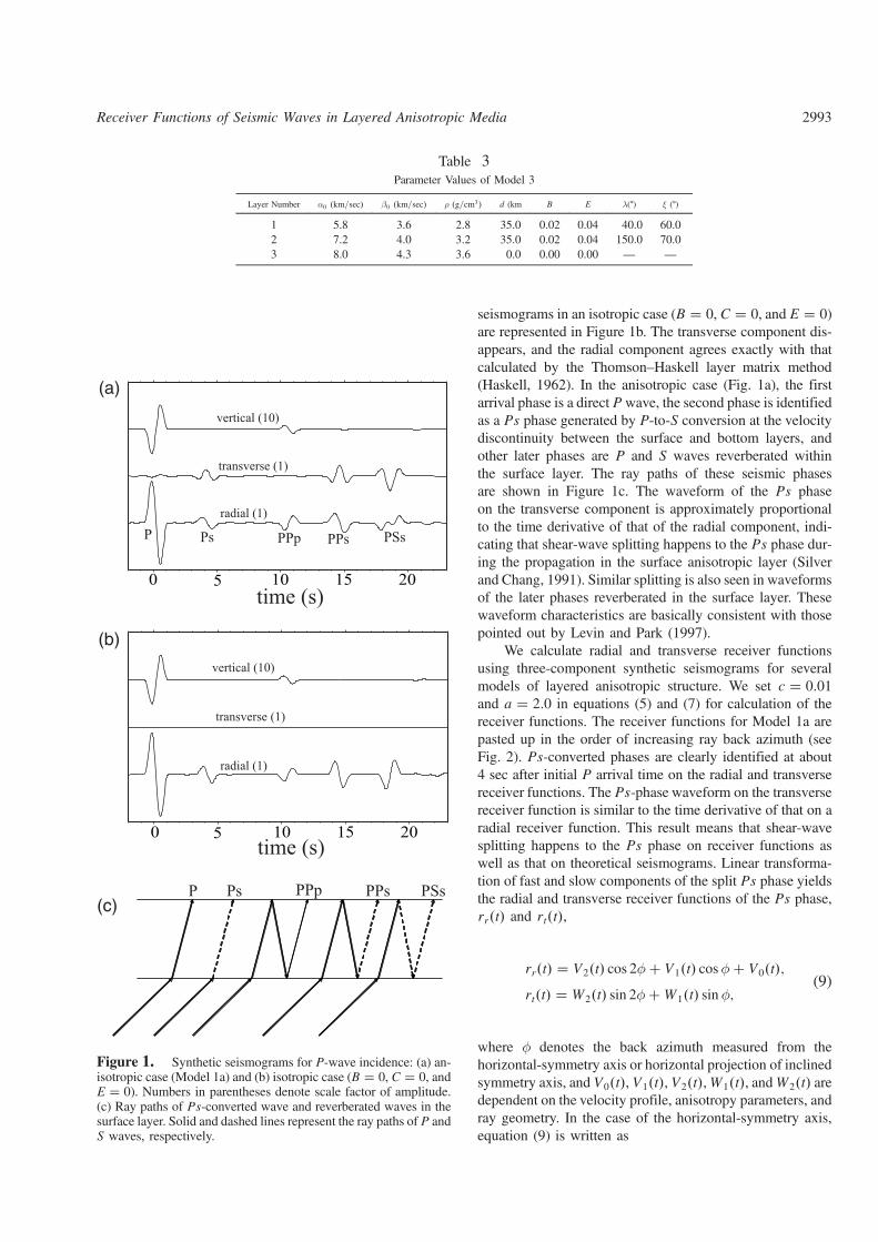
seismograms in an isotropic case (B $ 0, C $ 0, and E $ 0)are represented in Figure 1b. The transverse component dis-appears, and the radial component agrees exactly with thatcalculated by the Thomson–Haskell layer matrix method(Haskell, 1962). In the anisotropic case (Fig. 1a), the firstarrival phase is a direct Pwave, the second phase is identifiedas a Ps phase generated by P-to-S conversion at the velocitydiscontinuity between the surface and bottom layers, andother later phases are P and S waves reverberated withinthe surface layer. The ray paths of these seismic phasesare shown in Figure 1c. The waveform of the Ps phaseon the transverse component is approximately proportionalto the time derivative of that of the radial component, indi-cating that shear-wave splitting happens to the Ps phase dur-ing the propagation in the surface anisotropic layer (Silverand Chang, 1991). Similar splitting is also seen in waveformsof the later phases reverberated in the surface layer. Thesewaveform characteristics are basically consistent with thosepointed out by Levin and Park (1997).

We calculate radial and transverse receiver functionsusing three-component synthetic seismograms for severalmodels of layered anisotropic structure. We set c $ 0:01and a $ 2:0 in equations (5) and (7) for calculation of thereceiver functions. The receiver functions for Model 1a arepasted up in the order of increasing ray back azimuth (seeFig. 2). Ps-converted phases are clearly identified at about4 sec after initial P arrival time on the radial and transversereceiver functions. The Ps-phase waveform on the transversereceiver function is similar to the time derivative of that on aradial receiver function. This result means that shear-wavesplitting happens to the Ps phase on receiver functions aswell as that on theoretical seismograms. Linear transforma-tion of fast and slow components of the split Ps phase yieldsthe radial and transverse receiver functions of the Ps phase,rr!t# and rt!t#,

rr!t# $ V2!t# cos 2)% V1!t# cos)% V0!t#;

rt!t# $ W2!t# sin 2)%W1!t# sin);(9)

where ) denotes the back azimuth measured from thehorizontal-symmetry axis or horizontal projection of inclinedsymmetry axis, and V0!t#, V1!t#, V2!t#,W1!t#, andW2!t# aredependent on the velocity profile, anisotropy parameters, andray geometry. In the case of the horizontal-symmetry axis,equation (9) is written as


Layer Number !0 !km=sec# #0 !km=sec# $ !g=cm3# d (km B E &(°) % (°)

1 5.8 3.6 2.8 35.0 0.02 0.04 40.0 60.02 7.2 4.0 3.2 35.0 0.02 0.04 150.0 70.03 8.0 4.3 3.6 0.0 0.00 0.00 — —

P Ps PPp PPs PSs

(b)

vertical (10)

transverse (1)

radial (1)

0 5 10 2015time (s)

(c)

P Ps PPp PPs PSs

(a)

0 5 10 15 20time (s)

vertical (10)

radial (1)

transverse (1)

Figure 1. Synthetic seismograms for P-wave incidence: (a) an-isotropic case (Model 1a) and (b) isotropic case (B $ 0, C $ 0, andE $ 0). Numbers in parentheses denote scale factor of amplitude.(c) Ray paths of Ps-converted wave and reverberated waves in thesurface layer. Solid and dashed lines represent the ray paths of P andS waves, respectively.


rr!t# $ a!t% *t=2#!cos)#2 % a!t " *t=2#!sin)#2;

rt!t# $ "fa!t% *t=2# " a!t " *t=2#g sin) cos);(10)

where a!t% *t=2# and a!t " *t=2# denote the receiver func-tion waveforms of fast and slow components of the split Psphase, respectively, and *t is the time lag between their ar-rivals. The transverse receiver functions in Figure 2 show thatthe initial motions of direct P wave and Ps-converted wavehave the same polarity and that their amplitude variationsversus ) exhibit a four-lobed pattern (sin 2)), which can beeasily understood by using equation (10). Thus, the directP wave and Ps phase disappear when the incident directionis parallel or normal to the hexagonal-symmetry axis in thenorth. The four-lobed pattern of amplitude variation is alsoseen in the reverberated later phases. On the other hand, thePs phase on the radial receiver function shows the azimuthalamplitude variation that would be expressed by a!t# "*a!t# cos 2), which is an approximate expression of equa-tion (10). In addition, peak arrival time of the Ps phaseversus ) exhibits four-lobed modulation that would be writ-ten as t0 " *t cos 2), where t0 denotes the reference arrivaltime. The arrival-time modulation can be understood when

the amplitude variation of a!t# " *a!t# cos 2) is taken intoaccount. But the arrival-time modulation is not seen in thePs phase on the transverse component because the transversePs waveform in equation (10) is approximately expressedby *a!t# sin 2).

Figure 3 shows radial and transverse receiver functionsfor Model 1b, in which the hexagonal-symmetry axis is in-clined toward the north (see Table 1). On the transverse re-ceiver functions, the amplitude variations of direct P waveand Ps phase show a two-lobed pattern depending on sin),where ) is measured from the horizontal projection of theinclined symmetry axis. In particular, the Ps-phase ampli-tude becomes maximum when the ray is normal to the sym-metry axis direction and disappears when it is parallel to thesymmetry axis. The four-lobed pattern is also observed in theamplitude variation of the reverberated later phases, and thisamplitude variation is always seen for the later phases irre-spective of inclination of the hexagonal-symmetry axis in thesurface layer. The Ps-phase amplitude on the radial receiverfunction is maximum at ) $ 0 and minimum at ) $ 180°.These variations of Ps-phase amplitude versus ) are easilyunderstood by taking into account that the sin 2) and cos 2)terms in equation (9) are much smaller than sin), cos), and

(a)

0

90

180

270

360

time (s)-5 0 5 10 15

back

azi

mut

h(°)

20 25time (s)

-5 0 5 10 15 20 25

(b)

Figure 2. Receiver functions for Model 1a lined up in order of increasing ray back azimuth: (a) radial component and (b) transversecomponent. Transverse component amplitude is scaled up with factor of 2.


constant terms. The characteristics of Ps-phase amplitudevariations are basically consistent with results shown by Sa-vage (1998). We think that the systematic amplitude changeof Ps phase is available for determining the orientation of thehexagonal-symmetry axis in the anisotropic layer.

Figure 4 depicts radial and transverse receiver functionsfor the three-layered anisotropic structure (Model 2a), whichconsists of an isotropic surface layer, an anisotropic middlelayer, and an isotropic bottom layer (see Table 2). On theradial receiver functions, the first arrival phase is a directP wave and the second and third phases are Ps-convertedwaves at the top and bottom interfaces of the middle layer,respectively. The direct P wave disappears on the transversereceiver function, but the two Ps phases converted at themiddle layer are clearly identified on the transverse andradial receiver functions. Particle motion on the horizontalplane is linear for the first Ps phase and nonlinear for thesecond Ps phase. Thus, the first Ps phase does not exhibitthe characteristic of shear-wave splitting, whereas the secondPs phase takes on the shear-wave polarization anisotropyduring propagation into the anisotropic middle layer. Thereason why the shear-wave splitting does not happen tothe first Ps phase is because the Ps phase only travels into

the isotropic surface layer. On the transverse receiver func-tion, amplitude variations of the first Ps and second Psphases exhibit a four-lobed pattern (sin 2)), and their wave-forms and polarities are quite similar to those of the directP wave and Ps phase in the case of Model 1a. On the radialcomponent, the arrival time of the peak amplitude of the firstPs phase is constant at all ray back azimuths because thesurface layer is isotropic, but that of the second Ps phasevaries with a change in ray back azimuth because of the seis-mic anisotropy in the middle layer. The arrival-time modula-tion of the second Ps phase is similar to that of the Ps phaseof the radial receiver functions in the case of Model 1a. Theseresults imply that the splitting of the Ps phase is controlledby seismic anisotropy in the layers above the velocity discon-tinuity, which causes the Ps conversion.

Receiver functions for Model 2b are shown in Figure 5.Note that the symmetry axis is inclined in the middle layer(Table 2). The azimuthal variation of the transverse receiverfunction is similar to that in the case of Model 1b, but there isa distinct difference between the radial receiver functions cal-culated for Models 1b and 2b. The radial receiver functionshows that the polarity of the second Ps phase is reversedwithin a range of ray back azimuth. In the case of the layered

(a)

0

90

180

270

360

time (s)-5 0 5 10 15

back

azi

mut

h(°)

20 25time (s)

-5 0 5 10 15 20 25

(b)

Figure 3. Receiver functions for Model 1b lined up in order of increasing ray back azimuth: (a) radial component and (b) transversecomponent. Transverse component amplitude is scaled up with factor of 2.


isotropic structure, the Ps-converted phase on the radial re-ceiver function usually has positive polarity when the Pwaveis traveling across a velocity discontinuity from the high-velocity side to the low-velocity side; it exhibits negative po-larity in the reverse case where the P wave is propagatingfrom the low-velocity side to the high-velocity side. This fea-ture was utilized to discover a low-velocity layer just abovethe oceanic plate from the polarity of the Ps-converted wave(Sacks and Snoke, 1977; Nakanishi, 1980; Oda and Douzen,2001). However, when seismic anisotropy resides in layersabove a velocity discontinuity, the Ps-phase polarity is re-versed within a range of back azimuth (Fig. 5). Thus, oneshould take into account the seismic anisotropy when findinga low-velocity zone from polarity of the converted waves onradial receiver function.

Receiver functions for the three-layer model (Model 3)are illustrated in Figure 6. In the upper two layers of themodel, the hexagonal-symmetry axes are oriented in arbi-trary directions (Table 3). Reversal of Ps-phase polarity isobserved on the radial receiver functions in a range of backazimuth. The Ps-phase amplitude variations versus ray backazimuth, in comparison with those shown Figures 4 and 5,are complicated by the arbitrary orientation of the symmetry

axis in the layers above and below the velocity discontinu-ities. In this case, it is not easy to estimate the anisotropicstructure from the variation pattern of the Ps-receiver func-tion waveforms versus ray back azimuth.

Shear-Wave Splitting Analysis of the P-WaveReceiver Function

The P-wave receiver functions of layered anisotropicstructure indicated that Ps-converted phases and other laterphases exhibit characteristics of shear-wave splitting in asimilar way to polarization anisotropy of direct Swaves fromearthquake sources (e.g., Fig. 2). The splitting is seen in aparticle motion diagram on the horizontal plane as a devia-tion from a linear particle motion predicted by isotropic the-ory. The shear-wave splitting is described by two parameters:the time lag *t between two arrivals of split shear wave andthe polarization direction )s of the fast arrival component(e.g., Ando et al., 1980). The fast polarization direction)s is related to the orientation of the hexagonal-symmetryaxis; the time lag *t represents anisotropy intensity. In thecase of the horizontal-symmetry axis, )s is equal to azimuth& of the symmetry axis if E in equation (1) is positive, and )s

(a)

0

90

180

270

360

time (s)-5 0 5 10 15

back

azi

mut

h(°)

20 25time (s)

-5 0 5 10 15 20

(b)

25

Figure 4. Receiver functions for Model 2a lined up in order of increasing ray back azimuth: (a) radial component and (b) transversecomponent. Transverse component amplitude is scaled up with factor of 2.


agrees with &% 90° if E is negative. The hexagonal symme-try caused by stress-induced cracks corresponds to the lattercase, where the hexagonal-symmetry axis is normal to thecrack plane (Anderson, 1989). When the shear wave splitsdue to aligned vertical cracks in the crust, the fast polariza-tion direction agrees with the direction of the crack alignmentor tectonic stress that leads to it, and the time lag is in pro-portion to the crack density. Thus, estimating the splittingparameters is important when studying the tectonic stressfield in the crust and the mantle dynamics, which are inferredfrom orientation of the symmetry axes. Hence we try to esti-mate the splitting parameters by shear-wave splitting analy-sis of Ps phases on radial and transverse receiver functions.There are basically two methods to estimate )s and *t fromreceiver functions: one is the waveform cross-correlationmethod (Ando et al., 1980) and the other is the splitting op-erator method (Silver and Chang, 1991). In this study, weemploy the former method and use the latter method to ex-amine the reliability of the estimated splitting parameters.

In order to verify that )s and *t can be estimated by thewaveform cross correlation of Ps-receiver functions, we per-form numerical experiments using synthetic receiver func-tions calculated for the three-layered anisotropic structure

(Model 3). The synthetic receiver functions for the P waveincoming from the north are shown in Figure 7, where thefirst Ps phase converted at the shallow velocity discontinuityappears around 4 sec after the first P arrival time. The Ps-phase waveforms are taken out from the radial and transversereceiver functions by a boxcar time window of 4 sec. Thecontour plot of the cross-correlation coefficient betweenthe windowed Ps waveforms is shown as a function of )s

and *t (Fig. 8). The )s and *t at which the coefficient be-comes maximum are best estimates of the fast polarizationdirection and the time lag of the splitting Ps phase. We obtain)s $ 38° and *t $ 0:30 sec from the contour plot in Fig-ure 8. They are nearly equal to the values of splitting param-eter predicted from the anisotropic velocity parameters of thesurface layer of Model 3. It is interesting that the value of )s

close to the given azimuth & $ 40° is obtained though thehexagonal-symmetry axis that is inclined in the surface layer(see Table 3). Fast ()s direction) and slow ()s % 90° di-rection) components of the receiver functions are shownin Figure 7. The waveforms of the first Ps phases on bothcomponents have similar shape, indicating that the particlemotion is linear on the horizontal plane. Further, we correctthe receiver functions for the splitting operator that is calcu-

(a)

0

90

180

270

360

time (s)-5 0 5 10 15

back

azi

mut

h(°)

20 25time (s)

-5 0 5 10 15 20 25

(b)

Figure 5. Receiver functions for Model 2b lined up in order of increasing ray back azimuth: (a) radial component and (b) transversecomponent. Transverse component amplitude is scaled up with factor of 2.


lated using the estimated )s and *t (Silver and Chang, 1991).The first Ps phase disappears from the corrected transversecomponent of the receiver function (see Fig. 7). This meansthat the anisotropy effect of the surface layer is removed fromthe radial and transverse receiver functions. On the correctedreceiver functions, another seismic phase is identified around8 sec after the first P arrival time. This phase is identified asthe second Ps phase converted at the velocity discontinuitybetween the middle and bottom layers (see Table 3), and itinforms us about the seismic anisotropy of the middle layerbecause the anisotropy of the surface layer was corrected forthe second Ps phase. The splitting parameters of the secondPs phase are estimated by the same splitting analysis as thefirst Ps phase, and we obtain )s $ 158° and *t $ 0:28 secfrom the waveform cross-correlation diagram. The estimatedvalues of the splitting parameters are basically close to thosepredicted from the anisotropic velocity parameters of themiddle layer of Model 3. The small difference betweenthe values of )s and & may result from the inclination ofthe symmetry axis. When the symmetry axis is horizontal,the estimated )s is confirmed to agree with the given azimuth& $ 150°. Therefore, the splitting analysis of Ps phases on

receiver functions is available for an estimate of the depthvariation of seismic anisotropy.

We consider a limit of application of the splittinganalysis to Ps-converted phases. Figure 9 shows receiverfunctions calculated for the three-layered structure, wherea very thin anisotropic layer is sandwiched by two isotropiclayers. Thickness of the middle layer is 3 km, and the othermodel parameters are the same as those of Model 2a. In com-parison with the receiver functions for Model 2a (Fig. 4), thewaveform variation of the radial component versus the backazimuth is not clear, and the Ps-phase amplitude of the trans-verse component is very small. In addition, the first and sec-ond Ps phases that are generated at the top and bottominterfaces of the thin middle layer are overlapping, and theylook like a single Ps phase converted at a velocity disconti-nuity. These characteristics of receiver functions are verysimilar to those for the two-layered isotropic structure. In thiscase, it would be difficult to recognize from the receiverfunctions that there is a thin anisotropic layer in the structure.Levin and Park (1998) and Savage (1998) pointed out that athin layer P-to-S conversion might be an impediment to cor-rectly measuring the shear-wave polarization anisotropy bythe shear-wave splitting method. Nevertheless, we tried to

(a)

0

90

180

270

360

time (s)-5 0 5 10 15

back

azi

mut

h(°)

20 25time (s)

-5 0 5 10 15 20 25

(b)

Figure 6. Receiver functions for Model 3 lined up in order of increasing ray back azimuth: (a) radial component and (b) transversecomponent. Transverse component amplitude is scaled up with factor of 2.


estimate the splitting parameters from the cross-correlationdiagram of the overlapped Ps phases on the receiver func-tions, and we obtained )s $ 24° and *t $ 0:16 sec. Aswe have thought, they are not in agreement with & $ 40°and *t $ 0:04 sec that were predicted from the anisotropicparameters of the thin layer. Thus, one should take into ac-count that the splitting analysis is not applicable to the Psphases converted by a very thin anisotropic layer.

Next, we examine how inclination of the hexagonal-symmetry axis has influence on the estimate of splittingparameters. For this purpose, we produce artificial receiverfunctions of two-layer structures consisting of an isotropicbottom layer and an anisotropic surface layer with an in-

clined symmetry axis. In the two-layered structure, we set& $ 40° and assign different values to the axis tile angle%. We determine )s and *t by the splitting analysis of Psphases on the produced receiver functions. The estimatedsplitting parameters are plotted versus the axis tilt angle %(Fig. 10). The azimuth )s varies with increasing tilt angle,but it is close to & $ 40° at larger tilt angles. This changeof the estimated )s versus % may arise because the split com-ponents of the Ps-converted wave cannot be completelyseparated by rotation of the radial and transverse receiverfunctions on the horizontal plane. As an observation errorof )s estimated by the waveform cross-correlation methodwas around)10° (e.g., Bowman and Ando, 1987), the split-ting analysis may be available for the axis tilt angle largerthan 30°. On the other hand, the time lag *t decreases withdecreasing the axis tilt angle and vanishes in the case of ver-tical symmetry axis, that is, the transversely isotropic case(Fig. 10). A simple calculation using equation (1) under theassumption of C $ 0 yields an approximate expression ofthe time lag

*t $ LE!1 " cos 2"#=2#0; (11)

where L is the traveling distance of the Ps phase in the sur-face layer. Since the ray path of the Ps phase is nearly ver-tical in the surface layer, the angle " is approximately equalto the axis tilt angle %. The theoretical curve of the time lagcalculated using equation (11) is shown as a function of % inFigure 10. The theoretical curve is close to the time lags es-timated by the splitting analysis, indicating that *t is reliablyestimated even if the symmetry axis is inclined. When thesymmetry axis is approximately vertical, the elastic behaviorof the surface layer is transversely isotropic. In this case,the shear-wave splitting of the Ps phase becomes unclearbecause the excitation of the transverse component by theP-SH conversion is weak; consequently, it is difficult toprecisely determine the splitting parameters.

Real Splitting Analysis of Ps Phaseson the Receiver Functions

We execute real analysis of receiver functions using tele-seismic waveform data recorded at four F-net and two tem-poral stations in the Chugoku district, southwest Japan (seeFig. 11). At the two temporal stations, a velocity-type seis-mometer with 1 or 5 sec in natural period is installed. Thewaveform data are digitized at sampling rate of 20 or 50 Hzwith a 12-bit resolution. On the other hand, the seismic sta-tions of F-net, which is a broadband seismic network de-ployed over Japan, are equipped with STS-1 or STS-2-typebroadband velocity seismometers. The waveform data are di-gitized at a 20 Hz sampling rate with a 24-bit resolution. Wecalculate the radial and transverse receiver functions, usingthe waveform data from 100 teleseismic earthquakes whoseepicenters are plotted in Figure 12. Random noise is removedfrom the receiver functions by a singular value decomposi-

0 5 10 15 20

radial

transverse

1st fast axis

1st slow axis

corrected radial

corrected transverse

time (s)Figure 7. Synthetic receiver functions calculated for Model 3:transverse and radial component for P-wave incidence (bottom twotraces), fast ()s direction) and slow ()s % 90° direction) compo-nents of Ps-receiver functions (middle two traces), and transverseand radial receiver functions corrected for the splitting factor in thesurface layer (top two traces).


tion filter (Chevrot and Girardin, 2000) for which the largestfive eigenvalues are adopted. As an example, the filtered re-ceiver functions at YZK (see Fig. 11) are shown for the se-lected earthquakes in order of increasing ray back azimuth(Fig. 13). The Ps-converted phase clearly appears at about5 sec after the first P arrival time on all receiver functions,so it is considered to be generated at the Moho discontinuity.

We take out the Ps-phase waveforms from the radial andtransverse receiver functions by a boxcar time window of 3 to5 sec and estimate the splitting parameters, )s and *t, by thewaveform cross-correlation analysis of the windowed Psphases. The observed receiver functions are corrected forthe splitting factor that is obtained using the estimated )s

and *t, in a similar way to Silver and Chang (1991). Whenthe Ps phase does not disappear on the corrected transversereceiver function, the estimated splitting parameters are dis-carded. The frequency of )s is plotted versus azimuth on theRose diagram (Fig. 14). We define the fast polarization di-rection by the azimuth at which a frequency of )s is max-imum. Figure 11 shows the fast polarization directionsobtained at six stations in the Chugoku district. Becausethe Ps phase analyzed is thought to stem from the Ps con-version at the Moho discontinuity, the estimated splittingparameters reflect the anisotropy inside the crust. The aver-age of the time lags and the fast polarization direction at eachstation are listed in Table 4. The averaged *t is from 0.2 to0.7 sec and seems to be somewhat larger than the represen-tative values of the time lag in the crust of Japan Islands (seeKaneshima, 1991). The representative values basically re-flect the intensity of seismic anisotropy in the upper crustbecause they were estimated using the direct S wave from

local earthquakes that occurred in the upper crust, whereasthe splitting parameters of the Ps phases generated at theMoho represent anisotropic properties of the entire crust.This difference may give rise to the disagreement betweenthe time lags estimated from the direct S wave and the Psphase. Figure 11 shows that the fast polarization directionsin the crust are in the trend of north–south to northeast–southwest. Iidaka (2003) determined the fast polarizationdirections by a splitting analysis of multiple-reflected shearwaves within the crust and emphasized that the fast polari-zation directions of the crust were from north–south tonortheast–southwest (see Fig. 11). Our estimate of )s is con-sistent with that in Iidaka’s study. Further, a recent study re-ported that P waves in the crust of the Chugoku district havean azimuthal anisotropy of the fast propagation direction innorth–south to northeast–southwest (Ishise and Oda, 2008).These results demonstrate validity of the estimate of thesplitting parameters by means of the splitting analysis ofPs-phase waveforms on the receiver functions.

Several causes are considered for seismic anisotropy;(1) lattice preferred orientation of anisotropic crystals,(2) alignment of melt-filled cracks, (3) alignment of cracksinduced by regional tectonic stress, and (4) internal deforma-tion by a past tectonic process. The first two are available toexplain the upper mantle anisotropy and the mantle wedgeanisotropy within the subduction zone (e.g., Crampin, 1981;Iidaka and Obara, 1995; Oda and Shimizu, 1997; Hiramatsuet al., 1998) and they are thought to give rise to a fairly largeanisotropy. Thus, the crystal-preferred orientation and themelt-filled cracks may not be appropriate for a primary causeof the crustal anisotropy. If alignment of stress-induced

0.95

0.95

0.9

0.9

0.8

0.8

0.6

0.6

0.6

0.6

0.4

0.4

0.2

0.2

0.1

0.1

0

1.0

0.5

0.00 30 60 90 120 150 180

angle of rotation ( ° )

!t (s

)

Figure 8. Contour plot of the cross-correlation coefficient between the radial and transverse receiver functions of the split Ps phase as afunction of )s and *t. Numbers tagged to contours indicate values of the cross-correlation coefficients.


time(s)

back

azim

uth(

°)(a) (b)

-5 0 5 10 15 20 25-5 0 5 10 15 20 25

0

90

180

270

360

Figure 9. Receiver functions in order of increasing ray back azimuth: (a) radial component and (b) transverse component. They arecalculated for a three-layered anisotropic structure similar to Model 2a, where a very thin anisotropic layer is sandwiched by two isotropiclayers. Transverse component amplitude is scaled up with factor of 2.

0

30

60

90

120

150

180

0 30 60 90tilt angle (deg)

fast

dire

ctio

n (d

eg)

0

0.1

0.2

0.3

0.4

0.5

time

lag

(s)

Figure 10. Changes of fast polarization direction )s (triangle) and time lag *t (circle) versus tilt angle % of a hexagonal-symmetry axis.Right and left ends correspond to horizontal and vertical symmetry axes, respectively. Theoretical *t calculated by equation (9) are shown bycurve. The dashed line indicates & $ 40°.


cracks is a preferable cause for the seismic anisotropy in thecrust, then the fast polarization direction is expected to be anorthwest–southeast trend that is the direction of maximumprincipal stress in southwest Japan (e.g., Tukahara and Ko-bayashi, 1991). However, our estimate shows the fast

polarization direction to be from north–south to northeast–southwest. Thus, the cracks induced by regional tectonicstress are not appropriate for the cause that leads to the crus-tal anisotropy estimated in this study. Silver and Chang(1991) measured the seismic anisotropy beneath the conti-nents by a shear-wave splitting method and attributed it tointernal deformation of the mantle or continental plate by apast tectonic process such as orogeny. Such a deformationprocess might produce a geological lineament structure in-side of the crust. In southwest Japan, there is some geologicalevidence to support the lineament structure in the direction ofthe northeast–southwest trend (Iidaka, 2003). For example,the epicenter distributions of crustal earthquakes in west Ja-pan delineate clear line segments in the northeast–southwestdirection trend (Nakamura et al., 1997), and most of theactive faults are observed elongating in the northeast–southwest trend (e.g., The Research Group for Active Faultsof Japan, 1991). Because the trend of the linear epicenterdistributions and the active fault strikes are basically inagreement with the fast polarization directions of the Psphases, the measured polarization anisotropy might becaused by the lineament structure inside of the crust.

Finally, we examine a possibility that the dippingboundary of isotropic layers excites Ps-converted phaseson transverse and radial component receiver functions. Thereceiver function from the dipping boundary shows two im-portant characteristics: a systematic variation of Ps-phasewaveforms versus ray back azimuth and the appearance ofseismic energy on both the radial and transverse components(e.g., Girardin and Farra, 1998; Savage, 1998). These char-

35°

36°

34°

131° 132° 133° 134° 135°

YZK

OKDNRW

JOUGBSI

TRT

YSI KYTIKUM

NSK

JKD

CZT

Figure 11. Locations of seismic stations and the fast polarization directions (thick arrows) obtained from receiver functions of the Moho-generated Ps phase. The fast polarization directions that Iidaka (2003) determined from the splitting of the shear waves reverberated in thecrust are shown by thin arrows. Triangles and squares indicate locations of F-net and temporal stations used in this study, respectively. Circlesrepresent locations of seismic stations used in the Iidaka study.

Figure 12. Distributions of earthquake epicenters (cross) usedfor real receiver function analysis. The triangle shows the represen-tative location of seismic stations. Hypocenter data of earthquakeswere collected from the Global CMT Catalog (see Data and Re-sources section).


acteristics are very similar to those seen on receiver functionsof stratified anisotropic structure. An approach to distinguishbetween the effects of dipping boundary and seismic aniso-tropy on the receiver function is the phase delay between thePs phases on radial and transverse components. The particlemotion diagram of the Ps phases is nonlinear due to thephase delay when shear-wave splitting happens to the Psphases, whereas it shows a linear motion in the case of thedipping boundary (Kamimoto, 2007). This result means thatno delay time *t may be measured in the case of the dippingboundary of an isotropic layer. Because we measured the de-lay times at six stations, the appearance of the Ps phases onthe transverse component would not be attributable to thedipping isotropic layers.

Conclusions

We investigated the effect of seismic anisotropy onP-wave receiver functions, calculating synthetic seismo-grams for P-wave incidence on a multilayered anisotropicstructure with hexagonal symmetry. We verified on the re-

ceiver functions that the waveforms of Ps-converted phasespropagating the anisotropic layers have the characteristic ofshear-wave splitting. The shear-wave splitting was also ob-served in later phases reverberated as shear wave in theanisotropic layers. On the radial receiver function of the two-layered structure that consists of an isotropic bottom layerand an anisotropic surface layer with a horizontal-symmetryaxis, the arrival time of the Ps-phase peak amplitude showedthe variation of a four-lobed pattern versus ray back azimuth) of incident P wave, while on the transverse receiver func-tion, the Ps-phase arrival time was independent of ). On theother hand, the amplitudes of Ps phases and other laterphases varied with a change in ) because of the shear-wavesplitting, depending on the anisotropic properties specifiedby orientation of the hexagonal-symmetry axis and aniso-tropy intensity. The radial receiver functions revealed thatthe Ps-phase polarity is reversed in a range of ) and the var-iation pattern of Ps-phase amplitude versus ) is dependenton the inclination of the symmetry axis. On the transversereceiver function, the Ps-phase amplitude varied versus )with a four-lobed pattern for a horizontal-symmetry axis

(a) (b) (c)

time (s)0 5 10 15 20 25 30 0 5 10 15 20 25 30 0 180 360

time (s) back azimuth (°)

Figure 13. Receiver functions obtained from selected seismograms at YZK: (a) radial component, (b) transverse component, and (c) rayback azimuths to earthquake epicenters.


OKD N=40 BSI N=37

NRW N=28 YZK N=20

NSK N=18 YSI N=24

N N

N N

NN

Figure 14. Rose diagrams of fast polarization directions estimated at six seismic stations. N denotes the number of plotted data.


and with a two-lobed pattern for an inclined symmetry axis,but the amplitude variation of the reverberated later phasesalways showed a four-lobed pattern, irrespective of the axisinclination. These amplitude variations of the Ps phase werecomplicated by arbitrary orientation of hexagonal-symmetryaxes in the three- or more-layered anisotropic structure.

We demonstrated that the fast polarization direction )s

and the time lag *t can be estimated by the waveform cross-correlation analysis of Ps phases on radial and transversereceiver functions when hexagonal-symmetry axes are notlargely inclined from the horizontal plane. In addition, thesplitting analysis was shown not to be applicable to thePs phase generated by a very thin anisotropic layer. Realsplitting analyses were performed on the radial and trans-verse receiver functions that were obtained from teleseismicwaveforms at six stations in the Chugoku district, southwestJapan. Clear Ps phases, which were considered to be con-verted at the Moho discontinuity, were identified around5 sec after the first P arrival time on the receiver functions.The splitting analysis of the Ps-phase waveforms showed thefast polarization directions to be approximately in the north–south to northeast–southwest direction inside of the crust.This result was consistent with recent results of shear-wavesplitting measurements and the trend of linear epicenter dis-tributions of crustal earthquakes and the active fault strikes inthe Chugoku district, but it was inconsistent with trajectoriesof maximum principal stress acting on southwest Japan. Thecrustal anisotropy was interpreted as being attributable to thegeological lineament structure, which is an internal deforma-tion in the crust by past tectonic process.

Data and Resources

Seismograms used in this study were collected fromF-net operated by the National Research Institute for EarthScience and Disaster Prevention and are released to the pub-lic. Most of plots were made using the Generic MappingTools (GMT) version 3.3.6 (Wessel and Smith, 1991). Hypo-center data of earthquakes were collected from the GlobalCentroid Moment Tensor (CMT) Catalog (www.globalcmt.org/CMTsearch.html).

Acknowledgments

We used waveform data of F-net operated by the National ResearchInstitute for Earth Science and Disaster Prevention (NIED). We thank NIEDfor providing the seismic records. We express our thanks to V. Levin and ananonymous reviewer for giving useful comments and suggestion to revisethe manuscript. This study was supported by a Grant-in-Aid for ScientificResearch (C) (Number 18540422) of the Ministry of Education, Culture,

Sports, Science, and Technology. All of the figures in this article were madeusing the GMT software (Wessel and Smith, 1991).

References

Anderson, D. L. (1989). Theory of the Earth, Blackwell Scientific Publica-tions, Boston, 366 pp.

Ando, M. (1979). The stress field of the Japan Islands in the last 0.5 millionyears, Earth Mon. Symp. 7, 541–546.

Ando, M. (1984). ScS polarization anisotropy around the Pacific ocean,J. Phys. Earth 32, 117–196.

Ando, M., Y. Ishikawa, and H. Wada (1980). S-wave anisotropy in the uppermantle under a volcanic area in Japan, Nature 286, 43–46.

Backus, G. E. (1965). Possible forms of seismic anisotropy of the upper-most mantle under oceans, J. Geophys. Res. 70, 3429–3439.

Bowman, J. R., and M. Ando (1987). Shear-wave splitting in the upper-mantle wedge above the Tonga subduction zone, Geophys. J. R. Astr.Soc. 88, 25–41.

Chevrot, S., and N. Girardin (2000). On the detection and identificationof converted and reflected phases from receiver functions, Geophys.J. Int. 141, 801–808.

Crampin, S. (1970). The dispersion of surface waves in multilayered aniso-tropic media, Geophys. J. R. Astr. Soc. 21, 387–402.

Crampin, S. (1978). Seismic wave propagation through a cracked solid: po-larization as a possible dilatancy diagnostic, Geophys. J. R. Astr. Soc.53, 467–496.

Crampin, S. (1981). A view of wave motion in anisotropic and crackedelastic-medium, Wave Motion 3, 343–391.

Frederiksen, A. W., and M. G. Bostock (2000). Modelling teleseismic wavesin dipping anisotropic structures, Geophys. J. Int. 141, 401–412.

Fryer, G. J., and L. N. Frazer (1984). Seismic wave in stratified anisotropicmedia, Geophys. J. R. Astr. Soc. 78, 691–710.

Fukao, Y. (1984). Evidence from core-reflected shear waves for anisotropyin the Earth’s mantle, Nature 309, 695–698.

Girardin, N., and V. Farra (1998). Azimuthal anisotropy in the upper mantlefrom observations of P-to-S converted phases: application to southeastAustralia, Geophys. J. Int. 133, 615–629.

Haskell, N. A. (1962). Crustal reflaction of plane P and SV waves, J.Geophys. Res. 67, 4751–4767.

Hiramatsu, Y., M. Ando, T. Tsukuda, and T. Ooida (1998). Three-dimensional image of the anisotropic bodies beneath central Honshu,Geophys. J. Int. 135, 801–816.

Hudson, J. A. (1981). Overall properties of a cracked solid, Math. Proc.Cam. Phil. Soc. 88, 371–384.

Iidaka, T. (2003). Shear-wave splitting analysis of later phases in southwestJapan—a lineament structure detector inside the crust, Earth PlanetsSpace 55, 277–282.

Iidaka, T., and K. Obara (1995). Shear wave polarization anisotropy in themantle wedge above the subducting Pacific plate, Tectonophysics 249,53–68.

Ishise, M., and H. Oda (2005). Three-dimensional structure of P-wave an-isotropy beneath the Tohoku district, northeast Japan, J. Geophys. Res.110, B07304, doi 10.1029/2004JB003599.

Ishise, M., and H. Oda (2008). Subduction of the Philippine Sea slab in viewof P-wave anisotropy, Phys. Earth Planet. Interiors 166, 83–96.

Kamimoto, T. (2007). P-wave receiver functions of dipping boundary struc-ture, Graduation Thesis, Okayama University, 1–38.

Table 4Averaged Values of )s and *ts

OKD BSI NRW YZK YSI NSK

)s (°) 24:5) 3:1 "24:0) 2:3 "35:8) 2:8 "4:4) 3:2 54:7) 2:9 19:6) 15:4*t (sec) 0:75) 0:18 0:16) 0:09 0:53) 0:32 0:23) 0:20 0:21) 0:22 0:74) 0:18


Kaneshima, S. (1990). Origin of crustal anisotropy: shear wave splitting stu-dies in Japan, J. Geophys. Res. 95, 11,121–11,133.

Kaneshima, S. (1991). Shear-wave splitting induced by seismic anisotropyin the earth, J. Seism. Soc. Jpn. 44, 71–83.

Keith, C. M., and S. Crampin (1977a). Seismic body waves in anisotropicmedia: reflection and refraction at a plane interface, Geophys. J. R.Astr. Soc. 49, 181–208.

Keith, C. M., and S. Crampin (1977b). Seismic body waves in aniso-tropic media: propagation through a layer, Geophys. J. R. Astr. Soc.49, 209–223.

Langston, C. A. (1979). Structure under Mount Rainer, Washington, inferredfrom teleseismic body waves, J. Geophys. Res. 84, 4797–4762.

Levin, V., and J. Park (1997). P-SH conversion in a flat-layered mediumwith anisotropy of arbitrary orientation,Geophys. J. Int. 131, 253–266.

Levin, V., and J. Park (1998). P-SH conversions in layered media with hex-agonally symmetric anisotropy: a cookbook, Pure Appl. Geophys. 151,669–697.

Long, D. M., and R. B. van der Hilst (2005). Upper mantle anisotropy be-neath Japan from shear wave splitting, Phys. Earth Planet. Interiors151, 206–222.

Long, D. M., and R. B. van der Hilst (2006). Shear wave splitting from localevents beneath the Ryukyu arc: trench-parallel anisotropy in the mantlewedge, Phys. Earth Planet. Interiors 155, 300–312.

Mainprice, D., and P. G. Silver (1993). Interpretation of SKS-waves usingsamples from the subcontinental lithosphere, Phys. Earth Planet. In-teriors 78, 257–280.

McNamara, D. E., and T. J. Owens (1993). Azimuthal shear wave velocityanomaly in the basin and range province using Ps converted phases,J. Geophys. Res. 98, 12,003–12,017.

Montagner, J. P., and D. L. Anderson (1989). Petrological constraints onseismic anisotropy, Phys. Earth Planet. Interiors 54, 82–105.

Nakamura, M., H. Watanabe, T. Konomi, S. Kimura, and K. Miura (1997).Characteristic activities of subcrustal earthquakes along the outer zoneof southwestern Japan, Ann. Disaster Prev. Res. Inst., Kyoto Univ. 40,1–20.

Nakanishi, I. (1980). Precursors to ScS phases and dipping interface in theupper mantle beneath southwestern Japan, Tectonophysics 69, 1–35.

Oda, H., and T. Douzen (2001). New evidence for a low-velocity layer on thesubducting Phillipine Sea plate in southwest Japan, Tectonophysics332, 347–358.

Oda, H., and H. Shimizu (1997). S wave splitting observed in southwestJapan, Tectonophysics 270, 73–82.

Owens, T. J., G. Zandt, and S. R. Taylor (1984). Seismic evidence for anancient rift beneath the Cumberland Plateau, Tennessee: a detailedanalysis of broadband teleseismic P waveforms, J. Geophys. Res. 89,7783–7795.

Park, J., and Y. Yu (1992). Anisotropy and coupled free oscillations: sim-plified models and surface waves observations, Geophys. J. Int. 110,401–420.

Peng, X., and E. D. Humphreys (1997). Moho dip and crustal anisotropyin northwestern Nevada from teleseismic receiver functions, Bull.Seismol. Soc. Am. 87, 745–754.

Peng, X., and E. D. Humphreys (1998). Crustal velocity structure across theeastern Snake River Plain and the Yellowstone swell, J. Geophys. Res.103, 7171–7186.

Sacks, I. S., and J. A. Snoke (1977). The use of converted phases to infer thedepth of the lithosphere-asthenosphere boundary beneath South Amer-ica, J. Geophys. Res. 82, 2011–2017.

Savage, M. K. (1998). Lower crustal anisotropy or dipping boundaries?Effects on receiver functions and a case study in New Zealand, J.Geophys. Res. 103, 15,069–15,087.

Shibutani, T., M. Sambridge, and B. Kennett (1996). Genetic algorithm in-version for receiver functions with application to crust and uppermostmantle structure beneath eastern Australia, Geophys. Res. Lett. 23,1829–1832.

Silver, P. G., and W. W. Chang (1988). Implications of continental structureand evolution from seismic anisotropy, Nature 335, 34–39.

Silver, P. G., and W. W. Chang (1991). Shear wave splitting and subconti-nental mantle deformation, J. Geophys. Res. 96, 16,429–16,454.

The Research Group of Active Faults of Japan (1991). Active Faults in Ja-pan, Revised Ed., University of Tokyo Press, Tokyo, 1–437, sheetmaps and inventories.

Tsukahara, H., and Y. Kobayashi (1991). Crustal stress in the central andwestern parts of Honshu, Japan, J. Seism. Soc. Jpn. 44, 221–231.

Wessel, P., and W. H. F. Smith (1991). Free software helps map and displaydata, Eos Trans. AGU 72, 441–446.

Yamauchi, M., K. Hirahara, and T. Shibutani (2003). High resolution re-ceiver function imaging of the seismic velocity discontinuities inthe crust and uppermost mantle beneath southwest Japan, EarthPlanets Space 55, 59–64.

Zhu, L. P., and H. Kanamori (2000). Moho depth variation in southernCalifornia from teleseismic receiver functions, J. Geophys. Res.105, 2969–2980.

Department of Earth SciencesOkayama UniversityOkayama 700-8530, Japan

(M.N., H.O., H.A.)

Earthquake Research InstituteUniversity of TokyoTokyo 113-0032, Japan

(M.I.)

Manuscript received 1 October 2007


Documents

Receiver Functions of Seismic Waves in Layered Anisotropic ...rses.anu.edu.au/~nick/teachdoc/papers/Nagaya_etal_RF_BSSA08.pdf · Receiver Functions of Seismic Waves in Layered Anisotropic