Real-time rendering of layered materials with anisotropic

Computational Visual Mediahttps://doi.org/10.1007/s41095-019-0154-z

Research Article

Real-time rendering of layered materials with anisotropic normaldistributions

Tomoya Yamaguchi1 ( ), Tatsuya Yatagawa2, Yusuke Tokuyoshi3, and Shigeo Morishima1

c© The Author(s) 2019.

Abstract This paper proposes a lightweight bi-directional scattering distribution function (BSDF)model for layered materials with anisotropic reflectionand refraction properties. In our method, each layer ofthe materials can be described by a microfacet BSDFusing an anisotropic normal distribution function(NDF). Furthermore, the NDFs of layers can be definedon tangent vector fields, which differ from layer tolayer. Our method is based on a previous study inwhich isotropic BSDFs are approximated by projectingthem onto base planes. However, the adequateness ofthis previous work has not been well investigated foranisotropic BSDFs. In this paper, we demonstrate thatthe projection is also applicable to anisotropic BSDFsand that the BSDFs are approximated by ellipticaldistributions using covariance matrices.

Keywords layered materials; microfacet BSDF;reflection modeling; real-time rendering

1 IntroductionIn the last several decades, the visual quality ofcomputer graphics has been improved significantlydue to the long-standing efforts of both the researchand industrial communities. In particular, success inreflectance modeling has enabled representation ofa surprisingly wide variety of real-world materialsin computer graphics. Among such materials,those comprising of thin layers of different material

1 Waseda University, Tokyo, 155-8885, Japan. E-mail:T. Yamaguchi, [email protected] ( );S. Morishima, [email protected].

2 The University of Tokyo, Tokyo, 153-8656, Japan. E-mail:[email protected].

3 Intel Corporation, CA, 95054, USA. E-mail:[email protected].

Manuscript received: 2019-12-14; accepted: 2019-12-21

components have recently attracted much attentiondue to the demand for surface-painted man-madeobjects. For example, a characteristic appearanceof cars is generated by the surface coating processin which the car body is coated many times withdifferent types of paints.

While accurate representation [1, 2] and samplingof light transport paths [3] for layered materials havebeen proposed in the context of offline rendering, lighttransport in layered materials is usually approximatedusing analytic models particularly in real-timerendering. Weidlich and Wilkie [4] and the extensionof their work by Elek [5] linearly combined thebidirectional scattering distribution functions (BSDFs)of layers using a transmission factor. Guo et al. [6]extended normal distribution functions (NDFs) usingvon Mises–Fisher (vMF) distributions to considermultiple reflection lobes and internal scattering.However, the vMF distributions cannot capture theheavy tails of directional distributions, which is oftenrequired for modeling metallic materials. Recently,Belcour [7] considered directional statistics of lightrays by projecting the directional distribution on abase plane. The reflection or refraction property ofeach layer is then defined as an operator of changingthe projected distribution. He referred to the operatoras an atomic operator. Although the atomic operatorwas practically simple and powerful, its applicabilityto anisotropic reflection and refraction has not beenwell investigated.

In this paper, we extend the atomic operator foranisotropic reflection and refraction properties oflayers. The previous method limited its applicationto isotropic reflection due to the use of a scalar valueto define the variance of an isotropic distribution. Wereplace this scalar variance with a 2 × 2 covariancematrix to define the anisotropy of the distribution.

1

2 T. Yamaguchi, T. Yatagawa, Y. Tokuyoshi, et al.

However, this extension is non-trivial because changesin the shapes of directional distributions have notbeen well investigated for rough boundary surfacesbetween layers with anisotropic scattering properties.Even in the most related study [8], the changes forreflection and refraction are calculated only on thecenter of directional distributions. In contrast, wederive the distribution shapes for entire directionaldistribution by considering the coordinate transformbetween those for NDFs and projected directionaldistributions. We implement this extended atomicoperator for anisotropic reflections/refractions on areal-time rendering system [9] by following a publiclyavailable implementation of the previous method[10]. The experimental results demonstrate that ourextension synthesizes almost identical appearances tothose obtained by offline Monte Carlo path tracingwhile its computational overhead from the previousmethod is as small as only 2.5%.

2 BackgroundIn the original method [7], a behavior of lightinteraction with layered materials was represented byenergy of light e and two statistical parameters, thatis, the mean µ ∈ [−1, 1]2 and variance σ ∈ [0, ∞] ofthe distribution of light directions. The symbol σ

represents variance rather than standard deviationfollowing the original paper [7]. The property of asurface between two neighboring layers is defined bythree functions each of which modifies one of thethree parameters above. For rough reflection andrefraction, the parameters are transformed as follows:

Reflection :

eR = ei × FGD∞

µR = −µi

σR = σi + h(α)(1)

Refraction :

eT = ei × (1 − FGD∞)µT = −ηµi

σT = σi

η + h(s × α)(2)

where h(α) =α1.1

1 − α1.1 , s =12

(1 + η

ωi · n

ωt · n

),

where ωi ∈ S2 denotes an incident direction; ωt ∈ S2

refers to a refracted direction; n ∈ S2 denotes asurface normal; (ei, µi, σi) refer to the parametersof incident light; (e{R,T }, µ{R,T }, σ{R,T }) denote

the parameters of reflected or transmitted light;α ∈ [0, 1] and η refer to the roughness parameterand relative refractive index on a boundary surfacebetween layers, respectively. FGD∞ represents anintegral of the product of Fresnel term F , shadowing-masking function G, and NDF D. In the originalmethod, Belcour [7] precomputed the FGD∞ valueswhile considering multiple scattering effects [11] andstored them in a lookup table. On the other hand,another implementation in Unity [10] ignored multiplescattering effects and approximated the integral usinga simple product of F and G for a direction of perfectreflection or refraction. For detailed definitions offunction h(α) and roughness scaling factor s, refer tothe original paper [7].

By successively applying the above transformationsby the layers, we can obtain eq, µq, and σq ofoutgoing light for a configuration q of successive lightinteractions. For instance, q = TRT represents atransmission–reflection–transmission path. Let Q bea set of valid sequences of light interactions. Then, abidirectional reflectance distribution function (BRDF)ρ is defined as follows:

ρ(ωi, ωo) =∑q∈Q

eqρq(ωq, ωo, αq) (3)

whereαq = h−1(σq), ωq = reflect(µq),

ρq(ωq, ωo, αq) =D(h)G(ωq, ωo)4|ωq · n||ωo · n|

In these equations, ωo ∈ S2 is the outgoing direction,D(h) ∈ [0, ∞] denotes an NDF for halfvector h =(ωq + ωo)/ ‖ ωq + ωo ‖, G(ωq, ωo) ∈ [0, 1] denotes ashadowing-masking function, and reflect(µq) repre-sents the direction of perfect reflection for µq.

The above formulas are only applicable to isotropicreflection and refraction because the variance ismodeled with a single variance parameter σ to definea radially symmetric distribution.

3 Layered materials with anisotropicnormal distributions

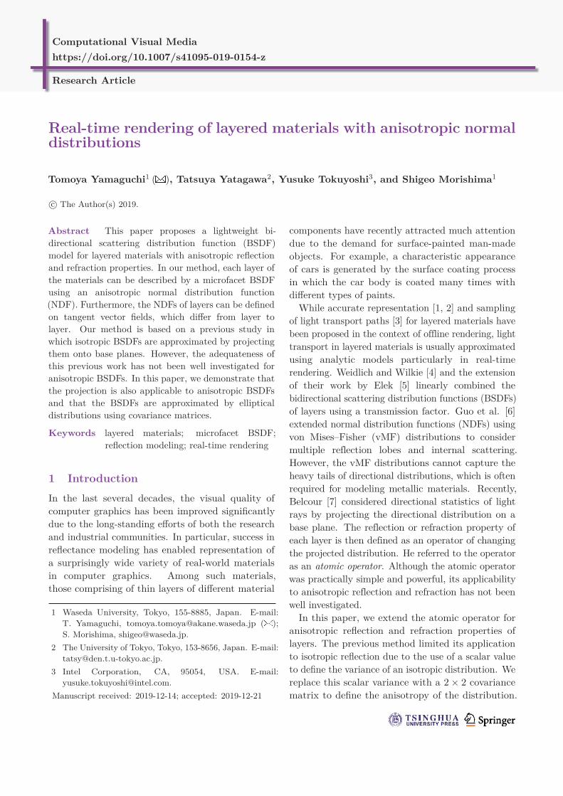
The proposed method is an extension of Belcour’smethod [7] which approximated BSDFs by projectingthem onto the base plane. The previous studyrestricted their applicability only to isotropic NDFs.In contrast, the proposed method extends theapproach to anisotropic NDFs, as shown in Fig. 1.

Real-time rendering of layered materials with anisotropic normal distributions 3

Fig. 1 Our method works for layers with anisotropic NDFs definedon varying tangent vector fields, whereas the previous method [7] canbe applied only to isotropic NDFs.

3.1 Covariance of projected distribution

To represent anisotropic BSDFs projected on thebase plane, we employ a 2 × 2 covariance matrixΣ rather than a scalar variance σ. However, therelationship between the tangent vector field andthe covariance matrix is non-trivial. Let tx ∈ S1

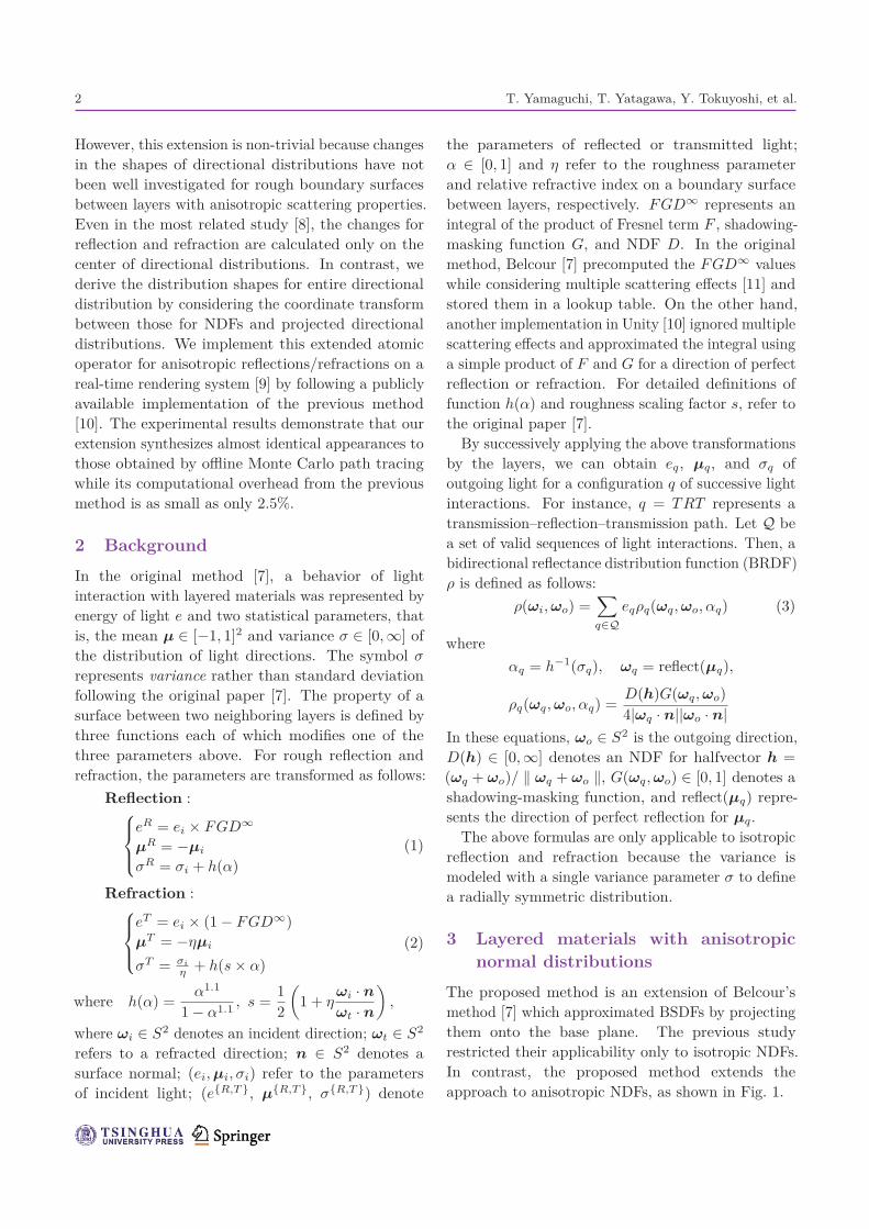
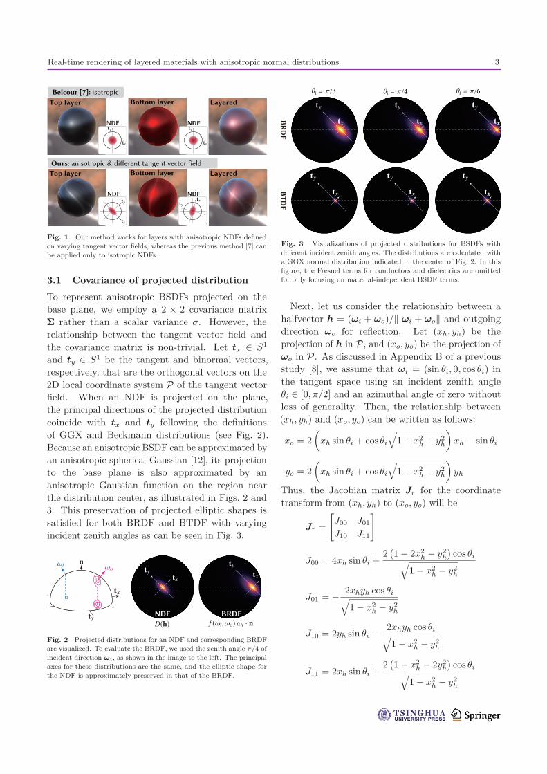
and ty ∈ S1 be the tangent and binormal vectors,respectively, that are the orthogonal vectors on the2D local coordinate system P of the tangent vectorfield. When an NDF is projected on the plane,the principal directions of the projected distributioncoincide with tx and ty following the definitionsof GGX and Beckmann distributions (see Fig. 2).Because an anisotropic BSDF can be approximated byan anisotropic spherical Gaussian [12], its projectionto the base plane is also approximated by ananisotropic Gaussian function on the region nearthe distribution center, as illustrated in Figs. 2 and3. This preservation of projected elliptic shapes issatisfied for both BRDF and BTDF with varyingincident zenith angles as can be seen in Fig. 3.

Fig. 2 Projected distributions for an NDF and corresponding BRDFare visualized. To evaluate the BRDF, we used the zenith angle π/4 ofincident direction ωi, as shown in the image to the left. The principalaxes for these distributions are the same, and the elliptic shape forthe NDF is approximately preserved in that of the BRDF.

Fig. 3 Visualizations of projected distributions for BSDFs withdifferent incident zenith angles. The distributions are calculated witha GGX normal distribution indicated in the center of Fig. 2. In thisfigure, the Fresnel terms for conductors and dielectrics are omittedfor only focusing on material-independent BSDF terms.

Next, let us consider the relationship between ahalfvector h = (ωi + ωo)/‖ ωi + ωo‖ and outgoingdirection ωo for reflection. Let (xh, yh) be theprojection of h in P, and (xo, yo) be the projection ofωo in P. As discussed in Appendix B of a previousstudy [8], we assume that ωi = (sin θi, 0, cos θi) inthe tangent space using an incident zenith angleθi ∈ [0, π/2] and an azimuthal angle of zero withoutloss of generality. Then, the relationship between(xh, yh) and (xo, yo) can be written as follows:

xo = 2(

xh sin θi + cos θi

√1 − x2

h − y2h

)xh − sin θi

yo = 2(

xh sin θi + cos θi

√1 − x2

h − y2h

)yh

Thus, the Jacobian matrix Jr for the coordinatetransform from (xh, yh) to (xo, yo) will be

Jr =[J00 J01

J10 J11

]

J00 = 4xh sin θi +2

(1 − 2x2

h − y2h

)cos θi√

1 − x2h − y2

h

J01 = − 2xhyh cos θi√1 − x2

h − y2h

J10 = 2yh sin θi − 2xhyh cos θi√1 − x2

h − y2h

J11 = 2xh sin θi +2

(1 − x2

h − 2y2h

)cos θi√

1 − x2h − y2

h

Bo�om layer

Bo�om layer Layered

LayeredTop layer

Top layer

NDF

NDF

NDF

NDF

Belcour [7]: isotropic

Ours: anisotropic & di�erent tangent vector field

BR

DF

BTD

F

NDF BRDF


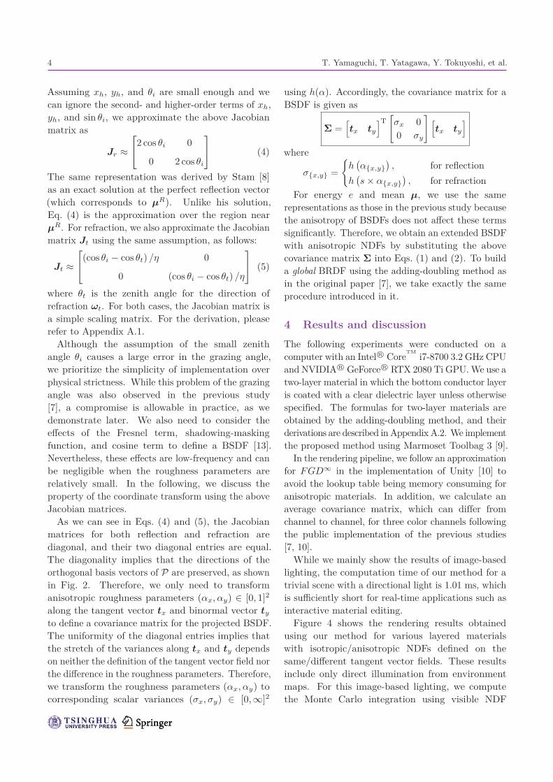
Assuming xh, yh, and θi are small enough and wecan ignore the second- and higher-order terms of xh,yh, and sin θi, we approximate the above Jacobianmatrix as

Jr ≈2 cos θi 0

0 2 cos θi

(4)

The same representation was derived by Stam [8]as an exact solution at the perfect reflection vector(which corresponds to µR). Unlike his solution,Eq. (4) is the approximation over the region nearµR. For refraction, we also approximate the Jacobianmatrix Jt using the same assumption, as follows:

Jt ≈(cos θi − cos θt) /η 0

0 (cos θi − cos θt) /η

(5)

where θt is the zenith angle for the direction ofrefraction ωt. For both cases, the Jacobian matrix isa simple scaling matrix. For the derivation, pleaserefer to Appendix A.1.

Although the assumption of the small zenithangle θi causes a large error in the grazing angle,we prioritize the simplicity of implementation overphysical strictness. While this problem of the grazingangle was also observed in the previous study[7], a compromise is allowable in practice, as wedemonstrate later. We also need to consider theeffects of the Fresnel term, shadowing-maskingfunction, and cosine term to define a BSDF [13].Nevertheless, these effects are low-frequency and canbe negligible when the roughness parameters arerelatively small. In the following, we discuss theproperty of the coordinate transform using the aboveJacobian matrices.

As we can see in Eqs. (4) and (5), the Jacobianmatrices for both reflection and refraction arediagonal, and their two diagonal entries are equal.The diagonality implies that the directions of theorthogonal basis vectors of P are preserved, as shownin Fig. 2. Therefore, we only need to transformanisotropic roughness parameters (αx, αy) ∈ [0, 1]2

along the tangent vector tx and binormal vector ty

to define a covariance matrix for the projected BSDF.The uniformity of the diagonal entries implies thatthe stretch of the variances along tx and ty dependson neither the definition of the tangent vector field northe difference in the roughness parameters. Therefore,we transform the roughness parameters (αx, αy) tocorresponding scalar variances (σx, σy) ∈ [0, ∞]2

using h(α). Accordingly, the covariance matrix for aBSDF is given as

Σ =[tx ty

]T[σx 00 σy

] [tx ty

]

where

σ{x,y} ={

h(α{x,y}

), for reflection

h(s × α{x,y}

), for refraction

For energy e and mean µ, we use the samerepresentations as those in the previous study becausethe anisotropy of BSDFs does not affect these termssignificantly. Therefore, we obtain an extended BSDFwith anisotropic NDFs by substituting the abovecovariance matrix Σ into Eqs. (1) and (2). To builda global BRDF using the adding-doubling method asin the original paper [7], we take exactly the sameprocedure introduced in it.

4 Results and discussionThe following experiments were conducted on acomputer with an Intel R© Core

TMi7-8700 3.2 GHz CPU

and NVIDIA R© GeForce R© RTX 2080 Ti GPU. We use atwo-layer material in which the bottom conductor layeris coated with a clear dielectric layer unless otherwisespecified. The formulas for two-layer materials areobtained by the adding-doubling method, and theirderivations are described in Appendix A.2. We implementthe proposed method using Marmoset Toolbag 3 [9].

In the rendering pipeline, we follow an approximationfor FGD∞ in the implementation of Unity [10] toavoid the lookup table being memory consuming foranisotropic materials. In addition, we calculate anaverage covariance matrix, which can differ fromchannel to channel, for three color channels followingthe public implementation of the previous studies[7, 10].

While we mainly show the results of image-basedlighting, the computation time of our method for atrivial scene with a directional light is 1.01 ms, whichis sufficiently short for real-time applications such asinteractive material editing.

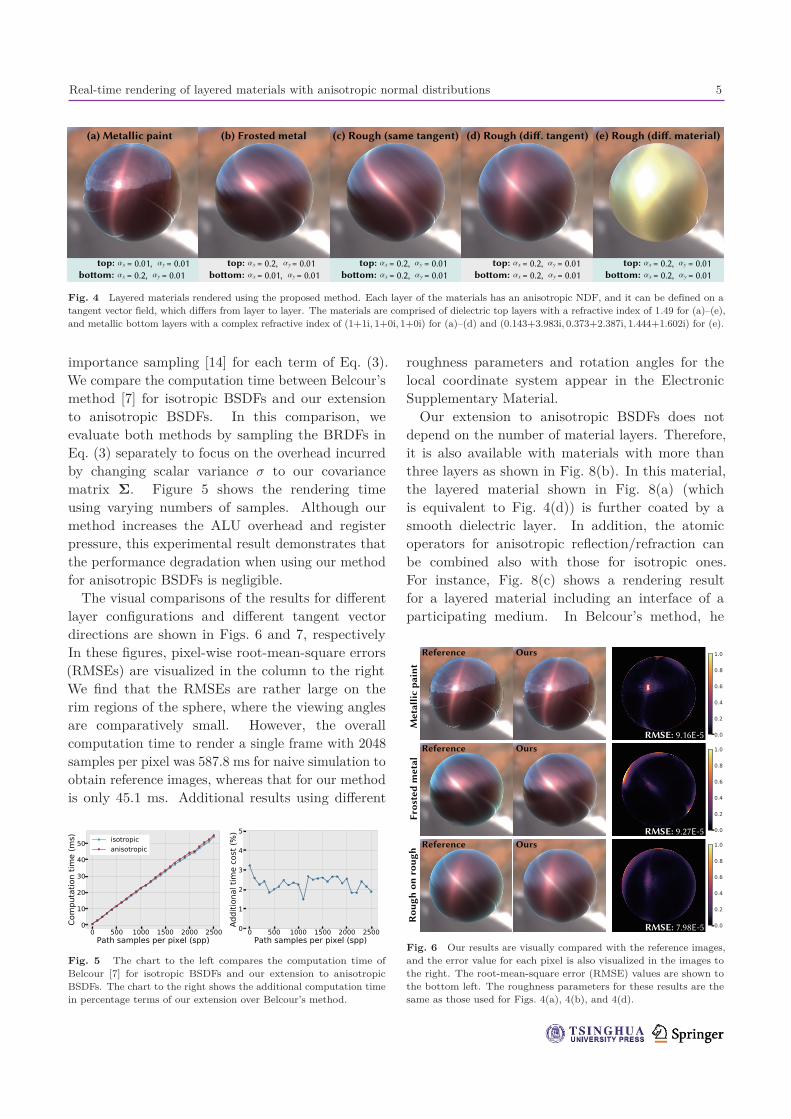
Figure 4 shows the rendering results obtainedusing our method for various layered materialswith isotropic/anisotropic NDFs defined on thesame/different tangent vector fields. These resultsinclude only direct illumination from environmentmaps. For this image-based lighting, we computethe Monte Carlo integration using visible NDF


Fig. 4 Layered materials rendered using the proposed method. Each layer of the materials has an anisotropic NDF, and it can be defined on atangent vector field, which differs from layer to layer. The materials are comprised of dielectric top layers with a refractive index of 1.49 for (a)–(e),and metallic bottom layers with a complex refractive index of (1+1i, 1+0i, 1+0i) for (a)–(d) and (0.143+3.983i, 0.373+2.387i, 1.444+1.602i) for (e).

importance sampling [14] for each term of Eq. (3).We compare the computation time between Belcour’smethod [7] for isotropic BSDFs and our extensionto anisotropic BSDFs. In this comparison, weevaluate both methods by sampling the BRDFs inEq. (3) separately to focus on the overhead incurredby changing scalar variance σ to our covariancematrix Σ. Figure 5 shows the rendering timeusing varying numbers of samples. Although ourmethod increases the ALU overhead and registerpressure, this experimental result demonstrates thatthe performance degradation when using our methodfor anisotropic BSDFs is negligible.

The visual comparisons of the results for differentlayer configurations and different tangent vectordirections are shown in Figs. 6 and 7, respectively.In these figures, pixel-wise root-mean-square errors(RMSEs) are visualized in the column to the right.We find that the RMSEs are rather large on therim regions of the sphere, where the viewing anglesare comparatively small. However, the overallcomputation time to render a single frame with 2048samples per pixel was 587.8 ms for naive simulation toobtain reference images, whereas that for our methodis only 45.1 ms. Additional results using different

Fig. 5 The chart to the left compares the computation time ofBelcour [7] for isotropic BSDFs and our extension to anisotropicBSDFs. The chart to the right shows the additional computation timein percentage terms of our extension over Belcour’s method.

roughness parameters and rotation angles for thelocal coordinate system appear in the ElectronicSupplementary Material.

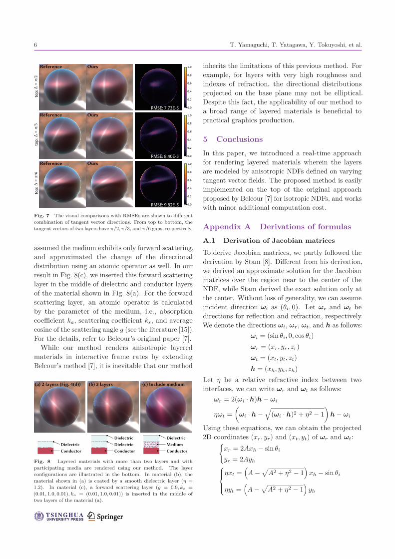
Our extension to anisotropic BSDFs does notdepend on the number of material layers. Therefore,it is also available with materials with more thanthree layers as shown in Fig. 8(b). In this material,the layered material shown in Fig. 8(a) (whichis equivalent to Fig. 4(d)) is further coated by asmooth dielectric layer. In addition, the atomicoperators for anisotropic reflection/refraction canbe combined also with those for isotropic ones.For instance, Fig. 8(c) shows a rendering resultfor a layered material including an interface of aparticipating medium. In Belcour’s method, he

Fig. 6 Our results are visually compared with the reference images,and the error value for each pixel is also visualized in the images tothe right. The root-mean-square error (RMSE) values are shown tothe bottom left. The roughness parameters for these results are thesame as those used for Figs. 4(a), 4(b), and 4(d).

(a) Metallic paint (b) Frosted metal (d) Rough (di�. tangent)(c) Rough (same tangent) (e) Rough (di�. material)

= 0.01, = 0.01top: = 0.2, = 0.01bo�om:

= 0.2, = 0.01top: = 0.01, = 0.01bo�om:

= 0.2, = 0.01top: = 0.2, = 0.01bo�om:

= 0.2, = 0.01top: = 0.2, = 0.01bo�om:

= 0.2, = 0.01top: = 0.2, = 0.01bo�om:

Met

allic

pai

ntFr

oste

d m

etal

Rou

gh o

n ro

ugh

RMSE: 9.16E-5

RMSE: 9.27E-5

RMSE: 7.98E-5

Reference Ours

Reference Ours

Reference Ours


Fig. 7 The visual comparisons with RMSEs are shown to differentcombination of tangent vector directions. From top to bottom, thetangent vectors of two layers have π/2, π/3, and π/6 gaps, respectively.

assumed the medium exhibits only forward scattering,and approximated the change of the directionaldistribution using an atomic operator as well. In ourresult in Fig. 8(c), we inserted this forward scatteringlayer in the middle of dielectric and conductor layersof the material shown in Fig. 8(a). For the forwardscattering layer, an atomic operator is calculatedby the parameter of the medium, i.e., absorptioncoefficient ka, scattering coefficient ks, and averagecosine of the scattering angle g (see the literature [15]).For the details, refer to Belcour’s original paper [7].

While our method renders anisotropic layeredmaterials in interactive frame rates by extendingBelcour’s method [7], it is inevitable that our method

Fig. 8 Layered materials with more than two layers and withparticipating media are rendered using our method. The layerconfigurations are illustrated in the bottom. In material (b), thematerial shown in (a) is coated by a smooth dielectric layer (η =1.2). In material (c), a forward scattering layer (g = 0.9, ks =(0.01, 1.0, 0.01), ka = (0.01, 1.0, 0.01)) is inserted in the middle oftwo layers of the material (a).

inherits the limitations of this previous method. Forexample, for layers with very high roughness andindexes of refraction, the directional distributionsprojected on the base plane may not be elliptical.Despite this fact, the applicability of our method toa broad range of layered materials is beneficial topractical graphics production.

5 ConclusionsIn this paper, we introduced a real-time approachfor rendering layered materials wherein the layersare modeled by anisotropic NDFs defined on varyingtangent vector fields. The proposed method is easilyimplemented on the top of the original approachproposed by Belcour [7] for isotropic NDFs, and workswith minor additional computation cost.

Appendix A Derivations of formulasA.1 Derivation of Jacobian matrices

To derive Jacobian matrices, we partly followed thederivation by Stam [8]. Different from his derivation,we derived an approximate solution for the Jacobianmatrices over the region near to the center of theNDF, while Stam derived the exact solution only atthe center. Without loss of generality, we can assumeincident direction ωi as (θi, 0). Let ωr and ωt bedirections for reflection and refraction, respectively.We denote the directions ωi, ωr, ωt, and h as follows:

ωi = (sin θi, 0, cos θi)ωr = (xr, yr, zr)ωt = (xt, yt, zt)h = (xh, yh, zh)

Let η be a relative refractive index between twointerfaces, we can write ωr and ωt as follows:

ωr = 2(ωi · h)h − ωi

ηωt =(

ωi · h −√

(ωi · h)2 + η2 − 1)

h − ωi

Using these equations, we can obtain the projected2D coordinates (xr, yr) and (xt, yt) of ωr and ωt:{

xr = 2Axh − sin θi

yr = 2Ayh

ηxt =(

A − √A2 + η2 − 1

)xh − sin θi

ηyt =(

A − √A2 + η2 − 1

)yh

RMSE: 9.16E-5

top:

RMSE: 7.73E-5

RMSE: 9.16E-5

top:

RMSE: 8.40E-5

RMSE: 9.16E-5

top:

RMSE: 9.82E-5

Reference Ours

Reference Ours

Reference Ours

DielectricConductor

DielectricDielectricConductor

DielectricMediumConductor

(a) 2 layers (Fig. 4(d)) (b) 3 layers (c) Include medium


where A = xh sin θi + cos θi

√1 − x2

h − y2h.

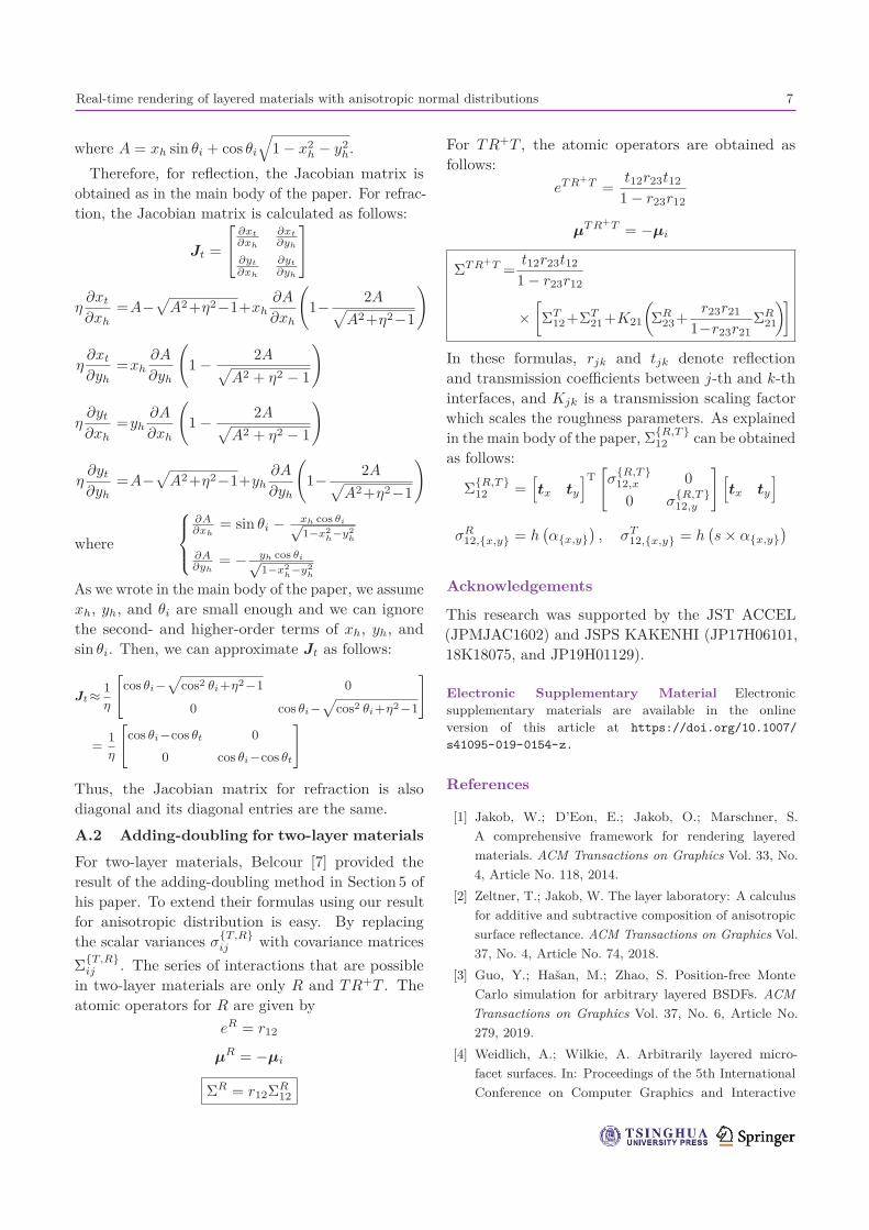
Therefore, for reflection, the Jacobian matrix isobtained as in the main body of the paper. For refrac-tion, the Jacobian matrix is calculated as follows:

Jt =

∂xt

∂xh

∂xt

∂yh

∂yt

∂xh

∂yt

∂yh

η∂xt

∂xh=A−

√A2+η2−1+xh

∂A

∂xh

(1− 2A√

A2+η2−1

)

η∂xt

∂yh=xh

∂A

∂yh

(1 − 2A√

A2 + η2 − 1

)

η∂yt

∂xh=yh

∂A

∂xh

(1 − 2A√

A2 + η2 − 1

)

η∂yt

∂yh=A−

√A2+η2−1+yh

∂A

∂yh

(1− 2A√

A2+η2−1

)

where

∂A∂xh

= sin θi − xh cos θi√1−x2

h−y2

h

∂A∂yh

= − yh cos θi√1−x2

h−y2

h

As we wrote in the main body of the paper, we assumexh, yh, and θi are small enough and we can ignorethe second- and higher-order terms of xh, yh, andsin θi. Then, we can approximate Jt as follows:

Jt ≈ 1η

[cos θi−

√cos2 θi+η2−1 0

0 cos θi−√

cos2 θi+η2−1

]

= 1η

[cos θi−cos θt 0

0 cos θi−cos θt

]

Thus, the Jacobian matrix for refraction is alsodiagonal and its diagonal entries are the same.

A.2 Adding-doubling for two-layer materials

For two-layer materials, Belcour [7] provided theresult of the adding-doubling method in Section 5 ofhis paper. To extend their formulas using our resultfor anisotropic distribution is easy. By replacingthe scalar variances σ

{T,R}ij with covariance matrices

Σ{T,R}ij . The series of interactions that are possible

in two-layer materials are only R and TR+T . Theatomic operators for R are given by

eR = r12

µR = −µi

ΣR = r12ΣR12

For TR+T , the atomic operators are obtained asfollows:

eT R+T =t12r23t12

1 − r23r12

µT R+T = −µi

ΣT R+T =t12r23t12

1 − r23r12

×[ΣT

12+ΣT21+K21

(ΣR

23+r23r21

1−r23r21ΣR

21

)]

In these formulas, rjk and tjk denote reflectionand transmission coefficients between j-th and k-thinterfaces, and Kjk is a transmission scaling factorwhich scales the roughness parameters. As explainedin the main body of the paper, Σ{R,T }

12 can be obtainedas follows:

Σ{R,T }12 =

[tx ty

]T[σ

{R,T }12,x 0

0 σ{R,T }12,y

] [tx ty

]

σR12,{x,y} = h

(α{x,y}

), σT

12,{x,y} = h(s × α{x,y}

)

Acknowledgements

This research was supported by the JST ACCEL(JPMJAC1602) and JSPS KAKENHI (JP17H06101,18K18075, and JP19H01129).

Electronic Supplementary Material Electronicsupplementary materials are available in the onlineversion of this article at https://doi.org/10.1007/s41095-019-0154-z.

References

[1] Jakob, W.; D’Eon, E.; Jakob, O.; Marschner, S.A comprehensive framework for rendering layeredmaterials. ACM Transactions on Graphics Vol. 33, No.4, Article No. 118, 2014.

[2] Zeltner, T.; Jakob, W. The layer laboratory: A calculusfor additive and subtractive composition of anisotropicsurface reflectance. ACM Transactions on Graphics Vol.37, No. 4, Article No. 74, 2018.

[3] Guo, Y.; Hasan, M.; Zhao, S. Position-free MonteCarlo simulation for arbitrary layered BSDFs. ACMTransactions on Graphics Vol. 37, No. 6, Article No.279, 2019.

[4] Weidlich, A.; Wilkie, A. Arbitrarily layered micro-facet surfaces. In: Proceedings of the 5th InternationalConference on Computer Graphics and Interactive


Techniques in Australia and Southeast Asia, 171–178,2007.

[5] Elek, O. Layered materials in real-time rendering. In:Proceedings of the 14th Central European Seminar onComputer Graphics, 2010.

[6] Guo, J.; Qian, J. H.; Guo, Y. W.; Pan, J. G.Rendering thin transparent layers with extendednormal distribution functions. IEEE Transactions onVisualization and Computer Graphics Vol. 23, No. 9,2108–2119, 2017.

[7] Belcour, L. Efficient rendering of layered materials usingan atomic decomposition with statistical operators.ACM Transactions on Graphics Vol. 37, No. 4, ArticleNo. 73, 2018.

[8] Stam, J. An illumination model for a skin layer boundedby rough surfaces. In: Rendering Techniques 2001.Gortler, S. J.; Myszkowski, K. Eds. Springer Vienna,39–52, 2001.

[9] Marmoset LLC. Marmoset Toolbag 3. 2019. Availableat https://marmoset.co/toolbag/.

[10] Unity Technologies. Unity Scriptable Render Pipeline.2019. Available at https://docs.unity3d.com/Manual/ScriptableRenderPipeline.html.

[11] Heitz, E.; Hanika, J.; D’Eon, E.; Dachsbacher, C.Multiple-scattering microfacet BSDFs with the Smithmodel. ACM Transactions on Graphics Vol. 35, No. 4,Article No. 58, 2016.

[12] Xu, K.; Sun, W.-L.; Dong, Z.; Zhao, D.-Y.; Wu, R.-D.; Hu, S.-M. Anisotropic spherical Gaussians. ACMTransactions on Graphics Vol. 32, No. 6, Article No.209, 2013.

[13] Walter, B.; Marschner, S.; Li, H.; Torrance, K.Microfacet models for refraction through rough surfaces.In: Proceedings of the 18th Eurographics Conferenceon Rendering Techniques, 195–206, 2007.

[14] Heitz, E. Sampling the GGX distribution of visiblenormals. Journal of Computer Graphics Techniques Vol.7, No. 4, 1–13, 2018.

[15] Henyey, L. C.; Greenstein, J. L. Diffuse radiation in theGalaxy. The Astrophysical Journal Vol. 93, 70–83, 1941.

Tomoya Yamaguchi is a masterstudent at Graduate School of AdvancedScience and Engineering, WasedaUniversity. He received his bachelorof engineering degree from WasedaUniversity in 2018. His research interestsinclude light transport algorithms andreal-time rendering.

Tatsuya Yatagawa is an assistantprofessor at School of Engineering, theUniversity of Tokyo. He received hisbachelor of science degree from KyotoUniversity in 2010 and received his Ph.D.degree from the University of Tokyo in2015. His research interests center oncomputer graphics and computer vision,

including efficient rendering, inverse rendering, and imageediting techniques.

Yusuke Tokuyoshi is a researchscientist at Intel Corporation. Beforejoining Intel, he engaged in R&D onrendering as a senior researcher atSQUARE ENIX CO., LTD. He receivedhis Ph.D. degree in engineering fromShinshu University in 2007. From 2007to 2010, he worked at Hitachi, Ltd. for

R&D on compiler optimization. His interests include globalillumination algorithms and real-time rendering.

Shigeo Morishima received his B.S.,M.S., and Ph.D. degrees in electricalengineering from the University of Tokyoin 1982, 1984, and 1987, respectively.Currently, he is a professor of Schoolof Advanced Science and Engineering,Waseda University. His research interestsinclude computer graphics, computer

vision, and human computer interaction. He is a trusteeof Japanese Academy of Facial Studies and a fellow of theInstitute of Image Electronics Engineers of Japan.

Open Access This article is licensed under a CreativeCommons Attribution 4.0 International License, whichpermits use, sharing, adaptation, distribution and reproduc-tion in any medium or format, as long as you give appropriatecredit to the original author(s) and the source, provide a linkto the Creative Commons licence, and indicate if changeswere made.

The images or other third party material in this article areincluded in the article’s Creative Commons licence, unlessindicated otherwise in a credit line to the material. If materialis not included in the article’s Creative Commons licence andyour intended use is not permitted by statutory regulation orexceeds the permitted use, you will need to obtain permissiondirectly from the copyright holder.

To view a copy of this licence, visit http://creativecommons.org/licenses/by/4.0/.

Other papers from this open access journal are availablefree of charge from http://www.springer.com/journal/41095.To submit a manuscript, please go to https://www.editorialmanager.com/cvmj.

Documents

Real-time rendering of layered materials with anisotropic