I / 3 0

ALIGNMENT OF TARN II

Akira Noda*, Morio Yoshizawa, Tamaki Watanabe, Toshiaki Osuka* *,Takeshi Katayama, Akird Mizobuchi

Institute for Nuclear Study, University of Tokyo, Midori-cho 3-2-1, Tanashi-city, Tokyo 188, Japan

Kazushi EmotoNihon Kensetsu Kogyo, Co., Ltd., ShinbashiS-13-11, Minato-ku, Tokyo 105, Japan

walls exist as shown in Fig. 1. So somedistances of the magnets from the center cannotbe measured. In order to keep the hexagonalshape of TARN II ring, special care is neededand algorithm to calculate the optimum positioncorrection to each magnet based onHouseholder’s method has been developed.Positioning holes whose positions are preciselycontrolled at the fabrication stage of the magnetare made on each magnet. The distancesbetween the positioning holes on the magnets andcenter pole are measured by a distometer utilizingInvar wires 1.0 mm in diameter (made by KernCo. Ltd.). The absolute value of the distance iscalibrated on a straight rail with use of a laserinterferometer (HP 5526A) at each measurement.The distometer measures the difference of thedistance to be measured from the known distanceon the calibration rails.

In the present paper, the algorithm of thepositioning of the magnets are given, then realalignment procedure is described together withthe final results of alignment of TARN II.

1. Introduction

TARN II is a heavy ion synchrotron/cooler ring, whose average radius and circumference are12.4 m and 77.8 m, respectively. Main parameters of TARN II are listed up in Table 1[1]. As theradius of curvature of dipole is 4.045 m and the deflection angle of each dipole magnet is I5 o, themethod to set the magnets on the equilateral triangles around the ring center is considered to be moreeffective compared with such a method as “perpendicular-short chord” or “short-long chord”measurement[2]. The ring is set in the experimental hall composed of three parts between which two

Fig. 1 Layout of TARN II.

*Present address: Institute for Chemical Research, Kyoto University**Present address: College of Arts and Sciences, Chiba University

I /31

2. Algorithm of the Alignment

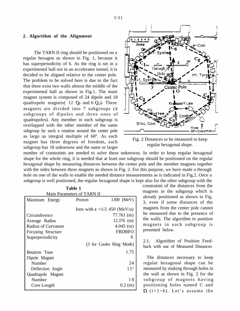
The TARN II ring should be positioned on aregular hexagon as shown in Fig. 1, because ithas superperiodicity of 6. As the ring is set in aexperimental hall not in an accelerator tunnel, it isdecided to be aligned relative to the center pole.The problem to be solved here is due to the factthat there exist two walls almost the middle of theexperimental hall as shown in Fig.1. The mainmagnet system is composed of 24 dipole and 18quadrupole magnets( 12 QF and 6 QD). Thesemagnets are divided into 7 subgroups (4subgroups of d ipoles and three ones ofquadrupoles). Any member in each subgroup isoverlapped with the other member of the samesubgroup by such a rotation around the center poleas large as integral multiple of 60º. As eachmagnet has three degrees of freedom, eachsubgroup has 18 unknowns and the same or larger

Fig. 2 Distances to be measured to keepregular hexagonal shape.

number of constraints are needed to solve these unknowns. In order to keep regular hexagonalshape for the whole ring, it is needed that at least one subgroup should be positioned on the regularhexagonal shape by measuring distances between the center pole and the member magnets togetherwith the sides between these magnets as shown in Fig. 2. For this purpose, we have made a throughhole on one of the walls to enable the needed distance measurements as is indicated in Fig.2. Once asubgroup is well positioned, the regular hexagonal shape is kept also for the other subgroup with the

Table 1Main Parameters of TARN II

Maximum Energy Proton 1300 (MeV)

Ions with E =1/2 450 (MeV/u)Circumference 77.761 (m)Average Radius 12.376 (m)Radius of Curvature 4.045 (m)Focusing Structure FBDBFOSuperperiodicity 6

(3 for Cooler Ring Mode)

Betatron Tune 1.75Dipole Magnet

Number 24Deflection Angle 15º

Quadrupole MagnetNumber 1 8Core Length 0.2 (m)

constraints of the distances from themagnets in the subgroup which isalready positioned as shown in Fig.3, even if some distances of themagnets from the center pole cannotbe measured due to the presence ofthe walls. The algorithm to positionmagnets in each subgroup ispresented below.

2.1. Algorithm of Position Feed-back with use of Measured Distances

The distances necessary to keepregular hexagonal shape can bemeasured by making through holes inthe wall as shown in Fig. 2 for thesubgroup o f magne t s hav ingpositioning holes named C andDi ( i=1~6) . Le t ’ s a s sume the

I / 3 2

Fig. 3 Constraints to keep the regular hexagonal shape Fig. 4 Definition of the possible positiononce a subgroup has been well aligned. Error of the ith member magnet.

displacements in the horizontal plane and the rotation of the i-th member magnet from the ideal positionto be Axi, Ayi and A8i, respectively as is indicated in Fig. 4. If we start the precise alignment afterprepositioning, then the displacements and rotation angle, Q, Ayi and AtI; can well be considered tobe small quantities and their higher order terms than second order can be neglected. Thus from the 23measured distances ofm , cici+l, D;u;,l (i=1, --,6) and m(i=l, --5), the following 23 constraintscan be obtained for 18 unknowns of displacements and rotations of the six magnets in the subgroup.

I / 3 3

where & is the fixed distance between the two positioning holes in the same dipole magnet (0.850 m)and 80 is the angle defined in Fig.4. OD6 cannot be measured due to the presence of structure pillar inthe wall. If we denote the coefficients of the left-hand sides of these equations to be Aij and the termsof right-hand sides to be b;, then these equations can be written as

wherexdenotes 18 dimensional vector composed of A&, Ayi and A8i (i=1,---,6) and A and b are the23x18 matrix and 18 dimensional vector, respectively. In order to obtain the 18 unknovvns. AXi, Ayiand Aei, which simultaneously satisfies 23 independent linear equations (l)~(4), which can berewritten as Eq. (5), the solution which minimizes the norm, /A?-bll is obtained with use of theScientific Subroutine (SSLII) utilizing Householder’s transformation, It is not obvious that thisalgorithm is valid for the present case, so we have made the check of the validity of this method bygenerating the random position errors utilizing pseudo-random number. For randomly generatedpositions of the six member magnets, distances among magnets and the distance of the magnets fromthe center pole can be calculated. Only using these distance data and using the algorithm abovementioned, the position errorsx( i.e. AX;, Ayi and Aei (i=1,---,6)) can be solved, which coincide withthe generated ones within 0.002 mm or 0.002 mrad, which is considered quite satisfactory.

For the other subgroups, it is not possible to measure all the distances of the member magnetsfrom the center pole. However, in this case we have added constraints by measuring the distancesfrom the nearby magnets which belong to the already positioned subgroup as indicated in Fig. 3. Soin this case, the following relations are added in addition to equations (l)~(4), where c and 0, arereplaced by a and Cl,, respectively although some of them will be missing due to presence of the walls.If we take the subgroup of magnets having positioning holes named -4; and Bi as an example, therelation can be written as

I / 3 4

where 8, and 0, are angles defined in Fig. 3. In the present example, m, OBi (i=2,--,5), AiAi+r,BiBi+l, m(i=l,--,6) are measured and total 26 constraints are imposed on 18 unknowns. In thiscase, the validity of the algorithm of Eq. (5) with 26x18 matrix A is also checked by generatedposition errors with use of pseudo-random number and is found that the position error can be solvedwithin 0.002 mm. For other subgroups, similar algorithm is used to align the member magnets.

2.2. Applied Position Feed-Back by the Measured Data

From the solution of simultaneous equation (5), the displacement from the ideal position, AXi,Ayi and A8i are obtained for each magnet. So the position feed back process is decomposed into thepositioning of each individual magnet. Real position correction needed for the magnet is calculated asfollows

with the notation given in Fig. 4.By observing the displacement of the magnet in the horizontal plane with use of dial gauges

attached to each side of the magnet, the position of the magnet can be well controlled.

3. Real Procedure of the Alignment

In the procedure of the alignment, all the magnets should be set horizontally with use of a waterlevel at first. The precision of the horizontal adjustment is better than 0.2 mrad. Then they are to be

set at the same height with the use of the auto levelwith an optical micrometer. Its minimum scale is0.1 mm and the precision of the median planeadjustment is better than ±0.1mm including theerror due to parallax.

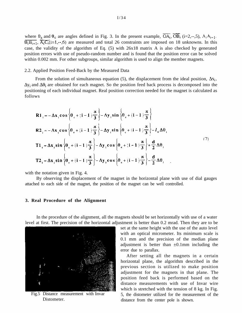
After setting all the magnets in a certainhorizontal plane, the algorithm described in theprevious section is utilized to make positionadjustment for the magnets in that plane. Theposition feed back is performed based on thedistance measurements with use of Invar wirewhich is stretched with the tension of 8 kg. In Fig.

Fig.5 Distance measurement with Invar 5, the distometer utilized for the measurement of theDistometer. distance from the center pole is shown.

I /35

As the distometer only measures the differenceof the distance from the one already known set on astraight rail for the calibration purpose, the absolutevalue of the distance is calibrated with use of laserlinear interferometer (HP5526A). At the present case,the distances between magnets in the same subgroupand the distances of the magnets from the center poleare ~12 m, the length change amounts to the order of0.06 mm if the temperature change is 5°C even for thecase of Invar wire with the expansion coefficient of theorder of 106. As the experimental hall has no air-conditioning, the distance measurement was performedalmost similar time in the day and the absolute length iscalibrated at every measurement. In Fig. 6, the lengthcalibration process on the straight rail is shown.

Fig. 6 Absolute Length Calibration withLaser Interferometer.

The precise alignment is started after the pre-positioning with the precision better than ±10mm.With the use of algorithm given in 2.1, the estimated position errors of all the magnets became lessthan -1 mm after twice iterations. In Fig.7, position deviations of the member magnets after theseiterations are shown for the case of alignment of subgroup with alignment holes l!$ and Fi as anexample. From the results, the convergence of the algorithm seems quite nice.

However, the alignment process stagnated after the position deviations of the magnets becameless than 0.5 mm. At first the stiffness of the girder was suspected and the motion of the magnet afterposition correction was monitored whole night with dial gauges attached to the pillars fixed to the

Fig. 7 Position deviations of magnets in subgroup (E,F) after pre-positioning, and the first andsecond iterations of the position feed back.

I/36

floor. However no noticeable movement was found. Finally after making measurements without anyposition correction, it was found that the floor moved non uniformly day by day with the order of afew hundreds pm as shown in Fig. 8. The global changes are consistent with the thermal expansioncoefficient of concrete and we can avoid them by temperature correction. However, the nonhomologous change as shown in m cannot be corrected. So it was decided to terminate thealignment process with the precision of ±0.4 mm. In Table 2, the final deviations of measured

Table 2Deviations of the finally measured distances from the ideal ones (mm).

I / 3 7

Fig. 8 Daily Variation of distances withoutPosition Correction.

distances from the ideal ones arelisted up. In Table 3, the estimatedclosed orbit distortion is given forthe case of position precision of±0.4 mm together with ±0.1 mmcase. From the table, the root meansquare sum of the closed orbitdistortion seemed to be not so muchdifferent and the running in ofTARN II was started under thisc o n d i t i o n , w h i c h w a s v e r ysucces s fu l ly pe r fo rmed [1 ] .Without any orbit correction, thec l o s e d o r b i t d i s t o r t i o n w a smeasured to be a little bit smaller(less than 10mm and 6 mm inhorizontal and vertical directions,respectively) than the estimationgiven in Table 3, which wascorrected with use of theelectrostatic position pick-ups withhigh sensitivity and correction coilswound on the dipole magnets orvertical steering magnets[3] and the

closed orbit distortion is reduced less than 1 mm as shown in Fig. 9[4]. Thus the present method ofthe alignment seems to have worked well although some difficulty existed to keep the precision of±0.1mm originally aimed at due to the non uniform movement of the floor, because the experimentalhall was made of three different parts made at the different times and on the different bases.

Acknowledgements

The authors would like to present their sincere thanks to Prof. Y. Hirao for his continuousencouragement during the work. They are very grateful to Prof. K. Endo at KEK for his fruitfuldiscussion about alignment of magnets for synchrotron ring and also his aids to lend us the Invardistometer during the present alignment process. Their thanks are also due to other members ofaccelerator division of INS who collaborated on TARN II. Cooperation of Nihon Kensetsu Kogyo isalso greatly appreciated.

REFERENCES

[1] T. Katayama, “Cooler Synchrotron TARN II, Present and Future”, Proceedings of the 19th INSSymposium, COOLER RINGS AND THEIR APPLICATIONS, Tokyo, Japan (1990) pp21-30.

[2] K. Endo and M. Kihara, “Precise Alignment of Magnets around Accelerator Ring”, KEK Report,KEK-74-3 (1974).

[3] T. Tanabe et al., “Vertical COD Correction”, Institute for Nuclear Study, University of Tokyo,Annual Report 1992, p120.

[4] T. Watanabe et al., “Beam Position Monitoring System and C.O.D. Correction at the CoolerSynchrotron TARN II”, to be submitted to Nuclear Instrument and Methods.

I / 3 8

Table 3Closed Orbit Distortion

Horizontal Direction Vertical Direction

Fig. 9 (a) Closed Orbit Distortion without Orbit Correction.

Horizontal Direction Vertical Direction

Fig. 9 (b) Closed Orbit Distortion with Orbit Correction.