Embed Size (px)
Citation preview

- i -
Methods for Knowledge Discovery in
Data
University of Seville
Department of Languages and
Information Systems
Dissertation submitted in partial fulfilment of the requirements for the degree of Doctor Europeo en Informática, presented by
Santiago Patricio Serendero Sáez
Advisor: Professor José Miguel Toro Bonilla
June, 2004

ii
The more perfect a nature is the fewer means it requires for its operation.
Aristotle's
All exact science is dominated by the idea of approximation
Bertrand Russell

iii
Agradecimientos
Agradezco muy sinceramente la ayuda prestada por mi Director de Tesis, Prof. Dr.
Miguel Toro durante todos estos años. Su contribución ha sido fundamental en la
formalización de los algoritmos de este trabajo.
Agradezco a Erika y Andrea, cuyo amor ha sido la energía elemental que ayudó a
mantener este barco contra viento y marea. Sin ellas este trabajo no habría podido ser.
Agradezco a mis padres, que me dieron los materiales esenciales para la culminación
exitosa de esta fase de mi vida, y que aquí y Allá se están todavía preguntando en que
cosas he andado metido todo este tiempo.
Agradezco a amigos y colegas que me han ayudado. A los colegas R. Martínez de la
U. de Sevilla , H. Shahbazkia y Fernando Lobo de la U. de Algarve, por la gentileza que
tuvieron de leer el manuscrito original y hacerme valiosas críticas. A G. Oliveira e A.
Jones por su corrección del manuscrito en Inglés. A J. Lima, por su ayuda en la revisión
de algunos algoritmos. A T. Boski, por su aliento permanente. A F. Saravia y a María
Pía Labbé por su entusiasta apoyo desde mi distante y querido Chile.
Una palabra especial de agradecimiento a los colegas del Departamento de Lenguajes
y Sistemas de la Universidad de Sevilla. Me han tratado de tal modo, que en todo
momento me he sentido allí como en mi tierra.
Parte del tiempo de trabajo de esta tesis, ha sido hecho con el apoyo del programa de
acción 5.2 PRODEP financiado por la Unión Europea.

- iv -
Abstract
This thesis contributes to the development of tools for Supervised Learning, and in
particular for the purposes of classification and prediction, a problem of interest to
everyone working with data.
After analysing some of the most typical problems found in instance-based and
decision trees methods, we develop some algorithmic extensions to some of the most
critical areas found in the process of Data Mining when these methods are used.
We begin by studying sampling data and the benefits of stratified data composition in
the training and test evaluations sets. We study next the characteristics and degree of
relevance of attributes, a problem of paramount importance in data mining. We do this
by means of identifying the discriminatory power of attributes with respect to classes.
Selecting most relevant attributes increases algorithm complexity, which is exponential
in the number of attributes. For this reason, verifying every other possible subset of
candidate attributes is sometimes out of question. In this respect, we provide a low-
complexity algorithm to help discover which attributes are relevant and which are not
[Serendero et al., 2003]. This technique forms an integral part of the classification
algorithm, and it could be utilised by rule induction algorithms using trees, as well as
instance-based methods using distance metrics for the application of the principle of
proximity.
In most instance-based methods, vector records relate to a class as a whole, i.e., each
record considered on its integrity relates to one class. The same idea is present in
decision trees, and for that reason classes appear only at tree leaves. On the contrary,
our algorithm relates class membership to cell prefixes, allowing a complete and new
approximation of sub-cell component elements to class membership. This concept is a
fundamental part of our algorithm.
Most instance based methods, and in particular, k-NN methods deal with the problem
of searching similar records to some unseen object in the data hyperspace based on
distance metrics. Selecting “close” neighbour objects from the hyperspace can be a
computationally expensive process. We contribute in this respect by offering a search
mechanism based on a tree structure with a low complexity cost and where the distance
calculation considers first attributes that are more relevant.

v
Selecting best neighbours of representative patterns not only depends on the
proximity of similar objects. We define several selection criteria weighted according
with data characteristics, thus adapting the algorithm to different data.
For all experiments, we present a comparison of results from two different sources,
namely results from the literature and results obtained in our own hardware using a
relatively new benchmark tool. This way is possible to keep equal testing conditions, a
condition difficult to find in figures from the literature.

vi
Contents
Agradecimientos.........................................................................................................iii
Abstract....................................................................................................................... iv
Contents ...................................................................................................................... vi
List of Tables .............................................................................................................. xi
List of Figures........................................................................................................... xiv
1 Introduction......................................................................................................... 1
1.1 Motivation for this thesis. Some background...................................................... 4
1.2 Instance-based and Decision Tree methods........................................................ 6
1.2.3.1 Problems with Decision Trees .................................................................. 8
1.2.3.2 Problems with Instance-based methods .................................................... 9
1.3 Objectives.......................................................................................................... 10
1.4 Contributions of this thesis ............................................................................... 11
1.5 Structure of this text .......................................................................................... 12
2 State-of-the-Art ................................................................................................. 15
2.1 Active areas of research and new challenges and directions ........................... 16
2.1.1 Active learning (AI)/experimental design (ED)......................................... 16
2.1.2. Cumulative learning.................................................................................. 17
2.1.3. Multitask learning ..................................................................................... 17
2.1.4. Learning from labelled and unlabeled data............................................... 17
2.1.5 Relational learning ..................................................................................... 17
2.1.6 Learning from huge datasets ...................................................................... 18
2.1.7 Learning from extremely small datasets .................................................... 18

vii
2.1.8 Learning with prior knowledge.................................................................. 18
2.1.9 Learning from mixed media data ............................................................... 18
2.1.10 Learning causal relationships................................................................... 19
2.1.11 Visualization and interactive data mining................................................ 19
2.2 General trends................................................................................................... 19
2.3 Different Perspectives of Data Mining ............................................................. 22
2.4 Similarity searching in tries.............................................................................. 25
2.4.1 Similarity searching metric spaces............................................................. 26
2.4.2 Some concepts for a metric space .............................................................. 26
2.4.3 Types of search .......................................................................................... 30
2.4.4 Equivalence relations ................................................................................. 31
2.5 Searching in tries .............................................................................................. 32
2.6 Data Mining and Statistical Sampling .............................................................. 35
2.6.1 Random sampling ...................................................................................... 35
2.6.1.1 Holdout method....................................................................................... 36
2.6.1.2 Cross-validation method ......................................................................... 37
2.6.1.3 Leave one out method ............................................................................. 38
2.6.1.4 Bootstrap method ................................................................................... 38
3 The Trie-Class Algorithm. Basic definitions .................................................. 39
3.1 General overview of the algorithm ................................................................... 39
3.2 Basic definitions................................................................................................ 40
3.3 Definitions on cell discretization ...................................................................... 41
3.4 Exclusiveness as a measure of attribute relevance........................................... 47
3.5 Attribute selection ............................................................................................. 49
3.6 Shape definitions ............................................................................................... 50
3.7 Searching for nearest cells................................................................................ 55
3.7.1 Selecting closest pattern............................................................................. 57
3.7.2 Using look-ahead to solve ties in cell pattern selection ............................. 59

viii
3.7.3 The search algorithm in practice ................................................................ 60
3.8 Extraction of p1 is an efficient alternative to regular k-NN methods................ 61
3.9 General assumptions on some basic Principles................................................ 63
3.9.1 Data consistency ........................................................................................ 63
3.9.2 Partition granularity ................................................................................... 64
3.9.3 Class membership, Patterns and the Continuity Principle ......................... 64
4 Pre-processing Data Before Mining ................................................................ 67
4.1 Converting records into discretized patterns.................................................... 67
4.2 The special case of categorical attributes......................................................... 69
4.3 Feature reduction and elimination ................................................................... 73
4.3.1 Ordering attributes ..................................................................................... 75
4.3.2 Looking at sub-cells from the “clearest” viewpoint................................... 75
4.3.3 Reducing attribute numbers ....................................................................... 77
5 Evaluation and Results..................................................................................... 81
5.1 Data used in experiments .................................................................................. 81
5.1.1 Adult dataset. (Census USA 1994)................................................................. 81
5.1.2 Annealing dataset ....................................................................................... 82
5.1.3 Breast Cancer (Wisconsin) dataset ............................................................ 82
5.1.4 Dermatology dataset .................................................................................. 83
5.1.5 Diabetes (Pima Indian) dataset .................................................................. 83
5.1.6 Forest Cover type dataset ........................................................................... 83
5.1.7 Heart disease dataset (Cleveland). ............................................................. 84
5.1.8 Heart disease Statlog.................................................................................. 84
5.1.9 Hypothyroid dataset ................................................................................... 85
5.1.10 Iris dataset ................................................................................................ 85
5.1.11 Pen-Based Recognition of Handwritten Digits: “pendigits” dataset ....... 85
5.1.12 Satellite image dataset (STATLOG version) ........................................... 86
5.1.13 German credit dataset............................................................................... 87

ix
5.2 The evaluation method used by Trie-Class ....................................................... 87
5.3 Comparison of results with other classifiers..................................................... 89
5.3.1 Results using figures from the bibliography.............................................. 89
5.3.2 Results from experiments done in our own hardware................................ 96
5.4 Performance Conclusions ............................................................................... 100
6 Choosing the best close neighbour ................................................................ 103
6.1 Decision parameters ....................................................................................... 105
6.1.1 Semi-exclusive values.............................................................................. 105
6.1.2 Distance between selected cells ............................................................... 105
6.1.3 The shape of cells..................................................................................... 106
6.1.4 Cell strength ............................................................................................. 106
6.1.5 Frequency of cells and sub-cells .............................................................. 107
6.1.6 The Majority Class................................................................................... 108
6.2 Basic functions definitions for the selection of a representative cell’s class.. 108
6.3 Obtaining the weight of decision parameters ................................................. 110
6.4 Predicting the final output class ..................................................................... 115
7 Implementation ............................................................................................... 119
7.1 General overview ............................................................................................ 119
7.2 Building a trie as the main tree structure ....................................................... 121
7.3 Insertion algorithm ......................................................................................... 125
7.4 Discussion on the actual implementation ....................................................... 126
7.5 Dictionary and other supporting files............................................................. 129
8 Conclusions and Future work........................................................................ 131
8.1 Conclusions..................................................................................................... 132
8.2 Future work..................................................................................................... 135

x
9 Bibliography .................................................................................................... 137
Appendix I. Example of Dictionary corresponding to the Annealing Dataset 153
Appendix II. Settings for the execution of the Naive Bayes classifier ............... 155
Appendix III. Alpha values for Decision Parameters ....................................... 159

xi
List of Tables
Table 2.1 Accepted papers in Data Mining and Machine Learning in four
International Congresses during 2002. ....................................................................... 21
Table 3.1 Attributes degree of relevance values in Cancer dataset...................... 50
Table 3.2 Cell vectors and their component values................................................ 53
Table 3.3 Shape vectors corresponding to cells from Table 3.2............................ 53
Table 3.4 Shape distances and similarity function values ..................................... 54
Table 3.5 Distance comparison using selected criteria .......................................... 55
Table 3.6 Original search space P containing 5 cells and a new query................ 60
Table 3.7 Classification error rates comparing p1 and IBk algorithm................. 62
Table 4.1 Class distributions by value for a symbolic attribute ........................... 73
Table 4.3 Variation in predictive error rate after ordering and reduction in the
number of attributes ..................................................................................................... 79
Table 5.1 Stratified sample characteristics in forest covert dataset..................... 89
Table 5.2 Adult dataset: Error Rate in predictive models .................................... 91
Table 5.3 Annealing dataset: Error Rate in predictive models ............................ 91
Table 5.4 Wisconsin Breast Cancer: Error Rate in predictive models ................ 92
Table 5.5 Dermatology dataset: Error Rate in predictive models........................ 92

xii
Table 5.6 Pima Indian Diabetes: Error Rate in predictive models ...................... 92
Table 5.7 Forest cover: Error Rate in predictive models ...................................... 93
Table 5.8 Heart disease, Cleveland: Error Rate in predictive models ................. 93
Table 5.9 Statlog Heart disease: Error Rate in predictive models ....................... 94
Table 5.10 Hypothyroid dataset: Error Rate in predictive models ..................... 94
Table 5.11 Iris dataset: Error Rate in predictive models ...................................... 95
Table 5.12 Pendigits dataset: Error Rate in predictive models ........................... 95
Table 5.13 Satellite image dataset (STATLOG): Error Rate in predictive models
95
Table 5.14 German Credit dataset. Error Rate in predictive models .................. 96
Table 5.15 Comparison in Classifiers accuracy using Weka against Trie-Class 98
Table 5.16 Comparing C 4.5 Error Rates from two sources................................. 99
Table 5.17 Classifiers execution total time for each individual fold using Weka.
100
Table 5.18 Error Rate comparison between Trie-Class, k-NN and two versions of
C4.5 100
Table 6.1 Function criterion return values by DP ............................................... 109
Table 6.2 Ambit and Precision values for decision parameters in various datasets
112

xiii
Table 6.3 Decision parameters weights for different datasets ............................ 114
Table. 7.1 Pseudo-code for insertion algorithm ................................................... 126
Table A-1 Weights (alpha) for various ambit and precision values expressed in
percentage.................................................................................................................... 159

xiv
List of Figures
Fig. 2.1 Different contours for constant Manhattan, Euclidean, L6, L � infinity
and Mahalanobis metrics in 2D space....................................................................... 29
Fig. 3.1 Attribute values projection in one-dimension to depict its relevance..... 49
Fig. 3.2 Slope intersection form of a line................................................................. 51
Fig. 3.3 A two-dimensional representation of a cell ............................................... 52
Fig. 3.4 Shape representation of six cell vectors..................................................... 54
Fig. 3.5 Searching for close neighbours................................................................... 61
Fig. 4.1 Different views on the same set of solutions.............................................. 76
Fig. 5.1. Flowchart for training and test sample subset selection......................... 89
Fig 6.1 Function apply() returns true if a criterion applies to a given cell ......... 110
Fig 6.2 Function predictr() predicts the label of a given record ......................... 111
Fig 6.4 Function that predicts the label class for a new query px. ...................... 117
Fig 7.1 Trie-Class main modules ........................................................................... 119
Fig. 7.2 Example of a classical trie after insertion of words................................ 122
Fig. 7.3 Section of C-trie showing 3 equal domain attribute levels ..................... 122
Fig. 7.4 Overlapped class regions in a two-dimensional space............................ 124

xv
Fig. 7.5 Overlap class regions in the hyperspace.................................................. 125


- 1 -
1 Introduction
The most important goal of handling data and performing computation is the
discovery of knowledge. We store data about a certain process and retrieve later that
information in order to use it in a meaningful way. To put it in the words of R. W.
Hamming, the purpose of computing is insight, not numbers. [Hamming, 1973]
Getting insight from small or moderate amounts of data was manageable until
recently. However, data collection with today’s computer technology has had such an
increment in volume in the last years that represents an explosion overwhelming all
expectations. According to a recent study “ The world produces between 1 and 2
exabytes1 of unique information per year, which is roughly 250 megabytes for every
man, woman, and child on earth.” …”It’s taken the entire history of humanity through
1999 to accumulate 12 exabytes of information. By the middle of 2002 the second dozen
exabytes will have been created”. In the conclusion of the same report, its authors say:
“ It is clear that we are all drowning in a sea of information. The challenge is to learn to
swim in that sea, rather than drown in it. Better understanding and better tools are
desperately needed if we are to take full advantage of the ever-increasing supply of
information”[Lyman, 2000].
These huge amounts of information do not only represent a challenging data
warehousing problem. In the last forty years database technology and disk capacity has
allowed the easy storage, manipulation and fast retrieval of ever growing volumes of
data, which is at the heart of today’s information society. However, much of this
increased power is wasted because humans are poor at gaining insight from data
presented in numerical form. When a database stores measurements, events, dates or
simply numbers, queries on that database return facts. Facts however are not exactly
knowledge, in the sense of concepts representing generalizations about data relations.
These concepts are the ones permitting the learning process to take place, by improving
our performance in an environment.
Congruent with the above indicated data production of the last years, the increase in
database size as well as the ever growing high dimension of records has dramatically

1 Introduction
2
expressed the idea that besides other relations than the ones defined a priori by database
designers, there was knowledge which could be extracted from databases. Moreover,
this knowledge would be crucial in the decision-making process.
With this premise in mind, the field has had a tremendous impact primarily on
industry wanting to take advantage of this hidden knowledge. The globalisation of
information through the Internet and the establishment of the e-business have increased
the need for tools and methods to elaborate knowledge from data produced massively
every second.
At the same time, the size of the problem made also clear that looking for knowledge
through tedious manual queries on large databases would have to be replaced by
advance computer algorithms running on faster hardware, as the sole possible solution.
It is within the goal of addressing these challenging issues that has taken place the
development of the area of Knowledge Discovery (KDD). Although inherently
associated with the area of databases for they contain the raw material for the
elaboration of knowledge, KDD is at the confluence of other research areas as well,
such as statistics, machine learning, pattern recognition, neural networks, rough and
fuzzy sets among others.
KDD is all of them and none of them. It is all of them, because the discipline jointly
uses techniques from several of these areas in order to attack the old problem of finding
patterns in data. It is none of them, because it is something more than the simple joint
utilization of these techniques developing its own methods, data structures and
algorithms. The reason for this development came as a realization that in solving
problems, which involve thousands of high dimensional records, no single method
could be expected to work well in the face of such diversity of data.
The term Knowledge Discovery appeared around 1989 and was defined as:
“...The nontrivial process of identifying valid, novel, potentially useful, and ultimately
understandable patterns in data” [Frawley et al., 1991].
However, the name popularising the field has been Data Mining, mostly used in the
economic and financial spheres. Later, the name was extended to Knowledge Discovery
1 An exabyte is a billion gigabytes or 1018 bytes.

1 Introduction
3
in Databases or KDD [Fayyad et al., 1995] to refer to the whole process, reserving the
name Data Mining only for the central inductive task2.
For these late authors, KDD is:
“The process of using the database along with any required selection, pre-
processing, sub-sampling, and transformations of it; to apply data mining methods
(algorithms) to enumerate patterns from it; and to evaluate the products of data mining
to identify the subset of the enumerated patterns deemed ‘knowledge’”.
In general, there are three main steps in the Knowledge Discovery process. First,
target data needs to be selected whether at a raw state or already in database format. At
this pre-processing stage, data is normalized and clean. A decision needs to be made on
what to do with records exhibiting missing data or data that seems to be in error. It is
also required at this stage to deal with the various types which data can present, in
particular its domain size, ordering, boundary values, etc.
Second, a phase recognized as Data Mining, which is the central inductive process of
pattern extraction. Inductive means obtaining knowledge through the inference of a new
theory from a set of observations, which is the experience. At this stage and depending
on the method been used, global or local hypotheses are created capturing the existing
relations in patterns of data under analysis.
Third, knowledge can be extracted from the obtained patterns. However, the resulting
information is not always in an easily interpretable form. For this reason, pattern
information and relations found must be put in a textual, graphical or visual form which
is more intelligible, such that can be understood and therefore useful to the expert
domain. Still the users of the data mining process must use the resulting knowledge.
They have to determine whether the accuracy of the results, the understandability of the
extracted knowledge, the time span to produce results and its practicality is useful or not
for them, establishing new goals. Generally, at this stage, the process reiterates again to
approximate to new objectives such as improving results, simplifying already obtained
knowledge or improving its visual representation.
2 In the context of this work we used indistinctively both expressions.

1 Introduction
4
In all these three phases, the interaction between the domain expert and the
programmer is required several times. Data and its meaning is not known by the
programmer. It is the domain expert experience and knowledge, which facilitates the
work of the programmer. For knowledge always can use previous knowledge about a
domain to generate a picture closer to reality. Furthermore, algorithm development and
resulting performance are data dependent. Therefore, choosing existing or designing
new algorithms requires the programmer expertise. In many cases, the parameters used
to produce hypotheses about data need to be changed dynamically as a function of data
and the algorithm itself. Interaction between the expert of the domain and the
programmer is again required. Finally, yet important, at the very end of one iteration
cycle within this process, is the decision of the data owner to accept or not the results
produced and offered by the programmer.
1.1 Motivation for this thesis. Some background
This thesis is about Data Mining and its related field Machine Learning (ML), itself a
sub-field of Artificial Intelligence. ML is the scientific field studying how machines can
learn, which is one of the components of intelligence. [Langley, 1996] proposes the
following definition of learning:
“Learning is the improvement of performance in some environment through the
acquisition of knowledge resulting from experience in that environment”
Both ML and Data Mining depend heavily on inductive reasoning, i.e. the reasoning
from particular observations available to the researcher leading to general concepts or
rules.

1 Introduction
5
Example 1 The following are examples of inductive reasoning and learning:
A tennis player trying to hit a forehand shot, will spend hundreds of shots learning
how to hit the ball in order to send it through the net at the desire height, speed and
direction, in order to place it far from the reach of his/her opponent. After 1000 shots,
he/she will have (hopefully) learned how to hit the ball appropriately. The knowledge
extracted from all those patterns describing the ball trajectory and place of impact, will
be then used the following time a similar shot is hit.
Someone concerned with the lack of water for human needs could measure over a
period of a year the amount of water wasted in a typical family home. This is the
experience. After observing many patterns of water consumption, this information could
be processed to demonstrate that 60% of that water contains only soap, 20% contains
other polluters and the remainder 20% contains other organic matter. This is the
knowledge. Using this knowledge in order to build houses with simple filter systems to
recycle a scarce resource such as water would mean that we have learned something.
In the context of this work, we deal only with the first subtask of the learning process,
namely the methods to acquire knowledge including the first two phases of knowledge
discovery referred to above.
Knowledge has to be extracted from data. Most of the time, we found data on its
original raw state, normally requiring a pre-process phase in order to be useful. Data has
to be clean, ordered, complete and consistent. Let us accept for the time being, that data
is ready to be processed. Records (examples, observations, objects) are usually
presented to the programmer as a sequence of vectors formed by Attribute values of
various data types. They represent the independent variables, with various degrees of
correlations between them. These attributes can be associated or not with a given label
or class, representing the dependent variable. Thus, a typical representation is the
following:
1 1 2 2| , | ,.., | ,.., | ,i i n nr A a A a A a A a c= (1.1)
We find an ordered sequence of the pair Attribute/value and optionally a
corresponding class, a symbol representing one among a finite discrete set of values.

1 Introduction
6
Depending on the presence or absence of the class, two classical problems constitute
a central goal in Data Mining. If the class is present in the available data, the goal can be
class prediction. If there is no input of classes, the goal will be clustering: to find natural
groupings or clusters of records in order to characterize data.
In the first case, learning from examples with or without a known class is called
Supervised Learning in Machine Learning taxonomy. Its goal is to obtain relevant data
patterns from available examples. These in turn will be used to generate general or local
hypotheses representing knowledge. This knowledge is used later to predict the class for
new unseen data. This process, which organizes data into a number of predetermined
categories, is called Classification. Classification is an uncertain task by nature, aiming
at making an educated guess about the value of the dependent variable class, based on
the value of the independent variables represented by attribute values. When the
submitted examples do not exhibit class membership, and the original database has
some natural cluster structure, a clustering algorithm must be first run, in order to make
explicit to each example its associated class label. The classification algorithm can be
executed after this.
When no prior data is available for learning, we are in the world of Unsupervised
Learning or Learning from Observation. The system must discover by itself its class
membership. To do that, it must first characterize common properties and behaviour of
examples forming clusters of records. The idea is to create groups of records with the
smallest possible differences among their members and the largest possible differences
between groups. This task has no prediction to make but to discover and report to the
user about the most informative patterns found in the dataset under analysis. For this
reason, it is also known as Data Description.
It is within the framework of Supervised Learning that we have developed a
Classification tool, which is described in the following sections.
1.2 Instance-based and Decision Tree methods
Out of the many Supervised Learning methods used by Data Mining to create
knowledge from data, we have concentrated our attention into two of the most popular
inductive techniques: Decision Trees and Instance-Based methods. In the rest of this
chapter, we briefly describe both methods and some of their difficulties. We will finish

1 Introduction
7
by proposing a method that uses a) the generation of local hypotheses according to
nearby neighbours used by instance-based methods, and b) a tree structure as decision
trees do, although in our case is not the tree making any class membership decision, but
helping in the whole process.
Decision trees have been used since the 1960s for classification [Hunt, 1966] and
[Moret, 1982]. They did not receive much attention within statistics until the publication
of the pioneering work on CART [Breiman, 1984]. Independently Quinlan popularised
the use of trees in Machine Learning with his ID3 and C4.5 family of algorithms
[Quinlan, 1983, 1987, 1993]. According with [Smyth, 2001] early work on trees uses
statistics emphasizing parameter estimation and tree selection aspects of the problem,
more recent work on trees in data mining has emphasized data management issues
[Gehrke et al., 1999].
Decision trees perform classification by executing sequential tests on each of the
attributes of a new instance against known records whose patterns are used to create the
Decision Tree. While the tree’s nodes represent attribute value thresholds, the leaves
represent the attached classes to these patterns. The new instance to be classified
advances in the tree by executing attribute value comparisons at each node, with
branching based on that decision. The process is reiterated until a leaf node is reached,
assigning its class to the new instance.
The attraction of these tools comes from the fact that data semantics becomes
intuitively clear for domain experts. Much of the work on trees has been concentrated
on univariate decision trees, where each node tests the value of a single attribute.
[Breiman, 1984], [Quinlan, 1986, 1993]. The test done at each node in this type of
decision trees, divides the data into hyperactive planes, which are parallel to the axis in
the attribute space.
Instance-based learning, (also known as case-based, nearest-neighbour or lazy
learning) [Aha, 1991], [Aha, 1992], [Domingos, 1996], belongs to the inductive
learning paradigm as is the case with Decision Trees. However, contrary to these, there
is not a unique hypothesis generated before the classification phase. Rather, training
examples are simply stored and local hypotheses are generated later at classification
time for each new unseen object. The local generated hypothesis utilizes the
mathematical abstraction of distance used to implement the Principle of Similarity

1 Introduction
8
applied to objects. Consequently, the class of a new object can be disclosed by finding
an earlier object of known class, which is not perfectly symmetric but “similar” to it.
Similarity can be understood using the mathematical concept of distance. To say that
two objects are similar is the same as saying that the two objects are near to each other.
To say “near” also means that we are interested in finding existing records, which do
not necessarily produce exact matches with the unknown instance. Instead of using the
nearest example [Duda, 1973], this paradigm uses the k nearest neighbours for
classification (k-NN). There are two main methods for making predictions using k-NN:
majority voting and similarity score summing. In majority voting, a class gets only one
vote for each record of that class in the set of k top ranking nearest neighbours. The
most similar class is assumed as the one with the highest vote score. In the second case,
each class gets a score equal to the sum of the similarity scores of records of that class
in the k top-ranking neighbours. The most similar class is the one with the highest
similarity score sum.
Methodologically, the Instance-Based approach represents the opposite when
compared with Decision Trees because there is no explicit generalization of some
general function. Rather, for each new case a specific function is locally constructed
implicitly from the similarity measure above. On the other hand, Decision Trees
methodology is a model approach. It creates a general explicit function drawn from the
available examples, which is used in all new cases to determine class membership.
These two methods present several problems, related to attributes characteristics,
algorithm complexity and accuracy in prediction.
1.2.3.1 Problems with Decision Trees
Some problems with Decision Trees described in the literature are among others:
• They offer a unique hypothesis to interpret every other possible input, which
not always fits the real class distribution of examples in the data space
[Quinlan, 1993].
• In univariate trees, tests carried on each attribute are based on a certain
threshold value calculated after some information gain criterion, which makes
them sensible to inconsistent data as well as small changes in data [Murthy,
1996].

1 Introduction
9
• The input order of attributes heavily determines the predictive skill of the
classification algorithm. Choosing the right attribute subset and its order can
be computationally expensive [Aha et al., 1994].
• The presence of irrelevant attributes increases the computational cost and can
mislead distance metric calculations [Indk, 2000]. In datasets with high
dimension, not only they do face higher computational cost problems, the
interpretation becomes cumbersome to the expert domain as well.
1.2.3.2 Problems with Instance-based methods
• They are “lazy” in the sense of storing data and not d oing much with it until a
new instance is presented for classification [Cios, 1998].
• The cost of classifying new instances can be high [Mitchell, 1997]. The running
time and/or space requirements grow exponentially with the dimension [Indyk,
1999].
• They can be very sensitive to irrelevant attributes [Domingos, 1996].
• They represent instances as points in the Euclidean space, a dimension reduction
problem that constitutes a challenge on itself.
• In k-NN methods, choosing the right value for k is not an easy task. A high
value increases computational complexity. A small value makes them very
sensible to noise data [Riquelme, 2001].
Still both of these methods face general problems common to other methods such as
irrelevant attributes, noise sensibility, overfitting and symbolic attributes. We will refer
to each one of these later.
Furthermore, it is a known fact that no induction algorithm is better than other in all
data domains [Mitchell, 1980], [Brodley, 1995]. For these reasons efforts have been
done in order to unify some classification methods as done for instance with RISE,
which tries to combine strengths and weaknesses of instance-based and rule based
methods [Domingos, 1996]. In [Quinlan, 1993], instance-based and model-based
methods are combined for classification; the method uses training data to provide both,
local information (in the form of prototypes) and a global model. Another attempt uses a
multi-strategy combining two or more paradigms in a single algorithm [Michalski,

1 Introduction
10
1994] and still an even longer process is proposed by [Schaffer, 1994] to use several
induction paradigms in turn, using cross-validation to choose the best performer.
1.3 Objectives
The point of departure for our approach has been an old programming statement by
[Dijsktra, 1972]. Essentially, it says that in developing a new algorithm, much of its
simplicity and accuracy will be obtained if we use the right structure for it. The more
powerful and appropriate is the data structure for a given problem, the better the
algorithm required to manage the data.
A second idea comes from the well-known Minimum Description Length (MDL)
principle, which roughly state that the best theory for a body of data is the one that
minimizes the size of the theory and the necessary volume of information required to
specify the exceptions relative to the theory. In other words, use the smallest amount of
information in order to develop a full concept. [Rissanen, 1978]
With these central ideas in mind our goal was to develop a classification tool able to:
• Take advantage of the model-based and instance-based approaches as well as the
general principles, to construct a combined simple, low complexity classification
algorithm.
• Pre-process available data storing not only training data from a sample but
additional information in order to avoid putting the burden on computation at
running time.
• Offer a fast searching method for a nearest neighbour approach.
• To develop a predictor within the statistical framework of a data sample stored
in a permanent structure, to deal with scalability problems.
• To use a tree structure able to avoid the Boolean decision threshold values
typical of univariate3 decision trees.
• To provide for a simple attribute selection and ordering schema able to deal to a
certain extend with the problem of irrelevant attributes.
3 Node tree holding one attribute.
1 Introduction
11
• To dynamically use decision parameters for class membership assignment of
new instances, adapting the algorithm to different data domains.
1.4 Contributions of this thesis
The main contributions of this thesis are (in no particular order of importance):
• The successful combination of elements from the model and instance-based
paradigms into a simple, low-computational and coherent classification
algorithm [Serendero et al., 2001]. This performs equally well with various
types of data, numeric or symbolic and with relative dimensional size datasets
by using a stratified sample technique.
• The development of a sub-cell concept and its relationship with labels is
essential in our framework. A sub-cell corresponds to the prefix of a cell,
which we define as a vector formed by n attributes representing a hypercube
in the data space. Sub-cells allow a very precise identification of various types
of areas regarding class distribution in the data space, thus contributing to help
with a cell’s class membership. We have no knowledge to this date of this
concept being used before for this purpose. Beside the fundamental use in our
algorithm, this concept eventually would allow the development of easy
clustering techniques, which constitutes one of the traditional goals of
scientists analysing data. Using sub-cells would be also beneficial in the
application of the technique known as tree pruning. This could be achieved by
keeping in the data structure prefixes only associated with just one class. The
remaining portion of cell vectors known as its suffix, could be “pruned” , thus
reducing feature dimensions, tree size and algorithm complexity as a direct
consequence.
• Related to the previous point, is the development of an alternative search
method in the hyperspace looking for nearest neighbours. This method is
better than standard k-NN methods in terms of error classification rate as well
as execution time. Using a simple distance mechanism working on restricted
data spaces, it takes advantage of the triangle inequality principle for pruning
most of the tree from unnecessary search. The net result is a sub-linear

1 Introduction
12
complexity algorithm, for nearest neighbour search, thus improving the
algorithm’s complexity, a key problem with these methods.
• The dynamic and combined utilization of weighted decision parameters in the
selection of a best neighbour allows the algorithm to follow closely the
specific characteristics of a given dataset. Decision parameter weights are
obtained from an evaluation set depending on its classification skills. This
approach represents a step forward into the solution of the known problem
that any classification tool does not perform equally well in all data domains.
• Relevant and irrelevant attributes are identified using a simple low-
computational mechanism [Serendero et al., 2003]. All values corresponding
to each attribute are projected into a one-dimension projection using the
attribute’s previously discretized intervals. Using the concept of semi-
exclusive intervals for a user-defined threshold value, sub-cell frequencies are
used to help with the determination of relevant and irrelevant attributes.
• The use of a permanent trie structure to hold training data vectors (that we call
cells) represents a class spatial map, which keeps within reasonable
boundaries search times.
1.5 Structure of this text
The following is the structure of this text: In Section 2 we describe the State of the
Art of Supervised Learning methods, in particular the method used as a basis for this
thesis: instance-based methods. Considering the use of a tree structure, which holds
training data, we elaborate on the various types of search using these types of structures
in inductive methods.
Section 3 is the core of this thesis. We give a general overview of the algorithm and
provide most of the basic definitions used throughout this thesis. We also include a
description of the search mechanism of most representative patterns, as well as present
the basic assumptions about input data.
In Section 4 we describe data pre-processing main tasks carried out before tree
growth, namely sampling, and the basic ideas behind the method used for ordering
attributes. This section also includes data discretization and the effect of modifying the
size of intervals in attribute’s partitions.

1 Introduction
13
In Section 5 we briefly describe all datasets used in our experiments and present all
results done while testing our classification tool. These results comes from two different
sources, namely the bibliography as well as results originated running a popular
benchmark tool in our own software. We discuss these results ending the section with
general conclusions.
In Section 6, we define and explain the use of decision parameters, which help to
select most representative patterns, a process which is at the heart of the classification
algorithm. Weights for each decision parameter are previously calculated by running the
algorithm using as input a subset of the training examples known as evaluation set.
Together these weighted parameters are used in the final selection process of the best
example when classifying new instances through a merit function. The section supplies
some figures on the contribution of these decision parameters and explains the
implementation of required functions.
In Section 7 we explain the actual implementation of Trie-Class, including data
structures, tree building, a comparison of our search method with others, and a required
dictionary file and other supporting files used to capture attribute class distributions. In
Section 8 we offer some general conclusions. A Bibliography and Appendixes
completes this thesis.

1 Introduction
14

- 15 -
2 State-of-the-Art
Characterizing the state-of-the-art in Data Mining is not an easy endeavour, as this
fast growing area of knowledge receives contributions from many different
communities such as machine learning, statistics, databases, visualization and graphics,
optimisation, computational mathematics and the theory of algorithms. In front of this
rainbow of different views, as we show later, there is the additional difficulty in
choosing objectively what to report as the most rapidly growing sub-areas, most
remarkable success stories as well as the prominent future trends of research. For all
this, the choice is subjective and reflects our personal views on what seems to be the
most important aspects of the state-of-the-art in Data Mining at this stage.
“The main reason for this fast developing pace of Data Mining in the research,
engineering and business communities is the explosion of digitalized data in the past
decade or so, and at the same time, the fact that the number of scientists, engineers, and
analysts available to analyse it has been rather static”. This comment was done at a
workshop meeting leading scientists in the field in 1999 and it seems to be valid today
[Grossman, 1999]. To recall what was said in the introductory section, the world
produces between 1 and 2 exabytes of unique information per year [Lyman, 2000].
Moreover, the speed at which this information spreads around the world will also
skyrocket. The coming generation Internet will connect sites at OC-3 (155 Mbits/sec)
[Grossman, 1999]. In October 2002 the wireless Internet service provider Monet Mobile
Networks launched the first wireless broadband Internet service in the USA that lets
users surf the Web via laptop, handheld and desktop computers at speeds more than 10
times faster than dial-up modems. This service is based on Qualcomm Inc.'s
CDMA2000 1xEV-DO wireless technology for data, and offers peak speeds of 2.4
megabits per second compared to the previous version's peak speed of 144 kilobits per
second [Forbes, 2002]. Around the same time, a USA Congress Commission was
reporting 7.4 million users of high-speed lines in that country at speeds exceeding 200
Kbits/sec during the second half of 2001[FCC, 2002].
The consequence to this bottleneck of huge masses of information requiring to be
analysed represents an enormous pressure on the data mining community in general to

2 State-of-the-Art
16
produce better, larger scale, and more automatic and reliable tools to extract knowledge
from this data.
2.1 Active areas of research and new challenges and directions
The scope of research topics in Data Mining is very broad, challenging scientists
working on various communities.
In 1997 [Dietterich, 1997] did a survey on the area of machine learning and suggests
four current directions for the field as a reflex of the previous five years of research. His
main selected topics where: (a) ensembles of classifiers, (b) methods for scaling up
supervised learning algorithms, (c) reinforcement learning, and (d) learning complex
stochastic models. He did still mention other active topics such as learning relations
expressed as Horn clause programs, area also known as Inductive Logic Programming,
the visualization of learned knowledge, neural networks methods, algorithms for dealing
with overfitting, noise and outliers4 in data and easy-to-understand classification
algorithms.
All of these areas where included later in a broader report on Data Mining from 1998,
produced at a state-of-the-art workshop done at the Centre for Automated Learning and
Discovery at Carnegie Mellon University (CONALD), which brought together an
interdisciplinary group of scientists including approximately 250 participants [Thrun,
1998]. In their final report they were able to recognize eleven active areas of promising
research, which in our opinion give the broader picture of present research in Data
Mining. For this reason, in the following lines we enumerate and briefly describe each
one of them.
2.1.1 Active learning (AI)/experimental design (ED)
Known by these two names depending on whether the area is referred from the
Artificial Intelligence of Statistics community, the area addresses the question of how to
explore, i.e., choosing which experiment to run during learning. This is done under the
assumption that during learning, there is an opportunity to influence data collection.
4 In statistics, an outlier refer as the case that does not follow the same model as the rest of the data. [Weisberg, 1985]

2 State-of-the-Art
17
Business-customer relations and robot training are two examples of choosing correctly
the learning data.
2.1.2. Cumulative learning
Many learning problems relate to a continuum of data growing incrementally,
which can change patterns in non-obvious ways. The problem is that often, data
complexity and volume and the statistical algorithm used for analysis makes almost
prohibitive daily evaluation over the entire existing data starting from scratch. For
instance customer behaviour can represent roughly steady patterns over a period of
time, changing afterwards under influences such as fashion changes, social concerns or
just new government regulations.
2.1.3. Multitask learning
The main question posed in this area is whether we can devise effective multi-task
learning algorithms, which generalize more accurately through transferring knowledge
across learning tasks. This situation is the result of several domains characterized by
families of highly related (but not identical) learning problems. Consumer behaviour on
specific industry products shows similar attitudes. People’s different diseases share
similar symptoms, making it a promising possibility of transferring knowledge on
people patterns across domains.
2.1.4. Learning from labelled and unlabeled data
The problem addressed in this area, is the fact that we do not always dispose of
labelled data. Trying to filter e-commerce data and typifying customers on the fly in a
busy Internet site is an expensive process. Can we afford to try labelling all customers?
Is it possible to devise algorithms that exploit unlabeled data when learning a new
concept?
2.1.5 Relational learning
It refers to the fact that in many learning environments, instances are not presented as
an already arranged vector of attributes in a static form. Rather, the relation exists

2 State-of-the-Art
18
between whole entities sitting in different files, as is the case with intelligent relational
databases. And it is this relation the one that is important for learning new knowledge.
For instance, being able to cross information of people among their jobs, their assets
and bank situation together with their tax profile is crucial in tax evasion applications.
Devising algorithms of the same relational nature of the data structure is here the
challenge.
2.1.6 Learning from huge datasets
Large data renders impossible the use of algorithms that require reading data files
several times. For instance, astronomical web traffic and grocery data are among other
areas where this situation forces to devise algorithms that can scale up extremely large
databases.
2.1.7 Learning from extremely small datasets
This is the opposite situation to the one describe above. Some datasets are just too
small for current learning algorithms. Robotics and face recognition problems are
examples of application areas with a very limited number of training cases. How can
learning be done in these situations, other than resorting to prior knowledge?
2.1.8 Learning with prior knowledge
This is one of the solutions referring to the problem above described of working with
scarce training data. Specially, when there is available solid prior knowledge about
certain pattern behaviours. The question is then how to incorporate this prior knowledge
in statistical methods, and how to devise flexible tools that ease the insertion of this
knowledge, sometimes uncertain and abstract.
2.1.9 Learning from mixed media data
Existing algorithms cope in general with just a few types of data. The fast
development of multimedia databases poses the challenge of learning from image,
acoustic, numerical and nominal data together. Algorithms in this area will have to be
able to integrate all these within the learning process, solving first the design problem of

2 State-of-the-Art
19
whether to learn separately for each data type as a first step, or handling all these
different types on a feature level.
2.1.10 Learning causal relationships
How do we know that a person’s obesity, which represents a massive problem in rich
countries today, is not due to the consumption of diet colas or the absence of sugar in
their daily diet?
How do we separate correlation from causality? The challenge in this respect is in the
development of algorithms able to learn causality, the necessary assumptions to be
made and the implications they have.
2.1.11 Visualization and interactive data mining
Visualization of data patterns takes an important part in the learning process of many
domains. The owner of data participates interactively in the data mining process,
observing partial results, rearranging data and reprocessing again until finding desired
patterns. The problem is that high-dimensional data as well as some type of data such as
text are hard for human visualization. So the problem is how can we devise algorithms
able to look at these large and sometimes obscure datasets and how to incorporate in the
learning cycle the knowledge of the expert “taking a look” at data?
2.2 General trends
In 1999 a workshop took place on mining large distributed data, bringing together
scientists working on information and data management, algebra and number theory,
and statistics and probabilities [Grossman, 1999]. Their goal was to discuss the current
state-of-the-art of data mining and data intensive computing, as well as opportunities
and challenges for the future. The focus of their discussion was on mining large,
massive, and distributed data sets.
After confirming the explosion in the amount of digital data and the rather static
growth of scientists, engineers and analysts available to work on this data, they
conclude that the way to bridge the gap required the solution of the following
fundamental new research problems: (a) developing algorithms and systems to mine
2 State-of-the-Art
20
large, massive and high dimensional data sets; (b) developing algorithms and systems to
mine new types of data; (c) developing algorithms, protocols, and other infrastructure to
mine distributed data; (d) improving the easy of use of data mining systems; and (e)
developing appropriate privacy and security models for data mining. With the exception
of the last topic, there is an agreement on all others as areas of interest in new research.
Perhaps more interesting in this report is a chapter in advances on new applications,
which is always a strong force for the discipline of Data Mining to advance. The list of
these new applications at the time of the report are included in the following categories:
(a) Business & E-commerce Data; (b) Scientific, Engineering & Health Care Data; and
(c) Web Data. Several applications from each of these categories were reported:
Business Transactions, Electronic Commerce, Genomic Data, Sensor Data, Simulation
Data, Health Care Data, Multimedia Documents and The Data Web. These topics
coincide with those indicated by [Witten, 1999] on his book. The book’s chapter
“Looking forward” largely refers to these same topics.
One simple way of verifying actual trends observed in Data Mining research is to
look at research production presented on most recent international congresses of
renowned prestige in the field. Obviously there is the risk of bias at various levels when
using this method. First, one has to determine what constitutes a leading congress.
Another area of potential bias is represented by the fact that a congress organizing
committee uses its own criteria to define the areas of research that are important at
present time. Still another element of bias is the classification of articles as full papers,
short presentations or posters. In some cases, a crowded area of research reaching
already the maximum number of articles defined by the organizing committee would
end up classifying as a poster an article that in a normal situation would have been
accepted. In view of these difficulties, one has to be careful when drawing conclusions
from such an exercise. Nevertheless this method still allows us to see which research
areas capture most attention, provided that we assume that organizing committees
selection criteria represent a good sample of trends in the entire field. This is what we
have done, selecting as input four international congresses [ICDM 2002], ICML-2002],
[KDD 2002] and [ECML/2002] grouping together research topics roughly
corresponding to coincident sub-areas. Table 2.1 shows a quantified volume of articles
accepted by area of research in decreasing order. They are classified in one of two

2 State-of-the-Art
21
categories: full articles and posters/short presentations. We did assume that these last
two were more the less equivalent, material still not mature enough but important to
publish.
Table 2.1 Accepted papers in Data Mining and Machine Learning in four International
Congresses during 2002.
Articles by Area of research Number and Type Full Short Total
Statistical Methods 27 6 33 Clustering & Similarity 19 9 28 Graphs, Trees & Hierarchical
structures 20 5 25 Text Classification 21 4 25 Rule Learning 16 6 22 Reinforcement Learning 22 0 22 Ensembles of Classifiers 20 1 21 Streams, Time series/Temporal Data 15 4 19 Support Vector Machines (SVM) 18 1 19 Theoretical Foundations 17 2 19 Web Mining 11 6 17 Frequent patterns/item sets/Sequential
patterns 11 2 13 Sampling & Feature Selection 6 4 10 Classification / Evaluation 5 5 10 Intrusion Detection and Security 6 2 8 Bio informatics 6 2 8 Other 1 7 8 E-business. Market & cost. Analysis 2 5 7 Relational Learning 5 1 6 Visualization 2 2 4 Active Learning 3 0 3 Neural Networks 1 2 3 Medical Applications 3 0 3 Applications of Learning 3 0 3 ILP 3 0 3 Cost-sensitive learning 3 0 3 Outlier detection 1 2 3 Distributed Data Mining 0 2 2 Learning from examples 0 2 2 High Performance D.M. 0 1 1 Performance Evaluation 0 1 1 Total 351
We have grouped these publications following the structure adopted in the congresses
themselves, putting together those that seem reasonably similar. This grouping still

2 State-of-the-Art
22
presents an additional bias, as some publications could perfectly be classified into two
or more groups. To avoid this, we did follow the grouping use by congresses.
Although these figures do not allow us to declare that these are the trends in research
at present time, due to the difficulties in classifying this material and the inherent bias in
their selection, they are still useful to visualize the big picture. The first one is to
confirm that the traditionally developed areas in Data Mining and Machine Learning
such as statistical methods (with a strong emphasis on Bayesian methods among them),
clustering, decision trees, and rule learning are still leading the volume of activity.
Secondly, there are other areas that show also growing activity such as text mining,
ensemble of classifiers, time series, Support Vector Machines and Web mining. These
trends cannot be a surprise as they were announced five years ago as reported earlier in
this section.
Coincident with these general trends, a recent article on the state-of-the-art by [Flach,
2001] identified similar trends after reviewing around a dozen books in the area of
Machine Learning. These include: a trend towards combining approaches that were
hitherto regarded as distinct and were studied by separate research communities; a trend
towards a more prominent role of representation; and a tighter integration of machine
learning techniques with techniques from application areas such as Bio informatics.
2.3 Different Perspectives of Data Mining
The richness and fast evolving of the Data Mining discipline not only comes from its
large variety of research areas of interest as reported in the previous section. Depending
whether you look at Data Mining from the database, the statistical or machine learning
perspectives, it exists in the field three strong and different perspectives of development
and paradigms.
In a recent work by [Zhou, 2003] in his own words he goes "mining" on Data Mining
books. The author analyses three leading and popular authors in the field [Han et al.,
2001], [Witten et al., 2000] and [Hand, 2001] whose academic books on Data Mining
take respectively the three perspectives mentioned above. The observed differences are
put in evidence from the very definition of Data Mining from each of these authors. In
the Han and Kamber book [Han et al., 2001] data mining is defined as:
2 State-of-the-Art
23
“The process of di scovering interesting knowledge from large amounts of data stored
either in databases, data warehouses, or other information repositories”.
In Witten and Frank’s book [Witten et al., 2000], Data Mining is defined as:
“The extraction of implicit, previous ly unknown, and potentially useful information
from data” ([9], pp. xix)
In D. Hand book [Hand et al., 2001], the authors define it as:
“The analysis of (often large) observational data sets to find unsuspected
relationships and to summarize the data in novel ways that are both understandable and
useful to the data owner” ([6], pp.1).
Others such as [Zhou, 2003] put next in evidence other differences among these
views, such as the concept of Knowledge Discovery in Databases (KDD) and the whole
theme of the chapters covered in all three books to finally suggest (rather than conclude
as put it by the author) that:
“…thus from the difference in the coverage of these books, it could be perceived that
the database, machine learning and statistics perspectives of data mining put particular
emphases on efficiency, effectiveness and validity, respectively” (Ibid, page 4).
To our understanding, there are perhaps less differences between the Database and
Machine Learning perspectives when compared against the Statistics view of the
problem. The reason for this is that both approaches emphasize algorithms and data
structures, bringing together the objectives of efficiency and effectiveness. In fact,
machine learning and database scientists share a common core of computer science
courses, which naturally bring close their views to solutions on data mining problems.
On the other hand, they both lack a strong background on statistics, a deficiency that
only interdisciplinary approaches can help solving. The difference between computer
scientists and statisticians is precisely the subject of [Smyth, 2001] which devotes an

2 State-of-the-Art
24
entire chapter of a recent book dedicated to scientific and engineering applications
[Grossman, 2001]. Beginning with a common understanding among statisticians that
“data mining is not much more than the scaling up of conventional statistical methods
to massive data sets”, this author explain which are the popular techniques in data
mining that have their roots in applied statistics. Among them, nearest neighbours, naïve
Bayes and logistic regression for prediction models, and k-means and mixture models
using expectation-maximization for clustering and segmentation. The one exception to
this rule is association rules [Agrawal et al, 1993], a technique that have no clear
“ancestors” in the statistics literature, although the author immediately declares that is
arguably that how many real-world data mining applications rely on association rules
for their success. Nevertheless, while there is some truth in this view of data mining as
an extension of applied statistics, this author clearly states that while there is some truth
in this viewpoint, “ a more accurate reflection of the state of affairs is that data mining
(and more generally computer science) has indeed introduced a number of new ideas
within the general realm of data analysis, ideas that are quite novel and distinct from
any prior work in statistics” [Smyth, 2001].
There is one very important aspect that should be emphasized. For a data miner to
understand the fundamental role of Statistics in data analysis, requires at the very least
some minimal exposure to statistical concepts. Rather than learning a set of specific
detailed models it is probably more important to appreciate the general mindset of
statistical thinking. For instance, computer scientists are quite aware of the problems
posed by very large datasets for analysis, and their efforts will concentrate on structures
offline, parallel processing and other software and hardware resources to face the
problem, rather than focusing their attention in the theory of sampling for instance and
the search of a solution to develop their models with less but more representative data of
the problem at hand. To over simplify this point, tell for instance to a computer scientist
that the problem is to mine people’s opinion on the next national election. They will be
thinking on how to hold and structure million of voters as part of the problem to solve.
On the contrary, the statistician will focus on the sample size and quality in terms of
people’s view representation. This is the sensibility lacking in many computer scientists.
This lack of understanding from many computer scientists and engineers working in
data mining comes from a limited exposure to statistical ideas in their undergraduate

2 State-of-the-Art
25
curriculum, although engineers are better prepared with this respect than computer
scientists. [Lam, 2000]. After analysing several success stories of the joint efforts by
data miners and statisticians working together, Smyth concludes correctly in our opinion
that for data miners the message is clear:
“S tatistics is an essential and valuable component for any data mining exercise. The
future success of Data Mining will depend critically on our ability to integrate
techniques for modelling and inference from statistics into the mainstream of data
mining practice” [Smith, 2001].
The figures from table 2.1 seem to confirm this assertion.
2.4 Similarity searching in tries
Searching constitutes a fundamental problem not only in Data Mining techniques but
also in computer science as a whole. Most computer programs search for specific data
in order to execute their algorithms. For this reason, a good indicator of the state-of-the-
art in Machine Learning and Data Mining techniques using distance metrics is to take
the pulse to these algorithms. In this chapter we review a unifying view to these
techniques, in relation to our own search mechanism.
The search operation can be applied to structured (database) data or to unstructured
repositories of information, developed in the evolution of information and
communication technologies. For this last type of scenario, required search algorithms
can no longer be those of exact search applied in structured data, where the answer
represented by a key formed by a number or string, is identical to the one given in the
query. Traditional database query languages were built around this principle. With the
evolvement of unstructured data though, the concept of “similarity searching” or
“pro ximity searching” has been developed. This is to say, searching for objects or
elements which are similar or closer to a given query element. Within this framework
searching in tries or multi-way trees takes advantage of its structure. In the rest of this
section we explain the general concept and related algorithms in this area.

2 State-of-the-Art
26
2.4.1 Similarity searching metric spaces
The fundamental idea of the principle of similarity is that while symmetry is a
measure of indistinguishability5, similarity is a continuous measure of imperfect
symmetry [Lin, 2001]. Consequently the class of a new object can be disclosed by
finding an earlier object of known class, which is not perfectly symmetric but “similar ”
to it. The degree of similarity between two objects is implemented using the
mathematical abstraction of distance.
A work representing a vast survey on search algorithms demonstrate that all existing
algorithms for proximity searching consist in building a set of equivalence classes,
discarding some classes, and searching exhaustively the rest [Chavez, 2001]. Some
applications where this concept appears are among others: unstructured text retrieval,
query by content in multimedia objects as well as in structured databases, computational
biology and our own area, pattern recognition and function approximation. For all these
methods and applications two main techniques seems to cover the entire spectrum,
namely pivoting and Voronoi partitions [Aurenhammer, 1991].
2.4.2 Some concepts for a metric space
A non-negative function d (x, y) describing the distance between neighbouring points
constitutes a metric. A metric space is then a set possessing a metric. In general, a
metric space is formed by a set of valid objects with a global distance function (the
metric d) which, for every point x, y � gives the distance between them as a
nonnegative real number d (x, y). A finite subset of set that we could call % with size
n = ]%] is the search of objects where we search. Then function d (x, y) can also be
express as d: X l �. The smaller the distance d (x, y), the closer x is from y.
For a metric to be considered as such, it must satisfy:
5 Impossible to differentiate or tell apart.
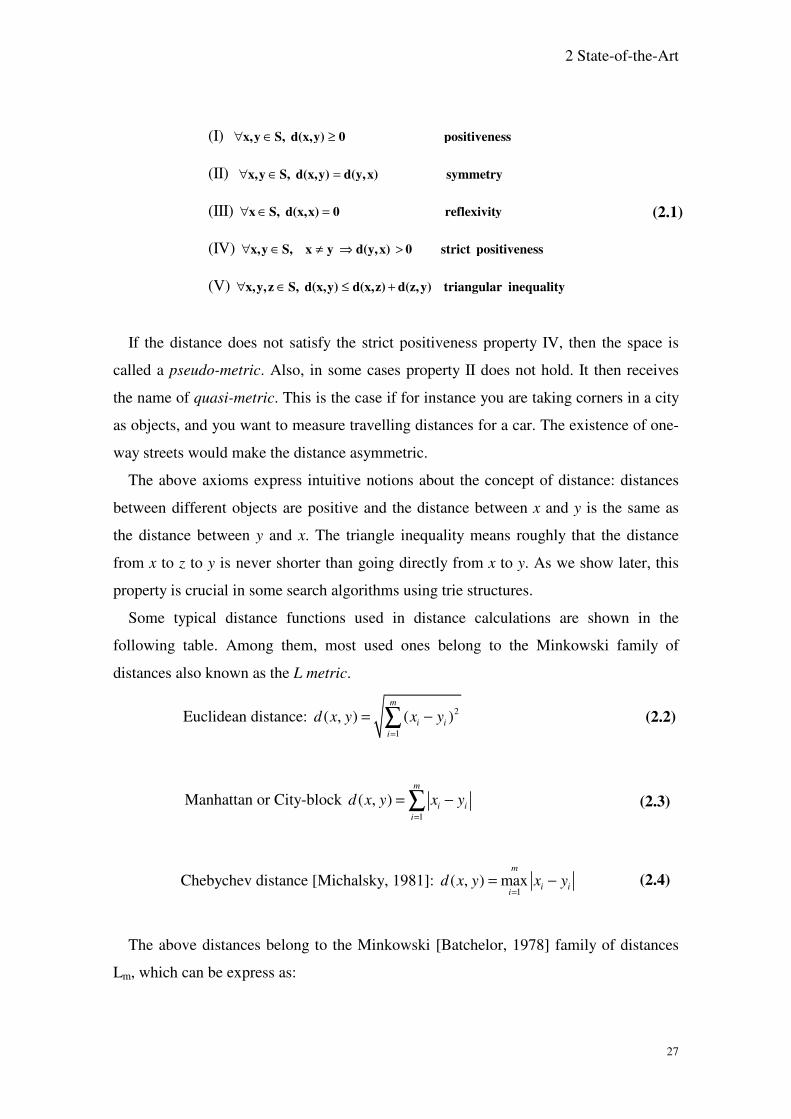
2 State-of-the-Art
27
If the distance does not satisfy the strict positiveness property IV, then the space is
called a pseudo-metric. Also, in some cases property II does not hold. It then receives
the name of quasi-metric. This is the case if for instance you are taking corners in a city
as objects, and you want to measure travelling distances for a car. The existence of one-
way streets would make the distance asymmetric.
The above axioms express intuitive notions about the concept of distance: distances
between different objects are positive and the distance between x and y is the same as
the distance between y and x. The triangle inequality means roughly that the distance
from x to z to y is never shorter than going directly from x to y. As we show later, this
property is crucial in some search algorithms using trie structures.
Some typical distance functions used in distance calculations are shown in the
following table. Among them, most used ones belong to the Minkowski family of
distances also known as the L metric.
Euclidean distance: 2
1
( , ) ( )m
i ii
d x y x y=
= −∑ (2.2)
Manhattan or City-block 1
( , )m
i ii
d x y x y=
= −∑ (2.3)
Chebychev distance [Michalsky, 1981]: 1
( , ) maxm
i iid x y x y
== − (2.4)
The above distances belong to the Minkowski [Batchelor, 1978] family of distances
Lm, which can be express as:
(I) sspositivene 0y)d(x, S,yx, ≥∈∀
(II) symmetry x)d(y,y)d(x, S,yx, =∈∀
(III) yreflexivit 0x)d(x, S,x =∈∀
(IV) sspositivenestrict 0 x)d(y, yx S,yx, >⇒≠∈∀
(V) inequality triangular y)d(z, z)d(x,y)d(x, S,zy,x, +≤∈∀
(2.1)

2 State-of-the-Art
28
1
1
( , )m r
ri i
i
d x y x y=
= − ∑ (2.5)
Other distances are,
Canberra distance: [Michalsky, 1981]
1
( , )m
i i
i i i
x yd x y
x y=
−=+∑ (2.6)
Quadratic distance [Michalsky, 1981]:
( ) ( ) ( ) ( )1 1
( , )T
m m
i i ji j jj i
d x y x y Q x y x y q x y= =
= − − = − −
∑ ∑ (2.7)
Where Q is a problem-specific positive definite m x n weight matrix.
Mahalanobis distance [Nadler, 1993]:
[ ] ( ) ( )1/ 1( , ) det Vm Td x y x y V x y−= − − (2.8)
V is the covariance matrix of A1..Am. and Aj is the vector of values for attribute j
occurring in the training set instances 1..n
Correlation distance [Michalsky, 1981] :
( )( )
( ) ( )1
2 2
1 1
( , )
m
i i i ii
m m
i i i ii i
x x y y
x x y yd x y =
= =
− −
− −
∑=
∑ ∑ (2.9)
where ix = iy and is the average value for attribute i occurring in the training set.
Chi-square distance:
sumi is the sum of all values for attribute i occurring in the training set, and sizex is the
sum of all values in the vector x.
Kendall’s Rank Correlation:
2
1
1( , )m
i i
i i x y
x ysum size size
d x y=
−
= ∑ (2.10)
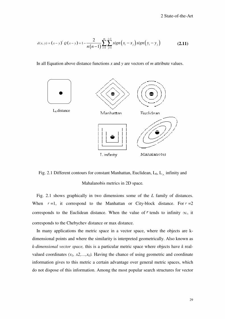
2 State-of-the-Art
29
In all Equation above distance functions x and y are vectors of m attribute values.
Fig. 2.1 Different contours for constant Manhattan, Euclidean, L6, L � infinity and
Mahalanobis metrics in 2D space.
Fig. 2.1 shows graphically in two dimensions some of the L family of distances.
When r =1, it correspond to the Manhattan or City-block distance. For r =2
corresponds to the Euclidean distance. When the value of r tends to infinity d, it
corresponds to the Chebychev distance or max distance.
In many applications the metric space in a vector space, where the objects are k-
dimensional points and where the similarity is interpreted geometrically. Also known as
k-dimensional vector space, this is a particular metric space where objects have k real-
valued coordinates (x1, x2,…,xk). Having the chance of using geometric and coordinate
information gives to this metric a certain advantage over general metric spaces, which
do not dispose of this information. Among the most popular search structures for vector
( ) ( )( ) ( ) ( )
1
1 1
( , ) 12
1T
m i
i j i ji j
d x y x y Q x y sign x x sign y yn n
−
= =
= − − = − − −− ∑∑ (2.11)
L6 distance

2 State-of-the-Art
30
spaces are kd-trees [Bentley, 1975], R-trees [Guttman, 1984], Quad-trees [Samet,
1984], X-trees [Berchtold, 1996] and others.
2.4.3 Types of search
Typically most similarity methods use three types of query within their metric spaces:
1) Range query, where d (q, r) for a query of all elements x within a certain distance r
from q, { }X / ( , ) .u d q u r∈ ≤ A plethora of tree algorithms can be included into this
group, whether they work on discrete or continuous distance functions. A not exhaustive
list includes: BKT (Burhkard-Keller Tree) [Burkhard, 1973], FQT (Fixed-Queries
Tree)[Baeza-Yates, 1994], MT (Metric Tree) [Uhlmann, 1991), SM (Slim Tree)
[Traina, 2000], VPT (Vantage Point Trees) [Yianilos, 1993], BST (Bisector Trees)
[Kalantari, 1983], VT (Voronoi Tree) [Dehne, 1987], M-tree [Ciaccia, 1997]. And still
some of them that can be extended to m-ary trees such as: MVPT (Multi-Vantage-Point
Tree) [Bozkaya, 1997] and GNAT (Geometric Near-neighbour Access Tree) [Brin,
1995].
2) Nearest Neighbour query, or NN. Here to goal is to retrieve the closest elements to
query q in %, which is;
{ }X / X, ( , ) ( , ) .u v d q u d q v∈ ∀ ∈ ≤
3) k-Nearest Neighbour query (k-NN). Similar to the query in (b), but referred to the
k closest objects to q in %. This is, retrieve a set B ⊆ % such that |B| = k and
, , ( , ) ( , ).u B v S B d q u d q v∀ ∈ ∈ − ≤
The last two groups are called in general NN queries or k-NN queries (case (b) been
assimilated when k equals 1). Most of the existing solutions for NN queries uses range-
searching techniques and can be found in most of the tree structures listed under that
query type above.
In all the above types of queries the number of distance evaluations performed gives
the algorithm complexity. At one extreme, all these queries can evaluate all distances
for all objects. In many cases this is impossible to achieve in a reasonable span of time.

2 State-of-the-Art
31
For this reason, most of the time search algorithms pre process an index structure for
data storage, with the goal of saving distance computations when answering similarity
queries. Sometimes there is a high cost in building this structure although this is
balanced with less distance calculations at query time and hence, lower algorithmic
complexity. Some results for IBk, the Weka implementation of an instance-based
learner are presented in Section 7 as a comparison with our own classifier.
2.4.4 Equivalence relations
Search algorithms using an index structure partition the set % into subsets providing a
mapping between data and their classes. At query time some of these are selected to
determine the location of relevant elements; those elements are inspected to provide the
required answer.
In most algorithms this partitioning of the data space generates equivalence relations
between objects in a partition, where partitions, given a set , are denoted as partition
ϕ( ) = {ϕ1, ϕ2…}. This relation, denoted by ~, is a subset of the cross product x ,
the set of ordered pairs of . Two objects x, y � are said to be related, denoted by x ~
y, if they belong to the same partition. This relation is equivalent if it satisfies for all x,
y � the properties of reflexivity (x~x), symmetry (x~y ⇔ y~x) and transitivity (x~y ∧
y~z ⇒ x~z). Every partition ϕ( ) induces an equivalence relation and conversely, every
equivalence relation induces a partition. Hence, an element ϕi of a partition is called an
equivalent class. According with [Chavez, 2001]:
All existing indexing algorithms for proximity searching consist in building an
equivalence relation, so that at search time some classes are discarded and the others
are exhaustively searched. (p.27)
A large class of algorithms to build the equivalence relations are based on pivoting,
which consist in defining a number of representative objects or “pivots” and doing
distance calculation between any object and a given pivot. These receive different
names in the literature: points [Arya, 1998], vantage points [Yianilos, 1993], key
[Bergman, 1999]. The equivalence relation is defined in terms of distance calculations

2 State-of-the-Art
32
between the objects and the pivots: two elements are equivalent if their distance to all
pivots is the same.
Instead of using “pivots”, another large class of algorithms use a different type of
equivalence relation based on “groups”, meaning the proximity to a set of elements.
This algorithms use the Voronoi equivalence relation based on groups {g1, g2,…,gm} is:
x~(gi) y ⇔ closest (x, {gi} = closest (y, {gi})
where closest (x, S) = {w ∈ S, ∀w’ ∈ S, d (z, w) ≤ d (z, w’)} .
The associated partition is the Voronoi partition [Aurenhammer, 1991]. In other
words, in these class of algorithms, the space is divided with one partition for each
group gi and the class of ci is that of the points that have ci as their closest centre.
2.5 Searching in tries
Most trie structures use for searching one of the two mechanisms described in the
previous subsection, namely pivoting or Voronoi “centers”. Next, we give the general
context for searching in tries and talk about some of these algorithms in no particular
order.
Tries are perhaps most widely used in text processing applications, such as string
matching, approximation string matching and compression schemes [Andersson et al.,
1994], as well as in algorithms with genetic sequences, data structures of dynamic
hashing tables, remote sensing imagery, etc [Aoe et al., 1996; Bergman, 1994; Alber et
al., 2001]
Often, when searching in databases, people are often interested in close but not
necessarily exact matches. The problem consist in finding “approximate” matches, such
as spell checking, fingerprint analysis, voice recognition, image understanding and
DNA sequences. These processes use some distance measure to compare how close or
far are objects among themselves. For this reason they are in general computationally
expensive. Therefore, the need for sub linear search is mandatory, hopefully using a
mechanism where most of the database is never directly examined.
Close objects in tries can be searched using a distance metric satisfying the
mathematical equivalent of the triangle inequality, first introduced by [Burckhard et al.,
1973] avoiding complex comparisons to each object in the database. Suppose that given

2 State-of-the-Art
33
objects x, y, z from a dataset R, an integer k, and some distance metric d, it is required to
find all objects in the database with a distance from x of not more than k. The triangle
inequality states that:
�x, y, z ° R, d(x, y) � | d(x, z) - d(y, z)| (2.12)
If we assume now a node p at level l in the trie with value D, every object at leaves
descendant from p has a distance d from the key object keyl. Thus, if |D – d(x, keyl)| > k,
then we know from the triangle inequality above that d(x, s’) is greater than k for all
objects s’ which are descendants of p. Thus search node can be pruned at p.
Taken advantage of this property several search algorithms using tries defined some
set of key objects or central objects from the universal set, being representative for some
data clusters in the data space. Then, as the case for instance of the Triangulation Trie in
[Berman, 1994], the trie becomes a representation of the distances from the objects in
the database to this set of keys. In some remote sensing image problems the
straightforward application of the triangle inequality theorem allows the search
algorithm to discard a substantial number of images to compare in the feature space
[Alber et al., 2001].
In [Berman, 1994] a Triangulation Trie is defined using only a distance measure as a
tool. The only requirement being that this satisfies the triangle inequality property, in
order for the algorithm compares distances only for a selected object’s subset. The
construction of the trie is done first choosing a set of keys from the universal set, that
can be chosen according to some arbitrary convenient criteria. This is important because
the performance of searches in the trie depends on the choice of these keys. For each
object in the database is created a vector consisting of the ordered set of distances to the
key objects. These vectors are input into the trie. Hence, the trie is a compact
representation of the distances from the objects in the database to this set of “keys”.
In [Heinz, 2002], a Burst trie is proposed for searching string text, in which strings
are maintained in order for faster access. Because tries and ternary search trees
[Bentley, 1997], [Clement, 2001] are fast but space-intensive, the proposed structure
compress data into so-called containers linked to a regular trie called access trie.
Searching involves using the first few characters of a query string to identify a particular
container. A list structure or a binary search tree can be used to give form to containers,

2 State-of-the-Art
34
so search within its boundaries is fast. When the container becomes inefficient, it is
burst, that is, replaced by a trie node and a set of child containers holding each one half
of the previously contained strings.
The concept of containers is similar to the previous idea of super nodes developed in
[Berchtold, 1996] on the structure called the X-tree. Observing the problem with the R*-
tree [Beckmann, 1990] consisting in the overlap of the bounding boxes in the directory,
which increases with higher dimensions, the authors proposed a split algorithm
minimizing overlap by the use of super nodes for high dimensional spaces. Overlap is
the percentage of the volume of data that is covered by more than one directory hyper
rectangle. This is correlated to the query performance since in processing queries,
overlap of directory nodes results in the necessity to follow multiple paths, thus
increasing search time.
More formally, the overlap of an R-tree node containing hyper rectangles
{R1,R2,…,Rn} is defined as:
( ).
, {1.. },
, {1.. }
i j
i
R R
i j n i joverlap
Ri j n
∩∪∈ ≠
=∪
∈
(2.13)
||A|| denotes the volume covered by A.
The X-tree consists of three different types of nodes: data nodes, normal directory
nodes and super nodes. Super nodes are large directory nodes of variable size (such as
multiple of the usual block size). The basic goal of these super nodes is to avoid splits in
the directory that result in an inefficient structure.
The LC-trie or level-compressed trie is introduced in [Andersson, 1993, 1994]
corresponding to a compact version of the standard trie data structure. The central idea
in this structure is that the highest complete levels of a trie can be replaced-without
losing any relevant information- by a single node of degree mi, the replacement being
made top-down. If it is assumed that the input consists of independent random strings
from a Bernoulli-type process [Flajolet, 1983], the expected search cost in an LC-trie is
O(log log n), which is significantly better than O(log n), achieved by the conventional
trie.

2 State-of-the-Art
35
2.6 Data Mining and Statistical Sampling
Inductive learning supposes the prior existence of a dataset with records of known
class. Depending on the size of the target population the study of a sample from this
population is sometimes required. Sampling is the subject of this sub-section.
Let us begin by agreeing with [Smyth, 1999] on his assertion that the appreciation of
the fundamental role of statistics in data analysis and in general about statistical ideas is
an aspect often overlook by computer scientists simply by their lack of understanding.
This is due in part by the fact that most courses in computer science give little room for
anything other than a cursory introduction to statistics. This does not mean that our
approach belongs to the stream of statistical data mining, neither that we share the view
of some statisticians that might argue that data mining is not much more than the scaling
up of conventions statistical methods to massive data sets. Indeed Data Mining has
introduced its own ideas for data analysis, which are quite novel and distinct from any
prior work on statistics.
2.6.1 Random sampling
Simply stated, in statistical terms a random sample is a set of items that have been
drawn from a population in such a way that each time an item was selected, every item
in the population had an equal opportunity to appear in the sample This implies that (1)
measurements taken on different items (or trials) are unrelated to one another and (2)
the joint distribution of all variables remains the same for all items [Johnson, 1998].
Choosing a sample, and more specifically a statistical sample as define above is
crucial for instance-based methods. This is particularly true today, in the presence of
huge terabyte databases representing the size of available data we are planning to work
with. It would take long hours if not days to execute the training phase without selecting
just a small subset for this purpose. For this reason sampling is a good solution. But the
results of the algorithm obtained from a sample must be representative for the whole
population. With this in mind the goal consist in selecting a sample from the population,
such that the performance of the mining algorithm is probably close to what it would be
if we run it on the entire database [John, 1996]. At the very least, the selected records to
form the sample should fulfil the requirements of a statistical simple random sample
2 State-of-the-Art
36
(SRS): “A SRS of size n is taken when every possible subset of n units in the populatio n
has the same chance of being the sample” [Lohr, 1999]. This sample set sometimes
called “evaluation” set (often confused in the literature with the “test” set), is used in the
generation of the model function and permits also carrying out the evaluation of the
mining algorithm.
The final goal of evaluation is to measure the accuracy of the algorithm, which is the
probability of correct classification of previously unseen randomly selected records.
These records, only used for this purpose throughout the entire mining process are
known as the test set, and they do not form part of the working sample. Sample records
form the evaluation set, generally called the training set, which is mined to “ learn”
about data patterns, thus allowing the development of the classification algorithm. To
preserve the validity of the estimation, these two sets must be mutually exclusive during
the whole classification process.
Out of the many possible existing bias in selecting sample records, we had two main
concerns in creating the sample. First, the sample should have the characteristics of a
SRS. Second, we want a sample that incorporates class distribution knowledge existing
in the whole population database. The reason for this is obviously related to the final
goal of building a class predictive model.
When not available, information on class distribution can be collected from the
evaluation set, calculating simple probabilities for each class. In some other cases prior
knowledge from the expert domain exists, as is the case with several of available
datasets from the UCI data repository [Murphy, 1994].
It is desirable that the final accuracy of a classifier be estimated using a method with
low variance and bias. For this reason, several accuracy estimation methods exist:
Holdout or Sub-sampling, k-fold Cross-validation, Leave-one-out, Stratification,
Bootstrap [Kohavi, 1995], [Efron et al., 1993], [Mitchell, 1997].
2.6.1.1 Holdout method
The holdout method sometimes called test sample estimation, divide data into two
mutually exclusive subsets called a training set and a test set, or holdout set. It is
common to designate 2/3 of the data as the training set and the remaining 1/3 as the test

2 State-of-the-Art
37
set. The training set is used in the “learning” process while the test set serves t o measure
the quality of the induced classifier.
Formally, let 0 = , q$ be the space of labelled records and R = {r1, r2,...,rn} a
dataset, where ri = <vi � ,i, ci � $>. An inducer I maps a given dataset R into a
classifier � and this in turn maps an unknown record v � , to a class label c � $. The
accuracy of classifier � is the probability of correctly classifying a randomly selected
record:
Acc = P (�(r) = c) for a randomly selected instance <r, c> � 0.
Further let Rh be the holdout set, which is a subset of R of size h, and let *t = R / Rh.
The holdout estimated accuracy is defined as:
( )( , )
1( , , ),
i i h
h t i iv c R
Acc C R v ch
ϕ∈
= ∑ (2.14)
where K(i, j)=1 if i = 0, and 0 otherwise [Kohavi, 1995].
2.6.1.2 Cross-validation method
Cross validation is a method aiming to estimate the error of a given hypothesis
generated by a concept-learning algorithm (classifier). The method specifically refers to
generalization error, which is the error on data that has not been seen during training.
The method is called sometimes k-fold-cross-validation or rotation estimation to
indicate that the inducer is trained and tested k times.
Given a set of training data and a concept learner this is how cross validation
estimates the accuracy of the hypothesis gained by running the learning algorithm on
the data set:
Randomly divide the training data in k mutually exclusive sub-sets, called the “ folds”
R1, R2, R3, Rk of approximately equal size. For each one of the k folds t = {1,2,k} the
classifier is trained using R/ Rt and tested on Rt. The resulting cross-validation accuracy
estimation is the average of the k times the classifier is tested.
Formally, let R (i) be the test set that include record ri = <vi, c>. Also let I(R, v) be the
label assigned to an unlabelled instance v by the classifier build by inducer I on dataset
R. Then the accuracy of a cross-validation estimate is given by:

2 State-of-the-Art
38
( )( )( , )
1( / , , ).
i i
h i i iv c R
Acc I R R v ch
ϕ∈
= ∑ (2.15)
2.6.1.3 Leave one out method
A special case of cross validation is the so-called leave one out method, where k is
chosen as the cardinality of the training set. In other words, for each given example
another run of learning is performed using all training data except for this example and
the correctness of the classification of the single example left out is checked.
For efficiency reasons leave one out is unusual in practice, although in general it will
be closest to the real error. Instead, k=10 is a frequently chosen compromise between
computational effort and quality of estimation results.
2.6.1.4 Bootstrap method
Bootstrap was introduced by [Efron et al., 1993], and consists in given an evaluation
file of size n, to create a so-called bootstrap sample by sampling n records uniformly
from data with replacement. This is the training set. All other records form the test set.
Since the sample is obtained with replacement, the probability of not being part of this
list is (1 – 1/n)n � e-1 � 0.368, and the expected number of distinct objects from the
original dataset appearing in the test set is 0.632n. For instance, consider a dataset R =
{1,2,3,4,5,6,7,8,9,10,11,12}. Randomly sampling n instances with replacement would
produce the following training set D = {1,2,10,7,10,5,6,10,5,1}. The remaining
instances would form the test set T = {3,4,8,9}.

- 39 -
3 The Trie-Class Algorithm. Basic definitions
In this Section we provide a general overview of the Trie-Class algorithm and most of
the basic definitions and functions used throughout this thesis, including some
examples. We also explain in detail the search mechanism used to extract nearest
neighbours and compare its classification skills with a regular k-NN algorithm.
3.1 General overview of the algorithm
Our approach to induction is partially based on the instance-based methodology or
Nearest Neighbours (NN) [Cover, 1967; Salzberg, 1990; Aha, 1991], sometimes also
known as case-based reasoning (CBR) [Aha, 1998]. In general, the basic notions of NN
and instance-based methods are the storage of learning data, the use of some metric to
carry out similarity computations by means of calculating distances, and some indexing
scheme to help the searching mechanism. A distinctive characteristic of NN and CBR in
particular is its “ lazy” approach to problem solving. According to [Aha, 1998] pure lazy
problem solvers exhibit three typical behaviours:
• They defer processing the input until they receive a query request. They just
store input examples.
• They are data-driven, meaning that they respond to requests by combining
information from the stored data and,
• They discard any temporary intermediate results created during problem
solving.
NN methods also present a more eager approach, resembling to a certain extent some
model-based approaches in that they retain their inputs into an intensional6 data
structure, reply to queries using this structure and keep it for future requests.
Combining elements that characterize these methods along with ideas from Decision
Trees our approach uses a tree structure as an index to store cells from training data in
order to “learn” , permitting at the same time a very fast search of “ similar” instances.
In a second thinking phase, queries on unseen instances are answered using training
instances as model. Two of these instances will be selected from the data structure,
6 Including the rules that describe the inner structure of objects

3 The Trie-Class Algorithm. Basic definitions
40
using a non-Euclidean distance on an attribute-by-attribute basis without normalization.
Later, we use different criteria to select one of them as the best available pattern
representation of the new unseen instance, as will be explained in Section 6.
3.2 Basic definitions
Notation {r R, c L | exp1(r,c) exp2(r,c)}∈ ∈ • stand for the set of values of exp2
when r and c take values in R and L, and exp1 is true. If exp2(r,c) = r then the
expression is reduced to {r ∈ R | exp1(r)}.
Definition 1. Let’s consider the closed universe formed by a data file R composed of
a finite set of N records r.
R = {r1, r2,..,rN } . (3.1)
In Supervised Machine Learning we find data containing a set of instances, each one
described by a vector of attributes and a class label. Attributes are considered to be
predictor or relevant attributes. They are used as independent variables to induce a
certain classification hypothesis, which in turn is used to predict the class of an instance,
considered the dependent variable. Therefore, much of this thesis is referred to attributes
(or features as they are also called), its characteristics, types and values, and the way
they can be used to generate the description of the concept, which is at the centre of the
learning process.
Definition 2. In any given record r we find a finite set of Ai attributes belonging to set
S,
1 2 i nS = {A ,A ,..A ,..,A }, a nonempty set. (3.2)
Definition 3. Each record r is formed by the Cartesian product of n attribute values
A1|a1 x A2|a2 x...x An|an and a class label c. Each attribute Ai has its corresponding value
ai, which belongs to domain Ti, such that:

3 The Trie-Class Algorithm. Basic definitions
41
1 2 = , ,.., , , (1.. ), , .n i ir a a a c i n a T c L∈ ∈ ∈ (3.3)
Definition 4. Every record r is associated with one of c class labels belonging to a set
L.7
{ }1 2, ,.., lL c c c .= (3.4)
Definition 5. Each class label c belonging to records r is obtained by the following
function:
label(r) = c if r = <a, c> . (3.5)
3.3 Definitions on cell discretization
In many Data Mining applications large amounts of data as well as large instance
vector dimensions demand some form of data reduction. This is particularly true for
methods based on instances or Nearest Neighbours. One of the aspects of the problem
attacked by Trie-Class, is to reduce the dimension of each feature by reducing the
number of possible values an attribute can take. This goal can be reached by applying
discretization to data domains, particularly interesting in attributes exhibiting continue-
value types. At the same time, discretization is required in order to work with metric
spaces and distance calculations. Discretization has the disadvantage of a potential
information loss, allowing two different attribute values to coexist within a given
interval thus increasing entropy, a measure of the degree of purity of a given interval
with respect to the class. However, the advantage of reducing the search space, a
fundamental problem facing almost all algorithms in Data Mining, many times is not
harmful for real-world applications [Weiss et al., 1998]. In Trie-Class, discretization is
applied to numeric attributes whether discrete or continuous. In the case of nominal
attributes, simply each nominal value is assigned a partition of its own.
7 In this thesis we use indistinctively the words class label, class or just label.

3 The Trie-Class Algorithm. Basic definitions
42
Definition 6. The domain of each attribute Ai can be partitioned into a finite number
of user-defined intervals within domain Ti. The number of these intervals can range
from 1 to si. We assume the existence of function ordi(), which converts the value of an
attribute into its corresponding discrete value vi, which is an ordinal representing the
interval value:
( ), (0.. ), .i i i i i iv ord a v s a Ti= = ∈ (3.6)
We call value vi a cell component, which along with other components form cell p as
shown later in Equation (3.10).
Definition 7. Let Mi and mi, be the maximum and minimum attribute values within
domain Ti, where wi is the size of each interval si. The number of intervals si is simply
the ratio of the number of elements in the attribute domain over wi, a real number.
( ) 1, 0 .i i
i ii
M ms w
w
− + = >
(3.7)
Definition 8. Each numerical attribute value ai fits into an interval represented by the
discrete cell component vi, which is computed using the following floor function:
( ) .i ii i i i
i i
a mv ord a s
M m −= = × −
(3.8)
If ai = mi, then the value of vi will fit into interval zero.
Definition 9. For categorical or symbolic attributes, attribute ai has its corresponding
interval value simply calculated as:
vi = ordi(ai) . (3.9)
If a priori knowledge domain information exists on the actual order of symbolic
attributes, then vi represents the corresponding order number, which in Trie-Class is set

3 The Trie-Class Algorithm. Basic definitions
43
in a dictionary file (described in Section 7). If the interval value calculation for a
symbolic attribute does not represent a problem, the same is not true when we want to
calculate de distance between these types of values. This is the topic of Section 4.2.
Notice that the number of intervals si is not the same for all attributes. They depend
on values Mi and mi, as well as the interval size. These parameters are user-defined. In
our implementation, they are declared in the dictionary file. Although not implemented,
parameter si, could be automatically computed by the system given the simple
mechanism we use for domain partitioning as explain above.
Example 3.1
Imagine that a certain record r exhibit the value for attribute ai = 9. Let’s assume that
the domain for this attribute is formed by discrete values ranging from mi =1 to Mi =10;
with wi = 2. Applying Equation (3.7) we obtain si = 5. Then, applying function ordi()
from Equation (3.8) we would obtain vi = ordi(9) = 4. Every vi value will fit into one of
si intervals belonging to the partition of attribute Ai. In this case, interval number 4
corresponds to the fifth interval, as they begin with interval 0.
If we convert all attribute values from a record into its corresponding interval values
vi we obtain cell p.
Definition 10. All vi elements together form a cell vector p containing n component
element values vi. We call P the set of all cells p obtained from set R.
Example 3.2
Imagine that we have the following record vector containing five attribute/value
pairs: r = <a1=9, a2=3,a3=5 , a4=6, a5=1>.
( )1 2 1 = , ,.., ,.., , , 0.. .i n i ip v v v v p P v s −∀ ∈ ∀ ∈ (3.10)

3 The Trie-Class Algorithm. Basic definitions
44
As in the previous example the values for the following variables are: mi =1, Mi =10,
wi = 2 and si = 5. Applying functions ordi() from Equation (3.8) to each attribute value
ai and arranging according with Equation (3.10) we convert record r into cell p:
p = < v1= 4, v2 = 1, v3 = 2, v4 = 2, v5 =0>
Some specific cells used in this thesis are px, p1, p2, etc. Cell px is a new cell from an
instance of unknown class. Cells p1 and p2 are cells belonging to the training set with
known class.
Definition 11. A multi-attribute-value vector cell p is obtained from its corresponding
instance vector r from Equation (3.3) using function cel(r) such that:
( )( ), (1.. )1 n i i ip = cel(r) with p = <v ,..,v >, v ord a r i n= = (3.11)
Most classification algorithms and in particular k-NN algorithms consider instance
vectors relating to a given label as a whole. In Trie-Class we develop the idea of sub-
cell or prefix (as known in text data), which can be associated with one or more classes.
In this way, it is possible an “earl ier” class membership identification using just a subset
of the entire cell, which allows data compression for concept description, a desired goal
for the attribute selection problem. Sub-cells are define as follows:
Definition 12. In every cell p we find n sub-cells qi, which correspond to its prefix:
1 2, ,.., , (1.. ). So ,i i iq v v v i n p q u= = = (3.12)
where u is the suffix portion. Therefore, we find sub-cells containing 1, 2,..n
component elements, where the last of them, called qn is identical to the full cell p.
The number of records in the dataset exhibiting cell vector p are returned by calling
function freq(p):
{ }( ) # | ( ) .freq p r R cel r p= ∈ = (3.13)
Function freq can be equally applied to any sub-cell qi:

3 The Trie-Class Algorithm. Basic definitions
45
{ }( ) # | ( ) ,i ifreq q r R cel r q u= ∈ = (3.14)
Definition 13. We define function kfreq() as the total number of records where its ith
value falls into interval k.
{ } ( , ) # | v with ( ( )) .i i ir Rkfreq i k k v ord a r∈= = = (3.15)
Hereafter we will just write vi to indicate the full expression vi = ord(ai(r)).
A restricted variation of the previous function includes the additional argument c
meaning that a restriction is imposed to objects in interval k: they must belong to class
c. Next function measures the number of sub-cells in a given interval relating to just one
label.
Definition 14. Function lfreq() produce as result the number of records in a dataset
where its vi cell component is k and its label is c:
{ } ( )( , , ) # | vir R k label r clfreq i k c ∈ = ∧ == (3.16)
Definition 15. We define function labels(p) as the set of labels found in the subset of
records with cell p.
{ }( ) , | ( ) ( ) labels p r R c L cel r p label r c c= ∈ ∈ = ∧ = • (3.17)
Definition 16. The number of class labels attached to a given cell p is given by the
following function:
( )( ) #nlabels p labels p= (3.18)
the same function can be applied to sub-cells:

3 The Trie-Class Algorithm. Basic definitions
46
( )( ) #i inlabels q labels q= (3.19)
In most evaluation sets R there is a predominant class label, meaning that most
records hold that class. In the literature this is known as “ default rule” [Domingos,
1996; Brodley, 1996].We call this “majority class ” as explained in Section 6.
Definition 17. The class frequency of a given class correspond to the number or
records in a dataset associated with that class.
{ }( ) # | ( )cfreq c r R label r c= ∈ = (3.20)
Using the previous function we define function lmaj() as the function that returns the
majority class, which is the predominant class in a set R.
We now turn our attention to a characteristic aspect of sub-cells, namely its degree of
relationship to one or more classes. The intuition here is that we are interested in sub-
cells formed by a minimum number of cell component elements relating to one class
only. This idea comes from a fundamental concept in Information Theory known as the
Minimum Description Length (MDL) principle [Risannen, 1978].
Roughly speaking, the MDL principle states that the “best” theory t o induce from
training data is the one that minimizes the complexity of the theory and the length of the
data encoded with respect to the theory. In terms of the sub-cells defined by Trie-Class,
the shorter the number of attributes in a sub-cell sequence identifying just one class, the
strongest this sub-cell is in terms of concept description. We call this the strength of a
cell and we measure it using the following function.
Definition 18. The strength of a cell corresponds to the size of some sub-cell qi, at the
ith component element where it becomes associated with just one label:
{ }( ) # 1 | ( ) 1istrength p i n nlabels q= ≤ ≤ = (3.21)
Vector cells with greater strength represents vectors located in larger homogeneous
areas of the nth dimensional space. Therefore, a strong cell means that more of its vi
values belong to the subset of values associated with a given class. For this reason we

3 The Trie-Class Algorithm. Basic definitions
47
are interested in strong cells as their predictive capability has more confidence when
compared with others of less strength.
3.4 Exclusiveness as a measure of attribute relevance
Using some of the functions from the previous subsection, we define now some
additional concepts, helping to define the criterion used to determine how relevant a
given attribute is.
Whether the discretization method takes or not into account an instance’s class
membership, all intervals present some class distribution. Our interest is to discover
class distribution information within sub-cells, in order to get the kind of information
that might be hidden due to a non-supervised discretization process like ours. If
intervals belonging to some attribute exhibit a class distribution where one of the
existing classes is predominant in relative terms compared with the others, then we are
in the presence of semi-exclusive attributes, which we define next.
Definition 19. Attribute Ai is said to be semi-exclusive for interval k, if function
semk() is true. Parameter M is a user-defined value representing the fraction of records in
interval k with class c. Function semk() is defined as:
( , , ) (( ( , , ) / ( , )) )semk i k c L lfreq i k c kfreq i kϕ ϕ= ∃ ∈ • ≥ (3.22)
If function semk() is true when M equals 1, then we have an exclusive interval, i.e. all
vi values in interval k belongs to the same class. In the literature these intervals are
known as primary [Turney, 1996], [Kohavi et al., 1997] or pure intervals [Holte, R.,
1993]. The opposite is the concept of maximum impurity, indicating that all classes are
equally represented on each interval of a given partition [Brodley, 1995]. Modifying the
value of M allows function semk() to return true in more or less homogeneous class
regions of the instance space. This would be the case for instance of a dataset with four
classes with one of them say cj representing 60% of the class distribution in a given
interval k. Setting the value of parameter M to 1 in function semk() would provided no
information for the region covering that interval. Setting the value of M = 60 instead,

3 The Trie-Class Algorithm. Basic definitions
48
function semk() would return true allowing to visualize the predominance of class cj,
thus allowing using this information regarding the class at the sub-cell level.
Finding how many of these semi-exclusive intervals exist in whole cells is calculated
using the function from next Definition 20:
Definition 20. The degree of exclusiveness of a cell p corresponds to the fraction i of its
n cell component values falling into intervals conforming to the semi-exclusive property.
This property is calculated with the following function:
( ){ }( , ) # 1.. | semk( , , ) /isemp p i n i v i nϕ ϕ= ∈ • (3.23)
We are interested in the fraction of intervals belonging to a given cell complying with
the semi-exclusive property when this refers to the same class, so we can have consistent
information. Used this way, the presence of one or more intervals of this type increases
the probability for the cell to be associated with a given class. Hence, cells having
intervals exhibiting this property constitute important class pattern predictors.
Definition 21. If all discrete vi values belonging to attribute Ai � R are projected into
its corresponding intervals, then the degree of relevance of attribute Ai with value ai
denoted with symbol Gi, correspond to the fraction of records falling into those intervals
where function semk() is true with respect to the total number of records in R.
( )( ){ }i i# | ( , , ) /ir R k ord a r semk i k r Nδ ϕ= ∈ = ∧ • (3.24)
Parameter N represents the total number of records in set R..
Large values for / means a more relevant attribute when compared with others. The
opposite represents irrelevant attributes. The next example illustrates this.
Example 3.3
Let’s calculate the value of parameter / for two attributes, A1 and A2, each having
domain si partitioned in ten equal sized intervals as in Fig. 3.1. The dataset has two
classes: A and B. Frequencies for each interval are shown in the row labelled “ freq”.

3 The Trie-Class Algorithm. Basic definitions
49
Notice that in this case it does not matter which is the predominant class in the set of
semi-exclusive intervals included in the calculation of parameter /�as it is the case with
function semp(). This is so because it is perfectly possible for the same attribute to have
different values that can be associated with different classes. This is precisely what
matters for attribute relevance. How many values determine cell class membership.
Projecting attribute A1 values into intervals vi , with � = 0.75
vi 0 1 2 3 4 5 6 7 8 9 Total � freq 77 32 62 49 79 20 12 23 11 43 408 Class * * * * * * * * A A 54
54/408=0.132
Projecting attribute A2 values into intervals vi , with � = 0.75
vi 0 1 2 3 4 5 6 7 8 9 Total � freq 227 23 35 17 17 14 12 13 5 45 408 class * A * * B B * B * B 112
112/408=0.274
Note: An asterisk means intervals where function semk() is false. Shadow areas represent intervals
where semk() is true with � = 0.75.
Fig. 3.1 Attribute values projection in one-dimension to depict its relevance
3.5 Attribute selection
Trie-Class uses a tree structure to hold cell patterns as a mean of speeding up
searching most similar objects. As search begins in the root of the tree, the input order
of attributes is fundamental if we want most similar instances to remain close to each
other in the data hyperspace. For this reason determining the order of attributes is a pre-
processing phase executed before tree insertion. (Tree build is explained in Section 7).
Definition 22. The predictive skill of attributes is a measure of its degree of
relevance as defined in Equation (3.24). According with this relevance attributes can be
ranked in decreasing order of relevance.
1 2 1, ,.., ,.., , | | | (1.. ).i n i i i nβ δ δ δ δ δ δ += ⟨ ⟩ ≥ ∈ (3.25)
Attributes where its relevance /i = 0, are orderly pushed to the list’s end. These are
candidates for elimination (“pruning”), which can be done to improve algorithm

3 The Trie-Class Algorithm. Basic definitions
50
complexity at the expense of some loss in accuracy as shown in Section 4.. An example
of a dataset features ordered by its degree of relevance is shown next in Example 3.4.
Example 3.4
Let’s consider the Cancer -Wisconsin dataset from Section (5.1.3). It contains nine
working numeric attributes representing patient data for cancer diagnosis. Applying
formula from Equation (3.24) for each attribute in this dataset, we obtain the following
/�values shown in Table 3.1 below. They are ranked by its degree of relevance.
Table 3.1 Attributes degree of relevance values in Cancer dataset
Nº Attribute name Frequency Gi 1 Uniformity of Cell Size 89 0.218 2 Uniformity of Cell Shape 69 0.169 3 Marginal Adhesion 59 0.145 4 Normal Nucleoli 58 0.142 5 Clump Thickness 54 0.132 6 Bland Chromatin 34 0.083 7 Mitosis 22 0.054 8 Single Epithelial Cell Size 16 0.039 9 Bare Nuclei 9 0.022
We show results later in Section 4 showing how classification accuracy changes with
changes in accuracy using only relevant attributes.
3.6 Shape definitions
The similarity hypothesis sustains that what defines a class is that its members are
similar to each other and not similar to member of other classes. Therefore, object
similarity is determined using distance calculation between corresponding attribute
values using functions such as Euclidean or Manhattan.
We are now interested in exploring additional information that might be useful to
describe the similarity concept. One such case is constituted by the information
concerning intra-attribute relationships within a cell. One of these is the relationship
between consecutive attributes belonging to the same cell, which can be represented
using the slope representation between these two points.

3 The Trie-Class Algorithm. Basic definitions
51
Fig. 3.2 Slope intersection form of a line
For a given line in the xy-plane making angle R with the x-axis, the slope m is a constant
given by tan ,y
mx
θ∆≡ =∆
where �x and �y are changes in the two coordinates over some
distance. In general, a slope represents a quantity, which gives the inclination of a curve
or line with respect to another curve or line such as the one in Fig. 3.2.
We could graphically represent the shape form of a given n-dimensional cell p
drawing in two-dimensions all segment lines between pairs of consecutive attributes.
We do this by converting each a cell component element into a point. We use the actual
attribute value as the y-coordinate and we assign the attribute’s order numb er as the x-
coordinate. Hence, we could draw all segment lines between the discrete points (1,v1),
(2,v2),..,(n,vn). As we keep constant �x each segment, segment �y = (yi – yi-1)
corresponds to a slope between consecutive cell values. An example of such shape
representation can be seen in Figure 3.3. In total we would have n-1 line segments to
represent a given shape.
Designing a shape retrieval method involves other than shape representation, the
definition of some similarity measure and the way these shapes will be accessed or
retrieved. [Mehrotra, et al., 1995]. To answer this we first define the space H as the
space of all h shapes. Within this space shape similarities are found using some distance
x
b
y
�
y = mx + b

3 The Trie-Class Algorithm. Basic definitions
52
d(h1,h2) in order to compare two shapes. Within this framework we propose the
following definitions:
Fig. 3.3 A two-dimensional representation of a cell
Definition 23. The shape of a cell is defined as the sequence of its m slope
components between consecutive values:
1 2 1 1 1, ,.., ,.., , m ( ), , with ,..,i n i i i nh m m m m v v h H p v v− +=< > = − ∈ =< > (3.26)
This newly created shape vector contains positive and negative slope values and is
one dimension shorter than the cell vector from which is built. The new space H
represents a space change with respect to space Rn. As can be easily seen this space is
not metric as some of its properties are not satisfied, namely, positiveness and
symmetry. Within this space we can use a distance measure to determine how close or
similar two shapes are from each other. We do that using the following function.
Definition 24. The shape similarity between two cells, corresponds to the distance
between its corresponding shapes:
' '( , ) ( , )sp p p d h h= (3.27)
Distance d(h’, h ) can be any of the standard distances belonging to the Minkowski
family explained earlier in Section 2.4.2.
(5,v5)
(1,v1)
y
x
shape of p
(2,v2) (4,v4)
(3,v3)
(6,v6)

3 The Trie-Class Algorithm. Basic definitions
53
Using shape distances to represent cell similarities can help identifying shape
patterns in a shape data space. If similar shapes relate to the same class, then this
information can enrich the similarity concept.
The degree of shape similarity between two shapes is affected by the actual value of
each slope and the slope sign itself, which indicates the relationship between two
consecutive attribute values. We illustrate in example 3.5 shape construction and a
similarity function.
Example 3.5
Imagine a dataset containing five cells p1,p2,..,p5, belonging to some training set, each
one formed by seven cell components. Cell values are indicated in Table 3.2.
Table 3.2 Cell vectors and their component values
Cell component values Cells v1 v2 v3 v4 v5 v6 v7
p1 3 6 4 9 4 1 9 p2 17 10 14 9 9 11 6 p3 1 19 13 23 10 2 3 p4 12 9 7 4 8 15 19 p5 15 5 13 8 7 13 4 px 19 9 15 8 9 12 5
The task consists in classifying a new cell px from the test set using the shape
similarity function. Let’s first convert all cell vectors from Table 3.2 into shape vectors
applying the shape formula in (3.26). We obtain the shapes and its values indicated in
Table 3.3.
Table 3.3 Shape vectors corresponding to cells from Table 3.2
1( )i iv v+ − h1 3 -2 5 -5 -3 8
h2 -7 4 -5 0 2 -5 h3 18 -6 10 -13 -8 1 h4 -3 -2 -3 4 7 4 h5 -10 8 -5 -1 6 -9 hx -10 6 -7 1 3 -7
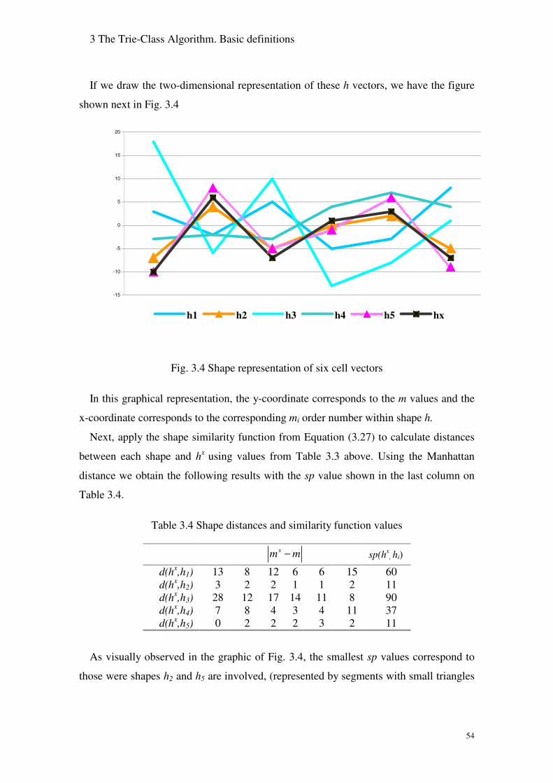
3 The Trie-Class Algorithm. Basic definitions
54
If we draw the two-dimensional representation of these h vectors, we have the figure
shown next in Fig. 3.4
-15
-10
-5
0
5
10
15
20
order position values
h1 h2 h3 h4 h5 hx
Fig. 3.4 Shape representation of six cell vectors
In this graphical representation, the y-coordinate corresponds to the m values and the
x-coordinate corresponds to the corresponding mi order number within shape h.
Next, apply the shape similarity function from Equation (3.27) to calculate distances
between each shape and hx using values from Table 3.3 above. Using the Manhattan
distance we obtain the following results with the sp value shown in the last column on
Table 3.4.
Table 3.4 Shape distances and similarity function values
xm m− sp(hx, hi)
d(hx,h1) 13 8 12 6 6 15 60 d(hx,h2) 3 2 2 1 1 2 11 d(hx,h3) 28 12 17 14 11 8 90 d(hx,h4) 7 8 4 3 4 11 37 d(hx,h5) 0 2 2 2 3 2 11
As visually observed in the graphic of Fig. 3.4, the smallest sp values correspond to
those were shapes h2 and h5 are involved, (represented by segments with small triangles
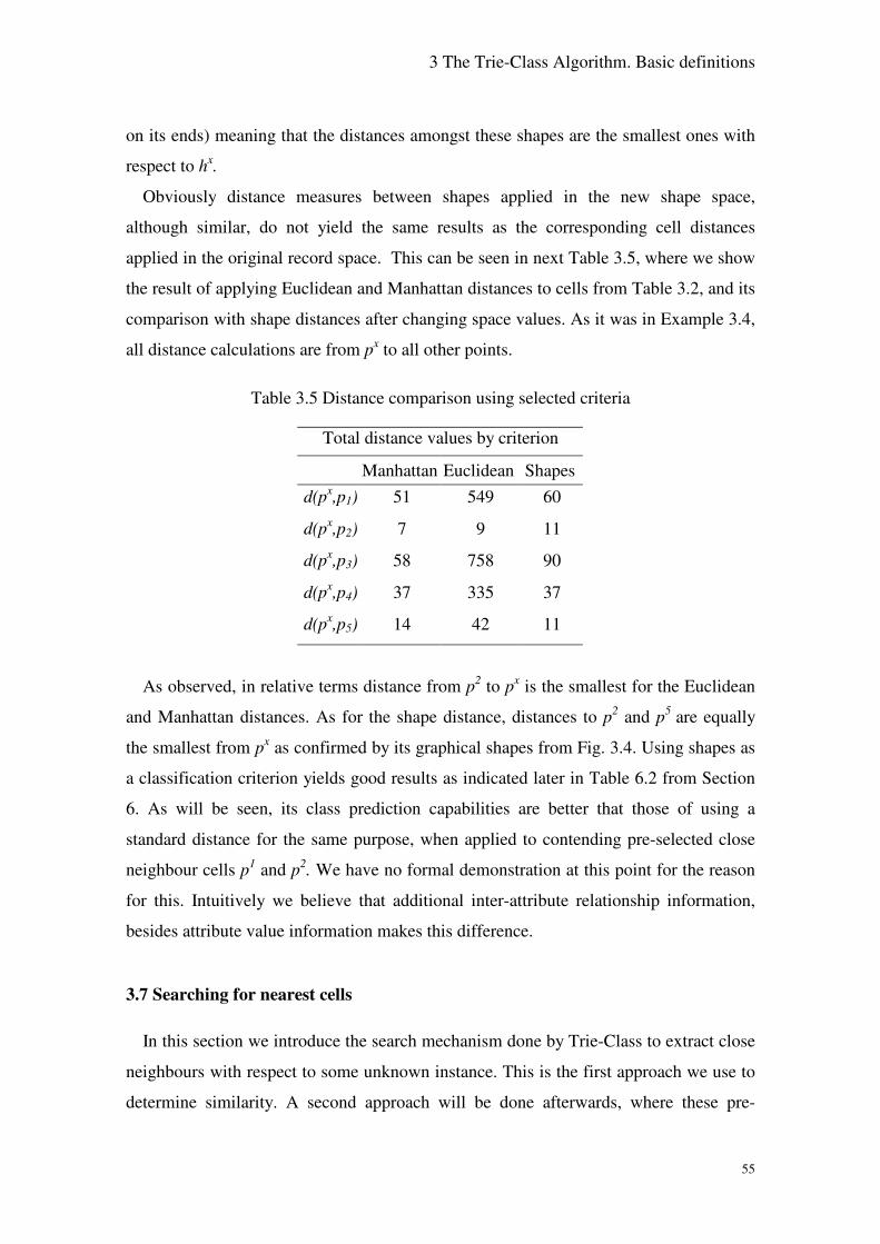
3 The Trie-Class Algorithm. Basic definitions
55
on its ends) meaning that the distances amongst these shapes are the smallest ones with
respect to hx.
Obviously distance measures between shapes applied in the new shape space,
although similar, do not yield the same results as the corresponding cell distances
applied in the original record space. This can be seen in next Table 3.5, where we show
the result of applying Euclidean and Manhattan distances to cells from Table 3.2, and its
comparison with shape distances after changing space values. As it was in Example 3.4,
all distance calculations are from px to all other points.
Table 3.5 Distance comparison using selected criteria
Total distance values by criterion
Manhattan Euclidean Shapes d(px,p1) 51 549 60
d(px,p2) 7 9 11
d(px,p3) 58 758 90
d(px,p4) 37 335 37
d(px,p5) 14 42 11
As observed, in relative terms distance from p2 to px is the smallest for the Euclidean
and Manhattan distances. As for the shape distance, distances to p2 and p5 are equally
the smallest from px as confirmed by its graphical shapes from Fig. 3.4. Using shapes as
a classification criterion yields good results as indicated later in Table 6.2 from Section
6. As will be seen, its class prediction capabilities are better that those of using a
standard distance for the same purpose, when applied to contending pre-selected close
neighbour cells p1 and p2. We have no formal demonstration at this point for the reason
for this. Intuitively we believe that additional inter-attribute relationship information,
besides attribute value information makes this difference.
3.7 Searching for nearest cells
In this section we introduce the search mechanism done by Trie-Class to extract close
neighbours with respect to some unknown instance. This is the first approach we use to
determine similarity. A second approach will be done afterwards, where these pre-

3 The Trie-Class Algorithm. Basic definitions
56
selected cell patterns are carefully inspected through the use of Decision Parameters
explained in Section 6.
Eventually, the number of close neighbours selected could be any. We have chosen to
implement our algorithm for just two of them, and we have kept this number in view of
our results.
The method we propose here to find nearest neighbours does not use the standard
family of distances used by regular k-NN methods. It corresponds to a “greedy” search
method in general, as the best solution at each point is taken using only available
information at each node of the tree structure. To illustrate this, lets assume the
existence of a new query cell px with format as in Equation (3.10). Lets call p+ the ideal
closest object to px in the entire dataset. The algorithm’s task consists in extracting the
closest cell to p+ and as a result the algorithm will obtain a cell we call p1
In the original NN algorithm this is done using a “brute force” method or some type
of index, applying to them the Euclidean distance from px to considered objects. In our
case distance calculation proceeds attribute by attribute, restricting the allowable search
space for a given attribute based on previous attribute values. The allowable search
space keeps cell component values in order, so the closest elements to pxi are searched
starting at pxi-1 and px
i+1 respectively. The search proceeds to both “sides” of pxi looking
for the closest element. As soon as one of these values is closer to pxi it is selected. Trie-
Class uses a tree structure, which exactly allows doing this.
If we call cells p1 and p2 the two “closest” objects to px found in a space with those
characteristics, then it will be always true that:
1 2( , ) ( , ) and ( , ) ( , )x x x xd p p d p p d p p d p p+ +≤ ≤
We argue later in Section 7 that objects p1 and p2 are more rapidly extracted using this
structure when compared with regular NN methods, and also that they are better class
predictors. In the next subsections we explain the way this is done introducing a general
search algorithm for a closest cell, which is the same independently of the number of
cell patterns that might be extracted.

3 The Trie-Class Algorithm. Basic definitions
57
3.7.1 Selecting closest pattern
The algorithm extracts close cells one by one. In our case it first get cell p1. To do this
initially dispose of the entire set P as its search data space. The extraction of cell p1
progress adding one more cell component at a time, where these cell components are the
ones found closer to its corresponding px elements. As the search progresses, smaller
and smaller subsets of P constitute the allowable search space to obtain the next cell
component element. For each one of these Pi spaces its dimension and location is given
by the values forming the corresponding sub-cell qi. We explain next the way this space
is defined.
The extraction of any cell is done attribute by attribute, with the algorithm proceeding
incrementally. Any sub-cell qi is of the form qi = �qi-1, k! where k is the next cell
component element. Starting with i = 1, assuming an empty sub-cell q0= <�> and
knowing element qi-1, the problem consist in finding some interval k1 representing the
next cell component, which is the closest value to the unknown element kx. The found
element k1 must satisfy the following property:
( ) ( ) ( )1 11
x xik K q k k k k−∀ ∈ • − ≤ − (3.28)
Where the set K(qi) is defined by:
( ) { },i iiK q k | q k P= < >∈ (3.29)
Cell component k1 is the closest element to kx among the elements in K(q) and Pi
correspond to its search space. As each new cell component element ki is added, the
search space for next element k1+1 is further restricted to the space defined by the
previous sub-cell qi which is Pi. So the search space of the last element gets confined to
space Pn, thus avoiding the search of most of the total data space.
Notice that as it happens with decision trees, the selection of each new k element
divides the space into axis-parallel hyper planes.
From the class viewpoint, as long as the search process does not reach the last cell
component member, or sub-cell qi is not associated with just one class, the selection of

3 The Trie-Class Algorithm. Basic definitions
58
the next k element does not impose a class restriction. What matters is to find each time
the closest cell component element to the corresponding query element.
What happens if two k values are equidistant from kx?
In this case frequencies are used as the first option to break this tie. Including
frequency as part of the search criterion mechanism aims to avoid outliers8. It also helps
avoiding overfitting, defined as the case of a hypothesis that fits the training data and
exists another hypothesis that fits less well the same data which performs better over the
entire distribution of instances [Mitchell, 1997].
Therefore, the algorithm chooses the k value where freq(q1) is maximum including
the new potential element k. A larger frequency in this context is interpreted as an
indication of a close distance, as done in some k-NN algorithms [Dasarathy, 1991].
After cell p1 has been selected the algorithm proceeds searching for cell p2. The
search mechanism is the same as the one already described, except that this time set
K(q) has an additional restriction: all objects considered must belong to a class which
must be different from the one in p1.
Originally, cell p1 with class say c1 was extracted from some set R. As the class
associated with p1 cannot be in any other subsequent cell extracted p2, p3,.., pn, we
remove from the original set R all cells having class c1. We call R1 this new subset,
which correspond to the complimentary search space where cell p2 will be extracted. No
cells with the class of the already extracted p1 form part of this space. Follows that if
subsequent cells were extracted after extracting p2, the restricted space would become
R2, R3,..,Rm, reducing each time the allowable search space, where Rm is the data space
corresponding to the search space for cell pattern pm+1.
This entire operation is equivalent to have training records belonging to the same
class inserted in different trees and executing sequentially the search on each tree.
The following definition represent the above described search process.
Definition 25.
We define function neighbours() as the function that returns two cells p1 and p2
representing the closest neighbours found with respect to some unknown cell px using
the search process already described.

3 The Trie-Class Algorithm. Basic definitions
59
(p1, p2) = neighbours(px) (3.30)
It is worth noticing the fact that restricting search spaces starting from the first
attribute is equivalent to give more eliminatory power to more relevant attributes.
Search spaces allowed for less relevant attributes are restricted. As a greedy search
selects the best path based solely on tree node information, more precise solutions could
be lost. And in this sense, relevant attributes do not have more weight in this process but
just the power to eliminate some options.
3.7.2 Using look-ahead to solve ties in cell pattern selection
It is known that greedy search produces sub-optimal solutions [Goodman et al.,
1988]. In view of cheap available computing power, is worth trying to improve these
solutions without much extra algorithmic complexity. For this reason, if frequencies in
candidate cell component elements are also equal, the algorithm applies a “look ahead ”
mechanism. This consists in looking for next closest element ki+1 on each conflicting
sub-cell with ki as the next potential component. The process is repeated until is found
some component is closer to the respective kxj component, or until the end of the cell is
reached. When such element is found along this path, the algorithm chose it as the new
component element, along with all k values in the path all the way up to the conflicting
parent component ki.
Using this type of limited look-ahead search although it produces an increase on
algorithmic complexity, it is controlled by the fact that it is only applied as a last
resource to solve tie situations. However, in datasets with larger intervals where chances
of equal sub-cells increase, execution times will increase. In general, our results show
that limited look-ahead as the one used here produced acceptable execution times.
As a last resort, if ties persist and the last cell component has been reached, the
algorithm chooses arbitrarily one of the conflicting k values as the new component. At
the end of this process, any selected full cell close to px is associated with just one class.
Trie-Class never fails to find an identical full cell to px, if such cell exists in the
training file as the search process for the next bigger and smaller values with respect to
8 See subsection 3.9.1

3 The Trie-Class Algorithm. Basic definitions
60
px for each attribute begins with this value. In this special case, if cell p1 equals px, the
search algorithm stops looking for other close cells. It simply assigns the class of the
identical pattern found to px. This also means that running against training records, Trie-
Class classifies without errors.
3.7.3 The search algorithm in practice
Example 3.6
Lets assume the existence of a dataset with the following five cell patterns:
Table 3.6 Original search space P containing 5 cells and a new query
cell v1 v2 v3 v4 v5 v6 v7 class p2 3 1 1 1 3 2 1 A p1 3 1 1 2 1 1 3 A p4 3 1 1 2 5 6 9 B p5 3 5 3 4 1 2 1 A p3 8 5 4 7 9 6 3 B px 4 3 2 5 3 1 5 ?
The last row contains the unknown cell px. In order to search for the closest cell to px,
the algorithm proceeds as follows:
________________________________________________________________
Set q1 = <�> Search for the closest value to px
1 = 4. The algorithm finds values 3 and 8. Value 3 is selected after comparison. Incorporate value, so q1 = <3>. Next, look for next elements closest to px
2 = 3. Elements 1 and 5 are found, which are equidistant. So we use the frequency criterion. Sub-cell <3,1> has larger frequency than sub-cell <3,5>. Therefore, insert new cell component giving q1 = <3,1> Repeat the process looking for closer element to target px
3 =2 among v3 values. The only available option is again 1. After insertion we have q1 = <3,1,1>. The closest elements to qx
4 = 5 is 2 so q1 = <3,1,1,2>. At this stage there are two possible candidate elements: p1
5 =1 and p45 = 5. Both are
equidistant from qx5 = 3 (a distance of 2 units). Which one to chose?
As frequency is equal in both conflicting sub-cells apply look ahead technique. Then look into each of corresponding 6th elements, p1
6 = 1 and p46 = 6.
Calculate distances between them and chose the closest one. As d(px6, p1
6) = 0 then this element is chosen and also its parent. So now q1 = <3,1,1,2,1,1>.
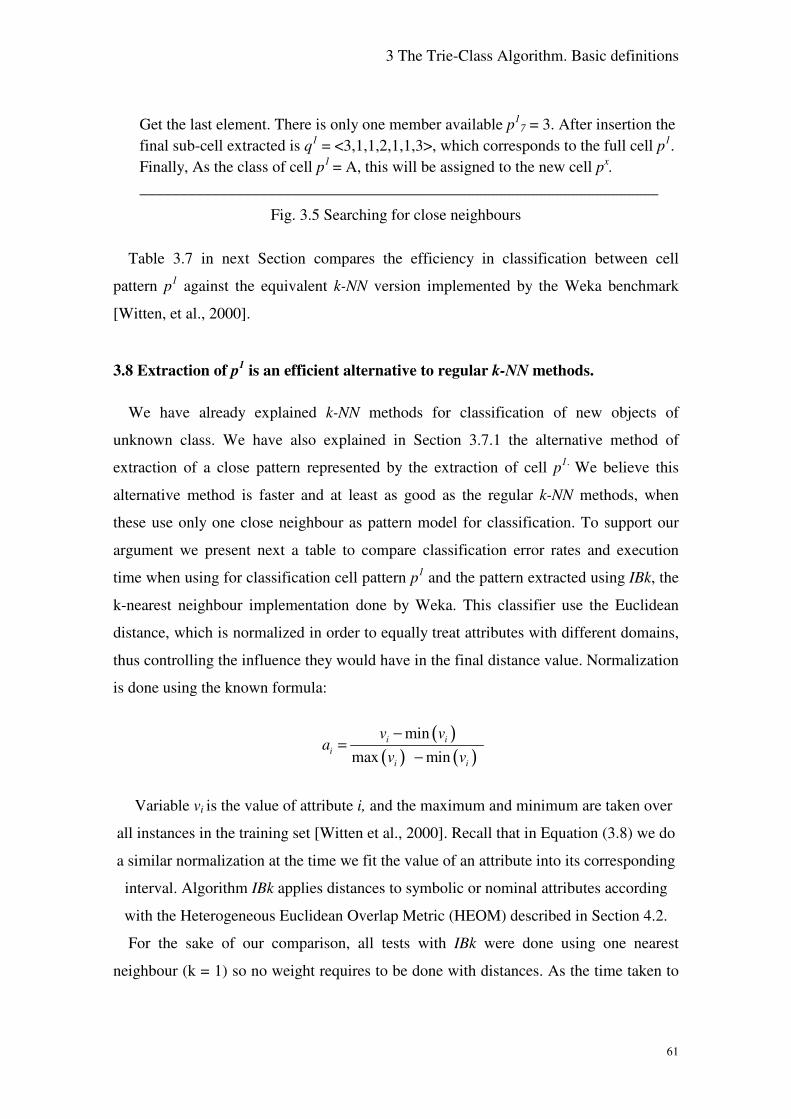
3 The Trie-Class Algorithm. Basic definitions
61
Get the last element. There is only one member available p17 = 3. After insertion the
final sub-cell extracted is q1 = <3,1,1,2,1,1,3>, which corresponds to the full cell p1. Finally, As the class of cell p1 = A, this will be assigned to the new cell px. _________________________________________________________________
Fig. 3.5 Searching for close neighbours
Table 3.7 in next Section compares the efficiency in classification between cell
pattern p1 against the equivalent k-NN version implemented by the Weka benchmark
[Witten, et al., 2000].
3.8 Extraction of p1 is an efficient alternative to regular k-NN methods.
We have already explained k-NN methods for classification of new objects of
unknown class. We have also explained in Section 3.7.1 the alternative method of
extraction of a close pattern represented by the extraction of cell p1. We believe this
alternative method is faster and at least as good as the regular k-NN methods, when
these use only one close neighbour as pattern model for classification. To support our
argument we present next a table to compare classification error rates and execution
time when using for classification cell pattern p1 and the pattern extracted using IBk, the
k-nearest neighbour implementation done by Weka. This classifier use the Euclidean
distance, which is normalized in order to equally treat attributes with different domains,
thus controlling the influence they would have in the final distance value. Normalization
is done using the known formula:
( )( ) ( )
minmax min
i ii
i i
v va
v v
−=
−
Variable vi is the value of attribute i, and the maximum and minimum are taken over
all instances in the training set [Witten et al., 2000]. Recall that in Equation (3.8) we do
a similar normalization at the time we fit the value of an attribute into its corresponding
interval. Algorithm IBk applies distances to symbolic or nominal attributes according
with the Heterogeneous Euclidean Overlap Metric (HEOM) described in Section 4.2.
For the sake of our comparison, all tests with IBk were done using one nearest
neighbour (k = 1) so no weight requires to be done with distances. As the time taken to

3 The Trie-Class Algorithm. Basic definitions
62
classify a test instance increases linearly with the number of training instances that are
kept in the classifier, sometimes is required to restrict this number, which in Weka is
done by setting up a window size option.
In our case this option has not been used. Instead, and for both algorithms we do a
dataset split of 60% of records for training and 40% for test.
Table 3.7 Classification error rates comparing p1 and IBk algorithm
Dataset % Error Difference Time (s)9 Difference
Nº recs.test Name p1
Trie-Class IBk
Weka % p1
Trie-Class IBk seconds
1 17637 Adult 18.3 21.2 2.9 309 4080 3771 2 360 Annealing 2.3 1.4 -0.9 45 4 -41 3 280 Breast-cancer-W 5.5 4.6 -0.9 1 1 0 4 144 Dermatology 7.5 6.3 -1.2 2 1 -1 5 308 Pima Diabetes 24.0 29.5 5.5 2 1 -1 6 21556 Forest cover 24.9 11.7 -13.2 2400 6600 4200 7 122 Heart disease Cl. 30 22.1 -7.9 1 1 0 8 108 Heart Statlog 22.4 27.8 5.4 1 1 0 9 1509 Hypothyroid 1.0 9.7 8.74 30 60 30 10 60 Iris 2.4 5.0 2.6 1 1 0 11 4397 Pendigits 2.3 0.8 -1.5 120 348 228 12 1774 Satimage 12.0 18.4 6.4 25 33 8 13 400 German credit 27.4 27.5 0.1 3 3 0 Average gain of p1 in error rates and execution time 6.0 8194
All execution times are expressed in seconds10. In the case of IBk figures comes from
the tool itself. As can be seen in Table 3.7, on thirteen datasets Trie-Class is on average
6% better and it took over two hours less time to execute than IBk. Error figures for IBk
are less good if we compared with those obtained doing 10-fold cross-validation from
Table 5.15. As the execution time goes up, Trie-Class executes better than IBk. Initially
Trie-Class is better in 7 out of 13 cases, which represents 54% of cases. When execution
time goes over 15 seconds, Trie-Class is better in 71% of cases and this percentage
further increases to 75% for the case of datasets where the running time took more than
25 seconds. In other words, as complexity goes up, Trie-Class almost constant search
procedure shows its value. In datasets Adult, Forest cover and Pendigits, execution time
9 Wall clock time measured as running time in a standard PC with a single process running.

3 The Trie-Class Algorithm. Basic definitions
63
took over 2 minutes. In all of them IBk takes at least 3 times more execution time than
Trie-Class.
Trie-Class classification error increases using only p1 as the sole criterion for
classification when compared with figures using the full algorithm, as will be show in
Table 5.15 on Section 5.
3.9 General assumptions on some basic Principles
In this thesis, we adopt assumptions on data, which follow some general accepted
principles. We enumerate and briefly explain each one of them.
3.9.1 Data consistency
A basic assumption in this thesis is that the overwhelming majority of instances in N
are consistent, i.e. each unique cell vector gets associated with only one class, which is a
standard assumption as found in [Everitt, 1981;Titterington, 1985; Cios, 1998; Quinlan,
1996].
All training cells where nlabels(p) > 1 represent two or more cells with identical cell
component values, but with different class. Therefore these cell patterns provide no
information class-wise. The cause for this might be that at least one of these cells
constitute noise, which corresponds to instances for which either the class label is
incorrect, some number of the attribute values are incorrect or a combination of the two
[Brodley, 1995]. In some other cases noise data can correspond to a type of data called
outliers, data items lying very far from the main body of the data [Kaski, 1997].
In any case, conflicting cells still are located within the same area in the nth-
dimensional data space. This brings us back to the basic assumption of the nearest
neighbour paradigm: instances that are close to each other will have similar posterior
class probabilities [Dasarathy, 1991]. For this reason, in these cases Trie-Class eliminate
from the search the identical conflicting cells looking for the next close cell pattern in
the same area.
10 Trie-Class is implemented in C, not in Java as Weka, So part of time differences can be attached to this factor.

3 The Trie-Class Algorithm. Basic definitions
64
3.9.2 Partition granularity
As we will explain in Section 4, Trie-Class pre-process data before tree building, in
such a way that independently of the data type of attributes, their values are discretized.
Discretization is the process by which the domain of a continuous attribute is partitioned
into a finite number of intervals. This discretization is done using Equations (3.7), (3.8)
and (3.9).
In general, small numeric attributes domain, whether discrete or continuous are not
discretized at all and the corresponding unit of the domain is used as a default partition,
as in Trie-Class this is more a data structure requirement rather than a step in the
classification process itself.
In any case, for any cell p � P we assume that the granularity of all partitions
generated by the discretization process is such, that allows every cell in the training set
to have a known label, making function nlabels(p) = 1.
3.9.3 Class membership, Patterns and the Continuity Principle
Which is the spatial class distribution of object in Supervised Learning?
Are similar classes distributed into continuous areas in that space or rather they are
scattered throughout that space at random?
Intuitively, one might think that class distribution in real data tend to be
characterized by continuity, meaning that there exists some correlation between
attribute values and its mapping to classes, and therefore there are data areas of
continuous class distribution. Many classification algorithms compress the feature space
based on the certainty that just a few attributes bear the key to class membership. If this
is the case, then class distribution indeed presents spatial continuity.
We apply this principle to rather small regions of the dimensional R space covered by
cells of the same class. If a new cell of unknown class falls into one of these regions,
and existing training cells of the same class are located at distances representing upper
and lower boundary values with respect to the unknown object, then we assume that its
class is the same as the one hold by cells in that neighbour area.
In Trie-Class specifically we apply this principle to sub-cells q as defined in Equation
(3.12).

3 The Trie-Class Algorithm. Basic definitions
65
For instance, lets suppose the existence of sub-cells: <qi-1, k1> ° P and <qi-1, k2> ° P
Applying function labels from Equation (3.17) to sub-cells we obtain:
labels(<qi-1, k1>) = {c} and labels(<qi-1, k2>) = {c} then, for a new interval k °
[k1,k2] labels(<qi-1, k>) = {c}
Thus, in interval k sub-cells will also exhibit class c. This criterion is applied in Trie-
Class for all spatial areas with no available pattern information provided that cells with
the same class bound those regions. In that sense, every other possible new query cell px
is always approximated to some of the existing classes in the dataset.


- 67 -
4 Pre-processing Data Before Mining
The task of extracting knowledge cannot even begin without preparing data to fulfil
the requirements of a particular mining algorithm.
Preparation time taken before mining data represents a considerable portion of the
whole knowledge extraction process. This fact is often overlooked by researchers
fighting for a split second of execution time, forgetting the hours if not days spent in the
preparation of data. For a given algorithm, the number of tasks involved in pre-
processing data is independent of the size of the database. In any case, the farther apart
the data format is with respect to the needs of the algorithm, the longer the time it takes
to complete pre-processing it.
Preparation time must not only be considered as the manipulation of data itself, but as
their overall comprehension and meaning. Before anything else we have to know about
data characteristics and its representation, including type of variables and their meaning,
the type of noise and missing data which we might expect, information about the classes
and its distribution, the frequency of updates and the cost of misclassification among
others. But most important of all, we definitely have to know the purpose of the data
owner, and the exact notion of the problem he/she wants to solve. This is fundamental,
if we are planning to make any sense out of data.
In the rest of this section, we explain the data preparation needed prior to tree
construction and execution including sample selection, attribute value discretization, the
treatment of categorical attributes, attribute selection and the effects of changing
interval size after discretization.
4.1 Converting records into discretized patterns
Attribute values belong to one of several data types: qualitative or non-numerical
(symbolic, linguistic), quantitative or numerical (continuous, discrete). Because our
classification algorithm and the ranking of attributes are based in a nominal space, all
continuous attributes are first discretized. This is done, based on the information taken
from a user-supplied dictionary file11.
11 For a layout of the dictionary, see Annex I.

4 Pre-processing Data Before Mining
68
Discretization is the process of partitioning the domain of a continuous attribute into a
finite number of intervals [Lebowitz, 1985].
There are three criteria to classify discretization methods: global vs. local, supervised
vs. unsupervised, and static vs. dynamic [Dougherty, 1995]. Numerous discretization
methods used to induce one-level decision trees and instance-based methods utilize the
class label in the partitioning of the data space [Payne, 1998]. Others use domain
specific information [Lebowitz, 1985; Aha, 1995]. Still in some other cases the
discretization process consider the number of instances in the interval [Cattlet, 1991].
We use the Equal Interval Width (EIW) single feature discretization method (sometimes
called binning) [Wong et al., 1987], which do not make use of instance classes in the
discretization process. For this reason sometimes it is called unsupervised discretization
method.
Intervals are represented by discrete integers using the symbol si, which corresponds
to the number of intervals within a given domain. Function ord() described in (3.8) does
this conversion. Notice that when ai and mi are equal, vi equals zero, which corresponds
to the first possible interval value. The number of intervals obtained on each partition,
are given by Equation in (3.7). For attributes represented by rational numbers the
corresponding interval value is calculated according to Equation (3.8). For categorical
attributes this simply corresponds to its ordinal value, as described in Equation (3.9).
If a priori knowledge on domain information exists on the actual order of symbolic
attributes, as done in some discretization methods [Kerber, 1992], then the interval
value represents the corresponding order number, which is set in the dictionary (see
Appendix I). Next section specifically deals with symbolic attributes. If this information
does not exist, one has to be careful of not imposing any order on these values. In
[Brodley, 1995a], when a feature has more than two observed values, then each feature-
value pair can be mapped to a prepositional feature, which becomes true if and only if
the feature has the particular value in the instance. We explain in Section 4.2 the
distance between two unordered symbolic values done in Trie-Class.
It could be argued that using binning as discretization method causes us to lose
information about the class distribution in the nth dimensional space. This effect is even
more negative, in methods where discretization is done with the purpose of identifying
class membership, using the so-called impurity or goodness measures. [Murthy et al.,
4 Pre-processing Data Before Mining
69
1994]. The goal of most of these methods is to use discretization as an important
component of the classification model. Some examples of these methods are Gini Index
criterion [Breiman et al., 1984], Minimum Description Length [Rissanen, 1978],
information gain [Quinlan, 1986], ChiMerge system [Kerber, 1992], recursive entropy
discretization [Fayyad et al., 1993], Max minority [Heath et al., 1993], maximal
marginal entropy [Chmielewski et al, 1994], StatDisc [Richeldi et al., 1995].
Although inferior to the entropy family of methods as shown in [Fayyad et al., 1993],
the difference in performance between equal width discretization and some of these
methods is small [Dougherty et al., 1995].
Other than the simplicity and lower computational cost of this method our goal with
discretization has to do with storing training records in an index of manageable size, in
order to increase searching efficiency, as long as the number of partitions is
representative of the concept description. Partitioning attribute domains into si intervals
helps reducing tree size as well as in some cases allowing concept generalization. The
well-known loss of information problem derived from discretization is attenuated in our
case. The most important information for each sub-cell individually considered is its
class. With this respect, the only negative effect of this is class overlapping, which has
the net effect of postponing class membership in sub-cells as they increase their size of
component members.
As additional help to attenuate some loss of information due to discretization, we
keep class distribution information for semi exclusive values in a specific file as
explained later on Section 7.
It has also being related the equal width binning mechanism to a higher sensibility to
outliers [Dougherty, 1995]. To help with this, semi-exclusive intervals can be tuned
setting parameter M in Equation (3.22) to a somewhat larger threshold value.
4.2 The special case of categorical attributes
Many Machine Learning and Pattern Recognition methods require that input take the
form of numeric values. As Trie-Class uses a distance calculation for the extraction of
near neighbours to some unknown cell px, the presence of symbolic attribute types
represent a problem of its own. Symbolic values are values representing concepts that
cannot be ordered, and therefore, there is not an obvious distance between them. This is

4 Pre-processing Data Before Mining
70
the case for instance for the letters of the alphabet, or concepts such as “ red”, “white ”
and “blue” (provided we do not consider their wave length values of course). Near
neighbours methods resort to special metric schemes to solve the similarity problem in
these cases, a problem central to pattern matching.
Many methods have been proposed in the literature to overcome this problem, such as
the Value Difference Metric (VDM) from [Stanfill, 1986], counting the features that
match as in [Towel, 1990], the PEBLS system that incorporate MVDM, a modified
version of VDM in [Cost, 1993]; the basic idea of the later being that two values of the
same attribute are similar if they give similar likelihood for all possible classifications.
Also, the Heterogeneous Euclidean Overlap Metric (HEOM) which basically attributes
binary values to distances depending whether two values of the same attribute are equal
or not equal, the Minimum Risk Metric (MRM) which directly minimizes the risk of
misclassification using conditional probabilities [Blanzieri, 1999].
In many cases applications symbolic attributes appear along with continuous
attributes. For this reason it is used a heterogeneous distance function, as is the case
with the software IB1, IB2 and IB3 [Aha et al., 1991; 1992] as well as the one used in
[Giraud-Carrier et al., 1995]. This function defines the distance between two values x
and y of a given attribute a as:
( )( )
1,,
,
if x or y is unknown, else
d x y overlap(x,y) if a is nominal, elsearn_diff x ya
=
(4.1)
When any of the attributes is unknown a maximal distance of 1 is returned.
The overlap function is defined as:
( ) 0,,
1, if x = y
overlap x yotherwise
=
(4.2)
and the range-normalized difference rn_diff is defined as:

4 Pre-processing Data Before Mining
71
( )_ ,mina
a a
x yrn diff x y
max
−=
− (4.3)
Where maxa and mina are the maximum and minimum values respectively observed in
the training set for attribute a. The normalization serves to scale the attribute down to
the point where differences are most of the time less than one.
Overall, Trie-Class uses a heterogeneous distance calculation. The first one explained
in Section 3.7 search cell patterns close to the unknown cell px. The second one used
within the context of decision parameters, use a straightforward distance calculation
when comparing two already pre-selected cell patterns, which will be shown in Section
6.1.2.
For the case of symbolic attributes, Trie-Class uses a simple distance calculation. It is
based on conditional probabilities in order to determine the distance between categorical
attributes. As it was explained in Section 3.7, for the ith attribute belonging to the
unknown sub-cell qx = <qxi-1, qx
i>, the problem consist in determining whether element
qxi is closer to element k1 or element k2 both belonging to the set of sub-cells p = <qi-1,
k>.
If qx presents the same value of some existing element k, then distance is zero and
element k is selected. If not, Trie-Class uses the distance computation that we explain
next.
Definition 26. The distance between two categorical attributes vx and vi given the
class c of vi, depends on the probability of class c given value vx.
( ) ( )0, ,
( , )1 | | , , , ,
x i
x ix i x i
i i i
if v v elsed v v
P c v label v c c c L v v s
== − = ∈ ∈ (4.4)
Expression P(c | v) expresses the conditional probability of class c given value vx and
it is calculated as the prior probability of c times the joint probability of c and v:
( ) ( ) ( ),P c v P c P c v= ∩< (4.5)
The meaning of this distance calculation is simple: the larger the probability that vx is
associated to the class of vi, the shorter the distance between them. When this

4 Pre-processing Data Before Mining
72
probability is zero, the distance is a maximum, i.e., equal to one. If the probability is the
maximum then distance is zero.
As can be seen, this distance depends on the Prior Probability of a given class,
represented as P(c), and the joint probability of value vx and the class associated with
value vi.
When comparing distances d(qx, k1|c1) and d(qx, k2|c2) where c1 and c2 represent the
known classes of k1 and k2, the distance calculation is indirectly calculated and restricted
only to the correlation of qx against classes c1 and c2.
The intuition behind this is simple. When choosing the next closest element for sub-
pattern qx, the only reference is the class associated with each of the two contending
members. Therefore, the “closest” neighbour will be the one where its class correspond
to the class that qx also better relates.
When the label associated with vi is unknown and labels(qi) > 1, Trie-Class resort to
one of the options of the general search case, which were described in Section 3.7. In all
other cases the algorithm uses Equation (4.1). This mechanism works better than the
simple overlap idea of Equation (4.4).
We tested for this effect datasets Adult, Annealing, German credit and Census, which
contain an important number of symbolic attributes. Classification performance when
considering distance as decision parameter did improve on average over 2.5% when
compared with the simple overlap distance for the same datasets.
Next we show a simple example of distance calculation for symbolic attributes as
done by Trie-Class.
Example 4.1
Suppose a dataset formed by multidimensional attribute vectors, and attribute Ai is
symbolic and its domain set consisting of Ai = {v1= “ blue”, v 2 = “red”, v 3 = “yellow” }.
The set of available classes in this dataset is L = {c1 = “A”, c2 = “B”, c3 = “C”}. Table
4.1 below shows prior class probabilities hypotheses and also joint probabilities for each
class given the value. These data was compiled using training set data.
Imagine we are given a new query value for sub-cell qx = (v3 = yellow, c = ?) with
unknown class. Using the search process Trie-Class comes up with two possibilities as

4 Pre-processing Data Before Mining
73
the nearest sub-cells: q1 = (v1 = blue, c1), and q2 = (v2 = red, c2). The problem consist to
know whether value yellow is closer to value blue or red, i.e., whether distance d1(v3,v1)
is greater or smaller than distance d2(v3,v2).
Table 4.1 Class distributions by value for a symbolic attribute
Categorical values Class hypotheses
c1 c2 c3 Prior class hypotheses P(c) 0.50 0.30 0.20 1.0 v1=blue 0.40 0.30 0.25 v2=red P(c�v) 0.24 0.04 0.45 v3=yellow 0.36 0.66 0.30 Class probability 1.00 1.00 1.00
Using values from Table 4.1 and applying Equation (4.1) we obtain the following
results:
d1(v3, v1) = (1 – 0.18) = 0.820 and d2(v3 ,v2) = (1 – 0.198) = 0.802.
So d1(v3, v1) > d2(v3, v2), value yellow is closer to value red than to value blue. Thus,
there is a greater likelihood that the class corresponding to value yellow is c2, which is
the class associated with value red.
4.3 Feature reduction and elimination
Data Mining techniques face the challenge represented by the so-called
dimensionality problem. Often, data is represented by datasets containing N instances
each of them formed by n features or attributes. Sometimes know as multivariate data, it
can be thought of as a (N x n) data matrix. The dimensionality n plays a significant role
in multivariate modelling. In text classification problems, web traffic, commercial
supermarket transactions or clustering of gene expression data, n can be as large as 103
or 104 dimensions and the amount of data needed according to density estimation theory
scales exponentially in n. This is the so-called “ curse of dimensionality” problem.
Fortunately, transaction data is typically sparse, meaning that only a small percentage of
the entries in the N x n matrix are nonzero. Taking advantage of this, the idea of using
subsets of items or itemsets has been developed in market basket analysis, which

4 Pre-processing Data Before Mining
74
represent “ information nuggets” in large high -dimensional transaction datasets. Finding
frequent itemsets from a sparse set of transaction data is one solution for the problem as
studied by [Agrawal, 1993] and more recently in [Han, 2001].
Not only the number of attributes poses a formidable complexity problem but also the
fact that, not all attributes contribute equally to solve classification problems.
Within this context, two well-known problems arise when using decision tree
structures and instance-based algorithms for supervised learning, which are of interest to
us. Firstly, the attribute’s input order heavily determines the predicting skills of the
algorithm. The reason for this is that some attributes have more discrimination power
than others predicting the right class for the unknown instance. Choosing the wrong
order of attributes could move values apart in the hyperspace that otherwise would be
closer. For instance imagine than in a tree, the fifth attribute is the one with a larger
statistical correlation with a given class in the dataset under analysis. Two records with
identical values for attribute five, but having different values in the previous four
attributes would end quite distantly from each other in the hyperspace, misleading the
classification algorithm. For this reason, at input time when building the tree we want
attributes ordered by their discriminatory power with respect to class labels, as done for
instance in some rule induction algorithms [Quinlan, 1986] [Cover, 1967], [De
Mántaras, 1991].
Secondly, the presence of irrelevant attributes increases computational cost and can
mislead distance metrics calculations [Indyk, 2000]. This is particularly true for nearest
neighbour algorithms, which determine the class label of an unknown instance using the
geometric concept of proximity, which involves the notion of distance between points in
a n-dimensional space [Lee et al., 1984]. As the position of the instance is defined by
the value of its attributes, if these are not relevant, then the basic assumption is violated.
Based on these, attributes are characterized as relevant or irrelevant, in terms of their
degree of contribution to the classification hypothesis [Kohavi, 1997; Lebowitz, 1985]12.
The complexity of feature selection algorithms is related among other factors to the
number and quality of attributes. Searching most relevant attributes cannot be
exhaustive in many cases. The dimension of datasets is exponential in the number of
12 These authors still identify redundant attributes, a situation which we do not address here.

4 Pre-processing Data Before Mining
75
attributes. Hence, verifying every other possible combination of best attributes is, in
many cases, out of the question [Lesh, 1998].
In this section we present a low computational and simple empirical algorithm for the
supervised learning task in order to:
• Establish a criterion to decide which attributes are relevant.
• Choose the best attribute input order for processing.
• To diminish classification algorithm complexity, as well as increasing or at
least preserving its predictive skills.
4.3.1 Ordering attributes
In general, our method ranks attributes by its capacity of predicting classes as in
[Gennari et al., 1989]. We measure this capability without directly taking directly into
consideration other attributes from the original sequence. Indirectly, inter-attribute
relationship exists; attribute values are not independent from the value of other
attributes in a given pattern, as is the case in most real life cell vectors.
We postulate that this capacity of influencing class prediction increases, when a given
attribute interval shows a significant frequency of values fully or predominantly
associated with one class as defined in Equation (3.22). In this sense, we soften the
Boolean definition found in [Kohavi et al., 1997].
How and how much significant the frequency of these type of patterns in a given
interval should be, and the way it could be used as a measure for attribute relevance is
the topic of the next sub-section.
4.3.2 Looking at sub-cells from the “clearest” viewpoint
Our objective is to find the most useful discriminative attributes with the purpose of
improving the classifier prediction accuracy [Guyon, 2001]. This heuristic criterion has
been used successfully before [Liu et al., 2000].
We have already stated in Section 3 that strong sub-cells with small values for i
(shorter sub-cells) where nlabels(qi) = 1, represent large areas of the data space related
to one class. If a new instance to be classified falls into one of these areas, its chances of
correct classification increase. Most of its neighbours will share the same label. For this

4 Pre-processing Data Before Mining
76
reason, we are interested in looking at the entire data space from the viewpoint of
attributes with larger number of examples where classes are “visible ” directly from
them. Using this simple criterion would avoid endless combination of possibilities as
done in traditional attribute selection methods [Miller, 1990; Brodley et al., 1995;
Kohavi et al., 1997] among others.
In any dataset R, visibility relates to the problem of looking at the data space from the
viewpoint that allows a better view to existing classes. Take for instance the well-known
example of looking at four numbered tennis balls suspended in a three-dimensional
space as shown in Fig. 4.1. Suppose that the objective of the viewer is to be able to
distinguish the tennis ball numbers. Looking at that space from different angles
represented by the three bulb lights in Fig. 4.1, more or less ball numbers are
distinguish. All solutions lie in the hyperspace. Our problem consists in finding them13.
We consider being more relevant attributes allowing a better view of larger number of
sub-cells in terms of class membership. On Fig. 4.1, the view from “A” is the only one
that allows full visibility of the 4 ball numbers. This is the most interesting view if the
goal was to discover as much ball numbers as we could.
The shortest sub-cell contains only one component element is q1 = <p1, c>. If it does
relate to one class only, it means that larger areas of the hyperspace relate also to one
class label. And by the principle of continuity the probability of correctly classifying
new instances falling into these intervals also increase.
3
21
3 4
2
4
3
1
4
2
41
2
13
Fig. 4.1 Different views on the same set of solutions
C
A
A
B
BB

4 Pre-processing Data Before Mining
77
To identify better views on the data space from the viewpoint of an attribute all of its
values are projected into a one-dimensional discretized space, as was shown in Fig. 3.1.
This corresponds to build the root node of a multi-way tree using one attribute. This
resembles the 1R classification system [Holte, 1993] although in this system the ranking
of features is based directly on error rates using each individual attribute as the sole
classification hypothesis. In our case we are interested in the total number of sub-cells
components found in semi-exclusive intervals define in Equation (3.22), for a given
attribute Ai and M values. Attributes showing more individual cells in semi-exclusive
intervals are also more relevant as calculated by variable G defined in Equation (3.24).
The intuition behind this is that trees formed using these attributes in top levels will
produce larger data areas associated with one class, helping to define early class
membership in the data hyperspace. Based on this, we can set attribute relevance as a
measure allowing attribute comparison as explained in the next section.
To avoid the effect of outliers, in the form of few cells laying in one interval related
to one class, a minimum number of records in one semi-exclusive interval can be set as
a constrain in Equation (3.22). For instance, [Holte, 1993] used 3 and 6 as minimum
existing values on his tests.
4.3.3 Reducing attribute numbers
Ranking attributes is done according with attributes relevance as we already
explained in Section 3.5. As we will show in our results (Section 5), doing this
improves the predictive accuracy of the classification algorithm.
Reducing the number of irrelevant attributes drastically reduces the running time of a
learning algorithm and yields a more general concept, easier to understand by the
domain expert. This reduction though, cannot be done without a cost. The trade-off is
done at the expense of losing some predictive accuracy. With this constrain in mind, our
goal is to find a minimum subset of attributes S’ such that when the classification
algorithm is applied accepting some error 0��ZH�FDQ�REWDLQ�D�QHZ�SUHGLFWLYH�DFFXUDF\�T´ as expressed in Equation (4.6) on next page.
13 Thanks to Prof. Rafael Martinez from US/LSI for this remark.

4 Pre-processing Data Before Mining
78
S’� S, that satisfies T’ b�7��� 0 . (4.6)
This new set S’ obtained from original list ß in Equation (3.25) will include only
relevant attributes discarding all others provided the accepted error 0 is respected. The
classification algorithm rebuilds the tree using the new sequence in S’ . At running time,
and using some user-user-defined error over the existing prediction value T a new T’
value is obtained. Error 0�is a function of cost and quality [Brodley, 1995]. If Equation
(4.6) is satisfied and (T’ – T) � 0, then S’ is adopted as the new set of attributes.
Otherwise, threshold value 3�should be reduced and list � rebuilt. As a result this will
increase the number of attributes in subset S’ and hopefully will also increase prediction
accuracy T’ diminishing 0� Tables 4.2 and 4.3 show the effect of both attribute ordering and reduction and the
corresponding gain or loss in accuracy. In column (A) of Table 4.2 we show the new
order of attributes for each dataset after applying our ordering process. Relevant
Table 4.2 Average attribute reductions after compression
N. º Records
Nº Number Attrib. Dataset Training Test
(A) New Attribute Order Number represents original ordinal
number (Bold face = attribute is relevant)
(B) Relevant Attributes
(%)
1 24 Hypothyroid 1598 1063 18,23,21,1,20,22,7,5,13,24,19,17,16,15,14, 12,11,10,9,8,6,4,3 41.7
2 24 Dermatology 218 140 20,22,27,29,6,12,8,25,33,34,24,15,10,31,26, 30,14,23,7,32,28,21,19,18,17,16,13,11,9,5,4, 3,2,1
57.6
3 33 Adult 28468 15060 3,9,14,2,4,5,7,8,13,6,1,10,11,12 71.4
4 13 Diabetes 462 306 5,6,2,7,4,8,3,1 75.0
5 12 Forest covert 15120 565892 1,10,5,6,4,12,8,7,9,3,11,2 83.3
6 12 Pendigits 7494 3498 6,12,3,7,11,4,2,15,5,14,16,8,1,10,9,13 87.5
7 16 Cancer–W. 407 273 7,2,1,8,3,9,4,6,5 100.0
Average number of relevant attributes after reduction 73.8

4 Pre-processing Data Before Mining
79
attributes are indicated in bold. The reduction rate in the number of attributes is shown
in column (B). On average, over a quarter of the number of attributes are found to be
irrelevant and could be eliminated, thus decreasing algorithm complexity and
consequently execution time and storage.
Next in Table 4.3 we show a clear improvement in classification accuracy results
after attribute ordering. The table shows error rates produced when using the original
order of attributes (A), results when attributes are ordered (B) and results for the case
when only relevant attributes were used (C).
We observe a decrease in error rate in all seven cases. The average decrease in error
rate of 4.3% in Table 4.3 is similar to results for different datasets where this technique
was applied previously reported in [Serendero et al., 2001].
As for attribute reduction, although not conclusive due to experiment size, variation
in error rate is 3% greater after attribute reduction (C-B). This fact seems related to the
intensity of attribute “pruning ” (see Table 4.2).
Nevertheless, in 43% of cases, reducing the number of attributes increases predictive
accuracy, meaning that our algorithm to determine attribute relevance works well.
Attributes at the list’s end are indeed irrelevant for predictive purposes
In general, these figures confirm that gain in predictive accuracy is significant and
steady when applied to different data domains. It also confirms the generally accepted
need for ordering attributes when tree structures and instance-based methods are used.
Table 4.3 Variation in predictive error rate after ordering and reduction in the number of
attributes
Classification Error Rates (%) Absolute (%) variation due to:
Nº Datasets Original (A) Ordered (B) Reduced(C) Order (B-A)
Reduction (C-B)
1 Forest covert 28.2 20.5 23.9 -7.7 +3.4 2 Dermatology 10.2 4.5 6.5 -5.7 +2.0 3 Diabetes 27.8 22.2 22.5 -5.6 +0.3 4 Pendigits 9.3 5.3 2.0 -4.0 -3.3 5 Cancer –W. 5.5 2.2 1.8 -3.3 +0.4 6 Adult 18.9 16.0 10.6 -2.9 -5.4 7 Hypothyroid 1.6 0.7 1.1 -0.9 -0.4 Average -4.3 -3.0

4 Pre-processing Data Before Mining
80
As expected, a large reduction in the number of attributes results in greater error rates
although this could be user controlled by reducing attributes up to a maxim error value 0�accepted as stated in Equation (4.4). In the face of large datasets with high dimensions
where traditional feature reduction methods represent very high computational costs,
this method can be a fair solution.

- 81 -
5 Evaluation and Results
In this section, we present experiments to support the claim that Trie-Class compares
favourably over a wide variety of induction algorithms tested on various data domains.
We performed classification experiments with Trie-Class on several datasets and
compared them against other classifiers in terms of accuracy and error figures, as we did
in [Serendero et al., 2001 and 2003]. Additionally we use the well-known tool bench
“WEKA” [Witten et al., 2000] to test selected typical classifiers running on our own
hardware. The selection of classification tools used for testing is rather arbitrary and it
was done with the purpose of offering a comparison with the most typical and different
techniques.
In presenting our results form these two different sources we use the same datasets.
These datasets include from 2 to 10 classes, from 150 to half a million instances of
available data and from four up to 56 attributes. All types of data can be found in these
datasets, from discrete to symbolic, thus being somehow representative of the many
available existing data for research in the public domain. Datasets used for testing Trie-
Class come from public domain in the web, mainly from the U.C.I., [Murphy, 1994].
In the rest of this Section, we provide a brief description of datasets used in our
experiments, the evaluation method to obtain results and present our results from two
different sources.
5.1 Data used in experiments
We next describe briefly each one of the datasets used in our experiments. They were
manipulated to fit our algorithm from the original state in which we obtain them from
the Web. The explanation that follows was taken from the data owners or researches
using the data themselves.
5.1.1 Adult dataset. (Census USA 1994)
B. Becher extracted data for this dataset from the 1984 USA Census Bureau
Database. Found at UCI repository this database was given by R. Kohavi and B. Becker,
and first quoted by [Kohavi, 1996]. It contains 45,222 instances after removing

5 Evaluation and Results
82
unknown values. Around 65% percent of these are used for training and the remaining
35% for testing. There are fourteen (14) attributes, most of them symbolic or categorical
and two (2) classes: people earning up to fifty thousand dollars a year or more. The
problems consist in determining whether a person earns over USD$50,000 per year.
Classes are labelled as ‘>50K’ and ‘<50H’ and their probabil ity distribution is:
Probability for label '>50K': 23.93% / 24.78% (without considering unknowns).
Probability for label '<=50K': 76.07% / 75.22% (without considering unknowns).
5.1.2 Annealing dataset
Donated by David Sterling and Wray Buntine, this database contains 798 instances
and 38 Attributes. Out of these, six are continuously valued, three are integer-valued
and the remaining twenty-nine are nominal-valued. There is six classes with one of
them holding over 80% of records.
This dataset contains many '-' values literally defined by the authors as ‘not
applicable’ , which are different from ‘missing values’, indicated with a ‘?’ Therefore,
they can be treated as legal discrete values, which we have done in the case of all
twenty-nine symbolic attributes. For a detail of the used dictionary definition, see
Appendix II.
There are also many missing attribute values in this dataset. We convert them all to
the mean value of each class distribution group.
5.1.3 Breast Cancer (Wisconsin) dataset
This dataset is one of several from the UCI repository [Murphy, 1994], and it was
originally obtained from the University of Wisconsin Hospitals, Madison from Dr. W.
H. Wolberg [Mangasarian, 1990]. There are originally 699 instances but we have
eliminated 16 for missing some attribute values, so only 683 are used. Out of ten
attributes, the first one is just a reference number so only nine (9) attributes are used. All
of them are numeric with an equal domain value ranging from one to ten. There are two
possible class labels: benignant or malignant and they have a distribution of 458
instances (65.5%) for the benignant class and 241 instances representing 34.5% for the
malignant class.

5 Evaluation and Results
83
5.1.4 Dermatology dataset
This database is from the UCI repository,, and was originally owned by Nilsel Ilter
and H. Altay Guvenir. The database contains six classes, 366 instances and 34
attributes, one of which is nominal.
The aim is to determine the type of Eryhemato-Squamous Disease. The differential
diagnosis of this disease is a real problem in dermatology. They all share the clinical
features of Erythema and scaling, with very little differences.
5.1.5 Diabetes (Pima Indian) dataset
This dataset was originally prepared for the use of participants for the 1994 A.A.A.I.
Spring Symposium on Artificial Intelligence in Medicine. Original donor is V. Sigillito
from the National Institute of Diabetes and Digestive and Kidney Diseases, USA.
There are 768 instances on this dataset where all patients were females at least 21
years old of Pima Indian heritage. Each instance has eight attributes. There are two
possible classes. The diagnostic investigates whether the patient shows signs of diabetes
according to World Health Organization criteria or not. There are no missing attribute
values.
Class Distribution is: No diabetes: 500 (65.1%). Positive for diabetes: 268 (34.9%).
5.1.6 Forest Cover type dataset
Original donors of this database available since 1998 are from the Forest Service and
the University of Colorado, USA. Owners are J. A. Blackard and the Colorado State
University.
There are 581,012 instances in this database, each representing a 30 x 30 meters
square cell of undisturbed forest. Each of these holds 12 attribute measures and 54
columns of data. Ten of these attributes are quantitative variables, four are binary
(wilderness areas), and forty represent binary soil type variables.
Natural resource managers responsible for developing ecosystem management
strategies require basic descriptive information including inventory data for forested
lands to support their decision-making processes. However, managers generally do not
have available data from neighbouring lands outside their immediate jurisdiction. One

5 Evaluation and Results
84
method of obtaining this information is using predictive models. Thus, the problem
consists in recognizing various forest cover types as classes among the eight existing
groups: Spruce/Fir, Lodge pole Pine, Ponderosa Pine, Cottonwood/Willow, Aspen,
Douglas fir and Krummholz. Class distribution is largely dominated by two of these
classes, holding around 80% of the instances among themselves (Spruce-Fir and Lodge
pole Pine).
We use a stratified sample of around 56,800 records with splits in 60 and 40% for
training and testing datasets as shown in Table 5.1.
5.1.7 Heart disease dataset (Cleveland).
From UCI repository, this database is from 1998 and the donors and responsible for
the data collection are:
1. Hungarian Institute of Cardiology. Budapest: A. Janosi, M.D.
2. University Hospital, Zurich, Switzerland: W. Steinbrunn, M.D.
3. University Hospital, Basel, Switzerland: M. Pfisterer, M.D.
4. V.A. Medical Centre, Long Beach and Cleveland Clinic Foundation: R. Detrano,
M.D., and Ph.D.
This database contains 303 cases, including 13 attributes (4 cont, 9 nominal). There
are seven vectors with missing values. Only two classes used out of the original five
(no, degree 1, 2, 3, 4). Class distribution: 164 (54.1%) no, 55+36+35+13 yes (45.9%)
with disease degree 1-4. We use all 303 vectors replacing all missing values with the
mean value of their class group.
5.1.8 Heart disease Statlog
Donated by R. King among a group of other databases, this particular version of the
heart disease dataset contains 270 instances with 13 attributes each, (extracted from a
larger group of 75), Among them, there are six real continuous values, three ordered,
one ordered and three nominal or symbolic. There are no missing values. Out of the 270
instances, 150 plus 120 observations were selected from the 303 cases of the Cleveland
Heart database.
There are two classes to be predicted: Absence or presence of heart disease in
patients.

5 Evaluation and Results
85
5.1.9 Hypothyroid dataset
This dataset originally used by Quinlan in the case study of his article "Simplifying
Decision Trees" (International Journal of Man-Machine Studies (1987) 221-234)
contained 3772 learning and 3428 testing examples. There are 21 attributes on each
instance, out of which 15 are binary and 6 continuous. There are three possible classes
and the problem is to determine whether a patient referred to the clinic is hypothyroid.
These classes are: normal (not hypothyroid), hyper function and subnormal functioning.
Because 92 percent of the patients are not hyperthyroid, a good classifier must be
significantly better than 92%. As we show later in this section, in our case this figure is
99.3%. All binary attribute fields with missing values were conserved as legitimate
symbolic values. These correspond to attributes numbers: 2, 5 till 17 and 19th.
5.1.10 Iris dataset
From Fisher, (1936), this is one of the best-known databases to be found in the area
of pattern matching. The data set contains three classes of 50 instances each, including
four attributes. Each class refers to a type of iris plant. One class is linearly separable
from the other two and these are not linearly separable from each other.
5.1.11 Pen-Based Recognition of Handwritten Digits: “pendigits” dataset
Donors of this dataset are E. Alpaydin and F. Alimoglu from the Department of
Computer Engineering at Bogazici University, Istanbul, Turkey. There are 10,992
instances in this dataset, each with sixteen (16) attributes and ten (10) classes. The
authors have used 7494 instances for training and validation and 3498 instances for test.
All 16 attributes are integers in the range 0 to100.
The database consists of a collection of 250 samples from 44 writers. The samples
written by 30 writers are used for training, cross-validation and writer dependent testing,
and the digits written by the other 14 are used for writer independent testing. A
WACOM PL-100V pressure sensitive tablet with an integrated LCD display and a
cordless stylus are used to collect handwriting samples. Each writer is asked to write
250 digits in random order inside boxes of 500 by 500 tablet pixel resolution. Written
digits are represented as constant length feature vectors.
5 Evaluation and Results
86
5.1.12 Satellite image dataset (STATLOG version)
The Statlog databases are a subset of the datasets used in the European Statlog project
and the original title of them is: Statlog Databases. Donors are R. D. King and the
Department of Statistics and Modelling Science, University of Strathclyde, Glasgow,
Scotland.
The databases available here were in used in the European Statlog project, which
involves comparing the performances of machine learning, statistical, and neural
network algorithms on data sets from real-world industrial areas including medicine,
finance, image analysis, and engineering design.
The Landsat Satellite database consists of the multi-spectral values of pixels in 3x3
neighbourhoods in a satellite image, and the classification associated with the central
pixel in each neighbourhood. The aim is to predict this classification, given the multi-
spectral values. In the sample database, the class of a pixel is codified as number.
There are 6,435 instances in this dataset, where 4435 instances were used for training
and the remaining 2000 cases were used for test. There are 36 semi-continuous
attributes with numeric values ranging from zero to 255. There are six decision classes:
1, 2, 3, 4, 5 and 7.
The original database was generated from Landsat Multi-Spectral Scanner image
data. The sample database was generated taking a small section (82 rows and 100
columns) from the original data. One frame of Landsat MSS imagery consists of four
digital images of the same scene in different spectral bands.
The database is a small sub-area of a scene, consisting of 82 x 100 pixels. Each line
of data corresponds to a 3x3 square neighbourhood of pixels completely contained
within the 82x100 sub-area. Each line contains the pixel values in the four spectral
bands (converted to ASCII) of each of the nine pixels in the 3x3 neighbourhood and a
number indicating the classification label of the central pixel. In each line of data the
four spectral values for the top-left pixel are given first followed by the four spectral
values for the top-middle pixel and then those for the top-right pixel, and so on with the
pixels read out in sequence left-to-right and top-to-bottom. Thus, the four spectral
values for the central pixel are given by attributes 17,18,19 and 20, which are the
attributes suggested by the authors to build predictive models.

5 Evaluation and Results
87
5.1.13 German credit dataset
This dataset is a donation of Dr. H. Hofmann, from the Institute of Statistics, at the
University of Hamburg, Germany. There are 1000 instances on this database. Two
datasets are provided. The original dataset contains categorical/symbolic attributes.
There exists also a version with numeric attributes for those classifiers that cannot
handle categorical attributes. This file has been edited and several indicator variables
added to make it suitable for this purpose. Several attributes such as attribute 17 are
coded as integers. This was the form used by Statlog. There are 20 attributes (7
numerical and 13 categorical) in the original version, whereas are 24 attributes in the
numeric version.
The problem in this dataset consists in correctly classifying bank creditors as “bad ”
or “good” . The dataset requires the use of a cost matrix, shown below
1 2 ---------------------------- 1 0 1 ----------------------- 2 5 0 (1 = Good, 2 = Bad)
The rows represent the actual classification and columns represent the predicted
classification. In this dataset, it is worse to class a customer being good when in fact is
bad, than to class a customer as bad when it is good.
5.2 The evaluation method used by Trie-Class
The method to evaluate our classification algorithm’s predictive accuracy, consists in
repeatedly splitting of the evaluation data * into two mutually exclusive sets: Rh
training and Rt test sets in 6/10 and 4/10 proportions respectively carrying both of them
approximately the same class distribution as the one observed for the whole population
(see Fig.5.1).
We do this applying the stratified sampling strategy. One first pass over the
evaluation data is done to obtain class distribution figures by copying records into
subsets of the same class, thus creating as many subsets as classes exist. Out of each one

5 Evaluation and Results
88
of these, we randomly pick a subset of records without replacement, which amount
according to their class distribution proportion calculated as:
{ }( )( ) ( /100) ( /100)ii TSample R Sclass N= × × (5.1)
Function Sclass (i) returns the number of instances on a given class subset. The total
size of the sample is then given by:
{ }( )# iTSample r Sample= ∈ (5.2)
Tsample corresponds to the size of the training set. All complementary records to
TSample in N go into the test set.
This whole process is repeated 10 times. Each time, the classifier is rebuilt from
scratch and trained again on a new training set. Estimating accuracy is done using once
the new test set as input. Average mean error and standard deviation values are
calculated from these runs.
An example of stratified sample is shown in Table 5.1. It corresponds to the forest
cover type dataset [Murphy, 1994]. This file contains 581,012 records and seven
classes. Out of that total we have taken a sample of around 10% of the global population
containing 56,800 records, with approximately the same class distribution.
Database
��� � ��� ���
�������
���������� �"!#!$"%�&�$�'�( $
Class distribution
)+* ,"-�-/.10"243 *
576 8#9�:�;<�= >�<�>�= ?A@ >4B�C�?�DEGF4H F�I�JAK L�M N O�P�Q�R�S�T U V
W7X4Y�Z"[ \ ] ^ _`Ga�bdc�e f gih"jSample(1)

5 Evaluation and Results
89
Fig. 5.1. Flowchart for training and test sample subset selection
As shown in Table 5.1, the stratified sample technique preserves identical class
distribution in the training file if compared with the distribution in the entire population.
Table 5.1 Stratified sample characteristics in forest covert dataset
Forest covert dataset Typical training file Sample size Class distribution Size (recs.) % Size % Size % Spruce fir 211,840 36.5 20,700 36.5 16,642 48.1 Lodgpole Pine 283,301 48.8 27,700 48.8 12,451 36.4 Ponderosa Pine 35,754 6.2 3,521 6.2 1,875 5.5 Cottonwood/Willow 2,747 0.5 284 0.5 176 0.5 Aspen: 9493 1.6 908 1.6 550 1.6 Douglas-fir 17,367 3.0 1,700 3.0 1,039 3.0 Krummholz 20,510 3.5 1,988 3.5 1,178 3.4 TOTAL 581,012 56,800 34,153
5.3 Comparison of results with other classifiers
As already mentioned, we present our results in two ways depending on their source.
For a larger number of classifiers we used figures from the bibliography. The idea in
this case is to cover results for a large spectrum of classifiers, which sometimes are
difficult if not impossible to obtain and experiment. This method might not be entirely
correct from a statistics viewpoint. In fact, we do not control the testing conditions
under which these results were obtained, such as possible differences in hardware, the
sample selection method, the percentages of data records used for training and testing,
the treatment to missing values as well as differences in evaluation methods under
which results are presented. For this reason, we present a second set of results obtained
after carrying experiments in our own hardware14, using the well-known benchmark
“WEKA” [Witten et al., 2000].
5.3.1 Results using figures from the bibliography
We present next tables with results for classification tools taken from various sources
in the bibliography, namely [Murthy, 1994], [Murthy, 1996], [Domingos, 1996],
14 A PC with a 32-bit architecture, nominal speed of 300Mhz, 128 MB of available RAM running under Windows 98.

5 Evaluation and Results
90
[Quinlan, 1998], [NCU, 2000], [Liu, 2000], [Li, 2000], [Riquelme, 2000], [Bologna,
2000], [PMSI, 2001] and [Collobert, 2001].
With respect to these data, we tried to present the best possible results for each
classifier found on the available sources. These results are presented in order by their
error predictive figure on the test set, indicating the source on the right-hand column.
The error rate in accuracy is calculated as the error percentage classifying records from
the test set. On each table, the results include our own classifier for comparison
purposes. Results were obtained applying a stratified ten-fold cross-validation
evaluation using approximately 60% for the training set and 40% for the test set, as
described in Section 4.1.6. We indicate the mean value out of the ten runs, including the
corresponding standard deviation.

5 Evaluation and Results
91
Table 5.2 Adult dataset: Error Rate in predictive models
Method Error-rate (%) Reference FSS-Naïve-Bayes 14.1 UCI NBTree 14.1 UCI C4.5-auto 14.5 UCI IDTM- (Decision table) 14.5 UCI HOODG 14.8 UCI C4.5-rules 14.9 UCI SVM 15.0 Zadrozsny, 2002 C4.5 15.5 UCI Voted-ID3- (0.6) 15.6 UCI CN2 16.0 UCI Naive-Bayes 16.1 UCI Voted-ID3- (0.8) 16.5 UCI T2 16.8 UCI Saxon 17.2 PMSI, 2001 1R 19.5 UCI NN (3) 20.4 UCI Trie-Class 10.6 ± 1.2 Ours (1)
(1) Using only the following relevant attributes taken from its original order: 11, 12, 6, 10, and 1 in
that order.
Table 5.3 Annealing dataset: Error Rate in predictive models
Method Error Rate (%) Reference PEBLS 1.2±. 8 Domingos, 1996 MsCBA+Boosted C4.5 1.4 Liu, 2000 MsCBA 2.1 Liu, 2000 RISE 2.6±. 9 Domingos, 1996 NB 2.7 Liu, 2000 LB 3.6 Liu, 2000 CBA 3.6 Liu, 2000 Boosted C4.5 4.3 Liu, 2000 RIPPER 4.6 Liu, 2000 C4.5 (AdaBoost Ensemble) 4.9 [Quinlan, 1998] k-NN, k=1 7.5 Riquelme, 2000 C4.5+NB 7.8 Liu, 2000 Trie-Class 2.3± 0. 3 Ours

5 Evaluation and Results
92
Table 5.4 Wisconsin Breast Cancer: Error Rate in predictive models
Method Error Rate (%) Reference FSM 1.7 NCU, 2001 MsCBA+Boosted C4.5 2.2 Liu, 2000 NB 2.4 Liu, 2000 3-NN stand Manhattan 2.9 NCU, 2001 21-NN stand. Euclidean 3.1 NCU, 2001 DIMLP 3.3 Bologna, 2000 OC1 3.8 ± 0.3 Murthy, 1996. C4.5 4.7 ± 2.0 Murthy, 1996 CART-LC 4.7 ±0.6 Murthy, 1994 CART-AP 5.0 ± 1.6 Murthy, 1994 RIAC (prob. inductive) 5.0 Hamilton et. al. k-NN (k=7) 25.8 Riquelme, 2000 Trie-Class 1.5 ± 0. 2 Ours
Table 5.5 Dermatology dataset: Error Rate in predictive models
Method Error Rate (%) Reference DIMLP 3.3 Bologna, 2000 C4.5-1 3.9 Bologna, 2000 C4.5-2 4.1 Bologna, 2000 C4.5-3 4.8 Bologna, 2000 MLP 4.9 Bologna, 2000 LDA 34.9 Bologna, 2000 Trie-Class 4.5 ± 0.3 Ours
Table 5.6 Pima Indian Diabetes: Error Rate in predictive models
Method Error Rate (%) Reference
MsCBA+C4.5+NB 22.0 Liu, 2000 Logdisc 22.3 NCU, 2001 Incnet 22.4 NCU, 2001 DIPOL92 22.4 NCU, 2001 SMART 23.2 NCU, 2001 GTO DT (5 x CV) 23.2 NCU, 2001 DIMLP 23.3 NCU, 2001 LDA 23.6 NCU, 2001 k-NN, k=7 24.7 Riquelme, 2000 C4.5 (Rel. 8) 25.4 ± 0.3 Quinlan, 1996 Trie-Class 18.5 ±1.6 Ours

5 Evaluation and Results
93
Table 5.7 Forest cover: Error Rate in predictive models
Method Error Rate (%) Reference HISURF 13.0(*) Hegland, 2000 One SVM 16.8 Collobert, 2001 C4.5 29.2 Chou et al., 2000 Neural Network (back prop.) 30.0 J. Blackard LDA 42.0 J. Blackard Trie-Class 20.5 ± 2.5 Ours
(*) Result obtained on the evaluation set
In [Garcke, 2002] 93.7% in accuracy is reported for this dataset, but this is done
considering 10 attributes, using the evaluation set and for only 1 class: Ponderosa Pine.
For this reason, we did not include it.
Table 5.8 Heart disease, Cleveland: Error Rate in predictive models
Method Error Rate (%) Reference MsCBA+Boosted C4.5 10.2 Liu, 2000 IncNet 10.0 NCU, 2001 28-NN, stand, Euclidean, 7features 14.9 ± 0.5 NCU, 2001 Fisher discriminant analysis 15.8 NCU, 2001 LDA 15.5 NCU, 2001 25-NN, stand. Euclidean 16.4 ± 0.5 NCU, 2001 16-NN, stand. Euclidean 16.0 ± 0.6 NCU, 2001 FSM82.4 - 84% on test only 16.0 NCU, 2001 Naïve Bayes 16.6 – 17.5 NCU, 2001 KNN, k=7 17.8 Riquelme, 2000 C4.5 tree 21.5 Liu, 2000 Trie-Class 10.8± 0.2 Ours
A total of 303 records were used for the Heart disease, Cleveland dataset. Four
attribute values labelled ”?” from original attribute Nº 12 and 2 from attribute Nº 13
were converted to its mean values.

5 Evaluation and Results
94
Table 5.9 Statlog Heart disease: Error Rate in predictive models
Method Error Rate (%) Reference LDA 16.4 Bologna, 2000 Naïve Bayes 16.4 NCU, 2001 TAN 16.7 Li, 2000 DIMLP 16.9 Bologna, 2000 MsCBA+C4.5+NB 17.0 Liu, 2000 MsCBA+C4.5 17.4 Liu, 2000 MLP 17.5 Bologna, 2000 DeEPs 17.8 Li, 2000 MsCBA 18.1 Liu, 2000 KNN, k=11 18.5 Riquelme CBA 18.5 Liu, 2000 C4.5 tree 21.8 Liu, 2000 IB1c 26.0 NCU, 2001 Trie-Class 18.8±1.7 Ours
Table 5.10 Hypothyroid dataset: Error Rate in predictive models
Method Error Rate (%) Reference C4.5-3 0.4 Bologna, 2000 C4.5-1 0.4 Bologna, 2000 RIPPER 0.8 Liu, 2000 NB 1.5 Liu, 2000 DIMLP 1.6 Bologna, 2000 CBA 1.6 Li, 2000 DeEPs(dynamical B) 1.7 Li, 2000 CN2 1.7 ± 0.5 Domingos, 1996 MLP 2.15 Bologna, 2000 RISE 2.5 ± 0.4 Domingos, 1996 LDA 4.15 Bologna, 2000 Trie-Class 0.7 ± 01 Ours

5 Evaluation and Results
95
Table 5.11 Iris dataset: Error Rate in predictive models
Method Error Rate (%) Reference MsCBA + Boosted C4.5 2.7 Liu, 2000 C4.5 3.7 Li, 2000 DeEPs (B = 12) 4.0 Li, 2000
OC1 5.3 ± 3.1 Murthy, 1996 RIPPER 5.3 Liu, 2000 LB 5.3 Liu, 2000 msCBA 5.3 Liu, 2000 CART-LC 6.5 ± 2.9 Murthy, 1996 OC1-AP 7.3 ± 2.4 Murthy, 1996 CART-AP 6.2 ± 3.7 Murthy, 1996 CBA 7.1 Li, 2000 Trie-Class 2.1 ± 0.3 Ours
Table 5.12 Pendigits dataset: Error Rate in predictive models
Method Error Rate (%) Reference
DeEPs (B = 12) 1.8 Li, 2000
k-NN (k = 3) 2.2 Murthy, 2001 k-NN (k = 1) 2.3 Murthy, 2001 C4.5 (full) 3.4 Chawla, 2001 Loss-based (L(y) = -y) 7.2 Zadrozsny, 2001 Trie-Class 2.4 ± 0.2 Ours
Table 5.13 Satellite image dataset (STATLOG): Error Rate in predictive models
Method Error Rate (%) Reference k-NN 9.4 NCU, 2001 k-NN, k=2,3, Euclidean 9.7 NCU, 2001 Boosted C4.5 10.3 Liu, 2000 LVQ 10.5 NCU, 2001 DeEPs 11.5 Li, 2000 MsCBA+Boosted C4.5 12.3 Liu, 2000 RBF 12.1 NCU, 2001 TAN 12.8 Li, 2000 Alloc80 13.2 NCU, 2001 LB 13.6 Liu, 2000 C4.5 14.8 Li, 2000 CBA 15.1 Li, 2000 Trie-Class 10.1± 0.4 Ours

5 Evaluation and Results
96
Table 5.14 German Credit dataset. Error Rate in predictive models
Method Error Rate (%) Reference CBA 28.5 Liu, 2000 C4.5 tree 28.4 Liu, 2000 MsCBA+Boosted C4.5 24.8 Liu, 2000 RIPPER 27.8 Liu, 2000 LB 24.7 Liu, 2000 NB 25.9 Li, 2000 SORES 32.9 Duntsch, 1998 Naive Bayes 25.3 Friedman, 1996 Trie-Class 25.9 ± 1.5 Ours
5.3.2 Results from experiments done in our own hardware
Results showed in this section were obtained running in our own hardware15 some
selected classifiers using Weka. This is an open-source machine learning workbench
implemented in Java developed at the University of Waikato, New Zealand [Witten et
al, 2000], which is freely available on the World Wide Web at the following address:
(www.cs.waikato.ac.nz/ml/weka).
The Weka experiment environment is a comprehensive tool for machine learning and
data mining. Mainly directed to classification problems, this software implements old as
well as new algorithms using the object-oriented Java programming language, and thus
it allows the incorporation of other classification software using its Java class hierarchy.
The tool also implements regression, association rules and clustering algorithms.
Although is possible to run the environment from the command line, the system
includes a GUI that provides the user with more flexibility and easiness of use.
Evaluation methods include leave-one-out and cross-validation among others.
We present results for three main classifiers. For all cases, we calculate error rate
percentages and standard deviation ( s ) against the test set using the 10-fold cross-
validation evaluation method. All classifiers were executed against exactly the same
datasets previously selected and converted to WEKA format “arff”.
15 A regular PC, Pentium II at 500Mhz, with 255Mb of main memory.

5 Evaluation and Results
97
The first classifier for which we show results is IBk, a nearest neighbour classifier
where we set parameter k = 2, for comparison purposes with our own implementation
that extracts also two best close neighbours. Other parameter settings for this and other
classifiers are shown in Annex 2. The second one is Weka own improved version of
Quinlan’s C4.5 called J4.8 which we used with confidence factor of 0.25 and 2
minimum number of objects. Actually, according with its authors, J4.8 implements a
later and slightly improved version of C4.5 [Witten et al., 2000]. The third classifiers
used is a version of Naive Bayes that we include because this is one of the classical
classifiers whose accuracy figures can be used as a reference.
The last classifier used for comparison purposes is SMO, a version of a Support
Vector Machine classifier. Because SMO could only handle two-classes datasets, we
show only results for datasets where this was the case.

5 Evaluation and Results
98
Table 5.15 Comparison in Classifiers accuracy using Weka against Trie-Class
Datasets Percentage error and standard deviation in Classifiers
Nº Name #inst,attrib,class Naive Bayes IBk(1) J4.8 SMO Trie-Class
Error s Error s Error s Error s Error s
1 Adult 45221, 14, 2 17.4 0.52 20.9 0.4 14.7 0.48 15.0 0.69 10.6 0.51
2 Annealing 998, 38, 6 13.5 3.45 0.8 0.76 1.6 0.94 - - 2.3 0.30
3 Breast cancer W 699, 9, 2 4.0 2.31 4.7 3.63 5.9 3.13 3.0 2.73 1.5 0.20
4 Dermatology 358, 34,6 2.5 1.58 4.5 4.21 4.2 1.99 - - 4.5 1.11
5 Pima Diabetes 768, 8, 2 24.2 3.61 27.9 4.13 25.3 3.0 22.5 4.70 18.5 2.60
6 Forest cover (2) 53889, 12, 9 29.8 0.40 13.3 0.38 19.4 0.33 20.5 0.51
7 Heart Clev. 303, 13, 2 15.5 6.69 23.8 6.62 21.8 7.82 15.6 5.95 10.8 0.22
8 Heart Statlog 270, 13, 2 14.8 7.20 25.6 7.50 25.6 8.81 15.9 7.42 18.8 1.73
9 Hypothyroid 7200, 21, 3 4.8 0.64 8.7 0.79 0.5 0.38 - - 0.7 0.33
10 Iris 150, 4, 3 4.0 4.66 4.8 4.65 4.7 4.50 - - 2.1 0.25
11 Pendigits 10992, 16,10 14.2 1.41 0.6 0.30 3.4 0.69 - - 2.4 0.75
12 Satimage 6435, 36, 6 20.7 1.17 17.7 1.18 15.4 1.36 - - 10.1 1.21
13 German credit 1000, 20, 2 25.1 3.90 27.2 5.77 32.0 4.26 24.0 4.48 25.9 1.94
Note: All error results expressed in percentage of instances in error from the test set. Lower error rates for each dataset are indicated in bold face. (1) For all cases we use the IBk classifier with k =2, resembling our own case.. (2) WEKA did not run on the original full size dataset.

5 Evaluation and Results
- 99 -
Classification results in Table 5.15 are in general similar to those in the bibliography
when comparing error values exhibited by classifiers from both sources and the same
datasets. On average, relative percentage differences amount to a mere 4.9%. In
addition, classifiers results from both sources show the same relative order of accuracy
among themselves when classifying the same dataset. The first of these two aspects
can be observed when comparing results obtained for the popular classifier C4.516 from
these two different sources, as shown in Table 5.16.
Table 5.16 Comparing C 4.5 Error Rates from two sources
Nº Datasets Origin of error figures Relative Name Weka (ours) Bibliography Difference (%) 1 Adult 14.7 14.5 1.4 2 Annealing 1.6 1.4 12.5 3 Breast cancer W 5.9 4.7 20.3 4 Dermatology 4.2 3.9 7.1 5 Pima Diabetes 25.3 25.4 -0.4 6 Forest cover 19.4 29.2 -50.5 (1) 7 Heart -Cleveland 21.8 21.5 1.4 8 Heart Statlog 25.6 21.8 14.8 9 Hypothyroid 0.5 0.4 20.0 10 Iris 4.7 3.7 21.3 11 Pendigits 3.4 3.4 0.0 12 Satimage 15.4 14.8 3.9 13 German credit 32 28.4 11.3 Mean relative percentage difference 4.9
(1) This result was obtained training and testing only on 10% of the original file size. As explained
before, we could not manage to put Weka to run against its full version.
A third aspect, although secondary is the fact that in all cases but three classifier
results from the bibliography are better than results from their counterparts running
under Weka. This is normal because we did run C4.5 from Weka using the default
options provided and did not tune up its parameter values, as is usually the case with
results presented in the bibliography.
Consequently, in this particular case, we believe that it is legitimate to extend the
comparison from our own experiments to those of the bibliography for completeness
16 The commercial implementation receives the name of C5.0

5 Evaluation and Results
100
since it does not alter significantly the relationship in terms of accuracy between ours
and other classifiers.
We present next in Table 5.17 execution times for the very same cases indicated in
table 5.16. This represents a straight and simple measure of algorithm complexity taken
to build and to execute these classifiers.
Table 5.17 Classifiers execution total time for each individual fold using Weka.
Classifiers Build + execution time in wall clock seconds Dataset Name SMO IBk J4.8 Naive Bayes Trie-Class Adult 20602 6304 65.3 167 309 Annealing 3.8 3.92 0.82 45 Breast cancer W 0.35 3.91 0.1 0.04 0.5 Dermatology 0.65 0.19 0.07 0.3 Pima Diabetes 0.77 0.48 0.18 0.02 2 Forest covert 8220 817 50 5220 Heart Cleveland 0.82 0.18 0.07 0.01 0.5 Heart Statlog 0.68 0.18 0.09 0.03 0.5 Hypothyroid 613.8 5.8 0.24 260 Iris 0.1 0.11 0.06 0.5 Pendigits 325 10.21 1.42 45 Satimage 15.9 1.59 0.11 8 German credit 7.49 2.77 3.1 0.044 5
Execution time in Trie-Class is largely better than in traditional Nearest Neighbour
algorithms, one of the objectives in creating this tool. Although we observe larger
execution time figures compared with J4.8 in nine out of thirteen datasets these times
are under 10 seconds.
5.4 Performance Conclusions
Our results shows that on average Trie-Class performs as good as several of the
leading classifiers reported here, whether this comparison is done against classifiers
running in our test bench or whether we compare with those results from the
bibliography. In particular this is true with respect to the landmark classifier C4.5
[Quinlan, 1986] and the instance-based learning k-NN algorithm [Aha, 1991].
Table 5.18 Error Rate comparison between Trie-Class, k-NN and two versions of C4.5
Classification error rates (%)

5 Evaluation and Results
101
Nº Dataset k-NN C 4.5 Bibliography
J4.8 Weka
Trie-Class
1 Adult 20.9 14.5 14.7 10.6 2 Annealing 0.8 1.4 1.6 2.3 3 Breast cancer W 4.7 4.7 5.9 1.5 4 Dermatology 4.5 3.9 4.2 4.5 5 Pima Diabetes 27.9 25.4 25.3 18.5 6 Forest cover 13.3 29.2 19.4 20.5 7 Heart -Cleveland 23.8 21.5 21.8 10.8 8 Heart Statlog 25.6 21.8 25.6 18.8 9 Hypothyroid 8.7 0.4 0.5 0.7 10 Iris 4.8 3.7 4.7 2.1 11 Pendigits 0.6 3.4 3.4 2.4 12 Satimage 17.7 14.8 15.4 10.1 13 German credit 27.2 28.4 32 25.9
Note: we show in bold type smaller error rates.
These differences can be clearly seen when isolating the comparison in classification
error rates between Trie-Class and these two other classifiers.
As Table 5.18 shows, in eight out of thirteen cases (61.5%) Trie-Class was superior
to IBk, C4.5 and J4.8 (Weka’s k-NN version), independently of the source for these
figures.
We believe that modified instance-based methods such as the one proposed in this
thesis represent a powerful challenge to other classification methods. The key issues are
solving the complexity of the search problem of similar instances by means of
appropriate data structures as a first approximation to object similarity, and a dataset
dependent set of criteria to inspect selected close patterns. Compared with other k-NN
methods for instance, ours resolves successfully an important weakness of these
methods represented by the search complexity problem and the determination of the
value of k as stated in a recent work [Riquelme, 2001]. In the extreme case for these
methods the distance calculation for all instances in the search space becomes
intractable.
About the execution time issue, it seems to exist a generalized view that execution
time should be very small in all cases, for a classification algorithm to be considered
useful. In our opinion, it is always desirable to have the goal of reducing algorithm
complexity and thus execution time. Nevertheless, this goal finally depends on the data

5 Evaluation and Results
102
owner defined as the maximum allowed time he/she consider reasonable. A doctor
waiting for a Data Mining program to forecast a patient possibility of a serious disease,
does not have the same time requirements as a biologist trying to classify some type of
diatomaceous. Moreover, one cannot forget that in many cases in real-life situations
data preparation and pre-processing takes sometimes hours if not days even before the
Data Mining algorithm can start execution. Within this context, to be concerned with
few more or less seconds in execution time does not look reasonable, especially if the
gain in execution time is done at the expenses of losing accuracy. Because this, we
cannot more agree with the statement that: “ Ideally, accuracy should not suffer at the
expense of improved performance.” [Brighton et al, 2002].

103
6 Choosing the best close neighbour
Most NN classification algorithms use only the distance between objects as the sole
criterion to select the best neighbour object. In the case of the family of k-NN
algorithms, after k closest neighbours are selected, a voting on the majority class of
selected close objects is used, with a neighbour vote decreasing with its distance from
the test example [Bentley, 1980; Friedman et al., 1977; Dasarathy, 1991]. Algorithms
for discrete and real-value functions have been developed as in [Mitchell, 1997] with
refinements including the case where the query point exactly match one or more
training objects. Also, many other algorithms have been developed to increase the
search efficiency of k-NN in the sense of choosing a group of objects that best represent
the class of the unknown object, as we refer in Section 2. However, most of the time the
recurrent criterion for choosing among subset k of pre-selected training members is the
dominant class.
In Trie-Class we use a mixed method in two phases to select the best hypothesis. As a
first phase, we extract two nearest cells from the tree structure holding training records
using the search mechanism described in Section 3.7. We call these cells p1 and p2 and
each one of them is associated to a different class.
The second phase consist in the selection of one of them to assign its class to the
unknown cell px. On this phase, cells p1 and p2 and the query object itself are inspected
in order to make a final decision. This is what we explain next.
Trie-Class uses six weighted decision parameters (DP) that characterize the selected
cells to make its final selection. DP’s are weighted before run time according with their
predictive skills on a particular dataset. Hence, adapting themselves to the
characteristics of the dataset where the classification will be done. After weighted they
are applied to contending cell patterns p1 and p2 to decide which one of them best
represents the new object.
By carrying this second inspection on similar cells including the unknown cell px we
somehow try to overcome a known problem. The similarity criterion must be applied to
a pre-defined set of features and the definition of this set is affected by the previous
knowledge one has over the objects [Murphy et al., 1985]. Inspecting the unknown
object px itself can bring into light new knowledge.

6 Choosing the best close neighbour
104
On what premises DP weights are attributed? They depend on how well a given DP
classifies new objects. As shown later, we demonstrate that this ability changes from
one dataset to the next. For this reason, DP weights are set every time a new dataset is
under analysis. DP weights are individually calculated by testing to how many new
unseen records a particular DP applies, and how well it classifies them. These two
criteria correspond to ambit and precision respectively. Weights are computed learning
from the training file and testing against an evaluation file. Weight calculation is
explained in subsection 6.3.
Once weighted, how DP’s are used to select p1 or p2?
To each cell is applied a merit () function, which correspond to the joint application
of allowable combinations of weighted DP’s. Several functions are used to fulfil the
task of this function to which we refer next.
As DP criteria are first weighted we use function apply() to determine a given
criterion’s applicability or ambit which contributes to its weight. In this function a given
DP is applied to both cells p1 and p2. We say that a particular DP “applies” to a given
object when it produces a better result applied to one of these cells. Function apply()
returns a Boolean value and is shown in Fig 6.1.
One weighted, the primary usage of each individual criterion is to help selecting a
cell and consequently its class for a new query cell px. In this context we develop a basic
function criterion() that applies a given criterion to cell patterns p1 and p2 and returns a
real value, which correspond to a measure of “goodness” of that criterion. Different
criteria return different values as shown later in Table 6.1.
This in turn allows the direct comparison between criteria applied to the same DP
which is done by function apply() from Definition 28 which allows to determine to
which cell the criterion applies best.
As the weight of each criterion is already calculated, a final result corresponds to the
sum of al applicable criteria multiplied by its pre-determined weight. This is carried by
the merit() function applied separately to each cell pattern p1 and p2. A pattern with
larger merit means larger similarity between a given cell pattern and query cell px.
Based on each cell’s merit, a final comparison through function predict() returns the
wining cell and class.

6 Choosing the best close neighbour
105
We begin this section by giving the characteristics of each DP criterion, its weight
calculation and meaning, along with figures showing its discriminating power on
various datasets. Next we explain each of the functions referred above putting it all
together in the final predict() function.
6.1 Decision parameters
We now explain the meaning and characteristics of each decision parameter. Its
weight calculation as well as the class returned when applied as criterion.
6.1.1 Semi-exclusive values
We have already defined the exclusiveness of a cell in Equation (3.23) of Section 3.4.
This measure of exclusiveness tries to determine if the attribute values of a record
belong to semi-exclusive intervals or not. The presence of attributes qualifying as semi-
exclusives within the unknown object px can only mean that there is a strong evidence
that this cell is likely to be related to the class dominating those same intervals.
The fact that this DP check first within the unknown cell px itself looking for one or
more semi-exclusive intervals make it different from all others. When this is the case
and function semp(px, K) applies, function criterion verifies if the actual class held by
cell p (p1 or p2) correspond to the class found in px intervals. If so, the function returns
the fraction of those intervals.
Notice that this criterion is not applicable directly to cell patterns p1 and p2 as the
information conveyed by the eventual presence of semi-exclusive intervals on these
patterns, gives no reason to prefer one of them as the best representative for px.
6.1.2 Distance between selected cells
Distance calculation used for the cell extraction of p1 and p2 is different from the one
used here. In the first case distance was computed using the search mechanism already
explained in Section 3.7.
In the present case we use a standard distance calculation to find out the smallest
distance between px and cells p1 and p2. Its computation is normalized using as divisor

6 Choosing the best close neighbour
106
factor the attribute’s domain range. This distance basically corresponds to a normalized
Manhattan distance:
1
'( , ')
min
ni i
i i i
p pd p p
Max=
−=
−∑ (6.1)
Max and min represent observed maximum and minimum values for attribute i.
When used within function criterion(), it returns the inverse of distance to px plus a
small constant to avoid zero division:
( )1( , )
( , )x
xcriterion distance, p pd p p ε
=+
(6.2)
When used by function apply() this criterion returns true if find that one of the
distances d1(p1, px) or d2(p2, px) is smaller. If distances are equal, and in an attempt to
deal in part with noisy data17, cell frequencies are used as weight considering the well-
known heuristic rule that larger frequencies means closer distance.
6.1.3 The shape of cells
We already have defined a shape vector in Equation (3.26) and a shape similarity
function in Equation (3.27) allowing shapes comparisons.
Provided with these tools this criterion returns the inverse distance of the shape
similarity function between p and px plus some small constant to avoid zero division.
( )1( , )
( , )x
xcriterion Shapes, p psp p p ε
=+
(6.3)
6.1.4 Cell strength
A cell can be characterized as strong or weak depending on the number of its sub-
cells associated with a single class label. As it was already shown in Definition 18 in
subsection 3.3, the value of function strength() correspond to the value of i at the point
17 Data for which the label is incorrect, some number of attribute values are incorrect or a combination of the two
[Brodley 1995]
6 Choosing the best close neighbour
107
where a cell’s prefix becomes unique in terms of class in the whole training dataset, i.e.,
when function nlabels(qi) = 1. From this point on, all other sub-cells derived from this
one will also hold that same class label.
When strength(p) = n, cell strength is minimum. When strength(p) = 1, cell strength
is maximum. When strength(p) = 0, we are probably in the presence of an outlier,
meaning that two identical cells in the dataset are associated to at least two different
classes, thus breaking our basic assumption about data consistency described in Section
3.8.1. On the other hand, if strength(p) = n, means that only the last attribute value
made the difference to associate the cell to a given class. Considering that less relevant
attributes are located towards the end of a cell’s sequence of values class membership
for minimum strength cells is weak. It is less likely that other cells similar to it might
have the same class.
This criterion is applicable if one of the competing cells p1 or p2 has a larger strength
value than the other. In this case function apply() will return true. When this is the case,
it represents a larger area of the hyperspace where the class distribution is
homogeneous. An unknown new instance close to this area increases its chances of
sharing the same class, unless we are dealing with an area with greater noise. In these
cases this parameter is not very effective.
Applying function criterion to this parameter returns the strength value plus one
subtracted from n, the number of attributes in the cell pattern. So the largest strength
value corresponds to n and the weakest value correspond to one.
6.1.5 Frequency of cells and sub-cells
In Equation (3.14) from Section 3.2 we defined function freq(qi), in order to obtain
the number of existing sub-cells of size i within the training set.
As explained later in Section 7.2, the tree structure holds pattern frequencies, interval
values (the discretized discrete value of the corresponding attribute) and a flag label. For
this reason, we could rewrite Equation (3.11) as:
p = <(q1, freq(q1),labels(q1)), (q2, freq(q2), labels(q2),..,(qn, freq(qn), labels(qn))> (6.4)
Although sub-cell frequency is used in both distance calculations used in this thesis,
we still consider frequency of cells as one more decision parameter on its own right. Not
6 Choosing the best close neighbour
108
all sub-cell frequencies are of interest. Here we are interested in the frequency of sub-
cell qi where nlabels(qi) = 1. This frequency is given by Equation (3.18)
Because of the recursive division of the space into hyper planes in Trie-Class, which
are orthogonal to the axes, frequency values rapidly decrease as we descend down tree
levels, as noticed in [Arya, 1998].
In this context, and if we agreed on the fact that most relevant information occupies a
very reduced area in the objects space [Faloutsos, 1995; Berchtold, 1996], then in many
situations a larger frequency of cells in well defined areas of the hyperspace are a good
indicator for some unknown object close to this area. Several identical sub-cell objects
will have more influence on the generated hypotheses that just one, a typical
disadvantage of decision trees [Cios et al., 1998]
Therefore, for sub-cells with i component elements where labels(qi) = 1, function
apply() using this criterion return true if one of competing sub-cells qi or qi’ has larger
frequency than the other. When used within function criterion(), it returns the frequency
of the sub-cell provided the label constrain is true.
6.1.6 The Majority Class
We have already defined majority class in Section (3.3). In most Machine Learning
algorithms this is a simple and effective criterion for classification. In general, the
majority class or default class serves also as the low limit boundary for classification
accuracy. An algorithm classifying with accuracy figures below this value would be
useless.
In populations with two classes, c1 and c2, where class c1 is strongly predominant, this
parameter will serve to the algorithm to predict c2, only when strong evidence is found
that this is the case [Johnson, 1998]. Hence, this criterion applies if one of the selected
cells exhibits the same class as the majority class and thus function apply() returns true.
In this case, function criterion() returns 1, zero otherwise.
6.2 Basic functions definitions for the selection of a representative cell’s class
We define next all functions used in the class selection process, as well as the way DP
weights are calculated and its usage in function merit().

6 Choosing the best close neighbour
109
Definition 27. We define function criterion() that applies a given criterion to cell
pattern p = cel(r). This function returns a real value calculated by a given DP according
to Table 6.1.
Function criterion() is applied differently according with each DP characteristics.
Some of these criteria are just applied to near cells p1 and p2, while others also depend
on cell px for its calculation. Table 6.1 resumes the application of this function to each
criterion and its returning value.
Table 6.1 Function criterion return values by DP
Function criterion() calculation by DP Returned value
px dependent?
criterion(Semi-exclusives, p, px) = (semp(px, K) (0..1) yes
criterion(Shapes, p, px) =1 / (sp(p, px) + F) a value yes
criterion(Strength, p) = (n - strength(p)) + 1 (1..n) no
criterion(Distance, p, px) = 1 / (d(p, px) + F) a value yes
criterion(Frequency, p) = freq(p) (1..N) no
criterion(MajorityClass, p) = (label(p) = = lmaj()) ? 1 : 0 (0 1) no
Parameter n corresponds to the number of attributes in the object and N is the number
of records in the training dataset.
A given criterion can be applicable or not to a record. This constitutes one of the
measures Trie-Class uses to determine the adaptability of each DP criterion to different
datasets. Function apply() defined next helps to do that.
Definition 28. We assume the existence of function apply() that returns a Boolean as
a result of comparing the results produced by a given criterion applied to both cells p1
and p2, using cell px as reference.
Boolean apply(DP, r)
{px = cel (r);
(p1, p2) = neighbours(px);
return !(criterion(DP, p1, px) = = criterion(DP, p2, px)); }

6 Choosing the best close neighbour
110
Fig 6.1 Function apply() returns true if a criterion applies to a given cell
When the result of this comparison yields zero we say that the corresponding criterion
is not applicable. Else, function apply() does indeed apply although does not
discriminate which criterion is best. It simply verifies that it is applicable.
6.3 Obtaining the weight of decision parameters
Before using decision parameters to select a class using function merit() we must
determine its weights, that is, how well they classify records from different datasets.
We have already said that the ability of DP’s to classify new records changes with
dataset characteristics. These weights are obtained after training decision parameters
using roughly 80% of records from the training set, with the remaining 20% being used
as evaluation set. These sets are mutually exclusive and distinct from the test set.
Implicitly we are assuming that results obtained with the evaluation set will be later
similar when the criterion is applied to the test set.
According with its performance on the evaluation set and some heuristics, a weight is
assigned to decision parameters. A DP criterion with more weight means greater
influence in deciding which cell bests represent the new object.
Weight is calculated using two parameters: ambit and precision degrees, an idea
similar to the support and confidence concepts used in decision rules [Agrawal et al.,
1993].
Definition 29. If E is some evaluation set formed by N records r, the ambit of a
decision parameter DP correspond to the fraction of records r � E where that criterion
applies:
( )( ){ }, 0
#r E apply Dp r
ambit DPN
∈ ≠= (6.5)

6 Choosing the best close neighbour
111
Along with this concept of ambit, we define next the classification precision of a
given DP.
Definition 30. The degree of precision of some decision parameter DP corresponds to
the fraction of cells p where function apply() is not zero and the cell is correctly
classified by function predictr() applying function merit() for this criterion alone.
Function predictr() assign a class to a given record r. It is show next in Fig. 6.2
Fig 6.2 Function predictr() predicts the label of a given record
Function predict() is explained later in Section 6.4. The next example illustrates the
use of ambit and precision concepts.
Example 6.1
If an evaluation set contains 100 cells, and criterion distance is applicable to 25 of
them, the ambit for this criterion is 25%. In the remaining 75% of cases these two
criteria cancels each other out. The two candidate cells are at the same distance from the
unknown object. As an example from Table 6.2, we see that criterion shape has an
ambit of 74.5%, corresponding to the fraction of evaluation records where the criterion
applies.
Table 6.2 presented next shows ambit and precision values for each DP criterion and
some datasets used in this thesis. Look for example the line corresponding to forest
( )( ) ( ) ( )( ){ }
( ){ }# , 0
# , 0
r E apply DP r predictr r label rprecision DP
r E |apply DP r
∈ ≠ ∧ ==
∈ ≠ (6.6)
string predictr(r)
{ px = cel(r);
(p1, p2) = neighbours( px);
c = predict(p1,p2);
return c;
}

6 Choosing the best close neighbour
112
cover dataset and the column for decision parameter semi-exclusive. Within the subset
of those cells where this criterion applies, it correctly classified 88.1% of them.
This table confirms that DP’s are data dependent, a fact shown by the variations
observed in parameters ambit and precision. DP semi-exclusive shows on average the
best precision with 93.9%. This is not surprise, as exclusiveness present in cell px is a
strong assumption about the true hypothesis of the class. At the same time, it shows a
reduced ambit or sphere of action. The next two parameters that follow very close are
parameters frequency and shapes. It is rather surprising the performance of shapes,
being such a simple similarity function. On average it applied to 84.7% of records with
an average precision of 90.4%.
Table 6.2 Ambit and Precision values for decision parameters in various datasets
Datasets Degree of ambit and precision for each DP in percentage
Name Set type Nº recs.
Semi-Excl
Shapes Distance Frequency Strength Majority
forest Training 28457 Ambit 25.7 99.9 99.9 43.7 29.9 48.7 (7 classes) Evaluation 5691 Precision 88.1 86.0 82.0 81.0 74.5 72.2 pendigits Training 7495 Ambit 0.01 94.2 100 80.8 50.2 10.4 (10 classes) Evaluation 1499 Precision 100.0 98.8 98.4 98.5 98.3 97.7 landsat Training 3219 Ambit 41.2 68.6 88.0 57.3 49.6 37.8 (7 classes) Evaluation 644 Precision 95.2 87.4 76.7 89.1 85.0 62.8 adult Training 22612 Ambit 6.6 76.0 92.0 57.9 60.5 78.8 (2 classes) Evaluation 4522 Precision 98.6 87.1 83.4 92.5 89.6 86.1 Cancer-W Training 343 Ambit 34.8 99.6 87.4 89.3 86.1 67.0 (2 classes) Evaluation 69 Precision 93.7 100 97.7 98.7 97.8 96.0 Hypothyroid Training 1332 Ambit 5.5 99.9 100 99.7 31.6 92.1 (6 classes) Evaluation 266 Precision 96.2 99.4 99.3 99.7 99.7 99.3 Heart (Statlog) Training 135 Ambit 42.7 100 100 19.1 12.0 55.1 (2 classes) Evaluation 27 Precision 81.5 81.1 77.5 77.7 77.6 84.3 dermatology Training 180 Ambit 36.5 39.7 100 51.6 58.4 30.6 (6 classes) Evaluation 36 Precision 97.7 83.7 81.1 87.3 94 89.6 Average Ambit 24.1 84.7 95.9 62.4 47.3 52.6 Average Precision 93.9 90.4 87.0 90.6 89.6 86.0
Altogether, this makes it a very important component among decision parameters. On
the other hand, distance remains the most solid criterion of all when we use both its
ambit and precision for comparison purposes.

6 Choosing the best close neighbour
113
The table also shows that majority class is at the bottom of the classification, hence
indicating the usefulness of developing other decision parameters, as a mean of
improving classification accuracy.
Adapting decision parameters to a given task is the confirmation that there is no
classification algorithm performing well in all cases. [Mitchell, 1980; Brodley, 1995]. In
[Shaffer, 1994] it is proposed for instance to try different induction paradigms, each one
in turn, and to use cross-validation to choose the one that appears to perform best. Other
approaches combine empirical with analytical evidence as in [Pazzani et al., 1992;
Michalski et al., 1993]. Still others use multi-strategy learning by combining multiple
methods in one algorithm [Domingos, 1996].
What combinations of ambit and precision values for a DP represent a better criterion
in a given dataset?
We use a heuristic that in general gives more weight to DP’s exhibiting large values
for both ambit and precision. The contribution of these two factors is not equal though,
as more weight is given to parameter ambit over precision. The reason for this being
simply the fact that if the extent of a criterion is insignificant or very small, the value of
factor precision, whatever it might be, is immaterial. On the contrary, a significant
ambit of a criterion then a precision figure might be interesting if relatively high for
classification purposes. Function B(DP) measures the weight of a given decision
parameter, which is calculated using the following heuristic:
B(DP) = ((((2ap) / (3a)) +1) / (((3a) / (2p)) + 1)) + 3p + 2a (6.7)
Variables a and p stand for ambit and precision calculated according with Equations
(6.5) and (6.6) respectively. Function B(DP) ranks over every other percentage
combination of ambit and precision favouring ambit as observed by the value assigned
to the coefficients. In general, when variables a and p increases, B increase also. The
intuition here is simple. Assign more weight to those DP that extent over a large number
of cases and at the same time have better classification skills. And within this general
evaluation criterion, favours slightly more the value of ambit. A very high precision
only applicable to a bunch of cases is not as good as a somewhat lower classification

6 Choosing the best close neighbour
114
value, but covering a larger fraction of records. In any case, as the discovery process
seems, as a rule, to require human judgement [Langley, 1998], these figures can lead to
modifications in the way weights are calculated.
In Fig. 6.3 below we show the variations in the values of function B(DP) depending
on various combinations of ambit and precision.
0
100
200
300
400
500
600
(ambit, precision)
alph
a
Fig. 6.3 Variation in weight B for various combinations of ambit and precision
In Appendix 3 you can find the table of values originating the graph of Fig. 6.3.
Ranking decision parameters is done, calculating the value of function B(DP) from
Equation (6.7) for each criterion and setting them in decreasing order.
In Table 6.3 we show the result of applying Equation (6.7) to ambit and precision
values from Table 6.2.
Table 6.3 Decision parameters weights for different datasets
Weight values by DP and dataset dataset Name Exclusive Shapes Distance Frequency Strength Majority
Forest cover 256 501 494 301 243 301 Pendigits 200 505 524 459 356 227 Landsat 320 397 443 362 328 247 Adult 217 197 469 370 374 429 Cancer-W 358 354 363 368 359 351

6 Choosing the best close neighbour
115
Hypothyroid 209 526 526 525 298 499 Heart (Statlog) 299 493 486 215 192 345 Dermatology 310 293 493 339 375 275
Average weight 271.1 408.3 474.8 367.4 315.6 334.3
Fraction of total avg. values 12.5% 18.8% 21.9% 16.9% 14.5% 15.4%
The last line in Table 6.3 corresponds to the fraction that each weight represents
overall in the merit function for the considered datasets. This can be interpreted as the
average influence of each decision parameter when applied into the merit function.
Although parameter Distance continues to be the more important (21.9%), the
participation of each other parameter is very homogeneous, perhaps with the exception
of Semi-exclusives. In general, this denotes a combined effort to help choosing the best
representative cell pattern when all these aspects are together considered.
6.4 Predicting the final output class
Decision parameters are weighted just once for a dataset. The classification process
starts next. Trie-Class is presented with a new test file to classify. Each new record is
discretized using the same algorithms used to create the training file stored in a tree, and
converted into cell px which becomes the first input to the function. Two near candidates
cell patterns p1 and p2 are extracted from the training dataset using the algorithm
described in Section 3.7 using function neighbours(). They also are input to the
function.
Next, function criterion() is applied to both cell patterns p1 and p2 using the six
available decision parameters. Once each criterion is calculated, we proceed to measure
the merit of each considered cell p. This is done using function merit().
Definition 31. We assume the existence of function merit() which measures how
similar a given cell pattern is with respect to some unknown object px.
( ) ( )6
1( ) , , x
i iimerit p criterion DP p p DPα
== ⋅∑ (6.8)
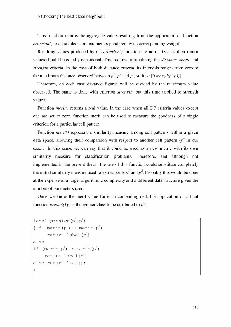
6 Choosing the best close neighbour
116
This function returns the aggregate value resulting from the application of function
criterion() to all six decision parameters pondered by its corresponding weight.
Resulting values produced by the criterion() function are normalized as their return
values should be equally considered. This requires normalizing the distance, shape and
strength criteria. In the case of both distance criteria, its intervals ranges from zero to
the maximum distance observed between p1, p2 and px, so it is: [0 max(d(px,p))].
Therefore, on each case distance figures will be divided by the maximum value
observed. The same is done with criterion strength, but this time applied to strength
values.
Function merit() returns a real value. In the case when all DP criteria values except
one are set to zero, function merit can be used to measure the goodness of a single
criterion for a particular cell pattern.
Function merit() represent a similarity measure among cell patterns within a given
data space, allowing their comparison with respect to another cell pattern (px in our
case). In this sense we can say that it could be used as a new metric with its own
similarity measure for classification problems. Therefore, and although not
implemented in the present thesis, the use of this function could substitute completely
the initial similarity measure used to extract cells p1 and p2. Probably this would be done
at the expense of a larger algorithmic complexity and a different data structure given the
number of parameters used.
Once we know the merit value for each contending cell, the application of a final
function predict() gets the winner class to be attributed to px.
label predict(p1,p2)
{if (merit(p1) > merit(p2)
return label(p1)
else
if (merit(p2) > merit(p1)
return label(p2)
else return lmaj();
}

6 Choosing the best close neighbour
117
Fig 6.4 Function that predicts the label class for a new query px.
Trie-Class always assign a class to each new object under scrutiny. The majority class
is attributed in the default case, on the condition that one of the two cell patterns p1 or p2
actually exhibit this class (which in the case of datasets with more than two classes
might not be true). If it is not, the pattern holding the criterion with the largest weight
value will be chosen instead.

6 Choosing the best close neighbour
118

119
7 Implementation
7.1 General overview
The drawing in Fig.7.1 shows the general idea on how Trie-Class algorithm is
implemented. There are three main steps in the construction of our classifier: pre-
processing data, building the required structures and running the classifier.
Fig 7.1 Trie-Class main modules
As every other algorithm learning by induction, Trie-Class begins by preparing the
training and test datasets. The training file will be used for “learning” and evaluating the
functioning of the algorithm. The test set is used once to finally classify unseen records.
Sample stratification, explained in Section 4 is used to obtain these subsets.
Original dataset
Training dataset
Dictionary
Test dataset
supportdata
Trie-Class
Stratify working files
Tree build
Parameter tuningEvaluation
set
Classifier
Results

7 Implementation
120
All attribute records within these files are discretized. This discretization is done
using interval values specified on the dictionary file for each attribute. In practice, in
many cases of domains with small number of values, the discretization process does not
alter the original values of an attribute and hence no domain compression takes place.
For instance consider the famous Cancer dataset, which consist of 10 attributes, all with
identical numeric domain values ranging from 0 to 10. If decided by the user, indicating
an interval of 1 for each domain in the dictionary file would produce this effect.
Trie-Class can handle missing values in categorical attributes if they form part of the
allowable values of an attribute.
Watching at the diagram it can be observed that the storage of records is not “ lazy” , a
characteristic of many instance-based methods.
Trie-Class uses a trie as tree structure to hold cell information, which will be used as
patterns at classification time. This tree structure does not hold training data on its
original format. C-trie keeps count on cell frequencies within each attribute interval.
These frequencies are used by the frequency DP criterion as explained earlier in Section
6. Besides this tree, a second file is created, which contains supporting information
needed by the algorithm. Basically it contains information on semi-exclusive intervals,
as defined in Equation (3.22) by function semk(), as well as information on joint
probability values for each symbolic attribute, needed for the distance calculations of
symbolic attributes as stated in Definition 26 and Equation (4.2). As for the first type of
information the file contains orderly lists of attributes. For each of them the file stores
those intervals where the semi-exclusive property holds. As it was explained in
Definition 19 in Section 3.4, the value of parameter φ is user-defined.
These two files appear labelled in Fig. 7.1 as “ Trie” and “ supporting data”
respectively.
A dictionary permanently loaded into main memory during tree construction and
classification completes the information for Trie-Class to work. It includes attribute
information: data type, interval size, maximum and minimum values and a class flag.
(For a complete layout of the dictionary see Annexe I).
In order to assign weights to decision parameters, Trie-Class divides the training set
itself into training and evaluation sets with approximately 80 and 20% of records
respectively. Decision parameters are tested against this last subset in order to decide

7 Implementation
121
the weight to assign to each decision parameter. This last sub-process is iterative as
depend on prediction error results, as suggested by the arrow pointing to itself in the
parameter tuning process of Fig. 7.1. Once decision parameters have their weights the
classification algorithm is ready to run against test data.
In the rest of this chapter, we explain tree growing, its characteristics, related work
and the search process. Finally, we argue that our search algorithm using best sub-cells
to obtain p1 when compared with regular k-NN methods as the sole decision criterion
increases classification accuracy and decrease execution time.
7.2 Building a trie as the main tree structure
A fundamental and very well studied technique for storing and retrieving data is to
use m-ary trees, also known as digital trees, lexicographic trees or simply tries, which
is its most widespread name and the one we use in this thesis.
Tries were first proposed in [de la Briandais, 1959] although the term trie, taken
from information retrieval has been given by [Fredkin, 1960]. Tries are used to store
multimedia images, web pages, string matching, remote sensing imagery, genetic
sequences, etc using all kind of trie variations: Patricia trees [Morrison, 1968], Two-
tries [Aoe, 1996], Triangulation tries [Bergman, 1994], R-trees [Guttman, 1984],
Quadtrees [Samet, 1984], Burst Tries [Heinz, LC-tries [Nilsson, 1999], among several
others.
Along the paths of the tree these structures do not store data at the nodes, which is
usually the case in regular trees. In a trie a set of strings from an alphabet containing m
symbols is stored in a natural way in an m-ary tree where each string corresponds to a
unique path. Branching at the jth level is determined by the value of the jth element from
the key. There are two types of nodes in a trie: branch nodes containing only pointers to
a number of children and leaf or element nodes, containing the string or key. Leaves
have no children. The root of the trie contains disjoint index values representing the first
letter or element of the string. At index position i, the pointer to the next letter points to
the sub-tree of all words starting with that letter. A pointer to the jth character of a key is
located at the jth level of the trie. All words containing a common prefix are located in
the same path represented by the various node levels. Trie structures represent
incomplete trees. Its leaves are not at the same level as shown in Figure 7.2.

7 Implementation
122
1 A B C .. .. Z v1 v2 v3 .. .. vn
0 A B … P ... R ... Z v1 v2 v3 vi .. vh .. vn
Fig. 7.2 Example of a classical trie after insertion of words
A leftmost binary field is sometimes used as a leaf indicator; a bit 0 indicates a leaf
node; otherwise a branch node. Our own tree structure is show next in Fig. 7.3.
Fig. 7.3 Section of C-trie showing 3 equal domain attribute levels
This structure slightly differs from the classical trie structure.
1 A B C .. .. Z v1 v2 v3 .. .. vn
[0] [1] [2] [3] [4] [5] [6] [7] [8] [9] Info 92 12 16 14 16 10 9 8 1 16 194
A * * * B B B * B B * 1 48 74 9 83 91 102 28 441 35 0
[0] [1] [2] [3] … [8] [9] 6 2 2 1 … 1 12
A A * B … B * 115 … 9
[0] [1] [2] … [9] 1 11 14 … 16
A * B … * 45 … 10
[0] [1] … [6] … [8] .. 1 … 1 … 1 3
2 … 4 … 2 *
… 45
[0] [1] [2] [3] [4] [5] [6] [7] ... 1 2 4 3 1 2 1 14 2 4 4 * 4 4 4 * 10
CAB
CAP CAR
Attribute 2
Attribute 1
Attribute 3

7 Implementation
123
From Equation (3.6) we know that each attribute value belonging to a record’s
sequence is converted into an integer value that we call cell component vi. Its value
ranges from 0 to si, which corresponds to the attribute’s domain.
It is using the vi component values from a cell vector p that the tree is built. Each cell
component value serves as the branching factor. This structure is permanently stored in
secondary memory. We call this tree the C-trie. As shown in Figure 7.3, every node in
the C-trie is formed by an array of j attribute interval values corresponding to cell
component value vi. Like regular tries, C-trie is also a kind of deterministic finite
automaton (DFA) [Cohen, 1990].
All input cells are n dimensional vectors. For this reason and contrary to normal tries
C-trie contains a fixed number of levels, one for each of the n attributes in the cell
vector. It also has no leaves, the last level corresponds to level n. The ith tree level
corresponds to the ith cell component value vi. Classes are not stored at leaves as is the
case with decision trees. They are indicated at each index positions within a node. In the
example of Fig 7.3 there are two classes A and B.
With the exception of the root node, all nodes in a level are linked together by
pointers forming n linked-lists, thus making easier to travel along that level. Cells
within each node have a record structure containing three pieces of information: a
counter field ctr holding sub-cell frequency, a class flag indicator, and a pointer ptr to
the next cell element down the tree. The class flag keeps track of sub-cell’s class
membership in a sort of “binary” fashion. As long as one or more identical sub -cells qi
from Equation (3.12) exhibits the same class, that class appears in the flag field at the ith
level. When a new cell p comes along for insertion, and its class c is different from the
existing one at qi, then the flag field becomes undetermined class-wise at sub-cell qi, a
fact marked with a ‘*’ in the flag field. For instance, for interval 0 on the root node
correspond a frequency of 92, a class “A” and pointer address of 1 pointing to next
node. This means a unique class exists for this full cell throughout the dataset. However,
for interval 1 with frequency 12, the class is ‘*’, meaning that two or more sub -cells
relate to two or more different classes. At some point along the cell path the class flag
becomes associated with one class only. This corresponds to a cell strength defined in
Equation (3.21). Every node contains an extra cell at the end of the array. It holds the
sum of cell frequencies in a node, the general class observed in the entire partition and a

7 Implementation
124
pointer to the next node of the same level. For instance in level 3, the leftmost node
points to node number 45, the next node at the same level. This number coincides with
the value of the pointer used by interval 2 in the rightmost node of level 2.
As is the case with other trees, such as the optimised kd-tree [Friedman et al, 1977]
C-trie recursively subdivides the nth-dimensional space using hyper planes orthogonal to
the coordinate axes.
Fig. 7.4 Overlapped class regions in a two-dimensional space.
As one descends along any tree path, sub-cell cardinality decreases very rapidly. In
the last level, it represents the number of identical cells p existing in the whole training
file. Keeping track of frequencies can be very useful in determining isolated sub-cells
that could result into outliers. Also, a map of frequencies like this can be useful to create
clusters of similar cell prefixes, a task that comes almost naturally with the structure of
tries.
An original contribution of Trie-Class with respect to the spatial class distribution is
its ability to keep track of cell class membership at the sub-cell level. Overlapped and
non-overlapped class areas are exactly mapped as shown in the example of Fig. 7.4 for
two-dimensional data. In simple terms, overlap is the data space region covered by sub-
cells where function nlabels(qi) > 1 (see Definition 16 and Equation 3.20b) Example
7.1, illustrate the same with vectors of numeric value.

7 Implementation
125
Example 7.1
Imagine we insert into a trie cell p1 = <3,1,1,1,3,”A”> with class “A” as shown in
Fig.7.5 (a). A second cell p2 = <3,1,1,3,2,”A”> is inserted next in 7.5(b) also with the
same class. In 7.5(c) a cell p3 = <3,1,1,7,4,”B”> is introduced.
Sub-cell q3 = <3,1,1, u> becomes immediately overlapped. By this we mean that
from the point of view of classes, two classes “share” the same prefix.
(a) (b) (c)
Fig. 7.5 Overlap class regions in the hyperspace
From sub-cell q4 onwards, sub-cells are associated with just one class, which
correspond to class “A” in the case of cells p1 and p2 and “B ” in the case of cell p3.
The information contained in these overlapped and non-overlapped class distribution
regions is used for class assignment of new instances.
7.3 Insertion algorithm
Trie-Class creates its trie incrementally as described next in Table 7.1.
3
1
1
1
3
3
1
1
1
3
3
2
3
1
1
1
3
3
2
7
4
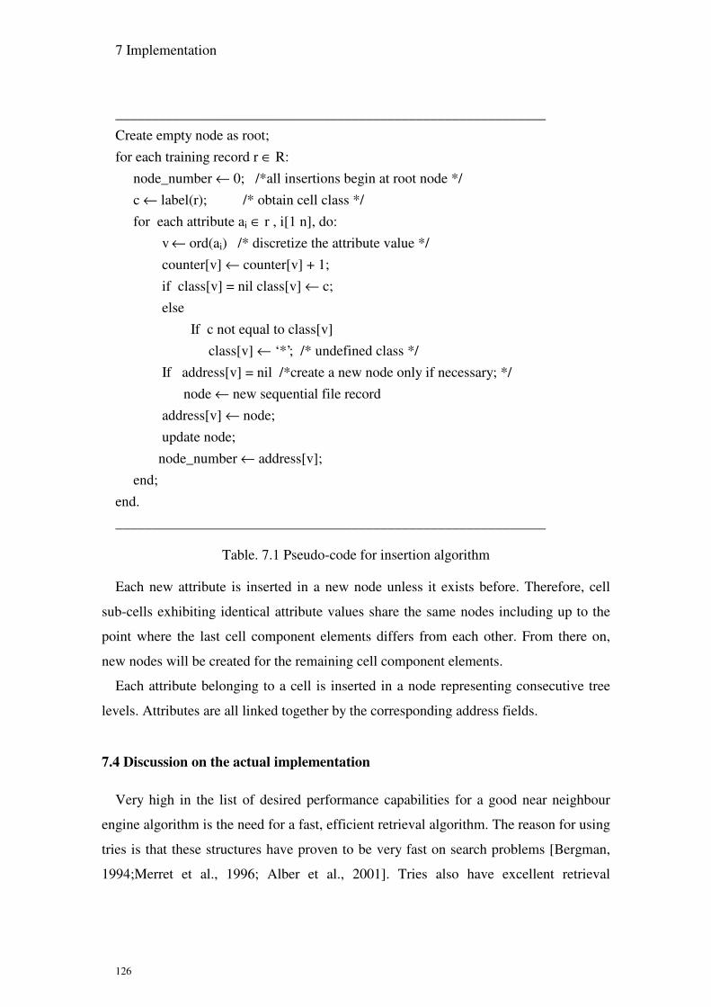
7 Implementation
126
____________________________________________________________ Create empty node as root; for each training record r ° R: node_number � 0; /*all insertions begin at root node */ c � label(r); /* obtain cell class */ for each attribute ai ° r , i[1 n], do: v � ord(ai) /* discretize the attribute value */ counter[v] � counter[v] + 1; if class[v] = nil class[v] � c; else If c not equal to class[v] class[v] � ‘*’; /* undefined class */ If address[v] = nil /*create a new node only if necessary; */ node � new sequential file record address[v] � node; update node; node_number � address[v]; end; end. ____________________________________________________________
Table. 7.1 Pseudo-code for insertion algorithm
Each new attribute is inserted in a new node unless it exists before. Therefore, cell
sub-cells exhibiting identical attribute values share the same nodes including up to the
point where the last cell component elements differs from each other. From there on,
new nodes will be created for the remaining cell component elements.
Each attribute belonging to a cell is inserted in a node representing consecutive tree
levels. Attributes are all linked together by the corresponding address fields.
7.4 Discussion on the actual implementation
Very high in the list of desired performance capabilities for a good near neighbour
engine algorithm is the need for a fast, efficient retrieval algorithm. The reason for using
tries is that these structures have proven to be very fast on search problems [Bergman,
1994;Merret et al., 1996; Alber et al., 2001]. Tries also have excellent retrieval

7 Implementation
127
properties for spatial data when dealing with a large number of dimensions in datasets
[Aoe, 1996; Merret, 1996] as well as for approximate searching of similar objects such
as remote sensing images [Alber, 2001] or similar but not identical cells as do it here.
From the insertion algorithm of previous section, we see that only required nodes for
new sub-cells are created. In other words all cell prefixes shares the same nodes. This is
a characteristic of regular tries. Exploiting this overlap of paths near the root helps in
achieving some degree of natural compression, which depends on cells spatial
distribution.[Merret, 1996]. Additional compression in front of dataset with a large
number of dimensions, could be achieved by using compression schemes such as a
DAWG graph [Appel, 1988] or the double array TAIL presented by [Aoe, 1989] which
share all transition states, or using a single node to stack common cell prefixes [Aoe,
1996], [Andersson, 1994]. There are still several known mechanisms offered to
compress trie size such as Patricia trees [Gonnet et al., 1991], X-tree [Berchtold et al.,
1996] and Burst tries [Heinz et al., 2002] among others.
Nevertheless, all these compression schemes in our case would reduce even further
information on cells, already limited by discretization. Also, some of these compress
mechanisms require going through the input file more than once to achieve its purposes.
At this point, we want to remember the fact that our purpose is not perfecting trie
compression techniques, but to produce a simple, efficient and accurate classification
algorithm.
In any case, very large dimension datasets pose a space problem. If compression is
desired for these cases, it could be achieved by one of the following simple methods.
The first one would be splitting C-trie into sub-trees holding different index ranges,
although this might influence I/O access time. The second and more important would be
to compress the first levels of the tree up to the point where sub-cells become associated
with classes, leaving all remaining suffixes in some linked list. Although this operation
would require processing a second time the training file, tree size would be smaller.
Suffix elements could also be keep in remaining common nodes.
Perhaps the best alternative would be creating a forest of trees each one holding only
cells of the same class. Each structure would represent the spatial distribution of one
class in the total data hyperspace. Searching the closest elements in these trees would be
carried on each tree using the same method as the one we use in Trie-Class. Several

7 Implementation
128
small subsets of close neighbours each belonging to one class would participate in the
final selection process using decision parameters. In these trees, equal binning
discretization method would have no importance whatsoever in terms of information
loss. It remains to see the time complexity of such forest structure.
Mixing strategies for tries is not new as a mean to balance its fast searching
capabilities with a large space usage [Knuth, 1997]. In both cases though, searching for
identical or similar cells would increase search time costs by introducing sequential
search mechanisms in these “big” nodes or linked lists. Compression techniques seem to
be consistent with the fact that the most relevant attributes are indeed first located into
the tree and these common prefixes are indeed strong representatives of the correct
mapping between cells and classes.
The search process described in Section 3.7 is constant and independent of the size of
the training file, a very important factor. This search process could be also considered as
searching in an ordered file as a matrix of i rows and j columns, with the search done on
columns represented by the ordered array of nodes, as is the case with some algorithms
such as [Micó, 1996]. The search is done starting from the ith column corresponding to a
given element value in a circular way increasing the radius each time by one unit,
looking each time to the next elements [i+1] and [i –1] discarding all others as soon as
an existing cell value is found. For this reason algorithm’s complexity is constant and
equal to 2(log n) on the average case.
Search time is always constant in Trie-Class, unless used the “ look ahead”
mechanism. Search complexity is logarithmic, if we use total nodes visited as a measure
of complexity, as done in other cases [Yanilos, 1993].
Keeping the count of frequencies at sub-cell level allows us to have a graphical
distribution of cell density. This not only helps in breaking ties when selecting
neighbour elements within a given node, as it could be used to extend the use of this
structure for clustering as well [Anderberg, 1973].
Search time is fast in C-trie. Taking advantage of array indexing, for any given index
value j we look for existing cell values to the “left” starting at j, j-1,..0, and to the right
starting at j+1 within interval [1..i]. Once cell(s) found within the node, we eliminate
from the search the rest of the tree, concentrating in the following sub-tree. This is
equivalent to take into account the triangle inequality [Burkhard, 1973] to significantly

7 Implementation
129
reduce the number of direct distance calculations needed for an efficient search
algorithm as in [Berman, 1999]. The search phase is done in O(ni) time complexity.
Trie-Class can learn, due to the fact that is persistent. New training cells can be easily
added. Record deletion is more complicated but is not considered as a functional part of
the algorithm. Changing the training file is interpreted as growing again a new tree.
It should not be neglected the fact that C-trie was designed to hold a sample from the
database, whose only requirement is to be representative of the data in the statistical
sense. This means that most of the time we are dealing with a manageable number of
records.
Although the actual structure for prototyping is done using dynamically sized arrays
for every node, linked lists could also be used to save array size in sparse distributions.
As it is well known, this structure unless indexed, has a drawback of a sequential search.
Alternatively, hashing tables containing internal node indexes could also be used, but
constructing them requires also extra time.
7.5 Dictionary and other supporting files
Like many other data mining applications, ours also use a user-provided dictionary
file. Basically it contains information on all attributes, the type of data, i.e. numeric
discrete, continuous or symbolic, the minimum and maximum possible values they can
take (their domain), the size of the interval to be used as a domain partition in the tree
structure and a flag indicating whether this is the class field or not.
An example of the dictionary can be found in the Appendix I.
It is worth saying at this point that with an extra single read of the training sample
most of this information could be automatically detected. The only requirement to be
supplied by the user would be the size of the interval for each attribute. This information
is crucial for tree construction, and allows the user adjust algorithm efficiency by
altering the interval for whichever attribute. This user interface with the software is very
important for all classification algorithms in data mining, where to a large degree they
play a key role in the success of the end result. There is nothing compared with this
knowledge, if such knowledge exists, and cannot be overlooked with the obsession of
automation.

7 Implementation
130
Along with C-trie and dictionary files Trie-Class uses a couple more of files
containing information devoted to two different purposes.
One of them is to keep information on semi-exclusive intervals as defined in Equation
(3.22), which is basically an ordered table keeping for each attribute and partition
interval, values which relate to one class only. These are sometimes called “pure
attributes” [Breiman, 1984] or “primary ” [Turney, 1996] in the literature. These
attributes are informative of the class when considered by themselves [Kohavi, 1997].
Optionally, the user can decide to have this file information somehow softened: the
information contains interval values for those attributes where one of the classes holds a
user-defined threshold percentage of the number of training cells. Whichever the degree
of exclusiveness is selected, this file is used at generalization time when cell values are
checked for the presence of one or more of these values.
A second file, also on disk is used to keep information on symbolic attributes
frequencies. For each symbolic attribute the file keeps one record for each class
containing the frequency of each value. These are used in the distance calculation for
these types of attributes, specifically in the calculation of the joint probability P(v�c)
already explained in Section 4.2.
These two files appear under the name “support data” in the diagram of Fig. 7.1.

131
8 Conclusions and Future work
In this dissertation, we explored specific paradigms for data classification, namely,
decision trees and instance-based methods in an effort to develop an experimental
algorithm able to improve some of its aspects while simplifying algorithmic complexity.
The order of the conclusions presented here is arbitrary with respect to its importance
degree. Rather, we have followed the sequential order in which these topics appear on
this work.
There are literally dozens of algorithms to solve classification problems in the
literature. Our approach was in general to keep it as simple as possible, considering the
truthfulness of the well-known paradigm of the Minimum Description Length principle.
Within this context we did retain two of the more popular methods, instance-based and
decision trees as inspiration to develop our own. From the first one we took the main
idea of not using a central model developed to classify all records – as done for instance
in decision trees - but to use training records themselves as patterns to locally represent
on each case the best model to assign its class to some unknown query. From the second
of these methods, we have taken the idea of using a tree to store actual records as a
means of rapidly searching records in the data hyperspace. This is as far as it goes the
similarity between our algorithm and decision trees because in this kind of paradigm
tree nodes are used as threshold decision values that together represent a general model
used to classify in the same manner all test records. In our case, the use of a trie serves
only the purpose of an index with very fast access, but not as a generator of a
classification model. In fact our algorithm in this respect has a totally opposed
behaviour to decision trees and it is similar to the nearest neighbour method.
Trie-Class use a simple algorithm overall, formed by small contributions along the
various phases of the Data Mining process.
• The development of the concept of sub-cells, as a method for early class
identification as well as pattern characterization for model selection (Section
3.3).
• A sub-optimal search method for the extraction of near neighbours, different
from the traditional distance calculation, which gives elimination power to
more relevant attributes (Section 3.7).

8 Conclusions and Future work
132
• A simple mechanism to differentiate relevant and non-relevant attributes using
a one-dimension projection of attribute values and semi-exclusive intervals
(Section 4.3).
• The use of joint probabilities to solve the distance calculation problem in the
presence of symbolic attributes (Section 4.2).
• The use of Decision Parameters in the final pattern selection process uses
concepts such as cell strength, semi-exclusivity and shapes (Section 6.1).
These parameters enrich the information about objects. By having a weight
according with training data characteristics (Section 6.3), they adapt the
algorithm to the data under inspection.
8.1 Conclusions
Our experimental results from Section 5 show that on average Trie-CLASS performs at
least as good as several of the leading classifiers reported, whether this comparison is
done against classifiers running in our test bench or whether we compare with results
found in the bibliography18. In particular this is true with respect to the landmark
classifier C4.5 [Quinlan, 1986] and the instance-based learning k-NN algorithm [Aha,
1991]. In eleven out of thirteen files compared against C4.5, ours was better. It also
appears clear from these figures that Trie-Class performs equally well with various
types of data, numeric or symbolic as well as average dataset sizes and dimensions. Our
figures also show that Trie-Class has poorer results when the number of classes is
greater than two, perhaps due to the fact that the actual algorithm is only implemented
to extract two cell patterns representing two different classes.
A clear improvement over regular NN methods is the search mechanism used to
extract selected records using a greedy strategy. Trie-Class extracts near objects using
the concept of similarity in turn assimilated to a distance calculation. Its searching
method restricts the search area within the trie according with previous values found at
sub-cell levels, thus avoiding the visit to all unnecessary tree branches. The extraction
of additional cells restricts even further the search space, as its class must be different
18 As new results on classifiers performance appear every day in the literature, some of our figures could be out of
date.

8 Conclusions and Future work
133
from the class of the previous cells extracted. Overall, reduced areas of the data space
are searched to obtain close neighbours.
Greedy search strategies are in general sub-optimal, as they can loss better solutions.
The counter part to this been that some complex algorithmic problems can find some
acceptable solution. Our results, mixing a greedy search with look-ahead for ties
situations prove to be encouraging. In fact, Trie-Class obtain better results than IBk, a
Weka implementation of a k-NN algorithm, when the value of k = 1.
Feature subset selection is the process of identifying and removing as much irrelevant
and redundant information as possible. Searching the feature space within reasonable
time is necessary, especially for the case o data with large number of features. For this
reason reducing data dimensionality is dealt using a heuristic search strategy as opposed
to an exhaustive search of the feature space prohibitive most of the time. They are more
feasible and can give good results, although they do not guarantee finding the optimal
subset. Regularities on data are found in Trie-Class using every other feature one at a
time, independently from others using a previously discretized single-dimension space.
Using this criterion attributes can be ordered by degree of relevance, allowing the
removal of irrelevant values without diminishing severely classification accuracy.
Feature selection is done before tree growth. Most relevant attributes produce the initial
data space divisions and thus most similar objects remains close, a problem affecting
several classification algorithms. This fact also influences distance calculation, because
more elimination power is given to more relevant attributes largely reducing the search
space.
We have already said that Trie-Class extracts two near cells as a first approximation
to classify new objects. In a next step it uses a “voting” mechanism to make a final
decision that is different from all other k-NN algorithms we know of. This selection is
done through the use of decision parameters, which allow the extraction of further
information from pre-selected cell patterns. This represents richer knowledge about
these competing neighbours, a procedure that goes beyond the standard mechanism of
using distance as the sole criterion. Moreover, decision parameters are weighted
according with its ability to classify new records, dynamically adapting the whole
algorithm to the changing characteristics of data. This adaptation of the algorithm
constitutes an important step towards fighting the known fact that not all classification

8 Conclusions and Future work
134
algorithms performs equally well with different datasets. We have no knowledge of
these technique been used before.
Distance calculation for symbolic attributes constitutes a problem of its own, dealt in
different ways by different authors. Trie-Class uses a heterogeneous mechanism
depending on the type of value (discrete, continuous or symbolic). In the specific case
of symbolic attributes it uses a simple mechanism of low complexity based on the joint
probability distribution of classes within attributes and its corresponding values,
resembling somehow the functioning of Bayesian Networks at a given node. This
mechanism works better than the simple overlap solution and is cheaper in complexity
than more sophisticated methods.
The choice of using a multi-way tree indexed on attribute values works as a very fast
index and we believe it is a good solution for the type of search carried on. It has been
demonstrated that this structure allows a very fast search and presents a low
computational complexity for the required type of proximity search [Bentley, 1997] as
well as in the case of large multimedia databases. Contrary to standard tries, useful
information represented by records class membership is not found at tree leaves but at
each tree level, i.e. associated with sub-cells, allowing the drawing of a very useful class
map in the data space. Moreover, difficult choices of threshold values as in the case of
decision trees are avoided.
In this structure search time is independent of the file size and exhibit low algorithmic
complexity, a problem found in many search methods as our results show with respect
to execution time.
The gain we obtain with a fast search has the cost of sometimes using a larger disk
space, as our data structure is disk resident. As disk space has sky rocketed in terms of
capacity, and at the same time with systematic decreasing prices and increasing access
speeds in the last decade, our choice seems to be adequate. In any case, the eventual use
of pruning at the level of sub-cells or prefixes belonging to a single class can diminish
easily tree size, not to mention the fact that Trie-Class requires only a representative
sample not the entire population in order to classify and thus the size of the required
structure is always under control. The algorithm implemented by Trie-Class can be
alternatively implemented using any database management system. This could simply

8 Conclusions and Future work
135
handle all required data and carry the search mechanism using some of the existing
database techniques.
8.2 Future work
Trie-Class extracts two near neighbours in order to select the class of one of them as
the class to assign to a new query object. In this respect, as a proposal for further work,
an obvious way of decreasing tree size and perhaps improve classification accuracy in
datasets with more than two classes, would be the use of a forest with as many trees as
classes exist in a given dataset. Each one of these trees would hold records belonging to
one class only. At search time the actual search algorithm would be used to extract one
or two cell patterns per tree, each one of them associated with a single class.
Trie-Class tree structure called C-trie allows the identification of classes at the sub-
cell level. Manipulating this map of classes would allow a graphical representation of
clusters of classes and its frequencies.
Clustering techniques could be easily implement with Trie-Class, an aspect in Data
Mining that was out of the scope of this work. As clusters represent objects with
common characteristics, all six decision parameters are a good solution to identify these
common objects, especially applied at sub-cell levels. The application of these criteria
would extend the use of distance as the sole similarity criterion used in many clustering
algorithms, allowing a richer similarity concept and thus allowing the selection of
clusters with a strong internal strength. In this sense, Trie-Class can become a bivalent
tool, allowing the implementation of classification as well as clustering techniques.
One of the decision parameters used to select the best representative pattern is shapes,
a vector of values representing inter-attribute relationships, which are used to identify
pattern similarity. Considering the encouraging results of this decision parameter in
classification, it would be worth investigating further the possibility of creating a whole
new metric space using this shape criterion.
Finally, another aspect not implemented in this thesis is the fact that we use decision
parameters and the merit() function as a mean of selecting the most representative cell
pattern. We could well substitute the original search mechanism to extract near
neighbours all together and replace it by the value provided by this function. Thus, it
would be used to define a new similarity metric. This might represent a richer similarity

8 Conclusions and Future work
136
concept if compared with the use of distance as the only similarity criterion between
objects.

137
9 Bibliography
Agarwal, P., Erickson, J., 1999. Geometric range searching and its relatives, Advances in Discrete and Computational Geometry, Contemporary Mathematics 223, American Mathematical Society Press, pp. 1-56.
Agrawal, R., Imielinski, T., Swami, A., 1993. Mining Association Rules between Sets of Items in Large Databases, Proceedings of the ACM International Conference on Management of Data, pp. 207-216.
Aha, D. W., Kibler, D., Albert, K., 1991. Instance-Based Learning Algorithms, Journal of Machine Learning, Vol. 6, pp.37-66
Aha, D. W., 1992, Tolerating noisy, irrelevant and novel attributes in instance-based learning algorithms, International Journal of Man-Machine Studies, Vol. 36, pp 267-287.
Aha, D. W, Bankert, R., 1994. Feature Selection for Case-Based Classification of Cloud Types: An Empirical Comparison, In D.W. Aha (Ed.) Case-Based Reasoning: Workshop (Technical Report WS-94-01, CA, AAI Press.
Aha, D. W., Bankert, R., 1995. A comparative evaluation of sequential feature selection algorithms, Proc. of the Fifth Intl. Workshop on Artificial Intelligence and Statistics, pp., 1-7.
Alber, I. E., Xiong, Z., Yeager, N. , Farber, M., Pottenger, 2001, W. M. Fast Retrieval of Multi-hand Hyperspectral Images Using Relevance Feedback. Proceedings of the International Geoscience and Remote Sensing Symposium, Vol 3, pp 1149-1151.
Anderberg, M.R., 1973. Cluster Analysis for Applications. Academic Press, N.Y., USA.
Andersson, A, Nilsson, S., 1993, Improved behaviour of tries by adaptive branching. Information Processing Letters, Vol. 46, pp. 295-300
Andersson, A, Nilsson, S., 1994, Faster Searching in Tries and Quad trees – An Analysis of Level Compression, in Proceedings of the Second European Symposium on Algorithms, pp. 82-93.

Bibliography
138
Aoe, J., 1989. An Efficient Digital Search Algorithm by Using a Double Array Structure, IEEE Transactions Software Engineering, Vol 15:9, pp. 1,066-1,077.
Aoe, J, Katsushi, M., Shishibori, M., Park, K., 1996. A trie compaction algorithm for a large set of keys, IEEE Transactions on Knowledge and Data Engineering, vol. 8, nº 3, pp. 476-491.
Appel, A.W., Jacobson, G.J., 1988. The World’s Fastest Scrabble Program, Communications of the ACM, Vol 31:5, pp. 572-578.
Arya, S., Mount, D. M., Netanyahu, N. S., Silverman, R. Wu, A., 1998. An optimal algorithm for approximate nearest neighbor searching, Journal of the ACM, 45(6), pp.891-923.
Aurenhammer, F., 1991. Voronoi diagrams – a survey of a fundamental geometric data structures, ACM computing surveys '91 (Japanese translation), Kyoritsu Shuppan Co., Ltd., pages 131-185.
Baeza-Yates, R., Cunto, W., Manber, U. Wu, S., 1994. Proximity matching using fixed-queries trees. In Proc. 5th Combinatorial Pattern Matching (CPM 94), Lectures Notes in Computer Science, Nº 807, pp. 198-212.
Batchelor, B. G., 1978. Pattern Recognition: Ideas in Practice. New York: Plenum Press, pp. 71-72.
Beckmann, N., Kriegel, H, P., Schneider, R., Seeger, 1990. B., The R*-tree: An efficient and Robust Access Method for Points and Rectangles, Proc. ACM SIGMOD International Conference on Management of Data, Atlantic City, USA, pp. 322-331.
Bentley, J. L., 1975. Multidimensional binary search trees used for associative searching. Communications of the ACM, Vol. 18(9), pp. 509-517.
Bentley, J. L., 1980. Multidimensional Divide and Conquer, Communications of the ACM, 23(4), pp. 214-229.
Bentley, J. L., Sedgewick, R., 1997, Fast algorithms for sorting and searching strings. In Proc. of the Annual ACM-SIAM Symposium on Discrete Algorithms, New Orleans, USA, pp. 360-369.

Bibliography
139
Benzecri, J. P., 1992, Correspondence Analysis Handbook, Ed. Dekker, Marcel Inc., 688 pp.
Berchtold, S., Keim, d. A., Kriegel, 1996, H.P., The X-tree: An Index Structure for High-Dimensional Data, Proceedings of the 22nd. International Conference on Very Large Databases, Bombay, India, pp. 28-39.
Berman, A.P., 1994. A New Data Structure For Fast Approximate Matching, Technical Report, 1994-03-02, Dept. of Computer Science, University of Washington.
Berman, A. P., Shapiro, L. G., 1999, Triangle-Inequality-Based Pruning Algorithms with Triangle Tries. Proceedings of the IS&T and SPIE Conference on Storage and Retrieval for Image and Video Databases VII, San José, CA, USA.
Bin Liu, Y. Ma, and C.K. Wong, 2000. Improving an Association Rule Base Classifier, Principles of Data Mining and Knowledge Discovery, pp. 504-509.
Blanzieri, E., Ricci, F., 1999. Advanced Metrics for Class-Driven Similarity Search, International Workshop on Similarity Search, Firenze, Italy.
Bologna, G., 2001. A Study on Rule Extraction from Neural Networks Applied to Medical Databases, International Journal of Neural Systems, Vol. 11, No. 3 (2001) 247-255.
Bozkaya, T., Ozsoyoglu, M., 1997, Distance-based indexing for high-dimensional metric spaces. In Proc. ACM SIGMOD International Conference on Management of Data, pp. 357-368.
Breiman, L., Friedman, J., Olshen, R., Stone, C., 1984, Classification and Regression Trees, Wadsworth International Group.
Brighton, H., Mellish, C., 2002, Advances in Instance Selection for Instance-Based Learning Algorithms, Data Mining and Knowledge Discovery, 6, Kluwer Academic Publishers, The Netherlands, pp. 153-172
Brin, S., 1995. Near neighbor search in large metric spaces. In Proc. 21st. Conference on Very Large Databases (VLDB 95), pp. 574-584.
Brodley, C.E., 1995a, Recursive automatic bias selection for classifier construction. Machine Learning, Vol. 20, pp. 63-94.

Bibliography
140
Brodley, C.E. 1995b, Multivariate Decision Trees, Machine Learning, Vol. 19(1), pp 45-77.
Burkhard, W. A., Keller, R.M., 1973, Some approaches to best-match file searching, Communications of the. ACM, Vol. 16: 4, pp. 230-236.
Catlett, J., 1991, On Changing Continuous Attributes into Ordered Discrete Attributes, Lecture Notes in Artificial Intelligence, Ed. J. Siekmann, Springer-Verlag, Berlin, pp. 164-178.
Cha, M.Y, Gero, J.S., 1998. Shape Pattern Recognition Using a Computable Pattern Representation, Artificial Intelligence in Design, Kluwer Academic Publishers, pp. 169-187.
Chavez, E., Navarro, G., Baeza-Yates, R., Marroquin, J., L., 2001. Searching in Metric Spaces, ACM Computer Surveys, Vol. 33:3, pp. 273-321.
Chawla, N., Eschrich, S., Hall, L.O., 2001. Creating Ensembles of Classifiers, International Conference on Data Mining, ICDM, San José, CA, USA., pp.580-581.
Cheeseman, P., Stutz, J., 1995. Bayesian Classification (AutoClass): Theory and Results, in Advances in Knowledge Discovery and Data Mining, U. M. Fayyad, G. Piatetsky-Shapiro, P. Smyth, & R. Uthurusamy, Eds. The AAAI Press, Menlo Park, pp. 153-180.
Chmielewski, M. R., Grzymala-Busse, J.W., 1994. Global discretization of continuous attributes as preprocessing for machine learning, Third International Workshop on Roughs Sets and Soft Computing, pp. 294-301.
Ching, J. Y.,Wong, A.K.C. & Chan, K.C.C, 1995. Class-dependent discretization for inductive learning from continuous and mixed-mode data. IEEE Transactions on P.A.M.I., vol. 17, pp. 641-651.
Chou, Y., Shapiro, L. G. 2000. A Hierarchical Multiple Classifier Learning Algorithm, Proceedings of the Intl. Conference on Pattern Recognition, Vol. 2, pp. 152-155.
Ciaccia, P, Patella, M., Zezula, 1997. P., M-tree: an efficient access meted for similarity search in metric spaces., In Proceedings of the 23rd Conference on Very Large Databases (VLDB 97), pp. 426-435.

Bibliography
141
Cios, K., W. Pedrycz, R. Swiniarski, 1998. Data Mining Methods for Knowledge Discovery, Kluwer Academic Publishers, London.
Clement, J., Flajolet, P., Vallée, B., 2001. Dynamic sources in information theory: A general analysis of trie structures, Algorithmica, Vol. 29(1/2), pp.307-369.
Cohen, D., 1990. Introduction to Theory of Computing, John Wiley & Sons.
Collobert, R., Bengio, S., Bengio, Y., 2001. A Parallel Mixture of SVMs for Very Large Scale Problems, IDIAP Research Report, nº RR 01-12, Switzerland.
Cover, T. Hart, P. 1967. Nearest neighbor pattern classification, IEEE Transactions on Information Theory, Vol. 13:1, pp 21-27.
Dasarathy, B.V., 1991. Nearest Neighbor (NN) Norms: NN Pattern Classification Techniques, IEEE Computer Society Press, Los Alamitos.
Dehne, F., Nolteimer, H., 1987. Voronoi trees and clustering problems, Information Systems Nº12(2), pp 171-175.
De la Briandias, R., 1959. File searching using variable length keys. In Proc. Western Joint Computer Conference, Vol. 15, Montvale, N.J., AFIPS Press.
De Mántaras, R., 1991. A Distance-Based Attribute Selection Measure for Decision Tree Induction, Machine Learning, Vol. 6, pp. 81-92.
Dijkstra, E., 1972. The Humble Programmer, Turing Award Lecture at the ACM Annual Conference, Boston, USA.
Doak, J., 1992. An evaluation of feature selection methods and their application to computer security, Technical Report CSE: 18, Davis, Dept. of Computer Science, U. of California., USA.
Domingo, C, Watanabe, O, 2000. Scaling up a boosting-based learner via adaptive sampling, in Proc. of Knowledge Discovery and Data Mining (PAKDD'00), Lecture Notes in AI 1805, 317-328.
Domingos, P, 1996. Unifying Instance-Based and Rule-Based Induction, Machine Learning, 24(2), pp.141-168.

Bibliography
142
Dougherty, J., Kohavi, R., Sahami, M., 1995. Supervised and Unsupervised Discretization of Continuous Features, Proceedings of the 12th Intl. Conference on Machine Learning, Morgan Kaufman Publ., San Fco., USA, pp. 194-202.
Duch, W., Grudzinski, K., 1998. Weighting and selection of features, Proc. of the Workshop Intelligent Information Systems VIII,�8VWUR���3RODQG����-18.06.1998, pp. 32-36.
Duda, R., O., Hart, P.E., 1973. Pattern classification and scene analysis, New York: John Wiley & Sons.
Duntsch, I., Gedida, G., 1998. Uncertainty measures of rough set prediction, Artificial Intelligence 106, pp.109-137.
ECML/2002, 2002. Thirteen European Conference in Machine Learning, Helsinki, Finland.
Efron, B., 1983. Estimating the error rate of a prediction rule: improvement on cross-validation, Journal of the American Statistical Association, 78(382), 316-330.
Efron, B., Tibshirani, R., 1993. An introduction to the bootstrap, Chapman & Hall, London.
Elder J. F., Abbott D. W., 1998. A Comparison of Leading Data Mining Tools, 4th
International Conference on KDD, N. York, USA.
Everitt, B. S. & Hand, D.J., 1981. Finite Mixture Distributions, Ed. Chapman and Hall, London.
Faloutsos, C., Lin, K., 1995. Fastmap: A fast Algorithm for Indexing, Data-Mining and Visualization of Traditional and Multimedia Datasets, Proceedings of the ACM SIFMOD International Conference on Management of Data, San Jose, CA, USA, pp 163-174.
Fayad, U., Kebi, I. 1992. On the Handling of Continuous-Valued Attributes in Decision Tree Generation, Machine Learning, Vol. 8, pp. 87-102.
Fayyad, U., Kebi, I. 1992. On the Handling of Continuous-Valued Attributes in Decision Tree Generation, Machine Learning, Vol. 8, pp. 87-102.

Bibliography
143
Fayyad, U., Irani, K. B., 1993. Multi-interval discretization of continuous-valued attributes for classification learning, Proceedings of the 13th International Joint Conference on Artificial Intelligence, pp. 1022-1027.
FCC, 2002. Federal Communications Commission News, Washington, USA, July 23th, 2002.
Fix, E. and Hodges, J.L., 1951. Discriminatory analysis, non-parametric discrimination. Technical report, USAF School of Aviation Medicine, Randolf Field, Tex. Project 21-49-004, Report. 4, Contract AF41(128)-31.
Flach, P. A., 2001. On the state of the art in Machine Learning: a personal review, Artificial Intelligence, 13(1/2): pp.199-222.
Flajolet, Ph., 1983. On the performance evaluation of extendible hashing and trie searching, Acta Informática Vol. 20, pp. 345-369.
Forbes Magazine, 2002. Monet launches high-speed wireless data network, Reuters, Oct. 29th, 2002.
Frawley, W., Batheus, C., 1991. Knowledge Discovery in Databases: An Overview. In Piatetsky-Shapiro, G. and Frawley, W. (Eds.), Knowledge Discovery in Databases, MIT Press, Cambridge, MA, pp1-27.
Fredkin, E. Trie Memory, 1960. Communications of the ACM, Vol.3:9, pp. 490-500.
Friedman, J.H., Bentley, J.L. Finkel, R.ª, 1977. An algorithm for finding best matches in logarithmic expected time. ACM Transactions on Mathematical Software 3:3, pp 209-226.
Garcke , J., Griebel , M., 2001. Classification With Sparse Grids Using Simplicial Basis Functions, Proc. of the the Seventh ACM SIGKDD International Conference on Knowledge Discovery and Data Mining, San Francisco, CA, USA, pp. 87-96.
Gehrke, J., Ganti, V., Ramakrishnan, R., Loh, 1999. W-Y., BOAT – Optimistic decision tree construction, Proceedings of the SIGMOD Conference, New York, USA: ACM Press, pp. 169-180.
Gennari, J. H., Langley, P., Fisher, D., 1989. Models of Incremental Concept Formation, Artificial Intelligence, Vol. 40, pp. 11-61.

Bibliography
144
Goldberg, D., 1989. Genetic Algorithms in search, Optimisation and Machine Learning, Addison-Wesley, Reading, MA., USA.
Goodman, R., P.J. Smyth, 1988. Decision tree design from a communication theory standpoint, IEEE Transactions on Information Theory, 34(5):979-994.
Grossman, R., Chandrika, K, Kumar, V., 2001. Editors, Data Mining for Scientific and Engineering Applications, Kluwer Academic Publishers.
Guttman, A., 1984. R-trees: A dynamic index structure for spatial searching, Proceedings of the ACM-SIGMOD Conference on Management of Data (1985), Boston, MA., USA, pp. 47-57.
Guyon, I., 2001. Introduction to the NIPS 2001 Workshop on Variable and Feature Selection, BC., Canada.
Hamming, R.W. 1973. Numerical Methods for Scientists and Engineers. McGraw-Hill.
Han, J., Kamber, M., 2001. Data Mining: Concepts and Techniques, Morgan Kaufmann, San Fco., CA., USA.
Hand D.J., Mannila H., Smyth P. 2001. Principles of data mining, MIT Press, Boston, MA.,USA.
Hansen, L., Salamon, P., 1990. Neural network ensembles, IEEE Transactions on Pattern Analysis and Machine Intelligence, Vol. 12, pp. 993-1001.
Heat, D., Kasif, S., Salzberg, S., 1993. Learning oblique decision trees, Proceedings of the 13th International Joint Conference on Artificial Intelligence, Morgan Kaufmann, France, pp. 1002-1007.
Heinz, S., Zobel, J., Williams, H.E., 2002. Burst Tries: A Fast, Efficient Data Structure for String keys, ACM Transactions on Information Systems, 20(2), pp. 192-223.
Hegland, M., Nielsen, O. M., Shen, Z., 2000. High dimensional smoothing based on multilevel analysis. Technical report, Data Mining Group, The Australian National University, Canberra, Submitted to SIAM Journal of Scientific Computing.

Bibliography
145
Holte, R. C., 1993. Very Simple Classification Rules Perform Well on Most Commonly Used Datasets, Machine Learning, Vol.11, pp. 63-91
Hunt, E., Marin, J. & Stone, P., 1966. Experiments in Induction, Academic Press Inc., New York, USA.
Indyk, P., 2000. Dimensionality Reduction Techniques for Proximity Problems, Proc. 11th ACM-SIAM Symposium on Discrete Algorithms, pp. 371-378.
ICDM 02, 2002. The “002 IEEE International Conference on Data Mining, Maebashi, Japan, December 2002.
ICML 2002, Nineteenth International Conference on Machine Learning, Sydney, Australia, July 2002.
John, G., Langley, P., 1996. Static Versus Dynamic Sampling for Data Mining, Proceedings of the Second International Conference on Knowledge Discovery in Databases and Data Mining, AAAI/MIT Press.
Johnson, R.A., Wichern, D. W., 1998. Applied Multivariate Statistical Analysis, Prentice-Hall, Forth Edition.
Kalantari, I., McDonald, G., 1983. A data structure and an algorithm for the nearest point problem, IEEE Transactions on Software Engineering, 9(5), pp. 631-634.
KDD 2002, Eight ACM SIGKDD International Conference on Knowledge Discovery and Data Mining, July 2002, Edmonton, Canada,
Kaski, S., 1997. Data exploration using self-organizing maps. Acta Polytechnica Scandinavica, Mathematics, Computing and Management in Engineering Series No. 82, 57 pp.
Kerber, R., 1992. ChiMerge: Discretization of Numeric Attributes, Proceedings of the 10th National Conference on Artificial Intelligence, pp 123-127.
Knuth, D., 1998. The Art of Computer Programming, Vol. 3, Sorting and Searching, Reading, Massachusetts: Addison-Wesley, 1998, MA., USA.
Kohavi, R., 1995. A Study of Cross-Validation and Bootstrap for Accuracy Estimation and Model Selection, Proceedings of the Fourteenth International Joint

Bibliography
146
Conference on Artificial Intelligence, San Francisco, CA, USA: Morgan Kaufmann, pp. 338-345.
Kohavi, R., 1996. Scaling Up the Accuracy of Naive-Bayes Classifiers: a Decision-Tree Hybrid, Proceedings of the Second International Conference on Knowledge Discovery and Data Mining, Edited by E. Simoudis, J. Han, and U. Fayyad, The AAAI Press, pp. 202-207.
Kohavi, R, John, G., 1997. Wrappers for Feature Subset Selection, Artificial Intelligence Journal, Special issue on relevance, Vol. 97, Nº 1-2, pp 273-324.
Lachlan, R. 1983. The Principle of Continuity." §8 in An Elementary Treatise on Modern Pure Geometry. Ed. Macmillian, London, pp. 4-5.
Langley, P., 1996. Elements of Machine Learning. Morgan Kaufmann.
Lebowitz, M., 1985. Categorizing Numeric Information for Generalization, Cognitive Science, Vol. 9, pp. 285-308.
Lee, D.T., Preparata, F.P., 1984. Computational geometry- A Survey, IEEE Transactions on Computers, Vol. C-33: 12, pp. 1072-1101.
Lesh, N., Zaki, M., Ogihara, M. 1998. Mining Features for Sequence Classification, MERL Technical Report Number: TR98-22.
Li, J., Dong, G., Ramamohanarao, K., 2000. Instance-Based Classification by Emerging Patterns, Proceedings of the Fourth European Conference On Principles and Practice of Knowledge Discovery in Databases, Springer-Verlag, pp. 191-200.
Lin, S. -K., 2001. The Nature of the Chemical Process. 1. Symmetry Evolution –Revised Information Theory, Similarity Principle and Ugly Symmetry. International Journal of Molecular Sciences, vol. 2, pp.10-39.
Liu, B., Ma. Y, Wong, C.K, 2000. Improving an Association Rule Based Classifier, 4th European Conference on Principles and Practice of Knowledge Discovery in Databases, Lyon, Springer-Verlag, pp. 504-509.
Lohr, S. L., 1999. Sampling: Design and Analysis, Duxbury Press, Brooks/Cole Publishing Co., CA, USA.

Bibliography
147
Lyman, P., H. R. Varian, 2002. Report: How Much Information. Available from http://www.sims.berkeley.edu/how-much-info on June 2002. School of Information Management and Systems, University of California, Berkeley, CA, USA.
Mangasarian, O. L., Wolberg, W. H., 1990. Cancer diagnosis via linear programming", SIAM News, Volume 23, Nº 5, pp. 1-18.
Mehrotra, R.. Gary, J. E., 1995. Similar-shape retrieval in shape data management. IEEE Computer, 28(9): pp. 57-62.
Meretakis, D., Lu, H., Wuthrich, B., 2000. A study on the performance of Large Bayes Classifiers, 11th European Conference on Machine Learning, Catalonia, May 30-June 2, Spain.
Michalski, R., Mozetic, I., Hong, J., and Lavrac, N. 1986. The multi-purpose incremental learning system AQ15 and its testing application to three medical domains. Proceedings of the 5th National Conference on Artificial Intelligence, Philadelphia, Morgan Kaufmann 1041-1047.
Michalsdi, R., Tecuci, G., 1994. Proc. of the Second International Workshop on Multi-strategy Learning, harpers Ferry, Va: Office of naval research/G. Mason University.
Michalski, R. S., Diday, E., Stepp, R.E. 1981. A recent advance in data analysis: Clustering Objects into classes characterized by conjunctive concepts. In: Kanal L.N. and Rosenfeld A. (Eds): Progress in pattern recognition. North-Holland, pp. 33-56.
Micó, L., Oncina, J., Carrasco, J., 1996. A fast and bound Nearest neighbour classifier in metric spaces, Pattern Recognition Letters, vol. 17, pp. 731:739.
Mitchell, T. M., 1980. The need for biases in learning generalizations, Technical Report, New Brunswick, NJ: Rutgers University, Computer Science Department.
Mitchell, M., 1996. An Introduction to Genetic Algorithms, MIT Press.
Mitchell, T. M., 1997. Machine Learning, McGraw Hill.
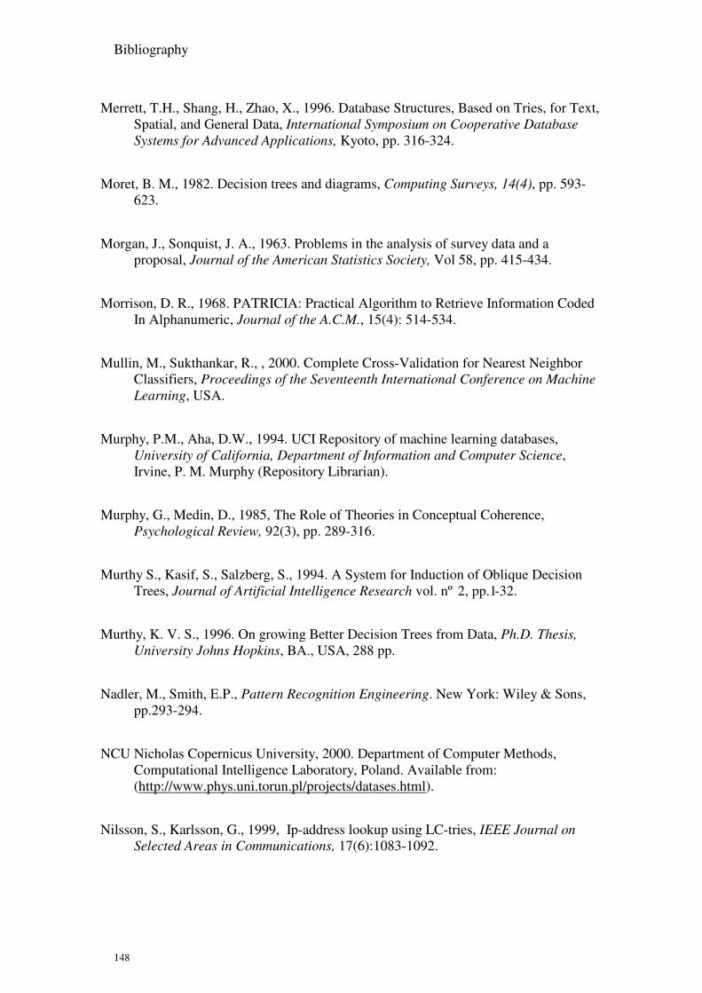
Bibliography
148
Merrett, T.H., Shang, H., Zhao, X., 1996. Database Structures, Based on Tries, for Text, Spatial, and General Data, International Symposium on Cooperative Database Systems for Advanced Applications, Kyoto, pp. 316-324.
Moret, B. M., 1982. Decision trees and diagrams, Computing Surveys, 14(4), pp. 593-623.
Morgan, J., Sonquist, J. A., 1963. Problems in the analysis of survey data and a proposal, Journal of the American Statistics Society, Vol 58, pp. 415-434.
Morrison, D. R., 1968. PATRICIA: Practical Algorithm to Retrieve Information Coded In Alphanumeric, Journal of the A.C.M., 15(4): 514-534.
Mullin, M., Sukthankar, R., , 2000. Complete Cross-Validation for Nearest Neighbor Classifiers, Proceedings of the Seventeenth International Conference on Machine Learning, USA.
Murphy, P.M., Aha, D.W., 1994. UCI Repository of machine learning databases, University of California, Department of Information and Computer Science, Irvine, P. M. Murphy (Repository Librarian).
Murphy, G., Medin, D., 1985, The Role of Theories in Conceptual Coherence, Psychological Review, 92(3), pp. 289-316.
Murthy S., Kasif, S., Salzberg, S., 1994. A System for Induction of Oblique Decision Trees, Journal of Artificial Intelligence Research vol. nº 2, pp.1-32.
Murthy, K. V. S., 1996. On growing Better Decision Trees from Data, Ph.D. Thesis, University Johns Hopkins, BA., USA, 288 pp.
Nadler, M., Smith, E.P., Pattern Recognition Engineering. New York: Wiley & Sons, pp.293-294.
NCU Nicholas Copernicus University, 2000. Department of Computer Methods, Computational Intelligence Laboratory, Poland. Available from: (http://www.phys.uni.torun.pl/projects/datases.html).
Nilsson, S., Karlsson, G., 1999, Ip-address lookup using LC-tries, IEEE Journal on Selected Areas in Communications, 17(6):1083-1092.

Bibliography
149
Ng, A.,Y.,1997. Preventing "overfitting" of cross-validation data. Machine Learning: Proceedings of the Fourteenth International Conference, Nashville, TN, USA, Morgan Kaufmann Publisher, pp. 245-253.
Omachi, S., Aso, H., 2000. A Fast Algorithm for a k-NN Classifier Based on Branch and Bound Method and Computational Quantity Estimation, Systems and Computers in Japan, vol.31, no.6, pp.1-9.
Payne, T., Edwards P., 1998. Implicit Feature Selection with the Value Difference Metric, Proceedings of the 13th European Conference on Artificial Intelligence, ECAI-98, John Wiley & Sons, New York, NY, pp. 450-454.
PMSI, 2002. Software House, Data Mining Tools, France. Available from: http://www.pmsi.fr/
Quinlan, J. R., 1983. Learning efficient classification procedures and their application to chess end games. In R. S. Michalski, J. G. Carbonell, and T. M. Mitchell, editors, Machine Learning, An Artificial Intelligence Approach, Volume I. Morgan Kaufman.
Quinlan, J. R., 1986. Induction of Decision Trees. Machine Learning Journal 1(1):81-106.
Quinlan, J. R., 1988. Bagging, Boosting, and C4.5, University of Sydney.
Quinlan, J. R., 1996. Improved Use of Continuous Attributes in C4.5, Journal of Artificial Intelligence Vol. 4, 77-90.
Quinlan, J.R., 1998. MiniBoosting Decision Trees, Journal of Artificial Intelligence Research.
Riquelme, J., Ferrer, F.J., Aguilar, J., 2001. Búsqueda de un patrón para el valor de k en k-NN, Proceedings of the IX Conferencia de la Asociación Española para la Inteligencia Artificial, Gijón, Spain, Vol. I, pp. 63-72.
Riquelme, J., Aguilar, J. Toro, 2003. M., Finding representative patterns with ordered projections, Pattern Recognition, Vol. 36, pp.1009-1018.
Ripley B.D, 1996. Pattern Recognition and Neural Networks, Cambridge University Press.

Bibliography
150
Risannen, J., 1978, Modelling by shortest data description, Automática Vol 14, pp. 465-471.
Rowland, K.F., 1964. Pattern and Shape, Ginn & Company, Oxford, U.K.
Safavim, S. R., Landgrebe, D., 1991. A survey of decision tree classifier methodology, IEEE Trans. Systems, Man and Cybernetics, vol. 21, pp. 660-674.
Salzberg, S., 1990. Learning with Nested Generalized Exemplars, Norwell, MA: Kluwer Academic Publishers, Boston, MA, USA.
Samet, H., 1984. The quadtree and related hierarquical data structures. Computing Surveys, vol. Nº 16(2), pp.187-260.
Shamir, R., Tsur, D., 1999. Faster Subtree Isomorphism, Journal of Algorithms, Vol. Nº 33, pp.267-280.
Schaffer, C., 1994. Cross-validation, stacking, and bi-level stacking: Meta-methods for classification Learning. In P. Cheeseman & R. W. Oldford Editors, Selecting models from data: Artificial intelligence and statistics IV, New York, Springer-Verlag.
Schapire, R. E., 2002. The boosting approach to machine learning: An overview, In MSRI Workshop on Nonlinear Estimation and Classification.
Serendero, P., Toro, M., 2001. Supervised Learning Using Instance-based Patterns, Proceedings of the IX Conferencia de la Asociación Española para la Inteligencia Artificial, Gijón, Spain, Vol. I, pp. 83-92.
Serendero, P., Toro, M., 2003. Attribute Selection for Classification, Proceedings of the IADIS International Conference, e-Society 2003, Lisbon, Portugal, 3-6 June, A. Palma do Reis, P. Isaías Editors, Vol. I, pp. 469-476.
Skiena, S., Pemmaraju, S., 2002. Computational Discrete Mathematics: Combinatorics and Graph Theory with Mathematica, Cambridge University Press.
Smyth, P., 2001. Data Mining at the interface of computer science and statistics, Chapter 1, in Data Mining for Scientific and Engineering Applications, Grossman, R., Chandrika, K., Kumar, V. Editors, Kluwer Academic Publishers.
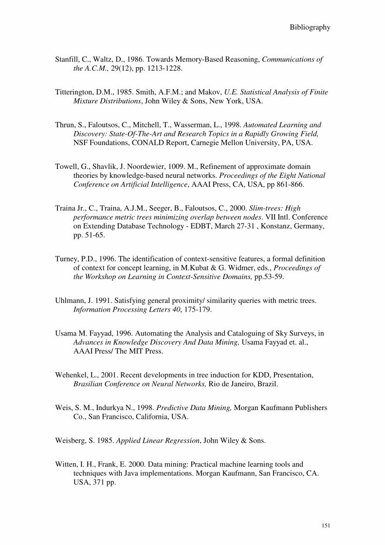
Bibliography
151
Stanfill, C., Waltz, D., 1986. Towards Memory-Based Reasoning, Communications of the A.C.M., 29(12), pp. 1213-1228.
Titterington, D.M., 1985. Smith, A.F.M.; and Makov, U.E. Statistical Analysis of Finite Mixture Distributions, John Wiley & Sons, New York, USA.
Thrun, S., Faloutsos, C., Mitchell, T., Wasserman, L., 1998. Automated Learning and Discovery: State-Of-The-Art and Research Topics in a Rapidly Growing Field, NSF Foundations, CONALD Report, Carnegie Mellon University, PA, USA.
Towell, G., Shavlik, J. Noordewier, 1009. M., Refinement of approximate domain theories by knowledge-based neural networks. Proceedings of the Eight National Conference on Artificial Intelligence, AAAI Press, CA, USA, pp 861-866.
Traina Jr., C., Traina, A.J.M., Seeger, B., Faloutsos, C., 2000. Slim-trees: High performance metric trees minimizing overlap between nodes. VII Intl. Conference on Extending Database Technology - EDBT, March 27-31 , Konstanz, Germany, pp. 51-65.
Turney, P.D., 1996. The identification of context-sensitive features, a formal definition of context for concept learning, in M.Kubat & G. Widmer, eds., Proceedings of the Workshop on Learning in Context-Sensitive Domains, pp.53-59.
Uhlmann, J. 1991. Satisfying general proximity/ similarity queries with metric trees. Information Processing Letters 40, 175-179.
Usama M. Fayyad, 1996. Automating the Analysis and Cataloguing of Sky Surveys, in Advances in Knowledge Discovery And Data Mining, Usama Fayyad et. al., AAAI Press/ The MIT Press.
Wehenkel, L., 2001. Recent developments in tree induction for KDD, Presentation, Brasilian Conference on Neural Networks, Rio de Janeiro, Brazil.
Weis, S. M., Indurkya N., 1998. Predictive Data Mining, Morgan Kaufmann Publishers Co., San Francisco, California, USA.
Weisberg, S. 1985. Applied Linear Regression, John Wiley & Sons.
Witten, I. H., Frank, E. 2000. Data mining: Practical machine learning tools and techniques with Java implementations. Morgan Kaufmann, San Francisco, CA. USA, 371 pp.

Bibliography
152
Wolpert, D.H., 1994. The relationship between PAC, the statistical physics framework, the Bayesian framework and the VC framework, Technical report, The Santa Fe Institute, Santa Fe, N.M., USA.
Wong, A.K.C., Chiu, K.K.Y., 1988. Synthesizing statistical knowledge from incomplete mixed-mode data, IEEE Transactions on Pattern Analysis and Machine Intelligence, TPAMI-9, Nº6, pp. 796-805.
Yianilos, P. N., 1993. Data Structures and Algorithms for Nearest Neighbor Search in General Metric Spaces, Proceedings of ACM-SIAM Symposium on Discrete Algorithms, pp. 311-321.
Zadrozsny, B., 2001. Reducing Multiclass to binary by coupling probability estimates, To appear in Advances in Neural Information Processing Systems 14 (NIPS*2001), Canada.
Zadrozsny, B., Elkan, C., 2002. Transforming Classifying Scores into Accurate Multiclass Probabilities Estimates, To appear, Proceedings of the Eighth International Conference on Knowledge Discovery and Data Mining (KDD'02).
Zhou, Z. H., 2003. Three perspectives of data mining. Artificial Intelligence, Nº 143(1), pp. 139-146.�
Zhu, S., Li, T., Ogihara, M., 2002. CoFD: An Algorithm for Non-distance Based Clustering in High Dimensional Spaces, 4thInternational Conference on Data Warehousing and Knowledge Discovery, Aix en Provence, France.

153
Appendix I. Example of Dictionary corresponding to the Annealing
Dataset
Each line contains the following elements: Number, description, Type, initial value, end value, interval size, class flag, #,symbolic values. Allowable types: N=discrete, R=continuous, D=symbolic known values, S= symbolic
unknown values, C=Class -------------------------------------------------------------------------------------------------------
1, hardness, N, 0, 85, 1, N
2, width, R, 0, 1525, 20, N
3, surface-quality, D, 0, 6, 1, N,#,-,D,E,F,G,
4, carbon, N, 0, 70, 1, N
5, steel, D, 0, 10, 1, N,#,-,R,A,U,K,M,S,W,V,
6, family, D, 0, 11, 1, N,#,-,GB,GK,GS,TN,ZA,ZF,ZH,ZM,ZS,
7, strength, N, 0, 700, 10, N
8, chrom, D, 0, 3, 1 ,N,#,C,-,
9, oil, D, 0, 4, 1, N,#,-,Y,N,
10, ferro, D, 0, 3, 1, N,#,Y,-,
11, len, R, 0, 4880, 40, N
12, enamelability, D, 0, 7, 1, N,#,-,1,2,3,4,5,
13, surface-finish, D, 0, 4, 1, N,#,P,M,-,
14, formability, D, 0, 7, 1, N,#,-,1,2,3,4,5,
15, packing, D, 0, 5, 1, N,#,-,1,2,3,
16, phos, D, 0, 3, 1, N,#,P,-,
17, exptl, D, 0, 3, 1, N,#,Y,-,
18, BlueBrightVarnClean, D, 0, 6, 1, N,#,B,R,V,C,-,
19, product-type, D, 0, 4, 1, N,#,C,H,G,
20, temper_rolling, D, 0, 3, 1, N,#,-,T,
21, condition, D, 0, 5, 1, N,#,-,S,A,X,
22, non-ageing, D, 0, 3, 1, N,#,-,N,
23, bc, D, 0, 3, 1, N,#,Y,-,
24, bf, D, 0, 3, 1, N,#,Y,-,
25, bt, D, 0, 3, 1, N,#,Y,-,
26, bw/me, D, 0, 4, 1, N,#,B,M,-,
27, bl, D, 0, 3, 1, N,#,Y,-,
28, m, D, 0, 3, 1, N,#,Y,-,
29, cbond, D, 0, 3, 1, N,#,Y,-,

154
30, marvi, D, 0, 3, 1, N,#,Y,-,
31, corr, D, 0, 3, 1, N,#,Y,-,
32, lustre, D, 0, 3, 1, N,#,Y,-,
33, jurofm, D, 0, 3, 1, N,#,Y,-,
34, s, D, 0, 3, 1, N,#,Y,-,
35, p, D, 0, 3, 1, N,#,Y,-,
36, shape, D, 0, 3, 1, N,#,COIL,SHEET,
37, thick, R, 0, 4000, 40, N
38, bore, D, 0, 5, 1, N,#,0000,0500,0600,0760,
39, classes, C, 0, 5, 0, S

155
Appendix II. Settings for the execution of the Naive Bayes classifier

156
Parameter values settings for the execution of the J48 (C4.5) classifier.

Bibliography
157
Parameter values settings for the execution of the IBk (k-NN) classifier.

158

Bibliography
159
Appendix III. Alpha values for Decision Parameters
Table A-1 Weights (alpha) for various ambit and precision values expressed in percentage
ambit precision alpha ambit precision alpha 10 10 53 50 60 282 10 20 72 50 70 301 10 30 91 50 80 320 10 40 111 50 90 339 10 50 131 50 100 359 10 60 151 60 10 233 10 70 171 60 20 247 10 80 191 60 30 263 10 90 211 60 40 281 10 100 230 60 50 298 20 10 88 60 60 316 20 20 106 60 70 335 20 30 124 60 80 354 20 40 144 60 90 373 20 50 163 60 100 392 20 60 183 70 10 269 20 70 202 70 20 283 20 80 222 70 30 299 20 90 242 70 40 316 20 100 262 70 50 333 30 10 124 70 60 351 30 20 141 70 70 369 30 30 158 70 80 388 30 40 177 70 90 406 30 50 196 70 100 425 30 60 215 80 10 306 30 70 235 80 20 320 30 80 254 80 30 335 30 90 274 80 40 351 30 100 294 80 50 368 40 10 160 80 60 386 40 20 176 80 70 403 40 30 193 80 80 422 40 40 211 80 90 440 40 50 230 80 100 459 40 60 249 90 10 342 40 70 268 90 20 356

160
40 80 287 90 30 371 40 90 306 90 40 387 40 100 326 90 50 403 50 10 196 90 60 421 50 20 211 90 70 438 50 30 228 90 80 456 50 40 246 90 90 474 50 50 264 90 100 493