Embed Size (px)
Citation preview
AGH University of Science and Technology Faculty of Mechanical Engineering and Robotics
Doctoral Thesis
Welding sequence Analysis By
Isaac Hernández Arriaga
Co‐Advisor: Dr. Hab. Piotr Rusek, Prof. AGH Dr. Eduardo Aguilera Gómez
September 2009
Welding Sequence Analysis
i Isaac Hernández Arriaga
ABSTRACT
This thesis has been divided in nine chapters. Chapter 1 provides brief background and general and specific objectives of this work. Chapter 2 presents the methods and advantages of reducing or controlling residual stresses and distortion induced by the welding process as well as a definition and classification of the welding sequence. It also presents a study of the welding sequence analysis, a survey of previous research in the field of welding sequences, and a discussion of its advantages, disadvantages, scope, and limitations. The subject of Chapter 3 is the finite element modeling of the welding processes, defining the boundary and initial conditions of the welding process and studying the effects of the welding sequence on the residual stress distribution and distortion in symmetrical structures. It should be noted that the proposed numerical model has general applicability and is not limited to symmetrical structures. The proposed sequentially-coupled thermo-mechanical analysis involves two steps. A transient heat transfer analysis is performed followed by a thermal elastic plastic analysis. This numerical simulation is performed in an I-type specimen subject to tension and validated with experimental data [25]. Finally, the chapter presents a numerical simulation of the welding sequence in an L-type structure to demonstrate that the proposed numerical model accurately simulates the effects of the welding sequence on residual stresses and distortion. Chapter 4 presents a study of the effects of the welding sequence on residual stresses and distortion in a stiffened symmetrical flat frame. Selected welding sequences reduce residual stresses, distortion, or the relation between both parameters. These proper welding sequences are obtained from empirical welding rules, axis of symmetry, center of gravity of the frame, and concentric circles. The origin of the circles coincides with the center of gravity of the frame, and the radius of the circles is formed by the center of gravity of the frame with the center of gravity of each of the weld beads. The different welding sequences are analyzed with the numerical model developed in chapter 3. Finally, the chapter presents a procedure to determine the proper welding sequences to reduce residual stress, distortion or the relation between both parameters for 2-dimensional symmetrical structures. The main goal chapter 5 is to demonstrate that the procedure to determine the proper welding sequences to reduce residual stress, distortion or the relation between both parameters in 2-dimensional symmetrical structures can be applied to 3-dimensional symmetrical structures. This is done by studying the effects of the

Welding Sequence Analysis
ii Isaac Hernández Arriaga
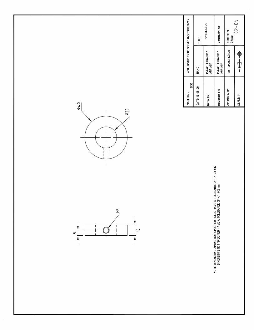
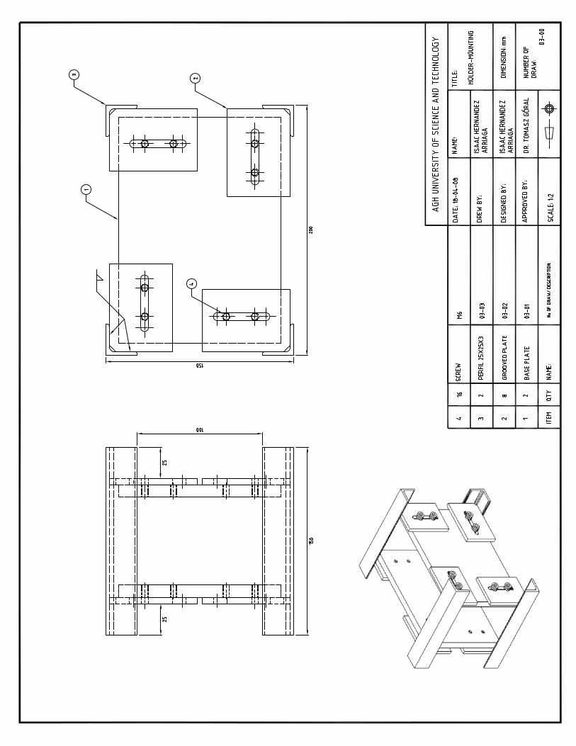
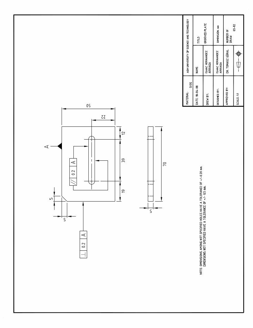
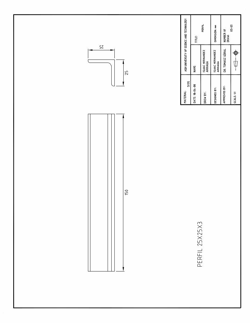
welding sequence on the residual stresses and distortion in a 3-dimensional unitary cell-type symmetrical structure. Now the weld bead circles become spheres. To demonstrate the procedure to determine the proper welding sequence for 3-dimensional symmetrical structures, four numerical simulations are performed in the proposed symmetrical structure. Two of these numerical simulations deal with the proper welding sequence to reduce residual stress and the other two deals with the proper welding sequence to reduce distortion. Also, the numerical simulation of a special welding sequence is performed for comparison with the proper welding sequence to reduce distortion. This special welding sequence applies the external weld beads first and the internal weld beads later. All the numerical simulations are based on the proposed numerical model of the welding process developed in Chapter 3. Chapter 6 presents a methodology for the development of the experimental tests. This methodology helps to plan, execute, and control each of the stages of the experimental tests. The methodology starts with the material selection of the specimen, configuration selection, welding process selection, metal transfer mode selection, welding parameter selection, design and fabrication of the equipment needed to run the test, design and fabrication of the mounting locks, residual stresses relief caused by the manufacturing process, transportation, handling, storage and cutting of the plates, measurement of the initial distortion of the plates, design and fabrication of a holder-mounting device to hold the plates, design and fabrication of a square-mounting device to square the holder-mounting device, application of welding tacks, measurement of the distortion after applying the welding tacks, installation of the run-off tabs, application of the welding, removal of the run-off tabs of the welded structure, measurement of the distortion after welding, and measurement of the final distortion induced by the welding process. Chapter 7 covers the results of the experimental tests performed in 3-dimensional unitary cell-type symmetrical specimens. In these experimental tests, the effects of the welding sequence on distortion are studied. Eight symmetrical specimens are prepared. Four welding sequences are considered: two of them are adequate to reduce distortion and the other two reduce residual stresses. The chapter also studies the effects that occur when a welding bead is divided into 3 sub-weld beads, as well as the effects of relieving the residual stresses caused by manufacturing process, transportation, storage and cutting of plates. Welding tacks are applied to all specimens before the actual weld process begins. The measurement of the distortion is periodically performed to observe if rheological effects occur in the specimens after welding. The experimental tests were performed in the Department of Machine Strength and Manufacturing in the Faculty of Mechanical Engineering at the University of Science and Technology in Krakow, Poland. Chapter 8 presents a comparison between the numerical results obtained in Chapter 5 and the experimental results obtained in Chapter 7 for the 3-dimensional unitary cell-type symmetrical structure. The comparison discusses the distortion modes and the distortion in the 24 points of interest. The chapter presents the procedures to determine the proper welding sequences to reduce the residual stresses, distortion, or a relation between both parameters in symmetrical and asymmetrical structures in 2 and 3
Welding Sequence Analysis
iii Isaac Hernández Arriaga
dimensions. These procedures were developed in chapters 4 and 5 to determine the proper welding sequences to reduce residual stresses, distortion, or relation between both parameters in symmetrical structures in 2 and 3 dimensions. Chapter 9 presents the conclusions, contributions and suggestions for future work.

Welding Sequence Analysis
iv Isaac Hernández Arriaga
ACKNOWLEDGMENTS
I am extremely grateful for the support of the University of Guanajuato and AGH University of Science and Technology. They provide employment and resources which made it possible for me to pursue this degree. I wish to express my sincere appreciation to Dr. Eduardo Aguilera for his guidance, encouragement and insight throughout the duration of this research. I would also express my gratitude to Professor Piotr Rusek for his encouragement and support, his influence extends far beyond my academic work. I wish to tanks to Dr. Arturo Lara, Dr. Elias Ledesma, Professor Stanisław Wolny, and Professor Andrzej Skorupa for serving as dissertation committee members and providing positive suggestion and comments. I acknowledge the Consejo Nacional de Ciencia y Tecnología (CONACYT), Dirección de Relaciones Academicas Internacionales e Interinstitucionales (DRAII), and Dirección de Investigación y Posgrado (DINPO) of the University of Guanajuato for the funding of doctoral studies, doctoral research and stay at AGH.
I would also like to express my gratitude to Director of the engineering division of the Irapuato-Salamanca Campus; Dr. Oscar Ibarra, for his invaluable support in the completion of my doctoral studies.
I would especially like to thank the Authorities of the AGH University of Science and Technology; Rector, Professor Antoni Tajduś, Vice-Rector for Cooperation and Development, Professor Jerzy Lis, and Dean of the faculty of Mechanical Engineering and Robotics, Professor Janusz Kowal for thier invaluable collaboration with the University of Guanajuato.
I am also grateful to Dr. Hector Plascencia for his interest and help to my research. Also, I would like to thank to Dr. Pedro de Jesús García and to Dr. Rogelio Navarro for their initial help, interest and advice. I am very grateful to Dr. Tomasz Góral for his help on experimental research. Thanks are also extended to Drs. Jerzy Haduch and Andrzej Tyka for their assistance.

Welding Sequence Analysis
v Isaac Hernández Arriaga
During my stay at AGH, I was fortunate to have had a number of talented technical workers. Kazimierz Nawrot, Włodzimierz Rusek, and Artur Konopczak all helped with the fabrication of the equipment needed to run the test. My thanks to Salvador Martínez, for his friendly help in the experimental measurements at AGH. The same quality of special thanks goes to Mr. Guadalupe Negrete for his expertise and generous help in welding . My special thanks go to Renato Sánchez for giving me their generous and solidary support. To all my friends and classmates, especilly Hijinio Juárez, Alejandro León, Sergio Pacheco and Mr. Baldomero Lucero, thank you for your warm friendships. To Ms. Ma. Eugenia Gallardo, secretary of our Mechanical Department, for helping me during my studies. My academic achievements would have been impossible without the spiritual support of my family. Special thanks are due to my parents, Beny Arriaga and Daniel Hernández. Their sacrifice for my education made me who I am. Thanks are also extended to my sister and brother; Ruth Hernández and Daniel Hernández, for their understanding and support for my studies. Special love goes to my wife, Maria Victoria Cabrera whose boundless love and encouragement made my time at University of Guanajuato and AGH easy and pleasant. Also, my cute son, Samuel Isaac Hernández, enabled me to periodically escape the academic pressure with his smiles. Finally, I thank an anonymous editor for assisting with the English version of my thesis.

Welding Sequence Analysis
vi Isaac Hernández Arriaga
TABLE OF CONTENTS Abstract i Acknowledgments iv Table of contents vi List of figures xii List of tables xvii Nomenclature xix Chapter I INTRODUCTION
1.1 Background 1 1.2 General objective 2 1.3 Specific objectives 2
Chapter II WELDING SEQUENCE BACKGROUND AND METHODS FOR CONTROLLING RESIDUAL STRESSES AND DISTORTION INDUCED BY WELDING
2.1 Introduction 3 2.2 Advantages of residual stress and distortion control 3 2.3 Methods to control welding-induced residual stress and distortion 4
2.3.1 Welding sequence 4 2.3.2 Definition of weld parameter 4 2.3.3 Weld procedure 5 2.3.4 Fixture design 5 2.3.5 Precambering 5 2.3.6 Prebending 6 2.3.7 Thermal tensioning 6 2.3.8 Heat sink welding 7 2.3.9 Preheating 7 2.10 Post-weld heat treatment 7 2.11 Post-weld corrective methods 7
2.4 Welding sequence definition 8 2.5 Welding sequence classification 8
2.5.1 Welding sequence for single pass welds 8 2.5.2 Welding sequence for multiple pass welds 9

Welding Sequence Analysis
vii Isaac Hernández Arriaga
2.6 Welding sequence selection based on empiric rules 10 2.7 Welding sequence background 11 2.8 Summary of the welding sequence analysis background 43 2.9 Matrix of the welding sequence analysis background 44
Chapter III PROPOSAL OF A NUMERICAL SIMULATION OF THE WELDING PROCESS AND A NUMERICAL SIMULATION OF THE WELDING SEQUENCE IN AN L-TYPE STRUCTURE
3.1 Introduction 45 3.2 Heat transfer in welding 45
3.2.1 Analytical solution for the temperature field 46 3.2.2 Thermal Initial and boundary Conditions 48
3.3 Thermal elastic plastic stress analysis in welding 50 3.3.1 Mechanical equations 50 3.3.2 Mechanical initial and boundary conditions 51
3.4 Finite element solution of the welding 51 3.4.1 Finite element solution of heat transfer in welding 51 3.4.2 Finite element solution of the thermal elastic plastic stress analysis in welding 52
3.5 Geometric configuration of I-type specimen subject to tension 55 3.6 Material selection for the I-type specimen subject to tension 56 3.7 Temperature-dependent thermal and mechanical properties of ASTM A36 56 3.8 Finite element model of the I-type specimen subject to tension 57
3.8.1 Definition and justification of the applied finite elements 58 3.8.2 Thermal initial and boundary conditions 61 3.8.3 Mechanical boundary condition 61 3.8.4 Body load 61 3.8.5. Solution of the finite element model 62
3.9 Points of interest in the finite element model of the I-type specimen subject to tension 62 3.10 Residual stresses in the I-type specimen subject to tension obtained in the numerical simulation 62 3.11 Comparison between the numerical and experimental results of an I-type specimen subject to
tension 63
3.12 Conclusions of the numerical simulation of the welding process in an I-type specimen subject to tension
64
3.13 Numerical simulation of the welding sequence in an L-type structure 65 3.14 Geometric configuration of the L-type structure 65 3.15 Finite element model of the L-type structure 65 3.15.1 Thermal initial and boundary conditions 66 3.15.2 Mechanical boundary conditions 67
Welding Sequence Analysis
viii Isaac Hernández Arriaga
3.15.3 Solution of the finite element model of the L-type structure 67 3.16 Configuration of welding sequences for the L-type structure 67 3.17 Localization of the point of interest in the L-type structure 68 3.18 Numerical results in the L-type structure 68 3.18.1 Distortion profile in the L-type structure 70 3.18.2 Residual stress distribution in the L-type structure 70 3.19 Experimental tests for the L-type structure 71 3.19.1 Selection of points of interest in the L-type structure 72 3.19.2 Configuration of the welding sequences in the L-type specimens 72 3.19.3 Measurement of distortion on L-type specimens 73 3.20 Conclusions of the welding sequence analysis of the L-type structure 75 Chapter IV WELDING SEQUENCE ANALYSIS IN A STIFFENED SYMMETRICAL 2-DIMENSIONAL FRAME
4.1 Introduction 76 4.2 Geometric configuration of a stiffened symmetrical flat frame 76 4.3 Welding configuration in the stiffened symmetrical flat frame 77 4.4 Finite element model of the stiffened symmetrical flat frame 80
4.4.1 Thermal initial and boundary conditions 81 4.4.2 Mechanical boundary conditions 81 4.4.3 Solution of the finite element model of the stiffened symmetrical flat frame 82
4.5 Numerical results in the stiffened symmetrical flat frame 82 4.5.1 Distribution of the residual stresses in the stiffened symmetrical flat frame 82 4.5.2 Distortion profile in the stiffened symmetrical flat frame 83
4.6 Analysis of residual stress-distortion relations analysis 83 4.7 Order of importance of the welding sequences to reduce residual stress, distortion, or the
relation between them in the stiffened symmetrical flat frame 84
4.8 Proper welding sequences to reduce the residual stress, distortion, or a relation between them in the stiffened symmetrical flat frame
84
4.8.1 Proper welding sequence to reduce the residual stress in the stiffened symmetrical flat frame
86
4.8.2 Proper welding sequence to reduce distortion in the stiffened symmetrical flat frame 87 4.8.3 Proper welding sequence to improve the relation between both critical parameters in the
stiffened symmetrical flat frame 87
4.9 Hypothesis to determine the proper welding sequence to reduce the residual stress, distortion, or a relation between them in symmetrical flat structures
88
4.10 Experimental tests in a stiffened symmetrical flat frame specimen 89 4.10.1 Selection of points of interest in the stiffened symmetrical flat specimen 90

Welding Sequence Analysis
ix Isaac Hernández Arriaga
4.10.2 Configuration of the welding sequence in the stiffened symmetrical flat specimen 90 4.10.3 Measurement of distortion on the stiffened symmetrical flat specimen 91
4.11 Conclusions of the welding sequence analysis of stiffened symmetrical flat frame 93 Chapter V WELDING SEQUENCE ANALYSIS IN A 3-DIMENSIONAL UNITARY CELL-TYPE SYMMETRICAL STRUCTURE
5.1 Introduction 95 5.2 Hypothesis to determine the proper welding sequence to reduce the residual stress, distortion,
or a relation between them in 3-dimensional symmetrical structures 96
5.3 Geometric configuration of the 3-dimensional unitary cell 97 5.4 Selection of the number of weld beads in the 3-dimensional unitary cell 98 5.5 Symmetry axis selection and formation of the concentric spheres in the 3-dimensional unitary
cell 98
5.6 Proper welding sequence to reduce the residual stress and proper welding sequence to reduce the distortion in the 3-dimensional unitary cell
100
5.7 Material selection of the 3-dimensional unitary cell 101 5.8 Fillet weld shape used in the 3-dimensional unitary cell 101 5.9 Finite element model of the 3-dimensional unitary cell 101
5.9.1 Thermal initial and boundary conditions 102 5.9.2 Mechanical boundary conditions 103 5.9.3 Solution of the finite element model of the 3-dimensional unitary cell 103
5.10 Localization of the points of interest in the 3-dimensional unitary cell 103 5.11 Configuration of the numerical simulation for the 3-dimensional unitary cell 104 5.12 Numerical results of the different welding sequences analyzed in the 3-dimensional unitary cell 105
5.12.1 Maximum von Mises residual stress in the 3-dimensional unitary cell 105 5.12.2 Distortion modes in the 3-dimensional unitary cell 106 5.12.3 Maximum distortion and distortion in 24 points of interest in the 3-dimensional unitary
cell 106
5.13 Numerical comparison between the proper welding sequence to reduce distortion and a special welding sequence in the 3-dimensional unitary cell
107
5.14 Conclusions of the welding sequence analysis of the 3-dimensional unitary cell 109 Chapter VI METHODOLOGY OF EXPERIMENTAL TESTS
6.1 Introduction 110 6.2 Specimen material selection 110 6.3 Selection of specimen configuration 111 6.4 Selection of the welding process 111
Welding Sequence Analysis
x Isaac Hernández Arriaga
6.5 Selection of metal transfer mode 111 6.6 Selection of welding parameters (Operating variables) 112
6.6.1 Arc voltage and welding current 112 6.6.2 Welding speed 113 6.6.3 Wire feed rate 113 6.6.4 Selecting of contact tip to work distance 114 6.6.5 Electrode orientation 114 6.6.6 Electrode diameter 115 6.6.7 Shielding gas composition 115 6.6.8 Gas flow rate 116
6.7 Design and fabrication of the equipment needed to run the test 116 6.8 Design and fabrication of the mounting locks 117 6.9 Relief of residual stresses caused by the manufacturing process, transportation, handling,
storage and cutting of the plates 118
6.10 Measurement of the initial plate distortion 119 6.11 Design and fabrication of a holder-mounting device to hold the plates 120 6.12 Design and fabrication of a square-mounting device 120 6.13 Application of the welding tacks 121 6.14 Distortion measurement after welding tack application 123 6.15 Installation of the run-off tabs 123 6.16 Application of the welding 124 6.17 Removing the run-off tabs from the welded structure 124 6.18 Measurement of the distortion after applying the welding 125 6.19 Measurement of the final distortion 126 Chapter VII RESULTS OF THE EXPERIMENTAL TESTS IN 3-DIMENSIONAL UNITARY CELL-TYPE SPECIMENS 7.1 Introduction 127 7.2 Configuration of the 3-dimensional unitary cell specimens 127 7.3 Localization of the points of interest in the 3-dimensional unitary cell specimens 128 7.4 Configuration of the experiment 128 7.5 Distortion after applying welding tacks in the 3-dimensional unitary cell specimens 128 7.6 Distortion after welding in the 3-dimensional unitary cell specimens 129 7.7 Distortion modes of the 3-dimensional unitary specimens 132 7.8 Final distortion of the 3-dimensional unitary cell specimens 133 7.9 Final Remarks for distortion of the 3-dimensional unitary cell specimens 135 7.10 Conclusions of the results of the experimental test in 3-dimensional unitary cell specimens 136

Welding Sequence Analysis
xi Isaac Hernández Arriaga
Chapter VIII COMPARISON BETWEEN THE “3- DIMENSIONAL UNITARY CELL”-TYPE STRUCTURES/SPECIMENS 8.1 Introduction 137 8.2 Comparison of distortion modes 137 8.3 Comparison of distortion 137 8.4 Conclusions of the comparison between numerical and experimental results 140 8.5 Procedures to determine the proper welding sequences to reduce residual stress, distortion, or
a relation between them in symmetrical and asymmetrical structures in 2 and 3 dimensions 140
8.5.1 Symmetrical structures in 2 and 3 dimensions 140 8.5.2 Asymmetrical structures in 2 and 3 dimensions 142 Chapter IX CONCLUSIONS, CONTRIBUTIONS, AND SUGGESTIONS FOR FUTURE RESEARCH 9.1 Conclusions 146 9.2 Contributions 147 9.3 Suggestion for future research 147 REFERENCES 149 APPENDIX
1 Plasticity theory applied to welding process and its formulation by finite element method 151 2 Definition and justification of the applied finite elements 171 3 Response to critical comments 179 4 Proper welding sequence to reduce residual stress and distortion in common symmetrical
structures in 2 and 3 dimensions based on the hypothesis developed in the sections 4.9 and 5.2. 188
5 Listing of commands of the numerical simulation of the welding process (I-type specimen subject to tension)
191
6 Listing of commands of the numerical simulation of the welding sequence in an L-type structure (Welding sequence No.1)
194
7 Listing of the commands of the numerical simulation of stiffened symmetrical flat frame (welding sequence No.5 with welding tacks)
197
8 Listing of the commands of the numerical simulation of the 3-dimensional unitary cell-type symmetrical structure (welding sequence most appropriate to reduce distortion with 24 weld beads and welding tacks)
201
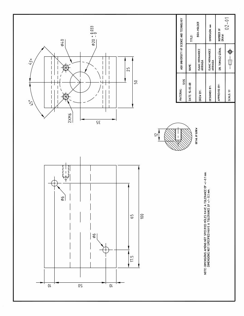
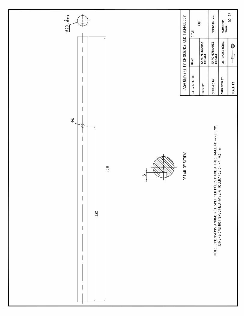
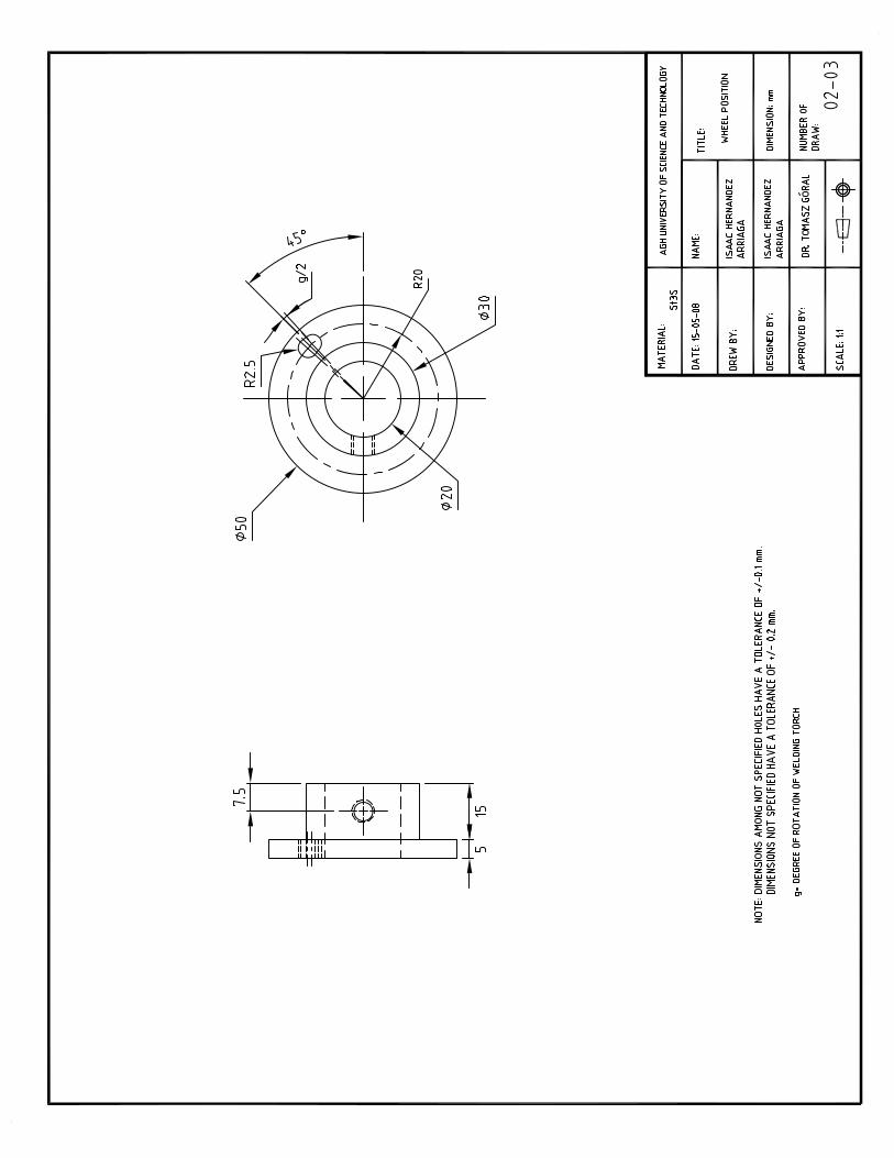
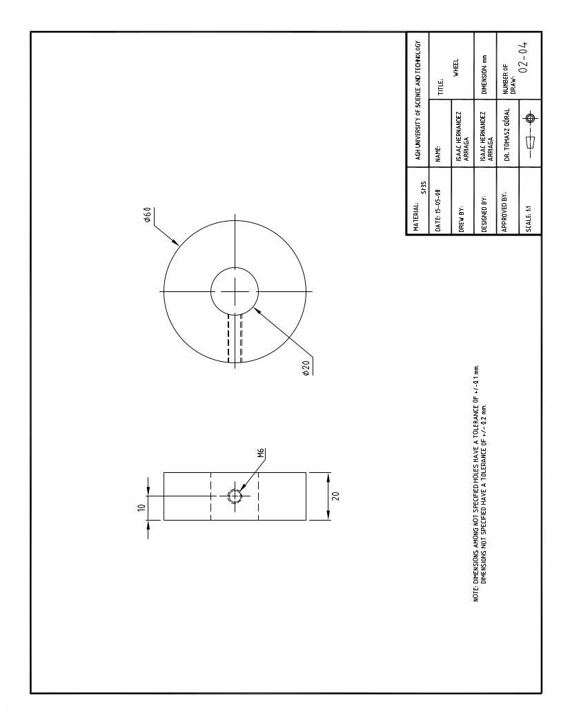
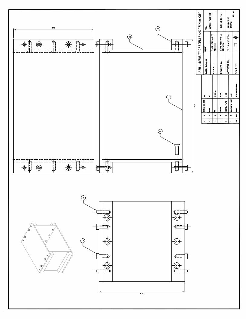
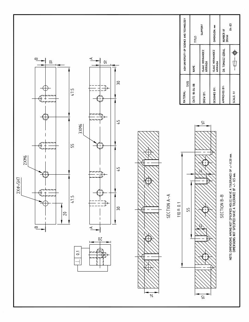
9 Construction drawings 205
Welding Sequence Analysis
xii Isaac Hernández Arriaga
LIST OF FIGURES
CHAPTER II
Figure 2.1 Welded frame distortion [4]: (a) Without considering a proper welding sequence, (b) considering a proper welding sequence
4
Figure 2.2 Rigid supports [4] 5 Figure 2.3 Precamber with a curved surface [2] 6 Figure 2.4 Pre-bending [2] 6 Figure 2.5 Welding with the thermal tensioning process [11] 6 Figure 2.6 Heat sink welding [1] 7 Figure 2.7 Sequences for thin-wall butt-welds [3]: (a) Progressive, (b) backstep, (c) symmetric, and
(d) jump 8
Figure 2.8 Built-Up welding sequence on thick-wall butt-weld [3] 9 Figure 2.9 Block welding sequence [3] 9 Figure 2.10 Cascade welding sequence [3] 9 Figure 2.11 Welding sequences for thin-wall butt-welds [16]: (a) Progressive, (b) backstep, and (c)
symmetric 11
Figure 2.12 Longitudinal residual stress distribution [16]: (a) Along the X-direction and (b) along the Y-direction
12
Figure 2.13 Different welding sequence for thick-wall butt-welds [16] 13 Figure 2.14 Residual stresses distribution along the X-direction in various welding sequence for
thick-wall butt-welds [16]: (a) Longitudinal and (b) transverse 14
Figure 2.15 Geometry and various welding sequence for circular patch [16]: (a) Geometry of circular patch welding, (b) Progressive sequence, (c) backstep sequence, and (d) jump sequence
15
Figure 2.16 Residual stresses distribution for various welding sequence [16]:(a) Circumferential and (b) radial
16
Figure 2.17 Dimensions of the specimen, mm. [17] 17 Figure 2.18 Schematic of Weld bead´s delamination [17] 17 Figure 2.19 Comparison of transverse residual stress between in the same direction and welding in
the inverse direction [17] 18
Figure 2.20 Configuration of welded blocks in a multi-block welding sequence [18] 19 Figure 2.21 Structural boundary conditions of welded plates (clamp fixture at both sides) [18] 19 Figure 2.22 Resulted distortion profile for two different block sequences [18]: (a) Welding sequence
No. 1 and (b) welding sequence No. 2 20
Welding Sequence Analysis
xiii Isaac Hernández Arriaga
Figure 2.23 Resulted distribution of the Von Mises stress using different block sequences. [18]: (a) Welding sequence No. 1 and (b) welding sequence No. 2
21
Figure 2.24 Configuration of a large-diameter multi-pass pass butt-welded pipe joints and its cross section [19]
22
Figure 2.25 Welding sequences for a multi-pass Welded pipe joint [19] 22 Figure 2.26 Comparison of circumferential residual stress in multi-pass welded pipe joints [19]: (a)
Inner surface and (b) outer surface 23
Figure 2.27 Comparison of axial residual stress in multi-pass welded pipe joints [19]: (a) Inner surface and (b) outer surface
24
Figure 2.28 Comparison of residual stress across through-thickness along the heat-affected zone in multi-pass welded pipe joints [19]: (a) Circumferential and (b) axial
25
Figure 2.29 Configuration of a multi-pass fillet Weld joint, mm. [20] 27 Figure 2.30 Different welding sequences in multi-pass fillet weld joint [20] 27 Figure 2.31 Comparison of residual stress in a multi-pass fillet weld joint [20]: (a) Case 1 and
(b) case 2 28
Figure 2.32 Relation between nominal stress range and fatigue life in multi-pass fillet weld joints [20]
29
Figure 2.33 Aluminum panel for study on welding sequence effect on angular distortion [21] 30 Figure 2.34 Welding sequences for angular distortion analysis of aluminum panel structure[21] 31 Figure 2.35 Distortion displacements at four cross sections of the panel from four welding
sequences [21]: (a) At x= 16 inch; (b) at x=32 inch; (c) at y= 9.3 inch; y (d) at y=30 inch. 32
Figure 2.36 Optimum welding sequence determined by JRM [21] 33 Figure 2.37 Comparison of distortion resulting from welding sequence and the optimum welding
sequence [21]: (a) at x= 16 inch, (b) at x=32 inch, (c) at y= 9.3 inch, and (d) at y=30 inch. 33
Figure 2.38 T-joint configuration [22]: (a) Finite element model and (b) dimensions of the cross section of the hollow extrusions
34
Figure 2.39 Different welding sequences [22]: (a) Case 1 and (b) case 2 34 Figure 2.40 Comparison of measured (M) and calculated (S) distortion evolution for two welding
sequence [22]: (a) Case 1 and (b) case 2 35
Figure 2.41 Geometric configuration of a sub-assembly [15] 36 Figure 2.42 Simplified model with torsion springs [15] 36 Figure 2.43 Final exaggerated deformed shapes for different sequences [15] 37 Figure 2.44 Geometric configuration and dimensions of weldment [23] 38 Figure 2.45 Code to designate the welding sequence and welding direction [23] 39 Figure 2.46 Radial displacement of the edge of plate with respect to θ for continuous welding and
the optimum sequence[23] 39
Figure 2.47 Tail bearing housing [24] 41 Figure 2.48 Finite element model of welding process and designation of welding paths showing 41

Welding Sequence Analysis
xiv Isaac Hernández Arriaga
positive orientation of weld and reference number in sequence [24] Figure 2.49 Run 28 is the optimized displacement with a clamped structure [24] 42 Figure 2.50 The absolute values of the X displacement for all 28 sequences [24] 42 CHAPTER III
Figure 3.1 Eulerian frame and thermal initial and boundary conditions 49 Figure 3.2 Geometric configuration of I-type specimen subject to tension (mm) [25] 55 Figure 3.3 Thermal and mechanical properties of ASTM A36 as a function of temperature [34] 56 Figure 3.4 Stress-strain behavior of ASTM A36 carbon steel for different temperatures [Based in
figure 3.3] 57
Figure 3.5 Finite element mesh of the I-type specimen subject to tension 58 Figure 3.6 Weld thermal cycle of ASTM A36 carbon steel [34-35] 60 Figure 3.7 Localization of the points of interest on finite element model 62 Figure 3.8 Distribution of residual stresses in the X-direction in the I-type specimen subject to
tension 63
Figure 3.9 Experimental tests: a) Localization of the points of interest in the I-type specimen subject to tension, mm. b) welding parameters employed [25]
64
Figure 3.10 Geometric configuration of the L-type structure (mm) 65 Figure 3.11 Finite element model of the L-type structure 66 Figure 3.12 Localization of the node 1533 in the L-type structure 68 Figure 3.13 Maximum distortions in L-type structure for three different welding sequences 69 Figure 3.14 Maximum Von Mises residual stress in the L-type structure for three different welding
sequences 69
Figure 3.15 Distortion profile in the L-type structure corresponding to welding sequence 3 70 Figure 3.16 Distribution of Von Mises residual stress corresponding to the welding sequence 2 71 Figure 3.17 Localization of the interest points in the L-type specimen 72 Figure 3.18 L-type specimen 2 after applying the welding sequence 3 73 Figure 3.19 L-type specimen 2 (welding sequence 3) mounted on the coordinate measuring
machine 73
Figure 3.20 Comparison of the welding distortion (exaggerated) between two L-type specimens 75 CHAPTER IV Figure 4.1 Geometric configuration of the stiffened symmetrical flat frame (mm) 77 Figure 4.2 Finite element model of the stiffened symmetrical flat frame 80 Figure 4.3 Distribution of Von Mises residual stresses corresponding to the welding sequence
(5 I-O) 82

Welding Sequence Analysis
xv Isaac Hernández Arriaga
Figure 4.4 Distortion profile corresponding to the welding sequence 5 O-I WT 83 Figure 4.5 Centers of gravity of the structure, centers of gravity of the weld beads, axis of
symmetry and concentric circles in the stiffened symmetrical flat frame 86
Figure 4.6 Ranges of the values of P and W for welding sequence 1 I-O and combined welding sequence
87
Figure 4.7 Localization of the point of interest in the stiffened symmetrical flat specimen 90 Figure 4.8 Stiffened symmetrical flat specimen after applying the welding sequence 5 O-I WT 91 Figure 4.9 Stiffened symmetrical flat specimen mounted on the coordinate measuring machine 91 Figure 4.10 Distortion profile in the stiffened symmetrical flat specimen corresponding to welding
sequence 5 O-I WT (exaggerated) 93
CHAPTER V
Figure 5.1 Panel used in the welding industry 97 Figure 5.2 Configurations and dimensions of the 3-dimensional unitary cell (mm) 98 Figure 5.3 Axis of symmetry and concentric spheres of the 3-dimensional unitary cell formed by 24
fillet welds 99
Figure 5.4 Different welding sequences for the 3-dimensional unitary cell 100 Figure 5.5 Fillet weld shape used in the 3-dimensional unitary cell 101 Figure 5.6 Finite element model of the 3-dimensional unitary cell 102 Figure 5.7 Localization of the points of interest in the 3-dimensional unitary cell 104 Figure 5.8 Distribution of residual stresses corresponding to numerical simulation 2 105 Figure 5.9 Isometric view of the distortion profile corresponding to the numerical simulation 3 106 Figure 5.10 Configuration of the special welding sequence 108
CHAPTER VI
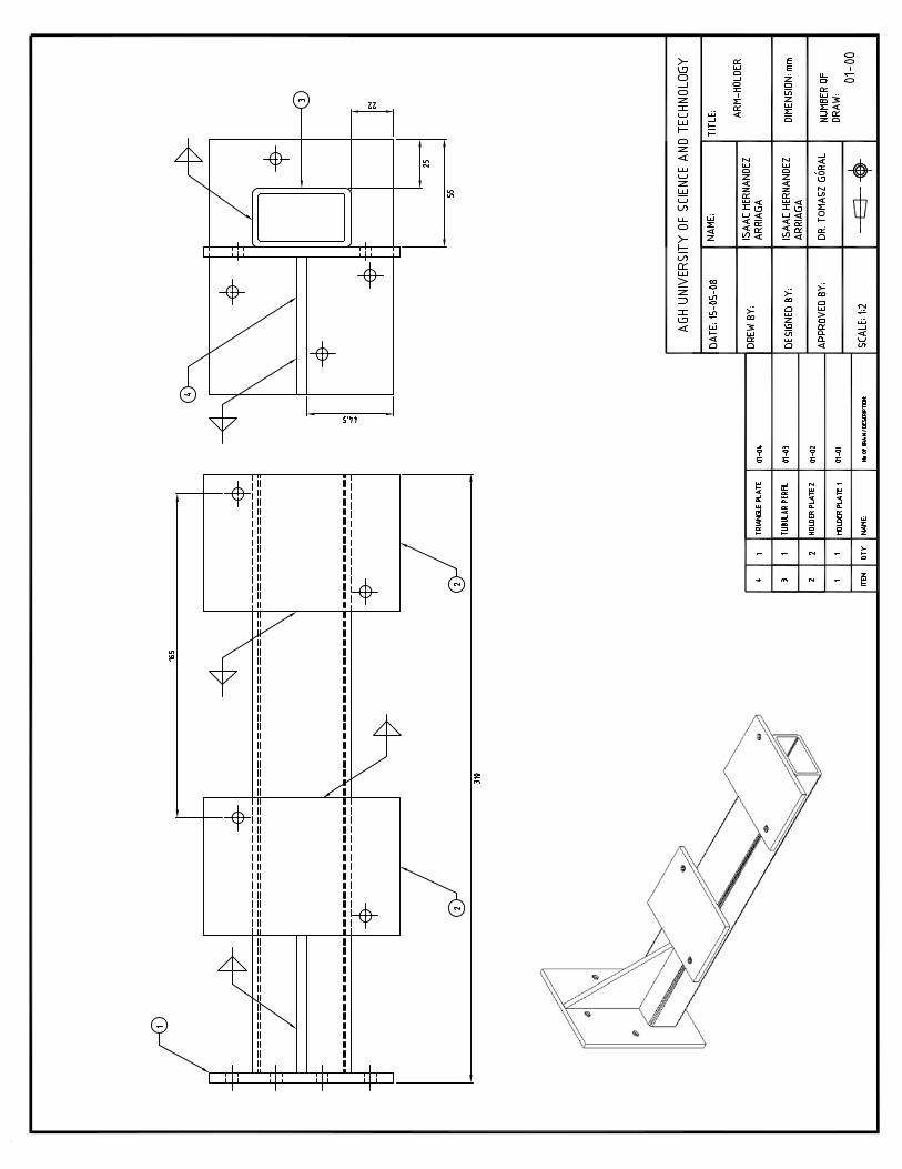
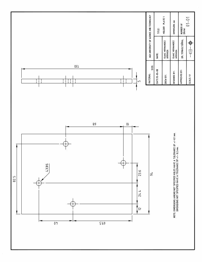
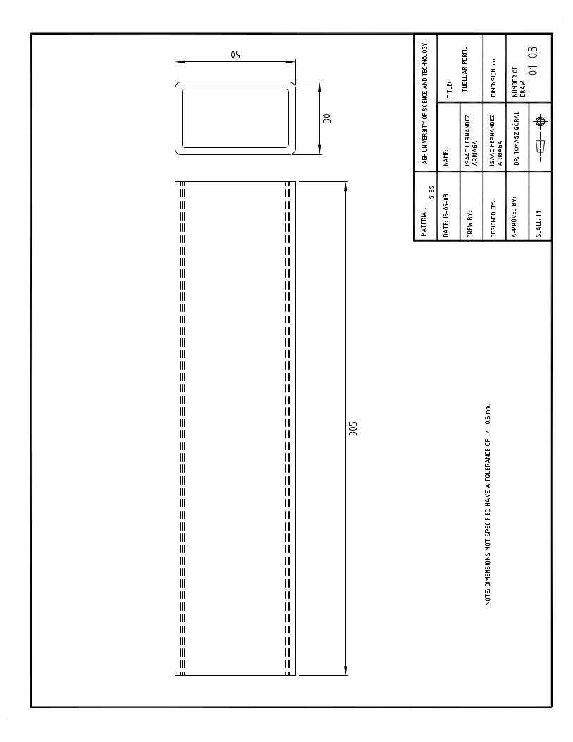
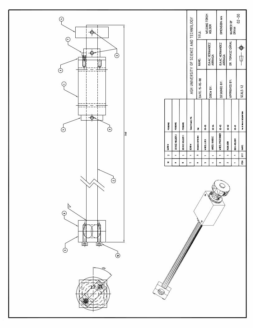
Figure 6.1 Semiautomatic welding machine OPTYMAG 501 112 Figure 6.2 Typical zone of good short circuit welding conditions [37] 113 Figure 6.3 Contact tip to work distance [40] 114 Figure 6.4 Positioning of electrode gun with respect to the base metal plate [37] 114 Figure 6.5 Normal work angle for fillet welds [37] 115 Figure 6.6 Arm-holder device 116 Figure 6.7 Welding torch holder device 117 Figure 6.8 Localization of the locks mounted on the traveler carriage 118 Figure 6.9 Electric oven used to initial residual stresses relief 119 Figure 6.10 Measurement of the initial distortion with standard gages 119 Figure 6.11 Holder-mounting device 120

Welding Sequence Analysis
xvi Isaac Hernández Arriaga
Figure 6.12 Square-mounting device 121 Figure 6.13 C-type clamps mounted on the specimen 122 Figure 6.14 Welding tacks application in the specimen 122 Figure 6.15 Installation of the run-off tabs on the specimen 123 Figure 6.16 Application of the welding to the specimen 124 Figure 6.17 Removing of the run-off tabs of the specimen 125 Figure 6.18 Measurement of the distortion after applying welding using standard gages 125
CHAPTER VII
Figure 7.1 Distortion (exaggerated) after applying welding tacks and after welding for specimen T9 131 Figure 7.2 Distorted shape of the 3-dimensional unitary cell welded specimens 132 Figure 7.3 Final distortion (exaggerated) for welded specimen T9 134
CHAPTER VIII
Figure 8.1 Comparison between numerical (simulation 3) and experimental distortion (specimen
T9). Exaggerated distortion. 139
Figure 8.2 Flow Diagram of the analysis of the welding sequence for symmetrical and asymmetrical structures in 2 and 3 dimensions
144
Welding Sequence Analysis
xvii Isaac Hernández Arriaga
LIST OF TABLES CHAPTER II
Table 2.1 Different welding sequences used by Ji and Fang [17] 17 Table 2.2 Residual stress´s peak value for several cases [17] 18 Table 2.3 Welding sequences and orders applied into the multi-block model [18] 19 Table 2.4 Different welding sequence used by Bart, Deepak and Kyoung [15] 36 Table 2.5 for various welding conditions [23] 40
CHAPTER III Table 3.1 Chemical composition of ASTM A36 carbon steel [33] 56 Table 3.2 Residual stresses obtained in the numerical simulation of I-type specimen subject to
tension 63
Table 3.3 Comparison between numerical data and experimental data of two I-type specimen subject to tension
64
Table 3.4 Welding sequence configuration in the L-type specimen 68 Table 3.5 Distortion at the points of interest in two L-type specimens 74 CHAPTER IV Table 4.1 Welding sequences from the inside to the outside used in the stiffened symmetrical flat
frame 78
Table 4.2 Welding sequences from the outside to the inside used in the stiffened symmetrical flat frame
79
Table 4.3 Order of importance of the analyzed welding sequences in the stiffened symmetrical flat frame
85
Table 4.4 Configuration of welding sequence 5 O-I WT used in the stiffened symmetrical flat specimen
90
Table 4.5 Distortion at the points of interest (mm) in the stiffened symmetrical flat specimen corresponding to welding sequence 5 O-I WT
92
CHAPTER V
Table 5.1 Configuration of the numerical simulations for the 3-dimensional unitary cell 104 Table 5.2 Distortion at 24 points of interest (mm) corresponding to different welding sequences
In the 3-dimensional unitary cell 107
Welding Sequence Analysis
xviii Isaac Hernández Arriaga
Table 5.3 Comparison of numerical results between both welding sequences In the 3-dimensional unitary cell
108
CHAPTER VI
Table 6.1 Electric settings used in the short circuit transfer mode [39] 113 Table 6.2 Common blends of shielding gas composition for short transfer mode [40] 115 CHAPTER VII Table 7.1 3-dimensional unitary cell specimen configuration 128 Table 7.2 Distortion after application of the welding tacks for the different 3-dimensional unitary
cell specimens, mm. 129
Table 7.3 Distortion after welding for the different 3-dimensional unitary cell specimens 24 hrs after welding, mm.
130
Table 7.4 Final distortion in the 24 points of interest of the 3-dimensional unitary cell specimens, mm.
133
CHAPTER VIII Table 8.1 Difference (%) between numerical and experimental results 138
Welding Sequence Analysis
xix Isaac Hernández Arriaga
NOMENCLATURE
Mathematical symbols Units
Rectangular matrix - Column vector, row vector -
Matrix transpose - Matrix inverse -
, Partial differentiation if the following subscript is a letter -
Latin symbols
[ ]B Strain-displacement matrix for each element -
C Specific heat J/Kg°C
[ ]C
Damping matrix Kg/s
Power of viscoplastic straining 1/s Increment of; for example , Tot
ijdε -
epD Elastic-plastic stiffness matrix -
eije Deviation component of elastic strain tensor µε
E Young´s modulus N/m
ijklE
2
Elastic tensor N/m
epijklE
2
Elastic-plastic tensor N/m
tijklE
2
Tangent elastic tensor N/m
if
2
Sum of the body force N
Elastic forces N
Inertia forces N Damping forces N
( ) 0f = Yield surface -
{ }eF Element load vector N
{ }F Global load vector N

Welding Sequence Analysis
xx Isaac Hernández Arriaga
{ }tF Global load vector corresponding at time t N
{ }it tF +∆ Nodal load vector corresponding to the state of stress for the time t∆ -
( )2 1EG
v=
+ Shear modulus N/m
( ) 0G =
2
Plastic potential -
h Convection heat transfer coefficient c W/m2
H°C
Hardening modulus - i Iteration number - kx, ky, k Thermal conductivity in the x, y and z directions z W/m°C
( )3 1 2EK
v=
− Bulk modulus N/m
[ ]K
2
Global stiffness matrix N/m
[ ]eK Element stiffness matrices N/m
tK Stiffness matrix in the time N/m
[ ]M
Mass matrix Kg
n Number of nodal points for each element - ( , , )iN x y z Shape functions -
Nx, Ny, N Cosine directors z - q Boundary heat flux s W/mQ(x,y,z,t)
2 Source of heat generation W/m
{ }tR
3
Nodal point force corresponding at time t -
{ }s Stress deviation increment vector -
s Stress deviation tensor ij N/mT(x,y,z,t)
2 Current temperature °C
Prescribed surface temperature °C T∞ Surrounding temperature °C
mT Melting temperature °C
{ }dTα Thermal dilatation vector -
t∆ Time interval sec
crt∆ Critical time step sec
Displacement vector m
Velocity vector m/s
Acceleration vector m/s2

Welding Sequence Analysis
xxi Isaac Hernández Arriaga
,i ju Displacement gradient -
( )rU Radial distortion with respect to θ mm
Maximun radial distortion mm
{ }U∆ Element nodal increments -
{ }iU∆ Nodal increment vector in the iteration -
{ }Uδ ∆ Admissible virtual nodal increase -
V Volume of the body m
3 Plastic work
Greek symbols α Thermal expansion coefficient µm/m °C
iχ Parameters that control the yield surface size -
δ Kronecker symbol ij - Emissivity
Cauchy strain tensor µε
Power of elastic straining - eijdε Elastic strain increment µε
ekkε Spherical component of elastic strain tensor µε
pijdε Plastic strain increment µε
trijdε Phase transformation strain increment µε
ijd θε Thermal strain increment µε
pdε Equivalent strain increment µε
ijdδ ε Variation in the strain increment µε
κ Parameter related with the strain hardening effects -
dλ Plastic multiplier - v Poisson´s ratio - ρ Density Kg/m
3 Stefan-Boltzmann constant
σ Cauchy stress tensor ij N/mσ
2 Hydrostatic stress tensor kk N/m
2 Spherical invariant N/m
2
Radial residual stress N/m2

Welding Sequence Analysis
xxii Isaac Hernández Arriaga
Von Mises stress N/m or
2 Transverse residual stresses N/m
σ
2 Yield stress y N/m
2 Longitudinal residual stress N/m
2 Axial residual stress N/m
or
2 Circumferential residual stress N/m2

Welding Sequence Analysis
1 Isaac Hernández Arriaga
CHAPTER I
INTRODUCTION
1.1 Background During the heating and cooling cycle in the welding process, thermal strain occurs in the filler material and in the base metal regions close to the weld. The strain produced during heating is accompanied by plastic deformation. The non-uniform plastic deformation that occurs in the weld structure is what leads to residual stresses. These residual stresses react to produce internal forces which must be equilibrated and cause distortion [1]. The residual stress and distortion in weldments depend on several interrelated factors such as thermal cycle, material properties, structural restraints, welding conditions and geometry [2]. Of these parameters, the thermal cycle has the greatest influence on the thermal loads in the welded structures. At the same time, the temperature distribution is a function of parameters such as welding sequence, welding speed, energy of the source, and environmental conditions. A high level of tensile residual stresses near the seam can induce brittle fracture, cracking due to corrosion stress, and reduced fatigue strength. Compressive residual stresses in the base metal located some distance away from the weld line can substantially decrease the critical buckling stress [3]. The main effects of distortion are the loss of tolerance in the welded components and deformation of structural elements that results in inadequate support to transfer applied loads [4]. Therefore, residual stresses and distortion should be reduced to meet all geometry and strength requirements. Some of the most popular methods for reducing residual stresses and distortion in weld fabrication are: welding sequence, definition of weld parameters, definition of weld procedure, use of precambering fixtures, prebending, thermal tensioning, heat sink welding, post-weld treatment, control of weld consumables, and post-weld corrective methods [1].

Welding Sequence Analysis
2 Isaac Hernández Arriaga
1.2 General objective
• Develop a welding sequence-based methodology to reduce residual stresses, distortion, or a relation between both parameters in symmetrical structures.
1.3 Specific Objectives
• Obtain temperature-dependent material properties of ASTM A36 steel used in this investigation.
• Conduct a literature survey on welding sequences.
• Investigate the theory of plasticity applied to the welding process and its finite element formulation.
• Perform a finite element simulation of the welding process through a thermo-mechanical analysis based on the von Mises criterion and flow rule, assuming a lineal isotropic hardening and temperature dependent materials while neglecting micro-structural evolution.
• Validate the proposed numerical model of the welding process with experimental data to determine model accuracy.
• Apply the proposed numerical model of the welding process to determine whether the welding sequence in an L-type structure affects the residual stresses and distortion.
• Apply the proposed numerical model of the welding process in a welding sequence analysis in 2 and 3 dimensional symmetrical structures.
• Analyze the effects of the welding sequence on residual stresses and distortion in 2 and 3 dimensional symmetrical structures.
• Analyze the relationship between residual stress and distortion due to the welding sequence in 2-dimensional symmetrical structures.
• Determine the proper welding sequence to reduce residual stresses, distortion, or a relation between both parameters in 2 and 3 dimensional symmetrical structures.
• Verify if the proper welding sequence for 2-dimensional symmetrical structures is applicable to 3-dimensional symmetrical structures, considering appropriate modifications.
• Develop a methodology for experimental tests.
• Perform experimental tests of the proper welding sequence to reduce distortion in a 2-dimensional symmetrical structure.
• Compare the numerical and experimental results on the proper welding sequence to reduce residual stresses or distortion in a 3-dimensional symmetrical structure.

Welding Sequence Analysis
3 Isaac Hernández Arriaga
CHAPTER II
WELDING SEQUENCE BACKGROUND AND
METHODS FOR CONTROLLING RESIDUAL STRESSES AND DISTORTION INDUCED BY WELDING
2.1 Introduction This chapter presents the methods and advantages of reducing or controlling residual stresses and distortion induced by the welding process as well as a definition and classification of the welding sequence. It also includes a study of the welding sequence analysis, as well as a summary of previous welding sequence research, and a discussion of its advantages, disadvantages, scope, and limitations. 2.2 Advantages of residual stress and distortion control Controlling the residual stress and distortion in weldments provides two main advantages: (1) reduced fabrication costs by minimizing or controlling distortion, and (2) increased service life of the welded structure by controlling the induced residual stress. The benefits of distortion control are [1]: 1. Eliminate the need of expensive distortion correction and loss of accuracy. 2. Reduce machining requirements 3. Improve quality And residual stress control benefits are no less important [2]: 1. Maximize fatigue performance. 2. Minimize costly service problems. 3. Improve resistance to environmental damage.
Welding Sequence Analysis
4 Isaac Hernández Arriaga
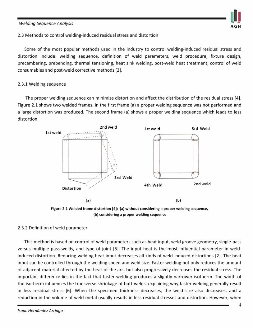
2.3 Methods to control welding-induced residual stress and distortion Some of the most popular methods used in the industry to control welding-induced residual stress and distortion include: welding sequence, definition of weld parameters, weld procedure, fixture design, precambering, prebending, thermal tensioning, heat sink welding, post-weld heat treatment, control of weld consumables and post-weld corrective methods [2]. 2.3.1 Welding sequence The proper welding sequence can minimize distortion and affect the distribution of the residual stress [4]. Figure 2.1 shows two welded frames. In the first frame (a) a proper welding sequence was not performed and a large distortion was produced. The second frame (a) shows a proper welding sequence which leads to less distortion.
Figure 2.1 Welded frame distortion [4]: (a) without considering a proper welding sequence,
(b) considering a proper welding sequence
2.3.2 Definition of weld parameter This method is based on control of weld parameters such as heat input, weld groove geometry, single-pass versus multiple pass welds, and type of joint [5]. The input heat is the most influential parameter in weld-induced distortion. Reducing welding heat input decreases all kinds of weld-induced distortions [2]. The heat input can be controlled through the welding speed and weld size. Faster welding not only reduces the amount of adjacent material affected by the heat of the arc, but also progressively decreases the residual stress. The important difference lies in the fact that faster welding produces a slightly narrower isotherm. The width of the isotherm influences the transverse shrinkage of butt welds, explaining why faster welding generally result in less residual stress [6]. When the specimen thickness decreases, the weld size also decreases, and a reduction in the volume of weld metal usually results in less residual stresses and distortion. However, when

Welding Sequence Analysis
5 Isaac Hernández Arriaga
the specimen thickness decreases, the tensile residual stress in the areas near the fusion zone and distortion increase [6]. This is because thin weldments absorb more energy per unit volume. The use of small groove angles and root openings decrease the volume of weld metal, resulting in lower transverse shrinkage. For example, the use of a U-groove instead of a V-groove should reduce the amount of weld metal [3]. Welding is frequently performed in one pass, especially for thin plates. However, when welding is performed in multiple passes, particularly when welding thick plates, shrinkage accumulates [3]. 2.3.3 Weld procedure Welding procedures have considerable effect on distortion. Fusion welding often leads to the largest distortion, while laser (LBW), electron beam (EBW), and stir welding (FRW) result in lower distortion. However, friction stir welding can impart large plastic strains to the structure. These large strains, which locally strain-harden the material, can influence the fracture response of the structure [8]. In fusion welding, residual stress distributions are similar; this is true when the design and relative size of the weldments are also similar. The most important fusion welding processes are Shield Metal Arc Welding (SMAW), Gas Metal Arc Welding (GMAW), Submerged Arc Welding (SAW), and Gas Tungsten Arc Welding (GTAW). However, the automatic or semiautomatic welding processes present more advantages in the residual stresses and distortion control due to their repeatability. 2.3.4 Fixture design This method is based on the design of clamps, jigs and rigid supports that restrain displacements and rotations of some portions of the welded components or the complete structure. However, the use of these devices increases residual stresses [7,9-10]. Figure 2.2 shows a rigid support formed by a back plate and two clamps. The clamps restrain the angular distortion of the welded joint.
Figure 2.2 Rigid supports [4]
2.3.5 Precambering This method consists on elastically bending some of the components (usually in a specially designed fixture) in a predefined manner before welding. After welding, the precamber is released and the fabricated structure
Welding Sequence Analysis
6 Isaac Hernández Arriaga
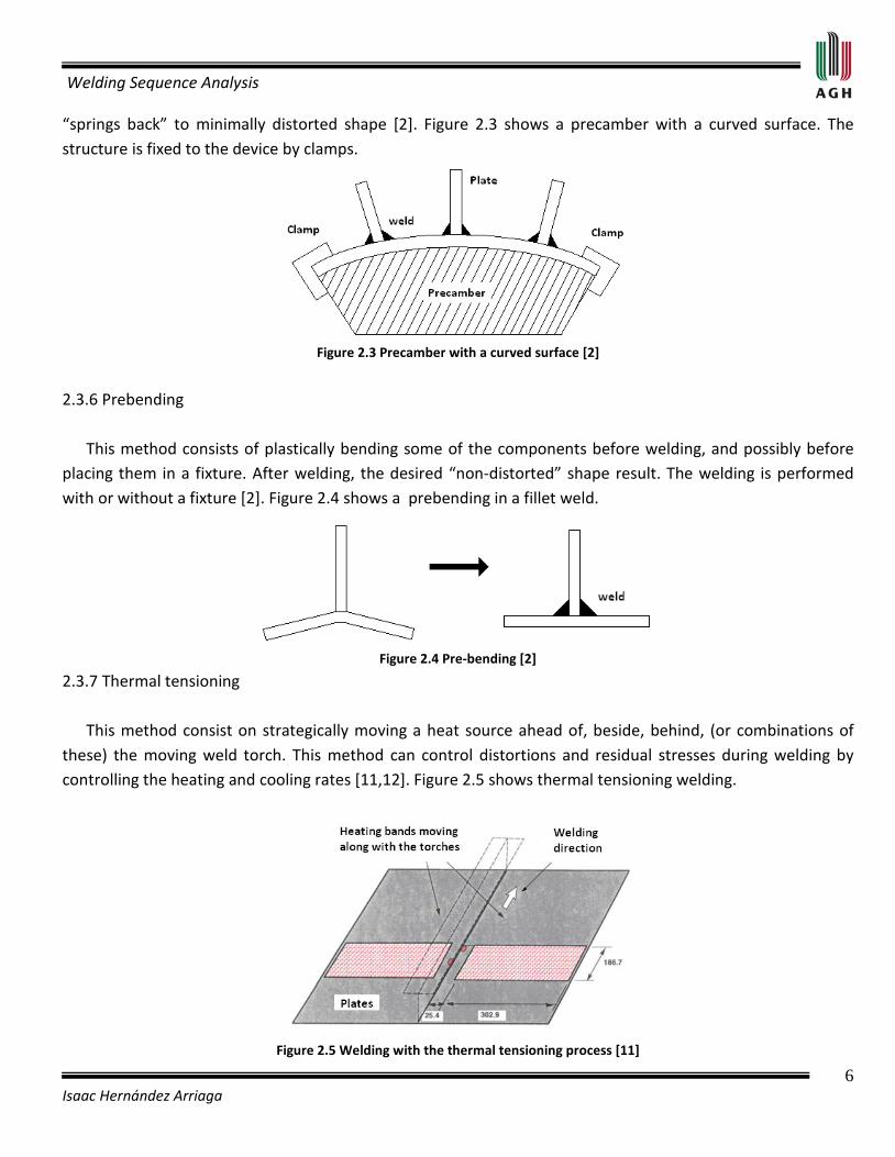
“springs back” to minimally distorted shape [2]. Figure 2.3 shows a precamber with a curved surface. The structure is fixed to the device by clamps.
Figure 2.3 Precamber with a curved surface [2]
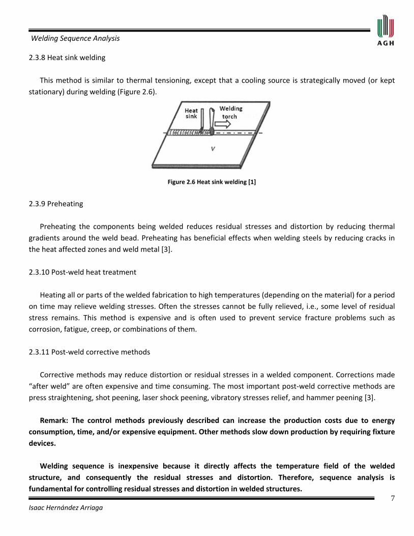
2.3.6 Prebending This method consists of plastically bending some of the components before welding, and possibly before placing them in a fixture. After welding, the desired “non-distorted” shape result. The welding is performed with or without a fixture [2]. Figure 2.4 shows a prebending in a fillet weld.
Figure 2.4 Pre-bending [2]
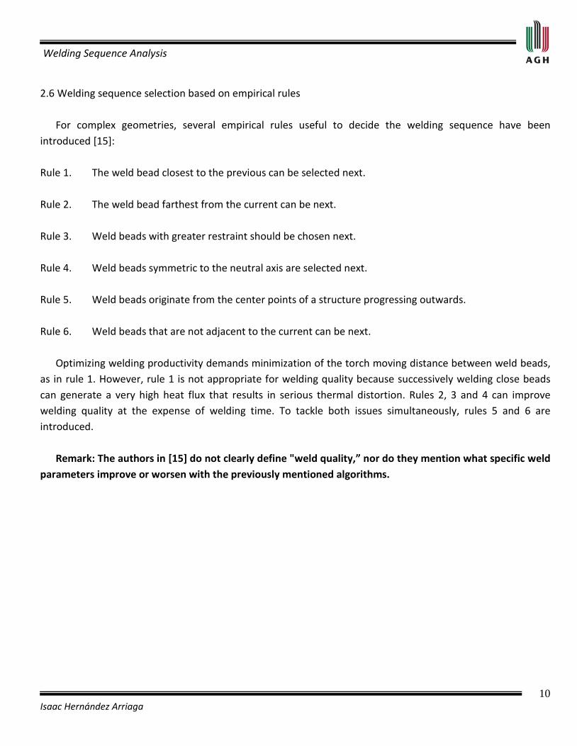
2.3.7 Thermal tensioning This method consist on strategically moving a heat source ahead of, beside, behind, (or combinations of these) the moving weld torch. This method can control distortions and residual stresses during welding by controlling the heating and cooling rates [11,12]. Figure 2.5 shows thermal tensioning welding.
Figure 2.5 Welding with the thermal tensioning process [11]
Welding Sequence Analysis
7 Isaac Hernández Arriaga
2.3.8 Heat sink welding This method is similar to thermal tensioning, except that a cooling source is strategically moved (or kept stationary) during welding (Figure 2.6).
Figure 2.6 Heat sink welding [1]
2.3.9 Preheating Preheating the components being welded reduces residual stresses and distortion by reducing thermal gradients around the weld bead. Preheating has beneficial effects when welding steels by reducing cracks in the heat affected zones and weld metal [3]. 2.3.10 Post-weld heat treatment Heating all or parts of the welded fabrication to high temperatures (depending on the material) for a period on time may relieve welding stresses. Often the stresses cannot be fully relieved, i.e., some level of residual stress remains. This method is expensive and is often used to prevent service fracture problems such as corrosion, fatigue, creep, or combinations of them. 2.3.11 Post-weld corrective methods Corrective methods may reduce distortion or residual stresses in a welded component. Corrections made “after weld” are often expensive and time consuming. The most important post-weld corrective methods are press straightening, shot peening, laser shock peening, vibratory stresses relief, and hammer peening [3]. Remark: The control methods previously described can increase the production costs due to energy consumption, time, and/or expensive equipment. Other methods slow down production by requiring fixture devices. Welding sequence is inexpensive because it directly affects the temperature field of the welded structure, and consequently the residual stresses and distortion. Therefore, sequence analysis is fundamental for controlling residual stresses and distortion in welded structures.

Welding Sequence Analysis
8 Isaac Hernández Arriaga
2.4 Welding sequence definition The American Welding Society (AWS) defines welding sequence as the order of making welds in a weldment [13]. 2.5 Welding sequence classification Welding sequences are classified by the number of passes: single pass and multiple pass weld sequences. However, single pass sequences can be applied to multiple pass welds between beads [3]. 2.5.1 Welding sequence for single pass welds For thin components (up to ¼ inch) welding is performed in a single pass [3]. The weld bead is divided in short sections and welded considering the order and direction of the welds [3,14]. The more common welding sequences for single pass welds are: progressive, backstep, symmetric, and jump (Figure 2.7).
Figure 2.7 Sequences for thin-wall butt-welds [3]: (a) Progressive, (b) backstep, (c) symmetric, and (d) jump
Figure 2.7 (a) corresponds to progressive welding, where the weld beads are set down continually from one end of the joint to the other. In the backstep sequence (Figure 2.7 b), the weld beads are deposited in the opposite direction to the welding progress. Figure 2.7 (c) is the symmetric welding sequence, where the weld beads are deposited from the axis of symmetry of the joint. In the jump welding sequence (Figure 2.7 d) the weld beads are deposited in intermittent form.

Welding Sequence Analysis
9 Isaac Hernández Arriaga
2.5.2 Welding sequence for multiple pass welds For thick components (over 1/4 inch), welding sequences are classified as [3]:
• Built-Up: The first layer is completed along the entire weld length through the previously described single pass sequences (progressive, backstep, symmetric, jump sequences, etc.), followed by the second, third, etc. (Figure 2.8). This sequence applies to large-diameter butt-welded pipe joints frequently used in boiling water reactors, oil pipe transport systems, and steam piping systems.
Figure 2.8 Built-Up welding sequence on thick-wall butt-weld [3]
• Block welding: A given block of the joint is welded completely and then the next block is welded, and so on. This kind of welding sequence is applied mainly to very long joints (e.g., ship hulls). Figure 2.9 shows the block welding sequence on thick-wall butt-weld, where first the end blocks of the joint are welded in, and later the central block is added to the joint.
Figure 2.9 Block welding sequence [3]
• Cascade welding: It is similar to the block welding sequence; the main difference is that the ends of the blocks overlap. An application of this sequence is welding of long thick plates (Figure 2.10).
Figure 2.10 Cascade welding sequence [3]
Welding Sequence Analysis
10 Isaac Hernández Arriaga
2.6 Welding sequence selection based on empirical rules For complex geometries, several empirical rules useful to decide the welding sequence have been introduced [15]: Rule 1. The weld bead closest to the previous can be selected next.
Rule 2. The weld bead farthest from the current can be next.
Rule 3. Weld beads with greater restraint should be chosen next.
Rule 4. Weld beads symmetric to the neutral axis are selected next.
Rule 5. Weld beads originate from the center points of a structure progressing outwards.
Rule 6. Weld beads that are not adjacent to the current can be next. Optimizing welding productivity demands minimization of the torch moving distance between weld beads, as in rule 1. However, rule 1 is not appropriate for welding quality because successively welding close beads can generate a very high heat flux that results in serious thermal distortion. Rules 2, 3 and 4 can improve welding quality at the expense of welding time. To tackle both issues simultaneously, rules 5 and 6 are introduced. Remark: The authors in [15] do not clearly define "weld quality,” nor do they mention what specific weld parameters improve or worsen with the previously mentioned algorithms.
Welding Sequence Analysis
11 Isaac Hernández Arriaga
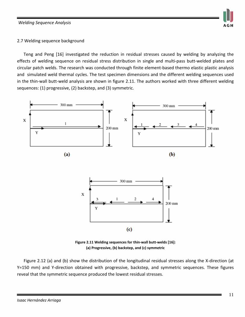
2.7 Welding sequence background Teng and Peng [16] investigated the reduction in residual stresses caused by welding by analyzing the effects of welding sequence on residual stress distribution in single and multi-pass butt-welded plates and circular patch welds. The research was conducted through finite element-based thermo elastic plastic analysis and simulated weld thermal cycles. The test specimen dimensions and the different welding sequences used in the thin-wall butt-weld analysis are shown in figure 2.11. The authors worked with three different welding sequences: (1) progressive, (2) backstep, and (3) symmetric.
Figure 2.11 Welding sequences for thin-wall butt-welds [16]: (a) Progressive, (b) backstep, and (c) symmetric
Figure 2.12 (a) and (b) show the distribution of the longitudinal residual stresses along the X-direction (at Y=150 mm) and Y-direction obtained with progressive, backstep, and symmetric sequences. These figures reveal that the symmetric sequence produced the lowest residual stresses.

Welding Sequence Analysis
12 Isaac Hernández Arriaga
Figure 2.12. Longitudinal residual stress distribution [16]:
(a) Along the X-direction and (b) along the Y-direction

Welding Sequence Analysis
13 Isaac Hernández Arriaga
Reference [16] also considered butt-welded thick plate joints (figure 2.13). Three different cases are considered. Case (A): welding half of the upper groove, the whole lower groove and then the remaining upper groove. Case (B): welding half of the upper groove, half of the lower groove, the remaining of the upper groove and then the remaining lower groove. Case (C): welding the whole lower groove before the whole upper groove.
Figure 2.13 Different welding sequence for thick-wall butt-welds [16]
Figure 2.14 (a) and (b) depict the distribution of the longitudinal and transverse residual stresses obtained with various types of welding sequences. Longitudinal residual stresses between various welding sequences did not appear to differ significantly. However, the transverse residual stresses of case (A) were smaller than those of the other welding sequences. This difference might be attributed to two reasons: (1) the symmetric welding sequence can reduce the residual shrinkage or (2) the symmetric welding sequence has pre-heating and post-heating effects.

Welding Sequence Analysis
14 Isaac Hernández Arriaga
Figure 2.14 Residual stresses distribution along the X-direction in various welding sequences
for thick-wall butt-welds [16]: (a) Longitudinal and (b) transverse

Welding Sequence Analysis
15 Isaac Hernández Arriaga
Finally, the effect of sequences on residual stresses for circular plates is reported [16]. Figure 2.15 shows the various welding sequences for circular patch welds.
Figure 2.15 Geometry and various welding sequence for circular patch [16]:
(a) Geometry of circular patch welding, (b) Progressive sequence, (c) backstep sequence, and (d) jump sequence
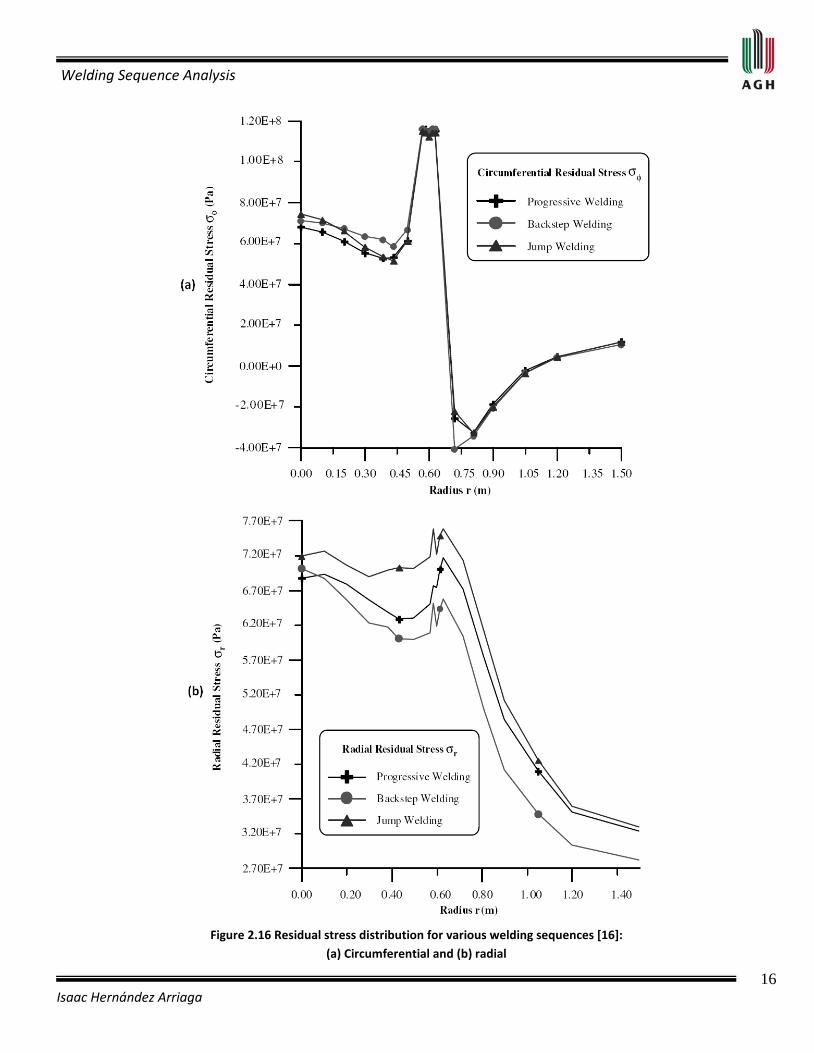
Figure 2.16 (a) depicts the distribution of circumferential residual stresses and reveals that the various welding sequences do not appear to differ significantly. Figure 2.16 (b) depicts the distribution of radial residual stress and reveals that the backstep sequence has smaller radial residual stresses than the other welding sequences. This is because the post-weld treatment and the pre-heating effect of backstep sequence are better than in the other welding sequences. Remark: Reference [16] is applicable only to simple structures, and the numerical simulations do not consider the welding direction. No experiments were conducted for validating the numerical results for the different welding sequences.
Welding Sequence Analysis
16 Isaac Hernández Arriaga
Figure 2.16 Residual stress distribution for various welding sequences [16]:
(a) Circumferential and (b) radial
Welding Sequence Analysis
17 Isaac Hernández Arriaga
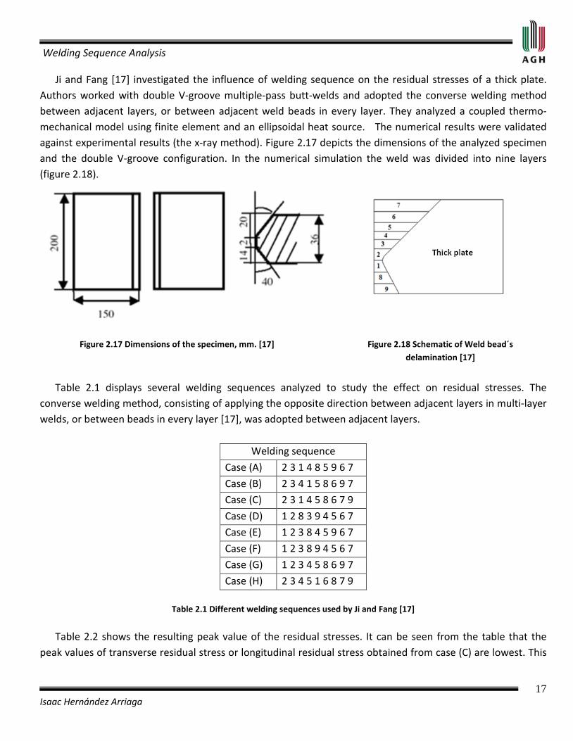
Ji and Fang [17] investigated the influence of welding sequence on the residual stresses of a thick plate. Authors worked with double V-groove multiple-pass butt-welds and adopted the converse welding method between adjacent layers, or between adjacent weld beads in every layer. They analyzed a coupled thermo-mechanical model using finite element and an ellipsoidal heat source. The numerical results were validated against experimental results (the x-ray method). Figure 2.17 depicts the dimensions of the analyzed specimen and the double V-groove configuration. In the numerical simulation the weld was divided into nine layers (figure 2.18).
Figure 2.17 Dimensions of the specimen, mm. [17] Figure 2.18 Schematic of Weld bead´s delamination [17]
Table 2.1 displays several welding sequences analyzed to study the effect on residual stresses. The converse welding method, consisting of applying the opposite direction between adjacent layers in multi-layer welds, or between beads in every layer [17], was adopted between adjacent layers.
Welding sequence
Case (A) 2 3 1 4 8 5 9 6 7
Case (B) 2 3 4 1 5 8 6 9 7
Case (C) 2 3 1 4 5 8 6 7 9
Case (D) 1 2 8 3 9 4 5 6 7
Case (E) 1 2 3 8 4 5 9 6 7
Case (F) 1 2 3 8 9 4 5 6 7
Case (G) 1 2 3 4 5 8 6 9 7
Case (H) 2 3 4 5 1 6 8 7 9
Table 2.1 Different welding sequences used by Ji and Fang [17]
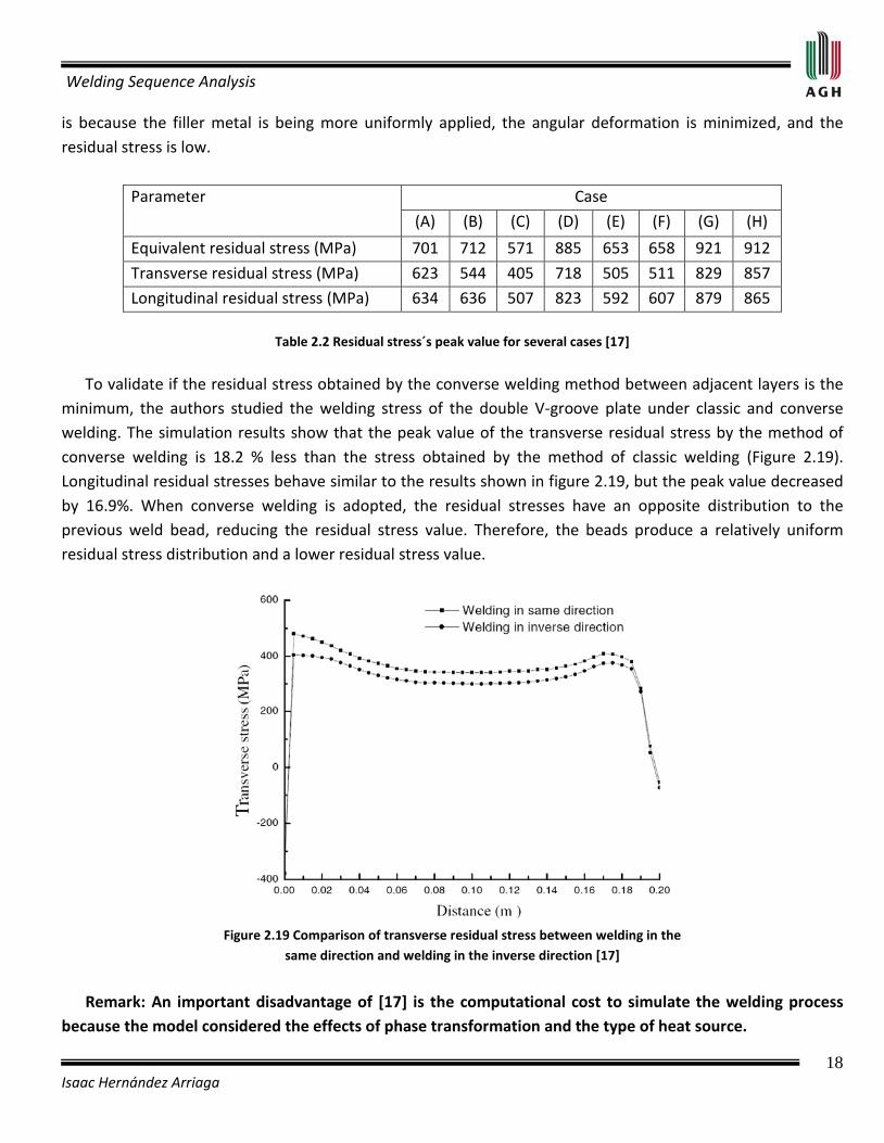
Table 2.2 shows the resulting peak value of the residual stresses. It can be seen from the table that the peak values of transverse residual stress or longitudinal residual stress obtained from case (C) are lowest. This
Welding Sequence Analysis
18 Isaac Hernández Arriaga
is because the filler metal is being more uniformly applied, the angular deformation is minimized, and the residual stress is low.
Parameter Case
(A) (B) (C) (D) (E) (F) (G) (H)
Equivalent residual stress (MPa) 701 712 571 885 653 658 921 912
Transverse residual stress (MPa) 623 544 405 718 505 511 829 857
Longitudinal residual stress (MPa) 634 636 507 823 592 607 879 865
Table 2.2 Residual stress´s peak value for several cases [17]
To validate if the residual stress obtained by the converse welding method between adjacent layers is the minimum, the authors studied the welding stress of the double V-groove plate under classic and converse welding. The simulation results show that the peak value of the transverse residual stress by the method of converse welding is 18.2 % less than the stress obtained by the method of classic welding (Figure 2.19). Longitudinal residual stresses behave similar to the results shown in figure 2.19, but the peak value decreased by 16.9%. When converse welding is adopted, the residual stresses have an opposite distribution to the previous weld bead, reducing the residual stress value. Therefore, the beads produce a relatively uniform residual stress distribution and a lower residual stress value.
Figure 2.19 Comparison of transverse residual stress between welding in the
same direction and welding in the inverse direction [17]
Remark: An important disadvantage of [17] is the computational cost to simulate the welding process because the model considered the effects of phase transformation and the type of heat source.

Welding Sequence Analysis
19 Isaac Hernández Arriaga
Nami, Kadivar and Jafarpur [18] studied the welding sequence in multiple blocks for the effect on the thermal and mechanical response of thick plate weldments by the use of a 3-D thermo-viscoplastic model. Anand´s viscoplastic model was used to simulate the rate dependent plastic deformation of welded materials. Also, they considered the temperature dependence of thermal and mechanical properties of material, welding speed, welding lag, and the effect of the filling material added to the weld. The model was compared with the results of two analytical and experimental works. Figure 2.20 depicts the configuration and dimensions of the welded blocks. The length of the welded strip was divided into seven parts and welded by different sequences. The arc was allowed to move in a forward (+X3) or in a backward direction (-X3). Figure 2.21 depicts the structural boundary conditions of the welded plates.
Figure 2.20 Configuration of welded blocks in Figure 2.21 Structural boundary conditions of welded a multi-block welding sequence [18] plates (clamp fixture at both sides) [18]
The selected welding sequences in table 2.3 are commonly used in practice. In the first sequence the joining was done inwardly (toward the center of the plates) and in second sequence the joining happened toward the edge of the plates (outwardly).
Table 2.3 Welding sequences and orders applied into the multi-block model [18]
Welding sequence Configuration
1 +1, +7, +2, +6, +3, +5, -4
2 +2, +4, +6, +1, +3, +5,+7
Welding Sequence Analysis
20 Isaac Hernández Arriaga
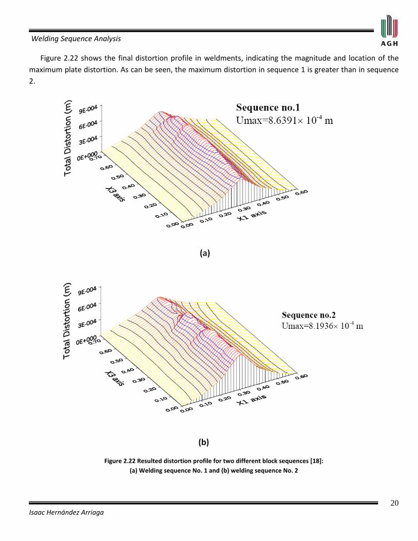
Figure 2.22 shows the final distortion profile in weldments, indicating the magnitude and location of the maximum plate distortion. As can be seen, the maximum distortion in sequence 1 is greater than in sequence 2.
Figure 2.22 Resulted distortion profile for two different block sequences [18]:
(a) Welding sequence No. 1 and (b) welding sequence No. 2
Welding Sequence Analysis
21 Isaac Hernández Arriaga
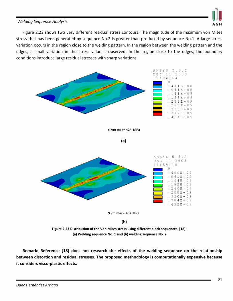
Figure 2.23 shows two very different residual stress contours. The magnitude of the maximum von Mises stress that has been generated by sequence No.2 is greater than produced by sequence No.1. A large stress variation occurs in the region close to the welding pattern. In the region between the welding pattern and the edges, a small variation in the stress value is observed. In the region close to the edges, the boundary conditions introduce large residual stresses with sharp variations.
Figure 2.23 Distribution of the Von Mises stress using different block sequences. [18]:
(a) Welding sequence No. 1 and (b) welding sequence No. 2
Remark: Reference [18] does not research the effects of the welding sequence on the relationship between distortion and residual stresses. The proposed methodology is computationally expensive because it considers visco-plastic effects.

Welding Sequence Analysis
22 Isaac Hernández Arriaga
Mochizuki and Hayashi [19] investigated the residual stress in large-diameter, multi-pass, butt-welded pipe joints for various welding sequences. The pipe joints had an x-shaped groove. The mechanism that produces residual stress in the welded pipe joints was studied in detail using a simple prediction model. The authors worked with a thermo-elastic-plastic analysis using finite element method with an axisymmetric model. Also, they determined an optimum welding sequence for preventing stress-corrosion cracking from the residual stress distribution. The configuration of a large-diameter, multi-pass, butt-welded pipe joint and its cross section is shown in figure 2.24.
Figure 2.24 Configuration of a large-diameter multi-pass Figure 2.25 Welding sequences for a multi-pass pass butt-welded pipe joints and its cross section [19] Welded pipe joint [19]
The authors [19] proposed six welding sequences (figure 2.25) to study the dependence of the residual stress on the welding sequence. In case 1 the inner side of the groove is welded before the outer surface of the groove. In case 2, the outer side of the groove is welded before the inner surface of the groove. In case 3, half of the inner side of the groove is welded, then the whole outer side, and later the remaining inner side groove. In case 4, half of the outer side of the groove is welded, then the whole inner side of the groove, and later the remaining outer groove. In case 5, half of the inner side of the groove is welded, then half of the outer groove, later the remaining inner groove, and lastly the remaining outer groove. In case 6, half of the outside groove is welded, then half of the inside groove, later the remaining outside groove and at the end the remaining inside groove.
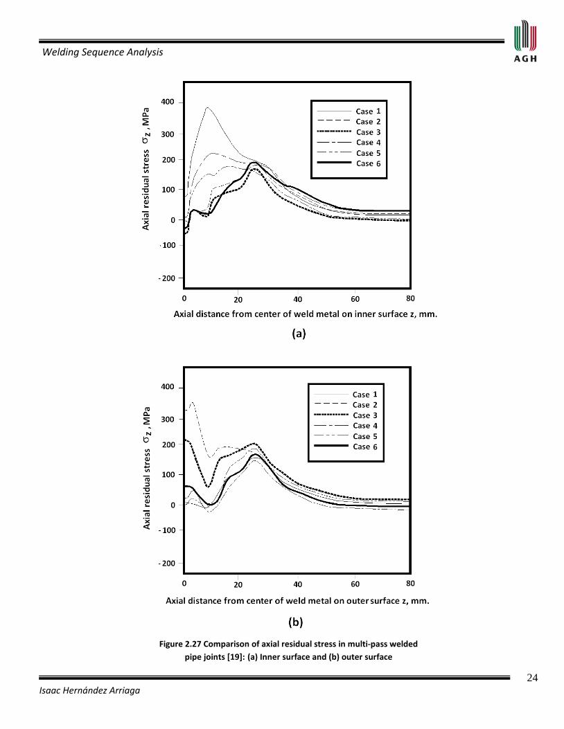
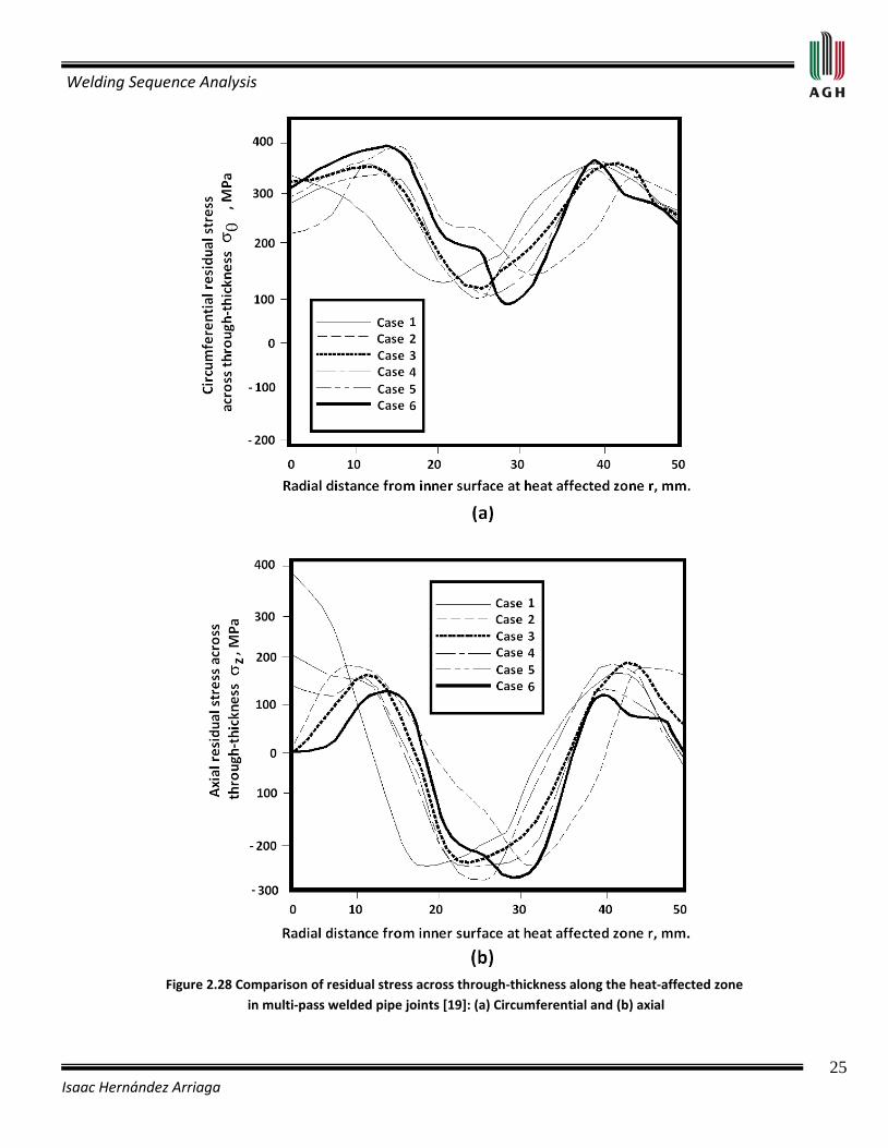
Figure 2.26 (a) and (b) show a comparison between the circumferential residual stresses on the inner and outer surfaces of the groove; Figure 2.27 (a) and (b) show a comparison of the axial residual stresses on the inner and outer surfaces of the groove; and Figure 2.28 (a) and (b) show a comparison between the circumferential and axial residual stresses through the plate thickness along the heat-affected zone. All these figures consider multi-pass, butt-welded, pipe joints.

Welding Sequence Analysis
23 Isaac Hernández Arriaga
Figure 2.26 Comparison of circumferential residual stress in multi-pass welded
pipe joints [19]: (a) Inner surface and (b) outer surface
Welding Sequence Analysis
24 Isaac Hernández Arriaga
Figure 2.27 Comparison of axial residual stress in multi-pass welded
pipe joints [19]: (a) Inner surface and (b) outer surface
Welding Sequence Analysis
25 Isaac Hernández Arriaga
Figure 2.28 Comparison of residual stress across through-thickness along the heat-affected zone
in multi-pass welded pipe joints [19]: (a) Circumferential and (b) axial

Welding Sequence Analysis
26 Isaac Hernández Arriaga
In figures 2.26 (a), 2.26 (b) and 2.28 (a), the circumferential residual stresses behaved similarly: tensile circumferential stresses are distributed near the welding deposit on the inner and outer surfaces. The maximum stress occurs near the welded metal. Tensile stress then decreases and finally becomes compressive about 40 mm from the center of welded metal. In figures 2.27 (a), 2.27 (b) and 2.28 (b), the distribution of the axial residual stress near the welding deposit differs depending on the welding sequence. Stresses in the heat-affected zone vary with the welding sequence, both on the surface and through the thickness, but the axial residual stress distribution away from the welded metal is not affected by the welding sequence.
Through-thickness axial residual stresses along the heat-affected zone have a big influence in the generation and propagation of stress-corrosion cracking in multi-pass, welded pipe joints. The inner surface is exposed to a more severe environment than the outer surface because the pipe may contain corrosive substances. There are two steps in selecting an optimum welding sequence for preventing stress-corrosion cracking: (i) lowering the axial residual stress on the inner surface along the heat-affected zone, because crack generation should be prevented first; and (ii) lowering the through-thickness axial stress near the inner surface to reduce or eliminate crack propagation rate, even if a crack begins to propagate. According to figure 2.28 (b), cases 2, 3, and 6 are good candidates since they produced lower stresses on the inner surface of the heat affected zone. Among these, case 6 was the best because the axial through-thickness stress near the inner surface is almost zero up to a depth of 6 mm. This welding sequence should have the lowest probability of generating and propagating stress-corrosion cracking. Remark: In the work performed by Mochizuki and Hayashi [19], the analytical method proposed to determine the residual stresses through-thickness is only applicable to multi-pass, welded pipe joints. Therefore, the method is not valid for pipe joints of small diameter (single pass joints). The method presented has a good qualitative correlation with experimental and numerical data. However, quantitative correlation was not good.

Welding Sequence Analysis
27 Isaac Hernández Arriaga
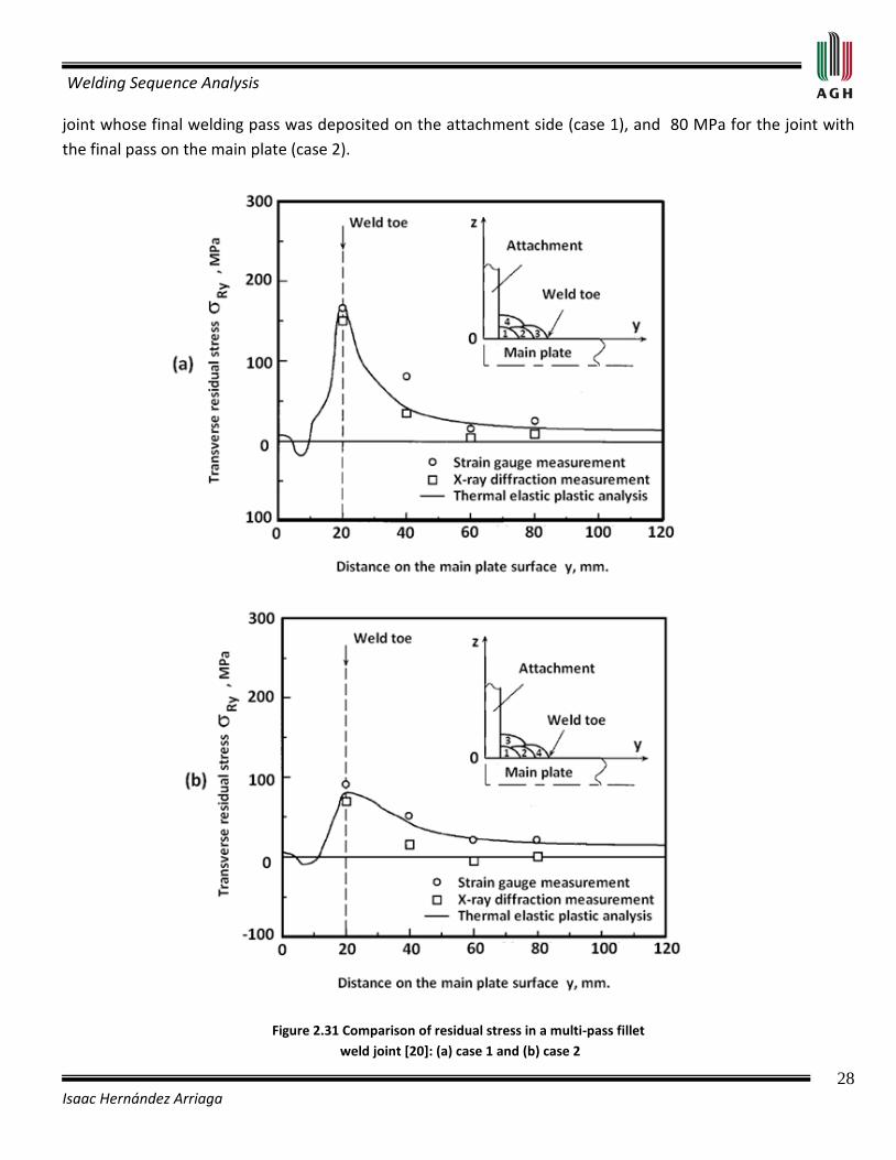
Mochizuki, Hattori and Nakakado [20] studied the effect of residual stress on fatigue strength at a weld toe in a multi-pass fillet weld joint. The residual stress in the specimen was varied by controlling the welding sequence. They calculated the residual stresses by thermo-elastic-plastic analysis and compared them to strain gage and X-ray diffraction measurements. A weld joint was fabricated to evaluate the residual stress and fatigue strength. Two attachments were fillet-welded on both sides of a main plate, as shown in figure 2.29.
Figure 2.29 Configuration of a multi-pass fillet Weld joint, mm. [20]
Two joints were fabricated by changing the welding sequence, as shown in figure 2.30. In case 1, the final welding pass was set down in the attachment side, and in case 2 the final welding pass was set down in the main plate side.
Figure 2.30 Different welding sequences in multi-pass fillet weld joint [20]
Figure 2.31 depicts the experimental and numerical results for transverse residual stresses for the two welding sequences. The measured and analytical distributions of residual stress agree well. Therefore, the results from the thermo-elastic-plastic analysis were used to define the residual stress needed to evaluate fatigue strength. The transverse residual stress in the weld toe of the main plate was 170 MPa for the weld
Welding Sequence Analysis
28 Isaac Hernández Arriaga
joint whose final welding pass was deposited on the attachment side (case 1), and 80 MPa for the joint with the final pass on the main plate (case 2).
Figure 2.31 Comparison of residual stress in a multi-pass fillet weld joint [20]: (a) case 1 and (b) case 2
Welding Sequence Analysis
29 Isaac Hernández Arriaga
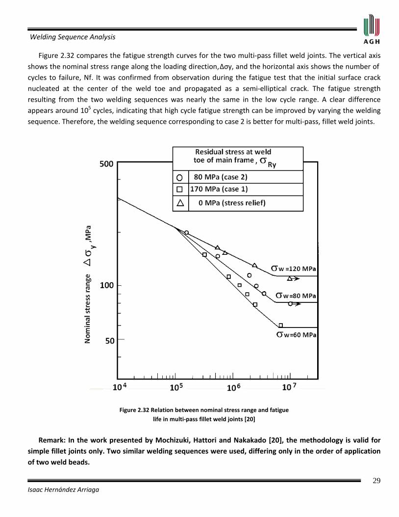
Figure 2.32 compares the fatigue strength curves for the two multi-pass fillet weld joints. The vertical axis shows the nominal stress range along the loading direction, ∆σy, and the horizontal axis shows the number of cycles to failure, Nf. It was confirmed from observation during the fatigue test that the initial surface crack nucleated at the center of the weld toe and propagated as a semi-elliptical crack. The fatigue strength resulting from the two welding sequences was nearly the same in the low cycle range. A clear difference appears around 105
Figure 2.32 Relation between nominal stress range and fatigue life in multi-pass fillet weld joints [20]
Remark: In the work presented by Mochizuki, Hattori and Nakakado [20], the methodology is valid for simple fillet joints only. Two similar welding sequences were used, differing only in the order of application of two weld beads.
cycles, indicating that high cycle fatigue strength can be improved by varying the welding sequence. Therefore, the welding sequence corresponding to case 2 is better for multi-pass, fillet weld joints.
Welding Sequence Analysis
30 Isaac Hernández Arriaga
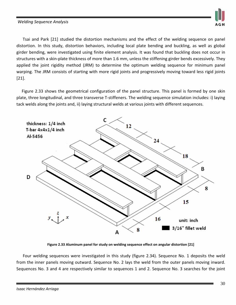
Tsai and Park [21] studied the distortion mechanisms and the effect of the welding sequence on panel distortion. In this study, distortion behaviors, including local plate bending and buckling, as well as global girder bending, were investigated using finite element analysis. It was found that buckling does not occur in structures with a skin-plate thickness of more than 1.6 mm, unless the stiffening girder bends excessively. They applied the joint rigidity method (JRM) to determine the optimum welding sequence for minimum panel warping. The JRM consists of starting with more rigid joints and progressively moving toward less rigid joints [21]. Figure 2.33 shows the geometrical configuration of the panel structure. This panel is formed by one skin plate, three longitudinal, and three transverse T-stiffeners. The welding sequence simulation includes: i) laying tack welds along the joints and, ii) laying structural welds at various joints with different sequences.
Figure 2.33 Aluminum panel for study on welding sequence effect on angular distortion [21]
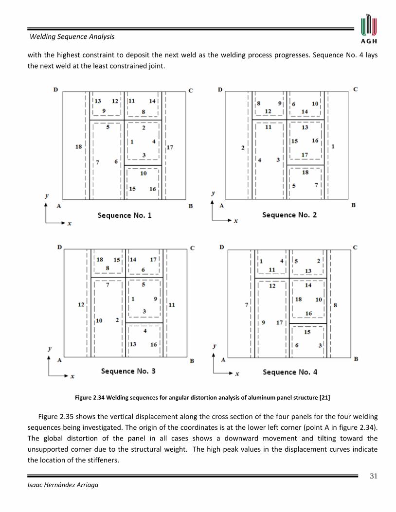
Four welding sequences were investigated in this study (figure 2.34). Sequence No. 1 deposits the weld from the inner panels moving outward. Sequence No. 2 lays the weld from the outer panels moving inward. Sequences No. 3 and 4 are respectively similar to sequences 1 and 2. Sequence No. 3 searches for the joint
Welding Sequence Analysis
31 Isaac Hernández Arriaga
with the highest constraint to deposit the next weld as the welding process progresses. Sequence No. 4 lays the next weld at the least constrained joint.
Figure 2.34 Welding sequences for angular distortion analysis of aluminum panel structure [21]
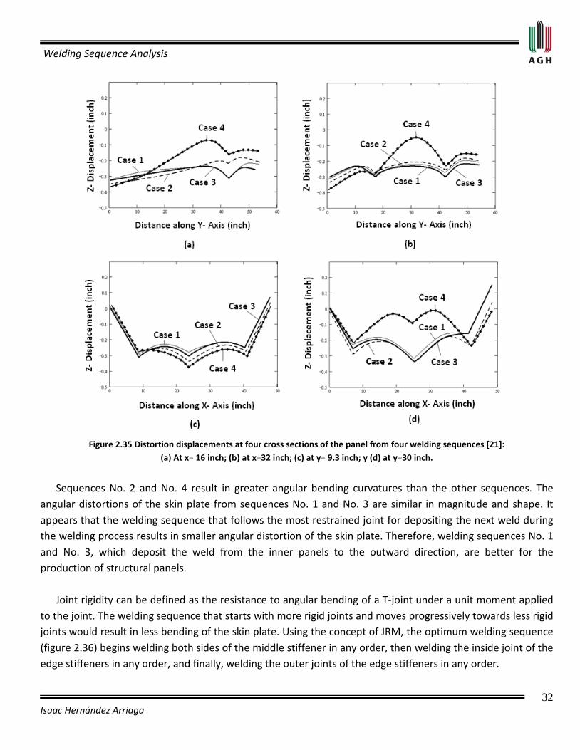
Figure 2.35 shows the vertical displacement along the cross section of the four panels for the four welding sequences being investigated. The origin of the coordinates is at the lower left corner (point A in figure 2.34). The global distortion of the panel in all cases shows a downward movement and tilting toward the unsupported corner due to the structural weight. The high peak values in the displacement curves indicate the location of the stiffeners.
Welding Sequence Analysis
32 Isaac Hernández Arriaga
Figure 2.35 Distortion displacements at four cross sections of the panel from four welding sequences [21]:
(a) At x= 16 inch; (b) at x=32 inch; (c) at y= 9.3 inch; y (d) at y=30 inch.
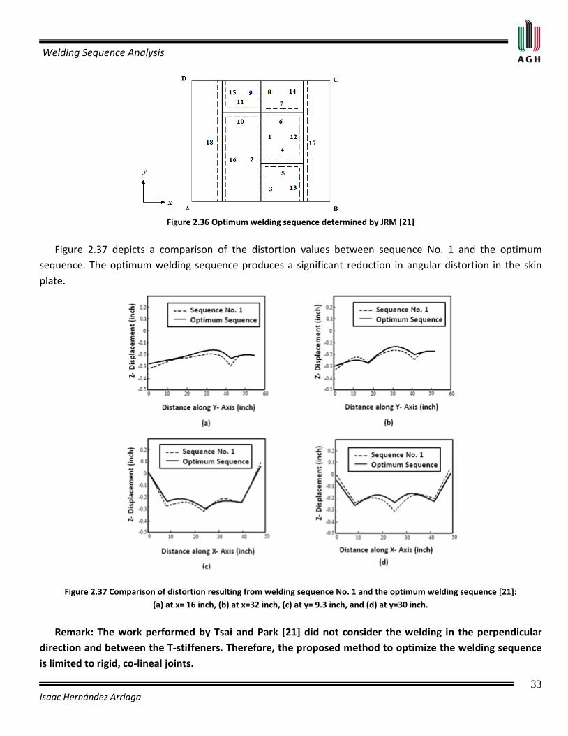
Sequences No. 2 and No. 4 result in greater angular bending curvatures than the other sequences. The angular distortions of the skin plate from sequences No. 1 and No. 3 are similar in magnitude and shape. It appears that the welding sequence that follows the most restrained joint for depositing the next weld during the welding process results in smaller angular distortion of the skin plate. Therefore, welding sequences No. 1 and No. 3, which deposit the weld from the inner panels to the outward direction, are better for the production of structural panels. Joint rigidity can be defined as the resistance to angular bending of a T-joint under a unit moment applied to the joint. The welding sequence that starts with more rigid joints and moves progressively towards less rigid joints would result in less bending of the skin plate. Using the concept of JRM, the optimum welding sequence (figure 2.36) begins welding both sides of the middle stiffener in any order, then welding the inside joint of the edge stiffeners in any order, and finally, welding the outer joints of the edge stiffeners in any order.
Welding Sequence Analysis
33 Isaac Hernández Arriaga
Figure 2.36 Optimum welding sequence determined by JRM [21]
Figure 2.37 depicts a comparison of the distortion values between sequence No. 1 and the optimum sequence. The optimum welding sequence produces a significant reduction in angular distortion in the skin plate.
Figure 2.37 Comparison of distortion resulting from welding sequence No. 1 and the optimum welding sequence [21]: (a) at x= 16 inch, (b) at x=32 inch, (c) at y= 9.3 inch, and (d) at y=30 inch.
Remark: The work performed by Tsai and Park [21] did not consider the welding in the perpendicular direction and between the T-stiffeners. Therefore, the proposed method to optimize the welding sequence is limited to rigid, co-lineal joints.
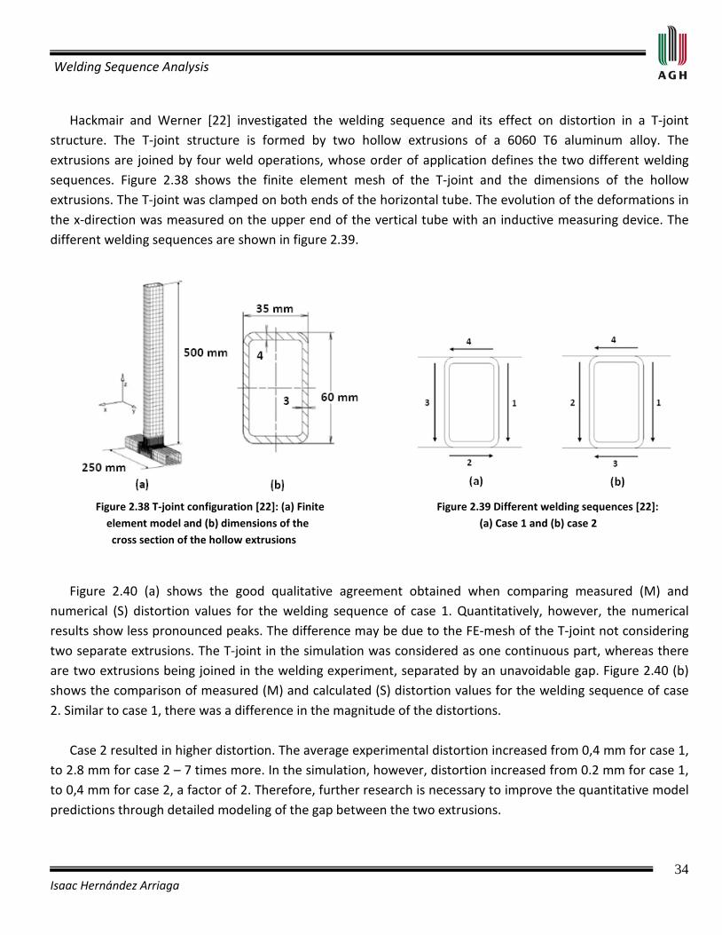
Welding Sequence Analysis
34 Isaac Hernández Arriaga
Hackmair and Werner [22] investigated the welding sequence and its effect on distortion in a T-joint structure. The T-joint structure is formed by two hollow extrusions of a 6060 T6 aluminum alloy. The extrusions are joined by four weld operations, whose order of application defines the two different welding sequences. Figure 2.38 shows the finite element mesh of the T-joint and the dimensions of the hollow extrusions. The T-joint was clamped on both ends of the horizontal tube. The evolution of the deformations in the x-direction was measured on the upper end of the vertical tube with an inductive measuring device. The different welding sequences are shown in figure 2.39.
Figure 2.38 T-joint configuration [22]: (a) Finite Figure 2.39 Different welding sequences [22]: element model and (b) dimensions of the (a) Case 1 and (b) case 2 cross section of the hollow extrusions
Figure 2.40 (a) shows the good qualitative agreement obtained when comparing measured (M) and numerical (S) distortion values for the welding sequence of case 1. Quantitatively, however, the numerical results show less pronounced peaks. The difference may be due to the FE-mesh of the T-joint not considering two separate extrusions. The T-joint in the simulation was considered as one continuous part, whereas there are two extrusions being joined in the welding experiment, separated by an unavoidable gap. Figure 2.40 (b) shows the comparison of measured (M) and calculated (S) distortion values for the welding sequence of case 2. Similar to case 1, there was a difference in the magnitude of the distortions. Case 2 resulted in higher distortion. The average experimental distortion increased from 0,4 mm for case 1, to 2.8 mm for case 2 – 7 times more. In the simulation, however, distortion increased from 0.2 mm for case 1, to 0,4 mm for case 2, a factor of 2. Therefore, further research is necessary to improve the quantitative model predictions through detailed modeling of the gap between the two extrusions.
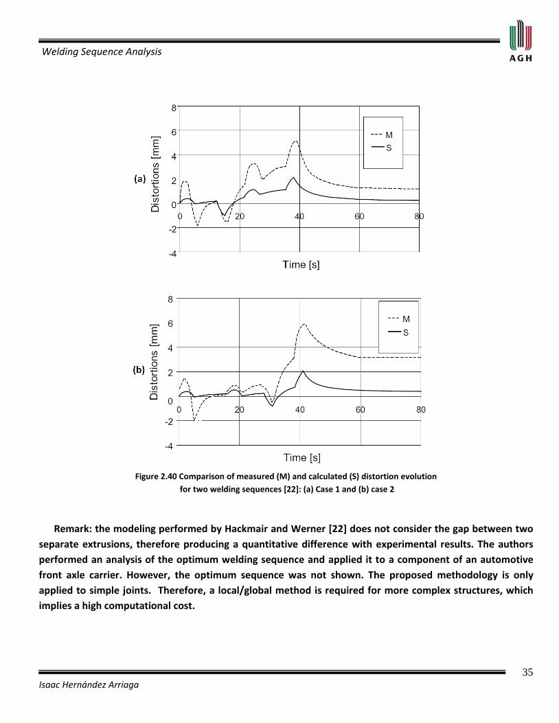
Welding Sequence Analysis
35 Isaac Hernández Arriaga
Figure 2.40 Comparison of measured (M) and calculated (S) distortion evolution
for two welding sequences [22]: (a) Case 1 and (b) case 2
Remark: the modeling performed by Hackmair and Werner [22] does not consider the gap between two separate extrusions, therefore producing a quantitative difference with experimental results. The authors performed an analysis of the optimum welding sequence and applied it to a component of an automotive front axle carrier. However, the optimum sequence was not shown. The proposed methodology is only applied to simple joints. Therefore, a local/global method is required for more complex structures, which implies a high computational cost.
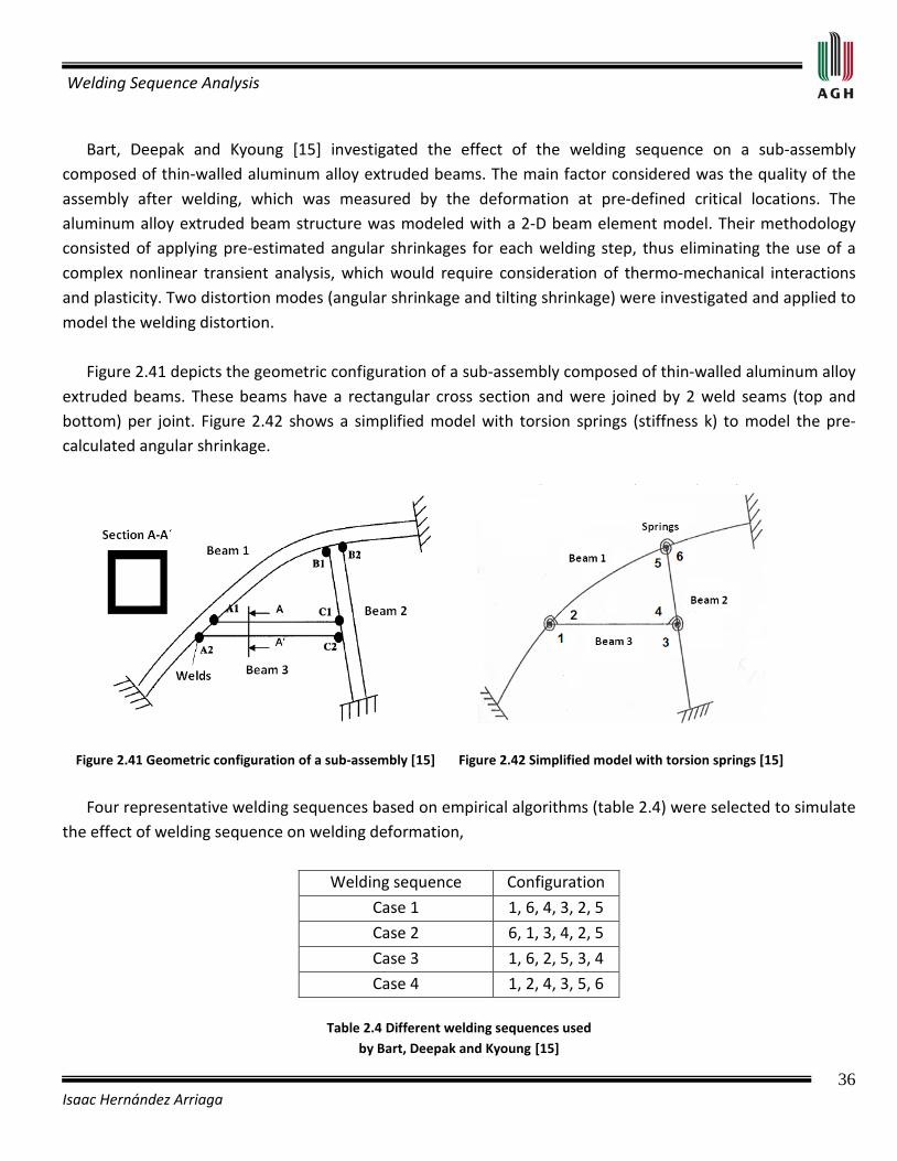
Welding Sequence Analysis
36 Isaac Hernández Arriaga
Bart, Deepak and Kyoung [15] investigated the effect of the welding sequence on a sub-assembly composed of thin-walled aluminum alloy extruded beams. The main factor considered was the quality of the assembly after welding, which was measured by the deformation at pre-defined critical locations. The aluminum alloy extruded beam structure was modeled with a 2-D beam element model. Their methodology consisted of applying pre-estimated angular shrinkages for each welding step, thus eliminating the use of a complex nonlinear transient analysis, which would require consideration of thermo-mechanical interactions and plasticity. Two distortion modes (angular shrinkage and tilting shrinkage) were investigated and applied to model the welding distortion. Figure 2.41 depicts the geometric configuration of a sub-assembly composed of thin-walled aluminum alloy extruded beams. These beams have a rectangular cross section and were joined by 2 weld seams (top and bottom) per joint. Figure 2.42 shows a simplified model with torsion springs (stiffness k) to model the pre-calculated angular shrinkage.
Figure 2.41 Geometric configuration of a sub-assembly [15] Figure 2.42 Simplified model with torsion springs [15]
Four representative welding sequences based on empirical algorithms (table 2.4) were selected to simulate the effect of welding sequence on welding deformation,
Welding sequence Configuration
Case 1 1, 6, 4, 3, 2, 5
Case 2 6, 1, 3, 4, 2, 5
Case 3 1, 6, 2, 5, 3, 4
Case 4 1, 2, 4, 3, 5, 6
Table 2.4 Different welding sequences used by Bart, Deepak and Kyoung [15]
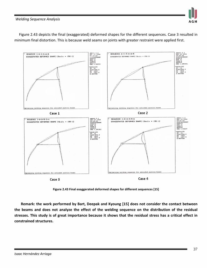
Welding Sequence Analysis
37 Isaac Hernández Arriaga
Figure 2.43 depicts the final (exaggerated) deformed shapes for the different sequences. Case 3 resulted in minimum final distortion. This is because weld seams on joints with greater restraint were applied first.
Figure 2.43 Final exaggerated deformed shapes for different sequences [15]
Remark: the work performed by Bart, Deepak and Kyoung [15] does not consider the contact between the beams and does not analyze the effect of the welding sequence on the distribution of the residual stresses. This study is of great importance because it shows that the residual stress has a critical effect in constrained structures.
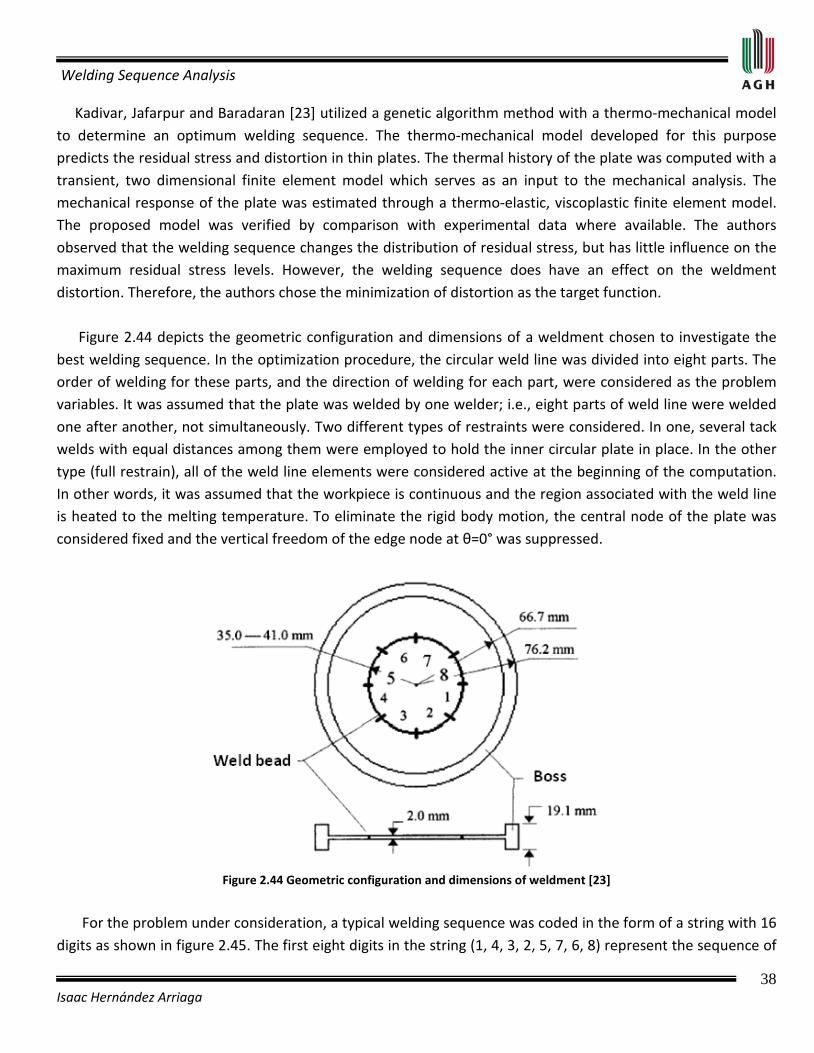
Welding Sequence Analysis
38 Isaac Hernández Arriaga
Kadivar, Jafarpur and Baradaran [23] utilized a genetic algorithm method with a thermo-mechanical model to determine an optimum welding sequence. The thermo-mechanical model developed for this purpose predicts the residual stress and distortion in thin plates. The thermal history of the plate was computed with a transient, two dimensional finite element model which serves as an input to the mechanical analysis. The mechanical response of the plate was estimated through a thermo-elastic, viscoplastic finite element model. The proposed model was verified by comparison with experimental data where available. The authors observed that the welding sequence changes the distribution of residual stress, but has little influence on the maximum residual stress levels. However, the welding sequence does have an effect on the weldment distortion. Therefore, the authors chose the minimization of distortion as the target function. Figure 2.44 depicts the geometric configuration and dimensions of a weldment chosen to investigate the best welding sequence. In the optimization procedure, the circular weld line was divided into eight parts. The order of welding for these parts, and the direction of welding for each part, were considered as the problem variables. It was assumed that the plate was welded by one welder; i.e., eight parts of weld line were welded one after another, not simultaneously. Two different types of restraints were considered. In one, several tack welds with equal distances among them were employed to hold the inner circular plate in place. In the other type (full restrain), all of the weld line elements were considered active at the beginning of the computation. In other words, it was assumed that the workpiece is continuous and the region associated with the weld line is heated to the melting temperature. To eliminate the rigid body motion, the central node of the plate was considered fixed and the vertical freedom of the edge node at θ=0° was suppressed.
Figure 2.44 Geometric configuration and dimensions of weldment [23]
For the problem under consideration, a typical welding sequence was coded in the form of a string with 16 digits as shown in figure 2.45. The first eight digits in the string (1, 4, 3, 2, 5, 7, 6, 8) represent the sequence of

Welding Sequence Analysis
39 Isaac Hernández Arriaga
welding. The second eight digits (1, 2, 2, 2, 1, 2, 2, 1) represent the direction of welding, where 1 and 2 respectively mean clockwise or counterclockwise.
Figure 2.45 Code to designate the welding sequence
and welding direction [23]
As stated earlier, the effects of the welding sequence on the maximum residual stress values are negligible. Therefore, the distortion of the weldment was considered as the objective function. Because the plate was thin, and its deformation was modeled with an in-plane model, the maximum radial displacement at the edge
of the plate ( )maxrU represented the maximum radial weldment distortion.
Figure 2.46 shows the variation of ( )rU with respect to θ when using tack welds. The displacement
produced by the optimum sequence is nearly uniform. In other words, when the optimum sequence is applied, the deformed shape of the plate remains circular with a small contraction; whereas using a continuous sequence the deformed shape of the plate is irregular and with a distorted shape. The maximum displacement
at the edge of the plate ( )maxrU for the optimum sequence was about 70% less than that of the continuous
sequence. Similar results were obtained for the case of welding with full restrain (without tack welds).
Figure 2.46 Radial displacement of the edge of plate with respect to θ
for continuous welding and the optimum sequence[23]
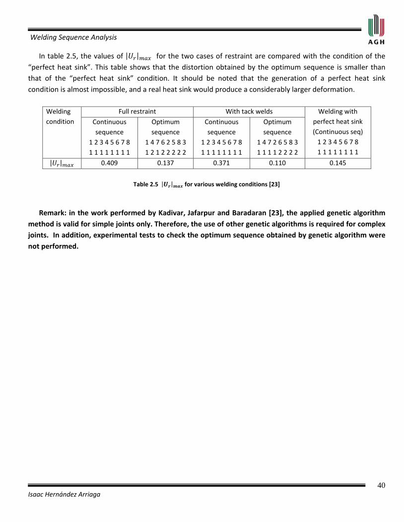
Welding Sequence Analysis
40 Isaac Hernández Arriaga
In table 2.5, the values of for the two cases of restraint are compared with the condition of the “perfect heat sink”. This table shows that the distortion obtained by the optimum sequence is smaller than that of the “perfect heat sink” condition. It should be noted that the generation of a perfect heat sink condition is almost impossible, and a real heat sink would produce a considerably larger deformation.
Welding condition
Full restraint With tack welds Welding with perfect heat sink (Continuous seq)
1 2 3 4 5 6 7 8 1 1 1 1 1 1 1 1
Continuous sequence
1 2 3 4 5 6 7 8 1 1 1 1 1 1 1 1
Optimum sequence
1 4 7 6 2 5 8 3 1 2 1 2 2 2 2 2
Continuous sequence
1 2 3 4 5 6 7 8 1 1 1 1 1 1 1 1
Optimum sequence
1 4 7 2 6 5 8 3 1 1 1 1 2 2 2 2
0.409 0.137 0.371 0.110 0.145
Table 2.5 for various welding conditions [23]
Remark: in the work performed by Kadivar, Jafarpur and Baradaran [23], the applied genetic algorithm method is valid for simple joints only. Therefore, the use of other genetic algorithms is required for complex joints. In addition, experimental tests to check the optimum sequence obtained by genetic algorithm were not performed.
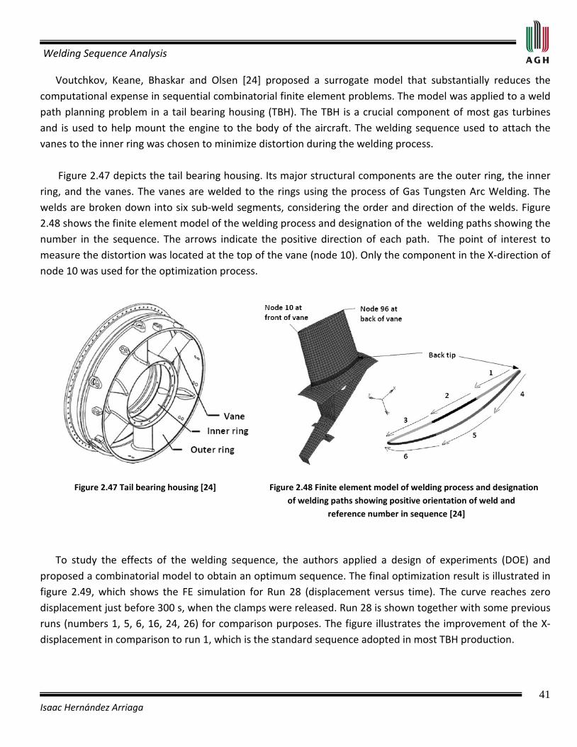
Welding Sequence Analysis
41 Isaac Hernández Arriaga
Voutchkov, Keane, Bhaskar and Olsen [24] proposed a surrogate model that substantially reduces the computational expense in sequential combinatorial finite element problems. The model was applied to a weld path planning problem in a tail bearing housing (TBH). The TBH is a crucial component of most gas turbines and is used to help mount the engine to the body of the aircraft. The welding sequence used to attach the vanes to the inner ring was chosen to minimize distortion during the welding process. Figure 2.47 depicts the tail bearing housing. Its major structural components are the outer ring, the inner ring, and the vanes. The vanes are welded to the rings using the process of Gas Tungsten Arc Welding. The welds are broken down into six sub-weld segments, considering the order and direction of the welds. Figure 2.48 shows the finite element model of the welding process and designation of the welding paths showing the number in the sequence. The arrows indicate the positive direction of each path. The point of interest to measure the distortion was located at the top of the vane (node 10). Only the component in the X-direction of node 10 was used for the optimization process.
Figure 2.47 Tail bearing housing [24] Figure 2.48 Finite element model of welding process and designation of welding paths showing positive orientation of weld and reference number in sequence [24]
To study the effects of the welding sequence, the authors applied a design of experiments (DOE) and proposed a combinatorial model to obtain an optimum sequence. The final optimization result is illustrated in figure 2.49, which shows the FE simulation for Run 28 (displacement versus time). The curve reaches zero displacement just before 300 s, when the clamps were released. Run 28 is shown together with some previous runs (numbers 1, 5, 6, 16, 24, 26) for comparison purposes. The figure illustrates the improvement of the X-displacement in comparison to run 1, which is the standard sequence adopted in most TBH production.
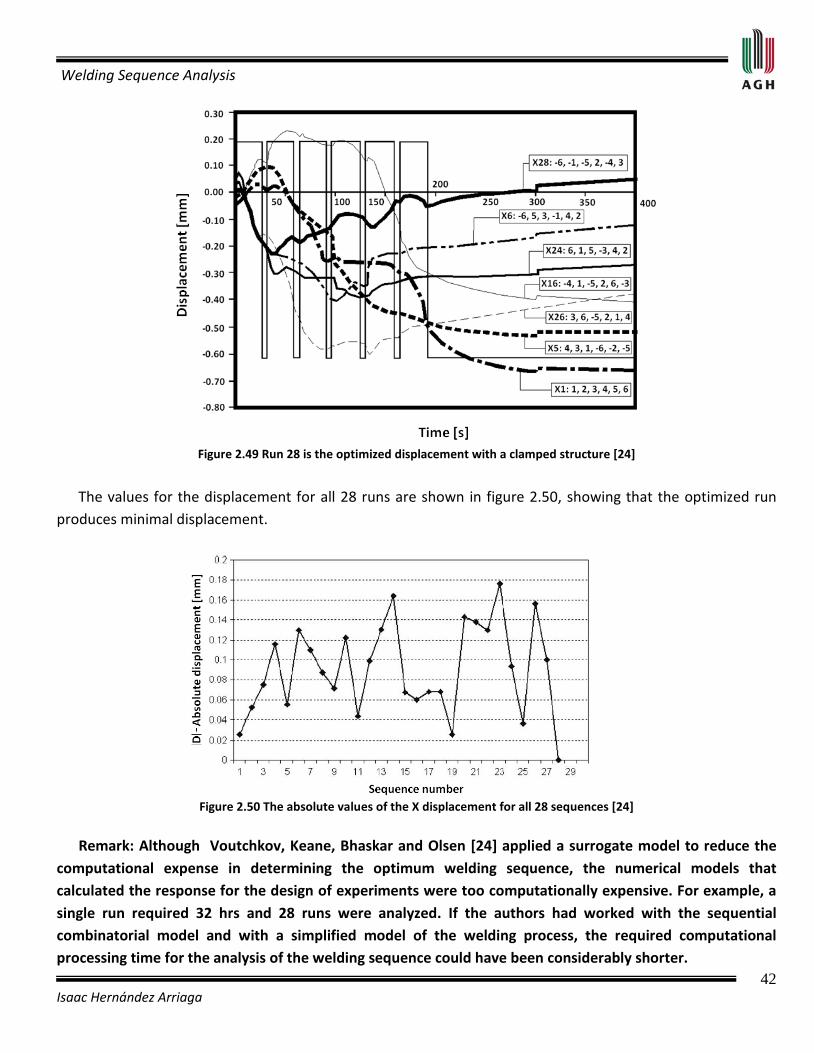
Welding Sequence Analysis
42 Isaac Hernández Arriaga
Figure 2.49 Run 28 is the optimized displacement with a clamped structure [24]
The values for the displacement for all 28 runs are shown in figure 2.50, showing that the optimized run produces minimal displacement.
Figure 2.50 The absolute values of the X displacement for all 28 sequences [24]
Remark: Although Voutchkov, Keane, Bhaskar and Olsen [24] applied a surrogate model to reduce the computational expense in determining the optimum welding sequence, the numerical models that calculated the response for the design of experiments were too computationally expensive. For example, a single run required 32 hrs and 28 runs were analyzed. If the authors had worked with the sequential combinatorial model and with a simplified model of the welding process, the required computational processing time for the analysis of the welding sequence could have been considerably shorter.
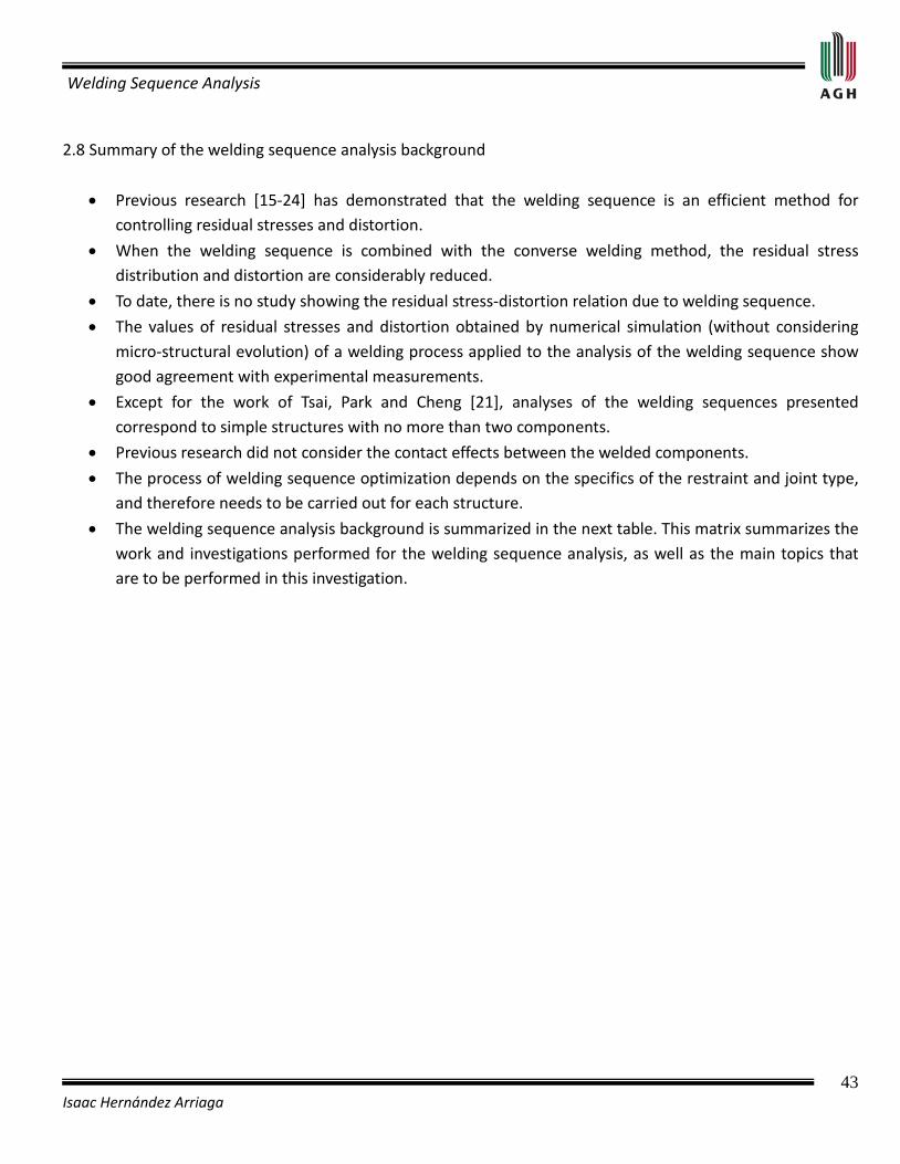
Welding Sequence Analysis
43 Isaac Hernández Arriaga
2.8 Summary of the welding sequence analysis background
• Previous research [15-24] has demonstrated that the welding sequence is an efficient method for controlling residual stresses and distortion.
• When the welding sequence is combined with the converse welding method, the residual stress distribution and distortion are considerably reduced.
• To date, there is no study showing the residual stress-distortion relation due to welding sequence.
• The values of residual stresses and distortion obtained by numerical simulation (without considering micro-structural evolution) of a welding process applied to the analysis of the welding sequence show good agreement with experimental measurements.
• Except for the work of Tsai, Park and Cheng [21], analyses of the welding sequences presented correspond to simple structures with no more than two components.
• Previous research did not consider the contact effects between the welded components.
• The process of welding sequence optimization depends on the specifics of the restraint and joint type, and therefore needs to be carried out for each structure.
• The welding sequence analysis background is summarized in the next table. This matrix summarizes the work and investigations performed for the welding sequence analysis, as well as the main topics that are to be performed in this investigation.

Welding sequence analysis
44 Isaac Hernández Arriaga
2.9 Matrix of the welding sequence analysis background Article
Numerical model
Welding sequence Joint type Material Analized parameters
Dimension of analysis
Welding process
Remarks
Effect of welding sequence on residual stresses. Teng, Peng, Chang and Tseng, 2003.
Thermo‐elastic‐plastic(weld bead thermal cycle is simulated)
Progressive welding , backstep welding, symmetric welding, and jump welding
Single‐pass and multi–pass butt‐ weld joints and circular patch weld joints
SAE 1020steel
Residual stresses In the plane GMAW The methodology is applicable only to simple structures; in addition, the welding direction is not considered in the numerical simulation. No experimental tests were performed to compare the numerical results of the different welding sequences.
Influence of a welding sequence on the welding residual stress of a thick plate. Ji, Fang and Liu, 2005.
Thermo‐elastic‐plastic
8 welding sequences combined with converse welding method
Double V‐groove with multi‐layer weld joints
Martensite stainless steel
1Cr12NiWMoNb
Residual stresses I In the plane
GMAW An important disadvantage is the computational cost resulting from the processing time required to simulate the welding process. This is because the effects of phase transformation and the type of source of heat used were considered.
Three‐dimensional thermal response of thick plate weldments: effect of layer‐wise and piece‐wise welding. Nami, Kadivar and Jafarpur, 2004.
Thermo‐visco‐plastic
Piece‐wise welding (block sequences)
V‐groove with single‐pass butt‐ weld joints
Mild steel Residual stressesand distortion
In the space There is no information
The authors did not present a study of the effects of the welding sequence on the relationship between distortion and residual stresses. Furthermore, the proposed methodology is expensive with respect to the time of processing to simulate the welding process due to the consideration of visco‐plastic effects.
Residual stress distribution depending on welding sequence in multi‐pass welded joints with X‐ shaped groove. Mochizuki and Hayashi, 2000.
Thermal‐elastic‐plastic
6 welding sequences for a multi‐pass welded pipe joints
Multi‐pass welded joints with X‐shaped grove
Austeniticstainless steel
Residual stresses In the plane GTAW The analytical method proposed to determine the residual stresses through‐thickness is only applicable to multi‐pass, welded pipe joints. Therefore, the method is not valid for pipe joints of small diameter. The method presented has a good qualitative correlation with the experimental and numerical data. However, there was not a good correlation quantitatively.
Residual stress reduction and fatigue strength improvement by controlling welding pass sequence. Mochizuki, Hattori and Nakakado, 2000.
Thermo‐elastic‐plastic
2 welding sequence for multi‐pass fillet weld joints
Multi‐pass fillet weld joints
Carbon steelJIS SS400
Residual stresses In the plane CO2 Gas Arc
The methodology is valid for simple fillet joints only. Two very similar welding sequences were used where only two weld beads were changed.
Welding distortion of a thin‐plate panel structure. Tsai, Park and Cheng, 1999.
Inherent shrinkage method
4 welding sequences for single pass fillet weld joints
Single‐pass fillet weld joints
Aluminum5456‐H116
Distortion In the space GMAW
The welding in the perpendicular direction and between the T‐stiffeners was not considered. Therefore, the proposed method to optimize the welding sequence is limited to rigid, co‐lineal joints.
Application of welding simulation for chassis components within the development of manufacturing methods. Hackmair, Werner and Pönisch, 2003.
Thermo‐elastic‐plastic
2 welding sequence for single ‐pass fillet weld joints
Single‐pass fillet weld joints
Aluminum alloy 6060 T6
Temperature distribution and
distortion
In the space MIG
The gap effects between two separate extrusions are not considered. For this reason, the quantitative results show a considerable difference. The proposed methodology is only applied to simple joints. Therefore, a local/global method is required for more complex structures, which implies a high computational cost (time of processing).
Welding distortion minimization for an aluminum alloy extruded beam structure using a 2D model. Bart, Nnaji, Deepak and Kim,2004.
Pre‐estimated angular shrinkages
4 welding sequences for single–pass fillet weld joints
Single‐pass fillet weld joints
Aluminum alloy
Distortion In the plane There is no information
The contact effect between the beams was not considered. Also, a study of the effects of the welding sequence on the distribution of the residual stresses was not performed. This study is of great importance because it shows that in constrained structures the residual stress has a critical effect.
Optimizing welding sequence with genetic algorithm. Kadivar, Jafarpur and Baradaran. 2000.
ThermoelastIc‐ viscoplastic
Continuous sequence, optimum sequences and 4 random sequences
Circular patch weld joints
Stainless304 L
Distortion In the plane There is no information
The applied genetic algorithm method is valid for simple joints only. Therefore, the uses of other genetic algorithms are required for complex joints. In addition, experimental tests to check the optimum sequence obtained by genetic algorithm were not performed.
Weld sequence optimization: the use of surrogate models for solving sequential combinatorial problems. Voutchkov, Keane, Bhaskar and Olsen, 2005.
Thermo‐elastic‐plastic
27 Random welding sequence determined by DOE and the optimum welding sequence
Single‐pass fillet weld joints
Inconel 718
Distortion In the space TIG Although a surrogate model that can be used to reduce the computational expense to determine the optimum welding sequence was presented, the numeric models used to measure the response for the design of experiments were too expensive with respect to the required computational processing time
Welding sequence analysis Hernández A. I. Research work 2009
Thermo‐elastic‐plastic (weld bead thermal cycle is simulated)
36 welding sequences base on empirics rules
Single‐pass butt‐weld joints and single‐pass fillet weld joints
ASTM A36 Steel(Poland≈St3s)
Residual stresses,distortion
And a relationship between both parameters
In the plane and in the space
SMAWand
GMAW‐MAG
Formulation of the welding sequences most appropriates to reduce residual stress, distortion or a relationship between both parameters for symmetrical structures in the plane and in the space. Possible generalization of the example
Welding Sequence Analysis
45 Isaac Hernández Arriaga
CHAPTER III
PROPOSAL OF A NUMERICAL SIMULATION OF THE WELDING PROCESS
AND A NUMERICAL SIMULATION OF THE WELDING
SEQUENCE IN AN L-TYPE STRUCTURE 3.1 Introduction This chapter presents a finite element simulation of the welding processes with the objective of defining the initial and boundary conditions and studying the effects of the welding sequence on the residual stress distribution and distortion in symmetrical structures in 2 and 3 dimensions. Although the analysis focuses on symmetrical structures, the proposed numerical model is applicable to asymmetrical structures. The proposed sequentially-coupled thermo-mechanical analysis involves two steps: a transient heat transfer analysis is performed followed by a thermal elastic plastic analysis. This numerical simulation is performed in an I-type specimen subject to tension and validated with experimental data [25] to check the accuracy of the proposed numerical model. The end of this chapter presents a numerical simulation of the welding sequence in an L-type structure to test whether the proposed numerical model can simulate the effects of the welding sequence on residual stresses and distortion, with respective adaptations. 3.2 Heat transfer in welding The temperature distribution in a weldment is mainly determined by the total heat input, the preheat temperature, the welding process, and the type and geometry of joint. The latent heat released during phase transformation only marginally affects the temperature distribution. The temperature field in the molten pool is in general assumed to be governed by the same equation as is applied to the solid metal. In most metallurgical and structural studies of welding, the energy transfer from the electrode to the weld metal is represented either by a surface heat source or by momentarily deposited energy that gives the weld metal an initial temperature distribution.
Welding Sequence Analysis
46 Isaac Hernández Arriaga
In general the temperature field should be taken as thermodynamically coupled to the mechanical field. The governing equation of the heat flow follows the first law of thermodynamics (conservation of energy). This law states that the rate of change of internal energy and conduction must be in equilibrium with the heat production and the power of elastic and viscoplastic straining and , respectively [26]:
(1)
The parameter takes on the value of 1 if all inelastic dissipation is converted into heat. The mechanical coupling terms in (1) are in most cases not considered because their influence on the temperature field is very small [27]. It is therefore possible to divide the thermo-mechanical analysis of a welding process into two main parts: the analysis of the temperature field and subsequent analysis of the mechanical fields. 3.2.1 Analytical solution for the temperature field Neglecting the mechanical coupling terms in Eq. (1), the energy equation becomes [27]:
(2)
Equations (1) and (2) are statements of the First Law of Thermodynamics [28]. Fourier’s law of heat transfer [28] defines a relationship between the heat flux and the gradient of the temperature field . For an isotropic material this relationship is the Fourier heat conduction Law: (3) Where is the thermal conductivity for the material. Equation (2) and (3) give
(4)
In Cartesian coordinates x, y, z, equation (4) becomes
(5)
Where: is the thermal conductivity in the , and directions, respectively, is the
temperature, is the density, is the specific heat and is time. Equation (5) becomes nonlinear if material properties and C are a function of temperature. The first term is conduction of heat through the
material. The second term is the source of heat generation. The last term is the rate of change of internal energy.
Welding Sequence Analysis
47 Isaac Hernández Arriaga
There are only three terms in the heat equation (with zero velocity) that can be “manipulated” in addition to the associated boundary conditions of either prescribed flux or prescribed temperature type. Therefore any model of a weld heat source based on the heat equation must specify something about one or more terms in this heat equation or its BCs. Suppose that a heat source is moving at a constant speed in the positive direction. We can define an Eulerian (moving) frame with origin at the center of the source (i.e., a welding arc), and coordinates . The transformation from to is given by [29]: (6) Where: is time. Noting that the material time derivate in equation (4) becomes:
(7)
We obtain the equation of conservation of energy in the Eulerian frame:
(8)
Here, represents the time derivate of temperature at a point fixed with respect to the heat source. In steady state, this derivate is zero, and so equation (8) becomes:
(9)
When and are constant, equation (9) can be solved more easily by applying the transformation:
(10) Substituting equation (10) into (9), we have:
(11)
(12)
Equation (12) is symmetric positive definite. After properly transforming the boundary conditions from
to function, it is easy to solve this equation with standard Lagrangian FEM code that
Welding Sequence Analysis
48 Isaac Hernández Arriaga
contains a solver for positive definite symmetric matrix. Equation (12) applies only to linear systems (i.e., is independent of ) because of equation (11). 3.2.2 Thermal initial and boundary Conditions The solution of the heat conduction equation (4), involves a number of arbitrary constants to be determined by specified initial and boundary conditions. These conditions are necessary to translate the real physical conditions into mathematical expressions [28]. Initial conditions are required only when dealing with transient heat transfer problems (in which the temperature field changes with time). The common initial condition in a material can be expressed mathematically as [28]: (13) On the boundary of the domain either the essential (prescribed temperature) or natural (prescribed flux) boundary conditions must be satisfied. Five common types of boundary conditions are [28]: Essential boundary condition: a) Prescribed surface temperature, it is often necessary to prescribe a surface temperature for a structure. The mathematically expression takes the form: (14) Natural boundary condition b) Prescribed heat input, many structures, particularly in the case of welding, have the boundary surface exposed to a heat source or sink. Let denote the outward normal to the surface at the point , then the mathematical formulation for the heat input across a solid boundary is:
(15)
(c) Perfectly insulated surface, by definition, a perfectly insulated surface is one across which there is no heat flux. Equation (15) becomes:
(16)
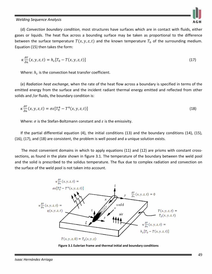
Welding Sequence Analysis
49 Isaac Hernández Arriaga
(d) Convection boundary condition, most structures have surfaces which are in contact with fluids, either gases or liquids. The heat flux across a bounding surface may be taken as proportional to the difference between the surface temperature and the known temperature of the surrounding medium. Equation (15) then takes the form:
(17)
Where: is the convection heat transfer coefficient. (e) Radiation heat exchange, when the rate of the heat flow across a boundary is specified in terms of the emitted energy from the surface and the incident radiant thermal energy emitted and reflected from other solids and /or fluids, the boundary condition is:
(18)
Where: is the Stefan-Boltzmann constant and is the emissivity. If the partial differential equation (4), the initial conditions (13) and the boundary conditions (14), (15), (16), (17), and (18) are consistent, the problem is well posed and a unique solution exists. The most convenient domains in which to apply equations (11) and (12) are prisms with constant cross-sections, as found in the plate shown in figure 3.1. The temperature of the boundary between the weld pool and the solid is prescribed to the solidus temperature. The flux due to complex radiation and convection on the surface of the weld pool is not taken into account.
Figure 3.1 Eulerian frame and thermal initial and boundary conditions
Welding Sequence Analysis
50 Isaac Hernández Arriaga
3.3 Thermal elastic plastic stress analysis in welding In the mechanical analysis, the temperature history obtained from the thermal analysis is introduced as a thermal loading. Thermal strains and stresses can be calculated at each time increment, and the final state of residual stresses will be accumulated by thermal strains and stresses. Residual stresses in each temperature increment are added to those at nodal points to update the behavior of the model before the next temperature increment. 3.3.1 Mechanical equations Three basic sets of equation relating to the mechanical model, the equilibrium and compatibility equations and the constitutive equations for thermal elastic plastic material, are considered as follows [1]: , 0ij j ifσ + = (19)
Where: if is the sum of the body force and ijσ is the Cauchy stress tensor. To ensure that the body
remains continuous during the deformation, the compatibility equations must be satisfied [2]. , , , , 0ij kl kl ij ik jl jl ikε ε ε ε+ − − = (20)
The thermal elastic plastic material model will be derived assuming isotropic material, von Mises yield criterion and the associated flow rule and linear isotropic hardening. Thermal and mechanical properties of the selected material are a function of temperature. The micro-structural evolution is not considered. The initial assumption is that the total strain increment can be decomposed as (valid for small strains and rotations) [1]:
e p
ij ij ij ijd d d d θε ε ε ε= + + (21)
Stress-strain relations can be written as
2
2
31 123 1 2 31
3
ij kl klij ij kk ij ij kk
VM
Gs s dEd d Gd K dT dKHv KG
εσ δ ε ε δ α σ
σ
= + − − + − +
11
1 13 3
ijij
VM
fs dTs TdGH HGG G
σ
∂ ∂ + − +
+ +
(22)
Welding Sequence Analysis
51 Isaac Hernández Arriaga
The variation of the material properties dG and dK in equation (22) is due to the temperature only [2]. These equations are treated in more detail in appendix No.1 3.3.2 Mechanical initial and boundary conditions Initial conditions are necessary only when the analysis is transient [30] and therefore will not be specified in the static mechanical analysis described here. In a mechanical problem, the boundary conditions can be specified in three different ways: Type I: Specification of the primary variable (degree of freedom). Type II: Specification of variables related to the derivative of the primary variable. Type III: Specification of a linear combination of the primary variable and its derivate. The primary variables are the displacement components. When Type I boundary conditions are used, the displacement constraints are specified along a segment of the boundary. Rotations at the boundary are Type II because rotations are related to the derivatives of the displacement components. 3.4 Finite element solution of the welding We have selected finite element modeling has over existing alternatives for detailed analysis (finite difference and boundary element) for its capability for nonlinear analysis in complex geometries. Finite element is also most compatible with modern CAD/CAM software systems. For thermal analysis alone, a strong argument can be made in favor of finite difference methods. However, for thermal elastic plastic analysis finite element analysis holds an advantage. The boundary element method is not well developed for nonlinear analysis. Briefly, these considerations led to the choice of FEA as the most effective numerical method for developing a complete analysis capability for computer modeling or simulation of welds. Finite element is a generalized Rayleigh-Ritz method, which uses interpolation to express the variables in terms of its values in a finite number of nodes. 3.4.1 Finite element solution of heat transfer in welding The finite element method FEM usually imposes a piece-wise polynomial approximation of the temperature field within each element [29]:
(23)
Welding Sequence Analysis
52 Isaac Hernández Arriaga
Where: are basis functions dependent only on the type element and its size and shape. Physically is the value of the temperature at node at time .
(24)
Where: is abbreviated to . The next question is how to evaluate ? Garlekin´s FEM is among the most convenient and general of the methods available for this purpose. If equation (23) is substituted into equation (4), a residual or error term must be added. Otherwise equation (23) would be the exact solution. Indeed when equation (23) is the exact solution, the error in the FEM solution is zero. Garlekin´s FEM method requires [29]:
(25)
Mathematically is the residual from equation (4); in equation (25) is a test function and the terms in equation (23) are the trial functions. Since there are nodes, equation (25) creates a set of ordinary differential equations which are integrated to form a set of algebraic equations for each time step: (26) This set of equations is solved for the nodal temperatures at the end of the time step. Usually some form of Newton-Raphson method together with a Gaussian elimination and back substitution would be employed. 3.4.2 Finite element solution of the thermal elastic plastic stress analysis in welding In welding, no external force is applied to the welded structure. Thermal loads are the only source of residual stress and distortion [1-3]. Therefore, the principle of virtual work in this case, without mechanical loading, is written as [26]:
0ij ijV
d d dVδ ε σ =∫ (27)
Where: ijdδ ε is the variation in the strain increment ijdε . The stress increment ijdσ is given in equation
(22).
Welding Sequence Analysis
53 Isaac Hernández Arriaga
In matrix notation, the thermal elastic plastic constitutive equation (eqn. 22) becomes [26]:
{ } { } { } { }epd D d C s M dTσ ε α = − − (28)
Where: epD is the elastic plastic stiffness matrix, { }C s and { }M dTα are terms related with the
distortion and volume change due to the temperature. The virtual work equation (27) is now written as:
{ } { } 0T
V
d d dVδ ε σ =∫ (29)
Where: is the volume of the body to be analyzed and is the transpose of . The strain-displacement for three-dimensional problem can be written in matrix form as [26]:
{ } { }
0 0
0 0
0 0
0
0
0
x
y
zd du
y x
z y
z x
ε
∂ ∂
∂ ∂
∂ ∂
= ∂ ∂ ∂ ∂ ∂ ∂ ∂ ∂ ∂ ∂ ∂ ∂
(30)
In the finite element solution, the increments in the displacements for each element are approximated as [30]:
{ } ( ){ }1
, ,n
ii
du N x y z U=
= ∆∑ (31)
Where: n is the number of nodal points for each element, ( , , )iN x y z are the shape functions and { }U∆are element nodal increments.

Welding Sequence Analysis
54 Isaac Hernández Arriaga
Substituting equation (31) into equation (32) produces the following expresion:
{ } [ ]{ }d B Uε = ∆ (32)
Where: [ ] [ ] ( )1
, ,n
ii
B N x y z=
= ∂ ∑ is the strain-displacement matrix for each element.
Using equation (31) and equation (32) yields:
{ } { } [ ]T T Td U Bδ ε δ= ∆ (33)
Substituting equations (27), (28) and (32) into equation (29) yields
{ } [ ] [ ][ ] { } [ ] { } [ ] { } 0T T T T
V V V
U B D B dV U C B s dV M B d dVθδ ε
∆ ∆ − − = ∫ ∫ ∫ (34)
The vectors { }Uδ ∆ and { }U∆ are not included in the integrals because they are not a function of the
coordinates. Equation (34) must be valid for any admissible virtual nodal increase { }Uδ ∆ of equilibrium
configuration. Therefore, equation (34) becomes:
{ } [ ]{ } { }{ } 0TU K U F∆ ∆ − = (35)
Now, the expressions inside the braces must be zero, therefore:
[ ]{ } { }K U F∆ = (36)
Where:[ ]K is the global stiffness matrix for the assembly of elements and is formed as a sum of the
element stiffness matrices and is the global load vector, formed as the sum of the element load vectors . The stiffness matrix for each element is:
[ ] [ ] [ ]e
T epe
V
K B D B dV = ∫ (37)

Welding Sequence Analysis
55 Isaac Hernández Arriaga
And the element load vector is:
{ } [ ] { } [ ] { }e e
T Te
V V
F M B dT dV C B s dVα= +∫ ∫ (38)
Equation (36) is solved for each load (time) increment. The stiffness matrix is in most cases updated at every load increment. It is often advantageous to use the elastic stiffness matrix only, computed at the beginning of each time step in a modified Newton-Raphson approach. The non-linearities are compensated for by equilibrium iterations and the stress increment during each load (time) increment are often calculated using the subincrement technique. The matrix element in is typically integrated with Gauss quadrature. The reader is referred to Appendix 1 for detailed treatment of this set of equations. 3.5 Geometric configuration of I-type specimen subject to tension The finite element welding simulation is performed with a commercial code on an I-type specimen subject to tension. This geometry is selected due to the availability of experimental data [25]. A static linear model was used with a shrinkage force (transverse to weld bead) applied in the boundary between the weld metal and the base metal to simulate the effects of the welding process. In the present work, a thermo-mechanical analysis that includes plastic behavior and temperature distribution will be developed. The I-type specimen subject to tension consists of a central bar and two lateral bars (restraining members). When the weld metal solidifies and shrinks, tensile residual stresses are induced in the central bar, while in the lateral bars compression residual stresses are induced. This is due to the balance conditions and geometry [3]. Figure 3.2 depicts the geometric configuration of an I-type specimen subject to tension.
Figure 3.2 Geometric configuration of I-type specimen subject to tension (mm) [25]

Welding Sequence Analysis
56 Isaac Hernández Arriaga
3.6 Material selection for the I-type specimen subject to tension The material selected is ASTM A36 steel because of its common use in the welding industry. The chemical composition of ASTM A36 is shown in table 3.1.
Chemical composition of ASTM A36 (%)
C Mn P S Si Fe
0.21-0.29 1.0 0.04 0.05 0.28 98.0 min
Table 3.1 Chemical composition of ASTM A36 carbon steel [33]
3.7 Temperature-dependent thermal and mechanical properties of ASTM A36 Temperatures vary widely within the welded part. Therefore, thermal and mechanical properties of welded materials vary significantly [34]. The thermal and mechanical properties of ASTM A36 due to temperature are shown in figure 3.3.
Figure 3.3 Thermal and mechanical properties of ASTM A36 as a function of temperature [34]
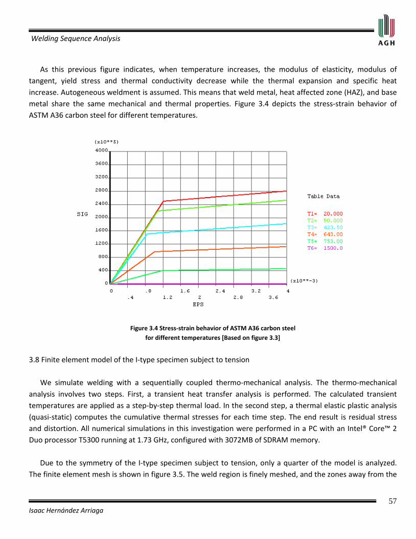
Welding Sequence Analysis
57 Isaac Hernández Arriaga
As this previous figure indicates, when temperature increases, the modulus of elasticity, modulus of tangent, yield stress and thermal conductivity decrease while the thermal expansion and specific heat increase. Autogeneous weldment is assumed. This means that weld metal, heat affected zone (HAZ), and base metal share the same mechanical and thermal properties. Figure 3.4 depicts the stress-strain behavior of ASTM A36 carbon steel for different temperatures.
Figure 3.4 Stress-strain behavior of ASTM A36 carbon steel for different temperatures [Based on figure 3.3]
3.8 Finite element model of the I-type specimen subject to tension We simulate welding with a sequentially coupled thermo-mechanical analysis. The thermo-mechanical analysis involves two steps. First, a transient heat transfer analysis is performed. The calculated transient temperatures are applied as a step-by-step thermal load. In the second step, a thermal elastic plastic analysis (quasi-static) computes the cumulative thermal stresses for each time step. The end result is residual stress and distortion. All numerical simulations in this investigation were performed in a PC with an Intel® Core™ 2 Duo processor T5300 running at 1.73 GHz, configured with 3072MB of SDRAM memory. Due to the symmetry of the I-type specimen subject to tension, only a quarter of the model is analyzed. The finite element mesh is shown in figure 3.5. The weld region is finely meshed, and the zones away from the

Welding Sequence Analysis
58 Isaac Hernández Arriaga
weld bead have a relatively coarse mesh. This guarantees accuracy while reducing the calculation time. The numerical model is divided into 1536 hexahedral elements and 2420 nodes.
Figure 3.5 Finite element mesh of the I-type specimen subject to tension
3.8.1 Definition and justification of the applied finite elements To perform the thermal analysis, it is necessary to select an element type that is able to simulate:
• A transient thermal analysis.
• The weld thermal cycle [figure 3.6, page 60], which determines the temperature as a function of the time in the weld bead (i.e., all elements belonging to the weld bead).
• The conduction phenomenon that occurs in the base metal as primary mode of heat transfer.
• The phenomenon of heat loss by convection to the surrounding in the base metal, moreover it is required to calculate the rate of change of internal energy.
• Activation and de-activation of the weld bead elements. To perform the structural analysis, it is necessary to select an element type that is able to simulate:
• Homogeneous and isotropic material.
• Elastic-plastic material´s behavior following the von Mises yield criterion and the associated flow rule with linear isotropic hardening by strain.
• Small strains.
• Activation and de-activation of the weld bead elements.

Welding Sequence Analysis
59 Isaac Hernández Arriaga
Furthermore, it is necessary to select an element type that with the temperature in each node and the thermal expansion coefficient, it can couple these data with the structural unitary strain. ANSYS offers a broad variety of elements for the analysis of two and three-dimensional thermal and structural problems. In table 1 and 2 some common element used by ANSYS are presented. In general, all elements have the same characteristics (degree of freedom, input data, and output data), only there are two main differences: 1) the order of elements: higher order elements achieve better results and greater accuracy, however, these elements require more computational time. This time requirement is because numerical integration of elemental matrices is more involved, also, these elements are well suited to model problems with curved boundaries. 2) The shape of element: quadrilateral and brick element present better meshing control than triangular and tetrahedral elements. For these two reasons, PLANE55 and SOLID70 elements are selected for two and three dimensional thermal analysis, respectively. Both elements have a single degree of freedom, temperature and isotropic material properties. These elements alloy simulate these thermal conditions mentioned early without complications, which is necessary to introduce the thermal conductivity and specific heat as a function of temperature [Fig 3.3, page 56], the convective heat transfer coefficient (natural convection), this coefficient is considered constant and is equal to 10 W/m2 ºC. Heat loss by convection is a boundary condition and is applied only to surfaces in contact with the surrounding. It is also required to introduce the temperature of the surrounding, which is a boundary condition (20°C) and the initial condition of base metal, which is considered as the ambient temperature (20°C). The elements PLANE42 and SOLID45 are selected for two and three dimensional structural analysis, respectively. PLANE 42 and SOLID45 elements have two and three degrees of freedom at each node, respectively: translation in the nodal directions and isotropic material properties. Both elements couple the temperature with strain, for this reason it is necessary to introduce the thermal expansion coefficient, elasticity modulus, tangent modulus, yield stress and Poisson´s ratio dependent on temperature as shown in figure 3.3 [page 56]. Finally, to transfer the thermal loads obtained in the transient thermal analysis to the structural analysis, the concept of body load is used through load step. PLANE 42 and SOLID45 elements have this capability because the temperatures may be input as body loads at the nodes. The elements PLANE42 and SOLID55, and SOLID70 and SOLID45 are equivalent to perform coupled thermo-mechanical analysis. Definition and justification of the applied finite elements are treated in more detail in appendix No.2. 3.8.2 Thermal initial and boundary conditions As mentioned early, these conditions are necessary to express the real physical conditions into mathematical expressions. For all numerical simulation developed in the present research, the initial and boundary conditions are equal, unless otherwise noted.

Welding Sequence Analysis
60 Isaac Hernández Arriaga
a) Initial condition: Because the thermal model consists of a transient heat transfer analysis, it is required an initial condition of the base metal, which is considered as the surrounding temperature ( =20°C). b) Boundary conditions (see figure 3.5, page 58): Symmetrical plane: Plane y-z in x=0; and plane x-z in y=0; Surfaces in contact with the surrounding except surfaces belonging to weld metal:
Nodes belonging to weld metal:
Prescribed heat input: heat loading is simulated via weld thermal cycle curves shown in figure 3.6. The input heat is applied to all surfaces between the weld metal and the base metal.
Figure 3.6 Weld thermal cycle of ASTM A36 carbon steel [34-35]
Welding Sequence Analysis
61 Isaac Hernández Arriaga
3.8.3 Mechanical boundary condition In the structural analysis, the parameters and are the displacements in the X, Y, and Z-direction, respectively. , , and are the strain in the X, Y, and Z-direction, respectively. , , and are the rotation with respect to X, Y, and Z axis, respectively. a) Symmetrical plane (see figure 3.5, page 58): Plane y-z in x=0;
and
; ← due to Poisson´s ratio and pure tension Plane x-z in y=0;
and
← due to Poisson´s ratio and pure tension b) Surfaces in contact with the surrounding (see figure 3.5, page 58): The normal stresses to the surfaces in contact with the surrounding and the shear stresses are zero (i.e., in the plane x-z in y=50.8 mm, ). c) For all surfaces including the surfaces belonging to symmetrical planes, the shearing strain is zero due to pure tension. 3.8.4 Body load Body loads can be generated internally or externally as the result of physical fields acting volumetrically on the body. Gravity, inertial loads, and temperature changes represent body loads in a mechanical problem [26]. In the present research, we use the concept of body load to transfer the transient thermal loads to the static

Welding Sequence Analysis
62 Isaac Hernández Arriaga
structural analysis. The use of load steps is necessary to calculate the response of the structure to temperatures obtained from transient thermal analysis at specific points in time. 3.8.5. Solution to the finite element model After completing the finite element mesh and specifying the loading conditions (boundary, initial and body loads), the solution can be initiated. In the transient thermal analysis, the time to complete the weld bead is 6 seconds, and the time to return to its initial temperature is 1200 seconds [25]. The thermal elastic plastic analysis requires 15 load steps to complete the weld thermal cycles (1, 3, 10, 20, 35, 50, 75, 100, 200, 300, 400, 600, 750, and 1200 seconds). All the computational analysis was done using ANSYS®. 3.9 Points of interest in the finite element model of the I-type specimen subject to tension Experimental data was taken from an I-type specimen subject to tension [25]. Residual stresses in the X-direction were obtained in two points of interest. The same points (Figure 3.7) are selected on the finite element model to carry out a quantitative comparison
Figure 3.7 Localization of the points of interest on finite element model
3.10 Residual stresses in the I-type specimen subject to tension obtained in the numerical simulation The results of interest are the residual stresses in the two selected points. Table 3.2 depicts the values of the residual stresses in the X-direction obtained in the numerical simulation.
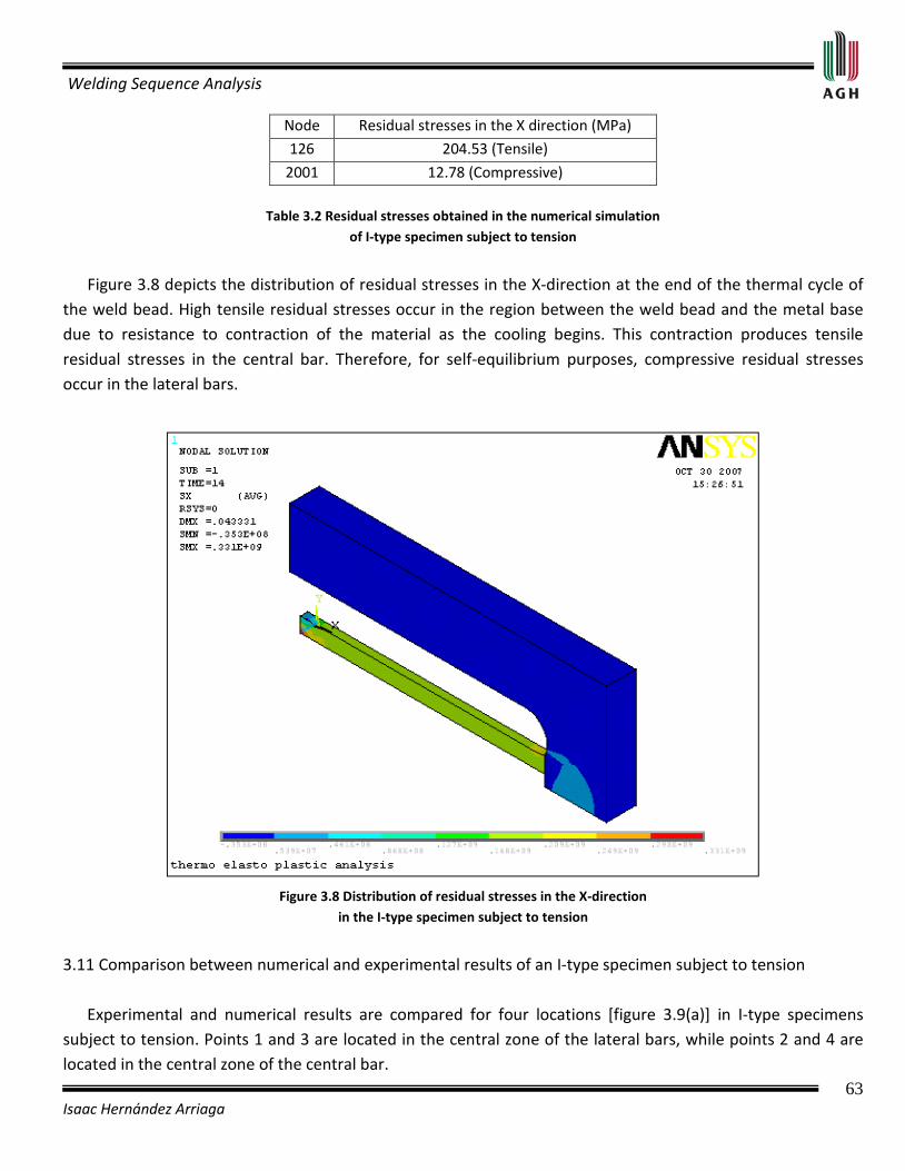
Welding Sequence Analysis
63 Isaac Hernández Arriaga
Node Residual stresses in the X direction (MPa)
126 204.53 (Tensile)
2001 12.78 (Compressive)
Table 3.2 Residual stresses obtained in the numerical simulation of I-type specimen subject to tension
Figure 3.8 depicts the distribution of residual stresses in the X-direction at the end of the thermal cycle of the weld bead. High tensile residual stresses occur in the region between the weld bead and the metal base due to resistance to contraction of the material as the cooling begins. This contraction produces tensile residual stresses in the central bar. Therefore, for self-equilibrium purposes, compressive residual stresses occur in the lateral bars.
Figure 3.8 Distribution of residual stresses in the X-direction
in the I-type specimen subject to tension
3.11 Comparison between numerical and experimental results of an I-type specimen subject to tension Experimental and numerical results are compared for four locations [figure 3.9(a)] in I-type specimens subject to tension. Points 1 and 3 are located in the central zone of the lateral bars, while points 2 and 4 are located in the central zone of the central bar.
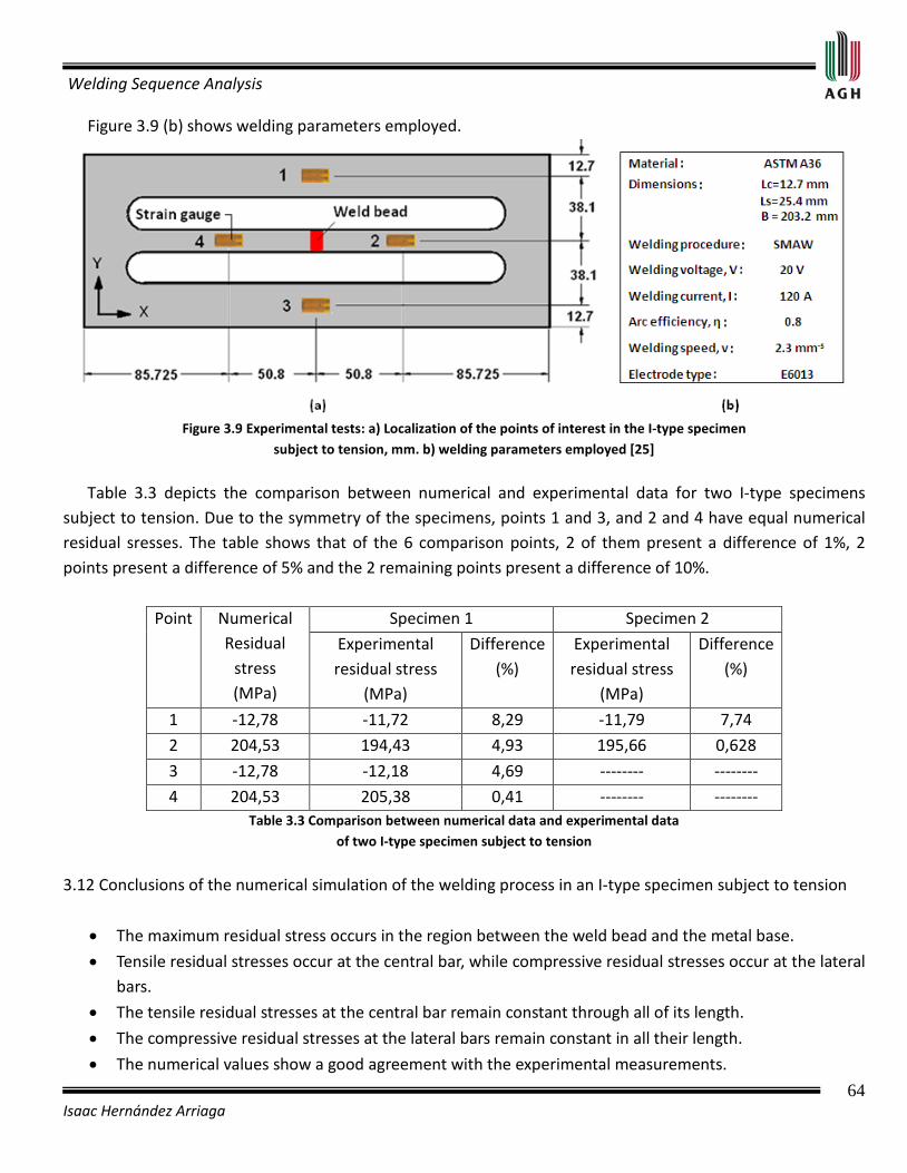
Welding Sequence Analysis
64 Isaac Hernández Arriaga
Figure 3.9 (b) shows welding parameters employed.
Figure 3.9 Experimental tests: a) Localization of the points of interest in the I-type specimen
subject to tension, mm. b) welding parameters employed [25]
Table 3.3 depicts the comparison between numerical and experimental data for two I-type specimens subject to tension. Due to the symmetry of the specimens, points 1 and 3, and 2 and 4 have equal numerical residual sresses. The table shows that of the 6 comparison points, 2 of them present a difference of 1%, 2 points present a difference of 5% and the 2 remaining points present a difference of 10%.
Point Numerical Residual
stress (MPa)
Specimen 1 Specimen 2
Experimental residual stress
(MPa)
Difference (%)
Experimental residual stress
(MPa)
Difference (%)
1 -12,78 -11,72 8,29 -11,79 7,74
2 204,53 194,43 4,93 195,66 0,628
3 -12,78 -12,18 4,69 -------- --------
4 204,53 205,38 0,41 -------- -------- Table 3.3 Comparison between numerical data and experimental data
of two I-type specimen subject to tension
3.12 Conclusions of the numerical simulation of the welding process in an I-type specimen subject to tension
• The maximum residual stress occurs in the region between the weld bead and the metal base.
• Tensile residual stresses occur at the central bar, while compressive residual stresses occur at the lateral bars.
• The tensile residual stresses at the central bar remain constant through all of its length.
• The compressive residual stresses at the lateral bars remain constant in all their length.
• The numerical values show a good agreement with the experimental measurements.
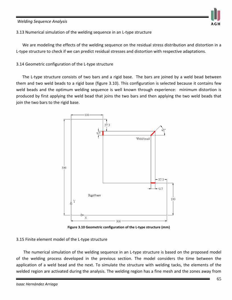
Welding Sequence Analysis
65 Isaac Hernández Arriaga
3.13 Numerical simulation of the welding sequence in an L-type structure We are modeling the effects of the welding sequence on the residual stress distribution and distortion in a L-type structure to check if we can predict residual stresses and distortion with respective adaptations. 3.14 Geometric configuration of the L-type structure The L-type structure consists of two bars and a rigid base. The bars are joined by a weld bead between them and two weld beads to a rigid base (figure 3.10). This configuration is selected because it contains few weld beads and the optimum welding sequence is well known through experience: minimum distortion is produced by first applying the weld bead that joins the two bars and then applying the two weld beads that join the two bars to the rigid base.
Figure 3.10 Geometric configuration of the L-type structure (mm)
3.15 Finite element model of the L-type structure The numerical simulation of the welding sequence in an L-type structure is based on the proposed model of the welding process developed in the previous section. The model considers the time between the application of a weld bead and the next. To simulate the structure with welding tacks, the elements of the welded region are activated during the analysis. The welding region has a fine mesh and the zones away from
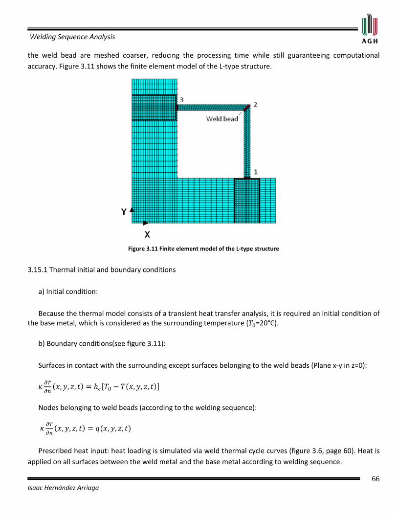
Welding Sequence Analysis
66 Isaac Hernández Arriaga
the weld bead are meshed coarser, reducing the processing time while still guaranteeing computational accuracy. Figure 3.11 shows the finite element model of the L-type structure.
Figure 3.11 Finite element model of the L-type structure
3.15.1 Thermal initial and boundary conditions a) Initial condition: Because the thermal model consists of a transient heat transfer analysis, it is required an initial condition of the base metal, which is considered as the surrounding temperature ( =20°C). b) Boundary conditions(see figure 3.11): Surfaces in contact with the surrounding except surfaces belonging to the weld beads (Plane x-y in z=0):
Nodes belonging to weld beads (according to the welding sequence): Prescribed heat input: heat loading is simulated via weld thermal cycle curves (figure 3.6, page 60). Heat is applied on all surfaces between the weld metal and the base metal according to welding sequence.
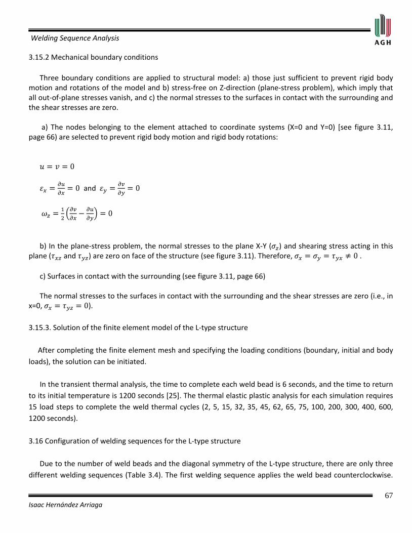
Welding Sequence Analysis
67 Isaac Hernández Arriaga
3.15.2 Mechanical boundary conditions Three boundary conditions are applied to structural model: a) those just sufficient to prevent rigid body motion and rotations of the model and b) stress-free on Z-direction (plane-stress problem), which imply that all out-of-plane stresses vanish, and c) the normal stresses to the surfaces in contact with the surrounding and the shear stresses are zero. a) The nodes belonging to the element attached to coordinate systems (X=0 and Y=0) [see figure 3.11, page 66) are selected to prevent rigid body motion and rigid body rotations:
and
b) In the plane-stress problem, the normal stresses to the plane X-Y ( ) and shearing stress acting in this plane ( and ) are zero on face of the structure (see figure 3.11). Therefore, . c) Surfaces in contact with the surrounding (see figure 3.11, page 66) The normal stresses to the surfaces in contact with the surrounding and the shear stresses are zero (i.e., in x=0, ). 3.15.3. Solution of the finite element model of the L-type structure After completing the finite element mesh and specifying the loading conditions (boundary, initial and body loads), the solution can be initiated. In the transient thermal analysis, the time to complete each weld bead is 6 seconds, and the time to return to its initial temperature is 1200 seconds [25]. The thermal elastic plastic analysis for each simulation requires 15 load steps to complete the weld thermal cycles (2, 5, 15, 32, 35, 45, 62, 65, 75, 100, 200, 300, 400, 600, 1200 seconds). 3.16 Configuration of welding sequences for the L-type structure Due to the number of weld beads and the diagonal symmetry of the L-type structure, there are only three different welding sequences (Table 3.4). The first welding sequence applies the weld bead counterclockwise.
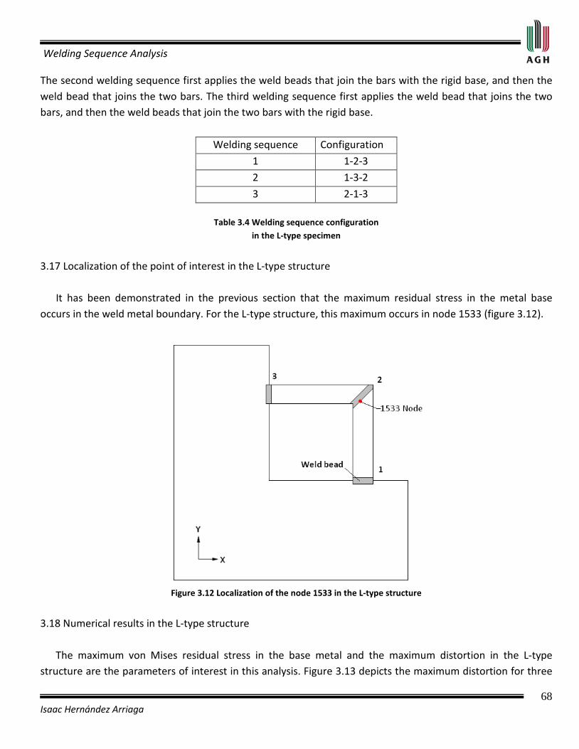
Welding Sequence Analysis
68 Isaac Hernández Arriaga
The second welding sequence first applies the weld beads that join the bars with the rigid base, and then the weld bead that joins the two bars. The third welding sequence first applies the weld bead that joins the two bars, and then the weld beads that join the two bars with the rigid base.
Welding sequence Configuration
1 1-2-3
2 1-3-2
3 2-1-3
Table 3.4 Welding sequence configuration in the L-type specimen
3.17 Localization of the point of interest in the L-type structure It has been demonstrated in the previous section that the maximum residual stress in the metal base occurs in the weld metal boundary. For the L-type structure, this maximum occurs in node 1533 (figure 3.12).
Figure 3.12 Localization of the node 1533 in the L-type structure
3.18 Numerical results in the L-type structure The maximum von Mises residual stress in the base metal and the maximum distortion in the L-type structure are the parameters of interest in this analysis. Figure 3.13 depicts the maximum distortion for three
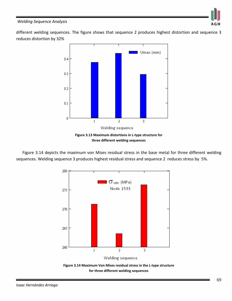
Welding Sequence Analysis
69 Isaac Hernández Arriaga
different welding sequences. The figure shows that sequence 2 produces highest distortion and sequence 3 reduces distortion by 32%
Figure 3.13 Maximum distortions in L-type structure for
three different welding sequences
Figure 3.14 depicts the maximum von Mises residual stress in the base metal for three different welding sequences. Welding sequence 3 produces highest residual stress and sequence 2 reduces stress by 5%.
Figure 3.14 Maximum Von Mises residual stress in the L-type structure
for three different welding sequences

Welding Sequence Analysis
70 Isaac Hernández Arriaga
3.18.1 Distortion profile in the L-type structure The maximum distortion occurs mainly in the Z-direction in the region near weld bead 2, and then decreases near weld beads 1 and 3 (Figure 3.15, welding sequence 3).
Figure 3.15 Distortion profile in the L-type structure corresponding to welding sequence 3
3.18.2 Residual stress distribution in the L-type structure The von Mises residual stress in the base metal is maximum at the boundary between the weld bead 2 and the vertical bar. High residual stresses also occur near the rigid base, close to weld beads 1 and 3. These residual stresses occur because weld beads 1 and 3 are highly constrained. In addition, these residual stresses change little with the welding sequence. Therefore, they are not considered for the welding sequence analysis. Figure 3.16 depicts the distribution of Von Mises residual stresses corresponding to welding sequence 2.
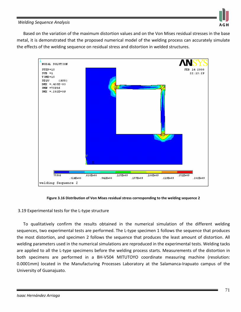
Welding Sequence Analysis
71 Isaac Hernández Arriaga
Based on the variation of the maximum distortion values and on the Von Mises residual stresses in the base metal, it is demonstrated that the proposed numerical model of the welding process can accurately simulate the effects of the welding sequence on residual stress and distortion in welded structures.
Figure 3.16 Distribution of Von Mises residual stress corresponding to the welding sequence 2
3.19 Experimental tests for the L-type structure To qualitatively confirm the results obtained in the numerical simulation of the different welding sequences, two experimental tests are performed. The L-type specimen 1 follows the sequence that produces the most distortion, and specimen 2 follows the sequence that produces the least amount of distortion. All welding parameters used in the numerical simulations are reproduced in the experimental tests. Welding tacks are applied to all the L-type specimens before the welding process starts. Measurements of the distortion in both specimens are performed in a BH-V504 MITUTOYO coordinate measuring machine (resolution: 0.0001mm) located in the Manufacturing Processes Laboratory at the Salamanca-Irapuato campus of the University of Guanajuato.
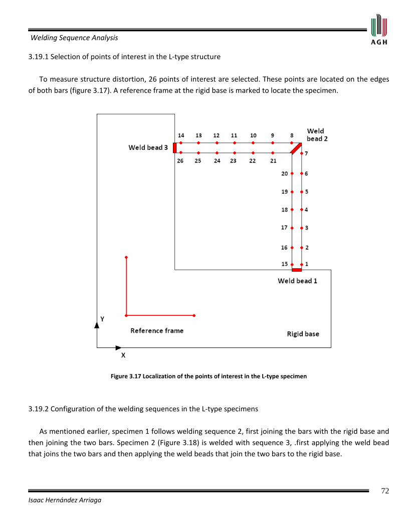
Welding Sequence Analysis
72 Isaac Hernández Arriaga
3.19.1 Selection of points of interest in the L-type structure To measure structure distortion, 26 points of interest are selected. These points are located on the edges of both bars (figure 3.17). A reference frame at the rigid base is marked to locate the specimen.
Figure 3.17 Localization of the points of interest in the L-type specimen
3.19.2 Configuration of the welding sequences in the L-type specimens As mentioned earlier, specimen 1 follows welding sequence 2, first joining the bars with the rigid base and then joining the two bars. Specimen 2 (Figure 3.18) is welded with sequence 3, .first applying the weld bead that joins the two bars and then applying the weld beads that join the two bars to the rigid base.
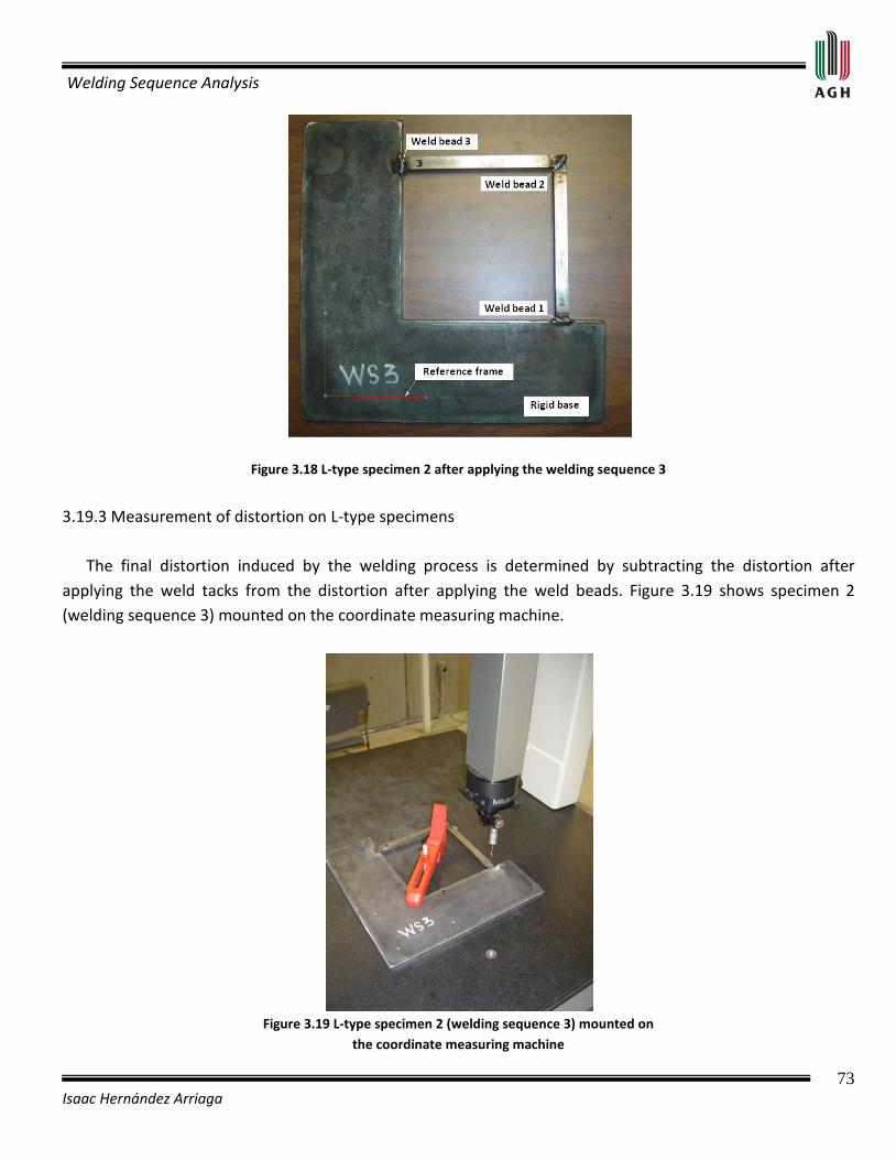
Welding Sequence Analysis
73 Isaac Hernández Arriaga
Figure 3.18 L-type specimen 2 after applying the welding sequence 3
3.19.3 Measurement of distortion on L-type specimens The final distortion induced by the welding process is determined by subtracting the distortion after applying the weld tacks from the distortion after applying the weld beads. Figure 3.19 shows specimen 2 (welding sequence 3) mounted on the coordinate measuring machine.
Figure 3.19 L-type specimen 2 (welding sequence 3) mounted on
the coordinate measuring machine
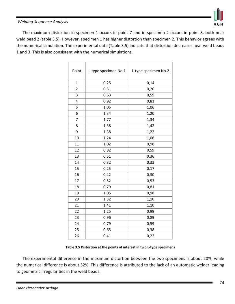
Welding Sequence Analysis
74 Isaac Hernández Arriaga
The maximum distortion in specimen 1 occurs in point 7 and in specimen 2 occurs in point 8, both near weld bead 2 (table 3.5). However, specimen 1 has higher distortion than specimen 2. This behavior agrees with the numerical simulation. The experimental data (Table 3.5) indicate that distortion decreases near weld beads 1 and 3. This is also consistent with the numerical simulations.
Point
L-type specimen No.1
L-type specimen No.2
1 0,25 0,14
2 0,51 0,26
3 0,63 0,59
4 0,92 0,81
5 1,05 1,06
6 1,34 1,20
7 1,77 1,34
8 1,58 1,42
9 1,38 1,22
10 1,24 1,06
11 1,02 0,98
12 0,82 0,59
13 0,51 0,36
14 0,32 0,33
15 0,25 0,17
16 0,42 0,30
17 0,52 0,53
18 0,79 0,81
19 1,05 0,98
20 1,32 1,10
21 1,41 1,10
22 1,25 0,99
23 0,96 0,89
24 0,79 0,59
25 0,65 0,38
26 0,41 0,22
Table 3.5 Distortion at the points of interest in two L-type specimens
The experimental difference in the maximum distortion between the two specimens is about 20%, while the numerical difference is about 32%. This difference is attributed to the lack of an automatic welder leading to geometric irregularities in the weld beads.
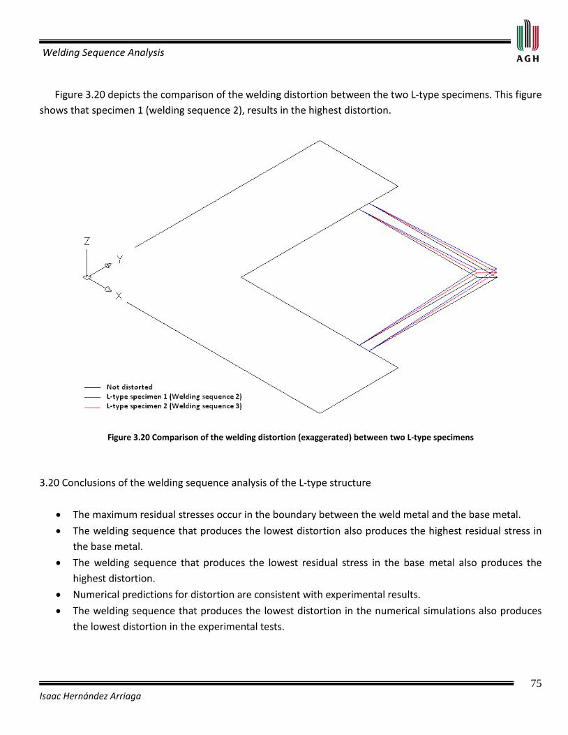
Welding Sequence Analysis
75 Isaac Hernández Arriaga
Figure 3.20 depicts the comparison of the welding distortion between the two L-type specimens. This figure shows that specimen 1 (welding sequence 2), results in the highest distortion.
Figure 3.20 Comparison of the welding distortion (exaggerated) between two L-type specimens
3.20 Conclusions of the welding sequence analysis of the L-type structure
• The maximum residual stresses occur in the boundary between the weld metal and the base metal.
• The welding sequence that produces the lowest distortion also produces the highest residual stress in the base metal.
• The welding sequence that produces the lowest residual stress in the base metal also produces the highest distortion.
• Numerical predictions for distortion are consistent with experimental results.
• The welding sequence that produces the lowest distortion in the numerical simulations also produces the lowest distortion in the experimental tests.
Welding Sequence Analysis
76 Isaac Hernández Arriaga
CHAPTER IV
WELDING SEQUENCE ANALYSIS IN A STIFFENED SYMMETRICAL
2-DIMENSIONAL FRAME 4.1 Introduction This chapter presents a study of the effects of the welding sequence on residual stresses and distortion in a stiffened symmetrical flat frame. The proper welding sequences obtained in this analysis are chosen to reduce residual stresses, distortion, or the relation between them. These proper welding sequences are obtained with the help of empirical welding rules: the axis of symmetry, center of gravity of the frame, and concentric circle. The origin of the circles coincides with the center of gravity of the flat frame, and the radius of the circles is formed by the center of gravity of the flat frame with the center of gravity of each of the weld beads. To carry out the different welding sequences, the numerical model developed in chapter 3 is used with the help of a commercial code. At the end of this chapter we propose and demonstrate a hypothesis to determine the proper welding sequences to reduce residual stress, distortion, or the relation between them for 2-dimensional symmetrical structures. 4.2 Geometric configuration of a stiffened symmetrical flat frame The proposed symmetrical flat structure has the shape of a stiffened frame consisting of four external bars and three internal bars joined by ten weld beads (Figure 4.1). This configuration is selected due to its multiple symmetries. The numbering of the weld beads is random.
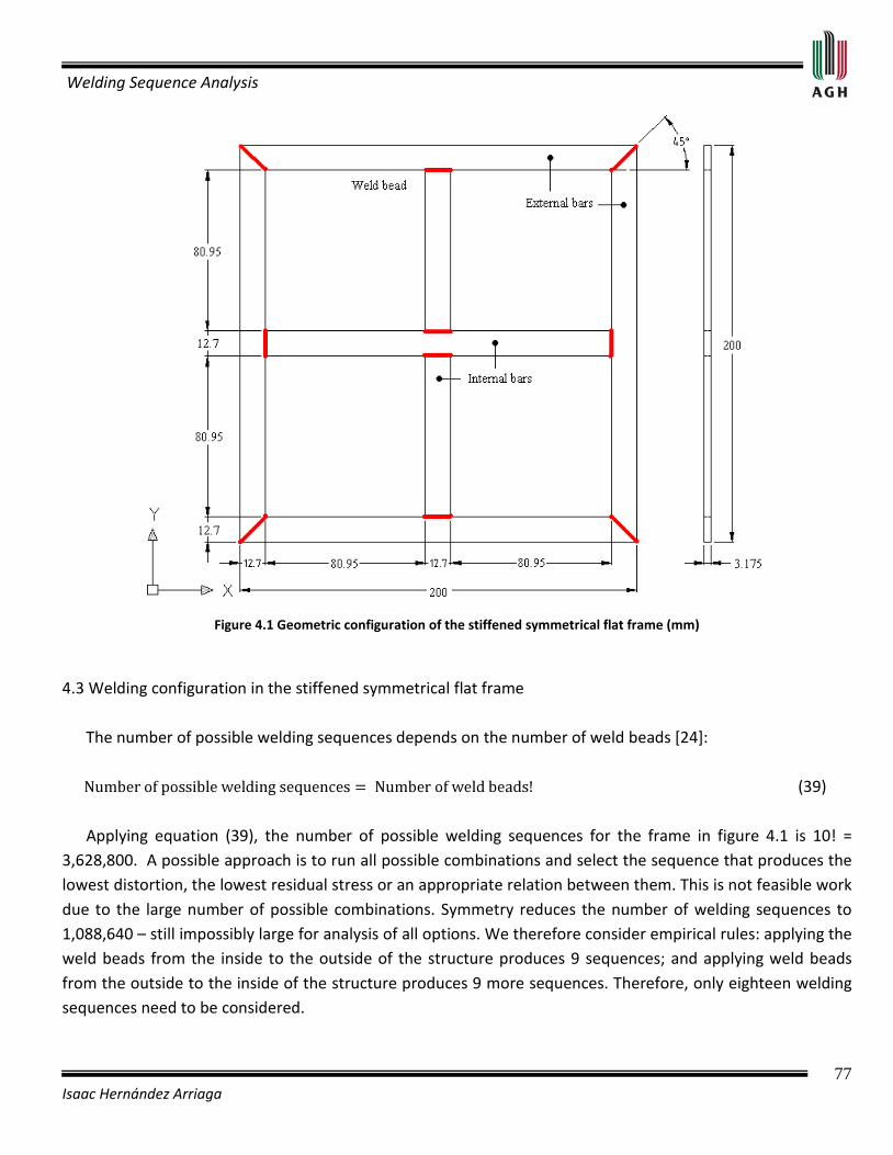
Welding Sequence Analysis
77 Isaac Hernández Arriaga
Figure 4.1 Geometric configuration of the stiffened symmetrical flat frame (mm)
4.3 Welding configuration in the stiffened symmetrical flat frame The number of possible welding sequences depends on the number of weld beads [24]: (39) Applying equation (39), the number of possible welding sequences for the frame in figure 4.1 is 10! = 3,628,800. A possible approach is to run all possible combinations and select the sequence that produces the lowest distortion, the lowest residual stress or an appropriate relation between them. This is not feasible work due to the large number of possible combinations. Symmetry reduces the number of welding sequences to 1,088,640 – still impossibly large for analysis of all options. We therefore consider empirical rules: applying the weld beads from the inside to the outside of the structure produces 9 sequences; and applying weld beads from the outside to the inside of the structure produces 9 more sequences. Therefore, only eighteen welding sequences need to be considered.
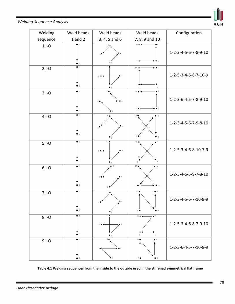
Welding Sequence Analysis
78 Isaac Hernández Arriaga
Welding sequence
Weld beads 1 and 2
Weld beads 3, 4, 5 and 6
Weld beads 7, 8, 9 and 10
Configuration
1 I-O
1-2-3-4-5-6-7-8-9-10
2 I-O
1-2-5-3-4-6-8-7-10-9
3 I-O
1-2-3-6-4-5-7-8-9-10
4 I-O
1-2-3-4-5-6-7-9-8-10
5 I-O
1-2-5-3-4-6-8-10-7-9
6 I-O
1-2-3-4-6-5-9-7-8-10
7 I-O
1-2-3-4-5-6-7-10-8-9
8 I-O
1-2-5-3-4-6-8-7-9-10
9 I-O
1-2-3-6-4-5-7-10-8-9
Table 4.1 Welding sequences from the inside to the outside used in the stiffened symmetrical flat frame

Welding Sequence Analysis
79 Isaac Hernández Arriaga
Welding sequence
Weld beads 7, 8, 9 Y 10
Weld beads 3, 4, 5 Y 6
Weld beads 1 Y 2
Configuration
1 O-I
10-9-8-7-6-5-4-3-2-1
2 O-I
9-10-7-8-6-4-3-5-2-1
3 O-I
10-9-8-7-5-4-6-3-2-1
4 O-I
10-8-9-7-6-5-4-3-2-1
5 O-I
9-7-10-8-6-4-3-5-2-1
6 O-I
10-8-7-9-5-6-4-3-2-1
7 O-I
9-8-10-7-6-5-4-3-2-1
8 O-I
10-9-7-8-6-4-3-5-2-1
9 O-I
9-8-10-7-5-4-6-3-2-1
Table 4.2 Welding sequences from the outside to the inside used in the stiffened symmetrical flat frame
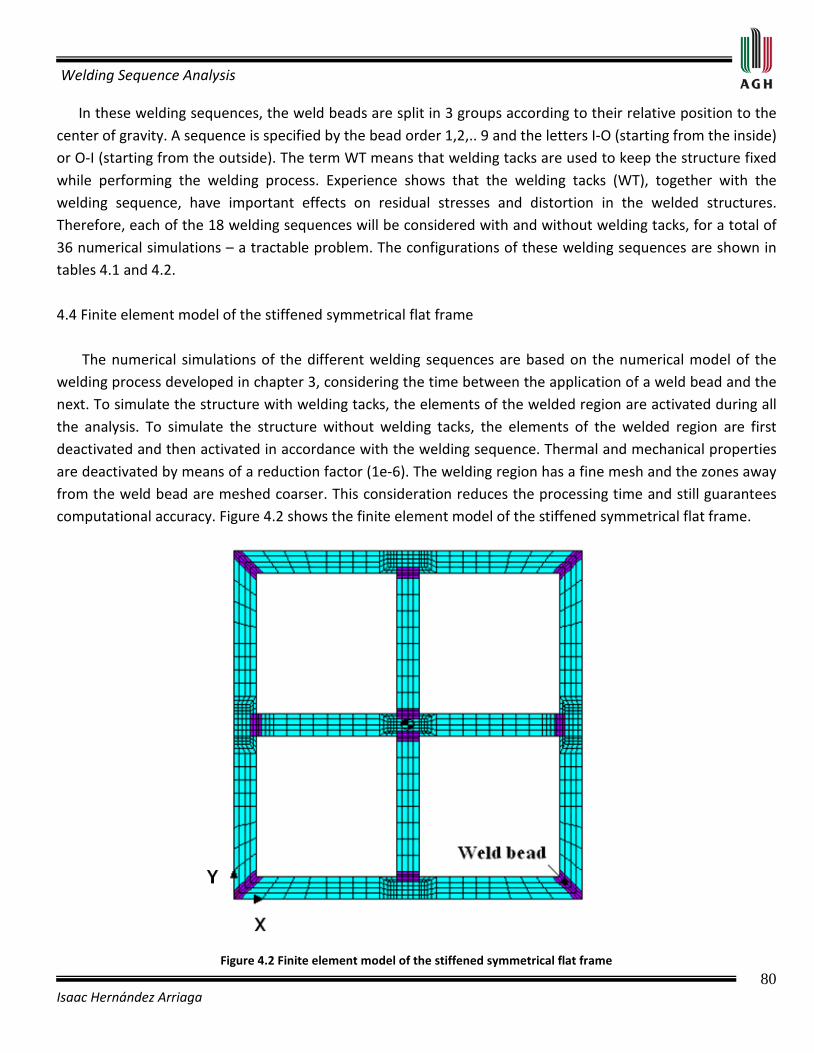
Welding Sequence Analysis
80 Isaac Hernández Arriaga
In these welding sequences, the weld beads are split in 3 groups according to their relative position to the center of gravity. A sequence is specified by the bead order 1,2,.. 9 and the letters I-O (starting from the inside) or O-I (starting from the outside). The term WT means that welding tacks are used to keep the structure fixed while performing the welding process. Experience shows that the welding tacks (WT), together with the welding sequence, have important effects on residual stresses and distortion in the welded structures. Therefore, each of the 18 welding sequences will be considered with and without welding tacks, for a total of 36 numerical simulations – a tractable problem. The configurations of these welding sequences are shown in tables 4.1 and 4.2. 4.4 Finite element model of the stiffened symmetrical flat frame The numerical simulations of the different welding sequences are based on the numerical model of the welding process developed in chapter 3, considering the time between the application of a weld bead and the next. To simulate the structure with welding tacks, the elements of the welded region are activated during all the analysis. To simulate the structure without welding tacks, the elements of the welded region are first deactivated and then activated in accordance with the welding sequence. Thermal and mechanical properties are deactivated by means of a reduction factor (1e-6). The welding region has a fine mesh and the zones away from the weld bead are meshed coarser. This consideration reduces the processing time and still guarantees computational accuracy. Figure 4.2 shows the finite element model of the stiffened symmetrical flat frame.
Figure 4.2 Finite element model of the stiffened symmetrical flat frame

Welding Sequence Analysis
81 Isaac Hernández Arriaga
4.4.1 Thermal initial and boundary conditions a) Initial condition: Because the thermal model consists of a transient heat transfer analysis, it is required an initial condition of the base metal, which is considered as the surrounding temperature ( =20°C). b) Boundary conditions (see figure 4.2, page 80): Surfaces in contact with the surrounding except surfaces belonging to the weld beads (Plane x-y in z=0):
Nodes belonging to weld beads (according to the welding sequence): Prescribed heat input: heat loading is simulated via weld thermal cycle curves (figure 3.6, page 60). Heat is applied on all surfaces between the weld metal and the base metal according to welding sequence. 4.4.2 Mechanical boundary conditions Three boundary conditions are applied to structural model: a) those just sufficient to prevent rigid body motion and rotations of the model and b) stress-free on Z-direction (plane-stress problem), which imply that all out-of-plane stresses vanish, and c) the normal stresses to the surfaces in contact with the surrounding and the shear stresses are zero. a) The nodes belonging to the element attached to its center of gravity of the structure are selected to prevent rigid body motion and rigid body rotations (see figure 4.2, page 80):
; ; ; and
b) In the plane-stress problem, the normal stresses to the plane X-Y ( ) and shearing stress acting in this plane ( and ) are zero on face of the structure (see figure 4.2, page 80). Therefore, . c) Surfaces in contact with the surrounding (see figure 4.2, page 80): The normal stresses to the surfaces in contact with the surrounding and the shear stresses are zero (i.e., in x=0, ).
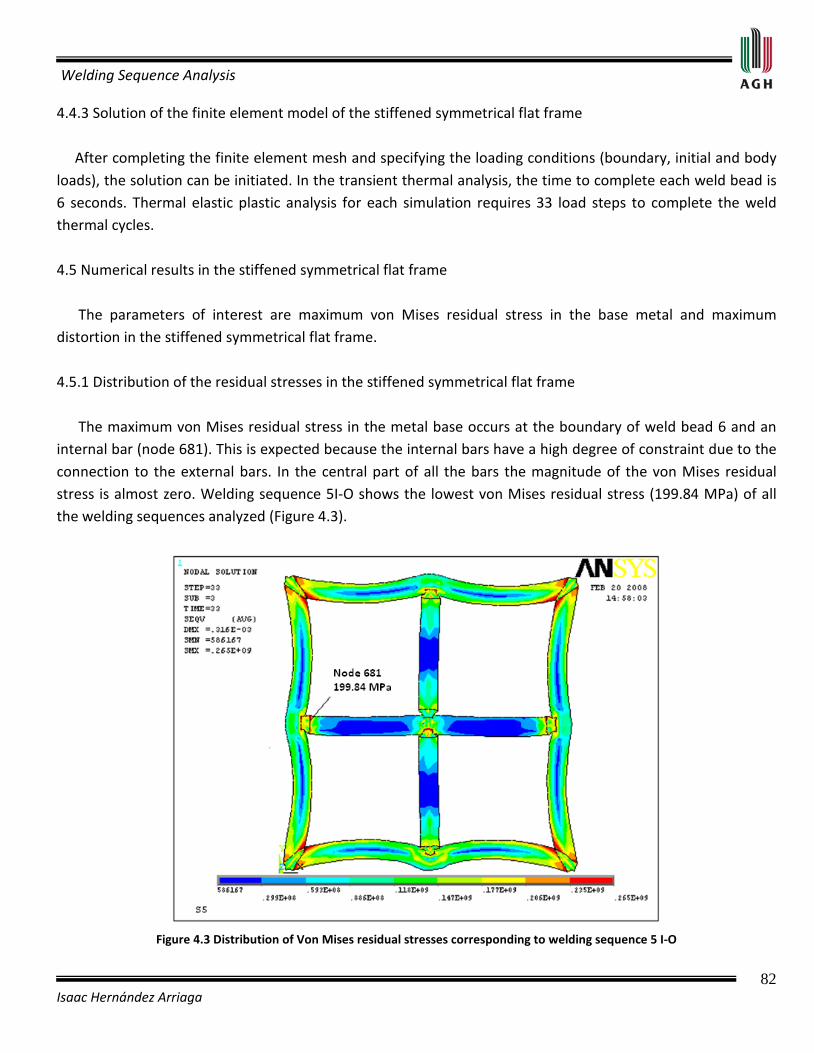
Welding Sequence Analysis
82 Isaac Hernández Arriaga
4.4.3 Solution of the finite element model of the stiffened symmetrical flat frame After completing the finite element mesh and specifying the loading conditions (boundary, initial and body loads), the solution can be initiated. In the transient thermal analysis, the time to complete each weld bead is 6 seconds. Thermal elastic plastic analysis for each simulation requires 33 load steps to complete the weld thermal cycles. 4.5 Numerical results in the stiffened symmetrical flat frame The parameters of interest are maximum von Mises residual stress in the base metal and maximum distortion in the stiffened symmetrical flat frame. 4.5.1 Distribution of the residual stresses in the stiffened symmetrical flat frame The maximum von Mises residual stress in the metal base occurs at the boundary of weld bead 6 and an internal bar (node 681). This is expected because the internal bars have a high degree of constraint due to the connection to the external bars. In the central part of all the bars the magnitude of the von Mises residual stress is almost zero. Welding sequence 5I-O shows the lowest von Mises residual stress (199.84 MPa) of all the welding sequences analyzed (Figure 4.3).
Figure 4.3 Distribution of Von Mises residual stresses corresponding to welding sequence 5 I-O
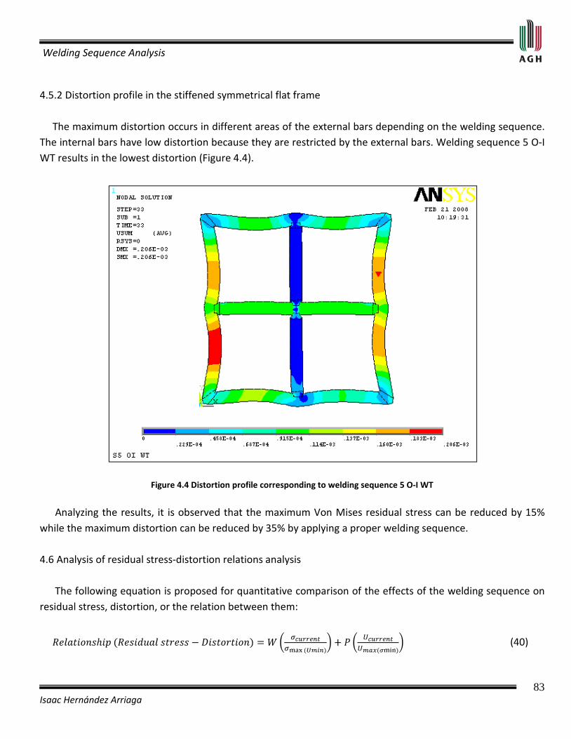
Welding Sequence Analysis
83 Isaac Hernández Arriaga
4.5.2 Distortion profile in the stiffened symmetrical flat frame The maximum distortion occurs in different areas of the external bars depending on the welding sequence. The internal bars have low distortion because they are restricted by the external bars. Welding sequence 5 O-I WT results in the lowest distortion (Figure 4.4).
Figure 4.4 Distortion profile corresponding to welding sequence 5 O-I WT
Analyzing the results, it is observed that the maximum Von Mises residual stress can be reduced by 15% while the maximum distortion can be reduced by 35% by applying a proper welding sequence. 4.6 Analysis of residual stress-distortion relations analysis The following equation is proposed for quantitative comparison of the effects of the welding sequence on residual stress, distortion, or the relation between them:
(40)
Welding Sequence Analysis
84 Isaac Hernández Arriaga
Where: and are the residual stress and distortion for each welding sequence. The residual stress corresponds to one selected point on the structure and the distortion corresponds to the maximum distortion that occurs in each welding sequence. The highest residual stress that occurs in all welding sequences is accompanied by lowest distortion. The highest distortion that occurs in all welding
sequences , is accompanied by lowest residual stress. Weight factors W and P can be assigned to
residual stress and distortion, respectively. For the case when the welding sequence only reduces the residual stress, and . When the welding sequence only reduces distortion, and . When the welding sequence reduces the relation between both parameters, . 4.7 Order of importance of the welding sequences to reduce residual stress, distortion, or the relation between them in the stiffened symmetrical flat frame Applying equation (40) [page 83] to the results of the residual stress and distortion obtained in the 36 numerical simulations, the order of importance of the different welding sequences to reduce residual stress, distortion, or a relation between them is obtained (table 4.3). Analyzing these results, the proper welding sequence to reduce residual stress is 5 I-O (from the inside to the outside of the structure), and the proper welding sequence to reduce the distortion is 5 O-I WT (from the outside to the inside using welding tacks). This implies that the proper welding sequence to reduce the residual stresses is inappropriate to reduce the distortion and vice versa. Finally, welding sequence 1 I-O (welding sequence in growing spiral) shows the best overall performance: it is ranked number 4 in reducing stress and 19 in reducing distortion. Therefore, welding sequence 1 I-O is the proper welding sequence to improve the relation between the selected critical parameters. 4.8 Proper welding sequences to reduce the residual stress, distortion, or a relation between them in the stiffened symmetrical flat frame To formulate the proper welding sequences obtained in table 4.3, the axis of symmetry and the center of gravity of the flat frame are used. We draw concentric circles centered on the center of gravity of the frame and extending to the center of gravity of the weld beads. The weld beads located at the same distance from the center of gravity of the frame fall on the same circle. The circles are numbered from the smallest to the largest. Weld beads 1 and 2 belong to circle 1, weld beads 3, 4, 5, and 6 belong to circle 2, and weld beads 7, 8, 9, and 10 belong to circle 3 (Figure 4.5).
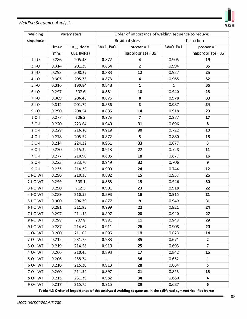
Welding Sequence Analysis
85 Isaac Hernández Arriaga
Welding sequence
Parameters Order of importance of welding sequence to reduce:
Residual stress Distortion
Umax (mm)
σvm W=1, P=0 Node 681 (MPa)
proper = 1 inappropriate= 36
W=0, P=1 proper = 1 inappropriate= 36
1 I-O 0.286 205.48 0.872 4 0.905 19
2 I-O 0.314 201.29 0.854 2 0.994 35
3 I-O 0.293 208.27 0.883 12 0.927 25
4 I-O 0.305 205.73 0.873 6 0.965 32
5 I-O 0.316 199.84 0.848 1 1 36
6 I-O 0.297 207.6 0.881 10 0.940 28
7 I-O 0.309 206.46 0.876 8 0.978 33
8 I-O 0.312 201.72 0.856 3 0.987 34
9 I-O 0.290 208.54 0.885 14 0.918 23
1 O-I 0.277 206.3 0.875 7 0.877 17
2 O-I 0.220 223.64 0.949 31 0.696 8
3 O-I 0.228 216.30 0.918 30 0.722 10
4 O-I 0.278 205.52 0.872 5 0.880 18
5 O-I 0.214 224.22 0.951 33 0.677 3
6 O-I 0.230 215.32 0.913 27 0.728 11
7 O-I 0.277 210.90 0.895 18 0.877 16
8 O-I 0.223 223.70 0.949 32 0.706 9
9 O-I 0.235 214.29 0.909 24 0.744 12
1 I-O WT 0.296 210.33 0.892 15 0.937 26
2 I-O WT 0.299 208.1 0.883 13 0.946 30
3 I-O WT 0.290 212.3 0.901 23 0.918 22
4 I-O WT 0.289 210.53 0.893 16 0.915 21
5 I-O WT 0.300 206.79 0.877 9 0.949 31
6 I-O WT 0.291 211.95 0.899 22 0.921 24
7 I-O WT 0.297 211.43 0.897 20 0.940 27
8 I-O WT 0.298 207.8 0.881 11 0.943 29
9 I-O WT 0.287 214.67 0.911 26 0.908 20
1 O-I WT 0.260 211.05 0.895 19 0.823 14
2 O-I WT 0.212 231.75 0.983 35 0.671 2
3 O-I WT 0.219 214.58 0.910 25 0.693 7
4 O-I WT 0.266 210.45 0.893 17 0.842 15
5 O-I WT 0.206 235.74 1 36 0.652 1
6 O-I WT 0.216 215.20 0.913 28 0.684 5
7 O-I WT 0.260 211.52 0.897 21 0.823 13
8 O-I WT 0.215 231.39 0.982 34 0.680 4
9 O-I WT 0.217 215.75 0.915 29 0.687 6 Table 4.3 Order of importance of the analyzed welding sequences in the stiffened symmetrical flat frame
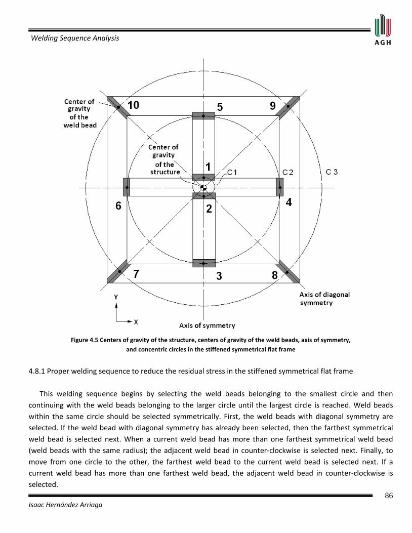
Welding Sequence Analysis
86 Isaac Hernández Arriaga
Figure 4.5 Centers of gravity of the structure, centers of gravity of the weld beads, axis of symmetry,
and concentric circles in the stiffened symmetrical flat frame
4.8.1 Proper welding sequence to reduce the residual stress in the stiffened symmetrical flat frame This welding sequence begins by selecting the weld beads belonging to the smallest circle and then continuing with the weld beads belonging to the larger circle until the largest circle is reached. Weld beads within the same circle should be selected symmetrically. First, the weld beads with diagonal symmetry are selected. If the weld bead with diagonal symmetry has already been selected, then the farthest symmetrical weld bead is selected next. When a current weld bead has more than one farthest symmetrical weld bead (weld beads with the same radius); the adjacent weld bead in counter-clockwise is selected next. Finally, to move from one circle to the other, the farthest weld bead to the current weld bead is selected next. If a current weld bead has more than one farthest weld bead, the adjacent weld bead in counter-clockwise is selected.
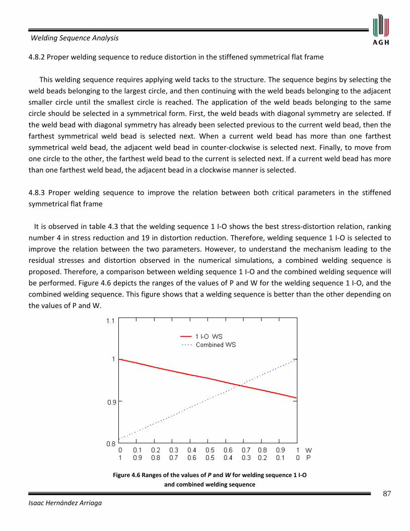
Welding Sequence Analysis
87 Isaac Hernández Arriaga
4.8.2 Proper welding sequence to reduce distortion in the stiffened symmetrical flat frame This welding sequence requires applying weld tacks to the structure. The sequence begins by selecting the weld beads belonging to the largest circle, and then continuing with the weld beads belonging to the adjacent smaller circle until the smallest circle is reached. The application of the weld beads belonging to the same circle should be selected in a symmetrical form. First, the weld beads with diagonal symmetry are selected. If the weld bead with diagonal symmetry has already been selected previous to the current weld bead, then the farthest symmetrical weld bead is selected next. When a current weld bead has more than one farthest symmetrical weld bead, the adjacent weld bead in counter-clockwise is selected next. Finally, to move from one circle to the other, the farthest weld bead to the current is selected next. If a current weld bead has more than one farthest weld bead, the adjacent bead in a clockwise manner is selected. 4.8.3 Proper welding sequence to improve the relation between both critical parameters in the stiffened symmetrical flat frame It is observed in table 4.3 that the welding sequence 1 I-O shows the best stress-distortion relation, ranking number 4 in stress reduction and 19 in distortion reduction. Therefore, welding sequence 1 I-O is selected to improve the relation between the two parameters. However, to understand the mechanism leading to the residual stresses and distortion observed in the numerical simulations, a combined welding sequence is proposed. Therefore, a comparison between welding sequence 1 I-O and the combined welding sequence will be performed. Figure 4.6 depicts the ranges of the values of P and W for the welding sequence 1 I-O, and the combined welding sequence. This figure shows that a welding sequence is better than the other depending on the values of P and W.
Figure 4.6 Ranges of the values of P and W for welding sequence 1 I-O
and combined welding sequence
Welding Sequence Analysis
88 Isaac Hernández Arriaga
For: and This welding sequence starts with the beads in the smallest circle and then continuing with the beads in the larger adjacent circle until the largest circle is reached. Weld beads within the same circle should be applied in counter-clockwise direction. To move from one circle to the next, the closest weld bead is selected. For: and In this welding sequence, welding tacks are required only on the circle next to the larger adjacent circle. The sequence begins by selecting the weld beads on the smallest circle, and then continuing with the weld beads on the circle next to the larger adjacent circle and continuing with the beads on the smaller adjacent circle. The application of the beads on the same circle should be symmetrical. First, the weld beads with diagonal symmetry are applied. If the weld bead with diagonal symmetry has already been applied, then the farthest symmetrical weld bead is selected next. When a current weld bead has more than one farthest symmetrical bead, the adjacent bead in counter-clockwise direction is selected next. Finally, to move from one circle to the other, the farthest weld bead to the current bead is selected next. If a current weld bead has more than one farthest bead, the adjacent bead in counter-clockwise direction is selected. 4.9 Hypothesis to determine the proper welding sequence to reduce the residual stress, distortion, or a relation between them in symmetrical flat structures To determine the proper welding sequences to reduce the residual stress, distortion, or a relation between them in flat symmetrical structures, it is necessary to determine the axis of symmetry and the center of gravity of the structure. We next draw concentric circles centered on the center of gravity of the structure and extending to the center of gravity of the weld beads. Weld beads that are located at the same distance from the center of gravity of the structure fall on the same circle. Circles are numbered from the smallest to the largest diameter. a) To reduce residual stress: Start with the weld beads on the smallest circle and then continue with the beads on the larger adjacent circle until the largest circle is reached. The weld beads on the same circle should be selected in a symmetrical form. First, the weld beads with diagonal symmetry are selected. If the bead with diagonal symmetry has already been selected, then the farthest symmetrical bead is selected. When a weld bead has more than one farthest symmetrical weld bead, the adjacent weld bead in counter-clockwise direction is selected. Finally, to move from one circle to the other, the farthest weld bead to the current weld bead is selected. If a current weld bead has more than one farthest weld bead, the adjacent weld bead in counter-clockwise direction is selected.

Welding Sequence Analysis
89 Isaac Hernández Arriaga
b) To reduce distortion: Apply welding tacks to the structure before welding. First, the weld beads in the largest circle are selected and then the beads on the adjacent smaller circle are selected until the smallest circle is reached. Beads on the same circle should be applied symmetrically. Beads with diagonal symmetry are selected first. If the weld bead with diagonal symmetry has already been previously selected, then the farthest symmetrical bead is selected next. When a current weld bead has more than one farthest symmetrical weld bead, the adjacent weld bead in counter-clockwise direction is selected next. Finally, to move from one circle to the other, the farthest weld bead is selected. If a current bead has more than one farthest bead, the adjacent bead in a clockwise manner is selected. c) To improve the relation between residual stress and distortion: i) Favoring the residual stress: Start with the weld beads belonging to the smallest circle and then continuing with the beads on the larger adjacent circle until the largest circle is reached. The application of weld beads belonging to the same circle should counterclockwise into adjacent beads. To move from one circle to the other, the closest weld bead to the current weld bead is selected. ii) Favoring the distortion: This welding sequence requires application of welding tacks only on the circle next to the larger adjacent circle. The welding sequence starts by selecting the beads on the smallest circle, and then continuing with the beads on the circle next to the larger adjacent circle, and later going back to the beads on the smaller adjacent circle. The application of the weld beads on the same circle should be in a symmetrical form. First, the beads with diagonal symmetry are applied. If the weld bead with diagonal symmetry has already been applied, then the farthest symmetrical bead is selected next. When a current bead has more than one farthest symmetrical bead, the adjacent bead in counter-clockwise direction is selected next. Finally, to move from one circle to the other, the farthest bead to the current is selected next. If a current weld bead has more than one farthest bead, the adjacent bead in counter-clockwise direction is selected. For the stiffened symmetrical flat frame, the hypothesis to determine the proper welding sequence to reduce residual stress, distortion, or the relation between them in symmetrical structures in the plane is verified. 4.10 Experimental tests in a stiffened symmetrical flat frame specimen We conducted an experiment to validate the numerical results. All welding parameters used in the numerical simulations are reproduced in the experiment. Welding tacks are applied to a stiffened symmetrical flat specimen before the welding process starts. Measurement of the distortion in the stiffened symmetrical plane specimen is performed in a BH-V504 MITUTOYO coordinate measuring machine (resolution: 0.0001 mm). This machine is located in the manufacture laboratory at the University of Guanajuato campus Salamanca-Irapuato.

Welding Sequence Analysis
90 Isaac Hernández Arriaga
4.10.1 Selection of points of interest in the stiffened symmetrical flat specimen To measure distortion, 88 points of interest are selected (Figure 4.7). These points are located on the edges of all bars. A reference frame at the internal horizontal bar is marked to position the stiffened symmetrical flat specimen.
Figure 4.7 Localization of the point of interest in the stiffened symmetrical flat specimen
4.10.2 Configuration of the welding sequence in the stiffened symmetrical flat specimen As previously mentioned, the stiffened symmetrical flat specimen follows the welding sequence that minimizes distortion (5 O-I WT, Table 4.4 and figure 4.8). This sequence first applies beads at locations farthest from the center and then moves progressively inward. Weld beads at equal distance from the center of the specimen are selected symmetrically.
Welding sequence Configuration
5 O-I WT 9-7-10-8-6-4-3-5-2-1 Table 4.4 Configuration of welding sequence 5 O-I WT
used in the stiffened symmetrical flat specimen
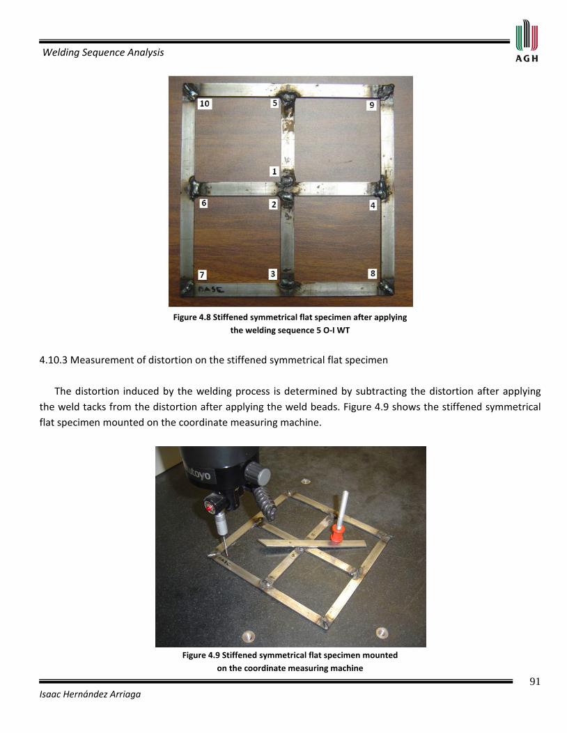
Welding Sequence Analysis
91 Isaac Hernández Arriaga
Figure 4.8 Stiffened symmetrical flat specimen after applying
the welding sequence 5 O-I WT
4.10.3 Measurement of distortion on the stiffened symmetrical flat specimen The distortion induced by the welding process is determined by subtracting the distortion after applying the weld tacks from the distortion after applying the weld beads. Figure 4.9 shows the stiffened symmetrical flat specimen mounted on the coordinate measuring machine.
Figure 4.9 Stiffened symmetrical flat specimen mounted
on the coordinate measuring machine
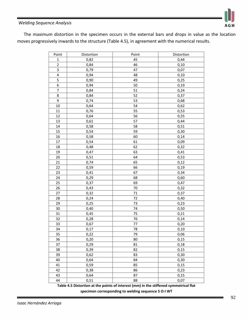
Welding Sequence Analysis
92 Isaac Hernández Arriaga
The maximum distortion in the specimen occurs in the external bars and drops in value as the location moves progressively inwards to the structure (Table 4.5), in agreement with the numerical results.
Point Distortion Point Distortion 1 0,82 45 0,44 2 0,84 46 0,10 3 0,79 47 0,07 4 0,94 48 0,10 5 0,90 49 0,25 6 0,94 50 0,19 7 0,84 51 0,24 8 0,84 52 0,37 9 0,74 53 0,68
10 0,64 54 0,62 11 0,76 55 0,53 12 0,64 56 0,55 13 0,61 57 0,44 14 0,58 58 0,51 15 0,54 59 0,30 16 0,58 60 0,14 17 0,54 61 0,09 18 0,48 62 0,32 19 0,47 63 0,41 20 0,51 64 0,53 21 0,74 65 0,12 22 0,59 66 0,19 23 0,41 67 0,34 24 0,29 68 0,60 25 0,37 69 0,47 26 0,43 70 0,32 27 0,32 71 0,37 28 0,24 72 0,40 29 0,25 73 0,23 30 0,40 74 0,50 31 0,45 75 0,21 32 0,28 76 0,14 33 0,67 77 0,20 34 0,17 78 0,10 35 0,22 79 0,06 36 0,20 80 0,15 37 0,29 81 0,18 38 0,39 82 0,15 39 0,62 83 0,30 40 0,64 84 0,30 41 0,59 85 0,15 42 0,38 86 0,23 43 0,64 87 0,15 44 0,51 88 0,07 Table 4.5 Distortion at the points of interest (mm) in the stiffened symmetrical flat
specimen corresponding to welding sequence 5 O-I WT

Welding Sequence Analysis
93 Isaac Hernández Arriaga
The maximum measured distortion is four times higher in the Z-direction. This is probably because the welding process was not automated, producing geometric irregularities in the weld bead. Figure 4.10 depicts the measured distortion profile, indicating that the maximum distortion occurs on the external bars and progressively decreases as it approaches to center of the specimen.
Figure 4.10 Distortion profile in the stiffened symmetrical flat specimen corresponding to welding sequence 5 O-I WT (exaggerated)
4.11 Conclusions of the welding sequence analysis of stiffened symmetrical flat frame
• The maximum residual stress in the metal base occurs in the boundary with the welded metal in the internal bars.
• For the stiffened symmetrical flat frame, the distortion is reduced by 35 %, while the maximum von Mises residual stress is reduced by 15% when applying the proper welding sequence to respectively reduce distortion or residual stress. The welding sequence is twice as effective for reducing distortion than for reducing residual stresses.
• Welding tacks are not recommended when trying to reduce residual stress.
• Welding tacks are necessary to reduce distortion.

Welding Sequence Analysis
94 Isaac Hernández Arriaga
• Welding tacks followed by weld bead application from the outside to the inside of the structure reduces distortion but increases residual stresses.
• Applying the weld beads from the inside to the outside of the structure without welding tacks reduces the residual stress but increases the distortion.
• The welding sequence that produces the lowest distortion also produces the highest residual stress.
• The welding sequence that produces the lowest residual stress also produces the highest distortion.
• The relation between P=0,5 and W=0,5 does not mean that both parameters are reduced by the same percentage, because the proper welding sequence reduces the distortion twice as much as residual stresses.
• There is good qualitative agreement between the measured and numerical results. Quantitatively, however, the numerical results show lower maximum peak values. The difference is probably due to the lack of an automated welder.
Welding Sequence Analysis
95 Isaac Hernández Arriaga
CHAPTER V
WELDING SEQUENCE ANALYSIS IN A 3-DIMENSIONAL UNITARY CELL-TYPE
SYMMETRICAL STRUCTURE 5.1 Introduction This chapter describes a study of the effects of the welding sequence on the residual stresses and distortion in a 3-dimensional unitary cell, with the purpose of demonstrating that the methodology for determining the proper welding sequences to reduce residual stress, distortion, or the relation between them in 2-dimensional symmetrical structures can be applied to 3-dimensional symmetrical structures, where weld bead circles become spheres. The methodology is demonstrated by conducting four numerical simulations in the proposed symmetrical structure. Two of the numerical simulations deal with the proper welding sequence to reduce residual stress and the other two deals with the proper welding sequence to reduce distortion. A special welding sequence is also analyzed for comparison with the proper sequence to reduce distortion. This special welding sequence applies the external beads first and the internal beads later. All the numerical simulations are based on the proposed numerical model of the welding process developed in Chapter 3 with a commercial software code.
Welding Sequence Analysis
96 Isaac Hernández Arriaga
5.2 Hypothesis to determine the proper welding sequence to reduce the residual stress, distortion, or a relation between them in 3-dimensional symmetrical structures To determine the proper welding sequences to reduce the residual stress, distortion, or a relation between them in 3-dimensional symmetrical structures, we start by identifying the axis of symmetry and the center of gravity of the structure. Next, we draw concentric spheres centered on the center of gravity of the structure, and extending to the center of gravity of each of the weld beads. Weld beads located at the same distance from the center of gravity of the structure will fall on the same sphere. The spheres are numbered from the smallest to the largest. a) To reduce residual stress: Start with the weld beads belonging to the smallest sphere and then continue with the weld beads belonging to the larger adjacent sphere until the largest sphere is reached. The weld beads belonging to the same sphere should be symmetrical. First, the beads with diagonal symmetry are selected. If the weld bead with diagonal symmetry has already been selected, then the farthest symmetrical weld bead is selected next. When a current weld bead has more than one farthest symmetrical bead, the adjacent weld bead in counter-clockwise is selected. Finally, to move from one sphere to the other, the farthest weld bead to the current bead is selected. If a current bead has more than one farthest weld bead, the adjacent bead in counter-clockwise is selected. The converse welding method between weld beads is adopted. b) To reduce distortion: Apply welding tacks to the structure before welding. First, the weld beads in the largest sphere are selected and then the weld beads belonging to the adjacent smaller sphere are selected until the smallest sphere is reached. The application of the weld beads on the same sphere should be in symmetrical form. The weld beads with diagonal symmetry are selected first. If the weld bead with diagonal symmetry has already been selected, then the farthest symmetrical bead is selected next. When a weld bead has more than one farthest symmetrical bead, the adjacent weld bead in counter-clockwise direction is selected next. Finally, to move from one sphere to the other, the farthest weld bead to the current is selected. If a weld bead has more than one farthest bead, the adjacent bead in a clockwise direction is selected. The converse welding method between beads is adopted. c) To improve the relation between residual stress and distortion: i) Favoring residual stress: Start with the weld beads on the smallest sphere and then continue with the weld beads on the larger adjacent sphere until the largest sphere is reached. The application of weld beads on the same sphere should be in an adjacent form in counter-clockwise direction. To move from one sphere to the other, the closest weld bead to the current bead is selected. The converse welding method between weld beads is adopted.

Welding Sequence Analysis
97 Isaac Hernández Arriaga
ii) Favoring distortion: In this welding sequence, the application of welding tacks is required only on the sphere next to the larger adjacent sphere. The welding sequence begins by selecting the weld beads on the smallest sphere, and then continuing with the weld beads on the sphere next to the larger adjacent sphere. Then, going back to the weld beads on the smaller adjacent sphere. The application of the weld beads on the same sphere should be symmetrical. First, the weld beads with diagonal symmetry are applied. If the weld bead with diagonal symmetrical has already been applied, then the farthest symmetrical weld bead is selected next. When a current weld bead has more than one farthest symmetrical bead, the adjacent bead in counter-clockwise direction is selected next. Finally, to move from one sphere to the other, the farthest weld bead to the current weld bead is selected next. If a current weld bead has more than one farthest weld bead, the adjacent weld bead in counter-clockwise direction is selected. The converse welding method between weld beads is adopted. 5.3 Geometric configuration of the 3-dimensional unitary cell A 3-dimensional unitary cell configuration is selected because it is a common structural arrangement in industry, used in the construction of panels, ships, bridges, etc. This configuration keeps the requirement of symmetry in the space. Figure 5.1 depicts a structural panel used in the welding industry, where a segment takes the form of a 3-dimensional unitary cell.
Figure 5.1 Panel used in the welding industry
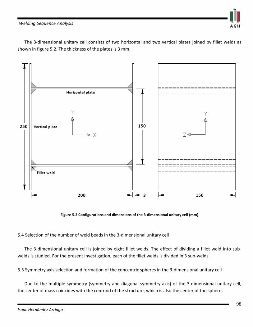
Welding Sequence Analysis
98 Isaac Hernández Arriaga
The 3-dimensional unitary cell consists of two horizontal and two vertical plates joined by fillet welds as shown in figure 5.2. The thickness of the plates is 3 mm.
Figure 5.2 Configurations and dimensions of the 3-dimensional unitary cell (mm)
5.4 Selection of the number of weld beads in the 3-dimensional unitary cell The 3-dimensional unitary cell is joined by eight fillet welds. The effect of dividing a fillet weld into sub-welds is studied. For the present investigation, each of the fillet welds is divided in 3 sub-welds. 5.5 Symmetry axis selection and formation of the concentric spheres in the 3-dimensional unitary cell Due to the multiple symmetry (symmetry and diagonal symmetry axis) of the 3-dimensional unitary cell, the center of mass coincides with the centroid of the structure, which is also the center of the spheres.
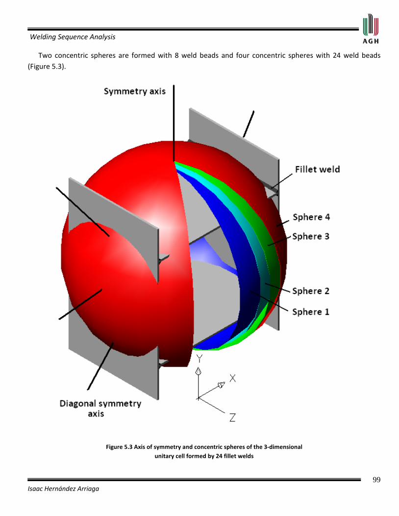
Welding Sequence Analysis
99 Isaac Hernández Arriaga
Two concentric spheres are formed with 8 weld beads and four concentric spheres with 24 weld beads (Figure 5.3).
Figure 5.3 Axis of symmetry and concentric spheres of the 3-dimensional unitary cell formed by 24 fillet welds
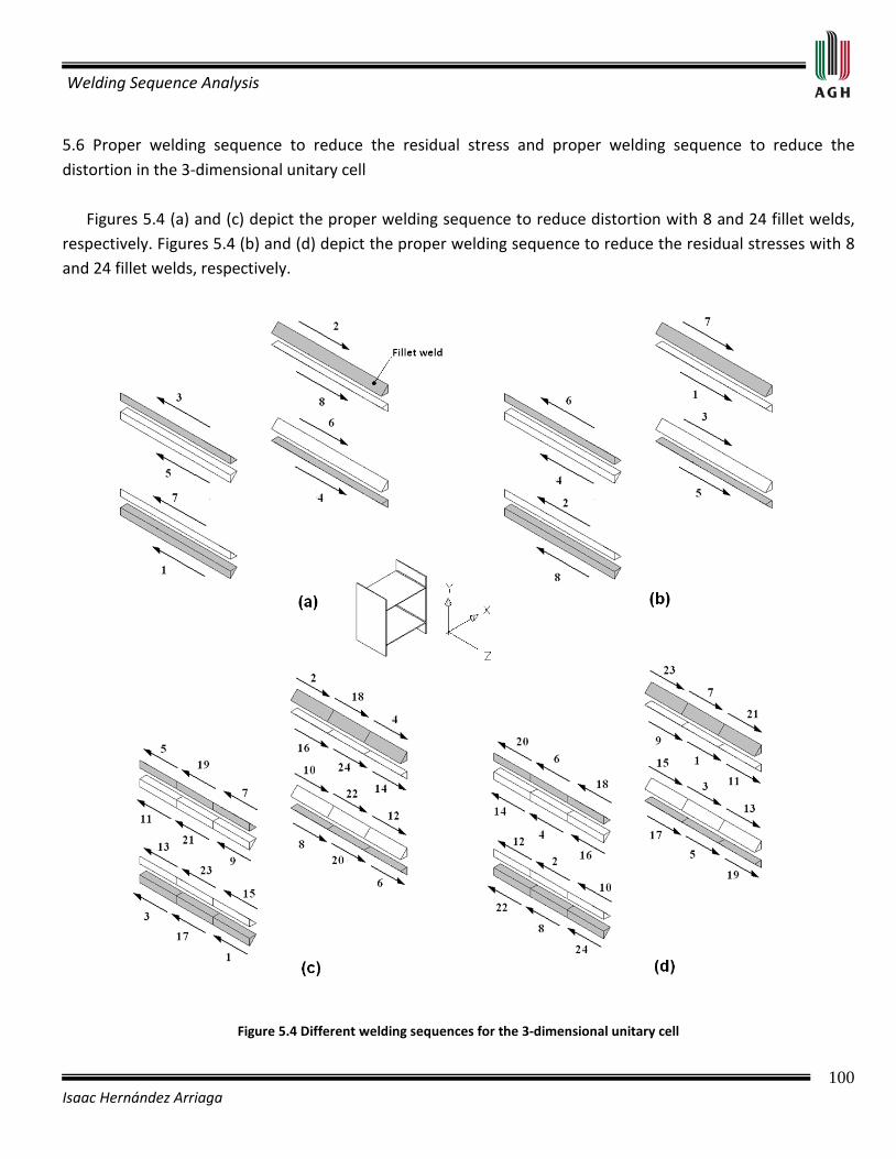
Welding Sequence Analysis
100 Isaac Hernández Arriaga
5.6 Proper welding sequence to reduce the residual stress and proper welding sequence to reduce the distortion in the 3-dimensional unitary cell Figures 5.4 (a) and (c) depict the proper welding sequence to reduce distortion with 8 and 24 fillet welds, respectively. Figures 5.4 (b) and (d) depict the proper welding sequence to reduce the residual stresses with 8 and 24 fillet welds, respectively.
Figure 5.4 Different welding sequences for the 3-dimensional unitary cell
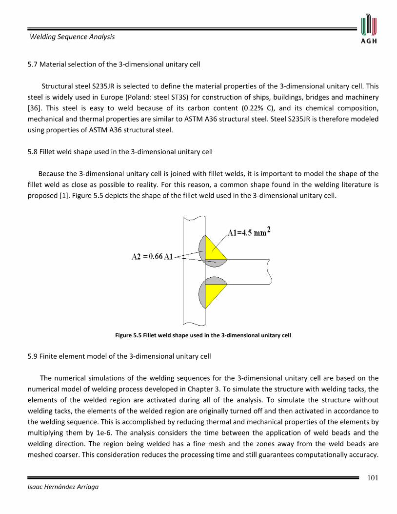
Welding Sequence Analysis
101 Isaac Hernández Arriaga
5.7 Material selection of the 3-dimensional unitary cell Structural steel S235JR is selected to define the material properties of the 3-dimensional unitary cell. This steel is widely used in Europe (Poland: steel ST3S) for construction of ships, buildings, bridges and machinery [36]. This steel is easy to weld because of its carbon content (0.22% C), and its chemical composition, mechanical and thermal properties are similar to ASTM A36 structural steel. Steel S235JR is therefore modeled using properties of ASTM A36 structural steel. 5.8 Fillet weld shape used in the 3-dimensional unitary cell Because the 3-dimensional unitary cell is joined with fillet welds, it is important to model the shape of the fillet weld as close as possible to reality. For this reason, a common shape found in the welding literature is proposed [1]. Figure 5.5 depicts the shape of the fillet weld used in the 3-dimensional unitary cell.
Figure 5.5 Fillet weld shape used in the 3-dimensional unitary cell
5.9 Finite element model of the 3-dimensional unitary cell The numerical simulations of the welding sequences for the 3-dimensional unitary cell are based on the numerical model of welding process developed in Chapter 3. To simulate the structure with welding tacks, the elements of the welded region are activated during all of the analysis. To simulate the structure without welding tacks, the elements of the welded region are originally turned off and then activated in accordance to the welding sequence. This is accomplished by reducing thermal and mechanical properties of the elements by multiplying them by 1e-6. The analysis considers the time between the application of weld beads and the welding direction. The region being welded has a fine mesh and the zones away from the weld beads are meshed coarser. This consideration reduces the processing time and still guarantees computationally accuracy.

Welding Sequence Analysis
102 Isaac Hernández Arriaga
The numerical model of the 3-dimensional unitary cell is divided into 29,362 hexahedral elements and 41,202 nodes. Figure 5.6 shows the finite element model of the 3-dimensional unitary cell.
Figure 5.6 Finite element model of the 3-dimensional unitary cell
5.9.1 Thermal initial and boundary conditions a) Initial condition: Because the thermal model consists of a transient heat transfer analysis, it is required an initial condition of the base metal, which is considered as the surrounding temperature ( =20°C). b) Boundary conditions (see figure 5.6): Surfaces in contact with the surrounding except surfaces belonging to the weld beads:
Nodes belonging to weld beads (according to the welding sequence):

Welding Sequence Analysis
103 Isaac Hernández Arriaga
Prescribed heat input: heat loading is simulated via weld thermal cycle curves (figure 3.6, page 60). Heat is applied on all surfaces between the weld metal and the base metal according to welding sequence. 5.9.2 Mechanical boundary conditions a) The specified mechanical boundary conditions are those just sufficient to prevent rigid body motion and rotations of the model, the nodes belonging to the element localized in the center of one lateral edge at the bottom horizontal plate are selected to prevent rigid body motion and rigid body rotations (see figure 5.6, page 102):
; ;
; ;
b) Surfaces in contact with the surrounding (see figure 5.6): The normal stresses to the surfaces in contact with the surrounding and the shear stresses are zero (i.e., in the plane y-z in x=0, ). 5.9.3 Solution of the finite element model of the 3-dimensional unitary cell After completing the finite element mesh and specifying the loading conditions (boundary, initial and body loads), the solution can be initiated. In the transient thermal analysis, the time to complete each weld bead is 6 seconds. Thermal elastic plastic analysis for each simulation requires 55 load steps to complete the weld thermal cycles. 5.10 Localization of the points of interest in the 3-dimensional unitary cell The selected points of interest belong to important areas in the 3-dimensional unitary cell (Figure 5.7). Points 1 and 3 are located in the center of the horizontal plates, while points 2 and 4 are located in the center of the vertical plates. Points 5 and 8 and points 6 and 7 are located in the central part of the lower and upper flanges, respectively. Points 9, 12, 15 and 18, and points 11, 14, 17 and 20 are respectively located in the edges of the lower and upper flanges. Points 10, 13, 16 and 19 are located in the central part of the lateral edges of the vertical plates, while points 21, 22, 23 and 24 are located in the central part of the lateral edges of the

Welding Sequence Analysis
104 Isaac Hernández Arriaga
horizontal plates. The magnitude of the distortion is positive when the displacement direction is inwards to the structure.
Figure 5.7 Localization of the points of interest in the 3-dimensional unitary cell
5.11 Configuration of the numerical simulation for the 3-dimensional unitary cell To demonstrate the hypothesis proposed in Section 5.2, four numerical simulations will be performed. Two of them deal with the proper welding sequence to reduce the distortion with 8 and 24 weld beads, and the other two deals with the proper welding sequence to reduce the residual stress with 8 and 24 weld beads. The numerical simulations for reduced distortion include the effects of the welding tacks. Table 5.1 depicts the configuration of the numerical simulations for the 3-dimensional unitary cell.
Numerical simulation
Proper welding sequence to reduce:
Number of welds
Welding tacks
figure
1 Distortion 8 Yes 5.4 (a)
2 Residual stress 8 No 5.4 (b)
3 Distortion 24 Yes 5.4 (c)
4 Residual stress 24 No 5.4 (d)
Table 5.1 Configuration of the numerical simulations for the 3-dimensional unitary cell

Welding Sequence Analysis
105 Isaac Hernández Arriaga
5.12 Numerical results of the different welding sequences analyzed in the 3-dimensional unitary cell The numerical results of interest are the maximum von Mises residual stresses in the base metal, the distortion modes, the maximum distortion, and the distortion in the 24 points selected in the unitary 3-dimensional unitary cell. 5.12.1 Maximum von Mises residual stress in the 3-dimensional unitary cell The maximum von Mises residual stress in the base metal occurs in the central internal weld beads, at the boundary with the weld metal. Compressive residual stress occurs in the central region of the vertical and horizontal plates, while tensile residual stress occurs in the weld metal and nearby areas. Numerical simulation 2 (Figure 5.8) results in the lowest residual stress, therefore confirming the hypothesis proposed in Section 5.2.
Figure 5.8 Distribution of residual stresses in numerical simulation 2

Welding Sequence Analysis
106 Isaac Hernández Arriaga
5.12.2 Distortion modes in the 3-dimensional unitary cell All the numerical simulations produce the same distortion mode. However, the magnitude of the distortion varies. The lower and upper flanges rotate inward to the structure, while the center plates bend towards the inside of the structure. The central regions of the vertical and horizontal flanges also bend inward towards the structure. Numerical simulation 3 (Figure 5.9) results in the lowest distortion. This simulation deals with the proper welding sequence to reduce distortion, therefore confirming the hypothesis proposed in section 5.2.
Figure 5.9 Isometric view of the distortion profile corresponding to numerical simulation 3
5.12.3 Maximum distortion and distortion in 24 points of interest in the 3-dimensional unitary cell In all the simulations, the maximum distortion occurs in the central region of the upper and lower flanges (points 5, 6, 7 and 8). Table 5.2 depicts the distortion at the 24 points of interest for the different welding sequences.
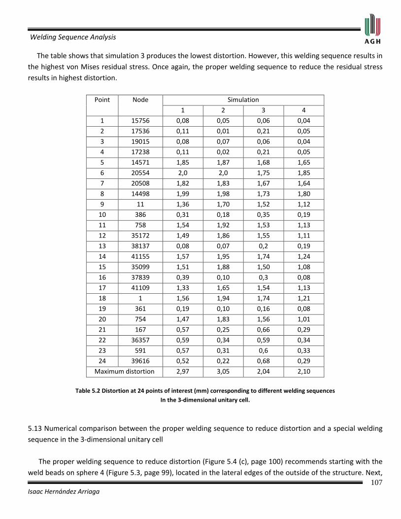
Welding Sequence Analysis
107 Isaac Hernández Arriaga
The table shows that simulation 3 produces the lowest distortion. However, this welding sequence results in the highest von Mises residual stress. Once again, the proper welding sequence to reduce the residual stress results in highest distortion.
Point Node Simulation
1 2 3 4
1 15756 0,08 0,05 0,06 0,04
2 17536 0,11 0,01 0,21 0,05
3 19015 0,08 0,07 0,06 0,04
4 17238 0,11 0,02 0,21 0,05
5 14571 1,85 1,87 1,68 1,65
6 20554 2,0 2,0 1,75 1,85
7 20508 1,82 1,83 1,67 1,64
8 14498 1,99 1,98 1,73 1,80
9 11 1,36 1,70 1,52 1,12
10 386 0,31 0,18 0,35 0,19
11 758 1,54 1,92 1,53 1,13
12 35172 1,49 1,86 1,55 1,11
13 38137 0,08 0,07 0,2 0,19
14 41155 1,57 1,95 1,74 1,24
15 35099 1,51 1,88 1,50 1,08
16 37839 0,39 0,10 0,3 0,08
17 41109 1,33 1,65 1,54 1,13
18 1 1,56 1,94 1,74 1,21
19 361 0,19 0,10 0,16 0,08
20 754 1,47 1,83 1,56 1,01
21 167 0,57 0,25 0,66 0,29
22 36357 0,59 0,34 0,59 0,34
23 591 0,57 0,31 0,6 0,33
24 39616 0,52 0,22 0,68 0,29
Maximum distortion 2,97 3,05 2,04 2,10
Table 5.2 Distortion at 24 points of interest (mm) corresponding to different welding sequences In the 3-dimensional unitary cell.
5.13 Numerical comparison between the proper welding sequence to reduce distortion and a special welding sequence in the 3-dimensional unitary cell The proper welding sequence to reduce distortion (Figure 5.4 (c), page 100) recommends starting with the weld beads on sphere 4 (Figure 5.3, page 99), located in the lateral edges of the outside of the structure. Next,
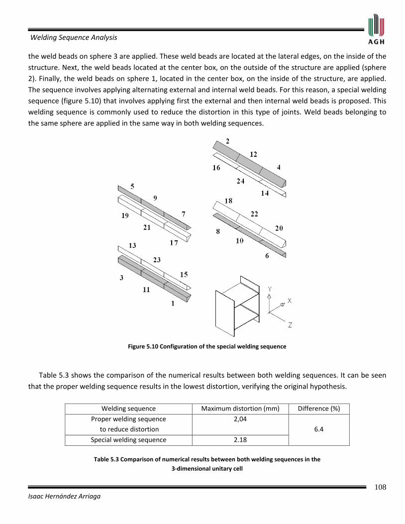
Welding Sequence Analysis
108 Isaac Hernández Arriaga
the weld beads on sphere 3 are applied. These weld beads are located at the lateral edges, on the inside of the structure. Next, the weld beads located at the center box, on the outside of the structure are applied (sphere 2). Finally, the weld beads on sphere 1, located in the center box, on the inside of the structure, are applied. The sequence involves applying alternating external and internal weld beads. For this reason, a special welding sequence (figure 5.10) that involves applying first the external and then internal weld beads is proposed. This welding sequence is commonly used to reduce the distortion in this type of joints. Weld beads belonging to the same sphere are applied in the same way in both welding sequences.
Figure 5.10 Configuration of the special welding sequence
Table 5.3 shows the comparison of the numerical results between both welding sequences. It can be seen that the proper welding sequence results in the lowest distortion, verifying the original hypothesis.
Welding sequence Maximum distortion (mm) Difference (%)
Proper welding sequence to reduce distortion
2,04 6.4
Special welding sequence 2.18
Table 5.3 Comparison of numerical results between both welding sequences in the 3-dimensional unitary cell

Welding Sequence Analysis
109 Isaac Hernández Arriaga
5.14 Conclusions of the welding sequence analysis of the 3-dimensional unitary cell
• Numerical simulations using 24 weld beads reduce distortion by up to 31% and residual stress by up to 18% with respect to numerical simulations using 8 weld beads.
• Numerical simulations of the proper welding sequence to reduce residual stress confirm the hypothesis in Section 5.2 by delivering minimum stress.
• Numerical simulations of the welding sequence to reduce distortion also confirm the hypothesis proposed in Section 5.2 by producing minimum distortion
• It has been demonstrated that the hypothesis to determine the proper welding sequences for flat symmetrical structures is also valid for symmetrical 3-dimensional structures.

Welding Sequence Analysis
110 Isaac Hernández Arriaga
CHAPTER VI
METHODOLOGY OF
EXPERIMENTAL TESTS 6.1 Introduction This chapter presents a methodology for helping plan, execute, and control each of the stages of the experimental tests. The methodology starts with the material selection of the specimen, configuration selection, welding process selection, metal transfer mode selection, welding parameters selection, design and fabrication of the equipment needed to run the test, design and fabrication of the mounting locks, residual stresses relief caused by the manufacturing process, transportation, handling, storage and cutting of the plates, measurement of the initial distortion of the plates, design and fabrication of a holder-mounting device to hold the plates, design and fabrication of a square-mounting device to square the holder-mounting device, application of welding tacks, measurement of the distortion after applying the welding tacks, installation of the run-off tabs, welding, removal of the run-off tabs of the welded structure, measurement of the distortion after welding, and measurement of the final distortion induced by the welding process. 6.2 Specimen material selection The specimen material is of great importance because it determines the selection of the welding process, parameters and material [35]. For this experiment, structural steel S235JR is selected. This steel is widely used in Europe (Poland: steel ST3S) for construction of ships, buildings, bridges and machinery [36]. This steel is easy to weld because of its carbon content (0.22% C), and its chemical composition, mechanical and thermal

Welding Sequence Analysis
111 Isaac Hernández Arriaga
properties are similar to ASTM A36 structural steel. Steel S235JR is therefore modeled using properties of ASTM A36 structural steel. 6.3 Selection of specimen configuration The configuration of the specimen determines the joint geometries, mounting configuration and the devices needed to adapt the components of the welding equipment. For this experiment a "three-dimensional unitary cell" configuration is selected because of its common applicability in industry for construction of panels, ships and bridges. The three-dimensional unitary cell consists of two horizontal and two vertical plates joined by fillet welds (figure 5.2, page 98). The thickness of the plates is 3 mm. 6.4 Selection of the welding process The appropriate selection of the welding process will produce an efficient application of the welding in the specimen. To produce the correct application, it is necessary to control the welding parameters, direction, and position of the welding torch. This implies that the selected welding process has to be semiautomatic or automatic. For this experiment, the Gas Metal Arc Welding (GMAW) process is selected because it can be automated. Furthermore, the welding laboratory of the Machine Strength and Manufacturing Department at the University of Sciences and Technology AGH, where the experiment took place, has a semiautomatic, OPTYMAG 501, welding machine (Figure 6.1, page 112). This machine is equipped with a microprocessor-controlled electrode wire feeder PDE-5, to fully adjust all of the welding process parameters (continuously indicated in a multifunctional LCD display). It also has an MG-2 gas mixer and a RTU-10-300 rotameter with a computerized system for process monitoring. The OPTYMAG 501 welding machine enables welding processes with the following methods: MIG/MAG standard, MIG/MAG pulse/synergic and manual mode and a MMA method for welding processes with coated electrodes. 6.5 Selection of metal transfer mode The operating features of the welding process are largely determined by the form in which the weld metal transfer takes place from the electrode to the weld pool [37]. The main metal transfer modes are: short circuiting transfer, globular transfer, spray transfer, and pulsed transfer. For this experiment we select short circuiting transfer for low current operation with small electrode diameters leading to a small, fast-cooling weld pool that is generally well suited for joining thin sections. In short circuiting transfer mode, also called “dip” transfer, the molten metal formed on the tip of the electrode wire is transferred by the wire dipping into the molten weld pool, thus causing a momentary short circuit. Metal is therefore transferred only when the electrode tip is in contact with the weld pool, and no metal is transferred across the arc gap.

Welding Sequence Analysis
112 Isaac Hernández Arriaga
Figure 6.1 Semiautomatic welding machine OPTYMAG 501
6.6 Selection of welding parameters (Operating variables) The weld geometry, depth of penetration, and overall quality of the weld process depends on the welding parameters [38]. These parameters are determined from the welding process, metal transfer mode, base metal, metal thickness and joint geometries. These parameters are: arc voltage, welding current, welding speed, wire feed rate, contact tip to work distance, electrode orientation, electrode diameter, shielding gas composition, and gas flow rate. 6.6.1 Arc voltage and welding current The arc voltage and welding current depend mainly on the metal transfer mode and the diameter of the electrode. According to Rao [39], the ranges of voltage and current recommended for different electrode
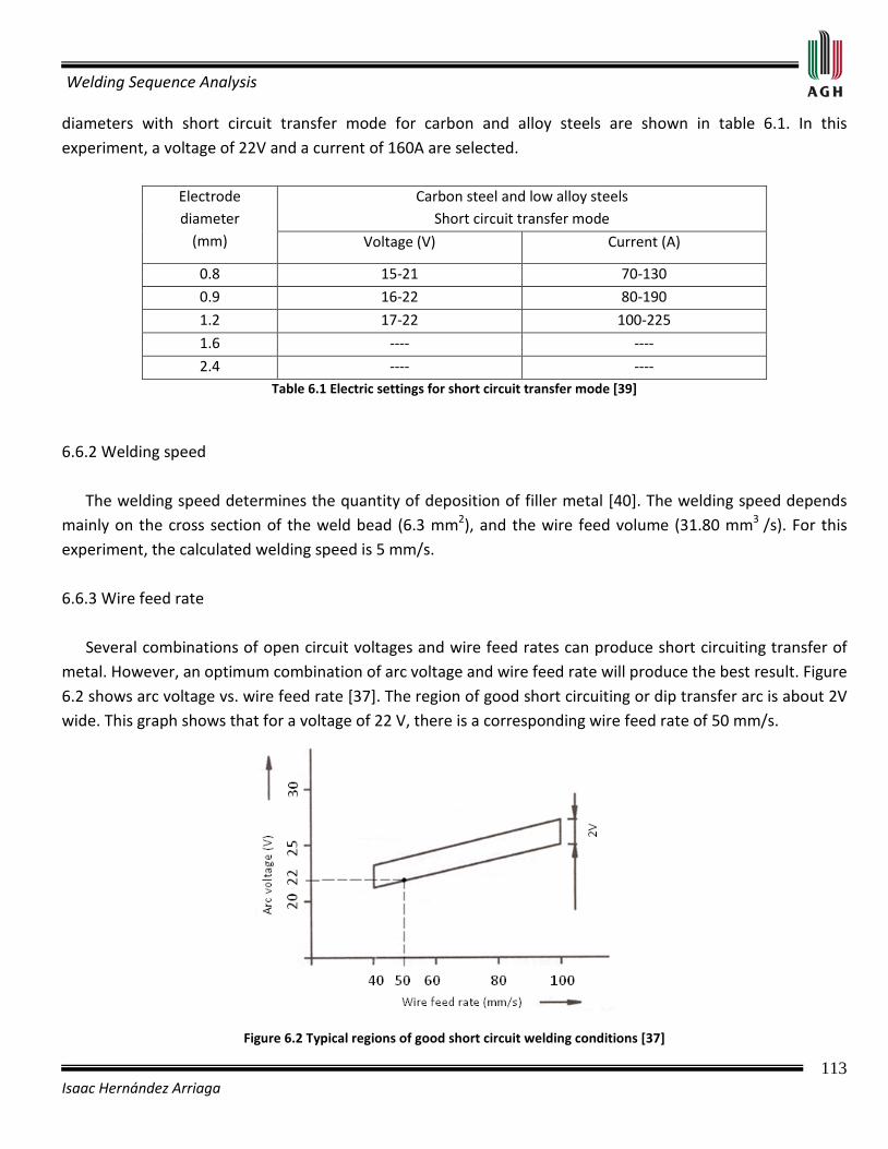
Welding Sequence Analysis
113 Isaac Hernández Arriaga
diameters with short circuit transfer mode for carbon and alloy steels are shown in table 6.1. In this experiment, a voltage of 22V and a current of 160A are selected.
Electrode diameter
(mm)
Carbon steel and low alloy steels Short circuit transfer mode
Voltage (V) Current (A)
0.8 15-21 70-130
0.9 16-22 80-190
1.2 17-22 100-225
1.6 ---- ----
2.4 ---- ---- Table 6.1 Electric settings for short circuit transfer mode [39]
6.6.2 Welding speed The welding speed determines the quantity of deposition of filler metal [40]. The welding speed depends mainly on the cross section of the weld bead (6.3 mm2), and the wire feed volume (31.80 mm3
Figure 6.2 Typical regions of good short circuit welding conditions [37]
/s). For this experiment, the calculated welding speed is 5 mm/s. 6.6.3 Wire feed rate Several combinations of open circuit voltages and wire feed rates can produce short circuiting transfer of metal. However, an optimum combination of arc voltage and wire feed rate will produce the best result. Figure 6.2 shows arc voltage vs. wire feed rate [37]. The region of good short circuiting or dip transfer arc is about 2V wide. This graph shows that for a voltage of 22 V, there is a corresponding wire feed rate of 50 mm/s.

Welding Sequence Analysis
114 Isaac Hernández Arriaga
6.6.4 Selecting of contact tip to work distance The contact tip to work distance (CTWD, Figure 6.3) determines the arc efficiency [40]. According to the Lincoln Electric Company, for short circuiting metal transfer mode, the CTWD should be held between 10 and 12 mm. For this experimental investigation, the selected CTWD is 11 mm.
Figure 6.3 Contact tip to work distance [40] 6.6.5 Electrode orientation The electrode orientation with respect to the weld joint affects the weld bead shape as well as the weld penetration. According to Mandal [37], the electrode orientation is defined in two ways:
• By the electrode axis orientation with respect to the direction of travel. This is known as the travel angle. The three possible ways to positioning the welding gun (figure 6.4), are called forehand, perpendicular and backhand. In this experimental investigation, the perpendicular positioning of the electrode gun with respect to the base metal plate is selected.
Figure 6.4. Positioning of electrode gun with respect to the base metal plate [37]

Welding Sequence Analysis
115 Isaac Hernández Arriaga
• The angle between the electrode axis and the adjacent work surface. This is called work angle. For fillet welds in the horizontal position, the electrode should be positioned at about 45° to the vertical plane (figure 6.5).
Figure 6.5 Normal work angle for fillet welds [37]
6.6.6 Electrode diameter The appropriate diameter of the electrode depends on the base metal composition, metal thickness, and the metal transfer mode [38]. In this experiment, the base material is carbon steel with a thickness of 3mm, and the metal transfer mode is by short circuit. Therefore, according to the AWS, the electrode diameter should be 0,9 mm. 6.6.7 Shielding gas composition The primary function of the shielding gas is to protect the arc and the molten weld pool from the atmospheric oxygen and nitrogen. The selection of the shielding gas composition depends on the base material and the metal transfer mode [39]. According to the Lincoln Electric Company, there are two common blends of shielding gases for short circuit transfer mode for carbon steels (Table 6.2). The blend 80% Argon + 20%CO2
Common short circuiting transfer shielding gas blends
is selected for this investigation.
75% Argon + 25%CO2- reduces spatter and improves weld bead appearance in carbon steel applications.
80% Argon + 20%CO2- Another popular blend, which further reduces spatter and enhances weld bead appearance in carbon steel applications.
Table 6.2 Common blends of shielding gas composition for short transfer mode [40]
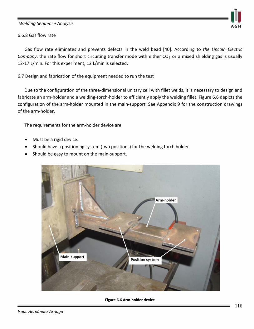
Welding Sequence Analysis
116 Isaac Hernández Arriaga
6.6.8 Gas flow rate Gas flow rate eliminates and prevents defects in the weld bead [40]. According to the Lincoln Electric Company, the rate flow for short circuiting transfer mode with either CO2
• Must be a rigid device.
or a mixed shielding gas is usually 12-17 L/min. For this experiment, 12 L/min is selected.
6.7 Design and fabrication of the equipment needed to run the test Due to the configuration of the three-dimensional unitary cell with fillet welds, it is necessary to design and fabricate an arm-holder and a welding-torch-holder to efficiently apply the welding fillet. Figure 6.6 depicts the configuration of the arm-holder mounted in the main-support. See Appendix 9 for the construction drawings of the arm-holder. The requirements for the arm-holder device are:
• Should have a positioning system (two positions) for the welding torch holder.
• Should be easy to mount on the main-support.
Figure 6.6 Arm-holder device

Welding Sequence Analysis
117 Isaac Hernández Arriaga
The requirements for the welding-torch-holder device are:
• Must have a rigid arm.
• Must have a system to rotate the welding torch from one position to another 90° apart.
• Must have a system to perform a zig-zag rotary motion for the welding torch.
• Should be easy to mount and remove on the arm-holder. Figure 6.7 depicts the configuration of the welding torch holder device. See Appendix 9 for the construction drawings of the welding torch holder device.
Figure 6.7 Welding torch holder device
6.8 Design and fabrication of the mounting locks The mounting locks position the specimen with respect to a reference point. The locks constrain the specimen in the X, Y and Z-directions. Figure 6.8 depicts the localization of the mounting locks on the traveler carriage.
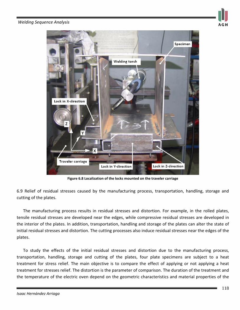
Welding Sequence Analysis
118 Isaac Hernández Arriaga
Figure 6.8 Localization of the locks mounted on the traveler carriage
6.9 Relief of residual stresses caused by the manufacturing process, transportation, handling, storage and cutting of the plates. The manufacturing process results in residual stresses and distortion. For example, in the rolled plates, tensile residual stresses are developed near the edges, while compressive residual stresses are developed in the interior of the plates. In addition, transportation, handling and storage of the plates can alter the state of initial residual stresses and distortion. The cutting processes also induce residual stresses near the edges of the plates. To study the effects of the initial residual stresses and distortion due to the manufacturing process, transportation, handling, storage and cutting of the plates, four plate specimens are subject to a heat treatment for stress relief. The main objective is to compare the effect of applying or not applying a heat treatment for stresses relief. The distortion is the parameter of comparison. The duration of the treatment and the temperature of the electric oven depend on the geometric characteristics and material properties of the

Welding Sequence Analysis
119 Isaac Hernández Arriaga
plates. For the present study, the heating time is 5 Hrs at 250 °C. Figure 6.9 depicts the electric oven used to relief the initial residual stresses.
Figure 6.9 Electric oven used to initial residual stresses relief
6.10 Measurement of the initial plate distortion It is important to measure the initial distortion of the plates to avoid errors in the measurements of distortion after welding, because, in many cases, the distortion due to the manufacturing process, transportation, handling, storage and cutting of the plates is larger than the distortion induced by the welding process. A series of standard gages are used to measure the initial distortion on a polished table. These standard gages have a minimum precision of 0.05 mm. Figure 6.10 depicts the measurement of the initial distortion on a polished table with standard gages.
Figure 6.10 Measurement of the initial distortion with standard gages
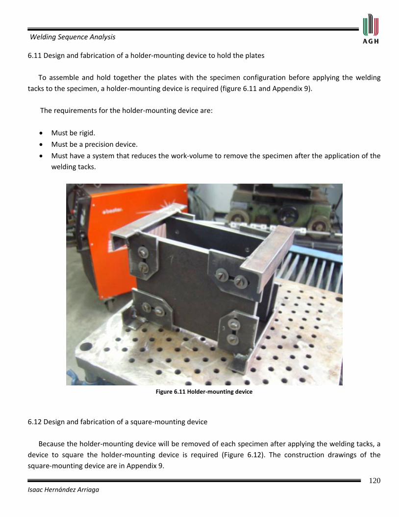
Welding Sequence Analysis
120 Isaac Hernández Arriaga
6.11 Design and fabrication of a holder-mounting device to hold the plates To assemble and hold together the plates with the specimen configuration before applying the welding tacks to the specimen, a holder-mounting device is required (figure 6.11 and Appendix 9). The requirements for the holder-mounting device are:
• Must be rigid.
• Must be a precision device.
• Must have a system that reduces the work-volume to remove the specimen after the application of the welding tacks.
Figure 6.11 Holder-mounting device
6.12 Design and fabrication of a square-mounting device Because the holder-mounting device will be removed of each specimen after applying the welding tacks, a device to square the holder-mounting device is required (Figure 6.12). The construction drawings of the square-mounting device are in Appendix 9.
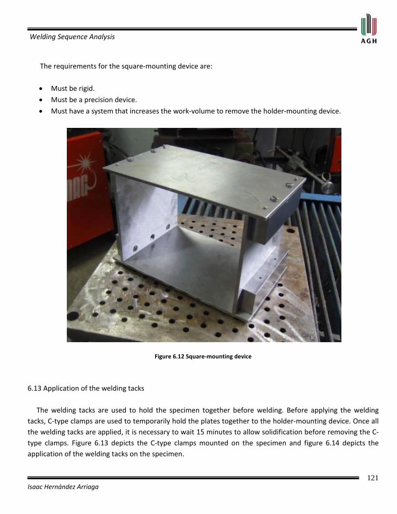
Welding Sequence Analysis
121 Isaac Hernández Arriaga
The requirements for the square-mounting device are:
• Must be rigid.
• Must be a precision device.
• Must have a system that increases the work-volume to remove the holder-mounting device.
Figure 6.12 Square-mounting device
6.13 Application of the welding tacks The welding tacks are used to hold the specimen together before welding. Before applying the welding tacks, C-type clamps are used to temporarily hold the plates together to the holder-mounting device. Once all the welding tacks are applied, it is necessary to wait 15 minutes to allow solidification before removing the C-type clamps. Figure 6.13 depicts the C-type clamps mounted on the specimen and figure 6.14 depicts the application of the welding tacks on the specimen.

Welding Sequence Analysis
122 Isaac Hernández Arriaga
Figure 6.13 C-type clamps mounted on the specimen
Figure 6.14 Welding tack application on the specimen
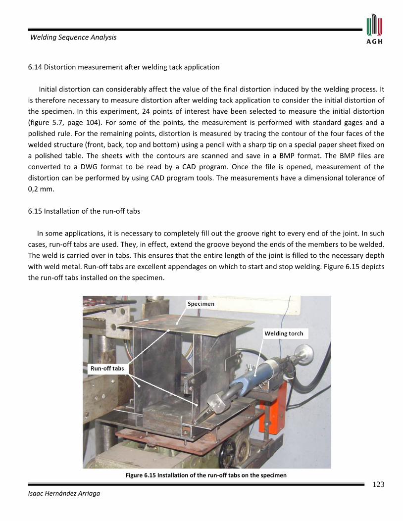
Welding Sequence Analysis
123 Isaac Hernández Arriaga
6.14 Distortion measurement after welding tack application Initial distortion can considerably affect the value of the final distortion induced by the welding process. It is therefore necessary to measure distortion after welding tack application to consider the initial distortion of the specimen. In this experiment, 24 points of interest have been selected to measure the initial distortion (figure 5.7, page 104). For some of the points, the measurement is performed with standard gages and a polished rule. For the remaining points, distortion is measured by tracing the contour of the four faces of the welded structure (front, back, top and bottom) using a pencil with a sharp tip on a special paper sheet fixed on a polished table. The sheets with the contours are scanned and save in a BMP format. The BMP files are converted to a DWG format to be read by a CAD program. Once the file is opened, measurement of the distortion can be performed by using CAD program tools. The measurements have a dimensional tolerance of 0,2 mm. 6.15 Installation of the run-off tabs In some applications, it is necessary to completely fill out the groove right to every end of the joint. In such cases, run-off tabs are used. They, in effect, extend the groove beyond the ends of the members to be welded. The weld is carried over in tabs. This ensures that the entire length of the joint is filled to the necessary depth with weld metal. Run-off tabs are excellent appendages on which to start and stop welding. Figure 6.15 depicts the run-off tabs installed on the specimen.
Figure 6.15 Installation of the run-off tabs on the specimen

Welding Sequence Analysis
124 Isaac Hernández Arriaga
6.16 Application of the welding The application of the welding is made by following a sequence. The selection of the welding sequence depends on the critical parameter or parameters to reduce – residual stress, distortion or a relation between both. Chapters 4 and 5 described the proper welding sequences to reduce residual stress, distortion or a relation between both for symmetrical structures in 2 and 3 dimensions. For this experiment, we selected the welding sequence to reduce residual stress and distortion for symmetrical structures in the space. Figure 6.16 depicts the specimen welding.
Figure 6.16 Application of the welding to the specimen
6.17 Removing the run-off tabs from the welded structure The run-off tabs should be removed to be able to perform the distortion measurements. These run-off tabs are removed once the welding process is completed. Care must be taken when removing them to not induce residual stresses, or distortion, or both. First the run-off tab material close to the specimen is removed. This can be performed with an abrasive disc. Then, each of the run-off tabs is removed, and at the end, the irregular edges are taken out with a grinder. Figure 6.17 depicts the removal of the run-off tabs from the specimen.
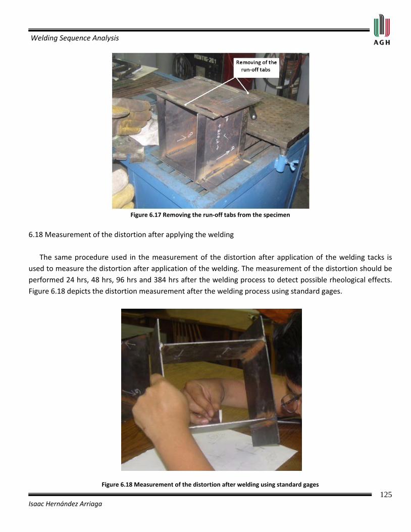
Welding Sequence Analysis
125 Isaac Hernández Arriaga
Figure 6.17 Removing the run-off tabs from the specimen
6.18 Measurement of the distortion after applying the welding The same procedure used in the measurement of the distortion after application of the welding tacks is used to measure the distortion after application of the welding. The measurement of the distortion should be performed 24 hrs, 48 hrs, 96 hrs and 384 hrs after the welding process to detect possible rheological effects. Figure 6.18 depicts the distortion measurement after the welding process using standard gages.
Figure 6.18 Measurement of the distortion after welding using standard gages
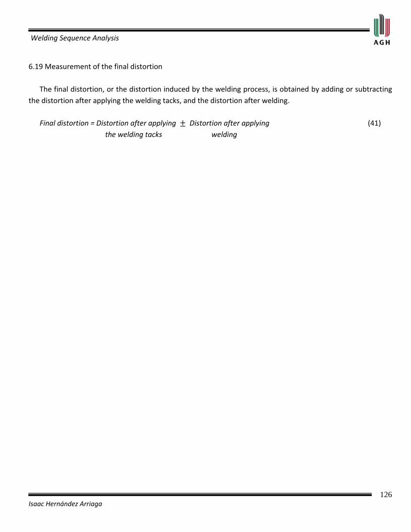
Welding Sequence Analysis
126 Isaac Hernández Arriaga
6.19 Measurement of the final distortion The final distortion, or the distortion induced by the welding process, is obtained by adding or subtracting the distortion after applying the welding tacks, and the distortion after welding. Final distortion = Distortion after applying Distortion after applying (41) the welding tacks welding
Welding Sequence Analysis
127 Isaac Hernández Arriaga
CHAPTER VII
RESULTS OF THE EXPERIMENTAL TESTS IN 3-DIMENSIONAL UNITARY CELL-TYPE
SPECIMENS 7.1 Introduction This chapter covers the results of the experimental tests performed in 3-dimensional unitary cell specimens. In these experimental tests, the effects of the welding sequence on distortion are studied. Eight symmetrical specimens are prepared. Four welding sequences are considered: two of them are appropriate to reduce distortion and the others are appropriate to reduce residual stresses. Also, the effects that occur when a welding bead is divided into 3 sub-weld beads are studied, as well as the effects of relieving the residual stresses caused by manufacturing process, transportation, storage and cutting of plates. Welding tacks are applied to all specimens before the actual weld process begins. The measurement of the distortion is periodically performed to observe if rheological effects occur in the specimens after welding. The experimental tests were performed in the Department of Machine Strength and Manufacturing in the Faculty of Mechanical Engineering at the University of Science and Technology in Krakow, Poland. 7.2 Configuration of the 3-dimensional unitary cell specimens The 3-dimensional unitary cell specimens have the same configuration analyzed in Chapter 5. The main objective of using the same configuration is performing a quantitative and qualitative comparison between
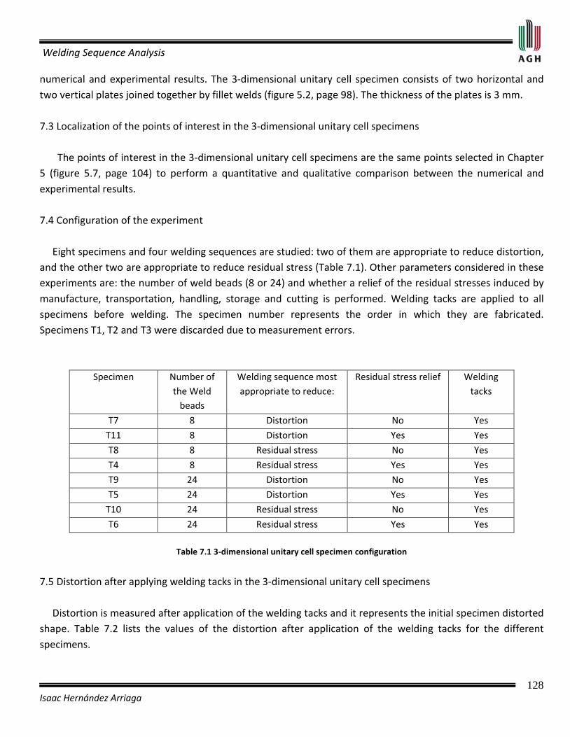
Welding Sequence Analysis
128 Isaac Hernández Arriaga
numerical and experimental results. The 3-dimensional unitary cell specimen consists of two horizontal and two vertical plates joined together by fillet welds (figure 5.2, page 98). The thickness of the plates is 3 mm. 7.3 Localization of the points of interest in the 3-dimensional unitary cell specimens The points of interest in the 3-dimensional unitary cell specimens are the same points selected in Chapter 5 (figure 5.7, page 104) to perform a quantitative and qualitative comparison between the numerical and experimental results. 7.4 Configuration of the experiment Eight specimens and four welding sequences are studied: two of them are appropriate to reduce distortion, and the other two are appropriate to reduce residual stress (Table 7.1). Other parameters considered in these experiments are: the number of weld beads (8 or 24) and whether a relief of the residual stresses induced by manufacture, transportation, handling, storage and cutting is performed. Welding tacks are applied to all specimens before welding. The specimen number represents the order in which they are fabricated. Specimens T1, T2 and T3 were discarded due to measurement errors.
Specimen Number of the Weld
beads
Welding sequence most appropriate to reduce:
Residual stress relief Welding tacks
T7 8 Distortion No Yes
T11 8 Distortion Yes Yes
T8 8 Residual stress No Yes
T4 8 Residual stress Yes Yes
T9 24 Distortion No Yes
T5 24 Distortion Yes Yes
T10 24 Residual stress No Yes
T6 24 Residual stress Yes Yes
Table 7.1 3-dimensional unitary cell specimen configuration
7.5 Distortion after applying welding tacks in the 3-dimensional unitary cell specimens Distortion is measured after application of the welding tacks and it represents the initial specimen distorted shape. Table 7.2 lists the values of the distortion after application of the welding tacks for the different specimens.

Welding Sequence Analysis
129 Isaac Hernández Arriaga
Point Specimen
T7 T11 T8 T4 T9 T5 T10 T6
1 0,15 0,55 0,25 0,10 0,40 0,20 0,20 0,30
2 0,15 0,20 0,25 0,30 0,10 0,05 0,20 0,20
3 0,25 0,05 0,2 0,15 0,15 0,20 0,10 0,10
4 0,20 0,20 0,05 0,35 0,15 0,10 0 0,05
5 0,95 0,60 0,25 0,93 0,5 0,55 0,55 0,75
6 0,65 0,38 0,60 1,15 0,43 0,95 0,35 0,93
7 0,93 0,60 0,63 1,43 0,80 0,60 0,80 0,45
8 0,92 0,63 0,28 1,38 0,15 0,58 0,45 0,80
9 (-) 1,10 (-) 1,00 (-) 0,40 (-) 1,70 (-) 1,15 (-) 0,45 (-) 0,30 (-) 0,70
10 (-) 0,15 (-) 0,25 0,10 0,10 0 (-) 0,20 0,25 0,25
11 (-) 0,10 (-) 0,20 (-) 0,10 (-) 1,25 (-) 0,70 (-) 0,50 (-) 0,15 (-) 0,20
12 (-) 0,20 (-) 0,35 0 (-) 0,95 (-) 0,30 (-) 0,55 (-) 0,60 (-) 0,30
13 (-) 0,05 (-) 0,15 (-) 0,05 0,05 0 0,20 0,05 0,20
14 (-) 0,40 (-) 0,45 (-) 1,10 (-) 1,10 (-) 0,55 (-) 1,20 0,30 (-) 1,25
15 (-) 0,85 (-) 0,65 (-) 0,45 (-) 1,45 (-) 0,10 (-) 0,25 0 (-) 0,55
16 (-) 0,10 0,35 0,45 0 (-) 0,15 (-) 0,20 0,35 0,15
17 (-) 0,50 0,30 (-) 0,35 (-) 0,95 (-) 0,50 (-) 0,25 (-) 0,60 (-) 0,20
18 (-) 0,20 (-) 0,10 (-) 0,20 (-) 1,50 (-) 0,60 (-) 0,90 (-) 0,30 (-) 0,65
19 0,25 0,05 0,15 0,10 0,25 (-) 0,10 0,50 0,35
20 (-) 0,65 (-) 1,00 (-) 0,70 (-) 1,80 (-) 0,80 (-) 1,05 (-) 1,10 (-) 0,80
21 (-) 0,50 (-) 0,25 (-) 0,05 (-) 0,05 (-) 0,15 (-) 0,40 0,15 0
22 (-) 0,45 (-) 0,30 (-) 0,05 (-) 0,10 (-) 0,30 (-) 0,35 (-) 0,10 (-) 0,10
23 (-) 0,20 (-) 0,35 0,05 (-) 0,10 (-) 0,20 (-) 0,25 0 0
24 (-) 0,40 (-) 0,35 0,15 0,05 (-) 0,20 (-) 0,25 (-) 0,15 0
Table 7.2 Distortion after application of the welding tacks for the different 3-dimensional unitary cell specimens, mm.
7.6 Distortion after welding in the 3-dimensional unitary cell specimens Distortion is measured after welding and it represents the final distorted specimen shape. It is necessary to note that these measurements do not represent the distortion induced by the welding process because the specimens were originally distorted by the application of the welding tacks.
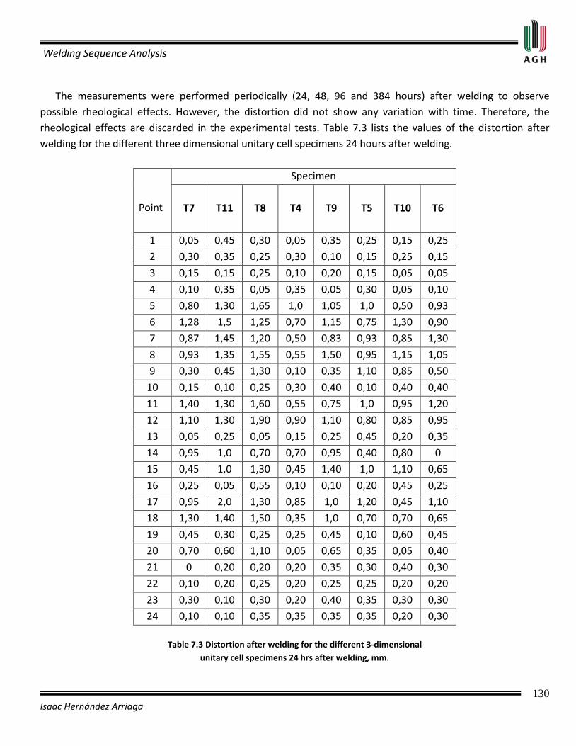
Welding Sequence Analysis
130 Isaac Hernández Arriaga
The measurements were performed periodically (24, 48, 96 and 384 hours) after welding to observe possible rheological effects. However, the distortion did not show any variation with time. Therefore, the rheological effects are discarded in the experimental tests. Table 7.3 lists the values of the distortion after welding for the different three dimensional unitary cell specimens 24 hours after welding.
Point
Specimen
T7
T11
T8
T4
T9
T5
T10
T6
1 0,05 0,45 0,30 0,05 0,35 0,25 0,15 0,25
2 0,30 0,35 0,25 0,30 0,10 0,15 0,25 0,15
3 0,15 0,15 0,25 0,10 0,20 0,15 0,05 0,05
4 0,10 0,35 0,05 0,35 0,05 0,30 0,05 0,10
5 0,80 1,30 1,65 1,0 1,05 1,0 0,50 0,93
6 1,28 1,5 1,25 0,70 1,15 0,75 1,30 0,90
7 0,87 1,45 1,20 0,50 0,83 0,93 0,85 1,30
8 0,93 1,35 1,55 0,55 1,50 0,95 1,15 1,05
9 0,30 0,45 1,30 0,10 0,35 1,10 0,85 0,50
10 0,15 0,10 0,25 0,30 0,40 0,10 0,40 0,40
11 1,40 1,30 1,60 0,55 0,75 1,0 0,95 1,20
12 1,10 1,30 1,90 0,90 1,10 0,80 0,85 0,95
13 0,05 0,25 0,05 0,15 0,25 0,45 0,20 0,35
14 0,95 1,0 0,70 0,70 0,95 0,40 0,80 0
15 0,45 1,0 1,30 0,45 1,40 1,0 1,10 0,65
16 0,25 0,05 0,55 0,10 0,10 0,20 0,45 0,25
17 0,95 2,0 1,30 0,85 1,0 1,20 0,45 1,10
18 1,30 1,40 1,50 0,35 1,0 0,70 0,70 0,65
19 0,45 0,30 0,25 0,25 0,45 0,10 0,60 0,45
20 0,70 0,60 1,10 0,05 0,65 0,35 0,05 0,40
21 0 0,20 0,20 0,20 0,35 0,30 0,40 0,30
22 0,10 0,20 0,25 0,20 0,25 0,25 0,20 0,20
23 0,30 0,10 0,30 0,20 0,40 0,35 0,30 0,30
24 0,10 0,10 0,35 0,35 0,35 0,35 0,20 0,30
Table 7.3 Distortion after welding for the different 3-dimensional unitary cell specimens 24 hrs after welding, mm.

Welding Sequence Analysis
131 Isaac Hernández Arriaga
Figure 7.1 shows a comparison between the distortion after applying welding tacks and the distortion after welding for specimen T9, illustrating the distorted shape before and after welding.
Figure 7.1 Distortion (exaggerated) after applying welding tacks and after
welding for specimen T9

Welding Sequence Analysis
132 Isaac Hernández Arriaga
7.7 Distortion modes of the 3-dimensional unitary specimens All welded specimens present the same distortion mode. However, the magnitude of the distortion varies. The lower and upper flanges rotate inward to the specimen, and the plates of the central box bend toward the center of the specimen (Figure 7.2).
Figure 7.2 Distorted shape of the 3-dimensional unitary cell welded specimens
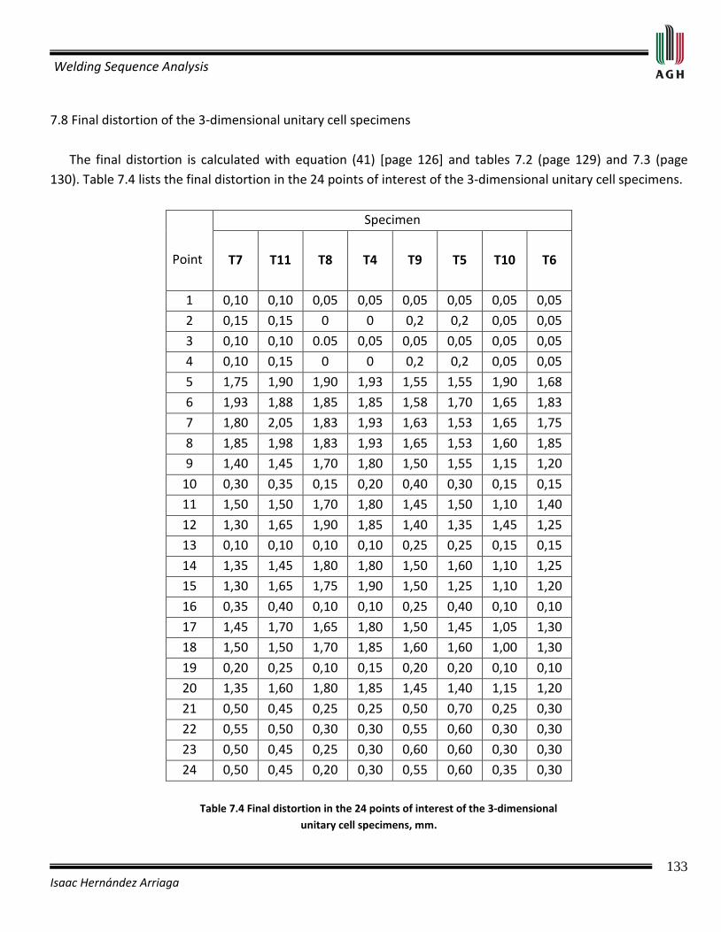
Welding Sequence Analysis
133 Isaac Hernández Arriaga
7.8 Final distortion of the 3-dimensional unitary cell specimens The final distortion is calculated with equation (41) [page 126] and tables 7.2 (page 129) and 7.3 (page 130). Table 7.4 lists the final distortion in the 24 points of interest of the 3-dimensional unitary cell specimens.
Point
Specimen
T7
T11
T8
T4
T9
T5
T10
T6
1 0,10 0,10 0,05 0,05 0,05 0,05 0,05 0,05
2 0,15 0,15 0 0 0,2 0,2 0,05 0,05
3 0,10 0,10 0.05 0,05 0,05 0,05 0,05 0,05
4 0,10 0,15 0 0 0,2 0,2 0,05 0,05
5 1,75 1,90 1,90 1,93 1,55 1,55 1,90 1,68
6 1,93 1,88 1,85 1,85 1,58 1,70 1,65 1,83
7 1,80 2,05 1,83 1,93 1,63 1,53 1,65 1,75
8 1,85 1,98 1,83 1,93 1,65 1,53 1,60 1,85
9 1,40 1,45 1,70 1,80 1,50 1,55 1,15 1,20
10 0,30 0,35 0,15 0,20 0,40 0,30 0,15 0,15
11 1,50 1,50 1,70 1,80 1,45 1,50 1,10 1,40
12 1,30 1,65 1,90 1,85 1,40 1,35 1,45 1,25
13 0,10 0,10 0,10 0,10 0,25 0,25 0,15 0,15
14 1,35 1,45 1,80 1,80 1,50 1,60 1,10 1,25
15 1,30 1,65 1,75 1,90 1,50 1,25 1,10 1,20
16 0,35 0,40 0,10 0,10 0,25 0,40 0,10 0,10
17 1,45 1,70 1,65 1,80 1,50 1,45 1,05 1,30
18 1,50 1,50 1,70 1,85 1,60 1,60 1,00 1,30
19 0,20 0,25 0,10 0,15 0,20 0,20 0,10 0,10
20 1,35 1,60 1,80 1,85 1,45 1,40 1,15 1,20
21 0,50 0,45 0,25 0,25 0,50 0,70 0,25 0,30
22 0,55 0,50 0,30 0,30 0,55 0,60 0,30 0,30
23 0,50 0,45 0,25 0,30 0,60 0,60 0,30 0,30
24 0,50 0,45 0,20 0,30 0,55 0,60 0,35 0,30
Table 7.4 Final distortion in the 24 points of interest of the 3-dimensional
unitary cell specimens, mm.
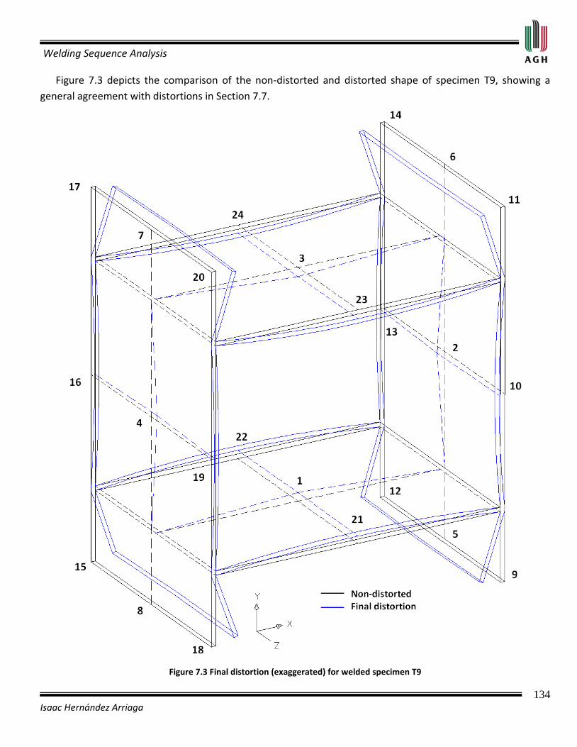
Welding Sequence Analysis
134 Isaac Hernández Arriaga
Figure 7.3 depicts the comparison of the non-distorted and distorted shape of specimen T9, showing a general agreement with distortions in Section 7.7.
Figure 7.3 Final distortion (exaggerated) for welded specimen T9

Welding Sequence Analysis
135 Isaac Hernández Arriaga
7.9 Final Remarks for distortion of the 3-dimensional unitary cell specimens For the points located at the center of the plates (points 1, 2, 3 and 4):
• There is symmetry with respect to the horizontal (points 1 and 3) and vertical (points 2 and 4) axes.
• Welding with 24 beads results in higher distortion than welding with 8 beads.
• When following a welding sequence from the outside to the inside of the structure, specimens with 8 weld beads develop higher distortion.
• Little variation is observed between welded specimens with or without stress-relief. For points 5, 6, 7 and 8 located at the central part of the lower and upper flanges:
• Specimens with 8 weld beads result in higher distortion than specimens with 24 weld beads.
• Welded specimens with stress-relieved plates develop a slight increase in distortion.
• Specimens welded with 24 weld beads that use a sequence from the outside to the inside of the structure developed less distortion than specimens using the opposite sequence. In specimens welded with 8 weld beads no significant trend was identified.
For points 9, 11, 12, 14, 15, 17, 18 and 20 located at the edges of the lower and upper flanges:
• There is no distortion symmetry in any axis.
• Specimens with 8 weld beads show higher distortion than specimens with 24 beads.
• Welded specimens with stress-relieved plates develop higher distortion than specimens without stress-relief.
• In 8 bead specimens, following a welding sequence from the outside to the inside of the structure produces less distortion than using the converse sequence. However, 24 bead specimens using an inside-to-outside sequence developed less distortion than specimens using the converse sequence.
For points 10, 13, 16 and 19 located at the central part of the lateral edges of the vertical plates:
• Welding sequences starting from the inside to the outside of the structure developed less distortion than specimens using the opposite welding sequence.
• Distortion is slightly higher in the specimens welded with 24 beads.
• Little difference is observed between specimens with and without stress-relieved plates.
Welding Sequence Analysis
136 Isaac Hernández Arriaga
For points 21, 22, 23 and 24 located at the central part of the lateral edges of the horizontal plates:
• Specimens welded with 24 beads develop higher distortion than specimens with 8 weld beads.
• Specimens without stress-relief develop higher distortion than specimens with stress-relievef.
7.10 Conclusions of the results of the experimental test in 3-dimensional unitary cell specimens
• In all welded specimens, the maximum distortion occurs at the central part of the lower and upper flanges (points 5, 6, 7 and 8).
• The specimens with 8 weld beads show higher distortion than specimens with 24 weld beads.
• Little difference is observed between specimens with or without stress-relieved plates.
• Specimens with 24 beads following a welding sequence starting from the outside to the inside of the structure, show the lowest distortion without taking into account the stress-relief in the plates.
Welding Sequence Analysis
137 Isaac Hernández Arriaga
CHAPTER VIII
COMPARISON BETWEEN THE
3- DIMENSIONAL UNITARY CELL-TYPE STRUCTURES/SPECIMENS
8.1 Introduction This chapter presents a comparison between numerical (Chapter 5) and experimental (Chapter 7) results for the 3-dimensional unitary cell structure. The comparison discusses the distortion modes, and distortion in the 24 points of interest. The end of this chapter presents the procedures to determine the proper welding sequences to reduce the residual stresses, distortion, or a relation between them in symmetrical and asymmetrical structures in 2 and 3 dimensions. These procedures are based on the demonstrated hypotheses developed in Chapters 4 and 5. 8.2 Comparison of distortion modes The distortion modes of all the numerical simulations (figure 5.9, page 106) agree with the experimental results (figure 7.2, page 132). The lower and upper flanges rotate inward towards the specimen, and the central area of the flange bends towards the specimen. The central areas of the vertical and horizontal plates bend inward to the structure. 8.3 Comparison of distortion Numerical distortion at the 24 points of interest (table 5.2, page 107) can be directly compared with the experimental results (table 7.4, page 133). It is important to mention that the numerical simulations do not consider relief of the initial residual stresses. For this reason, only four numerical simulations were developed vs. eight experiments. Therefore, each of the simulations will be compared against two experiments: with or

Welding Sequence Analysis
138 Isaac Hernández Arriaga
without stress relief. Equation 42 is used to determine the percentage difference between numerical and experimental results for each of the 24 points of interest:
(42)
Table 8.1 depicts the difference percentage between numerical and experimental results.
Point Specimen
T7
T11
T8
T4
T9
T5
T10
T6
1 20 20 0 0 -20 -20 20 20
2 26,6 26,6 --- --- -5 -5 0 0
3 20 20 -40 -40 -20 -20 20 20
4 -10 26,6 --- ---- -5 -5 0 0
5 -5,7 2,6 1,6 3,1 -8,4 -8,4 13,1 1,8
6 -3,6 -6.4 -8,1 -8,1 -10,7 -2,9 -12,2 -1,1
7 -1,1 11,2 0 5,2 -2,4 -9,1 0,6 6,3
8 -7.5 -0,5 -8.2 -2.6 -4,8 -13 -12,5 2,7
9 2,8 6,2 0 5,5 -1,3 1,9 2,6 6,6
10 -3,3 11,4 -20 10 12,5 -16,6 -26,6 -26,6
11 -2,6 -2,6 -12,9 -6,6 -5,5 -2 -2,7 19,3
12 -14,6 9,7 2,1 -0,5 -10,7 -13,3 23,4 11,2
13 20 20 30 30 20 20 -26,6 -26,6
14 14 -8,2 -8,3 -8,3 -16 -8,7 -12,7 0,8
15 -16,2 8,5 -7.4 1 0 -20 1,8 10
16 -11,4 2,5 0 0 -20 25 20 20
17 8,2 21,7 0 8,3 -2,6 -6,2 -7,6 13
18 -4 -4 -14,1 -4,8 -8,7 -8,7 -21 6,9
19 5 24 0 33 20 20 20 20
20 -8,8 8,1 -1,6 1,1 -7,6 -11,4 12,1 15,8
21 -14 -26.6 0 0 -32 5,7 -16 3,3
22 -7,2 -18 -13,3 -13,3 -7,2 1,6 -13,3 -13,3
23 -14 -26.6 -24 -3,3 0 0 -10 -10
24 -4 -15,5 -10 26,6 -23.6 -13,3 17,1 3,3
Table 8.1 Difference (%) between numerical and experimental results
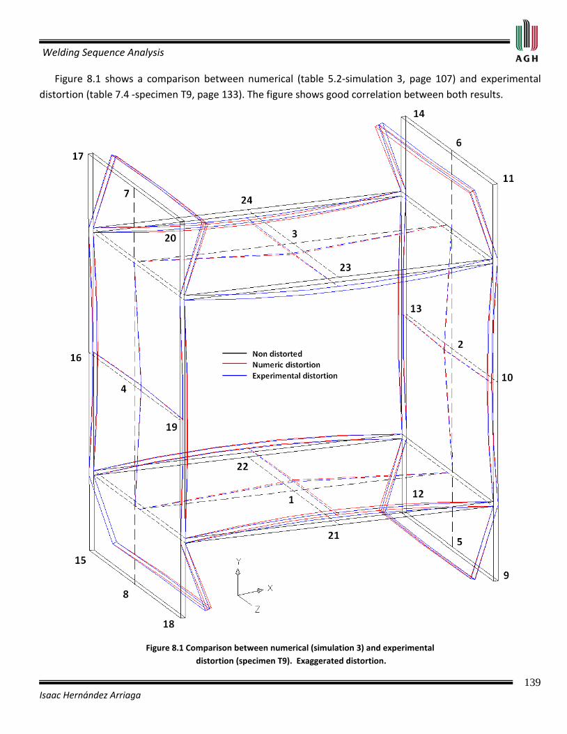
Welding Sequence Analysis
139 Isaac Hernández Arriaga
Figure 8.1 shows a comparison between numerical (table 5.2-simulation 3, page 107) and experimental distortion (table 7.4 -specimen T9, page 133). The figure shows good correlation between both results.
Figure 8.1 Comparison between numerical (simulation 3) and experimental
distortion (specimen T9). Exaggerated distortion.

Welding Sequence Analysis
140 Isaac Hernández Arriaga
8.4 Conclusions of the comparison between numerical and experimental results
• Of the 192 points of interest, 17 points show a good correlation in distortion between numerical and experimental results, 87 points present a difference between 0,1-10%, 61 points differ by 10,1-20%, 17 points are different by 20,1-30%, 2 points present a difference between 30,1-40%, and 4 points cannot be compared. The resulting comparison is considered acceptable.
• Welded specimens without stress-relief present smaller differences than specimens fabricated with stress-relief, with the exception of specimen T10.
• The maximum differences in distortion occur in the points located at the center of the horizontal and vertical plates because the magnitude of the distortion in these points is very small. As an example, variations as small as 0,01 mm result in large percentage differences.
8.5 Procedures to determine the proper welding sequences to reduce residual stress, distortion, or a relation between them in symmetrical and asymmetrical structures in 2 and 3 dimensions Based on the demonstrated hypotheses to determine the proper welding sequence to reduce the residual stress, distortion, or a relationship between them in symmetrical structures in 2 (Chapter 4) and 3 dimensions (Chapter 5), the following procedures are obtained to determine proper welding sequences. Hypotheses for symmetrical structures are also adapted to asymmetrical structures. However, this hypothesis was not demonstrated. 8.5.1 Symmetrical structures in 2 and 3 dimensions To determine the proper welding sequence to reduce the residual stress, distortion, or a relation between them in symmetrical structures in the plane/space, the procedure is as follows: Determine the axis of symmetry and the center of gravity of the structure. Draw concentric circles/spheres centered on the center of gravity of the structure and extending to the center of gravity of each of the weld beads. The weld beads located at the same distance from the center of gravity of the structure fall on the same circle/sphere. The circles/spheres are numbered from the smallest to the largest. Procedure No.1- To reduce residual stress: Start with the weld beads on the smallest circle/sphere and then continue with the weld beads on the larger adjacent circle/sphere until the largest circle/sphere is reached. The weld beads on the same circle/sphere should be symmetrical. First, the weld beads with diagonal symmetry are selected. If the weld bead with diagonal symmetry has already been selected, then the farthest symmetrical weld bead is selected next. When a current weld bead has more than one farthest symmetrical weld bead, the adjacent weld bead in

Welding Sequence Analysis
141 Isaac Hernández Arriaga
counter-clockwise direction is selected. Finally, to move from one circle/sphere to the other, the farthest weld bead to the current weld bead is selected. If a current weld bead has more than one farthest weld bead, the adjacent weld bead in counter-clockwise direction is selected. The converse welding method between weld beads is adopted. Procedure No.2- To reduce distortion: Apply welding tacks to the structure before welding. First, the weld beads in the largest circle/sphere are selected, followed by the weld beads on the adjacent smaller circle/sphere, until the smallest circle/sphere is reached. The application of the weld beads on the same circle/sphere should be in symmetrical form. The weld beads with diagonal symmetry are selected first. If the weld bead with diagonal symmetry has already been selected, then the farthest symmetrical weld bead is selected next. When a current weld bead has more than one farthest symmetrical weld bead, the adjacent weld bead in counter-clockwise direction is selected next. Finally, to move from one circle/sphere to the other, the farthest weld bead to the current is selected. If a current weld bead has more than one farthest weld bead, the adjacent weld bead in a clockwise direction is selected. The converse welding method between weld beads is adopted. Procedure No.3- To improve the residual stress-distortion relation while prioritizing the reduction in residual stresses: First, the weld beads on the smallest circle/sphere are selected and then continuing with the weld beads on the larger adjacent circle/sphere until the largest circle/sphere is reached. The application of weld beads on the same circle/sphere should be in an adjacent form in counter-clockwise direction. To move from one circle/sphere to the other, the closest weld bead to the current is selected. The converse welding method between weld beads is adopted. Procedure No.4- To improve the residual stress-distortion relation while prioritizing the reduction of distortion: Welding tacks are required only on the circle/sphere next to the larger adjacent circle/sphere. The welding sequence begins by selecting the weld beads on the smallest circle/sphere, and then continuing with the weld beads on the circle/sphere next to the larger adjacent circle/sphere. Then, going back to the weld beads on the smaller adjacent circle/sphere. The application of the weld beads on the same circle/sphere should be in a symmetrical form. First, the weld beads with diagonal symmetry are applied. If the weld bead with diagonal symmetrical has already been applied, then the farthest symmetrical weld bead is selected. When a current weld bead has more than one farthest symmetrical weld bead, the adjacent weld bead in counter-clockwise direction is selected. Finally, to move from one circle/sphere to the other, the farthest weld bead is selected
Welding Sequence Analysis
142 Isaac Hernández Arriaga
next. If a current weld bead has more than one farthest weld bead, the adjacent weld bead in counter-clockwise direction is selected. The converse welding method between weld beads is adopted. 8.5.2 Asymmetrical structures in 2 and 3 dimensions The procedure to determine the proper welding sequence to reduce the residual stress, distortion, or a relation between them in asymmetrical structures is as follows: Find the center of gravity of the structure and draw concentric circles/spheres centered on the center of gravity of the structure and extending to the center of gravity of each of the weld beads. The weld beads that are located at the same distance from the center of gravity of the structure will fall on the same circle/sphere. The circles/spheres are numbered from the smallest to the largest. Procedure No.5- To reduce the residual stress: First, the weld beads on the smallest circle/sphere are selected and then continuing with the weld beads on the adjacent larger circle/sphere until the largest circle/sphere. Next, the farthest weld bead to the current weld bead on the same circle/sphere is selected. When a current weld bead has more than one farthest weld bead in the same circle/sphere, the adjacent weld bead in counter-clockwise direction is selected. Finally, to move from one circle/sphere to the other, the farthest weld bead to the current weld bead is selected. If a current weld bead has more than one farthest weld bead, the adjacent weld bead in counter-clockwise direction is selected. The converse welding method is adopted between weld beads. Procedure No.6- To reduce the distortion: Apply welding tacks to the structure. First, the weld beads belonging to the largest circle/sphere are selected and then the weld beads belonging to the adjacent smaller circle/sphere, until the smallest circle/sphere is reached. Next, the farthest weld bead to the current weld bead on the same circle/sphere is selected. When a current weld bead has more than one farthest weld bead in the same circle/sphere, the adjacent weld bead in counter-clockwise direction is selected. Finally, to move from one circle/sphere to the other, the farthest weld bead to the current is selected. If a current weld bead has more than one farthest weld bead, the adjacent weld bead in a clockwise direction is selected. The converse welding method is adopted between weld beads. Procedure No.7- To improve the residual stress-distortion relation while prioritizing the reduction of residual stresses. First, the weld beads on the smallest circle/sphere are selected, and then continuing with the weld beads on the larger adjacent circle/sphere until the largest circle/sphere is reached. The application of the weld
Welding Sequence Analysis
143 Isaac Hernández Arriaga
beads on the same circle/sphere should be in an adjacent form in counter-clockwise direction. Finally, to move from one circle/sphere to the other, the closest weld bead to the current weld bead is selected. The converse welding method is adopted between weld beads. Procedure No.8- To improve the residual stress-distortion relation while prioritizing the reduction of distortion: The application of welding tacks is required only on the circle/sphere next to the larger adjacent circle/sphere. The welding sequence begins by selecting the weld beads on the smallest circle/sphere, and then continuing with the weld beads on the circle/sphere next to the larger adjacent circle/sphere. Then, going back to the weld beads on the smaller adjacent circle/sphere. Next, the farthest weld bead to the current weld bead on the same circle/sphere is applied. When a current weld bead has more than one farthest weld bead, the adjacent weld bead in counter-clockwise direction is selected next. Finally, to move from one circle/sphere to the other, the farthest weld bead to the current weld bead is selected next. If a current weld bead has more than one farthest weld bead, the adjacent weld bead in counter-clockwise direction is selected. The converse welding method is adopted between weld beads. Figure 8.2 depicts the flow diagram of the analysis of the welding sequence for symmetrical and asymmetrical structures in 2 and 3 dimensions. The main goal of this flow diagram is to facilitate reading by a welder, for determining the proper welding sequences to reduce the required critical parameter, and additionally, to be used by the weld-cognizant engineer in the design stage to check the welding sequences with a finite element code.

Welding sequence analysis
144 Isaac Hernández Arriaga
Figure 8.2 Flow Diagram of the analysis of the welding sequence for symmetrical and asymmetrical structures in 2 and 3 dimensions
Welding Sequence Analysis
145 Isaac Hernández Arriaga
CHAPTER IX
CONCLUSIONS, CONTRIBUTIONS, AND SUGGESTIONS FOR
FUTURE RESEARCH 9.1 Conclusions The following conclusions are limited to analyzed cases in this thesis:
• The maximum residual stress occurs in the base metal, at the boundary with the welded metal.
• Validation of the numerical simulation of the welding process vs. experimental results shows satisfactory results, with less than 8.3% difference.
• The welding sequence considerably affects the residual stresses and the distortion in welded structures.
• The welding sequence that produces the lowest distortion also produces the highest residual stress and vice versa.
• The welding sequence has a bigger effect on distortion than on residual stresses.
• The comparison between numerical results of the 3-dimensional unitary cell with experimental tests shows satisfactory results, with less than 40% difference.
• Dividing a weld bead in several sub-welds reduces distortion but increases residual stresses.
• Combining the welding sequence and converse welding method considerably reduces distortion and residual stresses.
• To reduce distortion it is necessary to apply welding tacks to the structure before welding begins.
• To reduce the residual stresses, welding tacks are not recommended.
• Application of the weld beads from the inside to the outside of the structure, without the use of welding tacks results in the lowest residual stress, but the highest distortion.
• Application of the weld beads from the outside to the inside of the structure, with the use of welding tacks, results in the lowest distortion, but in the highest residual stresses.
• Application of the weld beads from the inside to the outside of the structure with the use of welding tacks reduces distortion, but increases residual stress.

Welding Sequence Analysis
146 Isaac Hernández Arriaga
• Application of the weld beads from the outside to the inside of the structure without the use of welding tacks, reduces residual stresses, but increases distortion.
• The hypothesis to determine the proper welding sequences for 2-dimensional symmetrical structures is valid for 3-dimensional symmetrical structures.
9.2 Contributions
• A finite element-based simulation of the welding process. A sequentially coupled thermo-mechanical analysis is proposed. A transient heat transfer analysis is first performed, followed by a thermo elasto-plastic analysis. The material is assumed to follow the von Mises yield criterion and the associated flow rule, lineal isotropic hardening, and the temperature-dependent thermal and mechanical properties of the selected material. The micro-structural evolution is not considered
• A comparison of the numerical simulation of the welding process to experimental tests.
• A study of the effects of the welding sequence on the residual stress and distortion on particular symmetrical structures in 2 and 3 dimensions.
• A residual stress-distortion relation analysis due to the welding sequence for 2-dimensional symmetrical structures.
• An equation to determine the residual stress-distortion relation:
• A hypothesis to determine the proper welding sequence to reduce the residual stress, distortion or a
relation between them for 2-dimensional symmetrical structures (Chapter 4, Section 4.9).
• A hypothesis to determine the proper welding sequence to reduce the residual stress, distortion or a relation between them, for 3-dimensional symmetrical structures (Chapter 5, Section 5.2).
• Validation of the hypotheses to determine the proper welding sequence to reduce the residual stress, distortion or a relation between them, for symmetrical structures in 2 and 3 dimensions.
• Procedures to select the proper welding sequence to reduce the residual stress, distortion, or a relation between them for symmetrical structures in 2 and 3 dimensions.
• Development of a methodology to perform experimental tests.
• Experimental comparison of the proper welding sequences to reduce the distortion and/or the residual stress in a 3-dimensional symmetrical structure.
9.3 Suggestion for future research
• Include the effects of micro-structural evolution in the numerical simulation of the welding process.
• Measurement of the residual stress in the 3-dimensional unitary cell specimens.
Welding Sequence Analysis
147 Isaac Hernández Arriaga
• Application of this methodology to determine the proper welding sequence to reduce the residual stress, distortion or a relation between them, for other common structures in the welding industry. Appendix 4 proposes some welding sequences to reduce the residual stresses and distortion in common symmetrical structures. These welding sequences have not been numerically verified.
• Develop a family-group classification of the symmetrical structures in 2 and 3 dimensions to determine the proper welding sequence to reduce the residual stress, distortion or a relation between them.
• Develop a computer program to automatically determine the proper welding sequences to reduce residual stress, distortion or a relation between them, for symmetrical structures in 2 and 3 dimensions.
• Develop a methodology to determine the proper welding sequence to reduce the residual stress, distortion or a relation between them for asymmetrical structures.
Welding Sequence Analysis
148 Isaac Hernández Arriaga
REFERENCES
[1] Zhili, F., 2005, “Processes and Mechanisms of Welding Residual Stress and Distortion”, CRC Press. [2] Masubuchi, K., 1980, “Analysis of Welded Structures: Residual Stresses, Distortion, and their
Consequences”, Pergamon Press. [3] Masubuchi, K., 2001, “Welding Handbook: Residual Stress and Distortion”, American Welding Society,
9th
[4] edition.
Messler, R., 1999, “Principles of Welding: Processes, Physics, Chemistry, and Metallurgy”, John Wiley and Sons, Inc.
[5] Murugan, V., Gunaraj, V., 2005, “Effects of Process parameters on angular distortion of gas metal arc welded structural steel plates”, Weld. J. 84 (11): 165s-171s.
[6] Tso-Liang Teng., Ching-Cheng Lin., 1998, “Effect of welding condition on residual stress due to butt welds”, Int. J. Pressure Vessels and Piping, 75: 857-864.
[7] Jang, B., Kim, H. K., Kang S., 2001, “Effects of root opening on mechanical properties, deformation and residual stress of weldments”, Weld. J. 80 (7): 80s-88s.
[8] Bhide, S. R., Michaleris, P., Posada, M., Deloach, J., 2006, “Comparison of buckling distortion propensity for SAW, GMAW, y FSW”, Weld. J. 85 (9): 189s-195s.
[9] Wahab, M. A., Alam, M. S., Painter, M. J., Stafford, P. E., 2006, “Experimental and numerical simulation of restraining forces in gas metal arc welded joints”, Weld. J. 85 (2): 35s-43s.
[10] Muhammad, Abid., Muhammad, Siddique., 2005, “Numerical simulation of the effect of constraints on welding deformations and residual stresses in a pipe-flange joint”, Modeling Simul. Mater. Sci. Eng. 13: 919-933.
[11] Michaleris, P., Sun, X., 1997, “Finite Element Analysis of Thermal Tensioning Techniques Mitigating Weld Buckling Distortion”, Weld. J. 76(11): 451s-457s.
[12] Michaleris, P., Dantzig, J., Tortorelli, D., 1999, “Minimization of welding residual stress and distortion in large structures” Weld. J. 78 (11): 361-366.
[13] Holdren, R. L., Greer, J. E., 2001, “Welding Handbook: Terms and definition, Appendix A.”, American Welding Society, 9th
[14] edition,
The Lincoln Electric Company, 1933, “Procedure handbook of arc welding design and practice”, Cleveland, Ohio, U.S.A.
[15] Bart, O. N., Deepak, G., Kyoung, Y. K., 2004, “Welding distortion minimization for an aluminum alloy extruded beam structure using a 2D model”, ASME J. Manufacturing Science and Engineering, 126: 52-63.
[16] Tso, L. T., Peng, H. C., Wen, C. T., 2003, “Effect of welding sequence on residual stresses”, Computer and Structures, 81: 273-286.
[17] Ji, S. D., Fang, H. Y., Liu, X. S., Meng, Q. G., 2005, “Influence of a welding sequence on the welding residual stress of a thick plate”, Modeling and Simulation in Materials Science and Engineering, 13: 553-565.
Welding Sequence Analysis
149 Isaac Hernández Arriaga
[18] Nami, M. R., Kadivar, M. H., Jafarpur, K., 2004, “3D thermo-viscoplastic modeling of welds: Effect of
piece-wise welding on thermo-mechanical response of thick plate weldments”, Iranian Journal of Science and Technology, Transaction B, Vol. 28, No. B4, 467-478.
[19] Mochizuki, M., Hayashi, M., 2000, “Residual stress distribution depending on welding sequence in multi-pass welded joints with X-shaped groove”, ASME J. Pressure Vessel Technology. 122: 27-32.
[20] Mochizuki, M., Hattori, T., Nakakado, K., 2000 , “Residual stress reduction and fatigue strength improvement by controlling welding pass sequence”, ASME J. Engineering Materials and Technology, 122: 108-112.
[21] Tsai, C. L., Park, S. C., Cheng, W. T., 1999, “Welding distortion of a thin-plate panel structure”, Weld. J. 78 (11): 156s-165s.
[22] Hackmair, C., Werner, E., Pönisch, M., 2003, “Application of welding simulation for chassis components within the development of manufacturing methods”, Computational materials Science, 28: 540-547.
[23] Kadivar, M. H., Jafarpur, K., Baradaran, G. H., 2000, “Optimizing welding sequence with genetic algorithm”, Computational Mechanics. 26: 514-519.
[24] Voutchkov, I., Keane, A. J., Bhaskar, A., Olsen, T. M., 2005, “Weld sequence optimization: the use of surrogate models for solving sequential combinatorial problems”, Computer methods in applied mechanics and engineering, 194: 3535-3551.
[25] Hernández, A. I., 2005, “Análisis de distorsión y esfuerzos residuales en estructuras soldadas”, Tesis de maestría, Universidad de Guanajuato.
[26] Karlsson, L., 1986, “Thermal Stresses I-Chapter 5: Thermal Stresses in welding”, Edited by Hetnarski R. B., Elsevier Science Publishers B.V.
[27] Argyris, J. H., Szimmat, J., William, K. J., 1982, “Computational aspect of welding stress analysis”, Computer methods in applied mechanics and engineering, 33: 635-666.
[28] Boley, B., Weiner, J., 1962, “Theory of thermal stresses”, John Wiley and Sons, Second Edition. [29] Goldak, J.A., Akhlaghi Mehdi., 2005, “Computational Welding Mechanics”, Springer. [30] Cook, R., Malkus, D., Plesha, M., Witt, R., 2002, “Concepts and Application of Finite Element Analysis”,
John Wiley and Sons, Fourth Edition. [31] Doghri, I., 2000, “Mechanics of Deformable Solid: Linear and Nonlinear, Analytical and Computational
Aspects”, Springer. [32] Malvern, L., 1969, “Introduction to the Mechanics of a Continuous Medium”, Prentice Hall, Inc. [33] William, D., Callister, Jr., 2000, “Materials Science and Engineering an Introduction”, John Wiley and
Sons, inc. Fifth Edition. [34] Chang, P. H., 2003, “Numerical and experimental investigation on residual stresses of the butt-welded
joints”, Computation Material Science, 29: 511-522. [35] Tso-Liang Teng., Ching-Cheng Lin., Peng-Hsiang Chang., 2002, “Effect of weld geometry and residual
stresses on fatigue in butt-welded joints”, Int. J. Pressure Vessels and Piping, 79: 467-482. [36] Pilarczyk, J., 2003, “Poradnik inżyniera Spawalnictwo część 1”, Wydawnictwa Naukowo-Techniczne,
Polska. (In polish) [37] Mandal, N. R., 2004, “Welding and distortion control”, Alpha Science International Ltd. [38] Holdren, R. L., Greer, J. E., 2001, “Welding Handbook: Volume 2.”, American Welding Society, 9th
[39]
edition, Rao, P. N., 2001, “Manufacturing Technology: Foundry, Forming and Welding”, McGraw-Hill International, Second Edition.
Welding Sequence Analysis
150 Isaac Hernández Arriaga
[40] Nadzam, J., 2006, “Gas Metal Arc Welding Guidelines”, The Lincoln Electric Company, Cleveland, Ohio, U.S.A.
[41] Słuzalec, A., 2005, “Theory of Thermomechanical Processes in Welding”, Springer. [42] Prat, P., Gens, A., 2000, “Leyes de comportamiento de materiales” Métodos Numéricos para Cálculo y
Diseño en Ingeniería, Barcelona. [43] Simo, J., Hugnes T., 1998, “Computational Inelasticity”, Interdisciplinary Applied Mathematics, Vol. 7,
Springer-Verlag, New York, Inc. [44] Makhnenko, V. I., Veliokoivanenko, E. A., 1999, “Numerical Methods for the Predictions of welding
stresses and distortions”, E. O. Paton Electric Welding Institute, Volume 13, Part 1. [45] Nicholson, D., 2003, “Finite Element Analysis: Thermomechanics of Solid”, CRC Press. [46] Klaus-Jurgen Bathe, 1996, “Finite Element Procedures”, Prentice Hall. [47] Swanson Analysis Systems, Inc. “ANSYS user´s manual: Elements”, Vol. III.
Welding Sequence Analysis
151 Isaac Hernández Arriaga
APPENDIX 1
Welding Sequence Analysis
152 Isaac Hernández Arriaga
Plasticity theory applied to welding process and its formulation by finite element method 1. Plasticity theory applied to welding process Plasticity-based analysis provides an engineering basis for study of residual stress and distortion [1]. The
temperature of the metal in welds varies from melting temperature ( )mT to room temperature ( )ambT . The
domain includes the liquid weld pool and the far field of solid near room temperature. The material´s behavior depends on the temperature range encountered in the different regions in the weld. At temperatures above 0.8 mT , the solid can be considered to be linear viscous. Between 0.5 and 0.8 mT , the material is rate
dependent. For 0.5 mT , the solid can be considered to be viscoplastic and characterized by an elasticity tensor,
viscosity and deformation resistance. Below 0.5 mT , the solid can be considered to be rate independent plastic
material characterized by an elasticity tensor, yield strength and isotropic hardening modulus [29]. Most thermal stress analyses have used thermal elastic plastic constitutive models with rate independent plasticity. Rate independent plasticity implies zero viscosity and therefore zero relaxation time. This means the stress relaxes instantly to the yield stress. A rate independent model is certainly not valid in the liquid region and is suspected near the melting point where the viscous effects are expected to be important [29]. Furthermore, the mechanical and thermal properties of weld and base metal are dependent on temperature [1,29,41]. 2. Mathematical considerations in the modeling of the welding process Welding process simulation considers small displacements [2,41]. Therefore, the infinitesimal strain is defined as:
( ), ,
12ij i j j iu uε = + (43)
The strain in equation (43) is known as the Cauchy strain tensor. Changes in stress caused by deformation are also assumed to travel slowly compared to the speed of sound. So, at any instant, an observed group of material particles is approximately in static equilibrium [1]: , 0ij j ifσ + = (19)
Where: if is the sum of the body force and ijσ is the Cauchy stress tensor.
To ensure that the body remains continuous during the deformation, the compatibility equations must be satisfied [2]. , , , , 0ij kl kl ij ik jl jl ikε ε ε ε+ − − = (20)

Welding Sequence Analysis
153 Isaac Hernández Arriaga
3. Rate independent isotropic plasticity in the modeling of the welding process Rate independent plasticity occurs at low temperatures, roughly below 0.5 mT . The deformation is due to
dislocation glide and strain rate due to fluctuations plays no significant role. The relaxation time is zero. In the simulation of the welding process it is important to assume the appropriate material behavior of the weld and base metal. The additive decomposition of strain, yield surface, flow rule and the hardening hypothesis should be assumed in such a way to describe the welding process as realistic as possible [41]. 3.1 Additive decomposition of total strain This section shows a derivation of the constitutive equations in differential (increment) form for thermal elastic plastic isotropic material, assuming that total strain increment can be decomposed (valid for small strains and small rotations) as [1]:
Tot e p trij ij ij ij ijd d d d dθε ε ε ε ε= + + + (44)
Where: eijdε is the elastic strain increment, p
ijdε is the plastic strain increment, ijd θε is the thermal strain
increment, and trijdε is the phase transformation strain increment. The metallurgical evolution may develop
stresses due to strain incompatibility during solid-state phase transformation. This strain incompatibility results in stresses between the grains of different phases, which may have a significant influence on the state of residual stresses in the weld metal and heat affected zone in joining certain types of materials such as martensitic weldments. However, this phase transformation stress is usually ineffective in influencing the final state of weld distortion. Equation (44) is therefore reduced to:
e pij ij ij ijd d d d θε ε ε ε= + + (21)
Equation (21) represents the additive decomposition of total strain increment considered in this investigation. Figure 1 depicts the decomposition of total strain into elastic, plastic and thermal.
Figure 1. Stress-strain curve of thermal elastic plastic material [42,43]
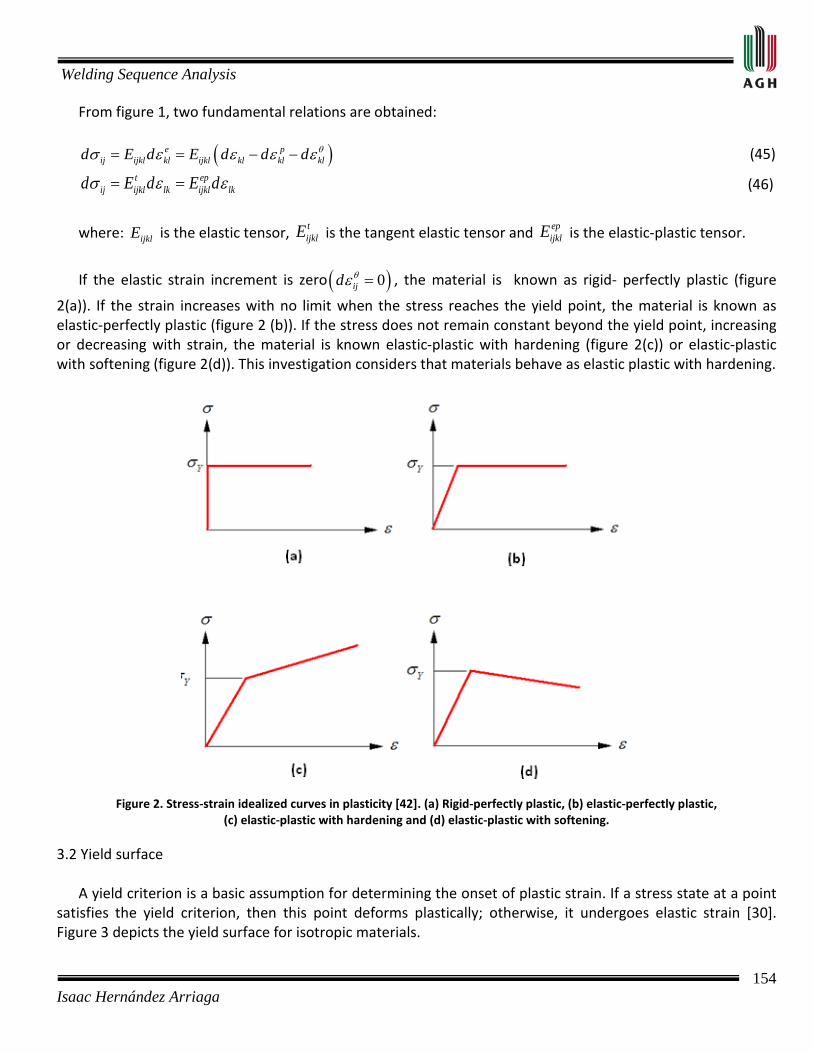
Welding Sequence Analysis
154 Isaac Hernández Arriaga
From figure 1, two fundamental relations are obtained: ( )e p
ij ijkl kl ijkl kl kl kld E d E d d d θσ ε ε ε ε= = − − (45)
t epij ijkl lk ijkl lkd E d E dσ ε ε= = (46)
where: ijklE is the elastic tensor, tijklE is the tangent elastic tensor and ep
ijklE is the elastic-plastic tensor.
If the elastic strain increment is zero ( )0ijd θε = , the material is known as rigid- perfectly plastic (figure
2(a)). If the strain increases with no limit when the stress reaches the yield point, the material is known as elastic-perfectly plastic (figure 2 (b)). If the stress does not remain constant beyond the yield point, increasing or decreasing with strain, the material is known elastic-plastic with hardening (figure 2(c)) or elastic-plastic with softening (figure 2(d)). This investigation considers that materials behave as elastic plastic with hardening.
Figure 2. Stress-strain idealized curves in plasticity [42]. (a) Rigid-perfectly plastic, (b) elastic-perfectly plastic,
(c) elastic-plastic with hardening and (d) elastic-plastic with softening. 3.2 Yield surface
A yield criterion is a basic assumption for determining the onset of plastic strain. If a stress state at a point satisfies the yield criterion, then this point deforms plastically; otherwise, it undergoes elastic strain [30]. Figure 3 depicts the yield surface for isotropic materials.

Welding Sequence Analysis
155 Isaac Hernández Arriaga
The general expression of the yield surface is written as [42]: ( ), 0ij if σ χ = (47)
where: iχ are parameters that control the yield surface size
Figure 3. Yield surface for isotropic materials [42]
Generalizing the different material behavior showed in figure 2, the yield surface becomes [42]:
• Perfect plasticity: the yield surface only depends on the magnitudes of the stress, not changed in size during the load process. In this case, equation (47) reduces to:
( ) 0ijf σ = (48)
• Rigid Plasticity: the yield surface expands during the load process.
• Soften Plasticity: the yield surface contracts during the load process. When the body is under plastic domain, the stress state should be on the yield surface. Thus, given a defined stress state ijσ and parameters, iχ , yields [42]:
( ), 0ij if σ χ < ⇒ for elastic deformation domain
( ), 0ij if σ χ = ⇒ for plastic deformation domain
( ), 0ij if σ χ > ⇒ impossible
For the general case of modeling of the welding process, the yield surface has the form [2]:
( )( ), , , 0p pij ijf Tσ ε κ ε = (49)
Where: κ is the parameter related with the strain hardening effects and T is the temperature.
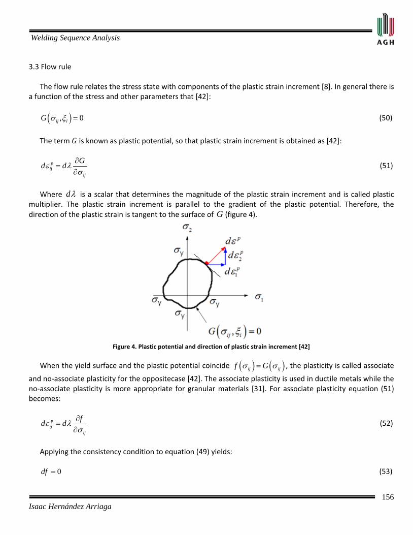
Welding Sequence Analysis
156 Isaac Hernández Arriaga
3.3 Flow rule The flow rule relates the stress state with components of the plastic strain increment [8]. In general there is a function of the stress and other parameters that [42]: ( ), 0ij iG σ ξ = (50)
The term is known as plastic potential, so that plastic strain increment is obtained as [42]:
pij
ij
Gd dε λσ∂
=∂
(51)
Where dλ is a scalar that determines the magnitude of the plastic strain increment and is called plastic multiplier. The plastic strain increment is parallel to the gradient of the plastic potential. Therefore, the direction of the plastic strain is tangent to the surface of G (figure 4).
Figure 4. Plastic potential and direction of plastic strain increment [42]
When the yield surface and the plastic potential coincide ( ) ( )ij ijf Gσ σ= , the plasticity is called associate
and no-associate plasticity for the oppositecase [42]. The associate plasticity is used in ductile metals while the no-associate plasticity is more appropriate for granular materials [31]. For associate plasticity equation (51) becomes:
pij
ij
fd dε λσ∂
=∂
(52)
Applying the consistency condition to equation (49) yields: 0df = (53)
Welding Sequence Analysis
157 Isaac Hernández Arriaga
0pij ijp
ij ij
f f f fd d d dTT
σ ε κσ ε κ∂ ∂ ∂ ∂
+ + + =∂ ∂ ∂ ∂
(54)
The consistency condition means that if yield occurs during a time interval, the solution should always remain on the yield surface [32].
Since pijp
ij
d dκκ εε∂
=∂
and the flow rule is pij
ij
fd dε λσ∂
=∂
, substituting these expressions into equation (54),
produces:
klkl
f fd Q d dTT
λ σσ
∂ ∂= + ∂ ∂
(55)
The plastic multiplier takes specific values to remain on the yield surface at all times: 0dλ = if 0f < (Elastic strain) 0dλ > if 0f = and 0df = (Yielding) 0dλ = if 0f = and 0df < (Unloading) If 0dλ > , the plastic strain increments are determined from the flow rule. If equation (55) is introduced into equation (51), the plastic strain increment becomes:
pij kl
ij kl ij
f f f fd Q d dTT
ε σσ σ σ
∂ ∂ ∂ ∂= + ∂ ∂ ∂ ∂
(56)
Where; 1
p pij ij ij
Qf f fκε κ ε σ
= − ∂ ∂ ∂ ∂
+ ∂ ∂ ∂ ∂
(57)
3.4 Hardening hypothesis The hardening hypothesis describes how the yield surface is modified by the plastic strain beyond the initial yield [8]. Under this hypothesis, the yield surface is not constant but may change in size, shape and/or position during the process of plastic strain [6]. There are three fundamental hardening hypotheses [30-33,42-43]: a) Null hardening. The hardening energy is absent in an ideally plastic material (perfect plasticity). The yield surface for this material is not changed by the presence of plastic strain as illustrated in figure 5 (a). If the stress state remains on the yield surface in the path 1-2, then the evolution of the plastic strain occurs, the path 2-3 corresponds to elastic unload.

Welding Sequence Analysis
158 Isaac Hernández Arriaga
b) Isotropic hardening. Assumes that the subsequent yield surface is a uniform expansion of the initial yield surface, as shown in figure 5(b), and that the material´s isotropic response to yielding remains unchanged during plastic strain. Thus the center of initial and subsequent yield surface is the same. In isotropic hardening, the variable κ depends on the plastic strain or plastic work.
For the case of strain hardening, ( )pF dκ ε= ∫ where pdε is the equivalent strain increment defined as:
23
p p pij ijd d dε ε ε= (58)
For the case of work hardening, ( )pF dWκ = ∫ where pdW is the work plastic increment defined as:
p pij ijdW dσ ε= (59)
c) Kinematic hardening. Assumes that the yield surface moves as a rigid body in the stress space during plastic strain. As a result the shape of the subsequent yield surface during plastic strain remains unchanged. This hardening is more appropriate for cyclic plasticity, because isotropic hardening cannot predict the Bauschingers effect which is observed experimentally [31]. For this investigation, isotropic strain hardening (Figure 5 (b)) is selected.
(a) (b) (c)
Figure 5. Three fundamental hypothesis of hardening [42]. (a) Null hardening, (b) isotropic hardening, and (c) kinematic hardening.
4. Von Mises model applied to the welding process Welding process simulation is based on two important considerations [1, 2, 26,27]: 1) Welding is for ductile metals (associate plasticity) and 2) Deformations occur without volume change (independent of the spherical
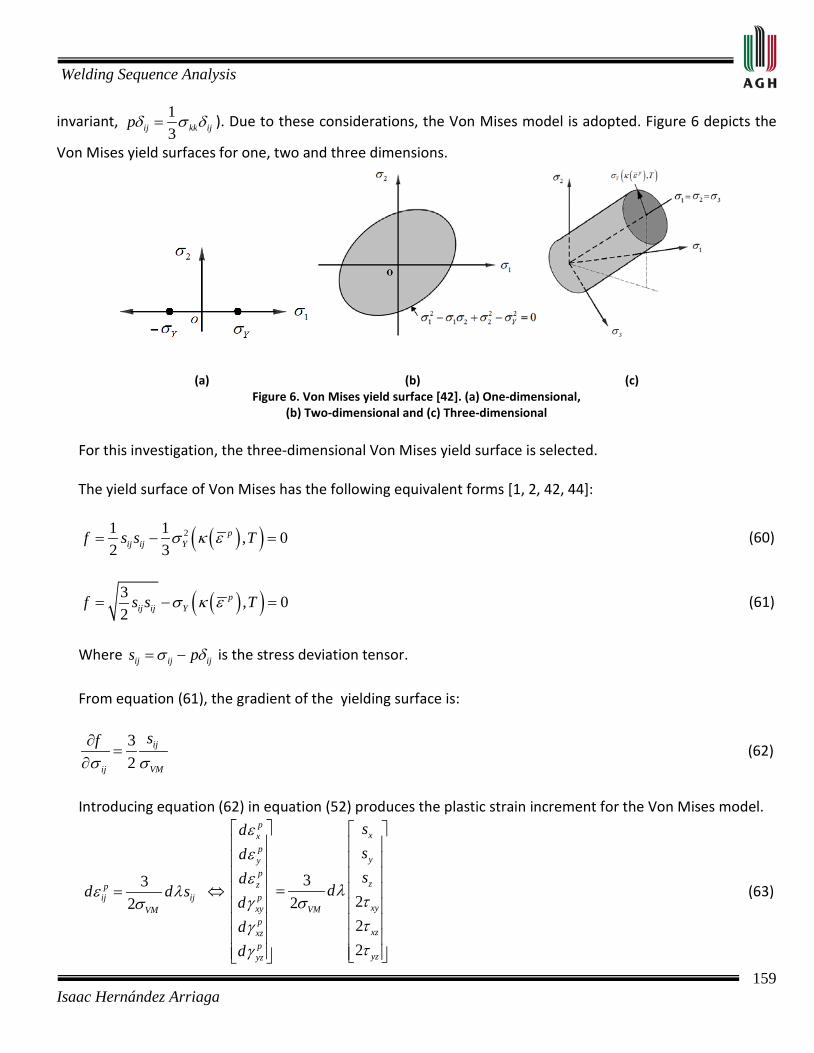
Welding Sequence Analysis
159 Isaac Hernández Arriaga
invariant, 13ij kk ijpδ σ δ= ). Due to these considerations, the Von Mises model is adopted. Figure 6 depicts the
Von Mises yield surfaces for one, two and three dimensions.
(a) (b) (c) Figure 6. Von Mises yield surface [42]. (a) One-dimensional,
(b) Two-dimensional and (c) Three-dimensional For this investigation, the three-dimensional Von Mises yield surface is selected. The yield surface of Von Mises has the following equivalent forms [1, 2, 42, 44]:
( )( )21 1 , 02 3
pij ij Yf s s Tσ κ ε= − = (60)
( )( )3 , 02
pij ij Yf s s Tσ κ ε= − = (61)
Where ij ij ijs pσ δ= − is the stress deviation tensor.
From equation (61), the gradient of the yielding surface is:
32
ij
ij VM
sfσ σ∂
=∂
(62)
Introducing equation (62) in equation (52) produces the plastic strain increment for the Von Mises model.
3
2p
ij ijVM
d d sε λσ
= ⇔3
2222
pxx
pyy
pzz
pxyxy VM
pxzxz
pyzyz
sdsdsd
dddd
εεε
λτγ στγτγ
=
(63)

Welding Sequence Analysis
160 Isaac Hernández Arriaga
and then, using equation (61), equation (57) becomes:
1
pij ij
Qf fε σ
= − ∂ ∂ ∂ ∂
(64)
In the Von Mises yield criterion, the plastic multiplier is equal to the equivalent strain increment [30-32, 42]: pd dλ ε= (65) Equation (65) into equation (52) becomes:
1p
pij ij
f εσ ε∂ ∂
=∂ ∂
(66)
Equation (66) into equation (64) becomes:
1 1 1
pij
pp pij
Q f Hf εεε ε
= − = − =∂∂∂∂∂ ∂
(67)
Where: H is the hardening modulus. If 0H = → Perfect plasticity. 0H > → Rigid plasticity. 0H < → Soft plasticity. Finally, using equations (62), (67), and (56) the plastic strain increment becomes:
1 3 3 3
2 2 2ij ijp kl
ij klVM VM VM
s ss fd d dTH T
ε σσ σ σ
∂= + ∂
(68)
or
1 3 3
2 2ij ijp
ij VMVM VM
s s fd d dTH T
ε σσ σ
∂= + ∂
(69)
Equations (68) and (69) indicates that if the temperature dependency of the yield surface is expressed as in (60) or (61), the effect of temperature is indicated by an additional term in the well-known relationship between strain and stress.
Welding Sequence Analysis
161 Isaac Hernández Arriaga
The elastic strain tensor can be divided by deviation and spherical components [1]:
13
e e eij ij ij kkeε δ ε= + (70)
The relationship between stress and strain into their deviation and spherical components are, respectively [1]:
2
ijeij
se
G= (71)
1
3ekk kkKε σ= (72)
Where: ( )2 1
EGv
=+
is the shear modulus and ( )3 1 2
EKv
=−
is the bulk modulus.
The incremental forms of equations (71) and (72) are:
2
1 12 2
eij ij ijde ds s dG
G G= − (73)
2
1 2 13
ekk kk kk
vd d dKE K
ε σ σ− = −
(74)
Introducing equations (73) and (74) into equation (70), the elastic strain increment becomes:
2
2
1 1 1 1 2 1 22 2 3
eij ij ij ij kk ij kk
v vd ds s dG d dKG G E E
ε δ σ δ σ− − = − + −
(75)
For the case of elastic condition, the thermal strain is defined as the thermal expansion of the material [45]:
ijd dTθε α= (76)
Where: α is the thermal expansion coefficient of material. Substituting equations (69), (75) and (76) into equation (21), the total strain increment becomes:
2
2
1 1 1 1 2 1 22 2 3ij ij ij ij kk ij kk
v vd ds s dG d dKG G E E
ε δ σ δ σ− − = − + −
3 3
2 2ij ij
ij VMVM VM
s s fdT d dTH H T
α δ σσ σ
∂+ + +
∂ (77)

Welding Sequence Analysis
162 Isaac Hernández Arriaga
The inverse relationship of equation (77) becomes:
22
31 123 1 2 31
3
ij kl klij ij kk ij ij kk
VM
Gs s dEd d Gd K dT dKHv KG
εσ δ ε ε δ α σ
σ
= + − − + − +
11
1 13 3
ijij
VM
fs dTs TdGH HGG G
σ
∂ ∂ + − +
+ +
(22)
The variation of the material properties dG and dK in equation (22) is due to temperature only [2]. In the case of elastic conditions, the change in the stress can be written as:
2
1 123 1 2 3
ijij ij kk ij ij kk
sEd d Gde dG K dT dKv G K
σ δ ε δ α σ = + − − + − (78)
5. Formulation by finite element method of the welding process The finite element method is a generalized Rayleigh-Ritz method, which uses interpolation to express the variables in terms of its values in a finite number of nodes [30]. In the welding process, no external force is applied to the welded structure. Thermal loads are the only source of residual stress and distortion [1-3]. Therefore, The principle of virtual work without mechanical loading, is written as [26]: 0ij ij
V
d d dVδ ε σ =∫ (27)
where ijdδ ε is the variation in the strain increment ijdε . The stress increment ijdσ is given in equation
(22). In matrix notation, the thermal elastic plastic constitutive equation (eqn. 22) becomes [26]: { } { } { } { }epd D d C s M dTσ ε α = − − (28)
where: epD is the elastic plastic stiffness matrix, { }C s and { }M dTα are terms related with the
distortion and volume change due to the temperature.

Welding Sequence Analysis
163 Isaac Hernández Arriaga
In extended notation, equation (28) can be expressed as:
2
2
2
11 2 1 2 1 2
11 2 1 2 1 2
11 2 1 2 1 22
x y x xy x yzx x z x zx
x y y y z y xy y yz y zx
x
x y z z xy zx z z
x
xy
yz
zx
s s s s s ss s s s sv v vv L v L v L L L L
s s s s s s s s s s sv v vd v L v L v L L L Ld s s s s ss s sv v vd v L v L v L LGddd
σσστττ
−− − − − − −
− − −−
− − − − − − − − −
− − − − − − − − −=
2
2
2
2122
12
12
x
yyz z zx
z
xyx xy y xy z xy xy xy yz xy zx
y
x yz y yz z yz xy yz yz yz zx
y zx xy zx yz zxx zx z zx zx
dds s sdL Lds s s s s s s s s s sdL L L L L L
s s s s s s s s s s sL L L L L L
s s s s s ss s s s sL L L L L L
εεεγγ
−
− − − − − −
− − − − − −
− − − − − −
2z
zxdγ
111000
x
y
z
xy
yz
zx
sss
C Msss
− −
(79)
Where:
21 2 21
3 3VM VM fC dG dT
G L L Tσ σ ∂ = − + ∂
(80)
23kkM K dT dK
Kσα = +
(81)
22 13 3VM
HLG
σ = +
(82)
The virtual work equation (27) is now written as:
{ } { } 0T
V
d d dVδ ε σ =∫ (29)

Welding Sequence Analysis
164 Isaac Hernández Arriaga
where: is the volume of the body to be analyzed and is the transpose of . The strain-displacement for three-dimensional problem can be written in matrix form as [26]:
{ } { }
0 0
0 0
0 0
0
0
0
x
y
zd du
y x
z y
z x
ε
∂ ∂
∂ ∂
∂ ∂
= ∂ ∂ ∂ ∂ ∂ ∂ ∂ ∂ ∂ ∂ ∂ ∂
(30)
In the finite element solution, the increments in the displacements for each element are approximated as [30]:
{ } ( ){ }1
, ,n
ii
du N x y z U=
= ∆∑ (31)
where: n is the number of nodal points for each element, ( , , )iN x y z are the shape functions and { }U∆are element nodal increments. Substituting equation (31) into equation (30) becomes:
{ } [ ]{ }d B Uε = ∆ (32)
Where [ ] [ ] ( )1
, ,n
ii
B N x y z=
= ∂ ∑ is the strain-displacement matrix for each element.
Using equation (31) and equation (32) becomes:
{ } { } [ ]T T Td U Bδ ε δ= ∆ (33)
Substituting equation (27), (28) and (32) into equation (29) becomes:
{ } [ ] [ ][ ] { } [ ] { } [ ] { } 0T T T T
V V V
U B D B dV U C B s dV M B d dVθδ ε
∆ ∆ − − = ∫ ∫ ∫ (34)

Welding Sequence Analysis
165 Isaac Hernández Arriaga
The vectors { }Uδ ∆ and { }U∆ are not included in the integrals because they are not function of the
coordinates. Equation (34) must be valid for any admissible virtual nodal increase { }Uδ ∆ of equilibrium
configuration. Therefore, equation (34) becomes:
{ } [ ]{ } { }{ } 0TU K U F∆ ∆ − = (35)
Now, the expressions inside the braces must be zero, therefore:
[ ]{ } { }K U F∆ = (36)
Where [ ]K is the global stiffness matrix for the assembly of elements and is the sum of the element
stiffness matrices , and is the global load vector equal to the sum of the element load vectors . The stiffness matrix for each element is:
[ ] [ ] [ ]e
T epe
V
K B D B dV = ∫ (37)
And the element load vector is:
{ } [ ] { } [ ] { }e e
T Te
V V
F M B dT dV C B s dVα= +∫ ∫ (38)
Equation (36) is non-linear and can be rewritten as [30]: { } { } { }1t i i i
t t t tK U F F −+∆ +∆ ∆ = − (83)
{ } { } { }1i i i
t t t tU U U−+∆ +∆= + ∆ (84)
where is the iteration number, tK is the stiffness matrix in the time , { }iU∆ is the nodal increment
vector in the iteration , and { }it tF +∆ is the nodal load vector corresponding to the state of stress for the time
t∆ . 6. Solution of the equilibrium equations by finite element method The equations of equilibrium governing the linear dynamic response of a system of finite element are [46]: [ ]{ } [ ]{ } [ ]{ } { }M U C U K U F+ + = (85)
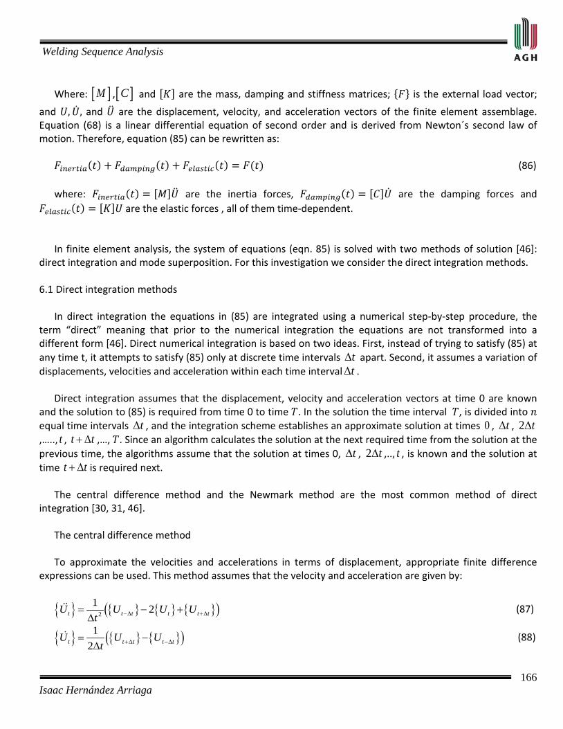
Welding Sequence Analysis
166 Isaac Hernández Arriaga
Where: [ ]M ,[ ]C and are the mass, damping and stiffness matrices; is the external load vector;
and and are the displacement, velocity, and acceleration vectors of the finite element assemblage. Equation (68) is a linear differential equation of second order and is derived from Newton´s second law of motion. Therefore, equation (85) can be rewritten as: (86) where: are the inertia forces, are the damping forces and
are the elastic forces , all of them time-dependent. In finite element analysis, the system of equations (eqn. 85) is solved with two methods of solution [46]: direct integration and mode superposition. For this investigation we consider the direct integration methods. 6.1 Direct integration methods In direct integration the equations in (85) are integrated using a numerical step-by-step procedure, the term “direct” meaning that prior to the numerical integration the equations are not transformed into a different form [46]. Direct numerical integration is based on two ideas. First, instead of trying to satisfy (85) at any time t, it attempts to satisfy (85) only at discrete time intervals t∆ apart. Second, it assumes a variation of displacements, velocities and acceleration within each time interval t∆ . Direct integration assumes that the displacement, velocity and acceleration vectors at time 0 are known and the solution to (85) is required from time 0 to time . In the solution the time interval , is divided into equal time intervals t∆ , and the integration scheme establishes an approximate solution at times 0 , t∆ , 2 t∆,….., t , t t+ ∆ ,…, . Since an algorithm calculates the solution at the next required time from the solution at the previous time, the algorithms assume that the solution at times 0, t∆ , 2 t∆ ,.., t , is known and the solution at time t t+ ∆ is required next. The central difference method and the Newmark method are the most common method of direct integration [30, 31, 46]. The central difference method To approximate the velocities and accelerations in terms of displacement, appropriate finite difference expressions can be used. This method assumes that the velocity and acceleration are given by:
{ } { } { } { }( )2
1 2t t t t t tU U U Ut −∆ +∆= − +
∆ (87)
{ } { } { }( )12t t t t tU U U
t +∆ −∆= −∆
(88)
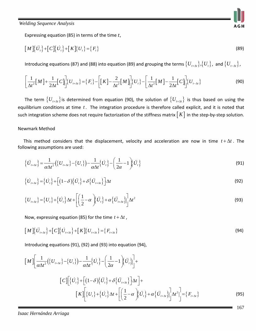
Welding Sequence Analysis
167 Isaac Hernández Arriaga
Expressing equation (85) in terms of the time , [ ]{ } [ ]{ } [ ]{ } { }t t t tM U C U K U F+ + = (89)
Introducing equations (87) and (88) into equation (89) and grouping the terms { } { },t t tU U+∆ , and { }t tU −∆ ,
[ ] [ ] { } { } [ ] [ ] { } [ ] [ ] { }2 2 2
1 1 2 1 12 2t t t t t tM C U F K M U M C U
t t t t t+∆ −∆ + = − − − − ∆ ∆ ∆ ∆ ∆
(90)
The term { }t tU +∆ is determined from equation (90), the solution of { }t tU +∆ is thus based on using the
equilibrium conditions at time t . The integration procedure is therefore called explicit, and it is noted that
such integration scheme does not require factorization of the stiffness matrix [ ]K in the step-by-step solution.
Newmark Method This method considers that the displacement, velocity and acceleration are now in time t t+ ∆ . The following assumptions are used:
{ } { } { }( ) { } { }2
1 1 1 12t t t t t t tU U U U U
t tα α α+∆ +∆ = − − − − ∆ ∆
(91)
{ } { } ( ){ } { }1t t t t t tU U U U tδ δ+∆ +∆ = + − + ∆
(92)
{ } { } { } { } { } 212t t t t t t tU U U t U U tα α+∆ +∆
= + ∆ + − + ∆ (93)
Now, expressing equation (85) for the time t t+ ∆ , [ ]{ } [ ]{ } [ ]{ } { }t t t t t t t tM U C U K U F+∆ +∆ +∆ +∆+ + = (94)
Introducing equations (91), (92) and (93) into equation (94),
[ ] { } { }( ) { } { }2
1 1 1 12t t t t tM U U U U
t tα α α+∆
− − − − + ∆ ∆
[ ] { } ( ){ } { }1t t t tC U U U tδ δ +∆ + − + ∆ +
[ ] { } { } { } { } { }212t t t t t t tK U U t U U t Fα α +∆ +∆
+ ∆ + − + ∆ = (95)
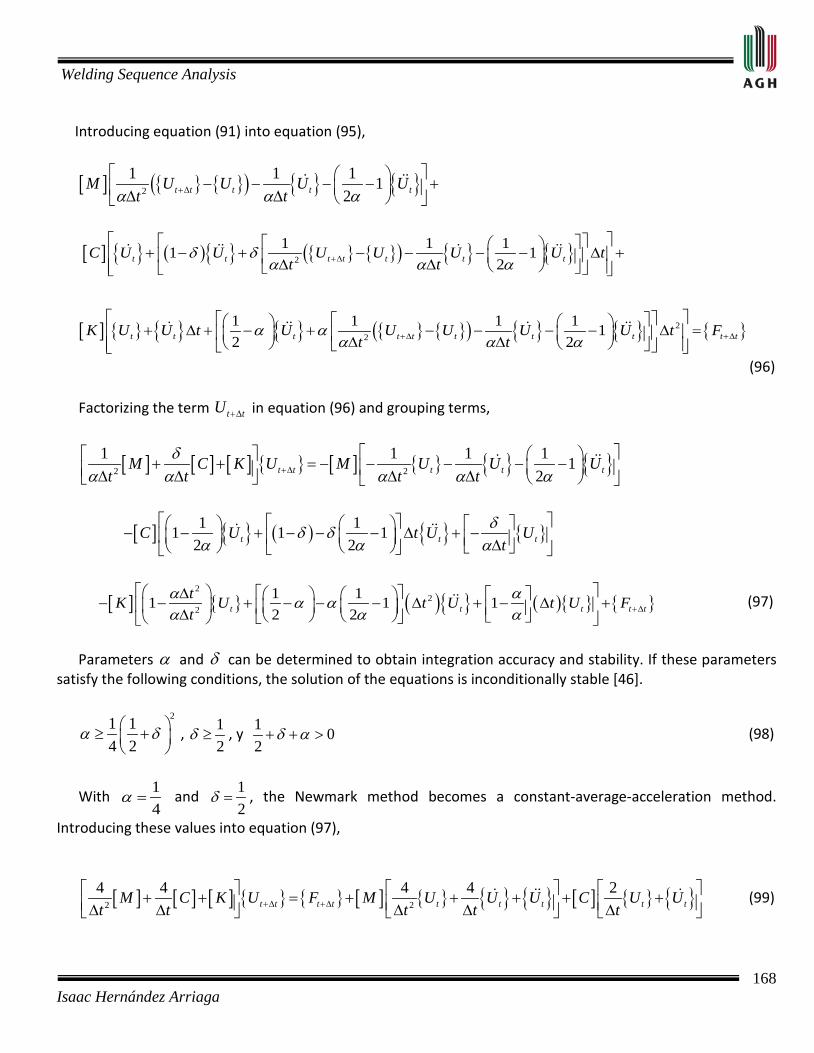
Welding Sequence Analysis
168 Isaac Hernández Arriaga
Introducing equation (91) into equation (95),
[ ] { } { }( ) { } { }2
1 1 1 12t t t t tM U U U U
t tα α α+∆
− − − − + ∆ ∆
[ ] { } ( ){ } { } { }( ) { } { }2
1 1 11 12t t t t t t tC U U U U U U t
t tδ δ
α α α+∆
+ − + − − − − ∆ + ∆ ∆
[ ] { } { } { } { } { }( ) { } { } { }2
2
1 1 1 1 12 2t t t t t t t t t tK U U t U U U U U t F
t tα α
α α α+∆ +∆
+ ∆ + − + − − − − ∆ = ∆ ∆
(96) Factorizing the term t tU +∆ in equation (96) and grouping terms,
[ ] [ ] [ ] { } [ ] { } { } { }2 2
1 1 1 1 12t t t t tM C K U M U U U
t t t tδ
α α α α α+∆
+ + = − − − − − ∆ ∆ ∆ ∆
[ ] { } ( ) { } { }1 11 1 12 2t t tC U t U U
tδδ δ
α α α − − + − − − ∆ + − ∆
[ ] { } ( ){ } ( ){ } { }2
22
1 11 1 12 2t t t t t
tK U t U t U Ft
α αα αα α α +∆
∆ − − + − − − ∆ + − ∆ + ∆ (97)
Parameters α and δ can be determined to obtain integration accuracy and stability. If these parameters satisfy the following conditions, the solution of the equations is inconditionally stable [46].
21 1
4 2α δ ≥ +
,
12
δ ≥ , y 1 02
δ α+ + > (98)
With 14
α = and 12
δ = , the Newmark method becomes a constant-average-acceleration method.
Introducing these values into equation (97),
[ ] [ ] [ ] { } { } [ ] { } { } { } [ ] { } { }2 2
4 4 4 4 2t t t t t t t t tM C K U F M U U U C U U
t t t t t+∆ +∆ + + = + + + + + ∆ ∆ ∆ ∆ ∆
(99)
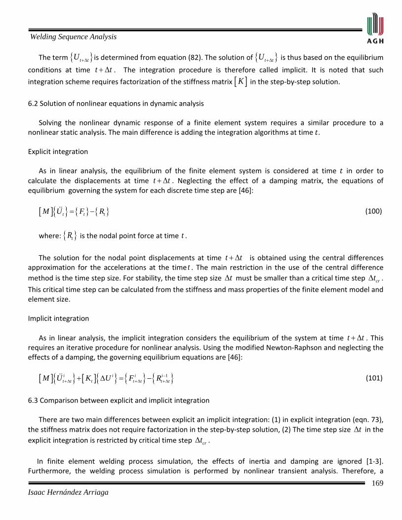
Welding Sequence Analysis
169 Isaac Hernández Arriaga
The term { }t tU +∆ is determined from equation (82). The solution of { }t tU +∆ is thus based on the equilibrium
conditions at time t t+ ∆ . The integration procedure is therefore called implicit. It is noted that such
integration scheme requires factorization of the stiffness matrix [ ]K in the step-by-step solution.
6.2 Solution of nonlinear equations in dynamic analysis Solving the nonlinear dynamic response of a finite element system requires a similar procedure to a nonlinear static analysis. The main difference is adding the integration algorithms at time . Explicit integration As in linear analysis, the equilibrium of the finite element system is considered at time in order to calculate the displacements at time t t+ ∆ . Neglecting the effect of a damping matrix, the equations of equilibrium governing the system for each discrete time step are [46]: [ ]{ } { } { }t t tM U F R= − (100)
where: { }tR is the nodal point force at time t .
The solution for the nodal point displacements at time t t+ ∆ is obtained using the central differences approximation for the accelerations at the time t . The main restriction in the use of the central difference method is the time step size. For stability, the time step size t∆ must be smaller than a critical time step crt∆ .
This critical time step can be calculated from the stiffness and mass properties of the finite element model and element size. Implicit integration As in linear analysis, the implicit integration considers the equilibrium of the system at time t t+ ∆ . This requires an iterative procedure for nonlinear analysis. Using the modified Newton-Raphson and neglecting the effects of a damping, the governing equilibrium equations are [46]: [ ]{ } [ ]{ } { } { }1i i i i
t t t t t t tM U K U F R −+∆ +∆ +∆+ ∆ = − (101)
6.3 Comparison between explicit and implicit integration There are two main differences between explicit an implicit integration: (1) in explicit integration (eqn. 73), the stiffness matrix does not require factorization in the step-by-step solution, (2) The time step size t∆ in the explicit integration is restricted by critical time step crt∆ .
In finite element welding process simulation, the effects of inertia and damping are ignored [1-3]. Furthermore, the welding process simulation is performed by nonlinear transient analysis. Therefore, a
Welding Sequence Analysis
170 Isaac Hernández Arriaga
commercial finite element code with explicit integration is not appropriate because the time step size limitation may considerably slow down calculations. Also, equation (83), which is obtained by finite element method for a thermal elastic plastic model has the form of the implicit integration equation (eqn. 101) neglect the effects of inertia and damping. Therefore, a commercial package that uses the implicit integration is more appropriate for the simulation of the welding process.

Welding Sequence Analysis
171 Isaac Hernández Arriaga
APPENDIX 2

Welding Sequence Analysis
172 Isaac Hernández Arriaga
Definition and justification of the applied finite elements The proposed sequentially-coupled thermo-mechanical analysis involves two steps. In the first step a transient heat transfer analysis is performed followed by a thermal elastic plastic analysis. To perform the thermal analysis, it is necessary to select an element type that can simulate:
• Transient thermal analysis.
• The weld thermal cycle [figure 3.6, page 58], which determines the temperature as a function of time in the weld bead (i.e., all elements belonging to the weld bead).
• Conduction heat transfer in the base metal.
• Heat loss by convection and radiation to the surroundings in the base metal.
• Activation and de-activation of the weld bead elements. To perform the structural analysis, it is necessary to select an element type that can simulate:
• Homogeneous and isotropic material.
• Elastic-plastic material behavior following the von Mises yield criterion and the associated flow rule with linear isotropic hardening by strain.
• Small strains.
• Activation and de-activation of the weld bead elements. An important factor for the selection of the structural element is the stress state for each analyzed structure, as determined below (figures 7 to 10). The analysis reveals that all structures develop bending stiffness effects, except for the I-type structure subject to tension. ANSYS offers a broad variety of elements for the analysis of two and three-dimensional thermal and structural problems such as BEAM, SHELL, PLANE and SOLID elements. All these elements can simulate mechanical and thermal effects in addition to bending stiffness. The plane and solid elements solved this bending condition with the link between several elements. Beam elements are appropriate for structural members whose cross-sectional dimensions are small compared to its length. They are also commonly subjected to transverse loading. Shell elements are designed to efficiently model thin structures and bending capability. Otherwise, these elements present initial instability in perfectly flat plates. Avoiding this effect requires an initial displacement. Beam and shell elements are therefore discarded while the plane and solid elements are selected for the numerical simulation. 1.- I-type structure subject to tension. This structure consists of a central bar and two lateral bars (three parallel bars joined together). Due to the symmetry of the structure, only a quarter of the model is analyzed as is shown in figure 7(a). The stress state is
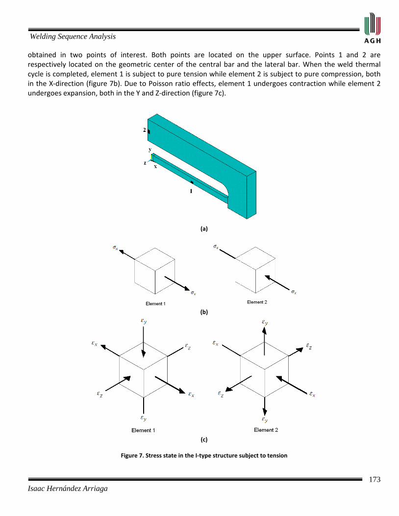
Welding Sequence Analysis
173 Isaac Hernández Arriaga
obtained in two points of interest. Both points are located on the upper surface. Points 1 and 2 are respectively located on the geometric center of the central bar and the lateral bar. When the weld thermal cycle is completed, element 1 is subject to pure tension while element 2 is subject to pure compression, both in the X-direction (figure 7b). Due to Poisson ratio effects, element 1 undergoes contraction while element 2 undergoes expansion, both in the Y and Z-direction (figure 7c).
(a)
(b)
(c)
Figure 7. Stress state in the I-type structure subject to tension
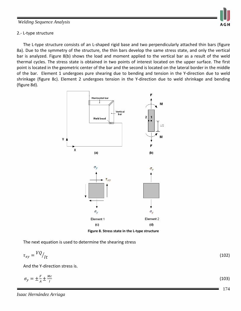
Welding Sequence Analysis
174 Isaac Hernández Arriaga
2.- L-type structure The L-type structure consists of an L-shaped rigid base and two perpendicularly attached thin bars (figure 8a). Due to the symmetry of the structure, the thin bars develop the same stress state, and only the vertical bar is analyzed. Figure 8(b) shows the load and moment applied to the vertical bar as a result of the weld thermal cycles. The stress state is obtained in two points of interest located on the upper surface. The first point is located in the geometric center of the bar and the second is located on the lateral border in the middle of the bar. Element 1 undergoes pure shearing due to bending and tension in the Y-direction due to weld shrinkage (figure 8c). Element 2 undergoes tension in the Y-direction due to weld shrinkage and bending (figure 8d).
Figure 8. Stress state in the L-type structure
The next equation is used to determine the shearing stress
(102)
And the Y-direction stress is.
(103)

Welding Sequence Analysis
175 Isaac Hernández Arriaga
3.- Stiffened symmetrical flat frame (flat stress condition) Stiffened symmetrical flat frame consists of four external bars and three internal bars joined by ten welds (figure 9a). Figure 9(b) shows the load and moment applied to one half of the external vertical bar as a result of the weld thermal cycles. The stress state is obtained in two points of interest. Both points are located on the upper surface. The first is located in the geometric center of the extracted segment from the external vertical bar and the second is located on the lateral border in the middle of the extracted segment. Element 1 undergoes pure shearing due to bending and tension in the Y-direction due to the weld shrinkage (figure 9c). Element 2 undergoes tension in the Y-direction due to weld shrinkage and bending (figure 9d). The shearing stress ( ) and stress ( ) are respectively determined by equations (120) and (103).
Figure 9. Stress state in the stiffened symmetrical flat frame

Welding Sequence Analysis
176 Isaac Hernández Arriaga
4.- 3-Dimensional unitary cell - type symmetrical structure The 3-dimensional unitary cell consists of two horizontal and two vertical plates joined by fillet welds (figure 10a). Figure 10(b) shows the moments applied to a segment of the vertical plate as a result of the weld thermal cycles. This segment is delimited in the Y-direction by the weld beads and in the Z-direction by the plate´s lateral borders. The stress state is obtained in one point of interest located on the upper surface in the geometric center of the segment from the vertical plate. Element 1 undergoes shearing and tension in the Y and Z-direction due to bending and to the weld shrinkage (figure 10c). The shearing stress ( ) and stress ( ) are respectively determined by equations (120) and (103).
Figure 10. Stress state in the 3-Dimensional unitary cell Tables 1 and 2 show some plane and solid elements commonly used by ANSYS. In general, all elements have the same characteristics (degree of freedom, input data, and output data), except for two main differences: 1) the order of elements: higher order elements achieve better results and greater accuracy, however, these elements require more computational time because numerical integration of elemental matrices is more involved. Higher order elements are well suited to problems with curved boundaries. 2) The

Welding Sequence Analysis
177 Isaac Hernández Arriaga
shape of element: quadrilateral and brick element present better meshing control than triangular and tetrahedral elements.
For these two reasons, PLANE55 and SOLID70 elements are respectively selected for two and three dimensional thermal analysis. Both elements have isotropic material properties and a single degree of freedom: temperature. These elements allow straightforward thermal modeling of the welding process, including thermal conductivity and specific heat as a function of temperature (Fig 3.3, page 56). The convective heat transfer coefficient is considered constant at 10 W/m2
THERMAL ELEMENTS
ºC (natural convection). Heat loss by convection is a boundary condition and is applied only to surfaces in contact with the surrounding air – assumed at 20°C, same as the initial temperature of the base metal. The elements PLANE42 and SOLID45 are respectively selected for two and three dimensional structural analysis. PLANE 42 and SOLID45 elements have isotropic material properties and respectively two and three degrees of freedom at each node: translation in the nodal directions. Both elements couple temperatures with strain, therefore requiring the thermal expansion coefficient, elasticity modulus, tangent modulus, yield stress and Poisson´s ratio dependent on temperature (figure 3.3 page 56). Finally, thermal loads are transferred to the structural analysis through the concept of body load used through load step. PLANE 42 and SOLID45 elements have this capability because the temperatures may be specified as body loads at the nodes. The elements PLANE42 and SOLID55, and SOLID70 and SOLID45 are equivalent to performing coupled thermo-mechanical analysis.
Element Dimension Number of nodes
Main application
Degree of freedom
Input data Output data Comments
PLANE35 2-D triangular element
6 Steady-state and transient conduction Heat transfer
Temperature - Convection or heat fluxes may be applied to the element´s surfaces.
- Nodal temperatures. - Thermal gradients. - Thermal fluxes components.
-This element is compatible with the PLANE77 element.
PLANE55 2-D quadrilateral element
4 Steady-state and transient conduction Heat transfer
Temperature - Convection or heat fluxes may be applied to the element´s surfaces.
- Nodal temperatures. - Thermal gradients. - Thermal fluxes components.
- Better meshing control
PLANE77 2-D quadrilateral element
8 Steady-state and transient conduction Heat transfer
Temperature - Convection or heat fluxes may be applied to the element´s surfaces.
- Nodal temperatures. - Thermal gradients. - Thermal fluxes components.
- This element is well suited to model problems with curved boundaries.
SOLID70 3-D brick element
8 Steady-state and transient conduction Heat transfer
Temperature - Convection or heat fluxes may be applied to the element´s surfaces. -Heat generation rates may be applied at the nodes.
- Nodal temperatures. - Average face temperature. - Temperature-gradient components. - Vector sum at the centroid of the element. - Heat flux components.
- Better meshing control
SOLID90 3-D brick element
20 Steady-state and transient conduction Heat transfer
Temperature - Convection or heat fluxes may be applied to the element´s surfaces. -Heat generation rates may be applied at the nodes.
- Nodal temperatures. - Average face temperature. - Temperature-gradient components. - Vector sum at the centroid of the element. - Heat flux components.
- This element is well suited to model problems with curved boundaries.
Table 1. Thermal (conduction) elements used by ANSYS

Welding Sequence Analysis
178 Isaac Hernández Arriaga
STRUCTURAL ELEMENTS
Element Dimension Number of nodes
Main application
Degree of freedom
Input data Output data Comments
PLANE42 2-D quadrilateral
element
4 Isotropic solid problems
Translation in the nodal x and y-directions
-Distributed surface load may be applied to element´s surfaces. -Temperatures may be input as element body loads at the nodes.
- Nodal displacements. - Directional stress and principal stresses.
- Better meshing control. -This element may be used to analyze large-deflection, large-strain, plasticity, and creep problems
PLANE82 2-D quadrilateral
element
8 Isotropic solid problems
Translation in the nodal x and y-directions
-Distributed surface load may be applied to element´s surfaces. -Temperatures may be input as element body loads at the nodes.
- Nodal displacements. - Directional stress and principal stresses.
- This element is well suited to model problems with curved boundaries. -This element may be used to analyze large-deflection, large-strain, plasticity, and creep problems
SOLID45 3-D brick element
8 Isotropic solid problems
Translation in the nodal x, y, and z- directions
- Distributed surface load may be applied to element´s surfaces. -Temperatures may be input as element body loads at the nodes.
- Nodal displacements. - Normal components of the stress in x, y, and z-directions; shear stress and principal stresses.
-This element may be used to analyze large-deflection, large-strain, plasticity, and creep problems
SOLID92 3-D tetrahedral
element
10 Isotropic solid problems
Translation in the nodal x, y, and z- directions
- Distributed surface load may be applied to element´s surfaces. -Temperatures may be input as element body loads at the nodes.
- Nodal displacements. - Normal components of the stress in x, y, and z-directions; shear stress and principal stresses.
-This element may be used to analyze large-deflection, large-strain, plasticity, and creep problems
Table 2. Structural elements used by ANSYS
Welding Sequence Analysis
179 Isaac Hernández Arriaga
APPENDIX 3
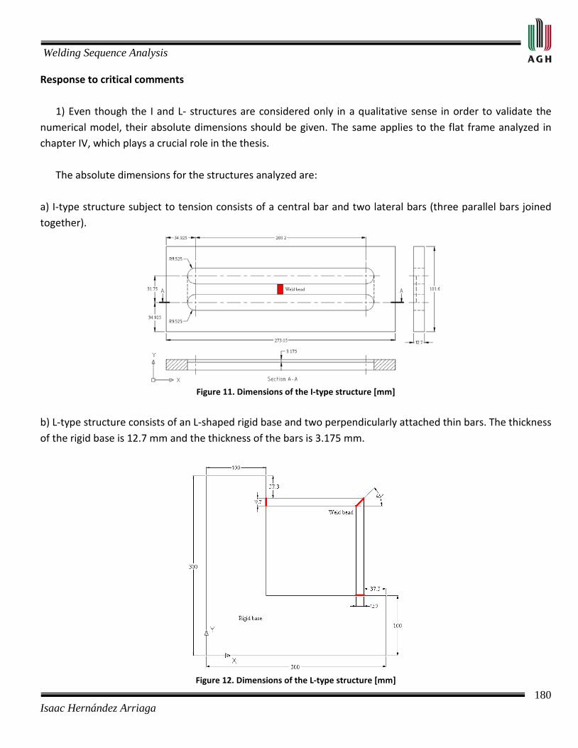
Welding Sequence Analysis
180 Isaac Hernández Arriaga
Response to critical comments 1) Even though the I and L- structures are considered only in a qualitative sense in order to validate the numerical model, their absolute dimensions should be given. The same applies to the flat frame analyzed in chapter IV, which plays a crucial role in the thesis. The absolute dimensions for the structures analyzed are: a) I-type structure subject to tension consists of a central bar and two lateral bars (three parallel bars joined together).
Figure 11. Dimensions of the I-type structure [mm]
b) L-type structure consists of an L-shaped rigid base and two perpendicularly attached thin bars. The thickness of the rigid base is 12.7 mm and the thickness of the bars is 3.175 mm.
Figure 12. Dimensions of the L-type structure [mm]
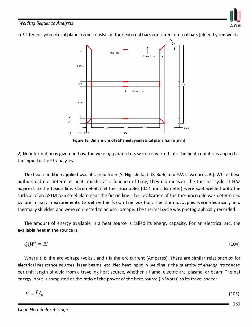
Welding Sequence Analysis
181 Isaac Hernández Arriaga
c) Stiffened symmetrical plane frame consists of four external bars and three internal bars joined by ten welds.
Figure 13. Dimensions of stiffened symmetrical plane frame [mm]
2) No information is given on how the welding parameters were converted into the heat conditions applied as the input to the FE analyses. The heat condition applied was obtained from [Y. Higashida, J. D. Burk, and F.V. Lawrence, JR.]. While these authors did not determine heat transfer as a function of time, they did measure the thermal cycle at HAZ adjacent to the fusion line. Chromel-alumel thermocouples (0.51 mm diameter) were spot welded onto the surface of an ASTM A36 steel plate near the fusion line. The localization of the thermocouple was determined by preliminary measurements to define the fusion line position. The thermocouples were electrically and thermally shielded and were connected to an oscilloscope. The thermal cycle was photographically recorded. The amount of energy available in a heat source is called its energy capacity. For an electrical arc, the available heat at the source is: (104) Where E is the arc voltage (volts), and I is the arc current (Amperes). There are similar relationships for electrical resistance sources, laser beams, etc. Net heat input in welding is the quantity of energy introduced per unit length of weld from a traveling heat source, whether a flame, electric arc, plasma, or beam. The net energy input is computed as the ratio of the power of the heat source (in Watts) to its travel speed:
(105)
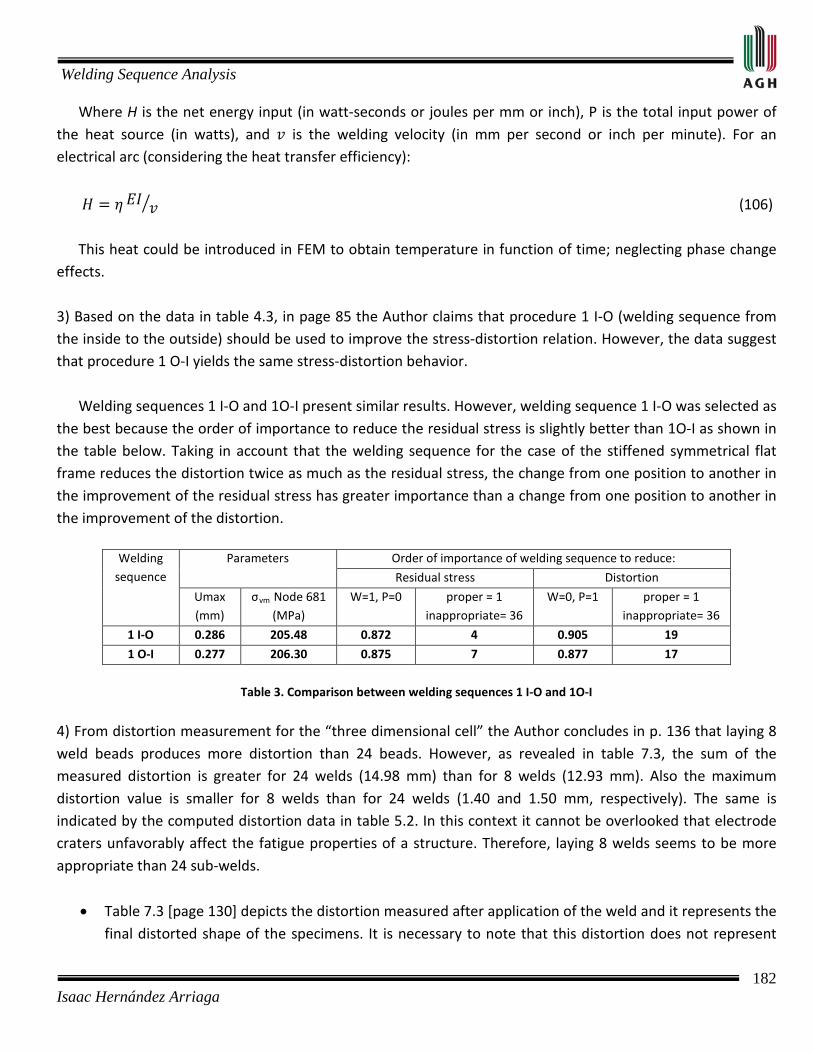
Welding Sequence Analysis
182 Isaac Hernández Arriaga
Where H is the net energy input (in watt-seconds or joules per mm or inch), P is the total input power of the heat source (in watts), and is the welding velocity (in mm per second or inch per minute). For an electrical arc (considering the heat transfer efficiency):
(106) This heat could be introduced in FEM to obtain temperature in function of time; neglecting phase change effects. 3) Based on the data in table 4.3, in page 85 the Author claims that procedure 1 I-O (welding sequence from the inside to the outside) should be used to improve the stress-distortion relation. However, the data suggest that procedure 1 O-I yields the same stress-distortion behavior. Welding sequences 1 I-O and 1O-I present similar results. However, welding sequence 1 I-O was selected as the best because the order of importance to reduce the residual stress is slightly better than 1O-I as shown in the table below. Taking in account that the welding sequence for the case of the stiffened symmetrical flat frame reduces the distortion twice as much as the residual stress, the change from one position to another in the improvement of the residual stress has greater importance than a change from one position to another in the improvement of the distortion.
Welding sequence
Parameters Order of importance of welding sequence to reduce:
Residual stress Distortion
Umax (mm)
σvm W=1, P=0 Node 681 (MPa)
proper = 1 inappropriate= 36
W=0, P=1 proper = 1 inappropriate= 36
1 I-O 0.286 205.48 0.872 4 0.905 19
1 O-I 0.277 206.30 0.875 7 0.877 17
Table 3. Comparison between welding sequences 1 I-O and 1O-I
4) From distortion measurement for the “three dimensional cell” the Author concludes in p. 136 that laying 8 weld beads produces more distortion than 24 beads. However, as revealed in table 7.3, the sum of the measured distortion is greater for 24 welds (14.98 mm) than for 8 welds (12.93 mm). Also the maximum distortion value is smaller for 8 welds than for 24 welds (1.40 and 1.50 mm, respectively). The same is indicated by the computed distortion data in table 5.2. In this context it cannot be overlooked that electrode craters unfavorably affect the fatigue properties of a structure. Therefore, laying 8 welds seems to be more appropriate than 24 sub-welds.
• Table 7.3 [page 130] depicts the distortion measured after application of the weld and it represents the final distorted shape of the specimens. It is necessary to note that this distortion does not represent
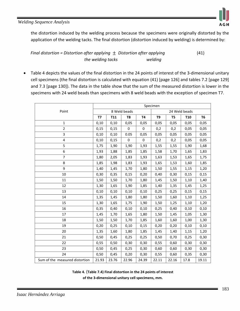
Welding Sequence Analysis
183 Isaac Hernández Arriaga
the distortion induced by the welding process because the specimens were originally distorted by the application of the welding tacks. The final distortion (distortion induced by welding) is determined by:
Final distortion = Distortion after applying Distortion after applying (41)
the welding tacks welding
• Table 4 depicts the values of the final distortion in the 24 points of interest of the 3-dimensional unitary cell specimens (the final distortion is calculated with equation (41) [page 126] and tables 7.2 [page 129] and 7.3 [page 130]). The data in the table show that the sum of the measured distortion is lower in the specimens with 24 weld beads than specimens with 8 weld beads with the exception of specimen T7.
Point
Specimen
8 Weld beads 24 Weld beads
T7 T11 T8 T4 T9 T5 T10 T6
1 0,10 0,10 0,05 0,05 0,05 0,05 0,05 0,05
2 0,15 0,15 0 0 0,2 0,2 0,05 0,05
3 0,10 0,10 0.05 0,05 0,05 0,05 0,05 0,05
4 0,10 0,15 0 0 0,2 0,2 0,05 0,05
5 1,75 1,90 1,90 1,93 1,55 1,55 1,90 1,68
6 1,93 1,88 1,85 1,85 1,58 1,70 1,65 1,83
7 1,80 2,05 1,83 1,93 1,63 1,53 1,65 1,75
8 1,85 1,98 1,83 1,93 1,65 1,53 1,60 1,85
9 1,40 1,45 1,70 1,80 1,50 1,55 1,15 1,20
10 0,30 0,35 0,15 0,20 0,40 0,30 0,15 0,15
11 1,50 1,50 1,70 1,80 1,45 1,50 1,10 1,40
12 1,30 1,65 1,90 1,85 1,40 1,35 1,45 1,25
13 0,10 0,10 0,10 0,10 0,25 0,25 0,15 0,15
14 1,35 1,45 1,80 1,80 1,50 1,60 1,10 1,25
15 1,30 1,65 1,75 1,90 1,50 1,25 1,10 1,20
16 0,35 0,40 0,10 0,10 0,25 0,40 0,10 0,10
17 1,45 1,70 1,65 1,80 1,50 1,45 1,05 1,30
18 1,50 1,50 1,70 1,85 1,60 1,60 1,00 1,30
19 0,20 0,25 0,10 0,15 0,20 0,20 0,10 0,10
20 1,35 1,60 1,80 1,85 1,45 1,40 1,15 1,20
21 0,50 0,45 0,25 0,25 0,50 0,70 0,25 0,30
22 0,55 0,50 0,30 0,30 0,55 0,60 0,30 0,30
23 0,50 0,45 0,25 0,30 0,60 0,60 0,30 0,30
24 0,50 0,45 0,20 0,30 0,55 0,60 0,35 0,30
Sum of the measured distortion 21.93 23.76 22.96 24.39 22.11 22.16 17.8 19.11
Table 4. (Table 7.4) Final distortion in the 24 points of interest of the 3-dimensional unitary cell specimens, mm.

Welding Sequence Analysis
184 Isaac Hernández Arriaga
• Table 5 depicts the computed distortion at the 24 points of interest for the different welding sequences. The table shows that simulations 3 and 4 (with 24 weld beads) produce lower distortion than the others (with 8 weld beads).
Point Node Simulation
8 weld beads 24 weld beads
1 2 3 4
1 15756 0,08 0,05 0,06 0,04
2 17536 0,11 0,01 0,21 0,05
3 19015 0,08 0,07 0,06 0,04
4 17238 0,11 0,02 0,21 0,05
5 14571 1,85 1,87 1,68 1,65
6 20554 2,0 2,0 1,75 1,85
7 20508 1,82 1,83 1,67 1,64
8 14498 1,99 1,98 1,73 1,80
9 11 1,36 1,70 1,52 1,12
10 386 0,31 0,18 0,35 0,19
11 758 1,54 1,92 1,53 1,13
12 35172 1,49 1,86 1,55 1,11
13 38137 0,08 0,07 0,2 0,19
14 41155 1,57 1,95 1,74 1,24
15 35099 1,51 1,88 1,50 1,08
16 37839 0,39 0,10 0,3 0,08
17 41109 1,33 1,65 1,54 1,13
18 1 1,56 1,94 1,74 1,21
19 361 0,19 0,10 0,16 0,08
20 754 1,47 1,83 1,56 1,01
21 167 0,57 0,25 0,66 0,29
22 36357 0,59 0,34 0,59 0,34
23 591 0,57 0,31 0,6 0,33
24 39616 0,52 0,22 0,68 0,29
Maximum distortion
2,97 3,05 2,04 2,10
Table 5. (Table 5.2) Distortion at the 24 points of interest corresponding to different welding sequences
In the 3-dimensional unitary cell structure, mm.
• Structures with a greater number of sub-welds are more appropriate to reduce distortion, but also reduce fatigue performance due to higher residual stresses which may reach the yield point in normal operating conditions. Therefore, to avoid the loss of stability, laying 8 weld beads seems to be more appropriate than 24 sub-welds.
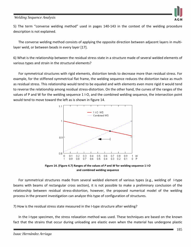
Welding Sequence Analysis
185 Isaac Hernández Arriaga
5) The term “converse welding method” used in pages 140-143 in the context of the welding procedure description is not explained. The converse welding method consists of applying the opposite direction between adjacent layers in multi-layer weld, or between beads in every layer [17]. 6) What is the relationship between the residual stress state in a structure made of several welded elements of various types and strain in the structural elements? For symmetrical structures with rigid elements, distortion tends to decrease more than residual stress. For example, for the stiffened symmetrical flat frame, the welding sequence reduces the distortion twice as much as residual stress. This relationship would tend to be equaled and with elements even more rigid it would tend to reverse the relationship among residual stress-distortion. On the other hand, the curves of the ranges of the values of P and W for the welding sequence 1 I-O, and the combined welding sequence, the intersection point would tend to move toward the left as is shown in figure 14.
Figure 14. (Figure 4.7) Ranges of the values of P and W for welding sequence 1 I-O
and combined welding sequence
For symmetrical structures made from several welded element of various types (e.g., welding of I-type beams with beams of rectangular cross section), it is not possible to make a preliminary conclusion of the relationship between residual stress-distortion, however, the proposed numerical model of the welding process in the present investigation can analyze this type of configuration of structures. 7) How is the residual stress state measured in the I-type structure after welding? In the I-type specimen, the stress relaxation method was used. These techniques are based on the known fact that the strains that occur during unloading are elastic even when the material has undergone plastic
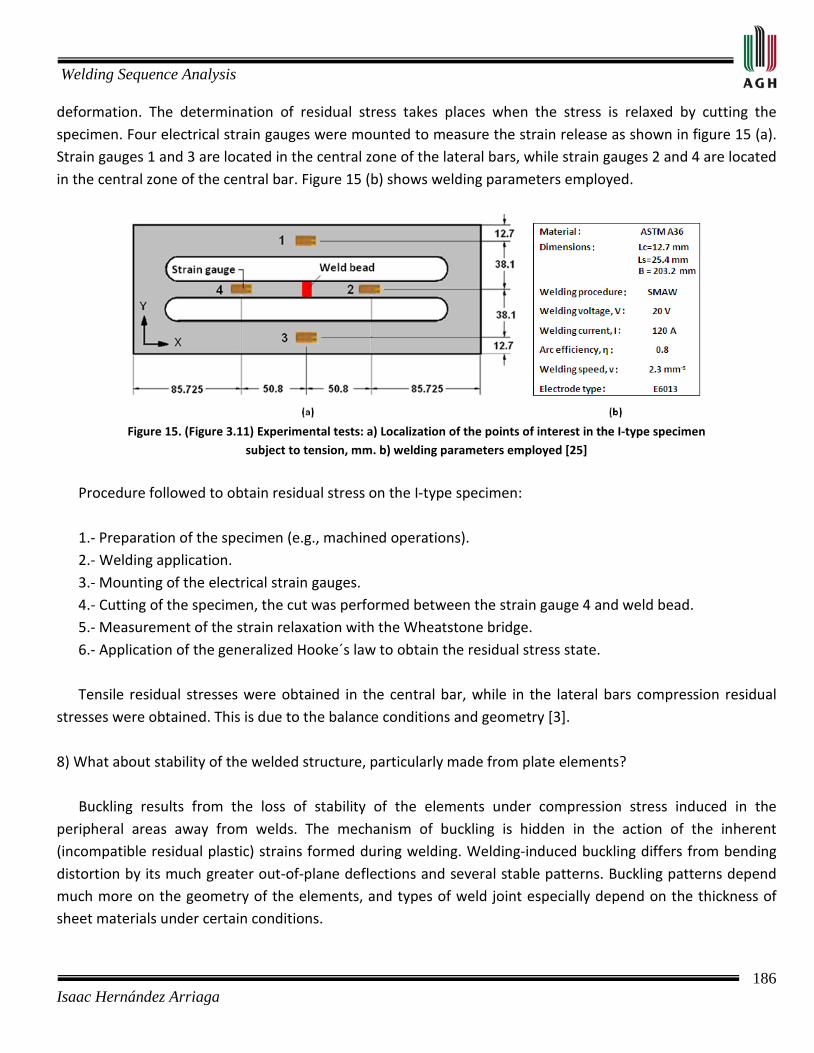
Welding Sequence Analysis
186 Isaac Hernández Arriaga
deformation. The determination of residual stress takes places when the stress is relaxed by cutting the specimen. Four electrical strain gauges were mounted to measure the strain release as shown in figure 15 (a). Strain gauges 1 and 3 are located in the central zone of the lateral bars, while strain gauges 2 and 4 are located in the central zone of the central bar. Figure 15 (b) shows welding parameters employed.
Figure 15. (Figure 3.11) Experimental tests: a) Localization of the points of interest in the I-type specimen
subject to tension, mm. b) welding parameters employed [25]
Procedure followed to obtain residual stress on the I-type specimen: 1.- Preparation of the specimen (e.g., machined operations). 2.- Welding application. 3.- Mounting of the electrical strain gauges. 4.- Cutting of the specimen, the cut was performed between the strain gauge 4 and weld bead. 5.- Measurement of the strain relaxation with the Wheatstone bridge. 6.- Application of the generalized Hooke´s law to obtain the residual stress state. Tensile residual stresses were obtained in the central bar, while in the lateral bars compression residual stresses were obtained. This is due to the balance conditions and geometry [3]. 8) What about stability of the welded structure, particularly made from plate elements? Buckling results from the loss of stability of the elements under compression stress induced in the peripheral areas away from welds. The mechanism of buckling is hidden in the action of the inherent (incompatible residual plastic) strains formed during welding. Welding-induced buckling differs from bending distortion by its much greater out-of-plane deflections and several stable patterns. Buckling patterns depend much more on the geometry of the elements, and types of weld joint especially depend on the thickness of sheet materials under certain conditions.
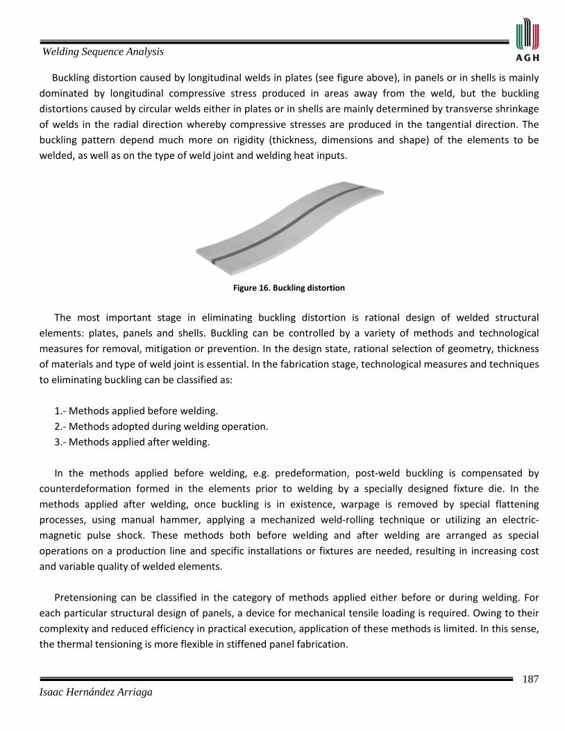
Welding Sequence Analysis
187 Isaac Hernández Arriaga
Buckling distortion caused by longitudinal welds in plates (see figure above), in panels or in shells is mainly dominated by longitudinal compressive stress produced in areas away from the weld, but the buckling distortions caused by circular welds either in plates or in shells are mainly determined by transverse shrinkage of welds in the radial direction whereby compressive stresses are produced in the tangential direction. The buckling pattern depend much more on rigidity (thickness, dimensions and shape) of the elements to be welded, as well as on the type of weld joint and welding heat inputs.
Figure 16. Buckling distortion
The most important stage in eliminating buckling distortion is rational design of welded structural elements: plates, panels and shells. Buckling can be controlled by a variety of methods and technological measures for removal, mitigation or prevention. In the design state, rational selection of geometry, thickness of materials and type of weld joint is essential. In the fabrication stage, technological measures and techniques to eliminating buckling can be classified as: 1.- Methods applied before welding. 2.- Methods adopted during welding operation. 3.- Methods applied after welding. In the methods applied before welding, e.g. predeformation, post-weld buckling is compensated by counterdeformation formed in the elements prior to welding by a specially designed fixture die. In the methods applied after welding, once buckling is in existence, warpage is removed by special flattening processes, using manual hammer, applying a mechanized weld-rolling technique or utilizing an electric-magnetic pulse shock. These methods both before welding and after welding are arranged as special operations on a production line and specific installations or fixtures are needed, resulting in increasing cost and variable quality of welded elements. Pretensioning can be classified in the category of methods applied either before or during welding. For each particular structural design of panels, a device for mechanical tensile loading is required. Owing to their complexity and reduced efficiency in practical execution, application of these methods is limited. In this sense, the thermal tensioning is more flexible in stiffened panel fabrication.

Welding Sequence Analysis
188 Isaac Hernández Arriaga
APPENDIX 4

Welding Sequence Analysis
189 Isaac Hernández Arriaga
Proper welding sequence to reduce residual stress and distortion in common symmetrical structures in 2 and 3 dimensions based on the hypothesis developed in the sections 4.9 and 5.2. Welding of the collinear tubes with 8 weld beads
Collinear tubes Welding Proper welding sequence to reduce residual stress and/or distortion
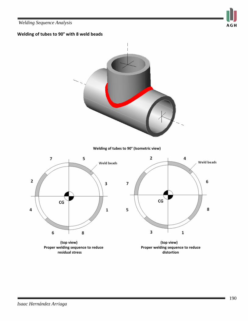
Welding Sequence Analysis
190 Isaac Hernández Arriaga
Welding of tubes to 90° with 8 weld beads
Welding of tubes to 90° (Isometric view)
(top view) (top view) Proper welding sequence to reduce Proper welding sequence to reduce residual stress distortion

Welding Sequence Analysis
191 Isaac Hernández Arriaga
APPENDIX 5
Welding Sequence Analysis
192 Isaac Hernández Arriaga
Listing of commands of the numerical simulation of the welding process (I-type specimen subject to tension) Transient thermal analysis /title,transient thermal analysis /PREP7 k,1,0,0 k,2,0.0015,0 k,3,0.003,0 k,4,0.00635,0 k,5,0.0127,0 k,6,0.0254,0 k,7,0.0381,0 k,8,0.0508,0 k,9,0.06985,0 k,10,0.101575,0 k,11,0.1100840,0 k,12,0.1365,0 k,13,0,0.00635 k,14,0.0015,0.00635 k,15,0.003,0.00635 k,16,0.00635,0.00635 k,17,0.0127,0.00635 k,18,0.0254,0.00635 k,19,0.0381,0.00635 k,20,0.0508,0.00635 k,21,0.06985,0.00635 k,22,0.101575,0.00635 k,23,0.1100840,0.0115944 k,24,0.1365,0.01159443 k,25,0.1096109,0.0209887 k,26,0.1365,0.0381 k,27,0.101575,0.0254 k,28,0.101575,0.0381 k,29,0.101575,0.0508 k,30,0.1365,0.0508 k,31,0,0.0254 k,32,0,0.0381 k,33,0,0.0508 k,34,0.101575,0.015875 k,35,0.0889,0 k,36,0.0889,0.00635 l,1,2 l,2,3 l,3,4 l,4,5 l,5,6 l,6,7 l,7,8 l,8,9 l,9,35 l,35,10 l,10,11 l,11,12 l,13,14 l,14,15 l,15,16 l,16,17 l,17,18 l,18,19 l,19,20 l,20,21 l,21,36 l,36,22 larc,22,23,34,0.009525 l,1,13
l,2,14 l,3,15 l,4,16 l,5,17 l,6,18 l,7,19 l,8,20 l,9,21 l,35,36 l,10,22 l,11,23 l,12,24 l,23,24 larc,23,25,34,0.009525 l,24,26 l,25,26 larc,25,27,34,0.009525 l,27,28 l,28,26 l,26,30 l,29,30 l,28,29 l,31,27 l,32,28 l,33,29 l,31,32 l,32,33 al,1,25,13,24 al,2,26,14,25 al,3,27,15,26 al,4,28,16,27 al,5,29,17,28 al,6,30,18,29 al,7,31,19,30 al,8,32,20,31 al,9,33,21,32 al,10,34,22,33 al,11,35,23,34 al,12,36,37,35 al,37,39,40,38 al,40,43,42,41 al,43,44,45,46 al,47,42,48,50 al,48,46,49,51 aglue,all ET,1,PLANE55 ET,2,SOLID70 lesize,1,,,4 lesize,2,,,4 lesize,3,,,4 lesize,4,,,4 lesize,5,,,4 lesize,6,,,4 lesize,7,,,4 lesize,8,,,4 lesize,9,,,4 lesize,10,,,4 lesize,38,,,4 lesize,41,,,4 lesize,47,,,10 lesize,12,,,4 lesize,51,,,4 lesize,24,,,4
MSHAPE,0,2D MSHKEY,1 amesh,all TYPE,2 EXTOPT,ESIZE,3,0, EXTOPT,ACLEAR,1 EXTOPT,ATTR,0,0,0 VEXT,all,, ,0,0,-0.003175,,,, TYPE,2 EXTOPT,ESIZE,2,0, EXTOPT,ACLEAR,1 EXTOPT,ATTR,0,0,0 VEXT,83,,,0,0,0.0047625,,,, VEXT,79,,,0,0,0.0047625,,,, VEXT,75,,,0,0,0.0047625,,,, VEXT,71,,,0,0,0.0047625,,,, VEXT,67,,,0,0,0.0047625,,,, VEXT,63,,,0,0,0.0047625,,,, VEXT,17,,,0,0,0.0047625,,,, VEXT,16,,,0,0,0.0047625,,,, VEXT,15,,,0,0,0.0047625,,,, VEXT,14,,,0,0,0.0047625,,,, VEXT,13,,,0,0,0.0047625,,,, VEXT,12,,,0,0,0.0047625,,,, nummrg,all eplot /VIEW,1,1,1,1 /ANG,1 /REP,FAST TOFFST,273 MPTEMP,,,,,,,, MPTEMP,1,20 MPTEMP,2,90 MPTEMP,3,200 MPTEMP,4,314 MPTEMP,5,423.5 MPTEMP,6,533 MPTEMP,7,643 MPTEMP,8,753 MPTEMP,9,863 MPTEMP,10,972.5 MPTEMP,11,1090 MPTEMP,12,1216 MPTEMP,13,1321.5 MPTEMP,14,1423.5 MPTEMP,15,1500 MPDATA,KXX,1,,51.82 MPDATA,KXX,1,,50.73 MPDATA,KXX,1,,48.78 MPDATA,KXX,1,,45.73 MPDATA,KXX,1,,42.07 MPDATA,KXX,1,,37.80 MPDATA,KXX,1,,33.53 MPDATA,KXX,1,,28.04 MPDATA,KXX,1,,25 MPDATA,KXX,1,,26.82 MPDATA,KXX,1,,28.04 MPDATA,KXX,1,,29.87 MPDATA,KXX,1,,31.09 MPDATA,KXX,1,,40.24 MPDATA,KXX,1,,40.85 MPTEMP,,,,,,,, MPTEMP,1,20
MPTEMP,2,90 MPTEMP,3,200 MPTEMP,4,314 MPTEMP,5,423.5 MPTEMP,6,533 MPTEMP,7,643 MPTEMP,8,753 MPTEMP,9,863 MPTEMP,10,972.5 MPTEMP,11,1090 MPTEMP,12,1216 MPTEMP,13,1321.5 MPTEMP,14,1423.5 MPTEMP,15,1500 MPDATA,C,1,,451.21 MPDATA,C,1,,487.8 MPDATA,C,1,,518.29 MPDATA,C,1,,560.97 MPDATA,C,1,,628.04 MPDATA,C,1,,713.41 MPDATA,C,1,,829.26 MPDATA,C,1,,920.73 MPDATA,C,1,,1051.21 MPDATA,C,1,,1158.53 MPDATA,C,1,,1262.19 MPDATA,C,1,,1384.14 MPDATA,C,1,,1500 MPDATA,C,1,,1603.6 MPDATA,C,1,,1670 MP,DENS,1,7850 SFA,116,1,CONV,10,20 *DIM,timevstemp,TABLE,9,1,1,time,temp *SET,TIMEVSTEMP(0,1,1) , 20 *SET,TIMEVSTEMP(1,0,1) , 0 *SET,TIMEVSTEMP(1,1,1) , 20 *SET,TIMEVSTEMP(2,0,1) , 1 *SET,TIMEVSTEMP(2,1,1) , 1380 *SET,TIMEVSTEMP(3,0,1) ,3 *SET,TIMEVSTEMP(3,1,1) , 1380 *SET,TIMEVSTEMP(4,0,1) , 5 *SET,TIMEVSTEMP(4,1,1) , 1100 *SET,TIMEVSTEMP(5,0,1) , 45 *SET,TIMEVSTEMP(5,1,1) , 510 *SET,TIMEVSTEMP(6,0,1) , 100 *SET,TIMEVSTEMP(6,1,1) , 155 *SET,TIMEVSTEMP(7,0,1) , 450 *SET,TIMEVSTEMP(7,1,1) , 80 *SET,TIMEVSTEMP(8,0,1) , 725 *SET,TIMEVSTEMP(8,1,1) , 20 *SET,TIMEVSTEMP(9,0,1) , 990 *SET,TIMEVSTEMP(9,1,1) , 20 SAVE FINISH /SOL ANTYPE,4 TRNOPT,FULL LUMPM,0 NSUBST,990,990,990 OUTRES,ERASE OUTRES,ALL,1 LNSRCH,1 TIME,990 DA,22,TEMP, %TIMEVSTEMP%
Welding Sequence Analysis
193 Isaac Hernández Arriaga
DA,20,TEMP, %TIMEVSTEMP% DA,25,TEMP, %TIMEVSTEMP% IC,all,TEMP,20, /STATUS,SOLU SOLVE Thermal elastic plastic analysis /title,thermal elastic plastic analysis /PREP7 %Commands of the geometric model and mesh equal to transient thermal analysis% TOFFST,273 MPTEMP,,,,,,,, MPTEMP,1,20 MPTEMP,2,90 MPTEMP,3,200 MPTEMP,4,314 MPTEMP,5,423.5 MPTEMP,6,533 MPTEMP,7,643 MPTEMP,8,753 MPTEMP,9,863 MPTEMP,10,972.5 MPTEMP,11,1090 MPTEMP,12,1216 MPTEMP,13,1321.5 MPTEMP,14,1423.5 MPTEMP,15,1500 MPDATA,EX,1,,207e9 MPDATA,EX,1,,198e9 MPDATA,EX,1,,198e9 MPDATA,EX,1,,186e9 MPDATA,EX,1,,168e9 MPDATA,EX,1,,118e9 MPDATA,EX,1,,54e9 MPDATA,EX,1,,6e9 MPDATA,EX,1,,6e9 MPDATA,EX,1,,6e9 MPDATA,EX,1,,6e9 MPDATA,EX,1,,6e9 MPDATA,EX,1,,6e9 MPDATA,EX,1,,6e9 MPDATA,EX,1,,6e9 MPDATA,PRXY,1,,0.3 MPDATA,PRXY,1,,0.308 MPDATA,PRXY,1,,0.324 MPDATA,PRXY,1,,0.338 MPDATA,PRXY,1,,0.349 MPDATA,PRXY,1,,0.369 MPDATA,PRXY,1,,0.376 MPDATA,PRXY,1,,0.384 MPDATA,PRXY,1,,0.391 MPDATA,PRXY,1,,0.415 MPDATA,PRXY,1,,0.423 MPDATA,PRXY,1,,0.447 MPDATA,PRXY,1,,0.464 MPDATA,PRXY,1,,0.464 MPDATA,PRXY,1,,0.464 TB,BISO,1,6,2, TBTEMP,20 TBDATA,,250e6,11.032e9,,,, TBTEMP,90 TBDATA,,238.8e6,10.894e9,,,, TBTEMP,423.5 TBDATA,,172.56e6,9.584e9,,,,
TBTEMP,643 TBDATA,,74.39e6,5.171e9,,,, TBTEMP,753 TBDATA,,18.29e6,1.862e9,,,, TBTEMP,1500 TBDATA,,9.75e6,0.069e9,,,, MPTEMP,,,,,,,, MPTEMP,1,20 MPTEMP,2,90 MPTEMP,3,200 MPTEMP,4,314 MPTEMP,5,423.5 MPTEMP,6,533 MPTEMP,7,643 MPTEMP,8,753 MPTEMP,9,863 MPTEMP,10,972.5 MPTEMP,11,1090 MPTEMP,12,1216 MPTEMP,13,1321.5 MPTEMP,14,1423.5 MPTEMP,15,1500 UIMP,1,REFT,,,20 MPDATA,ALPX,1,,11.7e-6 MPDATA,ALPX,1,,11.7e-6 MPDATA,ALPX,1,,12.3e-6 MPDATA,ALPX,1,,13e-6 MPDATA,ALPX,1,,13.6e-6 MPDATA,ALPX,1,,14.1e-6 MPDATA,ALPX,1,,14.7e-6 MPDATA,ALPX,1,,14.7e-6 MPDATA,ALPX,1,,14.7e-6 MPDATA,ALPX,1,,14.7e-6 MPDATA,ALPX,1,,14.7e-6 MPDATA,ALPX,1,,14.7e-6 MPDATA,ALPX,1,,14.7e-6 MPDATA,ALPX,1,,14.7e-6 MPDATA,ALPX,1,,14.7e-6 MP,DENS,1,7850 /VIEW,1,1,1,1 /ANG,1 /REP,FAST DA,82,SYMM DA,85,SYMM DA,90,SYMM DA,95,SYMM DA,120,SYMM DA,125,SYMM DA,22,SYMM DA,19,SYMM DA,24,SYMM DA,28,SYMM DA,32,SYMM DA,36,SYMM DA,40,SYMM DA,44,SYMM DA,48,SYMM DA,52,SYMM DA,56,SYMM DA,60,SYMM DA,142,SYMM DA,64,SYMM DA,112,SYMM TREF,20, FINISH /SOL
LDREAD,TEMP,,,1, , 'transient thermal analysis ','rth',' ' LSWRITE,1, BFDELE,all,TEMP LDREAD,TEMP,,,3, , 'transient thermal analysis ','rth',' ' LSWRITE,2, BFDELE,all,TEMP LDREAD,TEMP,,,10,, 'transient thermal analysis ','rth',' ' LSWRITE,3, BFDELE,all,TEMP LDREAD,TEMP,,,20,, 'transient thermal analysis ','rth',' ' LSWRITE,4, BFDELE,all,TEMP LDREAD,TEMP,,,35,, 'transient thermal analysis ','rth',' ' LSWRITE,5, BFDELE,all,TEMP LDREAD,TEMP,,,50,, 'transient thermal analysis ','rth',' ' LSWRITE,6, BFDELE,all,TEMP LDREAD,TEMP,,,75,, 'transient thermal analysis ','rth',' ' LSWRITE,7, BFDELE,all,TEMP LDREAD,TEMP,,,100,,'transient thermal analysis ','rth',' ' LSWRITE,8, BFDELE,all,TEMP LDREAD,TEMP,,,200,,'transient thermal analysis ','rth',' ' LSWRITE,9, BFDELE,all,TEMP LDREAD,TEMP,,,300,,'transient thermal analysis ','rth',' ' LSWRITE,10, BFDELE,all,TEMP LDREAD,TEMP,,,400,,'transient thermal analysis ','rth',' ' LSWRITE,11, BFDELE,all,TEMP LDREAD,TEMP,,,600,,'transient thermal analysis ','rth',' ' LSWRITE,12, BFDELE,all,TEMP LDREAD,TEMP,,,750,,'transient thermal analysis ','rth',' ' LSWRITE,13, BFDELE,all,TEMP LDREAD,TEMP,,,990,,'transient thermal analysis ','rth',' ' LSWRITE,14, LSSOLVE,1,14,1, FINISH /SOLU
Welding Sequence Analysis
194
Isaac Hernández Arriaga
APPENDIX 6

Welding Sequence Analysis
195
Isaac Hernández Arriaga
Listing of commands of the numerical simulation of the welding sequence in an L-type structure (welding sequence 1) Transient thermal analysis /title,transient thermal analysis WS1 /PREP7 k,1,0,0 k,2,0.1,0 k,3,0.227,0 k,4,0.23,0 k,5,0.25,0 k,6,0.2627,0 k,7,0.2827,0 k,8,0.2857,0 k,9,0.32,0 k,10,0.23,0.097 k,11,0.25,0.097 k,12,0.2627,0.097 k,13,0.2827,0.097 k,14,0,0.1 k,15,0.1,0.1 k,16,0.227,0.1 k,17,0.25,0.1 k,18,0.2627,0.1 k,19,0.2857,0.1 k,20,0.32,0.1 k,21,0.25,0.103 k,22,0.2627,0.103 k,23,0,0.227 k,24,0.1,0.227 k,25,0,0.23 k,26,0.097,0.23 k,27,0.25,0.24575736 k,28,0,0.25 k,29,0.097,0.25 k,30,0.1,0.25 k,31,0.103,0.25 k,32,0.24575736,0.25 k,33,0.25,0.25 k,34,0,0.2627 k,35,0.097,0.2627 k,36,0.1,0.2627 k,37,0.103,0.2627 k,38,0.25845736,0.2627 k,39,0.2627,0.2627 k,40,0,0.2827 k,41,0.097,0.2827 k,42,0,0.2857 k,43,0.1,0.2857 k,44,0,0.32 k,45,0.1,0.32 k,46,0.2627,0.25845736 l,1,2 l,2,3 l,3,4 l,4,5 l,5,6 l,6,7 l,7,8 l,8,9 l,1,14 l,2,15 l,3,16
l,4,10 l,5,11 l,6,12 l,7,13 l,8,19 l,9,20 l,16,10 l,10,11 l,11,12 l,12,13 l,13,19 l,14,15 l,15,16 l,16,17 l,17,18 l,18,19 l,19,20 l,14,23 l,15,24 l,17,21 l,18,22 l,21,22 l,21,27 l,22,46 l,23,24 l,23,25 l,24,26 l,25,26 l,25,28 l,26,29 l,24,30 l,27,33 l,27,46 l,28,29 l,29,30 l,30,31 l,31,32 l,32,33 l,33,39 l,46,39 l,28,34 l,29,35 l,30,36 l,31,37 l,32,38 l,34,35 l,35,36 l,36,37 l,37,38 l,38,39 l,34,40 l,35,41 l,36,43 l,40,41 l,40,42 l,41,43 l,42,43 l,42,44 l,43,45 l,44,45
l,11,17 l,12,18 lplot al,1,10,23,9 al,2,11,24,10 al,3,12,18,11 al,4,13,19,12 al,5,14,20,13 al,6,15,21,14 al,7,16,22,15 al,8,17,28,16 al,19,72,25,18 al,20,73,26,72 al,21,22,27,73 al,23,30,36,29 al,26,32,33,31 al,33,35,44,34 al,36,38,39,37 al,39,41,45,40 al,44,51,50,43 al,45,53,57,52 al,46,54,58,53 al,47,55,59,54 al,48,56,60,55 al,49,50,61,56 al,57,63,65,62 al,58,64,67,63 al,65,67,68,66 al,68,70,71,69 al,38,42,46,41 aglue,all ET,1,PLANE55 ET,2,SOLID70 lesize,5,,,6 lesize,50,,,6 lesize,52,,,6 lesize,72,,,3 lesize,73,,,3 lesize,31,,,3 lesize,32,,,3 lesize,43,,,3 lesize,51,,,3 lesize,49,,,3 lesize,61,,,3 lesize,46,,,3 lesize,58,,,3 lesize,47,,,3 lesize,59,,,3 lesize,25,,,6 lesize,4,,,6 lesize,27,,,6 lesize,6,,,6 lesize,42,,,6 lesize,40,,,6 lesize,62,,,6 lesize,64,,,6 lesize,66,,,3 lesize,37,,,3 lesize,3,,,3 lesize,7,,,3
lesize,9,,,20 lesize,17,,,20 lesize,1,,,20 lesize,71,,,20 lesize,28,,,3 lesize,8,,,3 lesize,70,,,3 lesize,69,,,3 lesize,2,,,10 lesize,24,,,10 lesize,29,,,10 lesize,30,,,10 lesize,2,,,10 lesize,24,,,10 lesize,29,,,10 lesize,30,,,10 lesize,34,,,30 lesize,35,,,30 lesize,48,,,30 lesize,60,,,30 MSHAPE,0,2D MSHKEY,1 amesh,all nummrg,all %Thermal properties dependent on temperature used in numerical welding process of the I-type specimen to tension% TYPE,2 EXTOPT,ESIZE,2,0, EXTOPT,ACLEAR,1 EXTOPT,ATTR,0,0,0 MAT,1 VEXT,1, , ,0,0,-0.003175,,,, VEXT,2, , ,0,0,-0.003175,,,, VEXT,3, , ,0,0,-0.003175,,,, VEXT,4, , ,0,0,-0.003175,,,, VEXT,5, , ,0,0,-0.003175,,,, VEXT,6, , ,0,0,-0.003175,,,, VEXT,7, , ,0,0,-0.003175,,,, VEXT,8, , ,0,0,-0.003175,,,, VEXT,9, , ,0,0,-0.003175,,,, VEXT,11, , ,0,0,-0.003175,,,, VEXT,12, , ,0,0,-0.003175,,,, VEXT,14, , ,0,0,-0.003175,,,, VEXT,15, , ,0,0,-0.003175,,,, VEXT,16, , ,0,0,-0.003175,,,, VEXT,27, , ,0,0,-0.003175,,,, VEXT,18, , ,0,0,-0.003175,,,, VEXT,21, , ,0,0,-0.003175,,,, VEXT,23, , ,0,0,-0.003175,,,, VEXT,24, , ,0,0,-0.003175,,,, VEXT,25, , ,0,0,-0.003175,,,, VEXT,26, , ,0,0,-0.003175,,,, VEXT,10, , ,0,0,-0.003175,,,, VEXT,13, , ,0,0,-0.003175,,,, VEXT,17, , ,0,0,-0.003175,,,, VEXT,22, , ,0,0,-0.003175,,,, VEXT,19, , ,0,0,-0.003175,,,, VEXT,20, , ,0,0,-0.003175,,,,

Welding Sequence Analysis
196
Isaac Hernández Arriaga
eplot SFA,1,1,CONV,10,20 SFA,2,1,CONV,10,20 SFA,3,1,CONV,10,20 SFA,4,1,CONV,10,20 SFA,5,1,CONV,10,20 SFA,6,1,CONV,10,20 SFA,7,1,CONV,10,20 SFA,8,1,CONV,10,20 SFA,9,1,CONV,10,20 SFA,11,1,CONV,10,20 SFA,12,1,CONV,10,20 SFA,14,1,CONV,10,20 SFA,15,1,CONV,10,20 SFA,16,1,CONV,10,20 SFA,27,1,CONV,10,20 SFA,18,1,CONV,10,20 SFA,21,1,CONV,10,20 SFA,23,1,CONV,10,20 SFA,25,1,CONV,10,20 SFA,24,1,CONV,10,20 SFA,26,1,CONV,10,20 SFA,83,1,CONV,10,20 SFA,108,1,CONV,10,20 SFA,128,1,CONV,10,20 SFA,123,1,CONV,10,20 SFA,118,1,CONV,10,20 SFA,113,1,CONV,10,20 SFA,103,1,CONV,10,20 SFA,98,1,CONV,10,20 SFA,93,1,CONV,10,20 SFA,88,1,CONV,10,20 SFA,78,1,CONV,10,20 SFA,28,1,CONV,10,20 SFA,33,1,CONV,10,20 SFA,38,1,CONV,10,20 SFA,43,1,CONV,10,20 SFA,48,1,CONV,10,20 SFA,53,1,CONV,10,20 SFA,58,1,CONV,10,20 SFA,63,1,CONV,10,20 SFA,68,1,CONV,10,20 SFA,73,1,CONV,10,20 *DIM,TIMEVSTEMP01,TABLE,9,1,1,TIME,TEMP, *SET,TIMEVSTEMP01(0,1,1) , 20 *SET,TIMEVSTEMP01(1,0,1) , 0 *SET,TIMEVSTEMP01(1,1,1) , 20 *SET,TIMEVSTEMP01(2,0,1) , 1 *SET,TIMEVSTEMP01(2,1,1) , 20 *SET,TIMEVSTEMP01(3,0,1) , 2 *SET,TIMEVSTEMP01(3,1,1) , 1380 *SET,TIMEVSTEMP01(4,0,1) , 5 *SET,TIMEVSTEMP01(4,1,1) , 1380
*SET,TIMEVSTEMP01(5,0,1) , 9 *SET,TIMEVSTEMP01(5,1,1) , 1050 *SET,TIMEVSTEMP01(6,0,1) , 45 *SET,TIMEVSTEMP01(6,1,1) , 510 *SET,TIMEVSTEMP01(7,0,1) , 100 *SET,TIMEVSTEMP01(7,1,1) , 155 *SET,TIMEVSTEMP01(8,0,1) , 725 *SET,TIMEVSTEMP01(8,1,1) , 20 *SET,TIMEVSTEMP01(9,0,1) , 930 *SET,TIMEVSTEMP01(9,1,1) , 20 *DIM,TIMEVSTEMP02,TABLE,9,1,1,TIME,TEMP, *SET,TIMEVSTEMP02(0,1,1) , 20 *SET,TIMEVSTEMP02(1,0,1) , 0 *SET,TIMEVSTEMP02(1,1,1) , 20 *SET,TIMEVSTEMP02(2,0,1) , 31 *SET,TIMEVSTEMP02(2,1,1) , 20 *SET,TIMEVSTEMP02(3,0,1) , 32 *SET,TIMEVSTEMP02(3,1,1) , 1380 *SET,TIMEVSTEMP02(4,0,1) , 35 *SET,TIMEVSTEMP02(4,1,1) , 1380 *SET,TIMEVSTEMP02(5,0,1) , 39 *SET,TIMEVSTEMP02(5,1,1) , 1050 *SET,TIMEVSTEMP02(6,0,1) , 75 *SET,TIMEVSTEMP02(6,1,1) , 510 *SET,TIMEVSTEMP02(7,0,1) , 130 *SET,TIMEVSTEMP02(7,1,1) , 155 *SET,TIMEVSTEMP02(8,0,1) , 755 *SET,TIMEVSTEMP02(8,1,1) , 20 *SET,TIMEVSTEMP02(9,0,1) , 960 *SET,TIMEVSTEMP02(9,1,1) , 20 *DIM,TIMEVSTEMP03,TABLE,9,1,1,TIME,TEMP, *SET,TIMEVSTEMP03(0,1,1) , 20 *SET,TIMEVSTEMP03(1,0,1) , 0 *SET,TIMEVSTEMP03(1,1,1) , 20 *SET,TIMEVSTEMP03(2,0,1) , 61 *SET,TIMEVSTEMP03(2,1,1) , 20 *SET,TIMEVSTEMP03(3,0,1) , 62 *SET,TIMEVSTEMP03(3,1,1) , 1380 *SET,TIMEVSTEMP03(4,0,1) , 65 *SET,TIMEVSTEMP03(4,1,1) , 1380 *SET,TIMEVSTEMP03(5,0,1) , 69 *SET,TIMEVSTEMP03(5,1,1) , 1050 *SET,TIMEVSTEMP03(6,0,1) , 105 *SET,TIMEVSTEMP03(6,1,1) , 510 *SET,TIMEVSTEMP03(7,0,1) , 160 *SET,TIMEVSTEMP03(7,1,1) , 155 *SET,TIMEVSTEMP03(8,0,1) , 785 *SET,TIMEVSTEMP03(8,1,1) , 20 *SET,TIMEVSTEMP03(9,0,1) , 990 *SET,TIMEVSTEMP03(9,1,1) , 20 FINISH /SOL
ANTYPE,4 TRNOPT,FULL LUMPM,0 NSUBST,990,990,990 OUTRES,ERASE OUTRES,ALL,1 LNSRCH,1 TIME,990 DA,51,TEMP, %TIMEVSTEMP01% DA,136,TEMP, %TIMEVSTEMP01% DA,84,TEMP, %TIMEVSTEMP01% DA,86,TEMP, %TIMEVSTEMP02% DA,146,TEMP, %TIMEVSTEMP02% DA,110,TEMP, %TIMEVSTEMP02% DA,105,TEMP, %TIMEVSTEMP03% DA,155,TEMP, %TIMEVSTEMP03% DA,112,TEMP, %TIMEVSTEMP03% IC,all,TEMP,20, /STATUS,SOLU SOLVE Thermal elastic plastic analysis /title,thermal elastic plastic WS1 /PREP7 %Commands of the geometric model and mesh equal to transient thermal analysis% %Mechanical properties dependent on temperature used in numerical welding process of the I-type specimen to tension% FINISH /SOL D,1,all,0 D,3,all,0 D,62,all,0 D,2595,all,0 D,2656,all,0 D,2597,all,0 D,3036,all,0 D,3040,all,0 D,3059,all,0 TREF,20, %Application of the load thermal from transient thermal analysis, 15 load step are required% LDREAD,TEMP,,,2, ,'analisis transiente termico S1','rth',' ' LSWRITE,1, BFDELE,all,TEMP LSSOLVE,1,15,1, FINISH
Welding Sequence Analysis
197
Isaac Hernández Arriaga
APPENDIX 7
Welding Sequence Analysis
198
Isaac Hernández Arriaga
Listing of the commands of the numerical simulation of the stiffened symmetrical flat frame (welding sequence 5 O-I WT) Transient thermal analysis /title,transient thermal analysis S5 O-I WT /PREP7 k,1,0,0 k,2,0.004243,0 k,3,0.053175,0 k,4,0.08365,0 k,5,0.08865,0 k,6,0.09365,0 k,7,0.10635,0 k,8,0.11135,0 k,9,0.11635,0 k,10,0.146825,0 k,11,0.195757,0 k,12,0.2,0 k,13,0.08865,0.0097 k,14,0.09365,0.0097 k,15,0.10635,0.0097 k,16,0.11135,0.0097 k,17,0.0127,0.0127 k,18,0.016943,0.0127 k,19,0.053175,0.0127 k,20,0.08365,0.0127 k,21,0.09365,0.0127 k,22,0.10635,0.0127 k,23,0.11635,0.0127 k,24,0.146825,0.0127 k,25,0.183057,0.0127 k,26,0.1873,0.0127 k,27,0.0127,0.016943 k,28,0.09365,0.0157 k,29,0.10635,0.0157 k,30,0.1873,0.016943 k,31,0,0.053175 k,32,0.0127,0.053175 k,33,0.09365,0.053175 k,34,0.10635,0.053175 k,35,0.1873,0.053175 k,36,0.2,0.053175 k,37,0,0.08365 k,38,0.0127,0.08365 k,39,0.1873,0.08365 k,40,0.20,0.08365 k,41,0,0.08865 k,42,0.0097,0.08865 k,43,0.1903,0.08865 k,44,0.2,0.08865 k,45,0.09365,0.09065 k,46,0.10635,0.09065 k,47,0,0.09365 k,48,0.0097,0.09365 k,49,0.0127,0.09365 k,50,0.0157,0.09365 k,51,0.0227,0.09365 k,52,0.0537175,0.09365 k,53,0.08365,0.09365 k,54,0.09365,0.09365 k,55,0.10635,0.09365 k,56,0.11635,0.09365 k,57,0.146825,0.09365
k,58,0.1773,0.09365 k,59,0.1843,0.09365 k,60,0.1873,0.09365 k,61,0.1903,0.09365 k,62,0.2,0.09365 k,63,0.08865,0.09665 k,64,0.09365,0.09665 k,65,0.10635,0.09665 k,66,0.11135,0.09665 k,67,0.08865,0.10335 k,68,0.09365,0.10335 k,69,0.10635,0.10335 k,70,0.11135,0.10335 k,71,0,0.10635 k,72,0.0097,0.10635 k,73,0.0127,0.10635 k,74,0.0157,0.10635 k,75,0.0227,0.10635 k,76,0.0537175,0.10635 k,77,0.08365,0.10635 k,78,0.09365,0.10635 k,79,0.10635,0.10635 k,80,0.11635,0.10635 k,81,0.146825,0.10635 k,82,0.1773,0.10635 k,83,0.1843,0.10635 k,84,0.1873,0.10635 k,85,0.1903,0.10635 k,86,0.2,0.10635 k,87,0.09365,0.10935 k,88,0.10635,0.10935 k,89,0,0.11135 k,90,0.0097,0.11135 k,91,0.1903,0.11135 k,92,0.2,0.11135 k,93,0,0.11635 k,94,0.0127,0.11635 k,95,0.1873,0.11635 k,96,0.2,0.11635 k,97,0,0.146825 k,98,0.0127,0.146825 k,99,0.09365,0.146825 k,100,0.10635,0.146825 k,101,0.1873,0.146825 k,102,0.2,0.146825 k,103,0.0127,0.183057 k,104,0.1873,0.183057 k,105,0.09365,0.1843 k,106,0.10635,0.1843 k,107,0.0127,0.1873 k,108,0.016943,0.1873 k,109,0.053175,0.1873 k,110,0.08365,0.1873 k,111,0.09365,0.1873 k,112,0.10635,0.1873 k,113,0.11635,0.1873 k,114,0.146825,0.1873 k,115,0.183057,0.1873 k,116,0.1873,0.1873 k,117,0.08865,0.1903 k,118,0.09365,0.1903
k,119,0.10635,0.1903 k,120,0.11135,0.1903 k,121,0,0.2 k,122,0.004243,0.2 k,123,0.053175,0.2 k,124,0.08365,0.2 k,125,0.08865,0.2 k,126,0.09365,0.2 k,127,0.10635,0.2 k,128,0.11135,0.2 k,129,0.11635,0.2 k,130,0.146825,0.2 k,131,0.195757,0.2 k,132,0.2,0.2 k,133,0,0.004243 k,134,0.2,0.004243 k,135,0,0.195757 k,136,0.2,0.195757 l,1,2 l,2,3 l,3,4 l,4,5 l,5,6 l,6,7 l,7,8 l,8,9 l,9,10 l,10,11 l,11,12 l,1,133 l,1,17 l,2,18 l,3,19 l,4,20 l,5,13 l,6,14 l,7,15 l,8,16 l,9,23 l,10,24 l,11,25 l,12,26 l,12,134 l,133,27 l,134,30 l,13,20 l,13,14 l,14,15 l,15,16 l,16,23 l,17,18 l,18,19 l,19,20 l,20,21 l,21,22 l,22,23 l,23,24 l,24,25 l,25,26 l,17,27 l,21,28
l,22,29 l,26,30 l,133,31 l,27,32 l,28,33 l,29,34 l,30,35 l,134,36 l,31,32 l,33,34 l,35,36 l,31,37 l,32,38 l,33,45 l,34,46 l,35,39 l,36,40 l,37,38 l,45,46 l,39,40 l,37,41 l,38,42 l,38,49 l,39,60 l,39,43 l,40,44 l,41,47 l,41,42 l,42,48 l,45,54 l,46,55 l,43,61 l,43,44 l,44,62 l,47,48 l,48,49 l,49,50 l,50,51 l,51,52 l,52,53 l,53,54 l,54,55 l,55,56 l,56,57 l,57,58 l,58,59 l,59,60 l,60,61 l,61,62 l,47,71 l,48,72 l,49,73 l,50,74 l,51,75 l,52,76 l,53,77 l,63,67 l,64,68 l,65,69 l,66,70 l,56,80
Welding Sequence Analysis
199
Isaac Hernández Arriaga
l,57,81 l,58,82 l,59,83 l,60,84 l,61,85 l,62,86 l,63,64 l,64,65 l,65,66 l,53,63 l,56,66 l,67,77 l,67,68 l,68,78 l,68,69 l,69,79 l,69,70 l,70,80 l,54,64 l,55,65 l,71,72 l,72,73 l,73,74 l,74,75 l,75,76 l,76,77 l,77,78 l,78,79 l,79,80 l,80,81 l,81,82 l,82,83 l,83,84 l,84,85 l,85,86 l,71,89 l,72,90 l,73,94 l,78,87 l,79,88 l,84,95 l,85,91 l,86,92 l,89,93 l,89,90 l,90,94 l,91,95 l,91,92 l,92,96 l,93,94 l,87,88 l,95,96 l,93,97 l,94,98 l,87,99 l,88,100 l,95,101 l,96,102 l,97,98 l,99,100 l,101,102 l,97,135 l,98,103 l,99,105 l,100,106
l,101,104 l,102,136 l,135,103 l,103,107 l,107,108 l,108,109 l,109,110 l,110,111 l,105,111 l,105,106 l,106,112 l,112,113 l,113,114 l,114,115 l,115,116 l,116,104 l,104,136 l,135,121 l,121,107 l,122,108 l,109,123 l,110,124 l,117,125 l,110,117 l,117,118 l,118,111 l,111,112 l,112,119 l,118,119 l,118,126 l,119,127 l,120,128 l,119,120 l,120,113 l,113,129 l,114,130 l,115,131 l,116,132 l,132,136 l,121,122 l,122,123 l,123,124 l,124,125 l,125,126 l,126,127 l,127,128 l,128,129 l,129,130 l,130,131 l,131,132 l,14,21 l,15,22 l,28,29 lplot al,1,14,33,13 al,2,15,34,14 al,3,16,35,15 al,4,17,28,16 al,5,18,29,17 al,29,220,36,28 al,6,19,30,18 al,30,221,37,220 al,7,20,31,19 al,8,21,32,20 al,31,32,38,221
al,9,22,39,21 al,10,23,40,22 al,11,24,41,23 al,24,25,27,45 al,27,51,54,50 al,54,60,63,59 al,63,69,76,68 al,76,77,92,75 al,68,75,91,67 al,92,110,139,109 al,91,109,138,108 al,139,147,152,146 al,152,153,156,151 al,138,146,151,145 al,156,162,165,161 al,165,171,186,170 al,186,208,207,185 al,207,219,206,184 al,183,206,218,205 al,182,205,217,204 al,181,203,202,197 al,203,204,216,201 al,202,201,215,200 al,198,200,214,199 al,196,197,198,195 al,177,195,194,193 al,194,199,213,192 al,193,192,212,191 al,176,191,211,190 al,175,190,210,189 al,174,189,209,188 al,172,173,188,187 al,163,167,172,166 al,154,158,163,157 al,149,150,154,148 al,125,141,149,140 al,126,142,150,141 al,78,94,125,93 al,79,95,126,94 al,71,72,78,70 al,61,65,71,64 al,65,66,79,72 al,52,56,61,55 al,26,47,52,46 al,13,42,26,12 al,80,96,127,95 al,81,97,128,96 al,82,98,129,97 al,83,99,130,98 al,84,123,111,114 al,114,100,116,99 al,111,101,117,100 al,117,118,131,116 al,85,124,112,123 al,112,102,119,101 al,119,120,132,118 al,86,115,113,124 al,113,103,121,102 al,121,122,133,120 al,115,104,122,103 al,87,105,134,104 al,88,106,135,105 al,89,107,136,106 al,90,108,137,107 al,132,144,155,143
al,155,160,164,159 al,164,169,179,168 al,179,180,196,178 al,62,74,85,73 al,53,58,62,57 al,222,49,53,48 al,37,44,222,43 aglue,all %Thermal properties % ET,1,PLANE55 /REPLOT,RESIZE TYPE, 1 MAT, 1 REAL, ESYS, 0 SECNUM, FLST,5,116,4,ORDE,59 FITEM,5,2 FITEM,5,-3 FITEM,5,6 FITEM,5,9 FITEM,5,-10 FITEM,5,14 FITEM,5,-23 FITEM,5,26 FITEM,5,-27 FITEM,5,30 FITEM,5,34 FITEM,5,-35 FITEM,5,39 FITEM,5,-40 FITEM,5,46 FITEM,5,-63 FITEM,5,71 FITEM,5,76 FITEM,5,78 FITEM,5,82 FITEM,5,-83 FITEM,5,87 FITEM,5,-88 FITEM,5,92 FITEM,5,-94 FITEM,5,96 FITEM,5,-107 FITEM,5,109 FITEM,5,-110 FITEM,5,112 FITEM,5,119 FITEM,5,125 FITEM,5,129 FITEM,5,-130 FITEM,5,134 FITEM,5,-135 FITEM,5,139 FITEM,5,149 FITEM,5,152 FITEM,5,154 FITEM,5,-172 FITEM,5,175 FITEM,5,-176 FITEM,5,179 FITEM,5,182 FITEM,5,-183 FITEM,5,186 FITEM,5,189

Welding Sequence Analysis
200
Isaac Hernández Arriaga
FITEM,5,-192 FITEM,5,198 FITEM,5,-201 FITEM,5,204 FITEM,5,-206 FITEM,5,210 FITEM,5,-211 FITEM,5,214 FITEM,5,217 FITEM,5,-218 FITEM,5,222 CM,_Y,LINE LSEL, , , ,P51X CM,_Y1,LINE CMSEL,,_Y LESIZE,_Y1, , ,4, , , , ,1 CLRMSHLN FLST,5,32,4,ORDE,30 FITEM,5,4 FITEM,5,8 FITEM,5,28 FITEM,5,32 FITEM,5,64 FITEM,5,-65 FITEM,5,68 FITEM,5,-69 FITEM,5,79 FITEM,5,91 FITEM,5,114 FITEM,5,-116 FITEM,5,118 FITEM,5,120 FITEM,5,122 FITEM,5,-124 FITEM,5,126 FITEM,5,138 FITEM,5,148 FITEM,5,150 FITEM,5,-151 FITEM,5,153 FITEM,5,193 FITEM,5,195 FITEM,5,197 FITEM,5,203 FITEM,5,212 FITEM,5,216 FITEM,5,220 FITEM,5,-221 CM,_Y,LINE LSEL, , , ,P51X CM,_Y1,LINE CMSEL,,_Y LESIZE,_Y1, , ,2, , , , ,1 CLRMSHLN TYPE, 1 MAT, 1 REAL, ESYS, 0 SECNUM, MSHAPE,0,2D MSHKEY,1 FLST,5,63,5,ORDE,25 FITEM,5,2 FITEM,5,-7 FITEM,5,9
FITEM,5,-13 FITEM,5,16 FITEM,5,-21 FITEM,5,23 FITEM,5,-27 FITEM,5,30 FITEM,5,-35 FITEM,5,37 FITEM,5,-41 FITEM,5,44 FITEM,5,-49 FITEM,5,51 FITEM,5,-55 FITEM,5,58 FITEM,5,-64 FITEM,5,66 FITEM,5,68 FITEM,5,-74 FITEM,5,77 FITEM,5,-78 FITEM,5,81 FITEM,5,-82 CM,_Y,AREA ASEL, , , ,P51X CM,_Y1,AREA CHKMSH,'AREA' CMSEL,S,_Y AMESH,_Y1 CMDELE,_Y CMDELE,_Y1 CMDELE,_Y2 TYPE, 1 MAT, 2 REAL, ESYS, 0 SECNUM, FLST,5,4,4,ORDE,4 FITEM,5,13 FITEM,5,24 FITEM,5,188 FITEM,5,207 CM,_Y,LINE LSEL, , , ,P51X CM,_Y1,LINE CMSEL,,_Y LESIZE,_Y1, , ,4, , , , ,1 CLRMSHLN FLST,5,28,4,ORDE,25 FITEM,5,1 FITEM,5,11 FITEM,5,-12 FITEM,5,25 FITEM,5,33 FITEM,5,41 FITEM,5,-45 FITEM,5,73 FITEM,5,-74 FITEM,5,80 FITEM,5,90 FITEM,5,127 FITEM,5,137 FITEM,5,143 FITEM,5,-144 FITEM,5,173 FITEM,5,-174
FITEM,5,178 FITEM,5,180 FITEM,5,184 FITEM,5,-185 FITEM,5,187 FITEM,5,208 FITEM,5,-209 FITEM,5,219 CM,_Y,LINE LSEL, , , ,P51X CM,_Y1,LINE CMSEL,,_Y LESIZE,_Y1, , ,2, , , , ,1 CLRMSHLN TYPE, 1 MAT, 2 REAL, ESYS, 0 SECNUM, FLST,5,20,5,ORDE,20 FITEM,5,1 FITEM,5,8 FITEM,5,14 FITEM,5,-15 FITEM,5,22 FITEM,5,28 FITEM,5,-29 FITEM,5,36 FITEM,5,42 FITEM,5,-43 FITEM,5,50 FITEM,5,56 FITEM,5,-57 FITEM,5,65 FITEM,5,67 FITEM,5,75 FITEM,5,-76 FITEM,5,79 FITEM,5,-80 FITEM,5,83 CM,_Y,AREA ASEL, , , ,P51X CM,_Y1,AREA CHKMSH,'AREA' CMSEL,S,_Y AMESH,_Y1 CMDELE,_Y CMDELE,_Y1 CMDELE,_Y2 /DIST,1,0.924021086472,1 /REP,FAST eplot SAVE /PNUM,KP,0 /PNUM,LINE,0 /PNUM,AREA,0 /PNUM,VOLU,0 /PNUM,NODE,0 /PNUM,TABN,0 /PNUM,SVAL,0 /NUMBER,1 /PNUM,MAT,1 /REPLOT /UI,MESH,OFF SFA,2,1,CONV,10,20
% Weld bead thermal cycle, from weld bead No. 1 to weld bead No.10 is written% *DIM,TIMEVSTEMP01,TABLE,9,1,1,TIME,TEMP, *SET,TIMEVSTEMP01(0,1,1) , 20 *SET,TIMEVSTEMP01(1,0,1) , 0 *SET,TIMEVSTEMP01(1,1,1) , 20 *SET,TIMEVSTEMP01(2,0,1) , 1 *SET,TIMEVSTEMP01(2,1,1) , 20 *SET,TIMEVSTEMP01(3,0,1) , 2 *SET,TIMEVSTEMP01(3,1,1) , 1380 *SET,TIMEVSTEMP01(4,0,1) , 5 *SET,TIMEVSTEMP01(4,1,1) , 1380 *SET,TIMEVSTEMP01(5,0,1) , 9 *SET,TIMEVSTEMP01(5,1,1) , 1050 *SET,TIMEVSTEMP01(6,0,1) , 45 *SET,TIMEVSTEMP01(6,1,1) , 510 *SET,TIMEVSTEMP01(7,0,1) , 100 *SET,TIMEVSTEMP01(7,1,1) , 155 *SET,TIMEVSTEMP01(8,0,1) , 545 *SET,TIMEVSTEMP01(8,1,1) , 20 *SET,TIMEVSTEMP01(9,0,1) , 720 *SET,TIMEVSTEMP01(9,1,1) , 20 FINISH /SOL ANTYPE,4 TRNOPT,FULL LUMPM,0 NSUBST,990,990,990 OUTRES,ERASE OUTRES,ALL,1 LNSRCH,1 TIME,990 %Application of the weld bead thermal cycle to all areas corresponding to each weld bead, from weld bead No. 1 to weld bead No.10 % DA,29,TEMP,%TIMEVSTEMP01% DA,28,TEMP,%TIMEVSTEMP01% DA,28,TEMP,%TIMEVSTEMP01% IC,all,TEMP,20, /STATUS,SOLU SOLVE Thermal elastic plastic analysis /title,thermal elastic plastic S5 OI WT /PREP7 %Commands of the geometric model and mesh equal to transient thermal analysis% %Mechanical properties dependent on temperature used in numerical welding process of the I-type specimen to tension% D,778,all,0 D,784,all,0 TREF,20, %Application of the load thermal from transient thermal analysis, 33 load step are required% LDREAD,TEMP,,,2, ,'analisis transiente termico S5','rth',' ' LSWRITE,1, LSSOLVE,1,33,1, FINISH

Welding Sequence Analysis
201
Isaac Hernández Arriaga
APPENDIX 8
Welding Sequence Analysis
202
Isaac Hernández Arriaga
Listing of the commands of the numerical simulation of the 3-dimensional unitary cell (proper welding sequence to reduce distortion with 24 weld beads and welding tacks) Transient thermal analysis /title,transient thermal analysis /PREP7 k,1,0,0 k,2,0.003,0 k,3,0.203,0 k,4,0.206,0 k,5,0,0.014 k,6,0.003,0.014 k,7,0.203,0.014 k,8,0.206,0.014 k,9,0,0.034 k,10,0.003,0.034 k,11,0.203,0.034 k,12,0.206,0.034 k,13,0,0.044 k,14,0.003,0.044 k,15,0.203,0.044 k,16,0.206,0.044 k,17,0.0045,0.0455 k,18,0.2015,0.0455 k,19,0,0.046 k,20,0.003,0.046 k,21,0.004,0.046 k,22,0.202,0.046 k,23,0.203,0.046 k,24,0.206,0.046 k,25,0,0.047 k,26,0.003,0.047 k,27,0.004,0.047 k,28,0.006,0.047 k,29,0.016,0.047 k,30,0.036,0.047 k,31,0.17,0.047 k,32,0.19,0.047 k,33,0.2,0.047 k,34,0.202,0.047 k,35,0.203,0.047 k,36,0.206,0.047 k,37,0,0.05 k,38,0.003,0.05 k,39,0.004,0.05 k,40,0.006,0.05 k,41,0.016,0.05 k,42,0.036,0.05 k,43,0.17,0.05 k,44,0.19,0.05 k,45,0.2,0.05 k,46,0.202,0.05 k,47,0.203,0.05 k,48,0.206,0.05 k,49,0,0.051 k,50,0.003,0.051 k,51,0.004,0.051 k,52,0.202,0.051 k,53,0.203,0.051 k,54,0.206,0.051 k,55,0.0045,0.0515 k,56,0.2015,0.0515 k,57,0,0.053
k,58,0.003,0.053 k,59,0.203,0.053 k,60,0.206,0.053 k,61,0,0.063 k,62,0.003,0.063 k,63,0.203,0.063 k,64,0.206,0.063 k,65,0,0.083 k,66,0.003,0.083 k,67,0.203,0.083 k,68,0.206,0.083 k,69,0,0.167 k,70,0.003,0.167 k,71,0.203,0.167 k,72,0.206,0.167 k,73,0,0.187 k,74,0.003,0.187 k,75,0.203,0.187 k,76,0.206,0.187 k,77,0,0.197 k,78,0.003,0.197 k,79,0.203,0.197 k,80,0.206,0.197 k,81,0.0045,0.1985 k,82,0.2015,0.1985 k,83,0,0.199 k,84,0.003,0.199 k,85,0.004,0.199 k,86,0.202,0.199 k,87,0.203,0.199 k,88,0.206,0.199 k,89,0,0.2 k,90,0.003,0.2 k,91,0.004,0.2 k,92,0.006,0.2 k,93,0.016,0.2 k,94,0.036,0.2 k,95,0.17,0.2 k,96,0.19,0.2 k,97,0.2,0.2 k,98,0.202,0.2 k,99,0.203,0.2 k,100,0.206,0.2 k,101,0,0.203 k,102,0.003,0.203 k,103,0.004,0.203 k,104,0.006,0.203 k,105,0.016,0.203 k,106,0.036,0.203 k,107,0.17,0.203 k,108,0.19,0.203 k,109,0.2,0.203 k,110,0.202,0.203 k,111,0.203,0.203 k,112,0.206,0.203 k,113,0,0.204 k,114,0.003,0.204 k,115,0.004,0.204 k,116,0.202,0.204 k,117,0.203,0.204
k,118,0.206,0.204 k,119,0.0045,0.2045 k,120,0.2015,0.2045 k,121,0,0.206 k,122,0.003,0.206 k,123,0.203,0.206 k,124,0.206,0.206 k,125,0,0.216 k,126,0.003,0.216 k,127,0.203,0.216 k,128,0.206,0.216 k,129,0,0.236 k,130,0.003,0.236 k,131,0.203,0.236 k,132,0.206,0.236 k,133,0,0.25 k,134,0.003,0.25 k,135,0.203,0.25 k,136,0.206,0.25 l,1,2 l,3,4 l,1,5 l,2,6 l,3,7 l,4,8 l,5,6 l,7,8 l,5,9 l,6,10 l,7,11 l,8,12 l,9,10 l,11,12 l,9,13 l,10,14 l,11,15 l,12,16 l,13,14 l,15,16 l,13,19 l,14,20 l,14,17 l,15,18 l,15,23 l,16,24 l,19,20 l,20,21 l,21,17 l,17,28 l,18,33 l,18,22 l,22,23 l,23,24 l,19,25 l,20,26 l,21,27 l,22,34 l,23,35 l,24,36 l,25,26
l,26,27 l,27,28 l,28,29 l,29,30 l,30,31 l,31,32 l,32,33 l,33,34 l,34,35 l,35,36 l,25,37 l,26,38 l,27,39 l,28,40 l,29,41 l,30,42 l,31,43 l,32,44 l,33,45 l,34,46 l,35,47 l,36,48 l,37,38 l,38,39 l,39,40 l,40,41 l,41,42 l,42,43 l,43,44 l,44,45 l,45,46 l,46,47 l,47,48 l,37,49 l,38,50 l,39,51 l,40,55 l,45,56 l,46,52 l,47,53 l,48,54 l,49,50 l,50,51 l,51,55 l,52,56 l,52,53 l,53,54 l,49,57 l,50,58 l,55,58 l,56,59 l,53,59 l,54,60 l,57,58 l,59,60 l,57,61 l,58,62 l,59,63 l,60,64 l,61,62
Welding Sequence Analysis
203
Isaac Hernández Arriaga
l,63,64 l,61,65 l,62,66 l,63,67 l,64,68 l,65,66 l,67,68 l,65,69 l,66,70 l,67,71 l,68,72 l,69,70 l,71,72 l,69,73 l,70,74 l,71,75 l,72,76 l,73,74 l,75,76 l,73,77 l,74,78 l,75,79 l,76,80 l,77,78 l,79,80 l,77,83 l,78,84 l,78,81 l,79,82 l,79,87 l,80,88 l,83,84 l,84,85 l,81,85 l,82,86 l,86,87 l,87,88 l,83,89 l,84,90 l,85,91 l,81,92 l,82,97 l,86,98 l,87,99 l,88,100 l,89,90 l,90,91 l,91,92 l,92,93 l,93,94 l,94,95 l,95,96 l,96,97 l,97,98 l,98,99 l,99,100 l,89,101 l,90,102 l,91,103 l,92,104 l,93,105 l,94,106 l,95,107 l,96,108 l,97,109
l,98,110 l,99,111 l,100,112 l,101,102 l,102,103 l,103,104 l,104,105 l,105,106 l,106,107 l,107,108 l,108,109 l,109,110 l,110,111 l,111,112 l,101,113 l,102,114 l,103,115 l,104,119 l,109,120 l,110,116 l,111,117 l,112,118 l,113,114 l,114,115 l,115,119 l,116,120 l,116,117 l,117,118 l,113,121 l,114,122 l,119,122 l,120,123 l,117,123 l,118,124 l,121,122 l,123,124 l,121,125 l,122,126 l,123,127 l,124,128 l,125,126 l,127,128 l,125,129 l,126,130 l,127,131 l,128,132 l,129,130 l,131,132 l,129,133 l,130,134 l,131,135 l,132,136 l,133,134 l,135,136 lplot al,1,4,7,3 al,2,6,8,5 al,7,10,13,9 al,8,12,14,11 al,13,16,19,15 al,14,18,20,17 al,19,22,27,21 al,23,29,28,22 al,24,25,33,32 al,20,26,34,25
al,27,36,41,35 al,28,37,42,36 al,29,30,43,37 al,31,32,38,49 al,33,39,50,38 al,34,40,51,39 al,41,53,64,52 al,42,54,65,53 al,43,55,66,54 al,44,56,67,55 al,45,57,68,56 al,46,58,69,57 al,47,59,70,58 al,48,60,71,59 al,49,61,72,60 al,50,62,73,61 al,51,63,74,62 al,64,76,83,75 al,65,77,84,76 al,66,78,85,77 al,72,80,86,79 al,73,81,87,80 al,74,82,88,81 al,83,90,95,89 al,84,85,91,90 al,87,93,92,86 al,88,94,96,93 al,95,98,101,97 al,96,100,102,99 al,101,104,107,103 al,102,106,108,105 al,107,110,113,109 al,108,112,114,111 al,113,116,119,115 al,114,118,120,117 al,119,122,125,121 al,120,124,126,123 al,125,128,133,127 al,129,135,134,128 al,130,131,137,136 al,126,132,138,131 al,133,140,147,139 al,134,141,148,140 al,142,149,141,135 al,143,136,144,155 al,137,145,156,144 al,138,146,157,145 al,147,159,170,158 al,148,160,171,159 al,149,161,172,160 al,150,162,173,161 al,151,163,174,162 al,152,164,175,163 al,153,165,176,164 al,154,166,177,165 al,155,167,178,166 al,156,168,179,167 al,157,169,180,168 al,170,182,189,181 al,171,183,190,182 al,172,184,191,183 al,178,186,192,185 al,179,187,193,186 al,180,188,194,187 al,189,196,201,195
al,190,191,197,196 al,193,199,198,192 al,194,200,202,199 al,201,204,207,203 al,202,206,208,205 al,207,210,213,209 al,208,212,214,211 al,213,216,219,215 al,214,218,220,217 aplot aglue,all ET,1,PLANE55 ET,2,SOLID70 lesize,1,,,2 lesize,2,,,2 lesize,219,,,2 lesize,220,,,2 lesize,52,,,2 lesize,63,,,2 lesize,158,,,2 lesize,169,,,2 lesize,21,,,2 lesize,35,,,2 lesize,75,,,2 lesize,89,,,2 lesize,42,,,2 lesize,65,,,2 lesize,26,,,2 lesize,40,,,2 lesize,82,,,2 lesize,94,,,2 lesize,50,,,2 lesize,73,,,2 lesize,127,,,2 lesize,139,,,2 lesize,181,,,2 lesize,195,,,2 lesize,148,,,2 lesize,171,,,2 lesize,132,,,2 lesize,146,,,2 lesize,188,,,2 lesize,200,,,2 lesize,155,,,2 lesize,178,,,2 lesize,15,,,4 lesize,18,,,4 lesize,97,,,4 lesize,100,,,4 lesize,121,,,4 lesize,124,,,4 lesize,203,,,4 lesize,206,,,4 lesize,44,,,4 lesize,173,,,4 lesize,48,,,4 lesize,177,,,4 lesize,9,,,4 lesize,12,,,4 lesize,103,,,4 lesize,106,,,4 lesize,115,,,4 lesize,118,,,4 lesize,209,,,4 lesize,212,,,4
Welding Sequence Analysis
204
Isaac Hernández Arriaga
lesize,45,,,4 lesize,174,,,4 lesize,47,,,4 lesize,176,,,4 lesize,3,,,2 lesize,6,,,2 lesize,215,,,2 lesize,218,,,2 lesize,109,,,13 lesize,112,,,13 lesize,46,,,19 lesize,175,,,19 MSHAPE,0,2D MSHKEY,1 amesh,all TYPE,2 EXTOPT,ESIZE,8,0, EXTOPT,ACLEAR,1 EXTOPT,ATTR,0,0,0 VEXT,all, , ,0,0,-0.023,,,, nummrg,all /VIEW,1,1,1,1 /ANG,1 /REP,FAST eplot ASEL,S,LOC,Z,-0.023 aplot TYPE,2 EXTOPT,ESIZE,1,0, EXTOPT,ACLEAR,1 EXTOPT,ATTR,0,0,0 VEXT,all, , ,0,0,-0.0024,,,, ALLSEL,ALL aplot ASEL,S,LOC,Z,-0.0254 aplot EXTOPT,ESIZE,8,0, EXTOPT,ACLEAR,1 EXTOPT,ATTR,0,0,0 VEXT,all, , ,0,0,-0.023,,,, ALLSEL,ALL aplot ASEL,S,LOC,Z,-0.0484 aplot EXTOPT,ESIZE,1,0, EXTOPT,ACLEAR,1 EXTOPT,ATTR,0,0,0 VEXT,all, , ,0,0,-0.0024,,,, ALLSEL,ALL aplot ASEL,S,LOC,Z,-0.0508 aplot
EXTOPT,ESIZE,8,0, EXTOPT,ACLEAR,1 EXTOPT,ATTR,0,0,0 VEXT,all, , ,0,0,-0.023,,,, ALLSEL,ALL aplot ASEL,S,LOC,Z,-0.0738 aplot EXTOPT,ESIZE,1,0, EXTOPT,ACLEAR,1 EXTOPT,ATTR,0,0,0 VEXT,all, , ,0,0,-0.0024,,,, ALLSEL,ALL aplot ASEL,S,LOC,Z,-0.0762 aplot EXTOPT,ESIZE,8,0, EXTOPT,ACLEAR,1 EXTOPT,ATTR,0,0,0 VEXT,all, , ,0,0,-0.023,,,, ALLSEL,ALL aplot ASEL,S,LOC,Z,-0.0992 aplot EXTOPT,ESIZE,1,0, EXTOPT,ACLEAR,1 EXTOPT,ATTR,0,0,0 VEXT,all, , ,0,0,-0.0024,,,, ALLSEL,ALL aplot ASEL,S,LOC,Z,-0.1016 aplot EXTOPT,ESIZE,8,0, EXTOPT,ACLEAR,1 EXTOPT,ATTR,0,0,0 VEXT,all, , ,0,0,-0.023,,,, ALLSEL,ALL aplot ASEL,S,LOC,Z,-0.1246 aplot EXTOPT,ESIZE,1,0, EXTOPT,ACLEAR,1 EXTOPT,ATTR,0,0,0 VEXT,all, , ,0,0,-0.0024,,,, ALLSEL,ALL aplot ASEL,S,LOC,Z,-0.127 aplot EXTOPT,ESIZE,8,0, EXTOPT,ACLEAR,1 EXTOPT,ATTR,0,0,0 VEXT,all, , ,0,0,-0.023,,,,
ALLSEL,ALL aplot eplot nummrg,all /VIEW,1,1,1,1 /ANG,1 /REP,FAST eplot %Thermall properties dependent on temperature used in numerical welding process of the I-type specimen to tension% SFA,386 AREA,1,CONV,10,20 % Weld bead thermal cycle, from weld bead No. 1 to weld bead No.24 is written% *DIM,TIMEVSTEMP01,TABLE,9,1,1,TIME,TEMP, *SET,TIMEVSTEMP01(0,1,1) , 20 *SET,TIMEVSTEMP01(1,0,1) , 0 *SET,TIMEVSTEMP01(1,1,1) , 20 *SET,TIMEVSTEMP01(2,0,1) , 2 *SET,TIMEVSTEMP01(2,1,1) , 20 *SET,TIMEVSTEMP01(3,0,1) , 4 *SET,TIMEVSTEMP01(3,1,1) , 1245 *SET,TIMEVSTEMP01(4,0,1) , 8 *SET,TIMEVSTEMP01(4,1,1) , 1245 *SET,TIMEVSTEMP01(5,0,1) , 12 *SET,TIMEVSTEMP01(5,1,1) , 975 *SET,TIMEVSTEMP01(6,0,1) , 48 *SET,TIMEVSTEMP01(6,1,1) , 510 *SET,TIMEVSTEMP01(7,0,1) , 102 *SET,TIMEVSTEMP01(7,1,1) , 155 *SET,TIMEVSTEMP01(8,0,1) , 548 *SET,TIMEVSTEMP01(8,1,1) , 20 *SET,TIMEVSTEMP01(9,0,1) , 1000 *SET,TIMEVSTEMP01(9,1,1) , 20 FINISH /SOL ANTYPE,4 NLGEOM,1 DELTIM,2,2,2 OUTRES,ERASE OUTRES,ALL,1 TIME,1980 %Application of the weld bead thermal cycle to all areas corresponding to each weld
bead, from weld bead No. 1 to weld bead No.24 % DA,1483,TEMP, %TIMEVSTEMP01% DA,1501,TEMP, %TIMEVSTEMP01% DA,1502,TEMP, %TIMEVSTEMP01% DA,1506,TEMP, %TIMEVSTEMP01% DA,1505,TEMP, %TIMEVSTEMP01% DA,1486,TEMP,%TIMEVSTEMP01% IC,all,TEMP,20, /STATUS,SOLU SOLVE Thermal elastic plastic analysis /title,thermal elastic plastic /PREP7 %Commands of the geometric model and mesh equal to transient thermal analysis% %Mechanical properties dependent on temperature used in numerical welding process of the I-type specimen to tension% FINISH /SOL ANTYPE,0 ANTYPE,0 NLGEOM,1 NSUBST,10,20,5 PSTRES,1 D,166,all,0 D,167,all,0 D,2139,all,0 D,2146,all,0 TREF,20, %Application of the load thermal from transient thermal analysis, 53 load step are required% LDREAD,TEMP,,,8, ,'analisis transiente termico 1','rth',' ' LSWRITE,1, BFDELE,all,TEMP LSSOLVE,1,53,1, FINISH
Welding Sequence Analysis
205
Isaac Hernández Arriaga
APPENDIX 9