African Census Analysis Project (ACAP) · nts. We use the grouped file to demonstrate how to estimate the covariates of childhood mortality at the individual level using selected

African Census Analysis Project (ACAP) UNIVERSITY OF PENNSYLVANIA

Population Studies Center 3718 Locust Walk Philadelphia, Pennsylvania 19104-6298 (USA)

Tele: 215-573-5219 or 215-573-5169 or 215-573-5165 Fax: 215-898-2124 http://www.acap.upenn.edu Email: [email protected]

Multivariate Analysis Using Grouped Census Data: An Illustration on Estimating

the Covariates of Childhood Mortality

Amadou Noumbissi, Tukufu Zuberi and Ayaga A. Bawah

ACAP Working Paper No 12, October 1999 This research was done as part of the African Census Analysis Project (ACAP), and was supported by grants from the Rockefeller Foundation (RF 97013 #21; RF 98014 #22), from Andrew W. Mellon Foundation, and from the Fogarty International Center and the National Institute of Child Health and Human Development (TW00655-04). We would like to thank Timothy Cheney for computer programming assistance.

Recommended citation: ACAP W.P. # 12: Amadou Noumbissi, Tukufu Zuberi and Ayaga A. Bawah. 2000. Multivariate Analysis Using Grouped Census Data: An Illustration on Estimating the Covariates of Childhood Mortality. ACAP Working Paper No 12. October 1999. The African Census Analysis Project (ACAP), Population Studies Center, University of Pennsylvania, Philadelphia, Pennsylvania.

Multivariate Analysis Using Grouped Data

us micro-data

can be made

y of African

governments. The data were grouped as part of the African Census Analysis Project

dissemination strategy. Employing both the grouped and ungrouped census micro-data

rate through different regression procedures that the grouped

and the ungrouped census micro-data yield identical results. The advantages of using

grouped data are then discussed.

Abstract

This paper presents a procedure for using grouped data from African cens

for multivariate regression analysis. Grouped African census micro-data

available to researchers without violating the concerns of confidentialit

from Zambia, we demonst

1


Multiv : An Illustration on Estimating the Covariates of Childhood Mortality

stration of the

e did this by

using a grouped file created from the 1990 Zambia census micro-data archived by the

African Census Analysis Project (ACAP). Grouping the data in this form reduces the

importantly,

s micro-data

of African

nts. We use the grouped file to demonstrate how to estimate the covariates of

childhood mortality at the individual level using selected variables from the Zambia 1990

census data.

ormation for

us micro-data

rican nations.

rchers, administrators, and scholars should have easy access to African

census data. To this end, in the future ACAP will allow access to the grouped data over

the Internet. Most African nations are receptive to this idea and this paper is a first step in

realizing this objective.

While the World Fertility Surveys (WFS) and its successor, the Demographic and

Health Surveys (DHS), have been useful in helping researchers to study various

ariate Analysis Using Grouped Census Data

Introduction

In this article, we estimated the covariates of childhood mortality as an illu

potential for using grouped census data to do individual-level analysis. W

number of records thereby substantially reducing computation time. More

using grouped data in this way allows ACAP to make African censu

available to researchers without violating confidentiality concerns

governme

African census micro-data are an invaluable source of inf

understanding demographic processes; ACAP has created a unique cens

collection. The current collection consists of over 47 censuses from 25 Af

Government resea

2


demographic phenomena in most of the developing world, including sub-Saharan Africa,

these data do not adequately lend themselves to the study of spatial distributions of

social factors

ata

henomena at

od mortality

differentials we employ different regression procedures to show that results from the

group data are invariant to those from the individual level data.

a tabular or

is (Noumbissi

1996; Allison 1999). The grouped file is simply a tabular data set that can be analyzed

using event/trials or equivalent syntax. The data are grouped using the same technique as

allows data to

ix-like format

1999). The process summarizes the individual raw data and the data are pre-

sum AS 1999) by

or dependent

variables.

This paper demonstrates that grouped census data can be used to estimate the

covariates of socio-demographic phenomena such as childhood mortality. Although there

is no practical limitation on the number of sub-cubes and the number of analysis or

demographic phenomena and their relationships to various ecological and

because of small sample size constraints at sub-national levels. In contrast, census d

provide the large numbers of cases required for adequate analysis of these p

sub-regional and lower levels. In our illustrative analysis of childho

Grouping Procedure

From individual records in the census file we summarize information in

group format that can be used for both aggregate and non-aggregate analys

the multidimensional database or MDDB, a specialized storage facility that

be pulled from a data warehouse or other data sources for storage in a matr

(SAS

marized and stored as “NWAY cubes and zero and more sub-cubes” (S

distinguishing the classification or independent variables from analysis

3


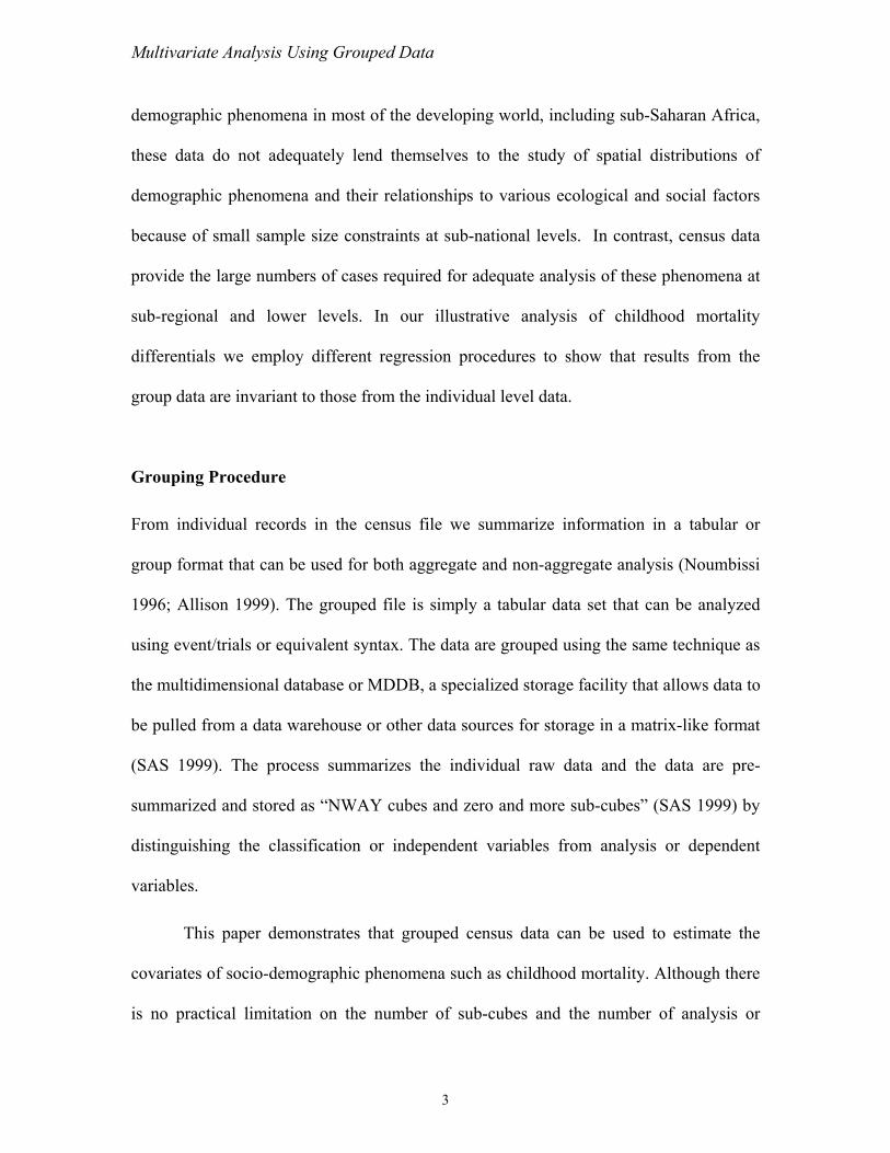
dependent variables, we limit the analysis in this paper to a few variables in order to

facilitate the demonstration. The variables employed are: place of residence (urban or

and mother’s

les for the

interest,, the

five selected

independent variables, we created a file containing 2026 records and five variables (see

an extract from the data table in Table 1).

le 1 mp e bt fro nsu cro-data

rural), province or region of residence, level of education, marital status,

age. From the census micro-data we create a data table of independent variab

total number of women who possess the characteristics or attributes of

number of children ever born, and the number who have died. With the

Tab : Exa le of the type of r cords o ained m ce s mi

15-19 Urba a 3 68 187 n No Education Married Lusak 180 11




Age

group

Residence Education Marital

status

Province Number

of women

Children

ever born

Children

dead

35-39 Urban No Education Married Lusaka 3687 19925 3361

40 04 -44 Urban No Education Married Lusaka 3864 23354 47

45-49 Urban No Education Married Lusaka 3064 18748 4313

We group mother’s age, the first variable, into seven five-year age categories. The

second variable, place of residence has two values, urban and rural; while the third

variable, level of education completed, has four values corresponding to no education,

primary, secondary, and college or higher level. The fourth variable, marital status, has

five values (never married, currently married, divorced, separated, and widowed); and the

4


last variable, province of residence, has nine values corresponding to eight provinces of

the country and Lusaka, the main city itself constituting one region that is 16.7 percent

4*5*9=2520;

variables do not have values in some cells, the actual

gro

lier, grouping

the data in this form reduces substantially the number of records in the file, which

reduces computing time for statistical analysis and allows data analysis over the Internet.

Thi e populations

s of African

he analysis in

this paper demonstrates that even without access to the actual individual-level micro-data,

it is possible to estimate demographic events accurately with the grouped or tabular data

tional census.

inear models,

een variables.

hroughout the paper. The variables were chosen from

those typically found in African census data. They are not an exhaustive list of covariates

that might affect mortality. Our choice of variables is meant to be illustrative of the type

of analysis associated with child mortality.

rural and 83.3 percent urban. The expected number of records is 7*2*

however, because some of the

uping yielded 2026 records.

What is the advantage of grouping data in this form? As noted ear

s is especially advantageous when using census micro-data, where whol

are enumerated and often involve millions of records.

More importantly, grouped data allow us to respect the concern

governments and to maintain confidentiality of their national data. Indeed, t

that can be generated using the individual-level micro-data from the na

Also, by presenting data in this tabular form, it becomes easy to use log-l

factor analysis, or correspondence analysis to examine the relationship betw

We used a simple set of variables t

5


An Illustration with Multivariate Mortality Analysis

Over the past 25 years, Brass-type estimates of childhood mortality in developing

972; Trussell

aus routinely

retrospective

births and the

survival status of the resulting children. While census bureaus tend to use such estimates

to examine mortality trends, they are also important for understanding differentials in

regarding the

ild mortality.

e of maternal

education for child mortality in Ibadan (Caldwell 1979). Other researchers have also

used the Brass-type questions collected in African censuses to investigate childhood

and Preston

howing large

y, Hamid and

ifferentials of

infant and child mortality among the regions of Egypt by sex and socioeconomic status.

They discovered large variations in the levels and differentials of infant and child

mortality in the country, with those in Upper Egypt having the highest probabilities of

dying. A 15-country study by the United Nations (1985) also estimated socioeconomic

differentials in childhood mortality noting differences within different social and

countries have become standard procedures (Brass et al. 1968; Sullivan 1

1975; Preston and Palloni 1977; Trussell and Preston 1982). Census bure

make and report such estimates. These census estimates are based upon

reports given by women regarding their past cumulative number of live

child mortality.

Brass-type analyses have been the basis of several studies

relationship of social and economic factors associated with levels of ch

Caldwell used such a strategy in his multivariate analysis of the importanc

mortality differentials in Africa. Using the 1976 Sudan census data, Farah

(1982) for instance, estimated child mortality differentials in the Sudan, s

differences between the northern and southern parts of the country. Similarl

Ahmed (1988) estimated the levels, trends (from 1976 to 1986), and d

6


economic groups, both within and between countries. Using the 1900 and 1910 United

States census data, Preston and Haines (1991) estimated historical mortality differences

betw .

iate statistical

ass-type data

community).

These authors compared various statistical models for estimating the association between

childhood mortality and socioeconomic and cultural characteristics of the family,

ical evidence

assumed that

g the same

indexes that require the selection

of a mortality standard for their computation. Their indexes are incorporated into a

regression model to estimate the covariates of childhood mortality.

deaths (Oi) to

men based on

; Preston and

(WLS) or the

Tobit regression model. For the WLS regression, Preston and Haines (1991) suggest the

as a weight. The Tobit model is recommended

when the dependent variable is truncated or bounded, as is the case with the Trussell and

Preston Mortality Index (Trussell and Preston 1982).

een different social, income, and racial groups at the turn of the century

Trussell and Preston (1982) provide the first review of multivar

procedures for estimating the association between child mortality from Br

and various social and economic processes (i.e., family, household, and

household, and community in which the child is born. Considering empir

from the analysis of sets of model life tables, Trussell and Preston (1982)

the patterns of mortality should be unique for individuals possessin

characteristics. They then proposed a series of mortality

The Mortality Index is computed based on the observed number of

women of a certain age and the expected number of deaths (Ei) to those wo

the pattern of mortality from a selected standard (Trussell and Preston 1982

Haines 1991).1 They suggested either the use of weighted least squares

use of the number of children ever born

1-- For an evaluation of these indexes, see Noumbissi (1996).

7


In our analysis, we considered different models using both the grouped and the

ungrouped data, including those recommended by Trussell and Preston (1982). We

review below the different models used in this paper.

The Tobit model is defined using the following equation as a latent variable:

ik are a set of K dummy

independent variables measured on the ith woman. Using this latent variable, a censored

random variable ki is defined as followed:

hed by Brass

bit models to

estimate the covariates of mortality from both grouped and ungrouped data. Brass (1975)

used standard mortality and fertility models and established that the proportion of

children dead for women aged x at the time of census or survey (Dx) is approximately

equal to the probability of dying from birth to age ax (ax ranging from 0 to x–α):

0k ifk ** >= iiik

The Tobit Model

Where k* is the estimated morta

iikkiii ezzzk +++++= ββββ ...22110*

lity index and Zi1, Zi2… Z

The Logit, Complementary Log-Log, and Probit Models

We also propose a simplified procedure based on the relationship establis

(1975) that allows the use of either the logit, complementary log-log, or pro

0k if0 * == iik

8


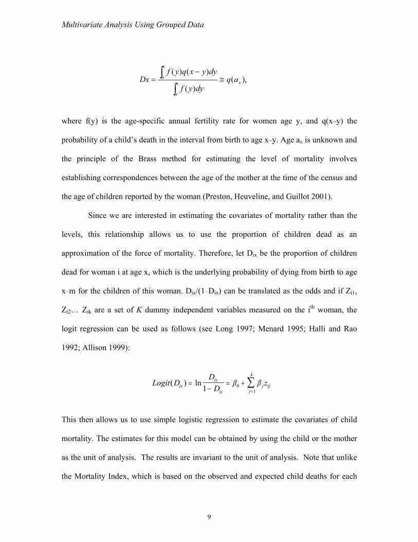
where f(y) is the age-specific annual fertility rate for women age y, an

probability of a child’s death in the interval from birth to age x–y. Age a is u

),()(

)()(xx

x

aqdyyf

dyyxqyfDx ≅

−=

∫∫

α

α

d q(x–y) the

x nknown and

the principle of the Brass method for estimating the level of mortality involves

establishing correspondences between the age of the mother at the time of the census and

the age of children reported by the woman (Preston, Heuveline, and Guillot 2001).

ather than the

dead as an

ix n of children

dead for woman i at age x, which is the underlying probability of dying from birth to age

x–m for the children of this woman. Dix/(1–Dix) can be translated as the odds and if Zi1,

Zi2… Zik are a set of K dummy independent variables measured on the ith woman, the

logit regression can be used as follows (see Long 1997; Menard 1995; Halli and Rao

1992; Allison 1999):

This then allows us to us variates of child

mortality. The estimates for this model can be obtained by using the child or the mother

as the unit of analysis. The results are invariant to the unit of analysis. Note that unlike

the Mortality Index, which is based on the observed and expected child deaths for each

Since we are interested in estimating the covariates of mortality r

levels, this relationship allows us to use the proportion of children

approximation of the force of mortality. Therefore, let D be the proportio

Logit D zix j ij( ) ln=−

= + ∑0β βD

Dix

ix j

k

=1 1

e simple logistic regression to estimate the co

9


woman, our estimates are based on the survival status of each child. We create a

dichotomized variable (children dead and children surviving) as the dependent variable,

and

. The logistic

of assuming

ay assume the Gompertz distribution and

use the complementary log-log models defined as follow:

use the logistic model to estimate the covariates of childhood mortality.

Each of the estimated models assumes a pattern of underlying errors

regression assumes that this pattern follows a logistic distribution. Instead

that the errors have logistic distribution, one m

∑=

umes that the errors have a normal

distribution with a conditional mean of zero and a variance of one (Long 1997).

Following this assumption the probit model is defined as follow:

φ–1 probit) of a

standard normal variable (Allison 1999).

The Negative Binomial Model

ildren born or

dead—it is possible to use the negative binomial regression model, which is based on

count data. The negative binomial model is a generalization of the Poisson regression

model and is better suited to handling observed and unobserved heterogeneity among

individuals (Long 1997). The number of children dead for each woman (yi) should have a

Poisson distribution with a conditional mean (λi) that depends on individual observed

(Zi1, …Z2k) and unobserved (gI) characteristics. Since the conditional mean λi depends

+=−−=k

jzDDC

1))1ln(ln()log(log ββ

We also employ the probit model, which ass

ijjixix 0

∑=

− +=j

ijjix zD1

01 )( ββφ

k

where is the inverse of the cumulative distribution function (called

Considering the questions asked in the census—a count of the number of ch

10


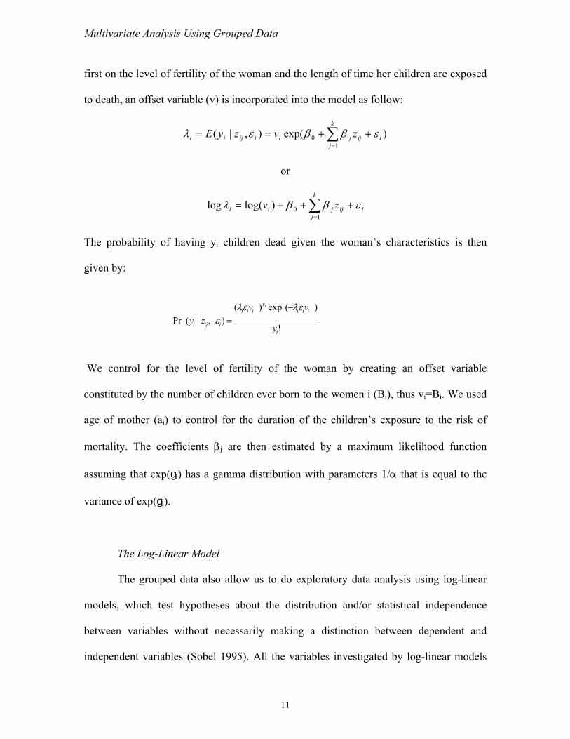
first on the level of fertility of the woman and the length of time her children are exposed

to death, an offset variable (v) is incorporated into the model as follow:

or

The probability of having yi children dead given the woman’s characteristics is then

given by:

We control for the level of fertility of the woman by creating an offset variable

constituted by the number of children ever born to the women i (Bi), thus vi=Bi. We used

age of mother (ai) to control for the duration of the children’s exposure to the risk of

mortality. The coefficients βj are then estimated by a maximum likelihood function

assu s a gamma distribution with parameters 1/α that is equal to the

var

The Log-Linear Model

The grouped data also allow us to do exploratory data analysis using log-linear

models, which test hypotheses about the distribution and/or statistical independence

between variables without necessarily making a distinction between dependent and

independent variables (Sobel 1995). All the variables investigated by log-linear models

)exp(),|(1

0 i

k

jijjiiijii zvzyE εββελ ++== ∑

=

iijjii zv εββλ +++= ∑0)log(log k

j=1

),|(Pri

iiiiii

zy ε =!

)(exp)( y

iiji y

vv i ελελ −

ming that exp(gI) ha

iance of exp(gI).

11


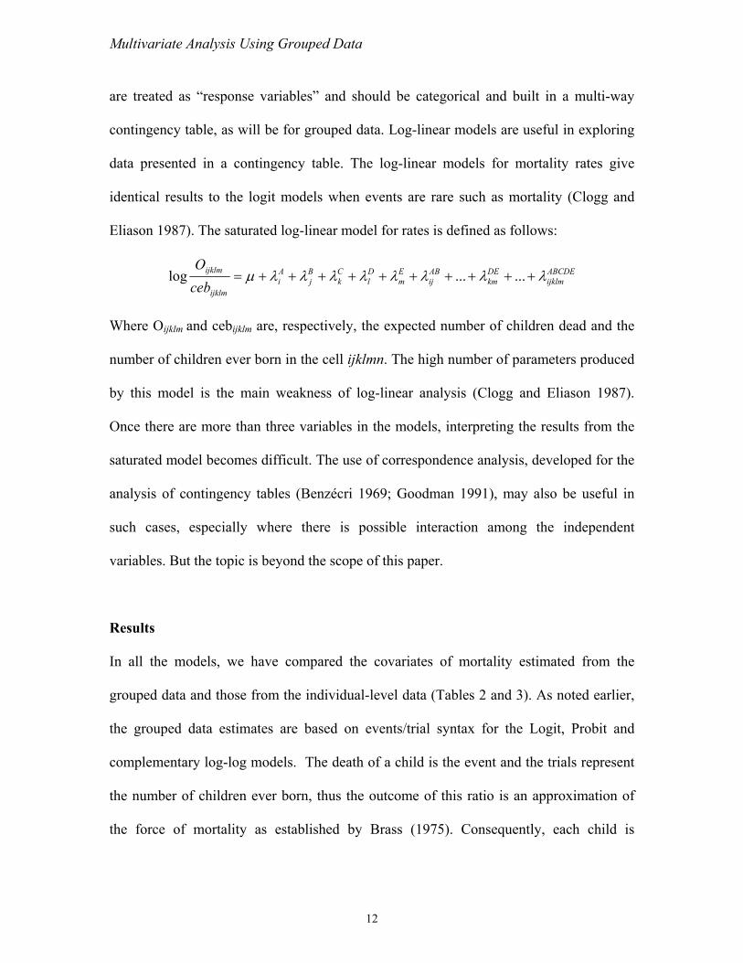
are treated as “response variables” and should be categorical and built in a multi-way

contingency table, as will be for grouped data. Log-linear models are useful in exploring

ity rates give

as mortality (Clogg and

Eliason 1987). The saturated log-linear model for rates is defined as follows:

data presented in a contingency table. The log-linear models for mortal

identical results to the logit models when events are rare such

klmijklm

ijklmO ABCDE

ijDEkm

ABij

Em

Dl

Ck

Bj

Aiceb

λλλλλλλλµ ++++++++++= ......log

ijklm ijklm

number of children ever born in the cell ijklmn. The high number of parame

by this model is the main weakness of log-linear analysis (Clogg and E

Once there are more than three variables in the models, interpreting the re

saturated model becomes difficult. The use of correspondence analysis, deve

Where O and ceb are, respectively, the expected number of children dead and the

ters produced

liason 1987).

sults from the

loped for the

analysis of contingency tables (Benzécri 1969; Goodman 1991), may also be useful in

such cases, especially where there is possible interaction among the independent

the

grouped data and those from the individual-level data (Tables 2 and 3). As noted earlier,

the grouped data estimates are based on events/trial syntax for the Logit, Probit and

complementary log-log models. The death of a child is the event and the trials represent

the number of children ever born, thus the outcome of this ratio is an approximation of

the force of mortality as established by Brass (1975). Consequently, each child is

variables. But the topic is beyond the scope of this paper.

Results

In all the models, we have compared the covariates of mortality estimated from

12


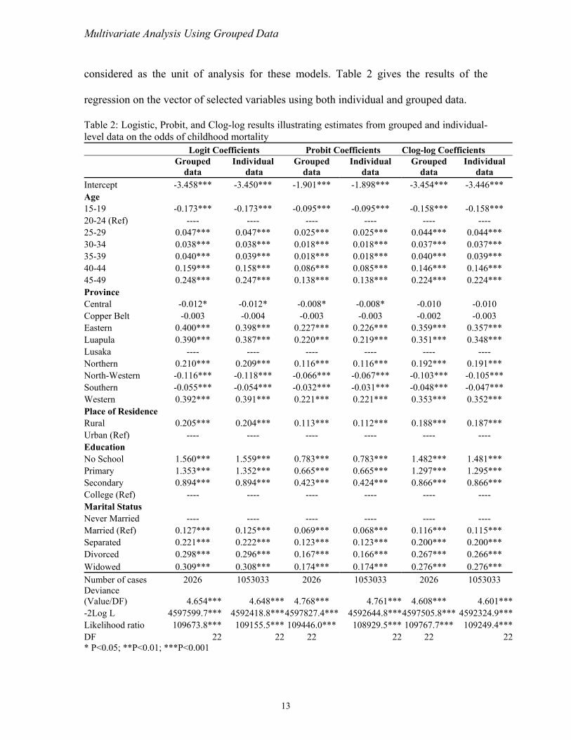
considered as the unit of analysis for these models. Table 2 gives the results of the

regression on the vector of selected variables using both individual and grouped data.

Table 2: Logistic, Probit, and Clog-log resu tim and individual-level data on the odds of ch rt

Logit ficients Probit Coeffic C Coefficients

lts illustrating es ates from groupedildhood mo ality

Coef ients log-logGr ed In vidual rouped Individua Group

Intercept 58* .4 -1 -3.446*** -3.4 ** -3 50*** .90 * 1** -1.898*** -3.454***Age

9 * 0.17 -0 -0.158*** 24 (Ref) ---- -- ----

9 47* 0.04 0. ** 0.044*** 4 38* 0.03 0. ** 0.037***

040** 0.039 0.0 0 * *** 0.039*** .159** 0.158 0.0 0 * *** 0.146***

48* 0.24 0. ** 0.224*** ince

tral -0.012* -0.012* -0.0 -0 * 10 -0.010 .00 -0. - 2 -0.003 00* .39 0. ** 0.357***

ula 90* 0.38 0. ** 0.348*** ---- ---- ---- ---- ---- ----

rthern 10* 0.20 0. ** 0.191*** estern -0.116*** -0.118* -0.06 -0. 3*** -0.105***

n -0.055*** -0.054*** -0.032 ** -0.031*** - *** -0.047*** n 92* 0.39 0. ** 0.352*** f Residen

0.205*** 0.204* 0.11 0. ** ** 0.187*** ---- ---- --- - ---- ----

l 60* 1.55 0. ** 1.481***

y 53* 1.35 0. ** 1.295*** dary 94* 0.89 0. ** 0.866***

---- ---- ---- atus

arried -- -- --- ---- ied (Ref) 7 0 0.115***

1* 0. 0.200*** 98*** 0.296*** 0.167*** 0.166*** 0.267*** 0.266***

Wid wed 0.309*** 0.308*** 0.174*** 0.174*** 0.276*** 0.276*** Number of cases 2026 1053033 2026 1053033 2026 1053033

15-1 -0.173 ** - 3*** .095*** -0.095*** -0.158***20- -- ---- ---- ----25-2 0.0 ** 7*** 025*** 0.025*** 0.044*30-3 0.0 ** 8*** 018*** 0.018*** 0.037*35-39 0. * *** 18*** .018** 0.04040-44 0 * *** 86*** .085** 0.14645-49 0.2 ** 7*** 138*** 0.138*** 0.224*Prov Cen 08* .008 -0.0Copper Belt -0 3 004 0.003 -0.003 -0.00Eastern 0.4 ** 0 8*** 227*** 0.226*** 0.359*Luap 0.3 ** 7*** 220*** 0.219*** 0.351*Lusaka No 0.2 ** 9*** 116*** 0.116*** 0.192*North-W ** 6*** 067*** -0.10Souther * 0.048Wester 0.3 ** 1*** 221*** 0.221*** 0.353*Place o ce Rural ** 3*** 112* 0.188*Urban (Ref) - --- Education No Schoo 1.5 ** 9*** 783*** 0.783*** 1.482*Primar 1.3 ** 2*** 665*** 0.665*** 1.297*Secon 0.8 ** 4*** 423*** 0.424*** 0.866*College (Ref) ---- ---- ----Marital StNever M -- -- - ---- ---- Marr 0.12 *** 0.125*** .069*** 0.068*** 0.116***Separated 0.22 ** 0.222*** 123*** 0.1 ** 23* 0.200***

oup

data di data

Gdata

l data

ed data

Individual data

Divorced 0.2o

Deviance (Value/DF) 4.654*** 4.648*** 4.768*** 4.761*** 4.608*** 4.601***-2Log L 4597599.7*** 4592418.8***4597827.4*** 4592644.8***4597505.8*** 4592324.9***Likelihood ratio 109673.8*** 109155.5*** 109446.0*** 108929.5*** 109767.7*** 109249.4***DF 22 22 22 22 22 22* P<0.05; **P<0.01; ***P<0.001

13


Results from the grouped data reproduce exactly the same estimates as those

obtained from the individual-level data. Slight differences occur however, in the

(B=0) is the

ce is slightly

ata estimates.

, are invariant

to grouping insofar as the groupings are identical with respect to the variables in the

model (Allison 1999). Allison (1999) argues that the deviance based on grouped data is

ul as a goodness-of-fit measure than the deviance based on individual-level

data a chi-square

ncy tables or

grouped data have a log-linear model that is exactly equivalent (see Figure 1). Because

log-linear models have more potential for analysis, grouping census micro-data in the

odels to test

variables with

ining causal theories. This may also be extended to the use of the

correspondence analysis developed for the analysis of contingency tables, and may

complement regression analysis in cases of suspected interaction and association among

independent variables.

goodness-of-fit statistics. While the –2log L used to test the null hypothesis

same for both the grouped and individual-level micro-data, the devian

smaller in the case of the individual-level estimates compared to the group d

Maximum likelihood estimates, their standard errors and the log-likelihood

more “usef

because the deviance from the individual-level data does not have

distribution.”

As noted earlier, the logit, probit and clog-log models for continge

form proposed here allows us to explore the data using log-linear m

hypotheses about the distribution and/or statistical independence between

the aim of exam

14


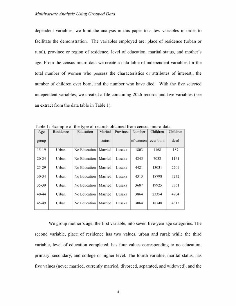
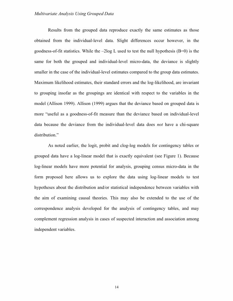
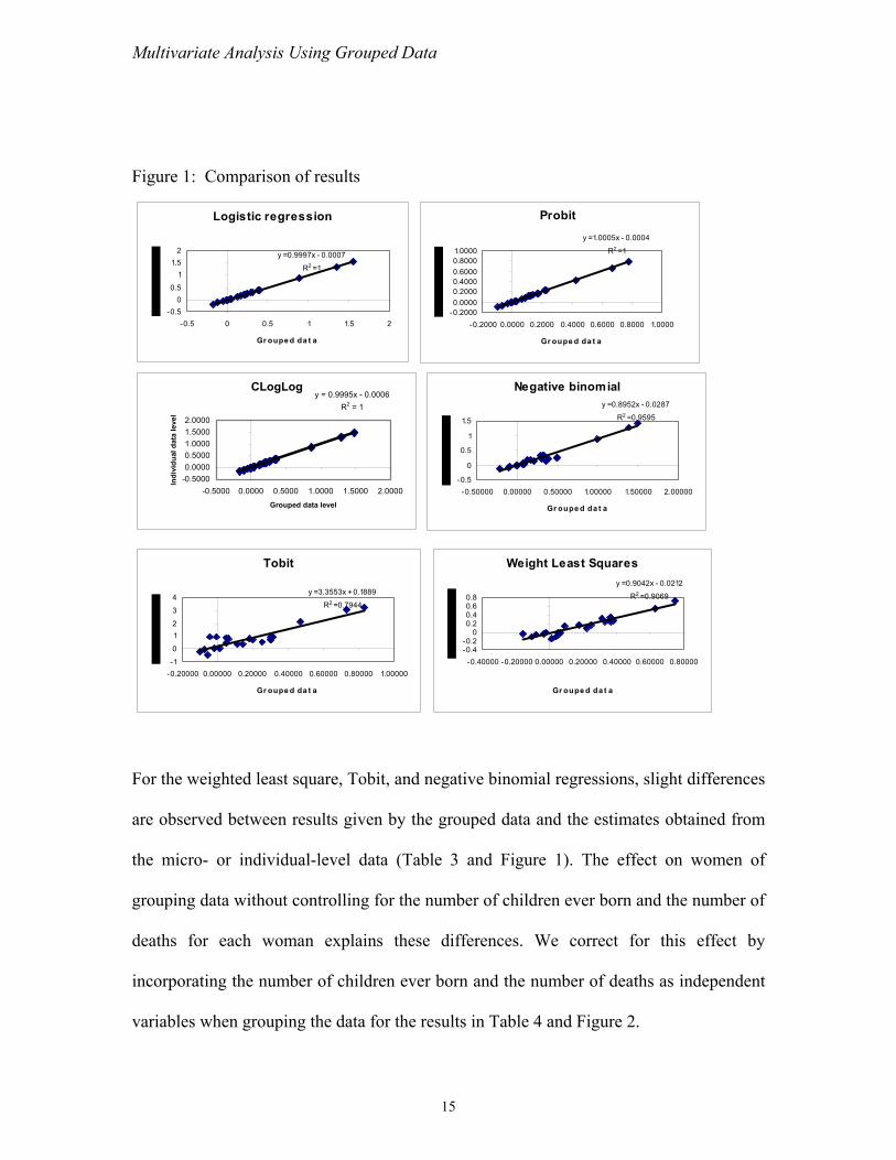
Figure 1: Comparison of results

Logistic regression

y = 0.9997x - 0.0007

R2 = 1

-0.50

0.5

11.5

2

-0.5 0 0.5 1 1.5 2

Gr oupe d da t a

Probity = 1.0005x - 0.0004

R2 = 1

-0.20000.00000.20000.40000.60000.80001.0000

-0.2000 0.0000 0.2000 0.4000 0.6000 0.8000 1.0000

Gr oupe d da t a

CLogLog

y = 0.9995x - 0.0006R2 = 1

-0.50000.00000.50001.00001.50002.0000

-0.5000 0.0000 0.5000 1.0000 1.5000 2.0000Grouped data level

Indi

vidu

al d

ata

leve

l

Negative binomialy = 0.8952x - 0.0287

R2 = 0.9595

-0.5

0

0.5

1

1.5

-0.50000 0.00000 0.50000 1.00000 1.50000 2.00000

Gr oupe d da t a

Tobit

y = 3.3553x + 0.1889

R2 = 0.7944

0

12

3

4

Gr oupe d da t a

Weight Least Squaresy = 0.9042x - 0.0212

R2 = 0.9069

-0.4-0.2

00.20.40.60.8

0.80000

Gr oupe d da t a

-1-0.20000 0.00000 0.20000 0.40000 0.60000 0.80000 1.00000

-0.40000 -0.20000 0.00000 0.20000 0.40000 0.60000

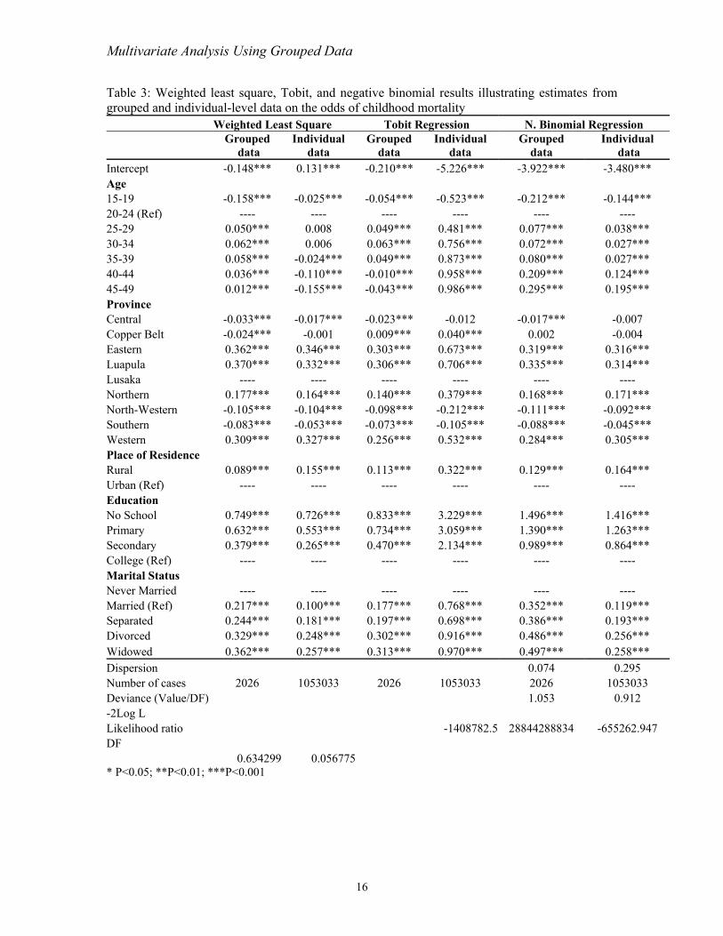
For the weighted least square, Tobit, and negative binomial regressions, slight differences

are observed between results given by the grouped data and the estimates obtained from

the micro- or individual-level data (Table 3 and Figure 1). The effect on women of

grouping data without controlling for the number of children ever born and the number of

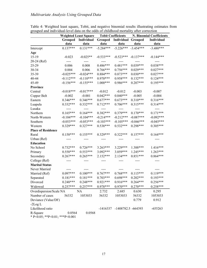
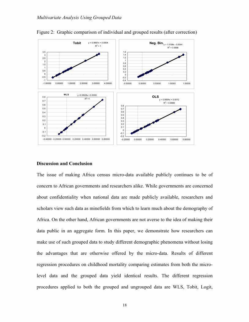
deaths for each woman explains these differences. We correct for this effect by

incorporating the number of children ever born and the number of deaths as independent

variables when grouping the data for the results in Table 4 and Figure 2.

15


Table 3: Weighted least square, Tobit, and negative binomial results illustrating estimates from grouped and in n the o morta

ht u gre ial Regression dividual-level data o dds of childhood lity

Weig ed Least Sq are To t Rebi ssion N om. BinGr

dped a

In ividual ata

rouped data

dividual data

Groupeddata

Intercept 48 .1 -0 - -3.480*** -0.1 *** 0 31*** .210*** 5.226*** -3.922***Age

9 * -0.0 -0 -0 -0.144*** 24 (Ref) ---- - ---- 29 0 0. 0. 0. 0.038*** 34 2 0. 0. 0. 0.027***

0.058*** -0.024*** 0.049 0.873 ** 0.080*** 0.027*** 4 36 .1 -0.0 0 0 * 0.124***

12* -0.1 -0 0.9 0 * 0.195*** ince al 0.0 -0 -0.007

-0 0 0 -0.004 62 .3 0 0 0.316***

la 70 .3 0 0 0.314*** a --- - ----

0.177*** 0.164*** 0.140 0.379 ** 0.168*** 0.171*** estern 0.1 -0 -0 -0.092***

n -0.083*** -0.053*** -0.073 ** -0.105 -0.088*** -0.045*** n 09 .3 0 0 0.305***

of Residenc 89 .1 0 0 0.164***

f) ---- ---- -- - ----

l 49 .7 0 3 1.416*** y 32 .5 0 3 1.263***

dary 79 .2 0 2 0.864*** e (Ref) --- - ---- l Status

ed ---- --- ---- 0.2 *** 0 00*** .177*** 0.7 0 0.119*** 0.2 *** 0.181*** 0.1 0.193***

ivorced 0.3 *** 0 48*** .302*** 0.916 ** 0.486*** 0.256*** Widowed 2*** 57*** .313*** 0.970*** 0.497*** 0.258***

0.074 0.295

15-1 -0.158 ** 25*** .054*** .523*** -0.212***20- --- ---- ---- ---- 25- 0.05 *** 008 049*** 481*** 0.077***30- 0.06 *** 006 063*** 756*** 0.072***35-39 *** *40-4 0.0 *** -0 10*** 10*** .958*** .209**45-49 0.0 ** 55*** .043*** 86*** .295**Prov Centr -0.033*** - 17*** .023*** -0.012 -0.017***Copper Belt -0.024*** .001 .009*** .040*** 0.002 Eastern 0.3 *** 0 46*** .303*** .673*** 0.319*** Luapu 0.3 *** 0 32*** .306*** .706*** 0.335*** Lusak - --- ---- ---- ---- Northern *** *North-W -0.105** -* 04*** .09 * 8** .21 * 2** -0.1 ***11Souther * ***Wester 0.3 *** 0 27*** .256*** .532*** 0.284***Place e Rural 0.0 *** 0 55*** .113*** .322*** 0.129***Urban (Re -- --- ---- Education No Schoo 0.7 *** 0 26*** .833*** .229*** 1.496***Primar 0.6 *** 0 53*** .734*** .059*** 1.390***Secon 0.3 *** 0 65*** .470*** .134*** 0.989***Colleg - --- ---- ---- ---- Marita Never Marri - ---- ---- ---- Married (Ref) 17 .1 0 68 *** .352***Separated 44 97*** 0.698*** 0.386*** D 29 .2 0 *

0.36 0.2 0

ouat

dd

G In Individual data

Dispersion Number of cases 2026 1053033 2026 1053033 2026 1053033 Deviance (Value/DF) 1.053 0.912 -2Log L Likelihood ratio -1408782.5 28844288834 -655262.947 DF 0.634299 0.056775 * P<0.05; **P<0.01; ***P<0.001

16


Table 4: Weighted least square, Tobit, and negative binomial results illustrating estimates from grouped and i n h rrection

ial Coefficients ndividual-level data o the odds of child ood mortality after co

Weight easted L Sq euar T Coobit ef ntsficie N. BinomGr

duped ta

In ividual data

Grouped data

Individu atad

Groupeddata

Intercept 13 . - * * -3.480*** 0. 7*** 0 131*** 5.284*** -5.226** -3.454**Age

9 -0.0 -0 - ** * -0.144*** 24 (Ref) --- ---- 29 0. 0 ** * 0.038*** 34 0. 0 ** * 0.027***

-0.025** -0.024 0.884*** 0. ** 0.0 ** 0.027*** 4 .1 0. ** ** 0.124***

.156 -0. 1 ** ** 0.195*** ince al 1 . -0.007

. - 0 ** -0.004 4 . 0.316***

la 3 . 0.314*** ----

0.165** .164* 0.382*** 0. ** 0.1 ** 0.171*** estern 0 . - ** * -0.092***

n -0.053*** -0.053 -0.10 *** -0 *** -0.046*** -0.045*** n 2 . 0 ** * 0.305***

of Reside 5 . 0 ** * 0.164***

f) ---- -- ----

l 3 . 3 ** * 1.416*** y 5 . 3 ** * 1.263***

dary 6 . 2 ** * 0.864*** e (Ref) -- ----

ed -- - ----

0.0 ** 0 00*** .767*** * ** 0.119*** 0.1 ** 0.1 0 ** 0.193***

ced * 48*** .921*** 0. * 0.264*** 0.256*** ** 0.257*** 0.978*** 0.970*** 0.270*** 0.258***

Overdispersion/Scale NA NA 2.732 2.685 0.630 0.295

15-1 23 .025** 0.533*** -0.523* -0.137**20- - ---- ---- ---- ---- 25- 006 0.008 .486*** 0.481* 0.039**30- 004 0.006 .766*** 0.756* 0.029**35-39 * *** 873* 30*40-4 -0.112*** -0 10*** 970*** 0.958* 0.132*45-49 -0 *** 155*** .000*** 0.986* 0.207*Prov Centr -0.0 8*** -0 017*** -0.012 -0.012 -0.003 Copper Belt -0 002 0.001 .042*** 0.040* -0.005 Eastern 0.3 6*** 0 346*** 0.677*** 0.673*** 0.310***Luapu 0.3 2*** 0 332*** 0.712*** 0.706*** 0.315***Lusaka ---- ---- ---- ---- ---- Northern * 0 ** 379* 70*North-W -0.1 4* -0** 104 *** 0.2 **14* -0 2*.21 -0 7**.08Souther *** 3 .105Wester 0.3 9*** 0 327*** .538*** 0.532* 0.298**Place nce Rural 0.1 8*** 0 155*** .329*** 0.322* 0.157**Urban (Re -- ---- ---- ---- Education No Schoo 0.7 2*** 0 726*** .263*** 3.229* 1.388**Primar 0.5 8*** 0 553*** .092*** 3.059* 1.245**Secon 0.2 7*** 0 265*** .152*** 2.134* 0.851**Colleg -- ---- ---- ---- ---- Marital Status Never Marri -- --- ---- ---- ---- Married (Ref) 97* .1 0 0.7 8*6 * 0.115*Separated 81* 81*** .703*** 0.698* 0.202***Divor 0.248* * 0.2 0 916**

oa

d al

Individual data

Widowed 0.257*

Number of cases 56332 1053033 56332 1053033 56332 1053033 Deviance (Value/DF) 0.779 0.912 -2Log L Likelihood ratio -1416337 -1408782.5 -664393 -655263 R-Square 0.0564 0.0568 * P<0.05; **P<0.01; ***P<0.001

17


Figure 2: Graphic comparison of individual and grouped results (after correction)

Tobit y = 0.9897x + 0.0004R2 = 1

-1-0.5

00.5

11.5

22.5

33.5

-1.00000 0.00000 1.00000 2.00000 3.00000 4.00000

Neg. Bin.y = 1.0196x - 0.0044R2 = 0.9998

-0.4-0.2

00.20.40.60.8

11.21.41.6

-0.50000 0.00000 0.50000 1.00000 1.50000

y = 0.9928x + 0.0008

R2 = 1

-0.2

-0.1

0

0.1

0.2

0.3

0.4

0.5

0.6

0.7

0.8

0.40000 0.60000 0.80000

WLSOLS

y = 0.9954x + 0.0012R2 = 0.9999

-0.2-0.1

00.10.20.30.40.50.60.70.8

-0.20000 0.00000 0.20000 0.40000 0.60000 0.80000

-0.40000 -0.20000 0.00000 0.20000

concern to African governments and researchers alike. While governments

about confidentiality when national data are made publicly available, res

scholars view such data as minefields from which to learn much about the d

Africa. On the other hand, African governments are not averse to the idea of

Discussion and Conclusion

The issue of making Africa census micro-data available publicly continues to be of

are concerned

earchers and

emography of

making their

data public in an aggregate form. In this paper, we demonstrate how researchers can

make use of such grouped data to study different demographic phenomena without losing

the advantages that are otherwise offered by the micro-data. Results of different

regression procedures on childhood mortality comparing estimates from both the micro-

level data and the grouped data yield identical results. The different regression

procedures applied to both the grouped and ungrouped data are WLS, Tobit, Logit,

18


Probit, Complementary log log, and Negative Binomial regression models. Each of these

procedures relies on different assumptions.

The Trussell and Preston Mortality Index uses the observed numb

ever born and the number of children surviving over the expected number of

dependent variable. The negative binomial regression uses a count of t

deaths as the dependent variable. Both the Trussell and Preston Mortality

included in the model. On the other hand, the grouped data are expecte

estimate with less unobserved variation because the same explanatory var

reflect the averaging influence of the larger group. The results for the i

grouped data are invariant in that the estimates are identical with respect to

results. Initial differences observed between the grouped and

er of children

deaths as the

he number of

Index and the

negative binomial regression use a dependent variable in the individual-level analysis that

can be expected to reflect the idiosyncratic variation unaccounted for by the variables

d to yield an

iables tend to

ndividual and

the nature of

the variables. In the case where the idiosyncratic nature of the individual-level results

has a significant impact on the estimation, we should expect to observe differences in the

individual results for the

WL valence in the

y controlling

The grouped file reduces the concern of some African governments regarding the

confidentiality of census micro-data and produces results identical to those obtained

using the actual individual-level micro-data. For the purposes of our demonstration we

use the national census of Zambia collected in 1990 and selected only five variables often

associated with childhood mortality. The selection of the variables is not meant to

S, Tobit, and negative binomial regressions result from the lack of equi

offset variable for the two forms of data. We adjusted for these differences b

for the number of children ever born and the number of surviving children.

19


provide an exhaustive list of factors affecting mortality, but is illustrative of variables

considered important and available in African census data.

As shown in Tables 2 and 3 the results from the different models n

but also confirm our expectations and are consistent with the literature.

among the five variables selected for demonstration, maternal education app

most important factor associated with childhood mortality. This is consiste

Caldwell 1979; United Nations 1985; Cleland, Bicego and Fegan 1992). Be

women often have better access to resources, both material and human cap

them to ha

ot only agree,

For example,

ears to be the

nt with earlier

research (Farah and Preston 1982; Hobcraft, McDonald, and Rutstein 1984; Cleland and

van Ginneken 1988; Cochrane, O’Hara, and Leslie 1980; Tabutin and Akoto 1992;

tter educated

ital, allowing

ve a comparative advantage in providing better health for their children

(Cl 1984; United

Nations 1985).

With regard to marital status, the odds of child mortality are lower for children of

other factors.

ed) children

d women have better survival chances, which is consistent with the literature.

We of the never

married, but we believe that other factors might be important in explaining these

differences.

The regions with the highest childhood mortality are the Eastern, Luapula,

Western, and the Northern regions, compared to the Copper Belt, Central, and Lusaka

regions, which reportedly have an intermediate level of childhood mortality. North-

eland and van Ginnekan 1988; Hobcraft, McDonald, and Rutstein

nonmarried women than all other marital groups, even when we control for

However, compared to the remaining groups (separated, divorced, and widow

of marrie

do not fully investigate the reason behind the advantage for children

20


Western and Southern provinces appear to have the lowest mortality (Central Statistical

Office 1990). As expected, childhood mortality is higher in rural areas than in urban

areas. Finally, the age effect for the Logit, Probit, Complementary log-log

binomial models also follows the expected pattern, except among the 15

, and negative

-19-year-old age

gro lot 2001).

estimation of

the covariates of childhood mortality, the procedures can easily be applied to other- social

phenomena. Considering that researchers are rarely given the census micro-data, this

dem do regression

data.

h will allow

rtake detailed

multivariate regression analysis. Theoretically there will be no limitation on the number

of dependent variables since the procedure uses the multidimensional database (MDDB)

This storage system allows data to be pulled from a data warehouse or other

source for storage in a matrix-like format (SAS 1999). Thus ACAP can make the

grouped data available to researchers online without violating the concerns of African

governments.

up, which typically produces erratic results (Preston, Heuveline and Guil

Although we demonstrated the application of the procedures with an

onstration shows that it is possible to use grouped census micro-data to

analysis and obtain results identical to those obtained from the actual micro-

ACAP is in the process of grouping African census data whic

researchers to have access to such grouped data and still be able to unde

technique.

21


References

llison, D. Paul. 1999. Logistic RegressA ion Using the SAS System, Theory and

Brass, William et al. 1968. The Demography of Tropical Africa. Princeton, NJ: Princeton

B stimating Fertility and Mortality from Limited and

Defective Data he University

Benzécri J. P. 1969 “Statistical analysis as a tool to make patterns emerge from data,” in

w York: Academic

f

Nigerian data,” Population Studies 33: 395.

C n, Housing and Agriculture Analytical Report, Vol. 10. Lusaka, Zambia.

equalities in childhood mortality: The 1970s to the 1980s,” Health Transition Review Vol. 2.

C . “Maternal education and child survival in developing countries: The search for pathways of influence,” Social Science and

ar analysis,”

rch 16(1): 8-44.

n on health,” nk.

in Sudan,”

view 8: 365. Goodman, L. A. 1991. “Measures, models, and graphical displays in the analysis of

cross-classified data (with discussion),” Journal of the American Statistical Association 86: 1085-1138.

Halli, Shiva S. and Vaninadha K Rao. 1992. Advanced Techniques of Population

Analysis. New York: Plenum Press.

Application. Cary, NC: SAS Institute Inc., 304 p.

University Press.

rass, William. 1975. Methods of E. Laboratories for Population Statistics, Chapel Hill: T

of North Carolina at Chapel Hill, 159 p.

Methodologies of Pattern Recognition, ed. S. Watanabe. NePress, pp. 35-73.

Caldwell, J. C. 1979. “Education as factor in mortality decline: An examination o

entral Statistical Office (Zambia). 1990. Census of Populatio

Cleland, J., George Bicego, and Greg Fegan. 1992. “Socioeconomic in

leland, J. G and J. K van Ginneken.. 1988

Medicine 27(12): 1357-1368.

Clogg, C. C. and S. Eliason. 1987. “Some common problems in Log-LineSociological Methods and Resea

Cochrane, S. H., D. J. O’Hara, and J Leslie. 1980. “The effects of educatioWorld Bank Staff Working Paper No. 405. Washington, DC: World Ba

Farah, A. A. and S. H. Preston. 1982. “Child mortality differentialsPopulation Development Re

22


Hamid, Abd El N. M. and F. A. Ahmed. 1988. “Infant and childhood motrends and differentials, 1986 census,” in Demographic Analysis of Data. Enlarged Sample. Volume II: Nuptiality, Fertility, Mortality aSegments of Population, compiled by Egypt, Central Agency

rtality levels, 1986 Census nd Selected

for Public Mobilisation and Statistics [CAPMAS], Population Studies and Research Centre.

Hobcraft J. N, J. W. McDonald, and S. O. Rutstein. 1984. “Socio-economic factors in

infant and child mortality: A cross national comparison,” Population Studies 38:

ited Dependent

Variables. Thousand Oaks, CA: Sage.

M ression Analysis. Thousand Oaks, CA: Sage.

. Applications

Pr Mortality in Late Nineteenth-Century America. Princeton, NJ: Princeton University Press.

Preston, H. Samuel, P. Heuveline, and M. Guillot. 2001. Demography: Measuring and Modeling Population Process. Oxford: Blackwell Publishers Inc.

Preston, H. S. and A. Palloni. 1977. “Fine tuning Brass-type mortality estimates with data in ages of surviving children,” Population Bulletin of the United Nations, No. 10

SAS Institute Inc. 1999. SAS/MDDB Server Administrator's Guide, Cary, NC: SAS

Sobel, Michael E. 1995. “The analysis of the contingency tables,” in G. Arminger, C. C.

he Social and

Sullivan, J. M. 1972. “Models for the estimation of the probability of dying between birth

and exact age of early childhood,” Population Studies 26 (1): 79-97. Tabutin, D. and E. Akoto. 1992. “Socio-economic and cultural differentials in the

mortality of sub-Saharan Africa,” in Mortality and Society in sub-Saharan Africa, E. van de Walle, G. Pison, and M. Salad-Diakanda (eds.). Oxford: Clarendon Press, pp.32-64.

Cairo: CAPMAS, 165-190.

193.

Long, J. Scott. 1997. Regression Models for Categorical and Lim

enard, Scott. 1995. Applied Logistic Reg

Noumbissi, A. 1996. Méthodologies d’analyse de la mortalité des enfantsau Cameroun. Louvain-la-Neuve: Académia.

eston, H. S. and M. R. Haines. 1991. Fatal Years: Child

pp. 72-91.

Institute Inc.

Clogg, and M. E. Sobel (eds.), Handbook of Statistical Modeling for tBehavioral Sciences. New York: Plenum Press, pp. 251-310.

23


24

T Brass technique for determining childhood survivorship rates,” Population Studies 29(1): 97-107.

T of childhood mortality from retrospective reports of mothers,” Health Policy and Education 3: 1-

United Nations. 1985. Socioeconomic Differentials in Child Mortality in Developing

Countries. ST/ESA/SER. A/97. New York.

russell, J. 1975. “A re-estimation of the multiplying factors for the

russell, James and Samuel Preston. 1982. “Estimating the covariates

36.

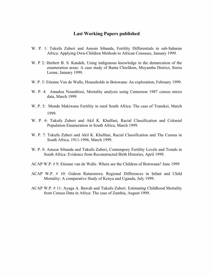
Last Working Papers published

W. P. 1: Tukufu Zuberi and Ansom Sibanda, Fertility Differentials in sub-Saharan

Africa: Applying Own-Children Methods to African Censuses, January 1999. W. P 2: Herbert B. S. Kandeh, Using indigenous knowledge in the demarcation of the

enumeration areas: A case study of Banta Chiefdom, Moyamba District, Sierra Leone, January 1999.

W. P. 3: Etienne Van de Walle, Households in Botswana: An exploration, February 1999. W. P. 4: Amadou Noumbissi, Mortality analysis using Cameroon 1987 census micro

data, March 1999. W. P. 5: Monde Makiwane Fertility in rural South Africa: The case of Transkei, March

1999.

W. P. 6: Tukufu Zuberi and Akil K. Khalfani, Racial Classification and Colonial Population Enumeration in South Africa, March 1999.

W. P. 7: Tukufu Zuberi and Akil K. Khalfani, Racial Classification and The Census in

South Africa, 1911-1996, March 1999.

W. P. 8: Amson Sibanda and Tukufu Zuberi, Contempory Fertility Levels and Trends in South Africa: Evidence from Reconstructed Birth Histories, April 1999.

ACAP W.P. # 9: Etienne van de Walle. Where are the Children of Botswana? June 1999

ACAP W.P. # 10: Gideon Rutaremwa. Regional Differences in Infant and Child Mortality: A comparative Study of Kenya and Uganda, July 1999.

ACAP W.P. # 11: Ayaga A. Bawah and Tukufu Zuberi. Estimating Childhood Mortality from Census Data in Africa: The case of Zambia, August 1999.

Documents

African Census Analysis Project (ACAP) · nts. We use the grouped file to demonstrate how to estimate the covariates of childhood mortality at the individual level using selected