MITSUBISHI ELECTRIC RESEARCH LABORATORIEShttp://www.merl.com

Adjoint-Based Optimization of Displacement VentilationFlow

Nabi, S.; Grover, P.; Caulfield, C.C.

TR2017-086 July 2017

AbstractWe demonstrate the use of the ’Direct-Adjoint-Looping method’ for the identification ofoptimal buoyancy-driven ventilation flows governed by Boussinesq equations. We use theincompressible Reynoldsaveraged Navier-Stokes (RANS) equations, derive the correspondingadjoint equations and solve the resulting sensitivity equations with respect to inlet conditions.We focus on a displacement ventilation scenario with a steady plume due to a line source.Subject to an enthalpy flux constraint on the incoming flow, we identify boundary conditionsleading to ’optimal’ temperature distributions in the occupied zone. Our results show thatdepending on the scaled volume and momentum flux of the inlet flow, qualitatively differentflow regimes may be obtained. The numerical optimal results agree with analytically obtainedoptimal inlet conditions available from classical plume theory in an ’intermediate’ regime ofstrong stratification and two-layer flow.

Building and Environment

This work may not be copied or reproduced in whole or in part for any commercial purpose. Permission to copy inwhole or in part without payment of fee is granted for nonprofit educational and research purposes provided that allsuch whole or partial copies include the following: a notice that such copying is by permission of Mitsubishi ElectricResearch Laboratories, Inc.; an acknowledgment of the authors and individual contributions to the work; and allapplicable portions of the copyright notice. Copying, reproduction, or republishing for any other purpose shall requirea license with payment of fee to Mitsubishi Electric Research Laboratories, Inc. All rights reserved.

Copyright c© Mitsubishi Electric Research Laboratories, Inc., 2017201 Broadway, Cambridge, Massachusetts 02139

Adjoint-Based Optimization of Displacement Ventilation Flow

Saleh Nabi∗ Piyush Grover † C. P. Caulfield ‡

July 21, 2017

Abstract

We demonstrate the use of the ‘Direct-Adjoint-Looping method’ for the identification of optimalbuoyancy-driven ventilation flows governed by Boussinesq equations. We use the incompressible Reynolds-averaged Navier-Stokes (RANS) equations, derive the corresponding adjoint equations and solve the re-sulting sensitivity equations with respect to inlet conditions. We focus on a displacement ventilationscenario with a steady plume due to a line source. Subject to an enthalpy flux constraint on the incom-ing flow, we identify boundary conditions leading to ‘optimal’ temperature distributions in the occupiedzone. Our results show that depending on the scaled volume and momentum flux of the inlet flow, qual-itatively different flow regimes may be obtained. The numerical optimal results agree with analyticallyobtained optimal inlet conditions available from classical plume theory in an ‘intermediate’ regime ofstrong stratification and two-layer flow.

Keywords Direct-Adjoint-Looping method; Displacement ventilation; Forced convection; Line plume;Intermediate regime; Numerical PDE-constrained optimization

∗Mitsubishi Electric Research Labs, Cambridge, MA, USA. Corresponding Author. Email: nabi@merl.com†Mitsubishi Electric Research Labs, Cambridge, MA, USA.‡BP Institute and Department of Applied Mathematics & Theoretical Physics (DAMTP), University of Cambridge, Cam-

bridge, CB3 0EZ, United Kingdom

1

1 Introduction

Nomenclature

D problem domain Ω region of interest

a area α entrainment coefficient

B,Q,W buoyancy, momentum and heatflux

α′, β′ non-dimensional weighting fac-tor in cost function

Cp specific heat β00 coefficient of volumetric expan-sion

d enthalpy flux representative γ weighting factor for temperaturein cost function

D Universal plume constant ζ non-dimensional interface height

g gravitational force θ non-dimensional temperature

Gr Grashof number κ diffusivity

h interface height ν viscosity

k conductivity ρ density

H,L height and length ω height of the region of interest

n, y unit normal and vertical vector J cost function

Pe Peclet number L augmented cost function

P,W,U vector of adjoint, direct and de-sign variables

q′′ heat flux per length Subscripts

Re Reynolds number a adjoint

Ri Richardson number d desired

T, V, p temperature, velocity and pres-sure fields

eff effective

Vr velocity ratio in inlet

Tcomf comfortable temperature p plume

x horizontal coordination ref reference value

y vertical coordination Superscripts

o optimal

Modern buildings contribute close to 40% of total energy consumption in North America, a large fractionof which is used in HVAC [1]. Design of indoor environments has the twin goals of providing optimalthermal comfort while minimizing energy consumption. The complicated dynamics of airflow within the builtenvironment, and its interaction with occupants, electrical devices and the exterior, necessitate developmentof a systematic approach to fulfill the requirements of such a design.

There are various methods to determine air velocity, temperature, relative humidity, and contaminantconcentration in a room, such as computational fluid dynamics (CFD), analytical models, and experimentalmeasurements [2]. The methods help to identify flow regimes with the desired air quality, thermal comfort,and energy consumption. By using such methods in a trial-and-error process, engineers have been able to

2

design HVAC systems to achieve desired conditions in the built environment [3]. However, this process mayinvolve a large number of iterations and rely heavily on a good initial guess of conditions, which requiresprior knowledge and experience. ‘Moreover, there is no guarantee that the final solution is even close tooptimal, in terms of meeting the design objective, and no physical insight is obtained using a trial-and-errorprocess. The formal definition of optimal solution is given in Section 4.

An efficient determination of the design of an HVAC system for a desirable built environment requires asystematic approach that starts with the design objective. The design objective can be expressed in termsof field variables, e.g. air velocity or temperature, representing thermal comfort, energy consumption, airquality, etc, in the whole or a part of the domain in transient or steady state. Recently, there have beenseveral studies that formulate such problems as inverse design problems [3]. Inverse design problems canbe further classified as either ‘backward’ or ‘forward’ methods [3]. Although they have the attraction ofbeing computationally tractable, backward methods such as the quasi-reversibility method [4], the pseudo-reversibility method [5] and the regularized inverse matrix method [6], all suffer from the fact that the flowfield needs to be known prior to the solution. On the other hand, forward methods, such as CFD-basedadjoint methods [7], reduced-order models (ROMs) [8, 9], and genetic algorithm (GA) [10], solve for boththe flow field and the scalar field, and hence have broader applications.

Reduced-order models have also been extensively used to reduce the computational burden in optimizationand control applications [11]. These methods rely on finding appropriate sets of dominant modes in simulationor experimental data. The problem dimension can then be reduced to the number of modes retained in theprocess. Genetic algorithm methods, with either a single objective or multiple objectives, are converselymuch more computationally expensive [3]. Such computational cost can grow even larger if several inputshave also to be determined. However, it is important to remember that the main advantage of GA methodsis that they provide global optimal solutions [10].

In the last two decades, there has been a large amount of research in the area of design optimization of fluiddynamics processes using adjoint-based methods, including shape optimization of airfoils [12], automotivedesign [13], wind turbines [14], and ducted flows [15]. Another related recent development has been the useof nonlinear adjoint optimization techniques to find ‘optimal’, i.e. minimal energy, perturbations that leadto turbulence in pipe and channel flows [16, 17, 18]. However, application of systematic optimization andcontrol to indoor flows has been missing until very recently [19, 20, 21, 22, 7].

In contrast to shape optimization problems in aerodynamics, indoor airflow dynamics optimization isaimed at obtaining optimal boundary actuation that leads to desired airflow temperature and velocity dis-tribution characteristics in the domain of interest [23]. Since the flow is usually in the turbulent regime,numerical optimization using Direct Numerical Simulation (DNS) or Large Eddy Simulation (LES) is notgenerally feasible. This requires the use of Reynolds-Averaged Navier-Stokes (RANS) models, or some otherclosure models to account for interaction between the mean-flow and turbulent eddies. Since the accuracy ofRANS models in indoor flow can vary according to the flow conditions, it is crucial that the optimization re-sults are verified by direct comparison with experimental results, or with previously experimentally-validatedanalytical models of indoor airflow phenomenon. One such class of analytical models are physics-basedreduced-order models for indoor ventilation dynamics [24]. Beginning with seminal work by Baines andTurner [25], there have been several advances in our understanding of mixing and transport in indoor air-flows. Experimentally validated low-order models have been developed for steady [26] and unsteady [27]natural ventilation, ventilation in the presence of time-varying heat sources [28, 29], exchange flow betweenadjacent rooms [30], and general unsteady plume dynamics [31], among other phenomena.

In this paper, we formulate and solve a model test-case problem to determine inlet velocity and tem-perature that optimize a certain cost functional related to maintaining desired temperature distribution inpart of a room, using and demonstrating the utility of the so-called Direct-Adjoint-Looping (DAL) method[16]. The study focuses on the fully turbulent mixed-convection regime, resulting from the presence of aline heat source in addition to forced conditioned air from the inlet. The open source software Open FieldOperation and Manipulation (OpenFOAM) is used as the numerical tool to develop our continuous-adjointbased framework.

While we perform validation of forward simulation (CFD) results by comparing with experimentally

3

validated models (as is customary), the focus of our work is actually on implementation of RANS-basedDAL optimization on buoyancy-driven flows. In that regard, we validate our optimization results, which isan important contribution of this study. Most previous adjoint-based studies have focused on inverse design,and involved synthetic problems where the optimal solution is known a priori, and hence the validation isstraightforward. In our study, the optimal solution is not known a priori, and we validate our numericaloptimal solutions by comparing them to analytically obtained optimal solutions in a flow regime where theanalytical (forward) model is known to be valid. Another novelty of this work lies in the inclusion of enthalpyconstraints on the inlet flow in the optimization problem to better model real-life scenarios. The constrainedoptimization leads to nontrivial modification of optimal solutions as compared to the unconstrained case.This work is a first step towards developing a validated numerical framework for indoor flow optimizationand it lays out a strategy for dealing with more realistic situations.

The rest of the paper is organized as follows. In Section 2, we derive an analytical model for thebuoyancy-driven flow with bottom and top vents in the presence of a line heat source of buoyancy, buildingupon the existing experimentally-validated models for thermal plumes [32]. In Section 3, we study thesystem using RANS simulations, compare the results to the predictions of analytical models, and identifythe regime of validity of those analytical models based on relevant non-dimensional parameters. In Section4, we formulate the optimization problem, and employ the DAL method to solve the problem numerically.Analytical optimization of the reduced-order analytical model derived in Section 2 is also carried out. InSection 5, detailed comparison of the results from numerical and analytical optimization methods is carriedout. We discuss the validity of the RANS based optimization, and the effect of constraints on the optimalsolution. Finally in Section 6, we provide conclusions and sketch out directions for future research.

2 Analytical Model For Displacement Ventilation

The schematic of the model test case problem for the domain D is shown in Fig. 1. The height of the roomis H, the inlet area (divided by the width of the room) is ain, and the source buoyancy flux is B, which isrelated to the heat flux by

B =Wβ00g

ρCp, (1)

where g is the acceleration due to gravity, W is the heat flux, ρ is the fluid density, Cp is the fluid’s specificheat capacity and β00 is the coefficient of volumetric expansion (for ideal gases β00 ≈ 1/T ).

There is one major difference between this setting and the traditional displacement flow for which venti-lation occurs when the dense fluid enters at the bottom and displaces the lighter fluid within the space whichin turn flows out through the openings at the top [26, 33]. We assume that the space, for simplicity chosento be a two-dimensional cavity with bottom and top vents, is subjected to a prescribed inflow provided byan air conditioning unit or a mechanical machine. This is in contrast with earlier studies, where the spaceis connected to an exterior, which in turn is modeled as a large reservoir with fixed temperature, and theinflows and outflows are driven dynamically by (assumed hydrostatic) pressure differences associated withdensity differences between the interior and exterior fluids. Therefore, the inlet temperature and velocity,(Tin, Vin) are design variables for our problem. Equivalently, the inlet volume flux is determined by the de-sign requirements instead of being a function of the temperature difference between the interior and exterior.We are most interested in the range of parameters that lead to a stable strong stratification and an interfacebetween top and bottom layers. We explore such a flow configuration in more detail in the following.

The analytical model is intended to capture the effect of a continuous source of buoyancy (or heat)on temperature stratification. We restrict our attention to isolated sources of buoyancy, and we focus forcomputational convenience on a two-dimensional line plume. Extension to an axisymmetric point source isstraightforward. Using integral methods and the entrainment hypothesis of Taylor, Morton et al. [32] derivedequations for a buoyant plume in stationary unstratified ambient atmosphere. The volume flux within theplume is given by

4

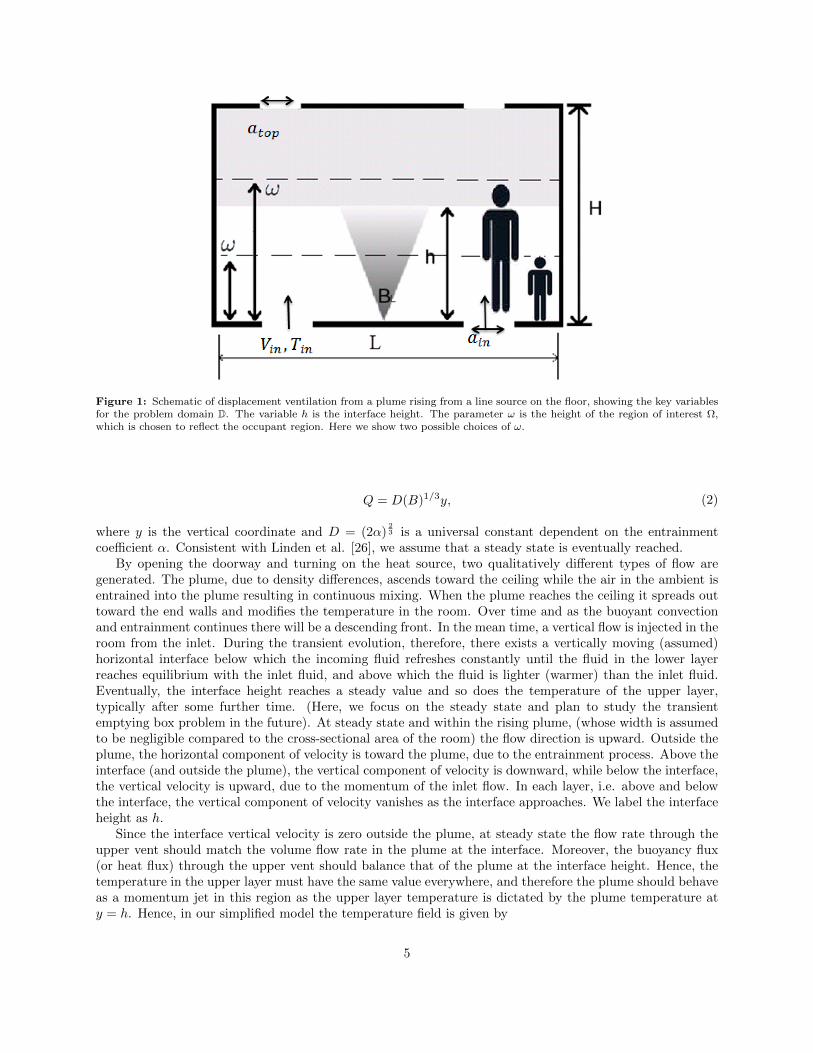
Figure 1: Schematic of displacement ventilation from a plume rising from a line source on the floor, showing the key variablesfor the problem domain D. The variable h is the interface height. The parameter ω is the height of the region of interest Ω,which is chosen to reflect the occupant region. Here we show two possible choices of ω.

Q = D(B)1/3y, (2)

where y is the vertical coordinate and D = (2α)23 is a universal constant dependent on the entrainment

coefficient α. Consistent with Linden et al. [26], we assume that a steady state is eventually reached.By opening the doorway and turning on the heat source, two qualitatively different types of flow are

generated. The plume, due to density differences, ascends toward the ceiling while the air in the ambient isentrained into the plume resulting in continuous mixing. When the plume reaches the ceiling it spreads outtoward the end walls and modifies the temperature in the room. Over time and as the buoyant convectionand entrainment continues there will be a descending front. In the mean time, a vertical flow is injected in theroom from the inlet. During the transient evolution, therefore, there exists a vertically moving (assumed)horizontal interface below which the incoming fluid refreshes constantly until the fluid in the lower layerreaches equilibrium with the inlet fluid, and above which the fluid is lighter (warmer) than the inlet fluid.Eventually, the interface height reaches a steady value and so does the temperature of the upper layer,typically after some further time. (Here, we focus on the steady state and plan to study the transientemptying box problem in the future). At steady state and within the rising plume, (whose width is assumedto be negligible compared to the cross-sectional area of the room) the flow direction is upward. Outside theplume, the horizontal component of velocity is toward the plume, due to the entrainment process. Above theinterface (and outside the plume), the vertical component of velocity is downward, while below the interface,the vertical velocity is upward, due to the momentum of the inlet flow. In each layer, i.e. above and belowthe interface, the vertical component of velocity vanishes as the interface approaches. We label the interfaceheight as h.

Since the interface vertical velocity is zero outside the plume, at steady state the flow rate through theupper vent should match the volume flow rate in the plume at the interface. Moreover, the buoyancy flux(or heat flux) through the upper vent should balance that of the plume at the interface height. Hence, thetemperature in the upper layer must have the same value everywhere, and therefore the plume should behaveas a momentum jet in this region as the upper layer temperature is dictated by the plume temperature aty = h. Hence, in our simplified model the temperature field is given by

5

T =

Tin y ≤ hTp|y=h = Tin + kLh

−1 y > h, (3)

where Tp is the plume temperature, and kL =TrefB

2/3

gD. Eq. (3) implies that at the lower layer the

temperature matches that of the inlet, and at the upper layer it equals that of the plume at the interfaceheight to ensure buoyancy (energy) conservation.

Equating the inlet volume flux per width Qin = ainVin we find the interface height to be

h =

(Qin

DB1/3

). (4)

In contrast to the results of Ref. [26], our model predicts that for specified inlet conditions, the interfaceheight is a function of the source strength B, although it is possible to show that Eqs. (3) and (4) areconsistent with the results of Ref. [26] in the limit of exchange with exterior. Finally, we define an effectivearea (per unit length), a∗in, as

a∗in =ainatop√

0.5(a2top + a2

in).

(5)

Although there is no explicit appearance of a∗in in (4), nevertheless we express the results in following sectionsin terms of this effective area to be consistent with previous dynamically-driven interior/exterior studies. Inderiving our model we assume an incompressible flow where the temperature disparities are small so thatthe Boussinesq approximation holds. The flow is inviscid and the diffusion in the scalar transport equationcan be ignored. The ambient stratification remains stable with increasing temperature from bottom to top.The flow within the plume is assumed to be one-dimensional and in vertical direction. The horizontal flowobeys the Taylor hypothesis for the entrainment [32].

3 Numerical Solution : Validation and Flow Regimes

In this section, we discuss the details of numerical solution of the mixed-convection problem introduced inthe last section, and provide a comparison of our numerical results with experimentally-verified analyticalsolutions.

3.1 Governing equations

The internal flow is governed by the Boussinesq equations:

∇.V = 0,

(V.∇)V +∇p− β00g(T − Tref )y − νeff∇2V = 0,

V.∇T − κeff∇2T = 0,

(6)

where V = (V1, V2) is the fluid velocity, T is the temperature, and y is the unit vector in the vertical direction.Here, the flow is characterized by the parameters νeff and κeff , the effective viscosity and diffusivity, whichcan accommodate eddy viscosity turbulence models. In this study, we use the Reynolds Averaged-Navier-Stokes (RANS) formulation to calculate νeff and κeff . We use the standard k − ε closure model [34] andhence, all the variables in Eq. 6 are mean (time-averaged) values.

We select the two-variable turbulence models since they have been validated for indoor environment [2],and are also computationally feasible. In this study, our focus is on statistically steady ventilation problems.

6

We note that other computational frameworks, such as Large Eddy Simulation (LES) models, are alsopopular for built environment simulation. However, our extensive validation via comparison of numericalresults with analytical plume models, and that of frozen-turbulence based RANS optimization with finite-difference sensitivities, gives us confidence that our choice of turbulence models is appropriate for the classof problems discussed here. Moreover, the impact of buoyancy on k and ε equations is consistent with [35]where the buoyancy production is assumed to be proportional to vertical temperature gradient.

The equation set 6 is subject to the following boundary conditions

inlet : V = Vin, T = Tin, (n.∇)p = 0,

outlet : (n.∇)V = 0, (n.∇)T = 0, p = 0,

wall : V = 0, (n.∇)T = 0, (n.∇)p = 0,

source : V = 0, (n.∇)T = q′′/k, (n.∇)p = 0,

(7)

where q′′, representative of the heat source, is the heat flux per length, k is the conductivity of the walland and n is a unit normal vector. For select cases, we also consider a Dirichlet boundary condition for thesource, i.e. T = Ts is implemented on the source region of the wall. Finally, for k and ε boundary conditions,we used standard wall functions with a turbulence intensity of 5 percent at inlet.

We define the following non-dimensional variables:

V∗ =V

Vref, θ =

T − Tref∆Tref

, p∗ =p

ρ0V 2ref

, x∗ =x

Lref, (8)

where Vref ,∆Tref , Lref are reference/characteristic velocity, temperature difference and length, respectively.We re-write the equation in non-dimensional form (dropped asterisks)

∇.V = 0,

(V.∇)V +∇p− Gr

Re2θy − 1

Re∇2V = 0,

V.∇θ − 1

Pe∇2θ = 0,

(9)

Here, the key parameters are

Re =VrefH

ν,

Pe = Re.Pr =VrefH

κ,

Ri =Gr

Re2=gβ00∆TrefH

V 2ref

,

(10)

i.e. the Reynolds number, the Peclet number and the Richardson number respectively. Here, the Richardsonnumber is defined as the ratio of the Grashof number to the square of the Reynolds number.

3.2 Details of numerical solver

We use the OpenFOAM [36] software framework, which is based on the finite-volume method [37] andoffers object-oriented implementations that suits the employed continuous adjoint formulation. Pressure andvelocity are coupled using the Semi-Implicit Method for Pressure-Linked Equations (SIMPLE) [38] techniquein the state ‘direct’ equations and the adjoint equations. For the convection terms, second order Gaussianintegration is used with the Sweby limiter [39] to account for the propagation of density fronts and numericalstability. For the diffusion terms, Gaussian integration with central-differencing-interpolation is used. Theadvective terms in the energy equation are discretized using the second order upwind scheme of van Leer[40]. The discretized algebraic equations are solved using the Preconditioned bi-conjugate gradient (PBiCG)method as is used by [41].

7

3.3 Comparison of numerical and analytical results

The two-layer stratification model derived in Section 2 is only valid for certain inlet flow and plume conditions.For large inlet volume or momentum flux we expect that forced convection due to the inlet flow becomesdominant, and consequently, the plume dynamics plays a negligible role leading to a completely well-mixedroom. In contrast, for very small values of inlet volume flux, the plume dynamics is expected to be thedominant phenomenon, and a transient ‘filling box’ stable stratification throughout the room is expected,with an asymptotic flow field of the type suggested by Baines and Turner [25]. Therefore, for either ‘strong’or ‘weak’ ventilation through the vents the two-layer picture does not hold. As mentioned in the introduction,our goal is to develop a numerical optimization framework for buoyancy-driven flows, and validate it withoptimization of experimentally-verified analytical models. Before moving on to optimization, we first obtainthe parameter regime in which both models predict a strong stable stratification and an interface betweenthe top and bottom layer. We call this regime the ‘intermediate regime’ since the ventilation and plumeflows both affect the steady state. For this purpose, we use two non-dimensional parameters: the velocityratio, Vr and the scaled interface height ζ, defined as

Vr =Vin

Vp,max, ζ =

h

H, (11)

where Vp,max is the maximum of the velocity determined along the vertical line along the centerline of the

plume. It should be noted that ζ is also equivalent to a volume flux ratio ζ =Qin

max(Qp)=

QinDB1/3H

, by

using Eq. 4. The reason for the choice of Vr and ζ to characterize the intermediate regime is based on ourhypothesis that the momentum and volume flux of the inlet, scaled by that of the plume, are key factorsfor the existence of two-layer steady state solution. As we shall see, there is a set of Vr and ζ values, asrepresentatives of momentum and volume flux, respectively, for which the model given in Section 2 is valid.

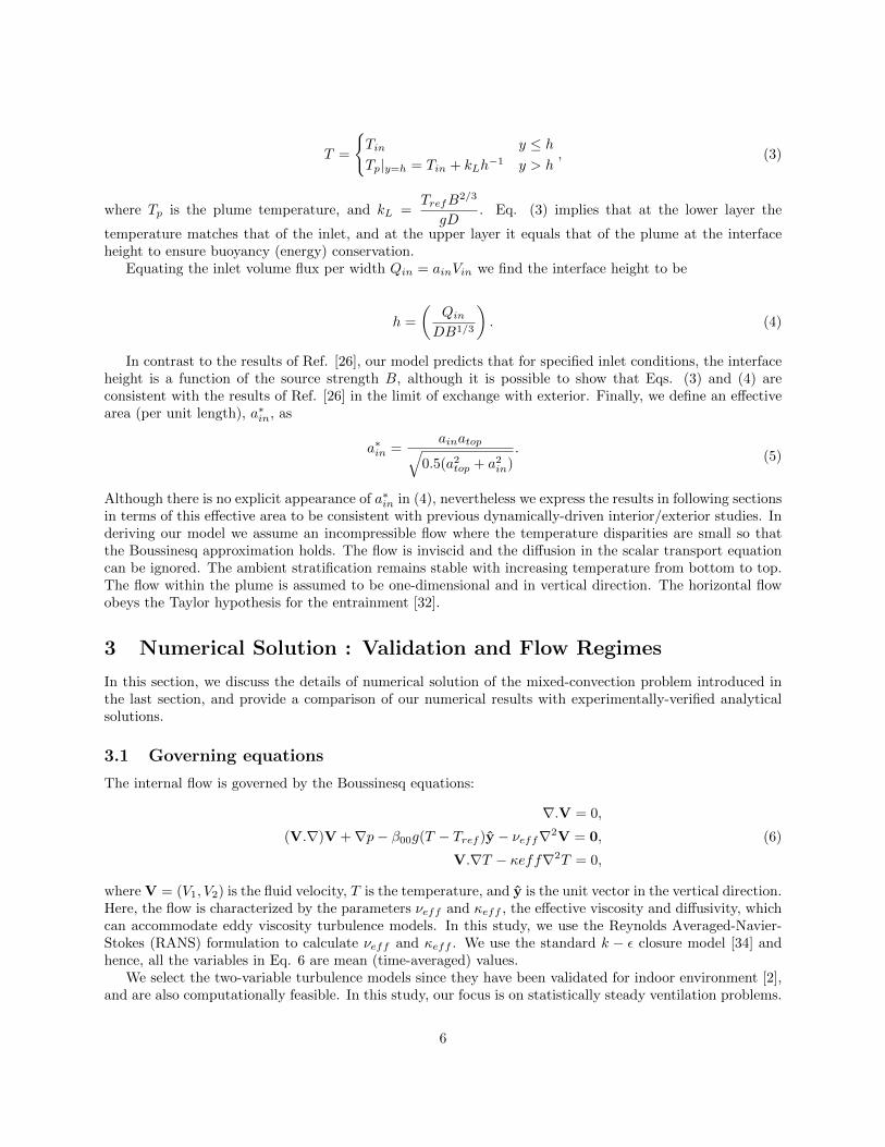
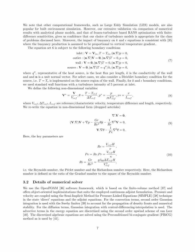
A symmetry plane is introduced at the midplane to save computational cost. Therefore, we only showthe left half of the domain in the results of this section. The height of the interface is measured at the farleft-hand side of the box (away from the plume and the incoming air), and is defined as the height at whichthere is minimal vertical motion, i.e. V2|h ≈ 0. We first vary a∗in to change ζ while keeping Vr constant. Theinterface height as a function of a∗in is plotted in Fig. 2a and the streamlines colored according to scaledtemperature are shown in Fig. 3a-d for different values of a∗in. From Fig. 2a, it can be seen that the interfaceheight varies approximately linearly with respect to a∗in (or Qin); this numerical result is consistent withEq. 4 in the analytical model. For smaller or larger values of a∗in, the non-dimensional interface height,respectively, approaches 0.09 or 0.6 based on our findings, which are the limit of the intermediate regimeand in the following we explore the physical meaning behind such ratios. Therefore deviation from the lineartrend is expected in such cases. There is a small offset (approximately 0.06H) which may be interpretedas a ‘virtual origin’ for the plume consistently with previous studies, (see for example Kaye and Hunt [42]for further discussion). For ζ ≥ 0.6 the interface height is not clearly identified. The temperature andvelocity profile for this case is shown in Fig. 3d. It is seen that by increasing the inlet area, the plumebecomes increasingly detached from the upper layer ambient fluid, and at a critical value of the interfaceheight (Fig. 3d), the horizontal velocity towards the plume becomes negligible. This suggests that the plumetheory foundations, e.g. entrainment hypothesis, self-similarity of velocity profiles, etc. do not hold for thisparameter value, and the plume is now completely isolated from the room fluid, which manifests itself asbypassing of the inlet flow away from the plume and flow directly towards the outlet. This phenomenon isseen to exist for all values of source buoyancy flux, and only depends on ζ. Hence, ζ ≈ 0.6 is the upper limitfor the intermediate regime.

Next, we obtain the range of Vr values corresponding to the intermediate regime. For a given buoyancyflux, we first calculate Vp,max. Then, we vary Vr by altering both ain and Vin while keeping their productQin = ainVin constant. In Fig. 2b, we plot the maximum velocity within the plume as a function of B fortwo values of inlet velocity, Vin. The interface height can be identified for all values of source buoyancy fluxconsidered in Fig. 2b, and the results fall within the intermediate regime. As expected from plume theory[32], Vp,max varies with the power law of 1/3 in both cases, although one case has a two times higher inlet

8

0.005 0.01 0.015 0.020

0.1

0.2

0.3

0.4

0.5

0.6

ain*

h/H

Numerical Simulations Model predictions

(a)

102

103

104

105

10−2

10−1

B

v p,m

ax

Vin

=6 m/s

Vin

=12 m/s

(b)

Figure 2: a) Interface height, ζ, as a function of inlet effective area, a∗in. b) Maximum velocity in the plume, Vp,max as afunction of source buoyancy flux B plotted using log-log axes. Also shown is a line with a slope of 1/3.

0.02-0.01 0.010Theta(a) (b) 0.02-0.01 0.010

Theta

(c) (d)

0.01-0.00 0.0060.0040.0020

Theta(e) (f)

(g) (h)

0.01-0.00 0.0060.0040.0020

Theta

Figure 3: Streamlines colored by scaled temperature for various values of effective area a∗in (a-d) and Vr (e-h). a) a∗in = 0.0066and ζ=0.12, b) a∗in = 0.0158 and ζ=0.5, c) a∗in = 0.0163 and ζ=0.6, d) a∗in = 0.0174 and ζ is not defined. e) Vr = 0.72 andζ=0.52, f) Vr = 1.07 and ζ=0.52, g) Vr = 1.44 and ζ is not defined, and h) Vr = 3.85 and ζ is not defined. The interface heightis indicated by an arrow in each figure.

volume flux. This is further confirmation that for the intermediate regime, our numerical models agree withclassical plume theory. Numerical results are shown in Fig. 3 e-h for the cases where ζ is kept constant andVr is altered. It can be seen that beyond a certain value of Vr, the interface is no longer apparent, and hence,corresponding parameters are not in the intermediate regime. When the vertical velocity of the ambient fluidat the interface becomes comparable to the maximum velocity of the plume, the vertical velocity may not bedownward in the lower layer. The fountain dynamics undergoes a transition and becomes a jet at the inlet.This is consistent with Ref. [43] who observed the same phenomenon, i.e. the transition of a fountain to ajet based on the momentum flux of the injection (although they used a somewhat different Froude number

9

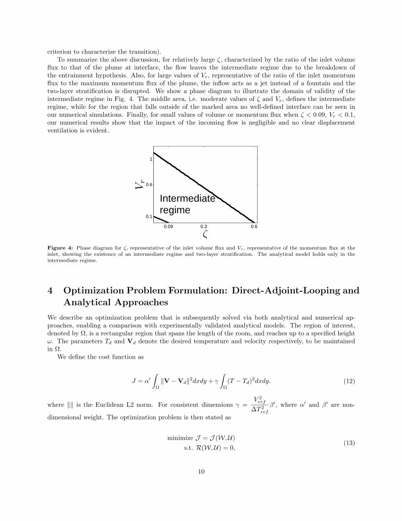
criterion to characterize the transition).To summarize the above discussion, for relatively large ζ, characterized by the ratio of the inlet volume

flux to that of the plume at interface, the flow leaves the intermediate regime due to the breakdown ofthe entrainment hypothesis. Also, for large values of Vr, representative of the ratio of the inlet momentumflux to the maximum momentum flux of the plume, the inflow acts as a jet instead of a fountain and thetwo-layer stratification is disrupted. We show a phase diagram to illustrate the domain of validity of theintermediate regime in Fig. 4. The middle area, i.e. moderate values of ζ and Vr, defines the intermediateregime, while for the region that falls outside of the marked area no well-defined interface can be seen inour numerical simulations. Finally, for small values of volume or momentum flux when ζ < 0.09, Vr < 0.1,our numerical results show that the impact of the incoming flow is negligible and no clear displacementventilation is evident.

0.09 0.3 0.6

0.1

0.6

1

ζ

Vr

Intermediateregime

Figure 4: Phase diagram for ζ, representative of the inlet volume flux and Vr, representative of the momentum flux at theinlet, showing the existence of an intermediate regime and two-layer stratification. The analytical model holds only in theintermediate regime.

4 Optimization Problem Formulation: Direct-Adjoint-Looping andAnalytical Approaches

We describe an optimization problem that is subsequently solved via both analytical and numerical ap-proaches, enabling a comparison with experimentally validated analytical models. The region of interest,denoted by Ω, is a rectangular region that spans the length of the room, and reaches up to a specified heightω. The parameters Td and Vd denote the desired temperature and velocity respectively, to be maintainedin Ω.

We define the cost function as

J = α′∫

Ω

‖V −Vd‖2dxdy + γ

∫Ω

(T − Td)2dxdy. (12)

where ‖‖ is the Euclidean L2 norm. For consistent dimensions γ =V 2ref

∆T 2ref

β′, where α′ and β′ are non-

dimensional weight. The optimization problem is then stated as

minimize J = J (W,U)

s.t. R(W,U) = 0,(13)

10

where W =(V(x, y), p(x, y), T (x, y)

)are the state variables, and U is the set of design variables, i.e.,

U = (Vin, Tin). It should be remembered that the horizontal component of Vin is zero and hence theinlet velocity is unidirectional, and so it is appropriate to express this velocity as a scalar. R denotesthe constraints imposed by the governing equations, corresponding to Boussinesq Eq. (6) in the case ofthe numerical optimization, and the plume Eqs. (3-4) in the case of analytical optimization. Additionalconstraints may also be implemented with no change in the formulation of Eq. (13). We thus have aconstrained optimization problem.

The predicted mean vote (PMV) is commonly used as a measure of thermal comfort in the literature[44]. Such models consider air velocity and temperature as parameters affecting thermal comfort, as well asother parameters, e.g. relative humidity. Here, however, as a proxy for thermal comfort, we measure thediscomfort in the room as the deviation of T from Tcomf , which is defined as the comfortable temperature.We ignore the velocity component in the objective function of thermal comfort, but later we add a constrainton the product of temperature and velocity, as a placeholder for an energy constraint.

4.1 Direct-Adjoint-Looping (DAL) Formulation

We tackle the optimization problem in Eq. (12) by use of the Lagrangian L. We reformulate the optimizationproblem as

minimize L = J + 〈Pᵀ,R〉, (14)

where P = (Va, pa, Ta) is the vector of adjoint variables, and we use the notation 〈f, g〉 =∫D fg dxdy. It

should be noted that we only identify the boundary conditions that (locally) minimize J and there is noclosed-loop control in the current study. The adjoint variables are Lagrange multipliers to enforce the stateEq. (6). To ensure the (at least local) optimality of the solution, we enforce δL = δUL + δWL = 0, whereδG denotes variation of a dependent variable G. We choose the adjoint variables such that δWL = 0. Thesensitivity equations with respect to design variables are then obtained as δL = δUL. This procedure can begeneralized to any number of design variables, and hence contributes to a significant saving in computationaleffort when the number of design variables is large. This idea is at the heart of the adjoint method [15, 16, 17](refer to appendix A for details of our derivation).

By requiring that first order variations with respect to the state variables vanish at optimal solutions,i.e., δWL = 0, we obtain

∇.Va = 0,

−(V.∇)Va +∇Vᵀ.Va +∇pa + T∇Ta + νeff∇2Va + α′(V −Vd) = 0 on Ω,

−∇Vᵀ.Va + (V.∇)Va +∇pa + T∇Ta + νeff∇2Va = 0 on D \ Ω,

V.∇Ta + κeff∇2T − gβ00(T − Tref ) + γ(T − Td) = 0 on Ω,

V.∇Ta + κeff∇2T − gβ00(T − Tref ) = 0 on D \ Ω.

(15)

The adjoint boundary conditions are

inlet : Va = 0, Ta = 0, (n.∇)pa = 0

outlet : VnVa,t + νeff (n.∇)Va,t = 0,

TaVn + κeff (n.∇)Ta = 0,

pa = VnVa,n + V.Va + νeff (n.∇)Va,

wall : Va = 0, (n.∇)Ta = 0, (n.∇)pa = 0,

(16)

where the subscripts n, t denote normal and tangential components, respectively.

11

Now we define non-dimensional variables,

V∗a =Va

Lref, T ∗a =

Ta∇2TrefVrefH

, p∗a =pa

VrefLref, x∗ =

x

Lref. (17)

and the resulting non-dimensional adjoint equations are (dropping asterisks as before):

∇.Va = 0,

−(V.∇)Va +∇VT .Va +∇pa + Ta∇θ −1

Re∇2Va + 2α′(V −Vd) = 0 on Ω,

−(V.∇)Va +∇VT .Va +∇pa + Ta∇θ −1

Re∇2Va = 0 on D \ Ω,

RiVa −V.∇Ta −1

Pe∇2Ta + 2β′(θ − θd) = 0 on Ω,

RiVa.y −V.∇Ta −1

Pe∇2Ta = 0 on D \ Ω.

(18)

Here we have made the choice of using the ‘frozen turbulence’ hypothesis [45]. Hence, we require that(k(x, y), ε(x, y)), which are field variables solved along with

(V(x, y), p(x, y), T (x, y)

)during the forward or

direct simulation, have the same values during the solution of the adjoint equation in the DAL framework.When the number of design variables is small, an assessment of the validity of this assumption can be donefor a given problem by comparing adjoint sensitivities to those computed using a finite-difference method.We relegate this comparison to appendix B. We note that a more comprehensive analysis of the validity ofthe frozen turbulence hypothesis is needed for problems with a higher number of design variables or morecomplicated, possibly time-dependent optimization problems. To validate this hypothesis in a systematicfashion would entail adding adjoint equations for (k, ε) to the set of adjoint equations. A first step in thisdirection was taken in Ref. [46], where a toy-model for a RANS-type closure scheme was considered. In thatstudy, certain energy-exchange mechanisms between the mean-flow and turbulent eddies were found to bepresent only in the adjoint optimization performed without the frozen-turbulence hypothesis.

In the momentum Eq. (18), diffusion is scaled with the inverse of the Reynolds number, or the inverseof the Peclet number for the temperature equation. Hence, by increasing the Reynolds number, the adjointadvection operator, i.e. −(V.∇)Va+∇VT .Va dominates in the velocity equations, and −V.∇Ta dominatesin the temperature equation. Consequently, in numerical implementations, to prevent numerical instabilities,care should be taken in using the correct mesh size, particularly for flows with higher Re.

After computation of the adjoint field we obtain the sensitivity of the cost function with respect to inletvelocity and temperature, i.e. the design variables, as follows

∇VinJ = pa|in −

1

Re(n.∇)Va|in, ∇Tin

J =1

Pe(n.∇)Ta|in. (19)

We illustrate the iterative solution procedure schematically in Fig. 5. Determination of a solution beginswith an initial guess for the design variables (Vin, Tin). The set of ‘direct’ state and adjoint equations aresolved in a loop and the subsequent sensitivity calculation is used to obtain the next guess for the optimaldesign variables. This process is repeated until the convergence criterion for the cost functional is satisfied,i.e. |J n+1 − J n| ≤ ε.

4.2 Analytical optimization for the reduced model

The analytical model derived in Section 2 is now employed to find the optimal inlet conditions, i.e. T oin andV oin. We focus on a local comfort problem, and set α′ = 0 in Eq. (12), with Td = Tcomf . The objectivefunction for thermal comfort problems is then written as

J =

∫Ω

(T − Tcomf )2dxdy.(20)

12

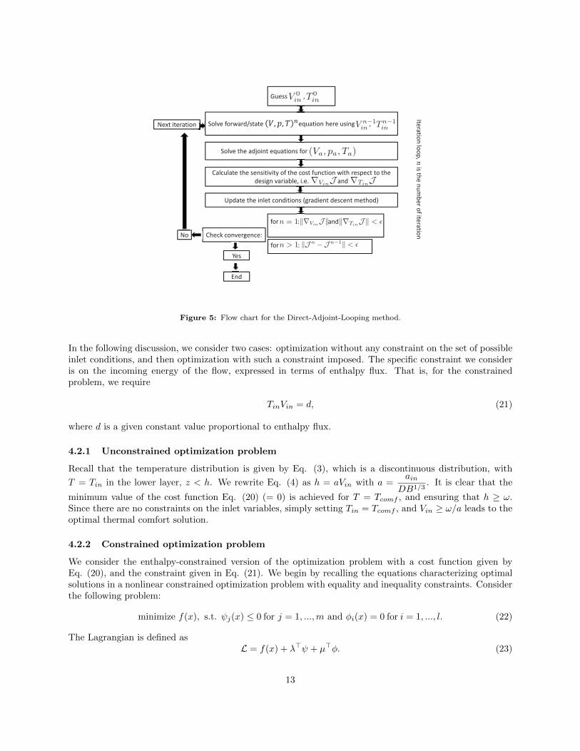
Check convergence:

Update the inlet conditions (gradient descent method)

Itera

tion

loo

p,

is the

nu

mb

er o

f itera

tion

Solve forward/state equation here using ,

Solve the adjoint equations for

Calculate the sensitivity of the cost function with respect to the

design variable, i.e. and

for : and

for :

Guess ,

End

Yes

No

Next iteration

Figure 5: Flow chart for the Direct-Adjoint-Looping method.

In the following discussion, we consider two cases: optimization without any constraint on the set of possibleinlet conditions, and then optimization with such a constraint imposed. The specific constraint we consideris on the incoming energy of the flow, expressed in terms of enthalpy flux. That is, for the constrainedproblem, we require

TinVin = d, (21)

where d is a given constant value proportional to enthalpy flux.

4.2.1 Unconstrained optimization problem

Recall that the temperature distribution is given by Eq. (3), which is a discontinuous distribution, with

T = Tin in the lower layer, z < h. We rewrite Eq. (4) as h = aVin with a =ain

DB1/3. It is clear that the

minimum value of the cost function Eq. (20) (= 0) is achieved for T = Tcomf , and ensuring that h ≥ ω.Since there are no constraints on the inlet variables, simply setting Tin = Tcomf , and Vin ≥ ω/a leads to theoptimal thermal comfort solution.

4.2.2 Constrained optimization problem

We consider the enthalpy-constrained version of the optimization problem with a cost function given byEq. (20), and the constraint given in Eq. (21). We begin by recalling the equations characterizing optimalsolutions in a nonlinear constrained optimization problem with equality and inequality constraints. Considerthe following problem:

minimize f(x), s.t. ψj(x) ≤ 0 for j = 1, ...,m and φi(x) = 0 for i = 1, ..., l. (22)

The Lagrangian is defined asL = f(x) + λ>ψ + µ>φ. (23)

13

Then xo is a local minimum if and only if there exists a unique λo s.t.

∇xL(xo, µo, λo) = 0, (24a)

λo ≥ 0, (24b)

λo>ψ = 0, (24c)

ψ(xo) ≤ 0, (24d)

φ(xo) = 0. (24e)

These five equations characterize a local optimal solution according to Karush-Kuhn-Tucker (KKT) condi-tions [47].

Since the temperature distribution given by Eq. (3) is discontinuous, the optimization problem is solvedin two stages. We first assume ψ = aVin − ω ≤ 0, i.e. the optimal inlet velocity is such that the resultinginterface height is less than or equal to the height of the region of interest. The Lagrangian L for this case is

L = J + λ(aVin − ω) + µ(TinVin − d). (25)

The last term is added due to the enthalpy flux constraint, and µ is the corresponding Lagrange multiplier.Substituting the temperature distribution given in Eq. (3) into Eqs. (25), we obtain

L = (Tin − Tcomf )2ω + 2(Tin − Tcomf )(kLaVin

)(ω − aVin) + (kLaVin

)2(ω − aVin) + λ(aVin − ω) + µ(TinVin − d).

(26)

In the second stage, we apply the KKT condition Eq. (24(a)) i.e. ∇Tin,VinL = 0, to obtain

∂L∂Tin

= 2(Tin − Tcomf )ω + 2(kLaVin

)(ω − aVin) + µVin = 0,

∂L∂Vin

=−2k2

Lω

a2V 3in

− kLaV 2

in

(2ω(Tin − Tcomf )− kL

)+ aλ+ µTin = 0.

(27)

It can be shown that Eq. (27) results in∂L∂Vin

=−k2

L

aV 2in

+aλ+µ(Tin+ kLaVin

) = 0. From the KKT condition

Eq. (24(c)), we obtain either

λo = 0, ψ(xo) ≤ 0, or λo > 0, ψ(xo) = 0.

where xo = Tin, Vin. If λo = 0, we obtain

V oin =ω(kLa

+ d)

− k2L

2(kL + ad)+ kL + Tcomfω

,

T oin = d

− k2L

2(kL + ad)+ kL + Tcomfω

ω(kLa

+ d)

.

(28)

Conversely, if ψ(xo) = 0, we obtain

V oin =ω

a, T oin =

ad

ω, λo =

k2L

ω2+ 2

(ad+ kL)

ω(adω − Tcomf )> 0. (29)

For both these situations, it is still necessary to check that the assumption aV oin ≤ ω holds.

14

We next consider the case when ψ = ω − aVin ≤ 0. For this case, the Lagrangian is

L =

∫ ω

0

(Tin − Tcomf )2dy + λ(ω − aVin) + µ(TinVin − d). (30)

Once again applying the KKT condition Eq. (24(a)), i.e. ∇Tin,VinL = 0, we obtain

∂L∂Tin

= 2(Tin − Tcomf )ω + µVin = 0,∂L∂Vin

= −aλ+ µTin = 0. (31)

Similarly to before, if ψ(xo) = 0, we obtain

V oin =ω

a, T oin =

da

ω, µo = −2a(T oin − Tcomf )λo = −2T oin(T oin − Tcomf ) > 0, (32)

where the last equation holds when Tcomf >da

ω. If λo = 0, we obtain

T oin = Tcomf , Voin =

d

Tcomf. (33)

Depending upon the values of Π1 =da

ωTcomfand Π2 =

a(kLa + d)

− k2L

2(kL + ad)+ kL + Tcomfω

=aV oinω

, the enthalpy-

constrained optimization has one of the three following solutions.

• Case 1 :Π1 ≥ 1, which yields T oin = Tcomf .

• Case 2: Π1 < 1 and Π2 ≤ 1, giving T oin = d

−k2L

2(kL + ad)+ kL + Tcomfω

ω(kLa

+ d)

. This occurs for smaller

values of kL; in the limit kL → 0, T oin = Tcomf .

• Case 3: Π1 < 1 and Π2 > 1, giving T oin =da

ω. This occurs for larger values of kL.

In all of the above cases, the value of the optimal inlet velocity V oin is obtained by using the enthalpy fluxconstraint.

5 Results and Discussion

5.1 Inverse Design

As a first step towards validating the DAL method optimization framework, we use the method to solve aninverse-design problem. We choose arbitrary inlet conditions (T oin, V

oin) and solve the forward problem Eq.

(6) to obtain (V d, T d). We employ the DAL method to optimize the cost function given by Eq. (12). Sincethe optimal solution is known to be (T oin, V

oin), this procedure serves as a method to validate the numerical

optimization framework.For this test case, we use V oin = 12 m/s (vertical velocity only) and T oin = 300 K as the inlet conditions.

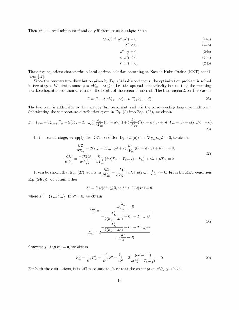
The region of interest height is 40% of that of the room. We start the DAL method from a guess whichis reasonably different compared to the optimal solution, i.e. Tin = 305 K. Fig. 6 shows that after a fewiterations, the optimal inlet conditions are automatically recovered.

15

1 2 3 4 5 6 7 8 9 10300

305

No. iterations

Tin

(k)

1 2 3 4 5 6 7 8 9 100

50

J

Figure 6: Variation of Tin (blue circles) and cost function J (green crosses) with iteration loop number of the DAL methoditeration.

5.2 Optimal Design for Local Thermal Comfort

For unconstrained optimization, the numerical DAL method results in T oin = Tcomf . This is consistentwith the analytical model results presented in Section 4.2.1, with one difference. The sensitivity of thecost function with respect to the inlet velocity, i.e., ∂L

∂V |in is always positive. Hence, the unconstrainedoptimization will lead to a state where the whole room is at Tcomf , a situation which is clearly neither inthe intermediate regime, nor of practical interest.

We now discuss the extension of the DAL method to the more meaningful constrained optimizationproblem discussed in Section 4.2.2. The Lagrangian is written as (also see Appendix A)

L = J+ < Pᵀ,R > +λ(TinVin − d), (34)

The sensitivity with respect to inlet velocity is

∂L∂V|inδVin =

∂J∂V|inδVin+ < P ᵀ,

∂R

∂W > |inδW + λTinδVin, (35)

which yields

∂L∂V|in = −pan + νeff

∂Va

∂n|in + λTinn. (36)

Similarly

∂L∂T|in = −κeff

∂Ta∂n|in + λVin. (37)

From Eqs. (36) and (37), we obtain

λ = −−pa + νeff

∂Va,n∂n

Tin,

(38)

16

and

∂L∂T|in = −νeff

prt

∂Ta∂n|in +

d

T 2in

(− pa + νeff

∂Va,n∂n

). (39)

Eq. (39) computes the true gradient with respect to the inlet temperature, and it is used to improve thenext guess in the constrained DAL method. Note that the corresponding guess for inlet velocity is obtainedfrom the enthalpy flux constraint.

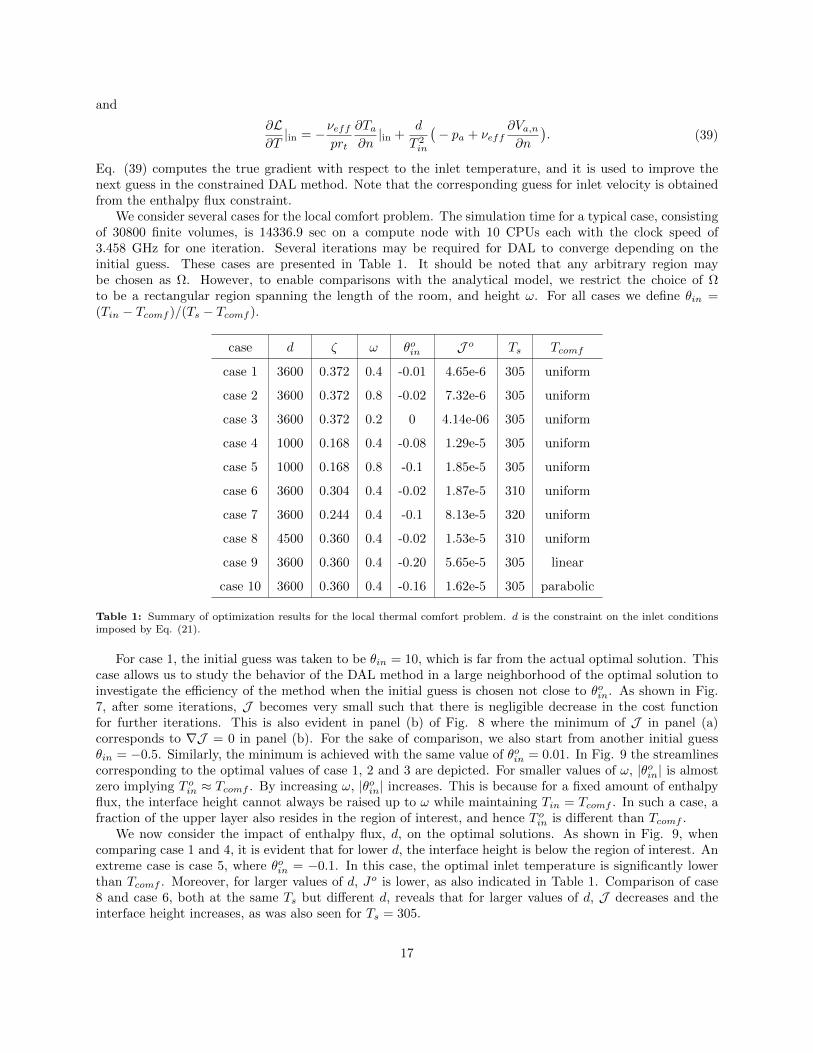
We consider several cases for the local comfort problem. The simulation time for a typical case, consistingof 30800 finite volumes, is 14336.9 sec on a compute node with 10 CPUs each with the clock speed of3.458 GHz for one iteration. Several iterations may be required for DAL to converge depending on theinitial guess. These cases are presented in Table 1. It should be noted that any arbitrary region maybe chosen as Ω. However, to enable comparisons with the analytical model, we restrict the choice of Ωto be a rectangular region spanning the length of the room, and height ω. For all cases we define θin =(Tin − Tcomf )/(Ts − Tcomf ).

case d ζ ω θoin J o Ts Tcomf

case 1 3600 0.372 0.4 -0.01 4.65e-6 305 uniform

case 2 3600 0.372 0.8 -0.02 7.32e-6 305 uniform

case 3 3600 0.372 0.2 0 4.14e-06 305 uniform

case 4 1000 0.168 0.4 -0.08 1.29e-5 305 uniform

case 5 1000 0.168 0.8 -0.1 1.85e-5 305 uniform

case 6 3600 0.304 0.4 -0.02 1.87e-5 310 uniform

case 7 3600 0.244 0.4 -0.1 8.13e-5 320 uniform

case 8 4500 0.360 0.4 -0.02 1.53e-5 310 uniform

case 9 3600 0.360 0.4 -0.20 5.65e-5 305 linear

case 10 3600 0.360 0.4 -0.16 1.62e-5 305 parabolic

Table 1: Summary of optimization results for the local thermal comfort problem. d is the constraint on the inlet conditionsimposed by Eq. (21).

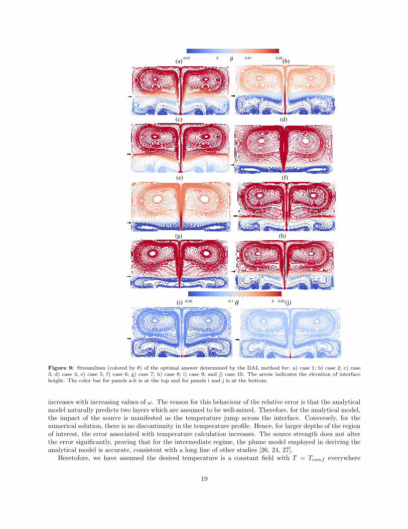
For case 1, the initial guess was taken to be θin = 10, which is far from the actual optimal solution. Thiscase allows us to study the behavior of the DAL method in a large neighborhood of the optimal solution toinvestigate the efficiency of the method when the initial guess is chosen not close to θoin. As shown in Fig.7, after some iterations, J becomes very small such that there is negligible decrease in the cost functionfor further iterations. This is also evident in panel (b) of Fig. 8 where the minimum of J in panel (a)corresponds to ∇J = 0 in panel (b). For the sake of comparison, we also start from another initial guessθin = −0.5. Similarly, the minimum is achieved with the same value of θoin = 0.01. In Fig. 9 the streamlinescorresponding to the optimal values of case 1, 2 and 3 are depicted. For smaller values of ω, |θoin| is almostzero implying T oin ≈ Tcomf . By increasing ω, |θoin| increases. This is because for a fixed amount of enthalpyflux, the interface height cannot always be raised up to ω while maintaining Tin = Tcomf . In such a case, afraction of the upper layer also resides in the region of interest, and hence T oin is different than Tcomf .

We now consider the impact of enthalpy flux, d, on the optimal solutions. As shown in Fig. 9, whencomparing case 1 and 4, it is evident that for lower d, the interface height is below the region of interest. Anextreme case is case 5, where θoin = −0.1. In this case, the optimal inlet temperature is significantly lowerthan Tcomf . Moreover, for larger values of d, Jo is lower, as also indicated in Table 1. Comparison of case8 and case 6, both at the same Ts but different d, reveals that for larger values of d, J decreases and theinterface height increases, as was also seen for Ts = 305.

17

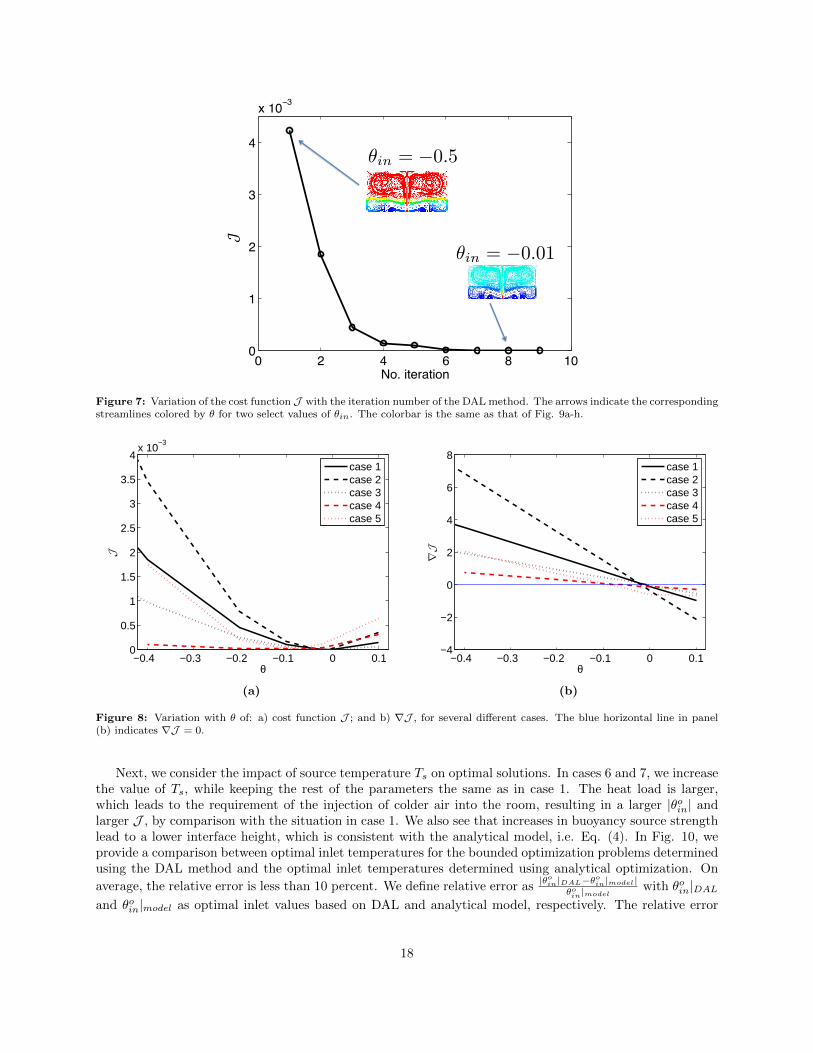
𝒥

Figure 7: Variation of the cost function J with the iteration number of the DAL method. The arrows indicate the correspondingstreamlines colored by θ for two select values of θin. The colorbar is the same as that of Fig. 9a-h.

−0.4 −0.3 −0.2 −0.1 0 0.10

0.5

1

1.5

2

2.5

3

3.5

4x 10

−3

θ

J

case 1case 2case 3case 4case 5

(a)

−0.4 −0.3 −0.2 −0.1 0 0.1−4

−2

0

2

4

6

8

θ

∇J

case 1case 2case 3case 4case 5

(b)

Figure 8: Variation with θ of: a) cost function J ; and b) ∇J , for several different cases. The blue horizontal line in panel(b) indicates ∇J = 0.

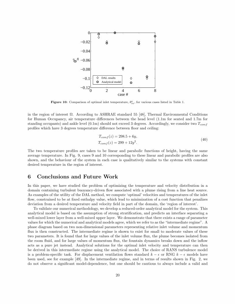
Next, we consider the impact of source temperature Ts on optimal solutions. In cases 6 and 7, we increasethe value of Ts, while keeping the rest of the parameters the same as in case 1. The heat load is larger,which leads to the requirement of the injection of colder air into the room, resulting in a larger |θoin| andlarger J , by comparison with the situation in case 1. We also see that increases in buoyancy source strengthlead to a lower interface height, which is consistent with the analytical model, i.e. Eq. (4). In Fig. 10, weprovide a comparison between optimal inlet temperatures for the bounded optimization problems determinedusing the DAL method and the optimal inlet temperatures determined using analytical optimization. On

average, the relative error is less than 10 percent. We define relative error as|θoin|DAL−θoin|model|

θoin|modelwith θoin|DAL

and θoin|model as optimal inlet values based on DAL and analytical model, respectively. The relative error

18

Theta-0.01 0.010 0.02(a) (b)

(c) (d)

(e) (f)

(g) (h)

0.02-0.20 0-0.1Theta

(i) (j) 0.02-0.20 0-0.1Theta

Figure 9: Streamlines (colored by θ) of the optimal answer determined by the DAL method for: a) case 1; b) case 2; c) case3; d) case 4; e) case 5; f) case 6; g) case 7; h) case 8; i) case 9; and j) case 10. The arrow indicates the elevation of interfaceheight. The color bar for panels a-h is at the top and for panels i and j is at the bottom.

increases with increasing values of ω. The reason for this behaviour of the relative error is that the analyticalmodel naturally predicts two layers which are assumed to be well-mixed. Therefore, for the analytical model,the impact of the source is manifested as the temperature jump across the interface. Conversely, for thenumerical solution, there is no discontinuity in the temperature profile. Hence, for larger depths of the regionof interest, the error associated with temperature calculation increases. The source strength does not alterthe error significantly, proving that for the intermediate regime, the plume model employed in deriving theanalytical model is accurate, consistent with a long line of other studies [26, 24, 27].

Heretofore, we have assumed the desired temperature is a constant field with T = Tcomf everywhere

19

0 2 4 6 8−0.12

−0.1

−0.08

−0.06

−0.04

−0.02

0

case #

θ ino

DAL results

Analytical model

Figure 10: Comparison of optimal inlet temperature, θoin, for various cases listed in Table 1.

in the region of interest Ω. According to ASHRAE standard 55 [48], Thermal Environmental Conditionsfor Human Occupancy, air temperature differences between the head level (1.1m for seated and 1.7m forstanding occupants) and ankle level (0.1m) should not exceed 3 degrees. Accordingly, we consider two Tcomfprofiles which have 3 degrees temperature difference between floor and ceiling:

Tcomf (z) = 298.5 + 6y,

Tcomf (z) = 299 + 12y2.(40)

The two temperature profiles are taken to be linear and parabolic functions of height, having the sameaverage temperature. In Fig. 9, cases 9 and 10 corresponding to these linear and parabolic profiles are alsoshown, and the behaviour of the system in each case is qualitatively similar to the systems with constantdesired temperature in the region of interest.

6 Conclusions and Future Work

In this paper, we have studied the problem of optimizing the temperature and velocity distribution in adomain containing turbulent buoyancy-driven flow associated with a plume rising from a line heat source.As examples of the utility of the DAL method, we compute ‘optimal’ velocities and temperatures of the inletflow, constrained to be at fixed enthalpy value, which lead to minimization of a cost function that penalizesdeviation from a desired temperature and velocity field in part of the domain, the ‘region of interest’.

To validate our numerical methodology, we develop a reduced-order analytical model for the system. Thisanalytical model is based on the assumption of strong stratification, and predicts an interface separating awell-mixed lower layer from a well-mixed upper layer. We demonstrate that there exists a range of parametervalues for which the numerical and analytical models agree, which we refer to as the “intermediate regime”. Aphase diagram based on two non-dimensional parameters representing relative inlet volume and momentumflux is then constructed. The intermediate regime is shown to exist for small to moderate values of thesetwo parameters. It is found that for large values of the inlet volume flux, the plume becomes isolated fromthe room fluid, and for large values of momentum flux, the fountain dynamics breaks down and the inflowacts as a pure jet instead. Analytical solutions for the optimal inlet velocity and temperature can thenbe derived in this intermediate regime using the analytical model. The choice of RANS turbulence modelis a problem-specific task. For displacement ventilation flows standard k − ε or RNG k − ε models havebeen used, see for example [49]. In the intermediate regime, and in terms of results shown in Fig. 2, wedo not observe a significant model-dependence, but one should be cautious to always include a valid and

20

appropriate turbulence model. The DAL method can be extended to any RANS two-variable turbulencemodes in a straightforward manner, should one need to consider a different approach.

An initial validation of the numerical optimization method is done using an inverse-design problem. Weshow that the DAL method recovers the design inlet velocity and temperature exactly. Several cases ofenthalpy-constrained optimization are then studied. If the enthalpy is chosen to be high enough, the optimaltemperature is seen to be approaching the desired temperature in the region of interest, and the interfaceheight is at or above the upper boundary of that region. For a fixed value of inlet enthalpy, increasing theheight of the region of interest results in an optimal solution where part of the upper layer is inside thatregion. We also compute optimal solutions for cases where the desired temperature increases linearly orquadratically with height. In the intermediate regime, it is found that the optimal solutions from numericaland analytical optimization are within 10% of each other.

The test case we consider is the displacement ventilation, due to its vast practical importance [24]. Indisplacement ventilation, the direct supply of ambient cold air and resulting temperature stratification inthe building may be associated with thermal discomfort [50]. For the case where inlet energy/enthalpy isnot constrained, the displacement ventilation may break down, and the stratified two layer room may turninto mixing ventilation [51]. Therefore, we focus on the practically relevant constrained optimization ofdisplacement ventilation. For a given heat load in the room, provided that H is large enough so that theset of parameters are in the intermediate regime, our algorithm optimizes temperature distribution in theoccupied region under the constraint of fixed enthalpy flux of the inlet.

Implementing a correct thermal comfort model requires consideration of several parameters such as airtemperature, velocity, relative humidity, clothing, and even mindset of occupants, which in turn necessitatesconsideration of additional constraints that is beyond the scope of the present manuscript and demands itsown specific research. Of course, various efforts have been made in this direction [52]. However, the conclusionto be drawn from Laftchiev and Nikovski discussion [52] is that different techniques yield different degrees ofthermal satisfaction. Our proposed framework is able to accommodate more complicated cost functions asequations are derived in terms of variations with respect to velocity and temperature of a general, unspecifiedcost function J , i.e. ∂J

∂V ,∂J∂θ , in Appendix A. An important feature of the current modeling is the objective

function can be expressed in terms of field variables and hence, not only more complicated thermal comfortand energy consumption, but also air quality problems can be tackled with a similar approach.

For an initial guess that is far from the optimal solution, numerical challenges may be observed. Ournumerical results show that if the deviation of the initial guess from the optimal solution is significant, a veryrefined mesh is required for convergence of the adjoint equations. We believe that the reason is the sourceterms in Eq. 18 become much larger than other terms, which necessitates a very accurate mesh. However,within a reasonable vicinity of optimal solution, and as is evident from the analytical optimization results,there is no multiplicity. Our knowledge about the physics of the problem considered in this study assists usto start with a guess that does not result in numerical problems.

This work is a first step towards the development of a validated numerical optimization and controlframework for turbulent indoor airflow dynamics. The close agreement of the optimal solutions computedusing the DAL method for this test-case with those obtained from experimentally validated analytical modelsprovides motivation for further development of numerical optimization tools for optimal design of the indoorenvironment. Nevertheless, several challenging problems need to be solved before the methods described inthis work can be applied in realistic settings. For example, there exist several analytical models for transientventilation dynamics, and the various dynamical behaviors are well-understood. The numerical optimizationof transient problems has much higher computational burden than the steady state cases considered here, andare natural candidates for numerical reduced-order modeling, especially in the context of real-time control.Furthermore, we have employed the frozen turbulence assumption in our numerical optimization method.While we confirm the validity of this approach via comparison with finite-difference sensitivity computations,more work needs to be done in order to identify conditions under which this approach breaks down. It isplausible that some optimal solutions to certain classes of indoor airflow optimization problems, e.g. thoseat least related to optimal mixing, may be found only by using the full set of adjoint equations, includingthose corresponding to the turbulence variables such as (k, ε). Of course, this issue is not just confined to

21

indoor airflow. A vast array of practical engineering problems involve turbulent flow, and optimization usingdirect numerical simulation models is not feasible in most cases. The extension of our framework to dealwith these issues will be a topic of future work.

A Derivation of adjoint equations

A popular method to derive optimality conditions is the Lagrangian method [15, 17, 53]. In this approach,a Lagrangian is introduced to PDE-constrained optimization to account for governing equations and otherbounds on design variables. The augmented objective functional, i.e. Lagrangian, is

δL = δJ+ < Pᵀ,∂R

∂W δW > +

∫(λ∂F∂U δU).ndS, (41)

with < . > denoting volume integration and F is any constraint, e.g. the energy of inlet flow, other thanthe governing equations themselves. Here, y is the unit vector in the direction of gravitational acceleration,Pᵀ = (Va, pa, Ta) , Uᵀ = (Vin, θin) and ∂R

∂W and ∂F∂U are Jacobians of the constraints (the Navier-Stokes

equations, the continuity equation and the energy equation) and the objective or cost functional, respectively,with respect to direct variables and input (control) variables; i.e.

∂R

∂W δW =

(δV.∇)V + (V.∇)δV − 1

Re∇2δV − (Ray)δθ +∇δp∇.δV

δV.∇θ + V.∇δθ − 1Pe∇2δθ

. (42)

Using 42, 41 can be rewritten as

δL = δVJ + δpJ + δθJ+ < Va, (δV.∇)V + (V.∇)δV − 1

Re∇2δV − (Ray)δθ +∇δp > +

< pa,∇.δV > + < Ta, δV.∇θ + V.∇δθ − 1

Pe∇2δθ > +

∫(λ∂F∂U δU).ndS.

(43)

For unbounded optimization, F=0 and hence ∂F∂U δU=0. For the optimization constrained by an enthalpy

condition, F = Vinθin, and so

∂F∂U δU =

Vinδθin

θinδVin

. (44)

Each term of (42) can be calculated analytically. Specifically, using vector calculus and integration by parts,appropriate Euler-Lagrange equations can be derived.

δL =< δV,∂J∂V−∇pa − (V.∇)Va + (∇V)ᵀVa −

1

Re∇2Va + Ta∇θ > +

< δp,∇.Va > + < δθ,∂J∂θ−V.∇Ta −

1

Pe∇2Ta + (Riy)Va > +∫

(δV)(pa + Va(V.n) +1

Re∇Va).ndS +

∫(δθ)(Ta(V.n) +

1

Re∇Ta)dS

(45)

To ensure local optimality it is required that δL = 0. From the space integral, the adjoint equations arerecovered as

22

∇.Va = 0,

−(V.∇)Va +∇VT .Va +∇pa + Ta∇θ −1

Re∇2Va +

∂J∂V

= 0,

RiVa.y − V.∇Ta −1

Pe∇2Ta +

∂J∂θ

= 0.

(46)

From surface integrations and after some simplifications [15], we obtain the adjoint boundary conditions:

inlet : Va = 0, Ta = 0, (n.∇)pa = 0,

outlet : VnVa,t +1

Re(n.∇)Va,t = 0,

TaVn +1

Pe(n.∇)Ta = 0,

pa = VnVa,n +1

Re(n.∇)Va,

wall : Va = 0, (n.∇)Ta = 0, (n.∇)pa = 0.

(47)

B Validation of the frozen-turbulence hypothesis for computingadjoint-based sensitivities

We compare the adjoint-based sensitivities, that have been computed using the frozen-turbulence hypothesis,with those computed by a finite-difference (FD) method. Referring to the general first-order forward Eulerapproximation of a derivative, we obtain

∇VinJ |FD =

J (Vin + δVin)− J (Vin − δVin)

2δVin,

∇TinJ |FD =

J (Tin + δTin)− J (Tin − δTin)

2δTin,

∇VinJ |ad =

∫in

(−pa + νeff (n.∇)Va)dA,

∇VinJ |ad =

∫in

(κeff (n.∇)Ta)dA.

(48)

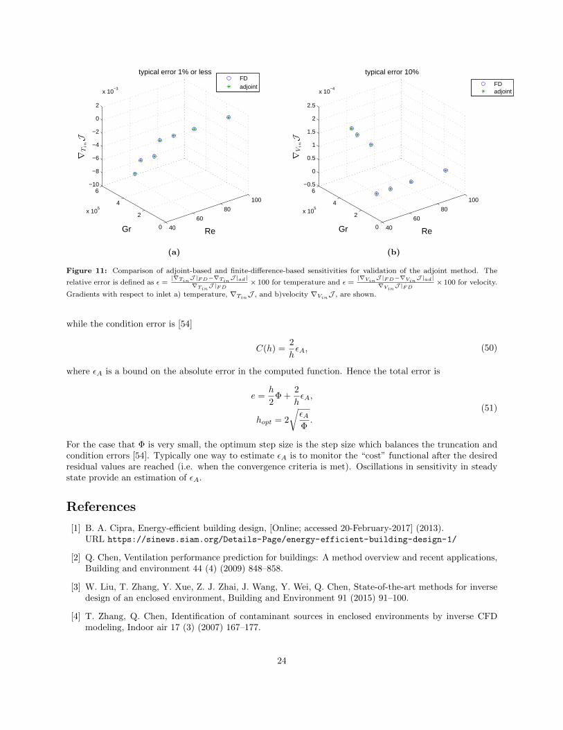
Fig. 11 shows the results of just such a comparison. Overall, the two methods give similar values forsensitivities. This confirms that our numerical framework is robust, and the assumption of frozen-turbulencein our DAL method does not introduce errors in the computation of optimization problem.

The process of choosing an appropriate step size for the finite difference method is non-trivial. Thereare two types of errors in the finite difference approximation: truncation error and condition error. Thetruncation error is the error introduced due to neglecting higher order terms in the Taylor expansion. Thecondition error is associated with numerical noise, and is caused by loss of numerical precision. It may bea result of computer round-off error, or the operation of subtracting large numbers which are very nearlyequal. On reducing step-size, the truncation error decreases while the condition error generally increases.Therefore an estimation of each error is crucial in finite-difference evaluation of sensitivities; there can beeven an optimal step size that can decrease the time and cost of the calculations. The truncation error is

T (h) =h

2f ′′(x),

f ′′(x) ≈ Φ =f(x+ h)− 2f(x) + f(x− h)

h2,

(49)

23

40

60

80

100

0

2

4

6

x 105

−10

−8

−6

−4

−2

0

2

x 10−3

Re

typical error 1% or less

Gr

∇TinJ

FDadjoint

(a)

40

60

80

100

0

2

4

6

x 105

−0.5

0

0.5

1

1.5

2

2.5

x 10−4

Re

typical error 10%

Gr

∇VinJ

FDadjoint

(b)

Figure 11: Comparison of adjoint-based and finite-difference-based sensitivities for validation of the adjoint method. The

relative error is defined as ε =|∇Tin

J |FD−∇TinJ |ad|

∇TinJ |FD

× 100 for temperature and ε =|∇Vin

J |FD−∇VinJ |ad|

∇VinJ |FD

× 100 for velocity.

Gradients with respect to inlet a) temperature, ∇TinJ , and b)velocity ∇Vin

J , are shown.

while the condition error is [54]

C(h) =2

hεA, (50)

where εA is a bound on the absolute error in the computed function. Hence the total error is

e =h

2Φ +

2

hεA,

hopt = 2

√εAΦ.

(51)

For the case that Φ is very small, the optimum step size is the step size which balances the truncation andcondition errors [54]. Typically one way to estimate εA is to monitor the “cost” functional after the desiredresidual values are reached (i.e. when the convergence criteria is met). Oscillations in sensitivity in steadystate provide an estimation of εA.

References

[1] B. A. Cipra, Energy-efficient building design, [Online; accessed 20-February-2017] (2013).URL https://sinews.siam.org/Details-Page/energy-efficient-building-design-1/

[2] Q. Chen, Ventilation performance prediction for buildings: A method overview and recent applications,Building and environment 44 (4) (2009) 848–858.

[3] W. Liu, T. Zhang, Y. Xue, Z. J. Zhai, J. Wang, Y. Wei, Q. Chen, State-of-the-art methods for inversedesign of an enclosed environment, Building and Environment 91 (2015) 91–100.

[4] T. Zhang, Q. Chen, Identification of contaminant sources in enclosed environments by inverse CFDmodeling, Indoor air 17 (3) (2007) 167–177.

24

[5] T. Zhang, Q. Chen, Identification of contaminant sources in enclosed spaces by a single sensor, Indoorair 17 (6) (2007) 439–449.

[6] T. T. Zhang, S. Yin, S. Wang, An inverse method based on CFD to quantify the temporal release rateof a continuously released pollutant source, Atmospheric environment 77 (2013) 62–77.

[7] W. Liu, M. Jin, C. Chen, Q. Chen, Optimization of air supply location, size, and parameters in en-closed environments using a computational fluid dynamics-based adjoint method, Journal of BuildingPerformance Simulation 9 (2) (2016) 149–161.

[8] A. Sempey, C. Inard, C. Ghiaus, C. Allery, Fast simulation of temperature distribution in air conditionedrooms by using proper orthogonal decomposition, Building and Environment 44 (2) (2009) 280–289.

[9] B. Kramer, P. Grover, P. Boufounos, M. Benosman, S. Nabi, Sparse sensing and DMD based identifi-cation of flow regimes and bifurcations in complex flows, arXiv preprint arXiv:1510.02831.

[10] Y. Xue, Z. J. Zhai, Q. Chen, Inverse prediction and optimization of flow control conditions for confinedspaces using a CFD-based genetic algorithm, Building and Environment 64 (2013) 77–84.

[11] C. W. Rowley, S. T. Dawson, Model reduction for flow analysis and control, Annual Review of FluidMechanics 49 (2017) 387–417.

[12] W. K. Anderson, V. Venkatakrishnan, Aerodynamic design optimization on unstructured grids with acontinuous adjoint formulation, Computers & Fluids 28 (4) (1999) 443–480.

[13] F. Muyl, L. Dumas, V. Herbert, Hybrid method for aerodynamic shape optimization in automotiveindustry, Computers & Fluids 33 (5) (2004) 849–858.

[14] R. Lanzafame, M. Messina, Fluid dynamics wind turbine design: Critical analysis, optimization andapplication of bem theory, Renewable energy 32 (14) (2007) 2291–2305.

[15] C. Othmer, A continuous adjoint formulation for the computation of topological and surface sensitivitiesof ducted flows, International Journal for Numerical Methods in Fluids 58 (8) (2008) 861–877.

[16] R. Kerswell, C. Pringle, A. Willis, An optimization approach for analysing nonlinear stability withtransition to turbulence in fluids as an exemplar, Reports on Progress in Physics 77 (8) (2014) 085901.

[17] D. Foures, C. Caulfield, P. J. Schmid, Optimal mixing in two-dimensional plane poiseuille flow at finitepeclet number, Journal of Fluid Mechanics 748 (2014) 241–277.

[18] S. Rabin, C. Caulfield, R. Kerswell, Designing a more nonlinearly stable laminar flow via boundarymanipulation, Journal of Fluid Mechanics 738 (2014) R1.

[19] J. A. Burns, J. Borggaard, E. Cliff, L. Zietsman, An optimal control approach to sensor / actuatorplacement for optimal control of high performance buildings, International High Performance BuildingsConference at Purdue, July 16-19, 2012.

[20] X. Zhao, W. Liu, S. Liu, Y. Zou, Q. Chen, Inverse design of an indoor environment using a CFD-based adjoint method with the adaptive step size for adjusting the design parameters, Numerical HeatTransfer, Part A: Applications 71 (7) (2017) 707–720.

[21] J. Borggaard, J. A. Burns, A. Surana, L. Zietsman, Control, estimation and optimization of energyefficient buildings, in: American Control Conference, 2009. ACC’09., IEEE, 2009, pp. 837–841.

[22] W. Liu, Q. Chen, Optimal air distribution design in enclosed spaces using an adjoint method, InverseProblems in Science and Engineering 23 (5) (2015) 760–779.

25

[23] E. Turgeon, D. Pelletier, J. Borggaard, A continuous sensitivity equation approach to optimal design inmixed convection, Numerical Heat Transfer: Part A: Applications 38 (8) (2000) 869–885.

[24] P. F. Linden, The fluid mechanics of natural ventilation, Annual review of fluid mechanics 31 (1) (1999)201–238.

[25] W. Baines, J. Turner, Turbulent buoyant convection from a source in a confined region, Journal of Fluidmechanics 37 (01) (1969) 51–80.

[26] P. Linden, G. Lane-Serff, D. Smeed, Emptying filling boxes: the fluid mechanics of natural ventilation,Journal of Fluid Mechanics 212 (1990) 309–335.

[27] N. Kaye, G. Hunt, Time-dependent flows in an emptying filling box, Journal of Fluid Mechanics 520(2004) 135–156.

[28] D. Bolster, C. Caulfield, Transients in natural ventilationa time-periodically-varying source, BuildingServices Engineering Research and Technology 29 (2) (2008) 119–135.

[29] D. Bower, C. Caulfield, S. Fitzgerald, A. Woods, Transient ventilation dynamics following a change instrength of a point source of heat, Journal of Fluid Mechanics 614 (2008) 15.

[30] S. Nabi, M. Flynn, The hydraulics of exchange flow between adjacent confined building zones, Buildingand Environment 59 (2013) 76–90.

[31] J. Craske, M. van Reeuwijk, Generalised unsteady plume theory, Journal of Fluid Mechanics 792 (2016)1013–1052.

[32] B. Morton, G. Taylor, J. Turner, Turbulent gravitational convection from maintained and instantaneoussources, in: Proceedings of the Royal Society of London A: Mathematical, Physical and EngineeringSciences, Vol. 234, The Royal Society, 1956, pp. 1–23.

[33] S. Nabi, M. Flynn, Buoyancy-driven exchange flow between two adjacent building zones connected withtop and bottom vents, Building and Environment 92 (2015) 278–291.

[34] B. Mohammadi, O. Pironneau, Analysis of the k-epsilon turbulence model (1993) France: EditionsMASSON.

[35] R. Henkes, F. Van Der Vlugt, C. Hoogendoorn, Natural-convection flow in a square cavity calculatedwith low-reynolds-number turbulence models, International Journal of Heat and Mass Transfer 34 (2)(1991) 377–388.

[36] Openfoam - the open source computational fluid dynamics (cfd) toolbox (Dec. 2016).URL http://openfoam.com

[37] H. G. Weller, G. Tabor, H. Jasak, C. Fureby, A tensorial approach to computational continuum me-chanics using object-oriented techniques, Computers in physics 12 (6) (1998) 620–631.

[38] S. V. Patankar, D. B. Spalding, A calculation procedure for heat, mass and momentum transfer inthree-dimensional parabolic flows, International journal of heat and mass transfer 15 (10) (1972) 1787–1806.

[39] P. K. Sweby, High resolution schemes using flux limiters for hyperbolic conservation laws, SIAM journalon numerical analysis 21 (5) (1984) 995–1011.

[40] B. Van Leer, Towards the ultimate conservative difference scheme. ii. monotonicity and conservationcombined in a second-order scheme, Journal of computational physics 14 (4) (1974) 361–370.

[41] J. H. Ferziger, M. Peric, A. Leonard, Computational methods for fluid dynamics (1997).

26

[42] N. Kaye, G. Hunt, The effect of floor heat source area on the induced airflow in a room, Building andEnvironment 45 (4) (2010) 839–847.

[43] G. Hunt, H. Burridge, Fountains in industry and nature, Annual Review of Fluid Mechanics 47 (2015)195–220.

[44] P. O. Fanger, et al., Thermal comfort. analysis and applications in environmental engineering., Thermalcomfort. Analysis and applications in environmental engineering.

[45] E. Papoutsis-Kiachagias, K. Giannakoglou, Continuous adjoint methods for turbulent flows, appliedto shape and topology optimization: industrial applications, Archives of Computational Methods inEngineering 23 (2) (2016) 255–299.

[46] D. Foures, C. Caulfield, P. Schmid, Variational framework for flow optimization using seminorm con-straints, Physical Review E 86 (2) (2012) 026306.

[47] S. Boyd, L. Vandenberghe, Convex optimization, Cambridge university press, 2004.

[48] ASHRAE Standard 55-1992, Thermal environmental conditions for human occupancy, 1992.

[49] N. Kaye, Y. Ji, M. Cook, Numerical simulation of transient flow development in a naturally ventilatedroom, Building and Environment 44 (5) (2009) 889–897.

[50] A. Novoselac, J. Srebric, A critical review on the performance and design of combined cooled ceilingand displacement ventilation systems, Energy and buildings 34 (5) (2002) 497–509.

[51] D. L. Loveday, K. C. Parsons, A. H. Taki, S. G. Hodder, et al., Designing for thermal comfort incombined chilled ceiling/displacement ventilation environments/discussion, ASHRAE transactions 104(1998) 901.

[52] E. Laftchiev, D. Nikovski, An iot system to estimate personal thermal comfort, in: Internet of Things(WF-IoT), 2016 IEEE 3rd World Forum on, IEEE, 2016, pp. 672–677.

[53] F. Troltzsch, Optimal control of partial differential equations, volume 112 of graduate studies in math-ematics, American Mathematical Society, Providence, RI.

[54] J. Iott, R. T. Haftka, H. M. Adelman, Selecting step sizes in sensitivity analysis by finite differences,NASA Technical Memorandum, 1985.

27