Adjoint-based optimization of unsteady turbulent flows:

Recent advances and current challenges

(Presented at NIA CFD Seminar )

Boris Diskin

Research Fellow, NIA

April 16, 2013

The Weizmann 2013 Workshop on Multilevel

Computational Methods and Optimization

• This a meeting in honor of Prof. Achi Brandt

• It is a unique forum of experts in multiscale computations

• My talk is probably the only one there that is not directly

focused on a multigrid/multiscale method

• My pitch is to review a cutting-edge method for really large-

scale aerodynamic computations and identify areas that can

benefit from recent multiscale ideas

• The cutting-edge computations of my choice is the adjoint-

based methodology for optimization of unsteady turbulent

flows on dynamic overset grids

• I am not presenting new results, rather reviewing recent

publications

Outline of the talk

• Adjoint-based optimization of unsteady flows

o Overview of the methodology

o Derivation of time-dependent adjoint equations

o Complex-variable verification of sensitivities

o Example: Constrained optimization of a helicopter flow

• Challenges:

o I/O of large amount of data (addressed by HPC)

o Convergence acceleration (addressed by HPC, partially by

multigrid, more improvement needed)

o Possible instability for chaotic flows (help wanted)

o Finding global optimum (help wanted)

Adjoint-Based Optimization of Unsteady

Flows

Overview

• Optimization problems arise in many unsteady aerodynamic applications

including optimal design of helicopters, turbomachinery blades, biologically

inspired UAV, wind-energy configurations, flow control, etc.

• Optimization approach is gradient based, i.e., gradient (sensitivity) of the

target functional is computed wrt all design parameters and optimization

packages such as PORT, NPSOL are used to update design parameters.

• The adjoint methodology is attractive for optimization problems with many

design variables, yet relatively few constraints. An adjoint-based sensitivity

analysis is performed at a cost comparable to a flow solution and

independent of the number of design variables.

• Discrete adjoint is attractive and viable approach for complex large-scale

optimization problems: consistent, rigorous, verifiably accurate

sensitivities, grid sensitivities, potentially automated (with automatic

differentiation), proven to work for large-scale aerodynamic optimization.

Recent references for Time-Dependent

Adjoint Methodology

• Yamaleev N. K., Diskin B., and Nielsen E. J., “Adjoint-Based Methodology

for Time-Dependent Optimization,” AIAA-2008-5857

• Nielsen E. J., Diskin B., and Yamaleev N. K., “Discrete adjoint-based

design optimization of unsteady turbulent flows on dynamic unstructured

grids,” AIAA Journal (2010), 48(6), pp. 1195-1206

• Nielsen E. J. and Diskin B., “Discrete Adjoint-Based Design Optimization

of Unsteady Turbulent Flows on Dynamic Overset Unstructured Grids,”

AIAA-2012-0554

Adjoint-Based Aerodynamic Design

Capabilities in FUN3D (NASA Langley)

• Steady-state adjoint research initiated – 1994

• Fully consistent RANS design capability – 1997

• Verification with complex variables – 1998

• Parallelization – 1999

• Discretely consistent iterations – 2001

• Grid adjoint – 2003

• Complex-variable sensitivity for thermo-chemical

non-equilibrium flows – 2004

• URANS design capability for dynamic grids – 2009

• Optimized I/O for massively parallel architectures - 2010

• Extension to overset grids – 2012

Unsteady Adjoint-Based Design Capabilities on

Dynamic Overset Unstructured Grids

• Extension to dynamic overset grids

opens up many new applications for optimization,

especially those involving large relative motions

- Rotorcraft

- Store/stage-separation problems

- Wind energy devices

- Biologically-inspired configurations

- Turbomachinery

• Many other exciting opportunities

- Error estimation

- Rigorous mesh adaptation

- Uncertainty quantification

Derivation of the Time-Dependent Adjoint

Equations

Flow Equations on Dynamic Grids

Subject to Time-Dependent Reynolds-Averaged Navier-Stokes Equations

Geometric Conservation

Law (GCL):

• GCL is added to preserve constant solution on dynamic grids

• Special interpolation equations for fringe, hole, and orphan points on overset grids are not shown

• 1st order temporal scheme is shown for simplicity, higher-order schemes are used in actual computations

- vector of spatial residuals, - computational grid - initial conditions

- control volume - mesh velocities, - outward unit normal

tfFFf

ba

N

Nn

nnn

),,();(min objobj DXQD

D DD design variables

Grid Equations

( , ) 0n G X DGeneral form:

0 0( , , )n n n n n G X X D X XR

Grids Undergoing Rigid Motion

• Multiple transformations telescope via matrix multiplication (e.g., parent-child body motion)

0( , )n n n n

surf G X D X XK

Deforming Grids

linear elasticity matrix K

• Mesh assumed to obey linear elasticity relations of solid mechanics

• Surface mesh may be further specified according to rigid motion relation

where

matrix of 3x3 blocks specifying rotations

vector of 3x1 blocks specifying translations

R

where

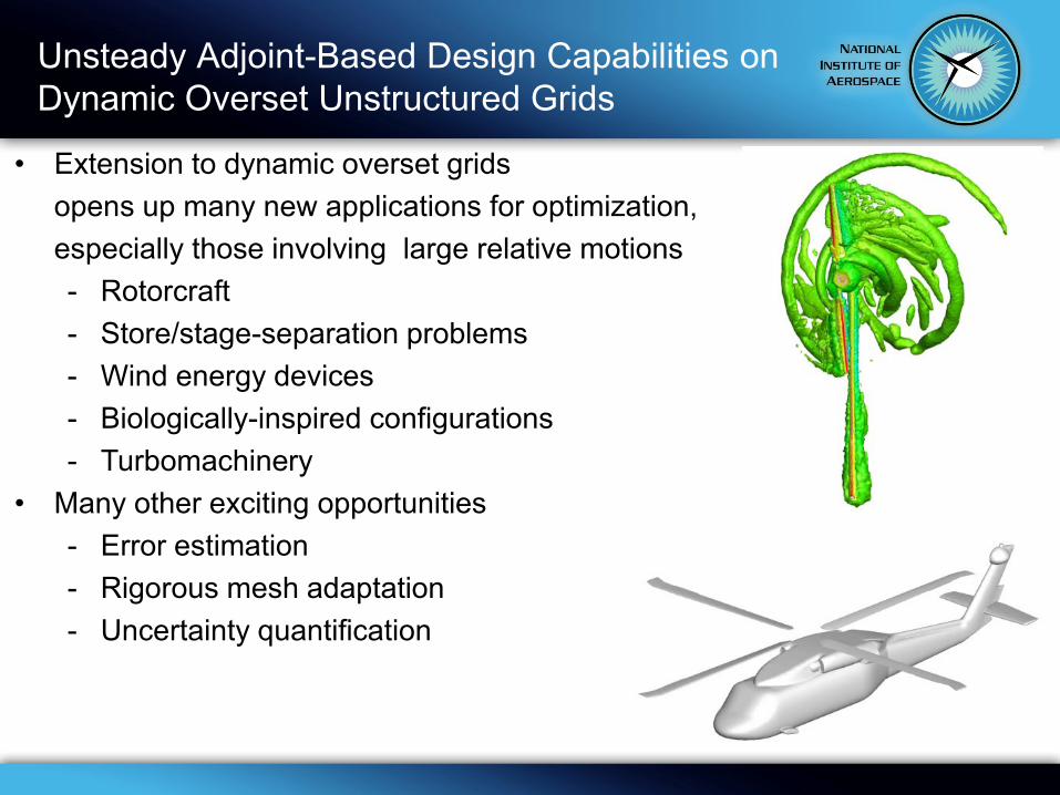
Lagrangian

12

• Overset interpolation equations are omitted for simplicity

• Differentiate wrt D, equate the coefficients of Qn/D and

Xn/D to zero

11

1 1

( , , , , )n nN N

Tn n n n n n

f g f GCL

n n

L f t tt

Q Q

D Q X Λ Λ Λ R QV R

0 0 0 0

1

NT T T

n n in

g f g

n

t f t t

Λ G Λ R Λ G

Objective Function Flow Equations

Grid

Equations Initial Conditions

f Λ g Λ Grid adjoin f Objective function Flow adjoint

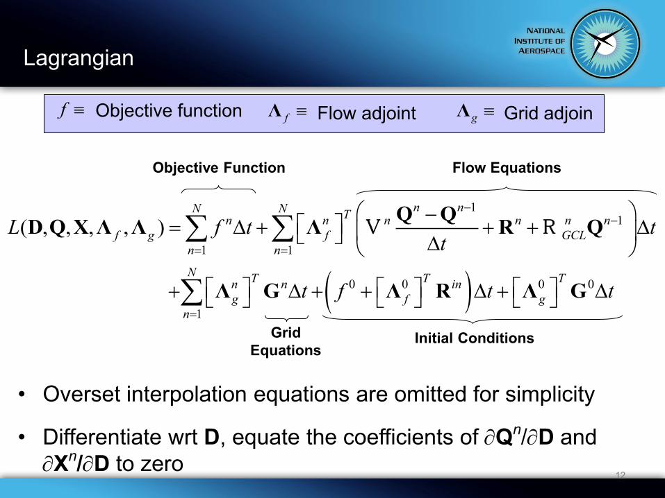
Time-Dependent Adjoint Equations

13

• Dependencies on all time levels in stencil must be linearized

• Traditional steady terms shown in red

1 1 1 11T T

n nnn n n n n n

f f Gf L f nCn

f

t

Λ

QΛ Λ

RΛ

QV V R

01 1 0 1 1

0 0

1T T

in

f f GCL f

f

t

RΛ Λ Λ

Q QV R

Flow

Adjoint

Equations

1 n N

0n

1 11

0

TTn kn n

n n k

T Tn n kn n kg fn n n

GCLfn n

k

f

t

Q Q

ΛG R

Λ ΛX

QXX XX

RV

10 0 10 0 0 1

0 0 0 0 0 01

TT T T Tn inN

n GCLg g f f

n

f

G G R RΛ Λ Λ Q Λ

X X X X X X

R

1 n N Grid

Adjoint

Equations 0n

0 01 0 0

1

n n nT

n inN T TnGCL

f gn

Tn nf g

fLt

d

dt

f

R G

Q Λ ΛD

R GΛ Λ

D D DD D D D

R

Sensitivity Equation

General Unsteady Implementation

• Adjoint solution is initiated at final time level N and

marched in reverse physical time: flow solution Qn at all

time levels must be available during reverse integration

• The approach is to store Qn to disk for all n; also store Xn

and Xn/t for dynamic mesh cases (total of 12

variables/grid point)

– Storage cost can easily yield disk requirement of O(TB)

• Infrastructure required to simultaneously manage/shuffle

data from as many as 7 time levels: current + 3 forward + 3

reverse

Complex-Variable Verification

Verification Using Complex Variables

2( ) ( )( ) ( )

2

f x h f x hf x O h

h

2 3 4

( ) ( ) ( ) ( ) ( ) ( )2 6 24

ivh ih hf x ih f x ihf x f x f x f x

Traditional Central Difference:

Complex Variables (Lyness & Moler, 1966):

Subtractive Cancellation Error

2Im[ ( )]( ) ( )

f x ihf x O h

h

• True second order accuracy: discretely consistent

• Complex-valued FUN3D source code generated automatically via scripting procedure

• h=10-50 for all complex results

• All equation sets converged to machine accuracy

Verification of Implementation Problem Definition

• Fully turbulent flow: M∞=0.1, a=2º, Re=1M, m=0.12

• Composite grid consists of six component grids

• All verification cases run on 360 cores

Component Topology Motion Motion Ancestry

Domain Hex (Cartesian) Inertial Static Great-grandparent

Fuselage Prz/pyr/tet Rotation, translation Rigid Grandparent

Blades Tet Azimuthal rotation Rigid Parent

Blades - 1º vertical oscillatory

rotation about hub Deforming Child

Total Composite

Grid

1,033,243 nodes

3,190,160 elements

Hex/prz/pyr/tet

- Deforming Four generations

Verification of Implementation

After 5 Physical Time Steps

Design Variable BDF1 BDF2 BDF2opt BDF3

Angle of Attack 0.032387388401060

0.032387388401060

0.032390834852470

0.032390834852468

0.032382969025224

0.032382969025223

0.032374960728472

0.032374960728471

Rot Rate

Blade 1 0.049010917009587

0.049010917009599

0.049303058989982

0.049303058989996

0.049392787479850

0.049392787479863

0.049505103043920

0.049505103043932

Shape

Blade 2 -0.004741396075215

-0.004741396075140

-0.005822463933444

-0.005822463933378

-0.005891431208194

-0.005891431208081

-0.006004976330078

-0.006004976329965

Flap Freq

Blade 3 -0.117898939551988

-0.117898939551986

-0.117819415724222

-0.117819415724217

-0.117766926835991

-0.117766926835985

-0.117703857525237

-0.117703857525232

Rot Rate

Fuselage 0.069017024693610

0.069017024693502

0.064234646041659

0.064234646041451

0.064468559766846

0.064468559764283

0.064688175664501

0.064688175664242

Trans Rate

Fuselage -0.002337944913071

-0.002337944913072

-0.002888267191799

-0.002888267191802

-0.002909479741304

-0.002909479741305

-0.002940703514842

-0.002940703514857

Shape

Fuselage -0.000035249806854

-0.000035249806854

-0.000039222298162

-0.000039222298162

-0.000039485944155

-0.000039485944155

-0.000039831885096

-0.000039831885096

LC D

Large-Scale Optimization

• Composite grid consists of 9,262,941 nodes / 54,642,499 tetrahedra

• Compressible RANS: Mtip=0.64, Retip=7.3M, m=0.37, a=0.0º

• Time step corresponds to 1º of rotor rotation

• Blade pitch has a motion governed by collective and cyclic control inputs:

• Baseline value of all control inputs is zero

UH-60A Blackhawk Helicopter Overview

1 1cos sinc c s

Blade

pitch Collective Lateral cyclic Longitudinal cyclic

• Baseline conditions yield untrimmed flight with =0.023 over second rev

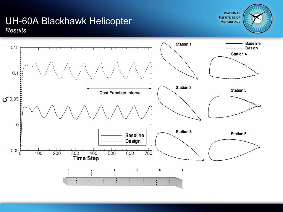
• Objective is to maximize while satisfying trim constraints over second rev:

• Separate adjoint solutions required for all three functions

UH-60A Blackhawk Helicopter Problem Definition

LC

LC

2720

361

1min 2.0

360

n

L

n

f C t

720

1

361

10

360 x

n

M

n

g C t

720

2

361

10

360 y

n

M

n

g C t

such that

Blade shape design variable locations

67 design variables include 64

thickness and camber variables across

the blade planform, plus collective and

cyclic control inputs up to ±7º

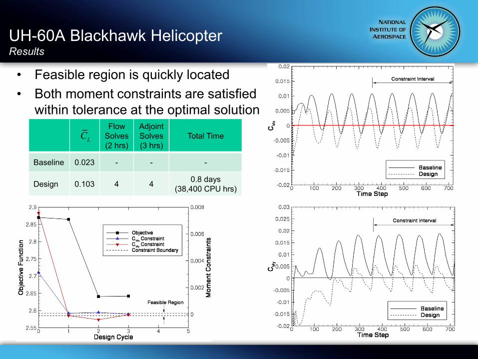
UH-60A Blackhawk Helicopter Results

• Feasible region is quickly located

• Both moment constraints are satisfied

within tolerance at the optimal solution Flow

Solves

(2 hrs)

Adjoint

Solves

(3 hrs)

Total Time

Baseline 0.023 - - -

Design 0.103 4 4 0.8 days

(38,400 CPU hrs)

LC

UH-60A Blackhawk Helicopter Results

Interpretation of Adjoint Solutions

• Adjoint shows sensitivity of objective function to local disturbances in space and time

• Solution can be used for sensitivity analysis, rigorous error estimation and mesh adaptation

– Traditional feature-based techniques do not identify such regions

Animations shown in reverse physical time

Helicopter Wind Turbine

Other Applications of Time-Dependent Adjoint Method

• Formal treatment of MDO problems • Sonic boom

– CFD-ground propagation

• Rotorcraft

– CFD-structures-trim-rigid dynamics

• Acoustics

– CFD-noise

• Laminar flow control

– CFD-transition

• Time-dependent mesh adaptation, error estimation, and uncertainty quantification

Challenge: Large Memory Requirements

I/O of Large Amounts of Data

• For large-scale optimization of unsteady problems, massively parallel computing must be used as efficiently as possible

• Parallel efficiency is complicated by the need for frequent disk I/O involving large amounts of data

– Flow solver must write solution to disk at each time step

– Adjoint solver must read solution from disk at each time step

• This disk I/O can be prohibitively expensive if implemented in a naïve fashion. Sequential I/O is not acceptable.

• I/O is scalable and efficient in high-performance computing (HPC) environment

E. J. Nielsen and W.T. Jones, “Integrated Design of an Active Flow Control System Using a Time-Dependent Adjoint Method.” Mathematical Modeling of Natural Phenomena, Vol. 6, No. 3, 2011, pp. 141-165

I/O of Large Amounts of Data:

HPC Environment

• O(10^3) processors, O(10^5) grid nodes per processor

• Lustre-based parallel scalable direct-access file system – Each processor writes to (reads from) its own direct-access file

– File pointer is placed precisely at the record of interest and I/O may proceed immediately

– Direct-access method is ~2 orders of magnitude faster than traditional sequential-access approach

– Sufficient disk space (petabytes of storage)

• Asynchronous I/O – I/O data is buffered, while execution continues

– “Hides” the cost of doing I/O behind the FLOPs

– Avoid altering the relevant data before the actual I/O has occurred

• In the current HPC environment, I/O of large amounts of

data is NOT a bottleneck

Challenge: Convergence Acceleration

Multigrid

• CFD solutions may require many months of high-performance

computing

• Multigrid is pioneered and advocated by Achi Brandt as the

most powerful method for convergence acceleration

• Our focus is on geometrical nonlinear multigrid for turbulent

flows on general unstructured grids (UG)

• Traditional “nested” multigrid is not well suited for UG

applications.

• Agglomeration multigrid (AgMG) is better suited.

Recent AgMG Advancements with Hiro Nishikawa (NIA) and Jim Thomas (NASA LaRC)

• Focus on methods that converge to machine-zero residuals

• Developed and applied unique idealized multigrid analysis

tools suitable for UG (2004, 2005, 2010)

– Idealized relaxation (tests coarse grid correction)

– Idealized coarse grid (tests relaxation)

• Extended hierarchical multigrid method (1999) to UG

– Developed AgMG method preserving features of geometry (2010)

– Critically assessed and improved AgMG for diffusion (2010)

– Applied AgMG to complex inviscid/laminar/turbulent flows (2010)

– Extended AgMG for parallel computations (2011)

– Improved robustness and efficiency of relaxation (2013)

• Implemented AgMG in FUN3D (NASA), collaboration on

implementation in BCFD (Boeing), TAU (DLR), JAXA

Parallel AgMG for Turbulent Flows (2011)

CFL = 200

60K nodes/processor

Transonic Turbulent Flow,

DPW-4 wing-body-tail configuration

Single Grid

Multigrid

CFL = 200, 10M nodes

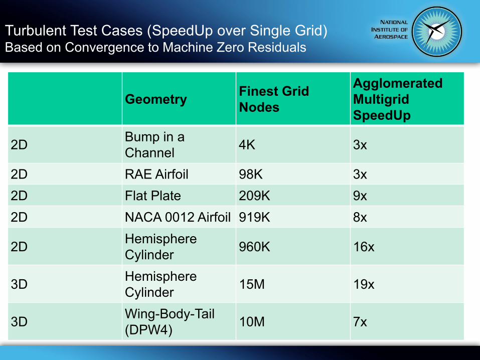
Turbulent Test Cases (SpeedUp over Single Grid) Based on Convergence to Machine Zero Residuals

Geometry Finest Grid

Nodes

Agglomerated

Multigrid

SpeedUp

2D Bump in a

Channel 4K 3x

2D RAE Airfoil 98K 3x

2D Flat Plate 209K 9x

2D NACA 0012 Airfoil 919K 8x

2D Hemisphere

Cylinder 960K 16x

3D Hemisphere

Cylinder 15M 19x

3D Wing-Body-Tail

(DPW4) 10M 7x

Further Improvements: Higher CFL Number

Grid Density

Agglomerated

Multigrid

V(3,3) Cycles

CFL=200

Structured

Multigrid

V(2,2) Cycles

CFL=10,000

Grid 1 (Fine) 276 24

Grid 2 (Medium) 241 23

Grid 3 (Coarse) 216 24

NACA 0012; M=0.15; Alpha = 15

Cycles to Machine Zero Residuals with Full Multigrid Cycle

Multigrid: Current Status

• Achieved significant improvements in performance and

understanding of various aspects of multigrid solvers for

complex turbulent flows

• Performance for inviscid and laminar flows is satisfactory

• Performance for 2D turbulent flows is satisfactory

• For 3D turbulent flows, significant convergence acceleration

has been demonstrated, but the performance is far from

optimal

• In some practical computations for complex 3D turbulent flows

(especially with separation) on imperfect grids in complex

geometries, multigrid needs to improve robustness

Challenge: Chaotic Flows

Chaotic Flows

• Chaotic flows present a serious challenge for gradient based

optimization methods

• By chaotic nature, solutions with arbitrarily close initial states

can diverge over time

– No continuous dependence on initial conditions

• While a nonlinear chaotic flow solution may remain bounded

in time, the corresponding linearization of flow equations may

admit exponentially growing solutions

– Linear instability

• These problems have been studied by Prof. Qiqi Wang (MIT)

and his students.

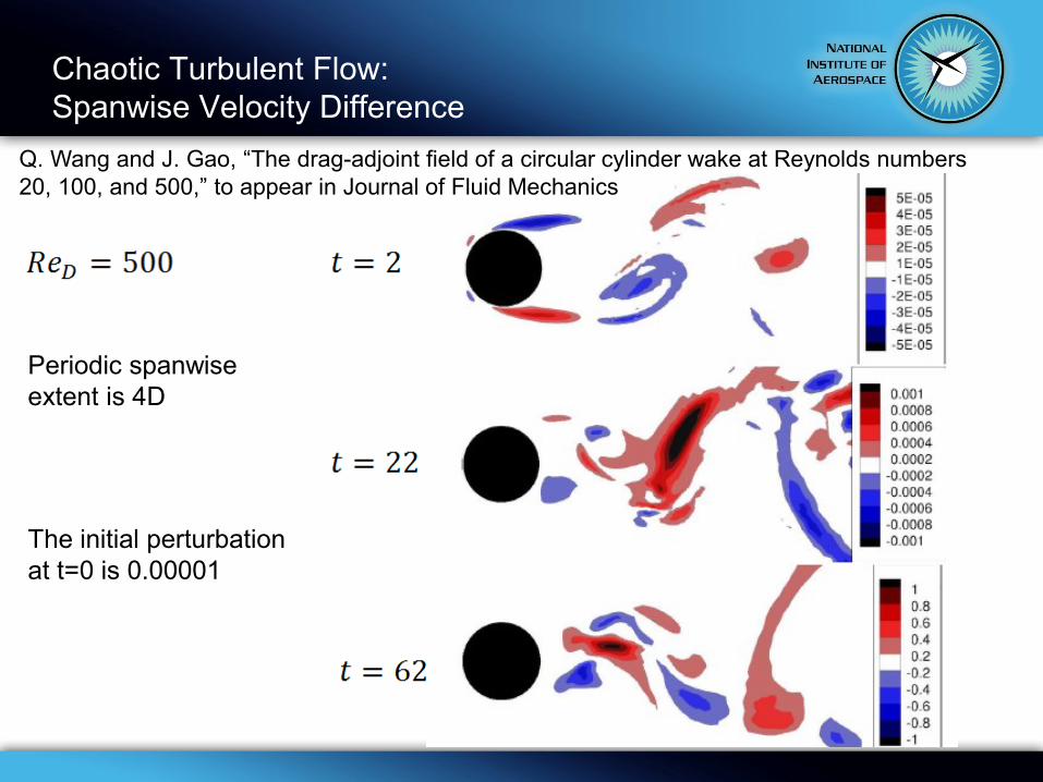
Chaotic Turbulent Flow:

Spanwise Velocity Difference

The initial perturbation

at t=0 is 0.00001

Periodic spanwise

extent is 4D

Q. Wang and J. Gao, “The drag-adjoint field of a circular cylinder wake at Reynolds numbers

20, 100, and 500,” to appear in Journal of Fluid Mechanics

Example of Linear Instability

NACA 0012 Airfoil Vorticity Contours Linear Residual L2 Norm

Challenge: Find Global Optimum

Search for the Global Minimum

• Gradient based optimization methods tend to stuck at local

minima; efficient methods for overcoming shallow local

minima and searching the global minimum are needed.

New ideas are highly appreciated!

THANK YOU!