Embed Size (px)
Citation preview
Adjoint-based optimization for optimal control problems
governed by nonlinear hyperbolic conservation laws
Elimboto Yohana
A dissertation submitted for the degree of amaster of science
School of Computational and Applied Mathematics,
University of the Witwatersrand,
Johannesburg, South Africa.
May 20, 2012
Abstract
Research considered investigates the optimal control problem which is constrained by a hy-
perbolic conservation law (HCL). We carried out a comparative study of the solutions of the
optimal control problem subject to each one of the two different types of hyperbolic relaxation
systems [64, 92]. The objective was to employ the adjoint-based optimization to minimize the
cost functional of a matching type between the optimal solution and the target solution. Nu-
merical tests were then carried out and promising results obtained. Finally, an extension was
made to the adjoint-based optimization approach to apply second-order schemes for the optimal
control problem in which also good numerical results were observed.
i
Declaration
I, the undersigned, hereby declare that this dissertation is my own, unaided work, and that any
work done by others has been acknowledged and referenced accordingly. It is being submitted
for the Degree of Master of Science at the University of the Witwatersrand, Johannesburg. It
has not been submitted before for any degree or examination to any other university.
Elimboto Yohana, May 20, 2012
Acknowledgements
I would like to thank all those who assisted me hand in hand to accomplish this project. My
grateful thanks are conveyed to Professor Mapundi Banda, being my supervisor and a close
friend, for helping me to secure funding for this research project and for his outstanding con-
tribution in terms of ideas, skills, proper direction, recommendations and motivation during
the whole period of research. I also want to thank the University of the Witwatersrand and
the African Institute for Mathematical sciences (AIMS) staff who also secured funding for my
studies. Many thanks especially, to the AIMS Director, Professor Barry Green, the former Head
of the School of Computational and Applied Mathematics (CAM), professor David Sherwell, the
current Head of School, Professor Ebrahim Momoniat and to all lecturers and researchers in the
School of CAM: Block, Charis, Conraaed, David, Joel, Montazi, Robert, just to name a few.
I would also like to extend my sincere thanks to the CAM staff members working in different ways
to sustain a facilitative and supportive living and learning environment. My special gratitudes
go to Barbie, Dorina, Keba and Wendy for their care and skillful management.
I would also like to thank my employer, the Dar Es Salaam University College of Education, a
constituent college of the university of Dar Es salaam for granting me permission to pursue this
study.
Many thanks to my friend Said Sima who worked closely with me during the whole period of
research, his advice and willingness to assist, will always make me remember him. I thank all
CAM PGD students, namely, Naval, Morgan, Gideon, Guo-Dong, Terry, Tanya, Dario, Viren,
Franklin, Obakeng, Asha, Tumelo, Charles Fodya and Innocent, for their outstanding academic
and social contribution which have made CAM school an excellent place and enchanting center
for researchers.
I highly recognize the contribution given by my family: my parents, brothers and sisters in terms
of advice, encouragement, and prayers. Since when I joined the education system, unquestion-
ably, any success in my academic advancement has their hands.
I do not want to leave behind various friends, at Johannesburg, Dar Es salaam, Cape Town and
elsewhere for their prayers, spiritual support and social advice. Special thanks goes to Rugare,
Ogana, Armstrong, Ruth, Emmanuel, Anne, Wilbert, Gerald, Davids, Greg, Mackllen, John,
Navin, Andrew, Leonard, Lois and Richard. Thanks to my friend Bwasiri for his encouragement
and valuable social advice during my stay at Wits.
All these contributions, collectively amounted to a lenient conducting of my research.
Lastly, I convey my gratitude to Almighty God for giving me strength and healthy during the
whole period of my stay at Wits.
i
Contents
Abstract i
List of Tables v
List of Figures vi
1 Introduction 1
1.1 Objectives of the Study . . . . . . . . . . . . . . . . . . . . . . . . . . . . . . . . 1
1.2 Solutions of nonlinear hyperbolic conservation laws . . . . . . . . . . . . . . . . . 2
1.3 Relaxation system . . . . . . . . . . . . . . . . . . . . . . . . . . . . . . . . . . . 5
1.4 Adjoint-based optimal control . . . . . . . . . . . . . . . . . . . . . . . . . . . . . 5
1.4.1 Organization of the work . . . . . . . . . . . . . . . . . . . . . . . . . . . 6
2 Mathematical Framework 8
2.1 Governing System of Conservation Laws . . . . . . . . . . . . . . . . . . . . . . . 8
2.2 General Hyperbolic Systems . . . . . . . . . . . . . . . . . . . . . . . . . . . . . . 10
2.2.1 Linear hyperbolic systems . . . . . . . . . . . . . . . . . . . . . . . . . . . 10
2.2.2 Nonlinear hyperbolic systems . . . . . . . . . . . . . . . . . . . . . . . . . 11
2.2.3 Diagonalization of hyperbolic systems . . . . . . . . . . . . . . . . . . . . 11
2.2.4 Transform to characteristic variables . . . . . . . . . . . . . . . . . . . . . 11
2.3 Weak Solutions . . . . . . . . . . . . . . . . . . . . . . . . . . . . . . . . . . . . . 12
2.4 Relaxation Approaches . . . . . . . . . . . . . . . . . . . . . . . . . . . . . . . . . 14
2.5 JIN XIN Relaxation Approximation Methods . . . . . . . . . . . . . . . . . . . . 14
2.5.1 Chapman-Enskog analysis for JIN XIN relaxation system . . . . . . . . . 15
2.5.2 Diagonalization of JIN XIN relaxation system . . . . . . . . . . . . . . . . 16
2.5.3 Characteristic variables for JIN XIN relaxation system . . . . . . . . . . . 17
2.6 A BGK Model . . . . . . . . . . . . . . . . . . . . . . . . . . . . . . . . . . . . . 18
2.7 Problem Formulation and Adjoint Approach to Optimization . . . . . . . . . . . 19
2.7.1 Derivation of the optimality system from JIN XIN relaxation system . . . 20
2.7.2 Derivation of the adjoint system for the discrete kinetic model . . . . . . 22
ii
3 Discretizations of the Relaxation Systems 25
3.1 Construction of the First-order JIN XIN Relaxing Scheme . . . . . . . . . . . . . 25
3.1.1 Spatial discretization . . . . . . . . . . . . . . . . . . . . . . . . . . . . . . 25
3.1.2 TVD Runge-Kutta time discretization . . . . . . . . . . . . . . . . . . . . 27
3.2 First-order Discretization of the Adjoint System . . . . . . . . . . . . . . . . . . . 28
3.2.1 Spatial discretization . . . . . . . . . . . . . . . . . . . . . . . . . . . . . . 28
3.2.2 TVD Runge-Kutta time discretization for the adjoint system . . . . . . . 29
3.3 MUSCL, TVD High Resolution Schemes: JIN XIN Relaxation Scheme . . . . . . 30
3.3.1 Construction of MUSCL, TVD second-order in space schemes . . . . . . . 30
3.3.2 TVD, Runge-Kutta second-order in time discretization . . . . . . . . . . . 32
3.4 Discretization of the Adjoint Equation, Second-order in Time and Space . . . . . 33
3.4.1 Spatial discretization . . . . . . . . . . . . . . . . . . . . . . . . . . . . . . 33
3.4.2 Time discretizations . . . . . . . . . . . . . . . . . . . . . . . . . . . . . . 35
3.5 Relaxing Scheme for the Discrete Kinetic Relaxation system . . . . . . . . . . . . 37
3.5.1 Discretization of the discrete kinetic model, first-order in time and space . 37
3.5.2 Spatial discretization for the discrete kinetic model, second-order in space 38
3.5.3 Second-order Runge-Kutta time discretizations for the discrete kinetic model 38
3.5.4 Time and space adjoint discretizations of discrete kinetic model, second-
order . . . . . . . . . . . . . . . . . . . . . . . . . . . . . . . . . . . . . . . 40
3.6 Boundary conditions . . . . . . . . . . . . . . . . . . . . . . . . . . . . . . . . . . 42
3.6.1 Periodic boundary conditions . . . . . . . . . . . . . . . . . . . . . . . . . 42
3.6.2 Transparent boundary conditions . . . . . . . . . . . . . . . . . . . . . . . 43
3.6.3 Algorithm for gradient computing . . . . . . . . . . . . . . . . . . . . . . 43
4 Numerical Results 45
4.1 Numerical Discretizations of Spatial and Temporal Domains . . . . . . . . . . . . 45
4.2 General Descriptions . . . . . . . . . . . . . . . . . . . . . . . . . . . . . . . . . . 45
4.3 Numerical Experiments for Scalar HCLs . . . . . . . . . . . . . . . . . . . . . . . 46
4.3.1 Numerical experiments for scalar linear HCLs . . . . . . . . . . . . . . . . 46
4.3.2 Numerical experiments for scalar nonlinear HCLs . . . . . . . . . . . . . . 47
4.4 Numerical Solutions for Systems of HCLs . . . . . . . . . . . . . . . . . . . . . . 50
4.5 Numerical Solutions for Nonlinear Systems of HCLs . . . . . . . . . . . . . . . . 53
iii
4.5.1 Sod Shock Tube Problem . . . . . . . . . . . . . . . . . . . . . . . . . . . 55
4.5.2 First and second order numerical tests . . . . . . . . . . . . . . . . . . . . 55
4.6 Adjoint-Optimization Tests . . . . . . . . . . . . . . . . . . . . . . . . . . . . . . 61
4.6.1 Optimization tests for scalar nonlinear HCLs . . . . . . . . . . . . . . . . 64
4.6.2 Optimization tests for systems of nonlinear HCLs . . . . . . . . . . . . . . 64
4.7 Functional Convergence . . . . . . . . . . . . . . . . . . . . . . . . . . . . . . . . 71
4.8 Comparison of Computation time . . . . . . . . . . . . . . . . . . . . . . . . . . . 71
5 Conclusions 77
iv
List of Tables
4.1 Computational time for first-order JIN XIN and discrete kinetic schemes . . . . . 76
4.2 Computational time for second-order JIN XIN and discrete kinetic schemes . . . 76
v
List of Figures
2.1 Initial solution and final solution at time = 0.5 for the linear advection equation 9
2.2 Initial and final solution of the Inviscid Burgers’ equation at time t = 0.5 . . . . 10
4.1 Solution of the linear advection equation (4.3.1) for JIN XIN scheme (black solid
line with squares at data points), kinetic scheme (green asterisk), and a reference
solution (red solid line) for a = 1, M = 400 and ε = 10−8. The x-axis represents
the space variable x and the y-axis represents the advected quantity, u. . . . . . 48
4.2 Solution of the Burgers’ Equation using JIN XIN scheme (black solid line with
squares at data points), kinetic scheme (green asterisk), and a reference solution
(red solid line) for a = 1.3, M = 400 and ε = 10−8. The x-axis represents the
space variable x and the y-axis represents the conserved quantity, u. . . . . . . . 49
4.3 First and second-order numerical solutions for JIN XIN and discrete kinetic relax-
ing schemes. The x-axis represents the space variable x and the y-axis represents
the velocity field, u. . . . . . . . . . . . . . . . . . . . . . . . . . . . . . . . . . . 51
4.4 Solution of the wave equation (4.4.5), JIN XIN scheme (black solid line with
squares at data points), kinetic scheme (green asterisk), and exact solution (red
solid line); T = π2 , M = 400, ε = 10−8, a = 1. The x-axis represents the space
variable x and the y-axis represents the wave profile, u. . . . . . . . . . . . . . . 53
4.5 Sketch of the initial configuration of the shock tube at time t = 0. PL, TL, VL
and PR, TR, VR are, respectively pressure, temperature and velocity; on the left
and right part of the tube. . . . . . . . . . . . . . . . . . . . . . . . . . . . . . . . 56
4.6 Sketch of the shock tube showing waves interaction after the membrane break-
down, t > 0. . . . . . . . . . . . . . . . . . . . . . . . . . . . . . . . . . . . . . . . 57
4.7 First and second order numerical solutions for density, velocity and pressure pro-
files with JIN XIN and discrete kinetic schemes, for 1D Euler Equations at time,
T = 0.17, uL = (1.25, 0.0, 1.2), uR = (0.25, 0.0, 0.25), for a1 = 1.0, a2 =
2.5, a3 = 5.2, M = 400 and ε = 10−8. The x-axis represents the space variable x
and the y-axis represents density (top), velocity (middle) and pressure (bottom). 58
4.8 First and second order numerical solutions for density, velocity and pressure pro-
files with JIN XIN and discrete kinetic schemes, for 1D Euler Equations at time,
T = 0.17, uL = (1.45, 0.0, 1.5), uR = (0.45, 0.0, 0.5); a1 = 2.2, a2 = 2.5, a3 =
5.0, M = 400 and ε = 10−8. The x-axis represents the space variable x and the
y-axis represents density (top), velocity (middle) and pressure (bottom). . . . . . 59
vi
4.9 First and second order numerical solutions for density, velocity and pressure pro-
files with JIN XIN and discrete kinetic schemes, for 1D Euler Equations at time,
T = 0.17, uL = (2.5, 0.0, 2.0), uR = (0.5, 0.0, 0.6); a1 = 3.5, a2 = 4.5, a3 = 5.5,
M = 400 and ε = 10−8. The x-axis represents the space variable x and the y-axis
represents density (top), velocity (middle) and pressure (bottom). . . . . . . . . . 60
4.10 Comparing first-order and second-order solutions for different grids with JIN XIN
scheme; T = 0.17, uL = (2.5, 0.0, 2.0), uR = (0.5, 0.0, 0.6); a1 = 2.0, a2 =
3.5, a3 = 5.5, ε = 10−8. The x-axis represents the space variable x and the y-axis
represents density (top), velocity (middle) and pressure (bottom). . . . . . . . . . 62
4.11 Comparing first-order and second-order solutions for different grids with discrete
kinetic scheme. Same parameters as in Figure 4.10. The x-axis represents the
space variable x and the y-axis represents density (top), velocity (middle) and
pressure (bottom). . . . . . . . . . . . . . . . . . . . . . . . . . . . . . . . . . . . 63
4.12 First-order adjoint-based optimization of scalar nonlinear HCL results for JIN
XIN and kinetic schemes, M = 400 and ε = 10−8. The x-axis represents the
space variable x and the y-axis represents the conserved quantity, u. . . . . . . . 65
4.13 Same parameters as in Figure 4.12 but second-order tests. The x-axis represents
the space variable x and the y-axis represents the conserved quantity, u. . . . . . 66
4.14 First-order (Left) and second-order (Right) 1D Euler Equations optimal control
results. The optimal solution is shown by the red solid line and target by black
solid line with squares at data points, T = 0.17, uL = (1.2, 0.078, 1.2), uR =
(0.325, 0.285, 0.295), a1 = 2.183, a2 = 3.004, a3 = 4.286, M = 400 and ε = 10−8.
The x-axis represents the space variable x and the y-axis represents density (top),
velocity (middle) and pressure (bottom). . . . . . . . . . . . . . . . . . . . . . . . 67
4.15 First-order (Left) and second-order (Right) 1D Euler Equations optimal control
results obtained with discrete kinetic scheme. Optimal solution is depicted by
the red solid line and target by black solid line with squares at data points, same
parameters as used for Figure 4.14. The x-axis represents the space variable x
and the y-axis represents density (top), velocity (middle) and pressure (bottom). 68
4.16 First-order (Left) and second-order (Right) 1D Euler Equations optimal control
results. Optimal (red solid line) and target (black solid line with squares at data
points) solutions, for density, velocity and pressure profiles with JIN XIN scheme
at time, T = 0.17, uL = (1.2, 0.2, 1.25), uR = (0.32, 0.73, 0.32), a1 = 2.47, a2 =
3.5, a3 = 4.36, M = 400 and ε = 10−8. The x-axis represents the space variable
x and the y-axis represents density (top), velocity (middle) and pressure (bottom). 69
vii
4.17 First-order (Left) and second-order (Right) 1D Euler Equations optimal control
results. Optimal (red solid line) and target (black solid line with squares at data
points) solutions, for density, velocity and pressure profiles with discrete kinetic
scheme. Same parameters as in Figure 4.16. The x-axis represents the space
variable x and the y-axis represents density (top), velocity (middle) and pressure
(bottom). . . . . . . . . . . . . . . . . . . . . . . . . . . . . . . . . . . . . . . . . 70
4.18 First-order (Left) and second-order (Right) 1D Euler Equations optimal control
results. Optimal (red solid line) and target (black solid line with squares at
data points) solutions, for density, velocity and pressure profiles with JIN XIN
scheme at time; T = 0.17, uL = (1.24, 0.1852, 1.25), uR = (0.366, 0.629, 0.33),
a1 = 1.96, a2 = 2.9, a3 = 4.33, M = 400 and ε = 10−8. The x-axis represents
the space variable x and the y-axis represents density (top), velocity (middle) and
pressure (bottom). . . . . . . . . . . . . . . . . . . . . . . . . . . . . . . . . . . . 72
4.19 First-order (Left) and second-order (Right) 1D Euler Equations optimal control
results. Optimal (red solid line) and target (black solid line with squares at
data points) solutions, for density, velocity and pressure profiles obtained with
the discrete kinetic scheme. Same parameters as in Figure 4.18. The x-axis
represents the space variable x and the y-axis represents density (top), velocity
(middle) and pressure (bottom). . . . . . . . . . . . . . . . . . . . . . . . . . . . 73
4.20 First-order (Left) and second-order (Right) 1D Euler Equations optimal control
results. Optimal (red solid line) and target (black solid line with squares at data
points) solutions, for density, velocity and pressure profiles with JIN XIN scheme
at time, T = 0.17, uL = (1.0, 0.0, 1.0), uR = (0.1, 0.0, 0.125) for optimal; and
uL = (1.1, 0.0, 1.1), uR = (0.2, 0.0, 0.2) for target. a1 = 1.96, a2 = 2.9, a3 =
4.33, M = 400 and ε = 10−8. The x-axis represents the space variable x and the
y-axis represents density (top), velocity (middle) and pressure (bottom). . . . . . 74
4.21 First-order (Left) and second-order (Right) 1D Euler Equations optimal control
results. Optimal (red solid line) and target (black solid line with squares at data
points) solutions, for density, velocity and pressure profiles with discrete kinetic
scheme at time, T = 0.17. Same parameters as in Figure 4.20. The x-axis
represents the space variable x and the y-axis represents density (top), velocity
(middle) and pressure (bottom). . . . . . . . . . . . . . . . . . . . . . . . . . . . 75
4.22 Convergence history for the solution of the optimization problem computed with
the first order (left) and second-order (right) relaxing schemes for both JIN XIN
and discrete kinetic schemes. The x-axis represents the number of iterations and
the y-axis represents the cost functional value. . . . . . . . . . . . . . . . . . . . 76
viii

1. Introduction
Hyperbolic conservation laws (HCLs) is an active research field with rapidly increasing appli-
cations in areas such as fluid mechanics, aircraft designs, traffic flows, elasticity and relativity.
This work is devoted to discuss the mathematical framework and numerical solutions for the
adjoint-based optimization of the optimal control problem subject to one-dimensional relaxation
systems of HCLs. We are interested in the numerical solutions of optimization problems gov-
erned by a system of hyperbolic conservation laws (HCLs). The approach under consideration
is called adjoint, and in this case, it requires solutions of two systems of equations in each
optimization cycle, as it is explained in the later sections.
Since 1970s, there has been intensive research in the field of HCLs. This research has accelerated
the applications of HCLs in fields such as Computational Fluid Dynamics (CFD) [89]. HCLs
are very important in our daily life because they model different sorts of physical processes.
Several studies conducted led to successful application of HCLs in science [27, 82], technology of
combustion, detonation, aerodynamic designs and gas dynamics [49, 125], to name only a few.
Today, there is a lot of research which aims to apply HCLs in solving challenging problems in
engineering and science (reactive flows, multi-component flows, groundwater flows, semiconduc-
tors and meteorology), economical and industrial platforms. There are typical applications of
HCLs, such as Buckley Leverett [126] in modeling flows in oil and gas reservoirs, the shallow
water equations in meteorology and oceanography, equations of magnetohydrodynamics (MHD)
in studying supernovas in astrophysics, also applied in plasma physics, solid mechanics; and
Euler Equations in aircraft designs and traffic flow models [4, 79, 126]. Some other references
on successful applications of HCLs are found in [63].
Apart from numerous existing literature on the relaxation approach to solutions of HCLs, to
our knowledge, few reports are available on the optimal control problems subject to relaxation
systems. In this study, we investigated two relaxation approaches as constraints to the opti-
mization problem (to be defined later), namely: the JIN XIN relaxation approach [64], and the
discrete velocity model approach in [5, 92]. Contrary to the existing results in [10, 94, 128], we
have extended the adjoint method to second-order relaxing schemes for numerical optimization
of the problem governed by nonlinear scalar and systems of HCLs. Effective relaxation ap-
proaches have been developed and their performances compared in connection to adjoint-based
optimization. The aim is to minimize the cost functional that matches the optimal solution and
the target, subject to this set of relaxation systems.
1.1 Objectives of the Study
Objectives for this study are as follows:
1
Section 1.2. Solutions of nonlinear hyperbolic conservation laws Page 2
• to derive optimality systems for the two variants of the relaxation system: the JIN XIN
relaxation approach, [64] and the discrete kinetic model [92]. The optimality system is
comprised of the systems of equations, namely: state equations, the co-state equations and
the optimality condition, which are then discretized in the numerical implementation;
• to derive first-order relaxing schemes and test them by solving different systems of HCLs,
including the real world examples and apply these solution procedures to the problem
of optimal control. The interest has been to realize the more computationally effective
approach, challenging them, pointing out drawbacks and giving suggestions whenever nec-
essary. We have comparatively checked the validity of the two approaches and drawn
conclusions based on their numerical results;
• Investigation of the application of second-order relaxing schemes for the solutions of HCLs
and for the optimal control problem as well.
Successful optimization in this sense, depends on suitable approach used to approximate solu-
tions of HCLs. HCLs exhibit unique behavior and require special treatment, (see [18, 33, 67,
69, 75, 78, 126]) for their solutions. Generally, numerical schemes for hyperbolic conservation
laws available in the literature are numerous. In this regard, it is not possible to explore all
of them under this limited space, but in the following section, we discussed some common and
frequently used numerical methods for solutions of HCLs.
1.2 Solutions of nonlinear hyperbolic conservation laws
In the past decades, numerous numerical methods have been developed to solve nonlinear hyper-
bolic conservation laws. The most challenging feature of the nonlinear hyperbolic conservation
laws is the development of singularities as their solution evolves with time. These singularities
which are jumps are also called shock waves. In general, the property of nonlinear hyperbolic
conservation law is that, even if the solution at a given time is smooth, it may in general develop
discontinuities at a later time.
Different methods have been used to solve HCLs, with some attempts to generalize solution
approaches to high orders of accuracy. For many years, traditional numerical schemes have been
used to solve partial differential equations (PDEs). Most of these schemes are not suitable for
solving PDEs especially when the function is discontinuous as their solutions, often result into
over-smeared representation of shocks or oscillations near discontinuities [121]. Under nonlinear
conservation laws (CLs) for example, some schemes fail to capture the correct direction of infor-
mation propagation yielding incorrect or oscillatory solutions. There are well known methods
under this category, namely, Lax-Wendroff second-order method [108], upwind method [109],
Godunov’s method [47], methods of Hyman [61], MacCormack method [85], Rusanov method

Section 1.2. Solutions of nonlinear hyperbolic conservation laws Page 3
[111], method of Boris and Book [16], method of Harten and Zwas [54], Glimm’s method [32]
and the random choice method [33]. These methods rely on approximation of derivatives ap-
pearing in the differential equations by finite difference method (FDM) [130, 131], finite volume
method (FVM) [29, 123] or finite element method (FEM) [30, 31, 66] to obtain discrete forms of
PDEs. Detailed discussion on these methods with applications in some cases is found in [106],
and basics for the conservation laws-based ideas were discussed in [76].
It is preferred and it has been found valuable to use finite volume methods [77] in the setting of
nonlinear hyperbolic conservation laws. The Godunov’s method that was introduced in [47] for
the purpose of solving the Euler Equations of gas dynamics in the presence of discontinuities for
example, is probably the most appealing finite volume approach. Although the derivation of both
finite difference and finite volume methods may be quite different, the resulting representation
formulae may be identical, but normally, each method is interpreted differently. Finite volume
methods involve solutions of Riemann problems. There are well known and frequently used
approximate Riemann solvers [125] in finite volume or high-resolution methods reported in
various papers and books: The all-shock solver [32], Osher Solver [100], which is an extension
of the Engquist-Osher method [39, 40, 41] derived for scalar conservation laws, the HLLE solver
[57] and its improvement in [36], and the Roe solver scheme [110]. Riemann problems are usually
computationally costly, and one would therefore like to devise a method that avoids solution of
the Riemann problem.
Finite volume methods like Godunov’s method are at most first-order accurate on smooth regions
of solution and in general, these methods perform poorly near or at shock waves or other
discontinuities giving very smeared approximations. An improvement is made by developing a
method which can be interpreted as a correction phase to the solution of the Riemann problem
and through reconstruction of the finite volume fluxes to obtain high-resolution versions of
the finite volume methods. High-resolution methods resolve discontinuities more sharply and
produce at-least second-order accurate solutions in smooth regions of the flow at the same time
trying to remain faithful to the physics of the problem by avoiding nonphysical oscillations near
discontinuities. Most high-resolution methods for capturing shocks are based on solutions of
Riemann problems between states in neighboring grid cells. Numerous literature rich in history
and development of these methods is presented in various books [1, 46, 65, 76, 107, 120, 125].
Second-order methods include for example, Monotone upstream-centred Scheme (MUSCL) [71,
72, 73] and flux-corrected transport (FCT) algorithms by Boris and Book [16] for nonlinear
conservation laws.
The class of high-resolution methods also includes high-order accurate finite difference essentially
non-oscillatory (ENO) [53, 55, 58, 133, 134] and its extension, weighted ENO [26, 43, 83, 101, 116]
schemes designed for problems with piecewise smooth solutions containing discontinuities [119].
ENO and WENO schemes use nonlinear adaptive procedure to automatically choose the locally
Section 1.2. Solutions of nonlinear hyperbolic conservation laws Page 4
smoothest stencils in order to avoid interpolating across discontinuities. The class of these
schemes has been successful applied to problems containing shocks as well for smooth solutions
with complex structures. ENO and WENO methods are among of the more recent classes
which efficiently solve hyperbolic conservation laws. Stable spatial discretization for hyperbolic
conservation laws with high-resolution schemes such as ENO [133, 134] and WENO [26, 43, 101]
are usually applied in combination with strong stability-preserving (SSP) time discretizations
methods discussed below.
Most of these numerical approaches to PDEs, especially HCLs uses semi-discrete methods. These
approaches first discretize the PDE in space to obtain a system of ordinary differential equations
(ODEs) while retaining continuous time. The ODE is then discretized in time by an appropriate
ODE method, typically TVD [48, 54, 56, 98, 99, 117, 118, 124] or SSP [49, 50, 117, 119] Runge-
Kutta methods [50, 52, 112, 113, 119]. For Runge-Kutta schemes, one may decide to use multi-
level [62, 90] or one-step methods. Multi-level schemes, such as TVD high-order Runge-Kutta
time discretizations are rarely used in practice because they are not self starting in the sense
that they may need other methods at initial levels to get started. However, these methods
may also require large storage during computations. As a result, usually one-step Runge-Kutta
TVD methods are preferable because they need low storage and are self starting. Low storage
Runge-Kutta methods are discussed in [25, 132]. The advantage of semi-discrete method is that
high-order accuracy in space and time can be achieved through a decoupled process, making
them much simpler than the fully discrete ones. Due to this reason, high-order schemes, such
as Runge-Kutta type time discretizations can easily be applied in combination with different
spatial discretizations.
TVD Semi-discrete schemes in combination with Runge-Kutta methods have been a success
story in many numerical applications. It has been shown in [48], even if linearly stable, non-
TVD Runge-Kutta methods may develop oscillations. It is, therefore, recommended to always
maintain TVD property in both time and spatial discretizations for high-order schemes. SSP
methods have been widely applied in many areas, some of them include compressible flow [130],
incompressible flow [105], viscous flow [123], atmospheric transport [29]. For a complete list of
references on applications of SSP methods, an interested reader may consult [49].
There is another numerical approach analogous to Godunov’s method based on flux-vector
splitting which evaluates fluxes at the cell average discussed in [78]. Mathematical discussion
based on this approach is found in various literature referenced in [78]. Equivalent flux-vector
splitting approaches have since then been developed, they include Steger-Warming [122], Beam
scheme [115], the Marquina flux [35, 86], and the one introduced in [74], followed by a number
of other variants and improvements reported in [80, 81].
Section 1.3. Relaxation system Page 5
1.3 Relaxation system
We considered relaxation approximation to HCLs as was first discussed in [64]. Since the first
introduction in [64], numerous discussion on relaxation schemes have been emerging [13, 10, 17,
94, 116]. Analysis on the existence and uniqueness of the solution for the relaxation approach
described in [64] was given in [129].
A different relaxation framework has been introduced in [6, 5]. This relaxation system basically
takes the form of the discrete BGK [14] model approximation. Under this relaxation setting,
estimates on the discrete schemes as well as convergence analysis for first-order and second-order
spatial dimensions have been studied [6]. Further study is found in [88, 91, 92, 93].
Relaxation methods are based on the replacement of the nonlinear systems of HCLs on a con-
tinuous level (before any kind of discretization) by a semilinear system with a stiff relaxation
source term. This system reverts to the original conservation law as the relaxation parameter
tends to zero. Convergence analysis for scalar hyperbolic conservation law has been fully real-
ized. The case of systems is an ongoing research problem. In numerical computation, our focus
is on relaxing schemes which are the limits for small positive relaxation parameter.
We have chosen the relaxation method due to its promising features of simplicity which can lead
to generalization to both higher orders and high dimensional systems of HCLs without further
modification. However, relaxation approximation preserves the hyperbolic nature of the system
on the expense of additional source terms and additional equations. The semilinearity structure
of the relaxation system allows for Riemann-solvers free treatment and avoids the computation of
Jacobians. All these features make this method incredibly advantageous especially in situations
where Jacobians and Riemann problems are difficult to solve [64].
1.4 Adjoint-based optimal control
There is a lot of theoretical and numerical discussion of hyperbolic conservation laws in the
optimal control setting. It is well known that a flow generated by hyperbolic conservation laws
is not differentiable with respect to the linear structure of L1 even for scalar 1D case [10, 21].
A generalized notion of differential structure for maps taking values within a class of piecewise
Lipschitz functions was studied in [22], and the flow generated by a HCL was proven to be
differentiable in this generalized sense. The list of papers [15, 19, 20] discuss the notion of shift
differentiability of the flow generated by a system of conservation law. The latter two papers also
introduce a new differential structure on the BV space of integrable functions having bounded
variation. It is also shown in [19], that the flow generated by a scalar conservation law is generally
differentiable with respect to this new introduced structure. Adjoint and sensitivity calculus
based on shift differentiability in the optimal control of entropy solutions of scalar conservation
Section 1.4. Adjoint-based optimal control Page 6
laws with source term is discussed in [127]. First-order necessary optimality conditions for
systems of conservation laws are given in [23]. This discussion on differentiability of conservation
laws is motivated by its applications in the optimal control problems.
HCLs are highly applied in the optimal control problems [15, 20, 22, 84, 127] - finding some
geometry that optimizes performance subject to a set of constraints [44]. Applications of con-
servation laws in optimization are becoming more prominent in traffic flow, turbulent flow, gas
dynamics, trajectory planning and in aircraft designs. Discussion on adjoint-based optimization
of problems governed by partial differential equations (PDEs) is presented in [45, 51]. Many
adjoint-based softwares for CFD have been developed by different pioneers. These include:
adjoint-based optimal designs with an application to designing business jets [44], adjoint ap-
proach to aerodynamic designs [37, 38], adjoint approach to shape and airfoil designs [2, 24] and
continuous adjoint formulation [3, 95]. For trade-off between continuous and discrete adjoint
approach to automatic aerodynamic optimization, consult [89].
Several authors including [60] have employed the nonsmooth optimization in combination with
the adjoint methods for subgradient computation. They studied the optimal control of flows with
discontinuities and tested the approach using one dimension (1D) Riemann problem of Euler
Equations. In the cases where gradient-based methods were employed, either discontinuities
were ignored or means to circumvent their effects were employed. In many situations shocks
were smoothed using numerical dissipation. It has been shown that smoothing is sometimes
equivalent to modifying the cost function [87].
In realistic situations one has to deal with nonlinear systems. The nonlinearity in systems of
HCLs poses both analytical and numerical difficulties to their solutions due to discontinuities
that may arise. Since it is generally known that the semi-group generated by a HCL is not
differentiable in L1 even in the scalar, 1D case [10]; and the solution of HCL is needed in the
optimization cycle, it is therefore important to pay close attention to its solution.
The adjoint approach is robust in the sense that all sensitivities are calculated only once via
the adjoint equation in each iteration cycle regardless of the number of control parameters [51].
In combination with the adjoint approach, the relaxation method becomes more appealing.
However, the adjoint approach avoids unnecessary repetition which we would encounter if we
would have opted to use sensitivity-based optimization, hence may reduce CPU time and memory
required for storage.
1.4.1 Organization of the work
To this point, the scope, and plan of the work are outlined as follows: The next Chapter is
devoted to discuss useful mathematical and physical notions that are important for this study.
It is very important to clearly understand the physics of the problem since this serves as a
Section 1.4. Adjoint-based optimal control Page 7
fundamental tool to successfully solve numerically an optimization problem. This is particularly
true because numerical solutions of the optimization problem and that of HCLs are a coupled
process, in the sense that, the optimization cannot be achieved independently of the solution of
HCL. It is known that discontinuities may arise in the solution of HCL; thus both mathematical
and physical analysis must be carried out correctly prior to numerically solving HCLs. We
therefore discussed general physical and mathematical behavior underlying the HCLs. It is in
this Chapter, where we introduced and discussed the concept of adjoint-based optimization.
Next, we presented a brief mathematical explanation of relaxation systems, for both relaxation
approximation and the discrete kinetic model. Finally, we discussed and applied the Lagrangian
approach to derive optimality systems based on relaxation approaches for the two variants of
the relaxations: the JIN XIN [64] and the discrete kinetic model [92]. The derived optimality
systems then help in determining the gradients of the cost functional during the numerical
optimization process. Optimality system is comprised of the flow equations, the adjoint system
and the optimality conditions. In Chapter three, we centered our discussion on derivation of
relaxing schemes. Under this Chapter, relaxing schemes from the two relaxation approaches
mentioned previously were constructed. For iterative optimization process, we had to discretize
equations that comprise the optimality systems. Thus discretization is done under this Chapter,
where we use the method of lines (MOL) to discretize the systems of flow and adjoint equations.
With the MOL, we proceeded by discretizing the spatial domain while retaining the relaxation
HCL continuous in time, to form systems of ODEs, and then we suitably discretized in time by
appropriately applying Runge-Kutta methods. For time discretization, we used TVD Runge-
Kutta methods, where as for first-order spatial discretization, a simple upwind method is applied.
Total variation diminishing (TVD) monotone upstream-centered schemes (MUSCL) scheme was
constructed for second-order spatial discretizations by using minmod slope-limiter. In Chapter
four, we presented and discussed numerical results for both solutions of HCLs and the optimal
control problem. Optimal control results obtained by applications of both first-order and second-
order relaxing schemes are presented in this Chapter. The two approaches are compared and
conclusions drawn based on obtained numerical results. In Chapter five, a brief remark and
general conclusions based on the achieved outcomes were given. Finally, we pointed out the
possibilities for future extension of this research as well as challenges that may be encountered.
.
2. Mathematical Framework
2.1 Governing System of Conservation Laws
Conservation laws (CLs) are usually time-dependent systems of partial differential equations.
They describe the conservation of quantities such as mass, momentum and energy, and are
usually nonlinear if they have to model most of the dynamic situations. These equations are
hyperbolic in nature. In one dimensional space, the equations take the form
ut + f(u)x = 0, u(x, t = 0) = u0(x), t ∈ [0,∞), x ∈ (−∞,∞) (2.1.1)
where u : RxR+ → Rm is a vector with m conserved quantities uj , and f : Rm → Rm is the
vector-valued function called the flux function, in which each jth component fj(u) is a function
of components uj of u. The equation is called scalar when m = 1. Equations of type (2.1.1)
often describe transport phenomena and they are popularly referred to as the Cauchy problems.
If we integrate equation (2.1.1) over a given subdomain [x1, x2], we obtain
d
dt
∫ x2
x1
u(x, t)dx =
∫ x2
x1
ut(x, t)dx (2.1.2)
= −∫ x2
x1
f(u(x, t))xdx
= f(u(x1, t)− f(u(x2, t)) = [inflow at x1]− [outflow at x2]. (2.1.3)
Hence, the primal formulation of the typical conservation law (2.1.1) stipulates that the time
rate of change in the amount of quantity u inside any given interval [x1, x2] is balanced by the
rate of flux of this quantity through the boundary points of the subdomain. The only change in
u is due to the quantity entering or leaving the domain of interest through the boundaries.
The more general system (2.1.1) is called hyperbolic if the mxm Jacobian matrix of its flux
function f(u), for values of
u =
u1
u2
.
.
.
um
, and f(u) =
f1
f2
.
.
.
fm
(2.1.4)
8
Section 2.1. Governing System of Conservation Laws Page 9
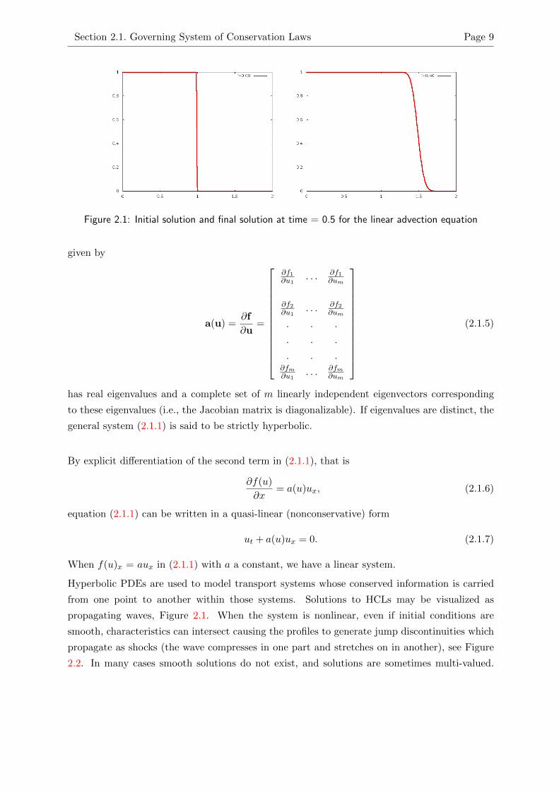
Figure 2.1: Initial solution and final solution at time = 0.5 for the linear advection equation
given by
a(u) =∂f
∂u=
∂f1∂u1
. . . ∂f1∂um
∂f2∂u1
. . . ∂f2∂um
. . .
. . .
. . .∂fm∂u1
. . . ∂fm∂um
(2.1.5)
has real eigenvalues and a complete set of m linearly independent eigenvectors corresponding
to these eigenvalues (i.e., the Jacobian matrix is diagonalizable). If eigenvalues are distinct, the
general system (2.1.1) is said to be strictly hyperbolic.
By explicit differentiation of the second term in (2.1.1), that is
∂f(u)
∂x= a(u)ux, (2.1.6)
equation (2.1.1) can be written in a quasi-linear (nonconservative) form
ut + a(u)ux = 0. (2.1.7)
When f(u)x = aux in (2.1.1) with a a constant, we have a linear system.
Hyperbolic PDEs are used to model transport systems whose conserved information is carried
from one point to another within those systems. Solutions to HCLs may be visualized as
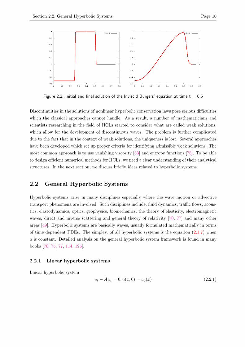
propagating waves, Figure 2.1. When the system is nonlinear, even if initial conditions are
smooth, characteristics can intersect causing the profiles to generate jump discontinuities which
propagate as shocks (the wave compresses in one part and stretches on in another), see Figure
2.2. In many cases smooth solutions do not exist, and solutions are sometimes multi-valued.
Section 2.2. General Hyperbolic Systems Page 10
Figure 2.2: Initial and final solution of the Inviscid Burgers’ equation at time t = 0.5
Discontinuities in the solutions of nonlinear hyperbolic conservation laws pose serious difficulties
which the classical approaches cannot handle. As a result, a number of mathematicians and
scientists researching in the field of HCLs started to consider what are called weak solutions,
which allow for the development of discontinuous waves. The problem is further complicated
due to the fact that in the context of weak solutions, the uniqueness is lost. Several approaches
have been developed which set up proper criteria for identifying admissible weak solutions. The
most common approach is to use vanishing viscosity [33] and entropy functions [75]. To be able
to design efficient numerical methods for HCLs, we need a clear understanding of their analytical
structures. In the next section, we discuss briefly ideas related to hyperbolic systems.
2.2 General Hyperbolic Systems
Hyperbolic systems arise in many disciplines especially where the wave motion or advective
transport phenomena are involved. Such disciplines include; fluid dynamics, traffic flows, acous-
tics, elastodynamics, optics, geophysics, biomechanics, the theory of elasticity, electromagnetic
waves, direct and inverse scattering and general theory of relativity [70, 77] and many other
areas [49]. Hyperbolic systems are basically waves, usually formulated mathematically in terms
of time dependent PDEs. The simplest of all hyperbolic systems is the equation (2.1.7) when
a is constant. Detailed analysis on the general hyperbolic system framework is found in many
books [70, 75, 77, 114, 125].
2.2.1 Linear hyperbolic systems
Linear hyperbolic system
ut +Aux = 0, u(x, 0) = u0(x) (2.2.1)
Section 2.2. General Hyperbolic Systems Page 11
where u : R×R+ → Rm and A ∈ Rm×m is a constant matrix, is called a system of conservation
laws with the flux function f(u) = Au. The system is called hyperbolic if A is diagonalisable
with real eigenvalues; and is called strictly hyperbolic when eigenvalues are distinct. This system
is simple and serves as a model for studying more general hyperbolic systems.
2.2.2 Nonlinear hyperbolic systems
The most outstanding challenge many scientists and researchers face when solving nonlinear
hyperbolic systems is the tendency of their solutions to develop shock waves. These waves
normally develop as abrupt jumps. Therefore, the most distinguished nonlinear feature is the
breaking of the solution waves into shocks. The simplest of the nonlinear hyperbolic system is
the first-order PDE (2.1.7).
2.2.3 Diagonalization of hyperbolic systems
Matrix (or systems) diagonalization is important in physics and engineering and it has common
applications in such areas as stability analysis, the physics of rotating bodies and small oscilla-
tions of vibrating systems. In order to analyze and solve the general system (2.2.1), it had been
found useful to transform the dependent variables u(x, t) to another set of dependent variables
v(x, t).
In order to be able to illustrate the concept of diagonalization and make this transformation,
we consider an arbitrary matrix A in a general linear hyperbolic system (2.2.1). A matrix A is
said to be diagonalizable if it can be expressed as
A = RDR−1 (2.2.2)
where D = (λ1, . . . , λm) is a diagonal matrix of eigenvalues and R = [r1, . . . , rm] is the matrix
of right eigenvectors corresponding to the eigenvalues λi of A. From (2.2.2), AR = RD; that’s
Arp = rpλp where p = 1, . . . ,m.
A system (2.2.1) is said to be diagonalizable if the coefficient matrix A is diagonalizable.
2.2.4 Transform to characteristic variables
The concept of characteristic variables can be well understood by considering the general linear
hyperbolic framework (2.2.1). We follow the same presentation style adapted by Toro [125] and
LeVeque [75] for this discussion.
Multiplying (2.2.1) by R−1 and substituting A = RDR−1 we get
R−1ut +R−1(RDR−1)ux = 0. (2.2.3)
Section 2.3. Weak Solutions Page 12
Since R−1 exists, we can define new set of dependent variables v = (v1, . . . , vm), and through
transforming v = R−1u, we have
vt +Dvx = 0. (2.2.4)
The new variables v are called characteristic variables. D is diagonal, so (2.2.4) results (de-
couples) into m independent scalar equations
(vp)t + λp(vp)x = 0, p = 1, . . . ,m. (2.2.5)
Each of these equations is a linear advection equation with a constant coefficient, whose solution
(by method of characteristics) is
vp(x, t) = vp(x− λpt, 0). (2.2.6)
When we write the system (2.2.4) in full it becomes
v1
v2
.
.
.
vm
t
+
λ1 . . . 0
0 . . . 0
. . .
. . .
. . .
0 . . . λm
v1
v2
.
.
.
vm
x
= 0. (2.2.7)
These are governing PDEs in terms of characteristic variables. The characteristic speed is λi
and there are m characteristic curves satisfying m ordinary differential equations (ODEs)
xt = λp, p = 1, . . . ,m. (2.2.8)
This is useful information that is needed for transformation of a relaxation system (2.5.2). In
the next section, we considered what is called weak solutions to (2.1.1).
2.3 Weak Solutions
We consider a Cauchy (initial-value problem (IVP)) for scalar conservation laws in one space
dimension ut + f(u)x = 0 in R× (0,∞)
u(x, t) = u0(x) on R× t = 0,(2.3.1)
f : R → R and u0 : R → R are given and the unknown is, u(x, t) = u : R × [0,∞) → R.
As it is known, the method of characteristics (MOC) is the classical method for solving the
Section 2.3. Weak Solutions Page 13
IVP for the general first-order PDE with two independent variables. The goal of the MOC
when applied to a PDE is to reduce it to an ODE along some characteristic curves, and the
ODE can then be integrated to obtain the desired solution. Singularities are inevitable to the
solution of the hyperbolic conservation law (2.3.1), and it is proven in literature [42] that, there
does not, in general, exist a smooth solution of (2.3.1) for all times t > 0; smooth solution can
only exist locally. Since we are interested in the global behavior of this solution, we need to
re-formulate the problem by setting a general framework that allows some sort of generalized
or weak solutions. Weak solutions are not classical [4], not necessarily differentiable, and they
satisfy CLs point-wise. Weak solutions are also not necessarily unique and they may not be
physical. Due to that, extra conditions such as Oleinik entropy condition [97] and Lax’s entropy
condition [68], which narrows down weak solutions; singling out admissible ones may need to
be imposed. The reader may refer to various existing standard literature such as [33, 42] for
classical treatment of weak solutions.
Since we cannot in general find a classical solution of (2.3.1), we must devise some means to
solve for a more general solution u which is the solution of an IVP (2.3.1). We can achieve
this by temporarily assuming u is smooth and multiply the PDE (2.3.1) by an arbitrary test
function Φ with continuous first derivatives, in R and then to integrate by parts, so that we can
transfer the derivatives onto Φ. Our test functionΦ : R× [0,∞)→ R is smooth, with
compact support,(2.3.2)
that means the function vanishes outside or on the boundaries of the compact subset of the
domain of interest. Now we multiply the PDE (2.3.1) by Φ. Integrating the equation (2.3.3),
0 =
∫ ∞0
∫ ∞−∞
(ut + f(u)x)Φdxdt (2.3.3)
by parts (Using Fubini’s Theorem), we have
(2.3.4)−∫ ∞
0
∫ ∞−∞
uΦtdxdt+
∫ ∞−∞
uΦ|∞0 dx−∫ ∞
0
∫ ∞−∞
f(u)Φxdxdt+
∫ ∞0
f(u)Φ|∞−∞dt = 0.
We assume that Φ vanishes near the boundaries of R, and with the initial condition u = u0(x)
on R× t = 0, we obtain the identity∫ ∞0
∫ ∞−∞
uΦt + f(u)Φxdxdt+
∫ ∞−∞
u0(x)Φ(x, 0)dx = 0. (2.3.5)
Weak solutions will be employed in the derivation of the adjoint systems to the relaxation
systems that we consider in the subsequent sections.
Section 2.4. Relaxation Approaches Page 14
2.4 Relaxation Approaches
The aim of relaxation approach is to transform a nonlinear conservation law into a system of
linear convective equations with a nonlinear source term. A good approximation to the original
conservation law is achieved by solving relaxation system for a positive parameter ε 1. Such
relaxation systems are stiff. The relaxation method replaces a nonlinear system by a semilinear
system with great advantage that it can be solved numerically by avoiding computationally costly
Riemann solvers. Here, we have considered two classes of relaxation approaches, namely the
relaxation approximation [64] and the discrete kinetic model [5] for the purpose of optimization.
2.5 JIN XIN Relaxation Approximation Methods
We choose relaxation approach [6, 10, 28, 64, 116] because of its simplicity and easy generaliza-
tion; that is, the system is easily extended to high-order schemes or multi-dimensional systems
and their solutions can be treated similarly like in scalar 1D case. It has also been noted that,
relaxation schemes preserve the hyperbolic structure on the expense of additional terms. How-
ever, semi-linearity is perhaps the most attractive feature of relaxation structure which allow for
Riemann-solvers free treatment. We consider the model Riemann - Cauchy problem (the IVP
with piecewise constant data), 1D scalar HCL of the form
∂u
∂t+∂f(u)
∂x= 0; x ∈ R, t ≥ 0, u ∈ R (2.5.1)
with initial data u(x, 0) = u0(x).
To obtain a relaxation system, we introduce a linear system with a stiff lower order term∂u∂t + ∂v
∂x = 0
∂v∂t + a∂u∂x = −1
ε (v − f(u))(2.5.2)
where ε is the small positive parameter called relaxation rate, v is the artificial variable and
a is a positive constant (characteristic speed) of the relaxation system (2.5.2); satisfying the
sub-characteristic condition
a− (f ′(u))2 ≥ 0. (2.5.3)
In the limit ε→ 0, the relaxation system (2.5.2) can be approximated to
v = f(u),∂u
∂t+∂f(u)
∂x= 0. (2.5.4)
We can use Chapman-Enskog expansion to show that condition (2.5.3) must hold [116].
Section 2.5. JIN XIN Relaxation Approximation Methods Page 15
2.5.1 Chapman-Enskog analysis for JIN XIN relaxation system
We take the first order approximation for v,
vε = f(uε) + εv1; (2.5.5)
thus
vεx = f(uε)x + ε(v1)x. (2.5.6)
Substituting (2.5.6) into the first equation of system (2.5.2), we have
uεt + f(uε)x + ε(v1)x = 0,
=⇒ uεt + f(uε)x = −ε(v1)x. (2.5.7)
Substituting (2.5.5) into the second equation of (2.5.2)
(f(uε) + εv1)t + auεx +1
ε(f(uε) + εv1 − f(uε)) = 0, (2.5.8)
f(uε)t + ε(v1)t + auεx + v1 = 0, (2.5.9)
f(uε)t + auεx + v1 = O(ε). (2.5.10)
We redefine f(uε) so as to eliminate its derivative with respect to t, this goes as follows:
∂f
∂uε∂uε
∂t+ auεx + v1 = O(ε). (2.5.11)
Using uεt = −vεx,
∂f
∂uε(− [f(uε) + εv1])x + auεx + v1 = O(ε), (2.5.12)
− ∂f∂uε
∂f
∂x− ε ∂f
∂uε∂v1
∂x+ auεx + v1 = O(ε), (2.5.13)
− ∂f∂uε
∂f
∂uε∂uε
∂x− ε ∂f
∂uε∂v1
∂x+ auεx + v1 = O(ε). (2.5.14)
Therefore,
−f ′(uε)2uεx + auεx = O(ε)− v1. (2.5.15)
Substituting (2.5.7) into (2.5.15) and dropping the O(ε) term, we have the second order PDE
for uε, i.e.,
uεt + f(uε)x = −ε[(f ′(uε)2 − a
)uεx]x. (2.5.16)
Hence the relaxation system (2.5.2) converges to the system of conservation laws (2.5.1) iff the
sub-characteristic condition (2.5.3) is satisfied.
Section 2.5. JIN XIN Relaxation Approximation Methods Page 16
2.5.2 Diagonalization of JIN XIN relaxation system
We consider a system of hyperbolic conservation laws in one space dimension,
∂u
∂t+∂f(u)
∂x= 0, x ∈ R, t > 0 (2.5.17)
where u ∈ Rm, f(u) ∈ Rm and f(u) is assumed to be a smooth function. Through relaxing
system (2.5.17), we have what we call a relaxation system,∂u∂t + ∂v
∂x = 0,
∂v∂t +A∂u
∂x = −1ε (v − f(u))
(2.5.18)
where v ∈ Rm, A = diag(a1, a2, . . . , am) is a positive diagonal matrix, and ε is the relaxation
rate.
We are looking for the characteristic variables of the system (2.5.18). To do so, we have to
diagonalize the relaxation system (2.5.18).
First we need to transform relaxation system (2.5.18) into the form:
~Ut + ~F (~U)x = −1
ε~G(~U) (2.5.19)
where ~U =
(u
v
). (2.5.20)
We write the linear hyperbolic part (left side of (2.5.19)) in the form below:(u
v
)t
+
(0 I
A 0
)(u
v
)x
= −1
ε~G(~U). (2.5.21)
In compact form, (2.5.21) can be re-written as
~Ut + A~Ux = −1
ε~G(~U) (2.5.22)
with
A =
(0 I
A 0
). (2.5.23)
The linear hyperbolic part of (2.5.22),
~Ut + A~Ux = 0, ~U(x, 0) = ~Uo(x) (2.5.24)
where ~U : R× R+ → R2m and ~F (~U) = A~U
is said to be diagonalizable if the coefficient matrix A is diagonalizable.
We now make a local transformation to the hyperbolic system (2.5.24) by computing its charac-
teristic variables. To be able to do that, we follow the same presentation style adapted by [125]
and [75].
Section 2.5. JIN XIN Relaxation Approximation Methods Page 17
2.5.3 Characteristic variables for JIN XIN relaxation system
In this section we will again consider a scalar conservation law for clarity. Extension to a system
is straight-forward. We consider the general linearized hyperbolic system[u
v
]t
+
[0 1
a 0
][u
v
]x
= 0. (2.5.25)
We define characteristic variables
~V = (V1, V2)T = R−1~U (2.5.26)
where R is the matrix of right eigenvectors and R−1 is its inverse. We solve for eigenvalues of
the matrix [0 1
a 0
], (2.5.27)
λp, p = 1, 2.
Thus λ1,2 = ±a12 .
The matrix of right eigenvectors associated with λ1,2 = ±a12 is given by
R =[r1 r2
]=
[−a−
12ω a−
12 ω
ω ω
]. (2.5.28)
Note: characteristic variables ~V = (V1, V2)T = R−1~U .
But
R−1 =1(
−a−12ωω − a−
12ωω
) [ ω −a−12 ω
−ω −a−12ω
]. (2.5.29)
So
~V =
1
2a−12 ω
12ω
1
2a−12 ω
12ω
[ u
v
], (2.5.30)
=
(v
2ω− u
2a−12ω,v
2ω+
u
2a−12 ω
)= (V1, V2). (2.5.31)
Choosing ω = ω = 12 , we have
~V = (V1, V2) =(v − a
12u, v + a
12u). (2.5.32)
Section 2.6. A BGK Model Page 18
We re-write system (2.5.25) as[v − a
12u
v + a12u
]t
+
[−a
12 0
0 a12
][v − a
12u
v + a12u
]x
= 0. (2.5.33)
Next we introduce a different relaxation system presented in [5, 88, 92] namely the discrete
kinetic system. This relaxation system is simply a BGK model [14] considered in the next
section.
2.6 A BGK Model
Consider a general system of conservation laws
∂tu+D∑j=1
∂jFj(u) = 0, (2.6.1)
where
(x, t) ∈ RD × [0,∞), u = u(x, t) ∈ U a convex subset of Rm, (2.6.2)
Fj : U → Rm, j = 1, . . . , D, are smooth functions.
A BGK model is a system
∂tfi + λi∂xfi =1
ε(Mi(u)− fi), i = 1, . . . , L, (2.6.3)
with ε > 0, L ≥ N and for each i ∈ 1, . . . , L,
fi = (f1i , . . . , f
mi ) ∈ Rm; (2.6.4)
λi = (λi1, . . . , λiD) ∈ RD; (2.6.5)
Mi(u) : Rm → Rm. (2.6.6)
Let u :=∑L
i fi,
and assume the components of the Maxwellians, Mi, are denoted by
M1i , . . . ,M
mi , i = 1, . . . , L. (2.6.7)
Consider the consistency conditions
L∑i=1
Mi(u) = u, (2.6.8)
Section 2.7. Problem Formulation and Adjoint Approach to Optimization Page 19
L∑i=1
λijMi(u) = Fj(u), j = 1, . . . , D. (2.6.9)
Consider also solutions f ε of (2.6.3) (suppose that they form a bounded sequence, independent
of ε, and that uε → u, as ε→ 0). Then from (2.6.3),
M(uε)→M(u) and f ε →M(u). (2.6.10)
If we sum (2.6.3) over i, we obtain,
∂t
L∑i=1
fi +
L∑i=1
D∑j=1
λij∂jfi =1
ε(
L∑i=1
Mi(u)−L∑i=1
fi). (2.6.11)
From the analysis above, we can write (2.6.1) as
∂tuε +
D∑j=1
∂j
(L∑i=1
λijMi(u)
)= 0. (2.6.12)
Using condition (2.6.9), we obtain (2.6.1) by allowing ε→ 0 in equation (2.6.12).
The flux Fj , the fixed velocities λi, and the Maxwellians Mi are usually chosen to satisfy the
compatibility conditions (2.6.8) and (2.6.9).
Normally, discrete kinetic system can be treated in a similar manner like a BGK model. In the
next section, we introduce the problem that we have considered for optimization in conjuction
with adjoint-based method, which is also discussed in the subsequent sections.
2.7 Problem Formulation and Adjoint Approach to Optimiza-
tion
We are interested in minimizing the objective functional
J(u(x, T ;u0)(u0), u0;ud) =1
2
∫Ω|u(x, T ;u0)− ud(x)|2dΩ (2.7.1)
subject to a system of HCL (2.1.1), where u is the solution of (2.1.1) at a terminal time T , u0
is the initial condition and ud is the target solution.
Our aim is to compute the optimal initial values u0(x) that will generate optimal solution u(., T )
which matches to a given target solution ud at terminal time T .
The approach used is presently known as the method of Lagrange multipliers, named after
its developer, Joseph Louis Lagrange (1736 - 1813), to formulate the problem (2.7.1) as an
unconstrained optimal control problem. Hence we need to optimize
L(u(x, T ;u0)(u0), u0, λ;ud) = J(u(x, T ;u0)(u0), u0;ud) + λ
(∂u
∂t+∂f(u)
∂x
), (2.7.2)
Section 2.7. Problem Formulation and Adjoint Approach to Optimization Page 20
where λ is the co-state variable. The term optimal control refers to the fact that one is try-
ing to determine some control parameter which causes a process to minimize (maximize) some
performance measure at the same time satisfying a set of physical constraints. In this case, the
optimization cycle for the adjoint-based method for the minimization of the problem (2.7.1),
needs two solutions from two systems of hyperbolic conservation laws, the state systems (flow
equations) and the adjoint systems to the relaxation systems (2.5.2, 2.6.3). The adjoint sys-
tems are derived using the formal Lagrangian approach. This is carried out in the next two
subsections.
2.7.1 Derivation of the optimality system from JIN XIN relaxation system
We are interested in the optimization of the objective function
J(u(x, T ), u0;ud) =1
2
∫Ω|u(x, T ;u0)− ud(x)|2dΩ (2.7.3)
constrained by relaxation system in (2.5.18), where u0 is the control variable, u(x, T ;u0) the
solution at time T with initial condition u0 and ud is the desired profile. We want to solve this
optimization problem by using the adjoint approach. Problem (2.7.3) can thus be written as an
unconstrained optimal control problem,
L = L(u(x, T ), u0, λ;ud) = J(u(x, T ), u0;ud) +
∫ T
0
∫Ωλ
[ut + vx
vt + aux +1ε (v − f(u))
]dxdt
(2.7.4)
where λ = [p, q]T is the co-state variable which is assumed to be a smooth function with compact
support in Ω and λ = 0 on the boundaries of Ω. To derive the optimality system, we set first
variations of L with respect to each of the variables λ, u, v and u0 equal to zero.
For convenience, we assume that p and q are smooth functions and integrate by parts, the second
term on the left side of (2.7.4) there by transferring the derivatives onto p and q. Setting the
first partial derivative of L in (2.7.4) with respect to λ = [p, q]T equal to zero, we have the
relaxation system (2.5.18). After integrating
L = J(u(x, T ), u0;ud) +
∫ T
0
∫Ω
[p(ut + vx) + q(vt + aux +
1
ε(v − f(u)))
]dxdt; (2.7.5)
Section 2.7. Problem Formulation and Adjoint Approach to Optimization Page 21
by parts, we have
(2.7.6)
L = J(u(x, T ), u0;ud) +
∫Ωup|T0 dx−
∫Ω
∫ T
0uptdtdx+
∫ T
0pv|∂Ωdt
−∫ T
0
∫Ωvpxdxdt+
∫Ωvq|T0 dx−
∫Ω
∫ T
0vqtdtdx+ a
∫ T
0qu|∂Ωdt
− a∫ T
0
∫Ωuqxdxdt+
∫ T
0
∫Ω
q
ε(v − f(u))dxdt.
Assume, that u and v vanish at the boundaries of Ω, then
(2.7.7)
L = J(u(x, T ), u0;ud) +
∫Ω
[uT pT − u0p0] dx−∫
Ω
∫ T
0uptdtdx−
∫ T
0
∫Ωvpxdxdt
+
∫Ω
[vT qT − v0q0] dx−∫
Ω
∫ T
0vqTdtdx− a
∫ T
0
∫Ωuqxdxdt
+
∫ T
0
∫Ω
q
ε(v − f(u))dxdt.
To get the adjoint system we set the first partial derivatives of L with respect to u and v equal
to zero from (2.7.7) above.
Thus,
(2.7.8)∂L
∂u=
∂J
∂u(x, T )
∂u(x, T )
∂u−∫
Ω
∫ T
0ptdtdx− a
∫ T
0
∫Ωqxdxdt−
∫ T
0
∫Ω
∂f(u)
∂u
q
εdxdt
= 0,
results to
−pt − aqx = f ′(u)q
ε, p(x, t = T ) = pT (x). (2.7.9)
Again,
∂L
∂v= −
∫ T
0
∫Ωpxdxdt−
∫Ω
∫ T
0qtdtdx+
∫ T
0
∫Ω
q
εdxdt = 0, (2.7.10)
yields
−qt − qx = −qε, q(x, t = T ) = qT (x). (2.7.11)
Therefore, we have the system of adjoint equations:
−pt − aqx = f ′(u)q
ε, p(x, t = T ) = pT (x), (2.7.12)
−qt − qx = −qε, q(x, t = T ) = qT (x),
Section 2.7. Problem Formulation and Adjoint Approach to Optimization Page 22
with terminal conditions
pT (x) = uT (x)− ud, qT (x) = 0 (2.7.13)
resulting from setting ∂L∂uT
= 0 and ∂L∂vT
= 0.
Setting the partial derivative of L with respect to u0 equal to zero, gives the optimality condition
∂J
∂u0=
∫Ω
[p0 −
∂f(u0)
∂u0
q0
ε
]dx. (2.7.14)
This simplifies to the gradient
Ju0 = p0 + f(u0)q0. (2.7.15)
The relaxation system (2.5.18), with the initial conditions, adjoint equations (2.7.12) and the
gradient (2.7.15) together with the terminal conditions (2.7.13) form what we call the optimality
system.
2.7.2 Derivation of the adjoint system for the discrete kinetic model
We adapt the same approach, we have used to derive the optimality system for the relaxation
approximation above. Consider the Maxwellians of the form
Mi(u) = αiu+ βiA(u), (2.7.16)
= αi
N∑j=1
fj + βi
N∑j=1
λjfj , (2.7.17)
and a discrete kinetic model
fit + λifix =1
ε(Mi(u)− fi). (2.7.18)
We use Lagrangian approach to augment the objective function
J(u(x, T )(uo);ud) =1
2
∫Ω|u(x, T )− ud|2dΩ, (2.7.19)
that is,
(2.7.20)L = L(u(x, T )(u0), pi;ud)
= J(u(x, T )(u0);ud) +
∫ T
0
∫Ωpi
[fit + λifix −
1
ε(Mi(u)− fi)
]dxdt.
We introduce the Maxwellians and re-write the Lagrangian functional
(2.7.21)L= J(u(x, T )(u0);ud) +
∫ T
0
∫Ωpi
fit+λifix−1
ε
n∑j=1
αifj +N∑j=1
βiλjfj − fi
dxdt.

Section 2.7. Problem Formulation and Adjoint Approach to Optimization Page 23
Let us integrate
∫ T
0
∫Ωpi
fit + λifix −1
ε
n∑j=1
αifj +
N∑j=1
βiλjfj − fi
dxdtby parts by assuming that p′is are smooth functions and transfer derivatives onto p′is. After
integrating, we can re-write equation (2.7.21) as follows,
L = J(u(x, T )(u0);ud) +
∫Ωpifi|T0 dx−
∫Ω
∫ T
0fipitdtdx+
∫ T
0piλifi|∂Ωdt−
∫ T
0
∫Ωλifipixdxdt
−∫ T
0
∫Ω
1
εpi
N∑j
αifj +N∑j
βiλjfj − fi
dxdt.(2.7.22)
Assume that f ′is vanish at the boundaries of Ω, then
(2.7.23)
L = J(u(x, T )(u0);ud) +
∫Ω
[piT fiT − pi0fi0] dx−∫
Ω
∫ T
0fipitdtdx−
∫ T
0
∫Ωλifipixdxdt
−∫ T
0
∫Ω
piε
N∑j=1
αifj +N∑j=1
βiλjfj − fi
dxdt.Setting the first partial derivative of L with respect to pi equals to zero, we have the relaxation
system (2.7.18).
Similarly,
(2.7.24)∂L
∂fi= −
∫Ω
∫ T
0pitdtdx−
∫ T
0
∫Ωλipixdxdt−
∫ T
0
∫Ω
1
ε
[N∑i=1
αipi +N∑i=1
βiλipi− pi
]dxdt
= 0,
implies that
−∫
Ω
∫ T
0pitdtdx−
∫ T
0
∫Ωλipixdxdt−
∫ T
0
∫Ω
1
ε
[N∑i=1
αipi +N∑i=1
βiλipi − pi
]dxdt = 0. (2.7.25)
We finally end up with the adjoint equation
−pit − λipix =1
ε
[N∑i=1
(αipi + βiλipi)− pi
], (2.7.26)
pi(x, T ) = Mi(uT , ud), i = 1, . . . , L. (2.7.27)
Section 2.7. Problem Formulation and Adjoint Approach to Optimization Page 24
Up to this point, we have briefly pointed out mathematical framework related to HCLs and
adjoint-based optimization in general. This framework serves as a foundation for the numerical
solution of HCLs as well as for the optimization process. In the next Chapter, we consider
the discretization methods for the relaxations systems (2.5.2, 2.6.3), and also for the derived
adjoint systems (2.7.12, 2.7.26). The subsequent Chapter is thus devoted to discussing effective
numerical schemes for solutions of relaxation systems and adjoint equations which we used for
optimization.
3. Discretizations of the Relaxation
Systems
Due to the fact that conservation laws like the Euler Equations are nonlinear, it may not be
possible to obtain explicit solution formulae. Sometimes explicit solutions for Riemann problems
may be computed in terms of shocks, rarefaction waves and compound shocks. The procedure is
usually tedious, and it may be extremely difficult for more complicated Riemann data. Therefore,
there is a need to develop efficient numerical methods to approximate or simulate solutions of
hyperbolic conservation laws. However, in order to obtain numerical solutions, the first step is
to discretize the continuous PDEs (HCLs in this case) to obtain their discrete versions. This
Chapter is therefore focused on discretizations of both flow and adjoint equations for the two
relaxation models under consideration. In our solution approach, we used the semi-discrete
method in combination with the Implicit-Explicit (IMEX) [10, 102] Runge-Kutta schemes. To
achieve second-order accuracy in space, we employed a combination of semi-discrete scheme
(Method of lines) and the MUSCL approach following the work of Van Leer [73]. We started by
considering the discretization of the relaxation method considered in [64], and then the discrete
kinetic model [5, 6, 92]. Derived numerical schemes will be tested for the 1D solutions of scalar
and systems of HCLs.
3.1 Construction of the First-order JIN XIN Relaxing Scheme
We develop a numerical discretization, first order in time and space for the relaxation system
discussed in [6]. We employ the method of lines (MOL) [63], where we first consider spatial dis-
cretization of a system while retaining it continuous in time. For time discretization, we employ
TVD Runge-Kutta time discretizations method. We follow similar trend for the discretization
of discrete kinetic model.
3.1.1 Spatial discretization
We start the discretization process by considering the following definitions: We denote by hj a
grid point, with grid spacing hj = xj+ 12−xj− 1
2, where xj+ 1
2= jhj + 1
2hj , and a uniform discrete
time step, 4t = tn+1 − tn for n = 0, 1, 2 . . . . Next we approximate wnj+ 1
2
= w(xj+ 12, tn), and
define
Dxwj =wj+ 1
2− wj− 1
2
hj. (3.1.1)
25
Section 3.1. Construction of the First-order JIN XIN Relaxing Scheme Page 26
Proceeding with the method of lines (MOL) to treat spatial and time discretization separately,
we write system (2.5.2) with discretized space in conserved form∂uj∂t + 1
hj
(vj+ 1
2− vj− 1
2
)= 0
∂vj∂t + 1
hja(uj+ 1
2− uj− 1
2
)= −1
ε (vj − fj),(3.1.2)
where
fj =1
hj
∫ xj+1
2
xj− 1
2
f(u)dx = f
1
hj
∫ xj+1
2
xj− 1
2
udx
+O(h2) (3.1.3)
= f(uj) +O(h2), (3.1.4)
which is the averaged quantity. With an accuracy of O(h2), system (3.1.2) can be written as∂uj∂t + 1
hj
(vj+ 1
2− vj− 1
2
)= 0
∂vj∂t + 1
hja(uj+ 1
2− uj− 1
2
)= 1
ε (vj − f(uj)).(3.1.5)
We have seen that by the method of characteristics, the relaxation system (2.5.2) has two
characteristics variables (2.5.32),
v ± a12u (3.1.6)
with characteristics speeds respectively, ±a12 .
Applying the first order upwind scheme to (3.1.6) gives,(v + a12u)j+ 1
2= (v + a
12u)j = vj + a
12uj
(v − a12u)j+ 1
2= (v − a
12u)j+1 = vj+1 − a
12uj+1.
(3.1.7)
Solving (3.1.7) for unknowns uj+ 12
and vj+ 12, we haveuj+ 1
2= 1
2(uj + uj+1)− 12a− 1
2 (vj+1 − vj)
vj+ 12
= 12(vj + vj+1)− 1
2a12 (uj+1 − uj),
(3.1.8)
and plugging (3.1.8) into (3.1.2) gives the first order semi-discrete upwind approximation to
(2.5.2),∂uj∂t + 1
2hj(vj+1 − vj−1)− 1
2hja
12 (uj+1 − 2uj + uj−1) = 0
∂vj∂t + a 1
2hj(uj+1 − uj−1)− 1
2hja
12 (vj+1 − 2vj + vj−1) = −1
ε (vj − f(uj)).(3.1.9)
Section 3.1. Construction of the First-order JIN XIN Relaxing Scheme Page 27
3.1.2 TVD Runge-Kutta time discretization
We consider an Implicit-Explicit (IMEX) algorithm presented in [10] for the time discretization
of the relaxation system (2.5.2). This algorithm takes two steps: implicit step for stiff ordinary
differential equation (ODE), and an explicit step for the system of advection equations, see for
example a more recent work on TVD Runge-Kutta time discretizations construction by Pareschi
for relaxation systems [103, 104].
Before discretizing system (2.5.2), we split the system into two parts: a system of “stiff“ ODE,ut = 0
vt = −1ε (v − f(u));
(3.1.10)
and a non-stiff advection system, ut + vx = 0
vt + aux = 0.(3.1.11)
Following the same discretization as in [10, 64], we proceed as follows: starting with initial
conditions unj , vnj = f(u∗j ),
u∗j = unj , v∗j = vni −
4tε
(v∗j − f(u∗j )), (3.1.12)
u(1)j = u∗j −4tD∗xv∗j , v
(1)j = v∗j −4taD∗xu∗j , (3.1.13)
un+1j = unj , v
n+1j = vnj . (3.1.14)
We can explicitly write
v∗ =
(ε
ε−4t
)(vnj −
4tεf(u∗j )
), (3.1.15)
u(1)j = u∗j −
4t2hj
(v∗j+1 − v∗j−1) +4t2hj
√a(u∗j+1 − 2u∗j + u∗j−1), (3.1.16)
v(1)j = v∗j −
a4t2hj
(u∗j+1 − u∗j−1) +4t2hj
a√a
(v∗j+1 − 2v∗j + v∗j−1); (3.1.17)
v∗∗j = v(1)j −
4tε
(v∗∗j − fj(u∗∗j ))− 24tε
(v∗j − fj(u∗j )) (3.1.18)
v∗∗j =
(ε
ε+4t
)(v
(1)j +
4tεfj(u
∗∗j )
)− 2
(4t
ε+4t
)(v∗j − fj(u∗j )). (3.1.19)
Section 3.2. First-order Discretization of the Adjoint System Page 28
Then u and v can be updated as
u(2)j = u∗∗j −
4t2hj
(v∗∗j+1 − v∗∗j−1) +4t2hj
√a(u∗∗j+1 − 2u∗∗j + u∗∗j ), (3.1.20)
v(2)j = v∗∗j −
4t2hj
a(u∗∗j+1 − u∗∗j−1) +4t2hj
a√a
(v∗∗j+1 − 2v∗∗j + v∗∗j−1). (3.1.21)
In the following Section, we derive the discrete version of the adjoint relaxation system (2.7.12).
Analogously to the flow equations, discretization process for both space and time is achieved
separately, and then, the two semi-discrete schemes are merged to obtain a full discrete scheme.
3.2 First-order Discretization of the Adjoint System
We employ similar approach for the discretization of the adjoint system as we did for the forward
equations, following the same method by [10]. The adjoint system is solved backward in time.
3.2.1 Spatial discretization
We consider the set of adjoint equations (2.7.12) and write them as a linear system,[p
q
]t
−
[0 1
a 0
][p
q
]x
= 0. (3.2.1)
As it is shown in [10], the characteristic variables p±√aq satisfy
−∂t(p±√aq)∓ a∂x(p±
√aq) = 0, (3.2.2)
∂t(−p∓√a(−q))∓ a∂x(−p±
√a(−q)) = 0. (3.2.3)
Remember that the adjoint equation is solved backward in time, thus an upwind discretization
for the linear system (3.5.29) advects p±√aq and −p±
√a(−q) with velocity ∓
√a. Therefore,
(p+√aq)j+ 1
2= pj+1 +
√aqj+1, (p−
√aq)j+ 1
2= pj −
√aqj , (3.2.4)
and finally, we have
pj+ 12
=1
2(pj + pj+1) +
√a
2(qj+1 − qj), (3.2.5)
qj+ 12
=1
2(qj+1 + qj) +
1
2√a
(pj+1 − pj).
Substituting −p for p and −q for q, we obtain,
pj+ 12
= −pj + pj+1
2−√aqj+1 − qj
2, (3.2.6)
qj+ 12
= −qj + qj+1
2− pj+1 − pj
2√a
.
Section 3.2. First-order Discretization of the Adjoint System Page 29
In the following Subsection, we derive a discrete TVD Runge-Kutta type time discretization
scheme. Finite-difference equations (3.2.6) are incorporated in this discretization process to
have a full discrete scheme.
3.2.2 TVD Runge-Kutta time discretization for the adjoint system
The adjoint scheme is therefore given by,
p(1)j = pn+1
j , q(1)j = qn+1
j , (3.2.7)
p∗j = p(1)j +
4tεq∗j fj(u
∗j )−4taD∗xq∗j , (3.2.8)
where
D∗xq(1)j =
1
hj
(q
(1)
j+ 12
− q(1)
j− 12
), (3.2.9)
and
q(1)
j+ 12
= −q
(1)j + q
(1)j+1
2−p
(1)j+1 − p
(1)j
2√a
, (3.2.10)
q(1)
j− 12
= −q
(1)j + q
(1)j−1
2−√ap
(1)j − p
(1)j−1
2. (3.2.11)
Thus,
p∗j = p(1)j +
4tεq∗j fj(u
∗j ) +
1
2
4thja(q
(1)j+1 − q
(1)j−1
)+
1
2
4thj
a√a
(p
(1)j+1 − 2p
(1)j + p
(1)j−1
). (3.2.12)
Similarly,
q∗j = q(1)j −
4tεq∗j −4tD∗xp
(1)j , (3.2.13)
where
D∗xp(1)j =
1
hj
(p
(1)
j+ 12
− p(1)
j− 12
), (3.2.14)
p(1)
j+ 12
= −p
(1)j + p
(1)j+1
2−√aq
(1)j+1 − q
(1)j
2, p
(1)
j− 12
= −p
(1)j + p
(1)j−1
2−q
(1)j − q
(1)j−1
2√a
. (3.2.15)
Hence,
q∗j = q(1)j −
4εq∗j +
1
2
4thj
(p
(1)j+1 − p
(1)j−1
)+
√a
2
4thj
(q
(1)j+1 − 2q
(1)j + q
(1)j−1
)(3.2.16)
Section 3.3. MUSCL, TVD High Resolution Schemes: JIN XIN Relaxation Scheme Page 30
or explicitly,
q∗j =
(ε
ε+4t
)q
(1)j +
(ε
ε+4t
)4t2hj
(p
(1)j+1 − p
(1)j−1
)+
(ε
ε+4t
)√a
1
2
4thj
(q
(1)j+1 − 2q
(1)j + q
(1)j−1
),
(3.2.17)
pnj = p∗j , qnj = q∗j . (3.2.18)
Next Section discusses what is called MUSCL method, as was first developed by Sweby [124], for
construction of higher-order relaxing schemes. Schemes developed using this approach satisfy
TVD property and are utmost second-order accurate.
3.3 MUSCL, TVD High Resolution Schemes: JIN XIN Relax-
ation Scheme
Higher resolution schemes give more appealing results by circumventing some drawbacks such
as smearing of solutions at the corners and prevention of oscillations. Construction of TVD
or MUSCL schemes uses linear combinations of low order schemes and high order accurate
schemes by using some limiter function [78, 119, 124]. In general these schemes give sharper
solutions than first-order schemes and improve solutions to at least first-order accuracy across
discontinuities.
3.3.1 Construction of MUSCL, TVD second-order in space schemes
We construct a slope limiter type scheme but with enough diffusion to avoid oscillations by
following exactly the same approach as presented by [64]. We consider the piecewise linear
interpolation to the rth components of v ± a12u,
(v +√aru)j+ 1
2= (v +
√aru)j +
1
2hjσ
+j , (3.3.1)
(v −√aru)j+ 1
2= (v −
√aru)j−1 +
1
2hj+1σ
−j+1; (3.3.2)
where u and v are respectively, the rth components of U and V , such that 1 ≤ r ≤ m, and σ±j
is the slope of v ±√aru on the jth cell. We use one of the well known Sweby’s limiter [124],
σ±j =1
hj(vj+1 ±
√aruj+1 − vj ∓
√aruj)Φ(θ±j ), (3.3.3)
where
θ±j =vj ±
√aruj − vj−1 ∓
√aruj−1
vj+1 ±√aruj+1 − vj ∓
√aruj
(3.3.4)
Section 3.3. MUSCL, TVD High Resolution Schemes: JIN XIN Relaxation Scheme Page 31
and the minmod slope Φ(θ) = max(0,min(1, θ)), where
minmod(a, b) =sgn(a) + sgn(b)
2min(|a|, |b|). (3.3.5)
From (3.3.1)
uj+1 =1
2(uj + uj+1)− 1
2√ar
(vj+1 − vj) +1
4√ar
(hjσ+j + hj+1σ
−j+1), (3.3.6)
vj+1 =1
2(vj + vj+1)−
√ar2
(uj+1 − uj) +1
4(hjσ
+j − hj+1σ
−j+1). (3.3.7)
We also have
uj− 12
=1
2(uj−1 + uj)−
1
2√ar
(vj − vj−1) +1
4√ar
(hj−1σ+j−1 + hjσ
−j ), (3.3.8)
and
vj− 12
=1
2(vj−1 + vj)−
√ar2
(uj + uj−1) +1
4(hj−1σ
+j−1 − hjσ
−j ). (3.3.9)
Substituting terms from (3.3.6 - 3.3.9) into the system∂uj∂t + 1
hj(vj+ 1
2− vj− 1
2)
∂vj∂t + a
hj(uj+ 1
2− uj− 1
2) = −1
ε (vj − f(uj)),(3.3.10)
we have
∂uj∂t
+1
hj(vj+1−vj−1)−
√ar
2hj(uj+1−2uj +uj−1)− 1
4hj(hj+1σ
−j+1−hj(σ
+j +σ−j )+hj−1σ
+j−1) = 0,
(3.3.11)
and
(3.3.12)
∂vj∂t
+
√ar
2hj(uj+1 − uj−1)−
√ar
2hj√ar
(vj+1 − 2vj + vj−1)
+ar
4hj√ar
(hj+1σ−j+1 + hj(σ
+j − σ
−j )− hj−1σ
+j−1) = −1
ε(vj − f(uj)).
Equations (3.3.11, 3.3.12), though in semi-discrete form but actually take the form of ODEs.
In the next paragraph, we obtain a full discrete scheme by appropriately applying TVD Runge-
Kutta method for time discretizations.
Section 3.3. MUSCL, TVD High Resolution Schemes: JIN XIN Relaxation Scheme Page 32
3.3.2 TVD, Runge-Kutta second-order in time discretization
We follow the same Runge-Kutta time discretization algorithm as for the first-order scheme.
The discretization proceeds as follows:
u∗ = un, vn = f(u∗), (3.3.13)
v∗ = vn +4tε
(v∗ − f(u∗)), (3.3.14)
v∗ =
(ε
ε−4t
)(vn − 4t
εf(u∗)), (3.3.15)
u(1) = u∗ −4tD+v∗ = u∗ − 4t
hj
(v∗j+ 1
2
− v∗j− 1
2
), (3.3.16)
v(1) = v∗ −4taD+u∗ = v∗ −4ta 1
hj
(u∗j+ 1
2
− u∗j− 1
2
). (3.3.17)
Defining fluxes at the cell boundaries as in (3.1.8), we re-write (3.3.16) and (3.3.17) above as
(3.3.18)u(1) = u∗ − 4t
2hj
(v∗j+1 − v∗j−1
)+
√ar4t2hj
(u∗j+1 − 2u∗j + u∗j−1
)+4t4hj
(hj+1σ
−∗j+1 − hj(σ
+∗j + σ−∗j ) + hj−1σj−1σ
+∗j−1
),
(3.3.19)v(1) = v∗ − a4t
2hj
(u∗j+1 − u∗j−1
)+
a4t2√arhj
(v∗j+1 − 2v∗j + v∗j−1
)− a4t
4√arhj
(hj+1σ
−∗j+1 + hj(σ
+∗j − σ
−∗j )− hj−1σ
+∗j−1
).
Again, we write
u∗∗ = u(1), (3.3.20)
v∗∗ =
(ε
ε+4t
)(v(1) +
4tεf(u∗∗)
)−(
24tε+4t
)(v∗ − f(u∗)), (3.3.21)
(3.3.22)
u(2) = u∗∗ − 4thj
(v∗∗j+ 1
2
− v∗∗j− 1
2
)
= u∗∗ − 4t2hj
(v∗∗j+1 − v∗∗j−1) +
√ar4t2hj
(u∗∗j+1 − 2u∗∗j + u∗∗j )
+4t4hj
(hj+1σ
−∗∗j+1 − hj(σ
+∗∗j + σ−∗∗j ) + hj−1σ
+∗∗j−1
),
Section 3.4. Discretization of the Adjoint Equation, Second-order in Time and Space Page 33
(3.3.23)
v(2) = v∗∗ − a4thj
(u∗∗j+ 1
2
− u∗∗j− 1
2
)
= v∗∗ − a4t2hj
(u∗∗j+1 − u∗∗j−1) +ar4t
2√arhj
(v∗∗j+1 − 2v∗∗j + v∗∗j−1)
− ar4t4√arhj
(hj+1σ
−∗∗j+1 + hj(σ
+∗∗j − σ−∗∗j )− hj−1σ
+∗∗j−1
),
and then,
un+1 =1
2(un + u(2)), vn+1 =
1
2(vn + v(2)). (3.3.24)
Next, we discretize the adjoint equations 2.7.12. These equations are a set of HCLs, therefore,
as for the first-order adjoint discretization, the resulting scheme is relaxing, but it is solved
backward in time.
3.4 Discretization of the Adjoint Equation, Second-order in Time
and Space
We consider the discretization of the adjoint equation, second-order in time and space. Basically,
the discretization is the same as for the first order scheme. We review the derivation of this
scheme, and materials and the presentation style are adapted from [10].
3.4.1 Spatial discretization
We present a second-order in space accurate discretization of the adjoint equations derived under
subsection (2.7.1). We recall the finite difference approximation derived previously (3.2.5) by
considering the characteristic variables p±√aq, that is,
pj+ 12
=1
2(pj + pj+1) +
√a
2(qj+1 − qj), (3.4.1)
qj+ 12
=1
2(qj+1 + qj) +
1
2√a
(pj+1 − pj).
Using the polynomial Γ, the procedure is formulated as follows:
(p+√aq)j+ 1
2= (p+
√aq)+
j+ 12
= Γj+1(xj+ 12; Φ+), (3.4.2)
(p−√aq)j+ 1
2= (p−
√aq)−
j+ 12
= Γj(xj+ 12; Φ−), (3.4.3)
from which we obtain
pj+1 =1
2
(Γj(xj+ 1
2; Φ−) + Γj+1(xj+ 1
2; Φ+)
)(3.4.4)
qj+1 =1
2√a
(Γj+1(xj+ 1
2; Φ+)− Γj(xj+ 1
2; Φ−)
). (3.4.5)
Section 3.4. Discretization of the Adjoint Equation, Second-order in Time and Space Page 34
The superscripts + and − correspond to the right and left cell of a cell boundary at xj+ 12. The
first-order scheme can, therefore, be represented by the polynomial taking the form:
Γj(x; Φ) = Φ (3.4.6)
which are polynomials defined in terms of characteristic variables. The second-order scheme
applies polynomials taking the form:
Γj(x; Φ) = Φj + σ(Φj)(x− xj) (3.4.7)
where
Φ−j = pj −√aqj , Φ+
j = pj +√aqj . (3.4.8)
Thus the second-order terms can be formulated as follows:
(3.4.9)
pj+ 12
=1
2
((Γj(xj+ 1
2; Φ−) + Γj+1(xj+ 1
2; Φ+)
)=
1
2
(Φ−j + σ(Φ−j )(xj+ 1
2− xj) + Φ+
j+1 + σ(Φ+j+1)(xj+ 1
2− xj+1)
)=
1
2
(Φ−j +
1
2σ(Φ−j ) + Φ+
j+1 −1
2σ(Φ+
j+1)
)=
1
2
(pj −
√aqj +
1
2σ−j + pj+1 +
√aqj+1 −
1
2σ+j+1
)=
1
2
(pj + pj+1 +
√a(qj+1 − qj) +
1
2(σ−j − σ
+j+1)
);
similarly,
(3.4.10)
qj+ 12
=1
2√a
((Γj+1(xj+ 1
2; Φ+)− Γj(xj+ 1
2; Φ−)
)=
1
2√a
(Φ+j+1 + σ(Φ+
j+1)(xj+ 12− xj+1)− Φ−j − σ(Φ−j )(xj+ 1
2− xj)
)=
1
2√a
(Φ+j+1 −
1
2σ(Φ+
j+1)− Φ−j −1
2σ(Φ−j )
)=
1
2√a
(pj+1 +
√aqj+1 −
1
2σ+j+1 − pj +
√aqj −
1
2σ−j
)=
1
2√a
(−pj + pj+1 +
√a(qj+1 + qj)−
1
2(σ+j+1 + σ−j )
)=
1
2(qj+1 + qj) +
1
2√a
(−pj + pj+1)− 1
4√a
(σ+j+1 + σ−j ).
Replacing p by −p and q by −q, we have
pj+ 12
=1
2
(−pj − pj+1 +
√a(−qj+1 + qj) +
1
2(σ−j − σ
+j+1)
), (3.4.11)
Section 3.4. Discretization of the Adjoint Equation, Second-order in Time and Space Page 35
qj+ 12
=1
2(−qj+1 − qj) +
1
2√a
(pj − pj+1)− 1
4√a
(σ+j+1 + σ−j ) (3.4.12)
where
(3.4.13)σ−j = (Φ−j+1 − Φ−j )φ(θ−j )
= (pj+1 −√aqj+1 − pj +
√aqj)φ(θ−j ),
(3.4.14)σ+j+1 = (Φ+
j+2 − Φ+j+1)φ(θ+
j+1)
= (pj+2 +√aqj+2 − pj+1 −
√aqj+1)φ(θ+
j+1).
Furthermore,
φ(θ±j ) = φ
(Φ±j − Φ±j−1
Φ±j+1 − Φ±j
). (3.4.15)
Again replace p by −p and q by −q, and re-write:
(3.4.16)σ−j =
[−pj+1 +
√aqj+1 + pj −
√aqj]φ
(−pj +
√aqj + pj−1 −
√aqj−1
−pj+1 +√aqj+1 + pj −
√aqj
)=[−(pj+1−
√aqj+1)− (−(pj −
√aqj))
]φ
[−(pj −
√aqj)− (−(pj−1 −
√aqj−1))
−(pj+1 −√aqj+1)− (−(pj −
√aqj))
];
(3.4.17)
σ+j+1 =
[−pj+2 −
√aqj+2 + pj+1 +
√aqj+1
]φ
[−pj+1 −
√aqj+1 + pj +
√aqj
−pj+2 −√aqj+2 + pj+1 +
√aqj+1
]=[−(pj+2 +
√aqj+2)− (−(pj+1 +
√aqj+1))
]× φ
[−(pj+1 +
√aqj+1)− (−(pj +
√aqj))
−(pj+2 +√aqj+2)− (−(pj+1 +
√aqj+1))
].
To conform with the format of the adjoint equations, equations (3.4.11) and (3.4.12) are written
as
pj+ 12
= −[
1
2(pj + pj+1)−
√a
2(qj − qj+1)− 1
4(σ−j − σ
+j+1)
], (3.4.18)
qj+ 12
= −[
1
2(qj+1 + qj)−
1
2√a
(pj − pj+1) +1
4√a
(σ+j+1 + σ−j )
]. (3.4.19)
3.4.2 Time discretizations
We now turn to the second-order TVD Runge-Kutta time discretization to construct an algo-
rithm for the solution of the adjoint equations. Similar to the first-order adjoint, discretization
takes two steps, explicit step for convective equation and implicit step for the stiff ODE part,
Section 3.4. Discretization of the Adjoint Equation, Second-order in Time and Space Page 36
but we can reformulate the scheme and write all steps as explicit as possible. The Runge-Kutta
type discretization for the adjoint system we are reviewing was first published in [10]. Obviously,
we have:
p(2)j =
1
2pn+1j , q
(2)j =
1
2qn+1j ; (3.4.20)
(3.4.21)q∗∗j =
(ε
ε+4t
)q
(2)j +
(ε
ε+4t
)4t2hj
[(p
(2)j+1 − p
(2)j+1) +
√a(q
(2)j+1 − 2q
(2)j + q
(2)j−1)
]+
(ε
ε+4t
)4t4hj
[σ−j−1 − (σ+
j + σ−j ) + σ+j−1
]
(3.4.22)p∗∗j = p
(2)j + q∗∗j
4tεf′(u∗∗j ) + a
4t2hj
[(q
(2)j+1 − q
(2)j−1) +
1√a
(p(2)j+1 − 2p
(2)j + p
(2)j−1)
]− a√
a
4t4hj
[σ−j−1 + (σ+
j − σ−j )− σ+
j+1
];
p(1)j = p∗∗j , q
(1)j = q∗∗j ; (3.4.23)
q∗j =
(ε
ε+4t
)q
(1)j −
(ε
ε+4t
)24tεq∗∗j
+
(ε
ε+4t
)4t2hj
[(p
(1)j+1 − p
(1)j−1) +
√a(q
(1)j+1 − 2q
(1)j + q
(1)j−1)
]+
(ε
ε+4t
)4t4hj
[σ−j−1 − (σ+
j + σ−j ) + σ+j+1
],
p∗j = p(1)j −
4tεf′(u∗∗j )(q∗j − 2q∗∗j )
+ a4t2hj
[(q
(1)j+1 − q
(1)j−1) +
1√a
(p(1)j+1 − 2p
(1)j + p
(1)j−1)
]− a√
a
4t4hj
[σ−j−1 + (σ+
j − σ−j )− σ+
j+1
],
pnj =1
2pn+1j + p∗j , q
nj =
1
2qn+1j + q∗j (3.4.24)
There is an alternative reformulation provided in [10] which can also be considered.
We adapt similar procedures in order to develop relaxing schemes for discrete kinetic relaxation
system as for JIN XIN relaxation system. In the sequel, therefore, we discuss the derivations
of relaxing schemes up to second -order in time and space for the kinetic flow equation and for
its dual adjoint equation as well. Our intention is to realize both JIN XIN and kinetic relaxing
schemes through numerical experimentations.
Section 3.5. Relaxing Scheme for the Discrete Kinetic Relaxation system Page 37
3.5 Relaxing Scheme for the Discrete Kinetic Relaxation system
We consider discretization of a BGK-like model
∂tfεi + λi∂xf
εi =
1
ε(Mi(Pf
ε)− f εi ), i ∈ 1, . . . , N, (3.5.1)
which is the model based on a kinetic approximation of the problem (2.6.1) with initial conditions
f ε(x, 0) = f ε0(x) = Mi(u0), (3.5.2)
where Mi are Lipschitz (piecewise C1) continuous functions called Maxwellians, defined on Rm,
and other conditions are satisfied as discussed under Section (2.6).
3.5.1 Discretization of the discrete kinetic model, first-order in time and
space
For spatial discretization of the discrete kinetic model, we use the results discussed under sub-
section (3.1.1), the outcome is a simple upwinding. For the Runge-Kutta time discretization
scheme, we employ the operator splitting approach and split the relaxation system (2.7.18) into
stiff ODE and an advection system. Considering Maxwellian functions Mi(u) = αiu + βiA(u),
Mi(u) ∈ Rm, (i = 1, 2, 3), we have for stiff ODE,
u∗j = unj , fnj,i = Mj,i(u
∗j ), (3.5.3)
∂tfi =1
ε(Mi(u)− fi), =⇒ f∗j,i = fnj,i +
4tε
(Mj,i(u∗j )− f∗j,i). (3.5.4)
And for advection system,
∂tfi + λiOxfi = 0, (3.5.5)
(3.5.6)fn+ 1
2j,i = fnj,i +4tD∗xf∗i
= fnj,i − λi4thj
(f∗j+1,i − f∗j−1,i) +|λi|2
(f∗j+1,i − 2f∗j,i + f∗j−1,i),
un+1j =
∑j
fn+ 1
2j,i , fnj,i = Mj,i(u
n+1j ). (3.5.7)
For practical reasons, for example for two-velocities (N = 2) discrete kinetic model, we can
choose Maxwellians to take the form [5],
Mi(u) =1
2
(u± A(u)
λi
)λ1 = λ, λ2 = −λ. (3.5.8)
Section 3.5. Relaxing Scheme for the Discrete Kinetic Relaxation system Page 38
3.5.2 Spatial discretization for the discrete kinetic model, second-order in
space
We consider the discretization constructed by MUSCL method (reconstruction-transport-projection
method) on transport part that is presented in [5]. There slope limiters are constructed by using
piecewise linear function. However, reconstruction is made with particular interest on boundary
coefficients, therefore, in our case we only draw information that are valuable for our construc-
tion.
We define χi = |λ|4thj .
For positive velocity λi, and for all j ≥ 0, we find that
fn+ 1
2j,i = (1− χi)fnj,i + χif
nj−1,i − hj
χi(1− χi)2
(σj,i − σj−1,i) . (3.5.9)
For all j ≥ 0, and for non-positive velocities, λi, we have
fn+ 1
2j,i = (1− χi)fnj,i + χif
nj+1,i − hj
χi(1− χi)2
(σj+1,i − σj,i) . (3.5.10)
We use a minmod slope for all j ≥ 0,
σni,j = minmod
(X1,i,j
4fnj+ 1
2,i
hj, X2,i,j
4fnj− 1
2,i
hj
)(3.5.11)
where
minmod(a, b) =sgn(a) + sgn(b)
2min(|a|, |b|), (3.5.12)
and
4fnj+ 1
2,i
= fnj+1,i − fnj,i, 4fnj− 12,i
= fnj,i − fnj−1,i. (3.5.13)
X1,i,j and X2,i,j can be chosen according to [5].
3.5.3 Second-order Runge-Kutta time discretizations for the discrete kinetic
model
We applied a 3-velocities model relaxation system, corresponding to λ1 = −λ2 = λ > 0 and
λ0 = 0, which was proposed in [7],
∂tfεi+
∂tfεi0
∂tfεi−
+
−
λi∂xfεi+
λi∂xfεi−
=
=
=
1ε (Mi+(u)− f εi+),
1ε (Mi0(u)− f εi0),
1ε (Mi−(u)− f εi−), i = 1, . . . , N.
(3.5.14)
Section 3.5. Relaxing Scheme for the Discrete Kinetic Relaxation system Page 39
For simplicity we drop superscript ε and subscript i writing respectively, equations associated
with λ1, λ0 and λ2 as
∂tf+
∂tf0
∂tf−
+
−
λ∂xf+
λ∂xf−
=
=
=
1ε (M+(u)− f+),
1ε (M0(u)− f0),
1ε (M−(u)− f−).
(3.5.15)
For Runge-Kutta time discretization, we split the system above into two parts: the collision/stiff
ODE part
∂tf+
∂tf0
∂tf−
=
=
=
1ε (M+(u)− f+),
1ε (M0(u)− f0),
1ε (M−(u)− f−),
(3.5.16)
and the transport system
∂tf+
∂tf0
∂tf−
+
−
λ∂xf+
λ∂xf−
=
=
=
0,
0,
0.
(3.5.17)
As for the first-order scheme, we then develop an Explicit-Implicit scheme, which takes two
stages, one for stiff part and another for advection system, therefore, for unj = u∗j ,
∂tf+ =1
ε(M+(u)− f+), ∂tf0 =
1
ε(M0(u)− f0), ∂tf− =
1
ε(M−(u)− f−), (3.5.18)
f∗j,+
f∗j,0
f∗j,−
=
=
=
fnj,+
fnj,0
fnj,−
−
−
−
1ε (Mj,+(u∗j )− f∗j,+),
1ε (Mj,0(u∗j )− f∗j,0),
1ε (Mj,−(u∗j )− f∗j,−),
(3.5.19)
(3.5.20)f
(1)j,+ = f∗j,+ −4tλDxf
∗j,+
= f∗j,+ − χi(f∗j,+ − f∗j−1,+)− hjχi(1− χi)
2
(σ∗j,+ − σ∗j−1,+
),
Section 3.5. Relaxing Scheme for the Discrete Kinetic Relaxation system Page 40
(3.5.21)f
(1)j,− = f∗j,− +4tλDxf
∗j,−
= f∗j,− + χi(f∗j+1,− − f∗j,−)− hj
χi(1− χi)2
(σ∗j+1,− − σ∗j,−
),
f∗∗j,+
f∗∗j,0
f∗∗j,−
=
=
=
f(1)j,+
f(1)j,0
f(1)j,−
+
+
+
4tε (Mj,+(u∗∗j )− f∗∗j,+)
4tε (Mj,0(u∗∗j )− f∗∗j,0)
4tε (Mj,−(u∗∗j )− f∗∗j,−)
+
+
+
24tε (Mj,+(u∗j )− f∗j,+),
24tε (Mj,0(u∗j )− f∗j,0),
24tε (Mj,−(u∗j )− f∗j,−),
(3.5.22)
(3.5.23)f
(2)j,+ = f∗∗j,+ −4tλDxf
∗∗j,+
= f∗∗j,+ − χi(f∗∗j,+ − f∗∗j−1,+)− hjχi(1− χi)
2
(σ∗∗j,+ − σ∗∗j−1,+
),
(3.5.24)f
(2)j,− = f∗∗j,− +4tλDxf
∗∗j,−
= f∗∗j,− + χi(f∗∗j+1,− − f∗∗j,−)− hj
χi(1− χi)2
(σ∗∗j+1,− − σ∗∗j,−
),
fn+1j,+ =
1
2(f
(2)j,+ + fnj,+), fn+1
j,− =1
2(f
(2)j,− + fnj,−), fn+1
j,0 = f∗∗j,0 (3.5.25)
where
un+1j =
1
2
∑i
(f(2)j,i + fnj,i). (3.5.26)
3.5.4 Time and space adjoint discretizations of discrete kinetic model, second-
order
We consider the discretization of the adjoint system (2.7.26) (derived under Subsection 2.7.2),
−∂tpi − λi∂xpi =1
ε(Mi(u)− fi) i = 1, . . . , 3. (3.5.27)
If we write the system in an extended form
−∂tp+
−∂tp0
−∂tp−
+
−
λ∂xp+
λ∂xp−
=
=
=
1ε (M+(u)− f+)
1ε (M0(u)− f0)
1ε (M−(u)− f−),
(3.5.28)
Section 3.5. Relaxing Scheme for the Discrete Kinetic Relaxation system Page 41
we see that the linear transport system of adjoint equations
−
p+
p0
p−
t
−
λ 0
0 0
0 −λ
p+
p0
p−
x
= 0, (3.5.29)
is analogous to the system (3.5.29), so it is possible to derive its characteristic variables by
selecting appropriate values for the scaling factors. Therefore, it is enough to conclude that, by
following analysis under Subsection 3.4.1, we can deduce flux-differences at the cell boundaries
for the adjoint system (3.5.28) to be
(3.5.30)(pj+ 1
2,+ − pj− 1
2,−) = −1
2[(pj+1,+ − pj−1,+) + λ(pj+1,+ − 2pj,+ + pj−1,+)]
− 1
4
[(σ+j+1,+ − (σ+
j,+ + σ−j,+) + σ−j−1,+)],
(3.5.31)(pj+ 1
2,− − pj− 1
2,−) = −1
2
[(pj+1,− − pj−1,−) +
1
λ(pj+1,− − 2pj,− + pj−1,−)
]− 1
4λ
[(σ+j+1,− − (σ+
j,− − σ−j,−)− σ−j−1,−)
].
Thus, second-order Runge-Kutta time discretization for the adjoint system (3.5.28) would be
p(2)j,+ =
1
2pn+1j,+ , p
(2)j,− =
1
2pn+1j,− , (3.5.32)
(3.5.33)
p∗∗j,+ = p(2)j,+ −
4tε
(Mj,+(u∗∗j )− f∗∗j,+
)− λ4tDxp
(2)j,+
= p(2)j,+ −
4tε
(Mj,+(u∗∗j )− f∗∗j,+
)+ λ4t2hj
[(p
(2)j+1,+ − 2p
(2)j−1,+) + λ(p
(2)j+1,+ − 2p
(2)j,+ + p
(2)j−1,+)
]+ λ4t4hj
[σ
+(2)j+1,+ − (σ
+(2)j,+ + σ
−(2)j,+ ) + σ
−(2)j−1,+
],
(3.5.34)
p∗∗j,− = p(2)j,− +
4tε
(Mj−(u∗∗j )− f∗∗j,−
)+ λ4tDxp
(2)j,−
= p(2)j,− +
4tε
(Mj−(u∗∗j )− f∗∗j,−
)− λ4t
2hj
[(p
(2)j+1,− − p
(2)j−1,−) +
1
λ(p
(2)j+1,− − 2p
(2)j,− + p
(2)j−1,−)
]− 4t
4hj
[σ
+(2)j+1,− − (σ
+(2)j,− − σ
−(2)j,− )− σ−(2)
j−1,−
],
Section 3.6. Boundary conditions Page 42
p(1)j,+ = p∗∗j,+, p
(1)j,− = p∗∗j,−, (3.5.35)
(3.5.36)
p∗j,+ = p(1)j,+ −
1
ε
(Mj,+(u∗j )− f∗j,+
)+
24tε
(Mj,+(u∗∗j )− f∗∗j,+
)− λ4tDxp
(1)j,+
= p(1)j,+ −
1
ε
(Mj,+(u∗j )− f∗j,+
)+
24tε
(Mj,+(u∗∗j )− f∗∗j,+
)+ λ4t2hj
[(p
(1)j+1,+ − 2p
(1)j−1,+) + λ(p
(1)j+1,+ − 2p
(1)j,+ + p
(1)j−1,+)
]+ λ4t4hj
[σ
+(1)j+1,+ − (σ
+(1)j,+ + σ
−(1)j,+ ) + σ
−(1)j−1,+
],
(3.5.37)
p∗j,− = p(1)j,− −
4tε
(Mj,−(u∗j )− f∗j,−
)+
24tε
(Mj,−(u∗∗j )− f∗∗j,−
)+ λ4tDxp
(1)j,−
= p(1)j,− −
4tε
(Mj,−(u∗j )− f∗j,−
)+
24tε
(Mj,−(u∗∗j )− f∗∗j,−
)− λ4t
2hj
[(p
(1)j+1,− − p
(1)j−1,−) +
1
λ(p
(1)j+1,− − 2p
(1)j,− + p
(1)j−1,−)
]− 4t
4hj
[σ
+(1)j+1,− − (σ
+(1)j,− − σ
−(1)j,− )− σ−(1)
j−1,−
],
pnj,+ =1
2(pn+1j,+ + p∗j,+), pnj,−
1
2(pn+1j,− + p∗j,−). (3.5.38)
As for all other numerical schemes, discretized schemes reviewed under this Chapter needs nu-
merical implementation for analysis, visualization and presentation of results. Due to this, it
is customary to consider a truncated spatial and time domain of interest for numerical com-
putational purposes. The truncated spatial domain needs to be supplemented at its ends by
boundary conditions, which is the subject of the subsequent Section.
3.6 Boundary conditions
Numerical solutions are not computed over the whole domain R. Therefore, we had to truncate
a reasonable computational domain of our interest [xL, xR]. This truncation of course suggests
that boundary conditions must be imposed. In our computations, we used two types of bound-
ary conditions: periodic boundary conditions and transparent (non-reflecting Neumann type)
boundary conditions.
3.6.1 Periodic boundary conditions
In this case, the scheme requires two ghost cells, one on the left of the domain and another one
on the right. This means if we consider our truncated domain to be [xL, xR], then the two ghost
Section 3.6. Boundary conditions Page 43
cells are respectively xL −4x and xR +4x on the left and right sides. Therefore, numerically
we set un0 = unN and unN+1 = un1 .
3.6.2 Transparent boundary conditions
Transparent (non-reflecting Neumann type) boundary conditions are usually imposed such that,
the values of the cell next to the boundary are the same as for the ghost cells, i.e., un0 = un1 ,
unN+1 = unN .
We have described the imposition of the boundary conditions using macroscopic variable u,
similar imposition is to be considered with the microscopic variables.
3.6.3 Algorithm for gradient computing
The optimal control method under consideration involves the computation of the cost functional
2.7.1 gradient. This gradient is used to modify the design variable (in our case initial condition)
which adjusts in such a way to produce optimal solution that matches the given target. To
compute the gradient of the 2.7.1 and incorporate it in the optimal control method, we need to
follow the following procedures:
• We first linearize the nonlinear CLs (2.1.1) to have its relaxation form 2.5.18;
• Derive its adjoint system;
• Solve for the flow variable u(., T ) forward in time;
• Use the solution of the flow variable above at the terminal time T to solve for the adjoint
variable backward in time;
• Use the adjoint variable and the control variable u0 to evaluate the gradient of the cost
functional (2.7.1), Ou0J ;
• Update the control variable by using the gradient obtained above and the chosen step size
by making a step in the negative gradient direction,
u0new = u0old − αOu0J ; (3.6.1)
• Repeat processes (3-6) until a minimization is reached.
This algorithm gives a brief overview of the adjoint-based optimization. We specifically applied
this algorithm to optimize the Euler Equations of Gas dynamics that models transportation
of gases in pipelines [9, 11, 12]. To insure convergence of the optimization process some rules,
Section 3.6. Boundary conditions Page 44
such as Armijo step-size rule described in [8], have been considered to automatically choose the
optimal value of α by making step towards the steepest descent direction.
Derivation of relaxing schemes from relaxation systems of hyperbolic conservation laws, has
been the major focus of this Chapter. These schemes were tested for the numerical solutions
of linear, nonlinear scalar and systems of hyperbolic conservation laws. Accurate solutions of
HCLs has been a central point to our research because they form important components of
the adjoint-based optimization procedure being discussed. Numerical tests for both solutions of
HCLs and for the adjoint-based optimization method are discussed in the next Chapter.
4. Numerical Results
This Chapter deals with the numerical findings as a result of implementation of the two relaxing
schemes derived under Chapter 3 which include simulations of the solutions and optimization
results for scalar and systems of HCLs. We have considered the advection equation, the inviscid
Burgers’ Equation and the systems of HCLs, specifically, system of Euler Equations. We first
looked for their solutions and then employed adjoint-based control summarized by the algorithm
3.6.3 as an optimal control strategy. Two relaxing schemes: The JIN XIN scheme described in
[64] and the discrete kinetic scheme presented in [5, 92] are compared for both solutions of
HCLs and for the problem of optimization as well. Schemes developed are TVD, based on the
method of lines associated with Runge-Kutta type time discretizations. Second-order accuracy
in solution is achieved through second-order MUSCL type space discretization coupled with
a second-order Runge-Kutta time splitting scheme using minmod slope limiter introduced by
Sweby in [124].
All numerical results that will be presented in a sequel are performed with intel core i5, 2.67
GHZ, and 4G RAM machine, and programs developed using Python scripting language. Briefly,
this chapter is devoted to present, describe and analyze numerical results obtained from our
experiments.
4.1 Numerical Discretizations of Spatial and Temporal Domains
We take the first step to discretize both the time and spatial domains. We consider a bounded
domain of R, [xL, xR]. For the sake of simplicity, the domain [xL, xR] is divided uniformly into
a sequence of M + 1 points, m = 0, . . . ,M , such that x0 = xL, xM = xR ; with a mesh size
4x = 1M . The temporal domain is considered to be [0, T ], discretized into N time levels, tn,
with time step, 4t = tn+1 − tn, and the horizon time is given by T = N4t. Our interest is to
have the approximation of the form unj .
4.2 General Descriptions
We computed the approximate solutions for both scalar and systems of HCLs on a uniform
mesh, with 200, 400, 800, and 1600 grid points and present results for different values of time.
We choose fixed time step 4t and spatial step 4x related by the stability condition 4t =
CFL4x/√amax, where CFL is the Courant-Friedrichs-Lewy number, and amax is the maximum
of the characteristic speeds. Without loss of generality, we considered solutions on the spatial
computational domain [0, 1], and a mesh with M + 1 grid points. Where possible, numerical
45
Section 4.3. Numerical Experiments for Scalar HCLs Page 46
solutions are compared with exact solution or a reference (depicted by red solid line) solved with
the number of grid points M = 1600.
For the two relaxing schemes, JIN XIN and the discrete kinetic scheme, the macroscopic variable
u is linked to microscopic fi by the Maxwellians
Mi(u) = αiu+ βiA(u), (4.2.1)
= αi
N∑j=1
fj + βi
N∑j=1
λjfj , (4.2.2)
where Maxwellians must be monotone preserving according to [5]. Next, we define the following
variables related to discrete kinetic schemes, that will be used throughout the course of this
Chapter: for a system with two velocity model we have λ1 = −λ2, while for three velocities
discrete kinetic scheme, we have λ3 = −λ1, where λ2 is set to 0. Furthermore, we set α = α1 =
α3, α2 = 1− 2α; β = β2,
β1 =1
2
(− 1
λ3− β
);β3 =
1
2
(1
λ3− β
). (4.2.3)
For two velocity model, we obviously have the diagonal relation
Mi(u) =1
2
(u± Ai(u)
λi
), λ1 = λ, λ2 = −λ (4.2.4)
between macroscopic u and Maxwellians. Here, we restrict numerical results for discrete kinetic
model to two or three velocities scheme. A relaxation rate ε = 10−8 is considered for both
schemes.
In the sequel, we start to present numerical results obtained with the schemes we have derived
in Chapter 3 for various HCLs problems. The aim is to develop accurate numerical solutions to
be incorporated during adjoint-based optimal control process.
4.3 Numerical Experiments for Scalar HCLs
We start by presenting numerical solutions for the linear, and then nonlinear scalar HCLs,
for both JIN XIN [64] and discrete kinetic [5] relaxation models. We have chosen to start
with the solutions of the model linear and nonlinear scalar HCLs which serve as prototype to
generalization to systems of HCLs and multi-dimensional problems.
4.3.1 Numerical experiments for scalar linear HCLs
We consider the numerical solution of the one-dimensional version of the linear transport equa-
tion
ut + aux = 0, ∀(x, t) ∈ R× R+ (4.3.1)
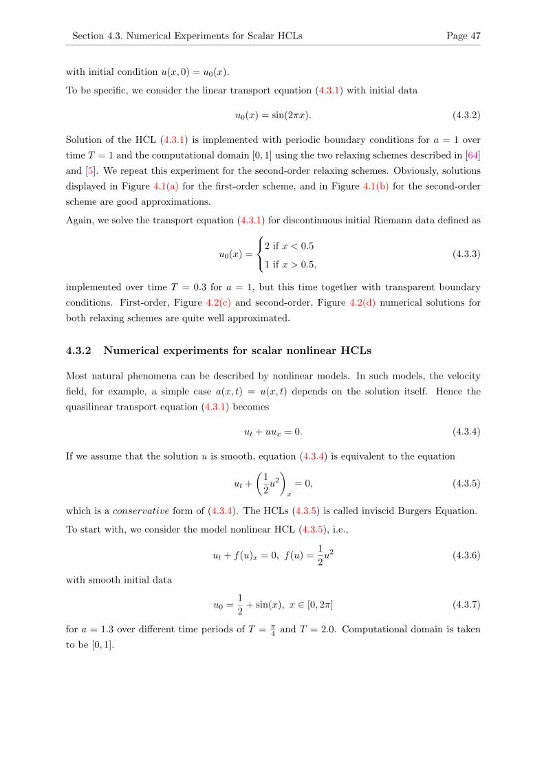
Section 4.3. Numerical Experiments for Scalar HCLs Page 47
with initial condition u(x, 0) = u0(x).
To be specific, we consider the linear transport equation (4.3.1) with initial data
u0(x) = sin(2πx). (4.3.2)
Solution of the HCL (4.3.1) is implemented with periodic boundary conditions for a = 1 over
time T = 1 and the computational domain [0, 1] using the two relaxing schemes described in [64]
and [5]. We repeat this experiment for the second-order relaxing schemes. Obviously, solutions
displayed in Figure 4.1(a) for the first-order scheme, and in Figure 4.1(b) for the second-order
scheme are good approximations.
Again, we solve the transport equation (4.3.1) for discontinuous initial Riemann data defined as
u0(x) =
2 if x < 0.5
1 if x > 0.5,(4.3.3)
implemented over time T = 0.3 for a = 1, but this time together with transparent boundary
conditions. First-order, Figure 4.2(c) and second-order, Figure 4.2(d) numerical solutions for
both relaxing schemes are quite well approximated.
4.3.2 Numerical experiments for scalar nonlinear HCLs
Most natural phenomena can be described by nonlinear models. In such models, the velocity
field, for example, a simple case a(x, t) = u(x, t) depends on the solution itself. Hence the
quasilinear transport equation (4.3.1) becomes
ut + uux = 0. (4.3.4)
If we assume that the solution u is smooth, equation (4.3.4) is equivalent to the equation
ut +
(1
2u2
)x
= 0, (4.3.5)
which is a conservative form of (4.3.4). The HCLs (4.3.5) is called inviscid Burgers Equation.
To start with, we consider the model nonlinear HCL (4.3.5), i.e.,
ut + f(u)x = 0, f(u) =1
2u2 (4.3.6)
with smooth initial data
u0 =1
2+ sin(x), x ∈ [0, 2π] (4.3.7)
for a = 1.3 over different time periods of T = π4 and T = 2.0. Computational domain is taken
to be [0, 1].
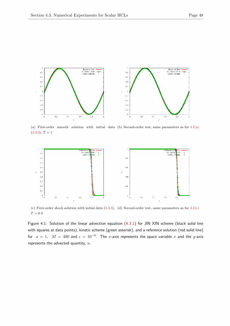
Section 4.3. Numerical Experiments for Scalar HCLs Page 48
(a) First-order smooth solution with initial data
(4.3.2), T = 1
(b) Second-order test, same parameters as for 4.1(a)
(c) First-order shock solution with initial data (4.3.3),
T = 0.3
(d) Second-order test, same parameters as for 4.1(c)
Figure 4.1: Solution of the linear advection equation (4.3.1) for JIN XIN scheme (black solid line
with squares at data points), kinetic scheme (green asterisk), and a reference solution (red solid line)
for a = 1, M = 400 and ε = 10−8. The x-axis represents the space variable x and the y-axis
represents the advected quantity, u.
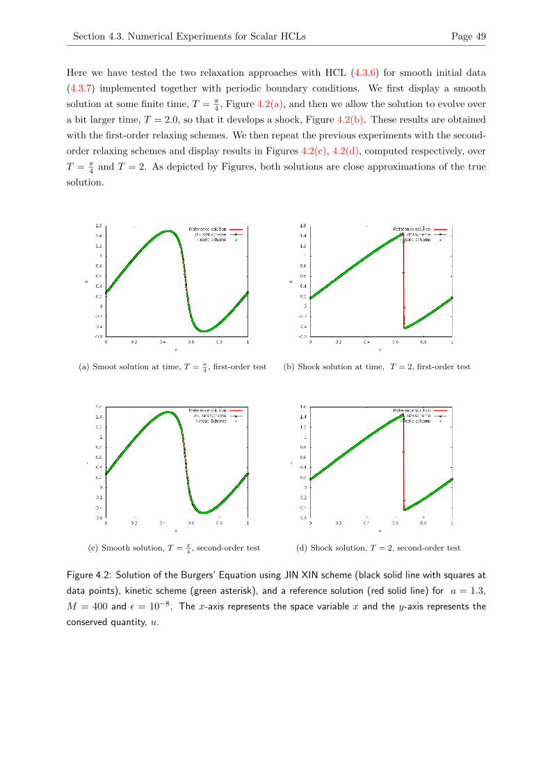
Section 4.3. Numerical Experiments for Scalar HCLs Page 49
Here we have tested the two relaxation approaches with HCL (4.3.6) for smooth initial data
(4.3.7) implemented together with periodic boundary conditions. We first display a smooth
solution at some finite time, T = π4 , Figure 4.2(a), and then we allow the solution to evolve over
a bit larger time, T = 2.0, so that it develops a shock, Figure 4.2(b). These results are obtained
with the first-order relaxing schemes. We then repeat the previous experiments with the second-
order relaxing schemes and display results in Figures 4.2(c), 4.2(d), computed respectively, over
T = π4 and T = 2. As depicted by Figures, both solutions are close approximations of the true
solution.
(a) Smoot solution at time, T = π4
, first-order test (b) Shock solution at time, T = 2, first-order test
(c) Smooth solution, T = π4
, second-order test (d) Shock solution, T = 2, second-order test
Figure 4.2: Solution of the Burgers’ Equation using JIN XIN scheme (black solid line with squares at
data points), kinetic scheme (green asterisk), and a reference solution (red solid line) for a = 1.3,
M = 400 and ε = 10−8. The x-axis represents the space variable x and the y-axis represents the
conserved quantity, u.
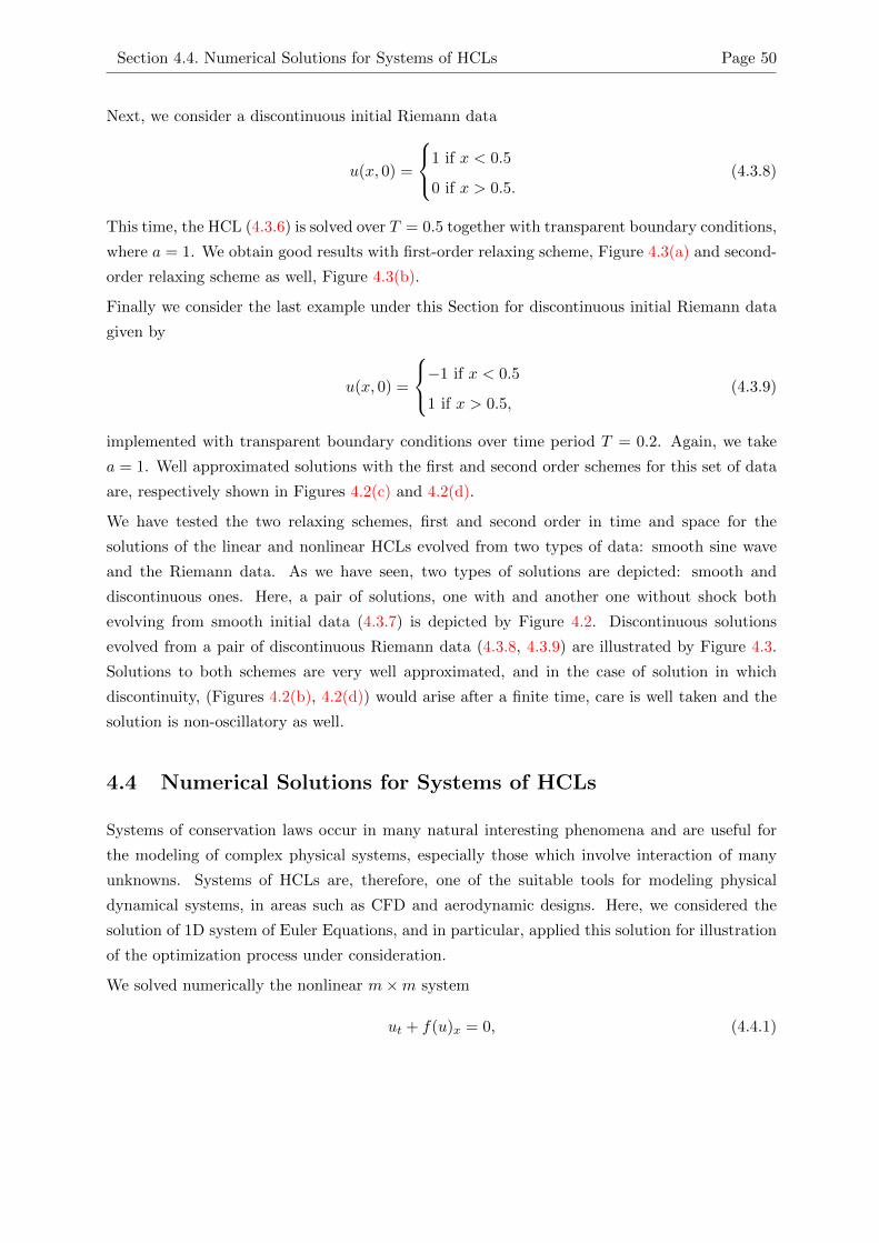
Section 4.4. Numerical Solutions for Systems of HCLs Page 50
Next, we consider a discontinuous initial Riemann data
u(x, 0) =
1 if x < 0.5
0 if x > 0.5.(4.3.8)
This time, the HCL (4.3.6) is solved over T = 0.5 together with transparent boundary conditions,
where a = 1. We obtain good results with first-order relaxing scheme, Figure 4.3(a) and second-
order relaxing scheme as well, Figure 4.3(b).
Finally we consider the last example under this Section for discontinuous initial Riemann data
given by
u(x, 0) =
−1 if x < 0.5
1 if x > 0.5,(4.3.9)
implemented with transparent boundary conditions over time period T = 0.2. Again, we take
a = 1. Well approximated solutions with the first and second order schemes for this set of data
are, respectively shown in Figures 4.2(c) and 4.2(d).
We have tested the two relaxing schemes, first and second order in time and space for the
solutions of the linear and nonlinear HCLs evolved from two types of data: smooth sine wave
and the Riemann data. As we have seen, two types of solutions are depicted: smooth and
discontinuous ones. Here, a pair of solutions, one with and another one without shock both
evolving from smooth initial data (4.3.7) is depicted by Figure 4.2. Discontinuous solutions
evolved from a pair of discontinuous Riemann data (4.3.8, 4.3.9) are illustrated by Figure 4.3.
Solutions to both schemes are very well approximated, and in the case of solution in which
discontinuity, (Figures 4.2(b), 4.2(d)) would arise after a finite time, care is well taken and the
solution is non-oscillatory as well.
4.4 Numerical Solutions for Systems of HCLs
Systems of conservation laws occur in many natural interesting phenomena and are useful for
the modeling of complex physical systems, especially those which involve interaction of many
unknowns. Systems of HCLs are, therefore, one of the suitable tools for modeling physical
dynamical systems, in areas such as CFD and aerodynamic designs. Here, we considered the
solution of 1D system of Euler Equations, and in particular, applied this solution for illustration
of the optimization process under consideration.
We solved numerically the nonlinear m×m system
ut + f(u)x = 0, (4.4.1)
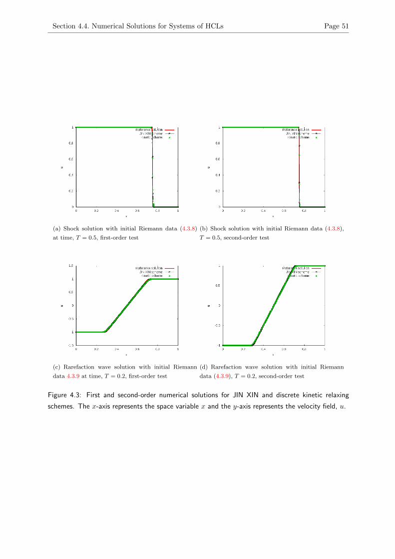
Section 4.4. Numerical Solutions for Systems of HCLs Page 51
(a) Shock solution with initial Riemann data (4.3.8)
at time, T = 0.5, first-order test
(b) Shock solution with initial Riemann data (4.3.8),
T = 0.5, second-order test
(c) Rarefaction wave solution with initial Riemann
data 4.3.9 at time, T = 0.2, first-order test
(d) Rarefaction wave solution with initial Riemann
data (4.3.9), T = 0.2, second-order test
Figure 4.3: First and second-order numerical solutions for JIN XIN and discrete kinetic relaxing
schemes. The x-axis represents the space variable x and the y-axis represents the velocity field, u.
Section 4.4. Numerical Solutions for Systems of HCLs Page 52
of HCLs in one space dimension, where
u = [u1, . . . , um]T (4.4.2)
is the vector of unknown conserved variables, and
f = [f1, . . . , fm]T (4.4.3)
is the vector of flux functions. When m = 1, the system (4.4.1) reduces to scalar HCL.
We have begun the solution of nonlinear systems of HCLs by first considering a linear system
ut +Aux = 0, (4.4.4)
which is the simplest case of (4.4.1). Specifically, we consider the one-dimensional wave equation
utt − a2uxx = 0, (x, t) ∈ (0;L)× R+, (4.4.5)
u(x, 0) = u0(x), ut(x, 0) = u1(x), x ∈ [0;L]. (4.4.6)
The wave equation (4.4.5) can be transformed into a system of first-order equations by making
change of variables v = ux, and w = −ut. With these changes, the wave equation (4.4.5) reduces
to
vt + awx = 0 (4.4.7)
wt + avx = 0, (x, t) ∈ (0;L)× R+, (4.4.8)
supplemented with initial conditions
v(x, 0) = v0(x) = 0, (4.4.9)
w(x, 0) = −1
a
∫ x
0u1(s)ds+ c, u1(x) = sin(πx), x ∈ [0;L]. (4.4.10)
We solved the system of equations (4.4.7) with boundary conditions for L = 1 (see Figure 4.4).
Accurate numerical solution solved with suitable initial and boundary conditions
u(x, 0) = 0, ut(x, 0) = 0 (4.4.11)
u(0, t) = 0; u(π, t) = 0, (4.4.12)
can be compared to analytical solution u(x, t) = 1a sin(at) sin(x).
Good approximations for both schemes are obtained for the solution of the problem discussed
above. Our intention here is that, the linear model equation provides crucial information for
generalization to nonlinear systems. Thus, we carried out tests to numerically solve these kind
of problems, especially those with propagating discontinuities.
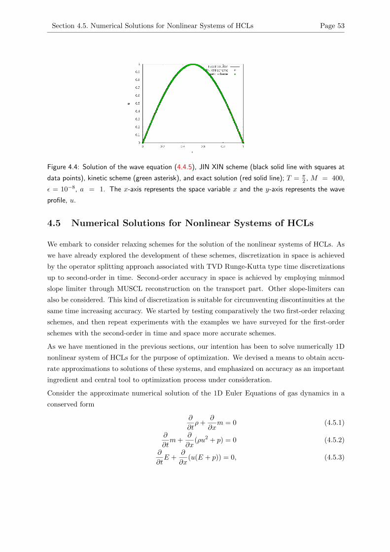
Section 4.5. Numerical Solutions for Nonlinear Systems of HCLs Page 53
Figure 4.4: Solution of the wave equation (4.4.5), JIN XIN scheme (black solid line with squares at
data points), kinetic scheme (green asterisk), and exact solution (red solid line); T = π2 , M = 400,
ε = 10−8, a = 1. The x-axis represents the space variable x and the y-axis represents the wave
profile, u.
4.5 Numerical Solutions for Nonlinear Systems of HCLs
We embark to consider relaxing schemes for the solution of the nonlinear systems of HCLs. As
we have already explored the development of these schemes, discretization in space is achieved
by the operator splitting approach associated with TVD Runge-Kutta type time discretizations
up to second-order in time. Second-order accuracy in space is achieved by employing minmod
slope limiter through MUSCL reconstruction on the transport part. Other slope-limiters can
also be considered. This kind of discretization is suitable for circumventing discontinuities at the
same time increasing accuracy. We started by testing comparatively the two first-order relaxing
schemes, and then repeat experiments with the examples we have surveyed for the first-order
schemes with the second-order in time and space more accurate schemes.
As we have mentioned in the previous sections, our intention has been to solve numerically 1D
nonlinear system of HCLs for the purpose of optimization. We devised a means to obtain accu-
rate approximations to solutions of these systems, and emphasized on accuracy as an important
ingredient and central tool to optimization process under consideration.
Consider the approximate numerical solution of the 1D Euler Equations of gas dynamics in a
conserved form
∂
∂tρ+
∂
∂xm = 0 (4.5.1)
∂
∂tm+
∂
∂x(ρu2 + p) = 0 (4.5.2)
∂
∂tE +
∂
∂x(u(E + p)) = 0, (4.5.3)
Section 4.5. Numerical Solutions for Nonlinear Systems of HCLs Page 54
where ρ, u, m = ρu, p, and E are, respectively, the density, velocity, momentun, pressure and
total energy of the gas. For a perfect gas, E is related to other quantities by
E =p
γ − 1+
1
2ρu2 (4.5.4)
where γ constitutes the thermodaynamic property of the gas and is the rato of specific heat
coefficients.
The system (4.5.1) takes the form
ut + f(u)x = 0, (4.5.5)
when we write
u =
ρ
m
E
, f(u) =
m
ρu2 + p
u(E + p)
. (4.5.6)
The relaxation system for (4.5.5) takes the form∂u∂t + ∂v
∂x = 0,
∂v∂t +A∂u
∂x = −1ε (v − f(u)),
(4.5.7)
where A = diagai, ai > 0, for 1 ≤ i ≤ 3,
and its equivalent discrete kinetic relaxation takes the form (3.5.1).
Mathematical analysis [34, 125] shows that, the relaxation (4.5.7) of the Euler equation (4.5.5)
can be decomposed as A = P ∧ P−1 where
∧ =
u− a 0 0
0 u 0
0 0 u+ a
, (4.5.8)
P =
1 1 1
u− a u u+ a
H − au 12u
2 H + au
, (4.5.9)
and
P−1 =
12(α1 + u
a ) −12(α2u+ 1
a) α22
1− α1 α2u −α2
12(α1 − u
a ) −12(α2u− 1
a) α22
(4.5.10)
Section 4.5. Numerical Solutions for Nonlinear Systems of HCLs Page 55
such that α1 = (γ−1)u2
2a2and α2 = γ−1
a2. Here a =
√γ pρ =
√γRT is the local sound speed, H is
the Enthalpy, R the universal gas constant and T is the temperature of the gas.
The relaxation system (4.5.7) therefore has three eigenvalues given by
λ− = u− a, λ0 = u, λ+ = u+ a. (4.5.11)
For computational tests, we can make the choices according to [64], i.e., a1, a2, a3 = sup|u− a|,sup|u|, sup|u + a|, respectively, or a1 = a2 = a3 = max(sup|u − a|, sup|u|, sup|u + a|), where
sup is an abbreviation for supremum, and supremum is defined as the least upper bound value
of a given set. We then solved the two relaxation systems (4.5.7) and (3.5.1) for the parameters
of our choice.
4.5.1 Sod Shock Tube Problem
Our computational tests involved experimentation with the Sod’s data for the Shock Tube
problem. To be able to understand the idea behind the shock tube we had to consider a long
1D tube which is closed at its ends and initially filled with a gas separated by a membrane at
the middle. The gas has a high pressure and density in one section of the tube than the other,
Figure 4.5. The velocity of the gas is initially zero everywhere. When the membrane is suddenly
removed at time t = 0, causes the high speed flow of the gas from high to low pressure region,
Figure 4.6. Assumming that the net flow is uniform across the tube, there will be variation in
only one direction, and this variation can be described or modeled by 1D Euler Equations of
gas dynamics considered. Detailed descriptions of the shock tube problem is found in [59, 76].
4.5.2 First and second order numerical tests
We implemented schemes we derived under Chapter 3 with the Riemann data defined in this
way: uL = (ρL, vL, pL) corresponds, respectively, to the density, velocity and pressure on the
left part of the domain for 0 ≤ x < 0.5; and uR = (ρR, vR, pR) is the data corresponding
to density, velocity and pressure on the right part of the domain for 0.5 ≤ x ≤ 1. All (unless
stated otherwise) tests for the system of the Euler equations are carried for the following set of
values: T = 0.17, the computational spatial domain [0, 1], M = 400 grid points, CFL (Courant-
Friedrichs-Lewy) = 0.75 and ε = 10−8. In addition, for the second-order relaxing schemes we
used minmod slope limiter.
We have begun the solution of the Euler equations for the following pair of Riemann data:
uL = (1.25, 0.0, 1.2), uR = (0.25, 0.0, 0.25). We take a1 = 1.0, a2 = 2.5, a3 = 5.2. Results
obtained with the first and second order relaxing schemes presented in Figure 4.7 show that the
two schemes well agree to each other.
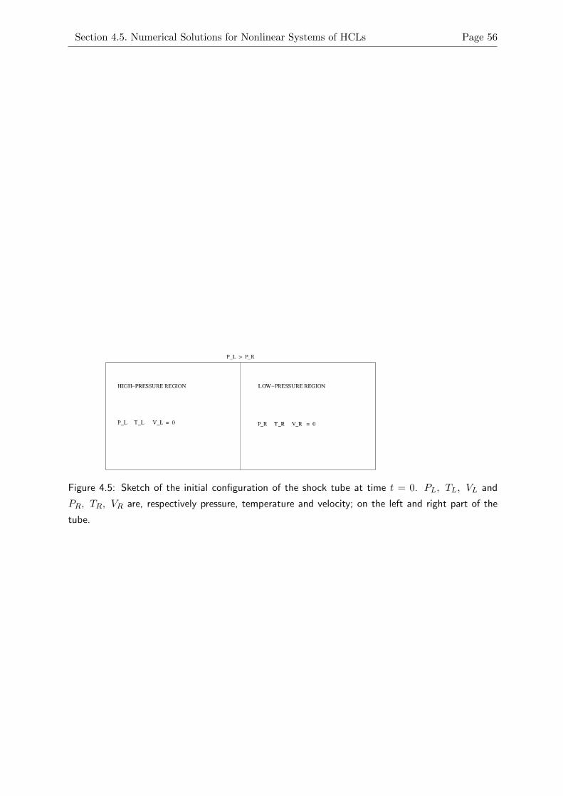
Section 4.5. Numerical Solutions for Nonlinear Systems of HCLs Page 56
Figure 4.5: Sketch of the initial configuration of the shock tube at time t = 0. PL, TL, VL and
PR, TR, VR are, respectively pressure, temperature and velocity; on the left and right part of the
tube.
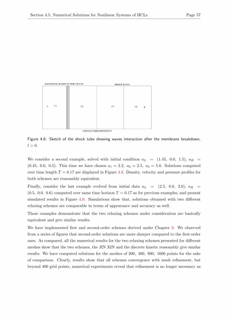
Section 4.5. Numerical Solutions for Nonlinear Systems of HCLs Page 57
Figure 4.6: Sketch of the shock tube showing waves interaction after the membrane breakdown,
t > 0.
We consider a second example, solved with initial condition uL = (1.45, 0.0, 1.5), uR =
(0.45, 0.0, 0.5). This time we have chosen a1 = 2.2, a2 = 2.5, a3 = 5.0. Solutions computed
over time length T = 0.17 are displayed in Figure 4.8. Density, velocity and pressure profiles for
both schemes are reasonably equivalent.
Finally, consider the last example evolved from initial data uL = (2.5, 0.0, 2.0), uR =
(0.5, 0.0, 0.6) computed over same time horizon T = 0.17 as for previous examples, and present
simulated results in Figure 4.9. Simulations show that, solutions obtained with two different
relaxing schemes are comparable in terms of appearance and accuracy as well.
These examples demonstrate that the two relaxing schemes under consideration are basically
equivalent and give similar results.
We have implemented first and second-order schemes derived under Chapter 3. We observed
from a series of figures that second-order solutions are more sharper compared to the first-order
ones. As compared, all the numerical results for the two relaxing schemes presented for different
meshes show that the two schemes, the JIN XIN and the discrete kinetic reasonably give similar
results. We have computed solutions for the meshes of 200, 400, 800, 1600 points for the sake
of comparison. Clearly, results show that all schemes convergence with mesh refinement, but
beyond 400 grid points, numerical experiments reveal that refinement is no longer necessary as
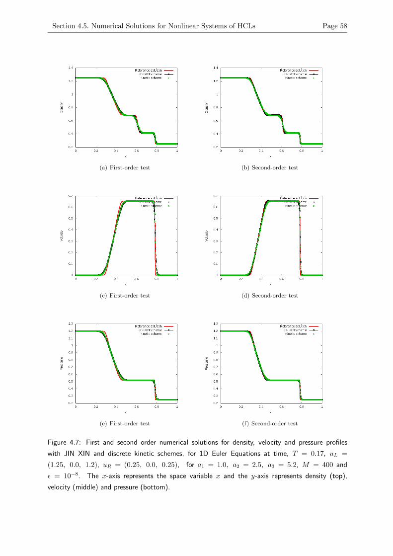
Section 4.5. Numerical Solutions for Nonlinear Systems of HCLs Page 58
(a) First-order test (b) Second-order test
(c) First-order test (d) Second-order test
(e) First-order test (f) Second-order test
Figure 4.7: First and second order numerical solutions for density, velocity and pressure profiles
with JIN XIN and discrete kinetic schemes, for 1D Euler Equations at time, T = 0.17, uL =
(1.25, 0.0, 1.2), uR = (0.25, 0.0, 0.25), for a1 = 1.0, a2 = 2.5, a3 = 5.2, M = 400 and
ε = 10−8. The x-axis represents the space variable x and the y-axis represents density (top),
velocity (middle) and pressure (bottom).
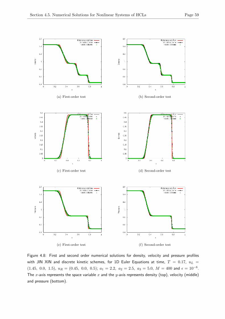
Section 4.5. Numerical Solutions for Nonlinear Systems of HCLs Page 59
(a) First-order test (b) Second-order test
(c) First-order test (d) Second-order test
(e) First-order test (f) Second-order test
Figure 4.8: First and second order numerical solutions for density, velocity and pressure profiles
with JIN XIN and discrete kinetic schemes, for 1D Euler Equations at time, T = 0.17, uL =
(1.45, 0.0, 1.5), uR = (0.45, 0.0, 0.5); a1 = 2.2, a2 = 2.5, a3 = 5.0, M = 400 and ε = 10−8.
The x-axis represents the space variable x and the y-axis represents density (top), velocity (middle)
and pressure (bottom).
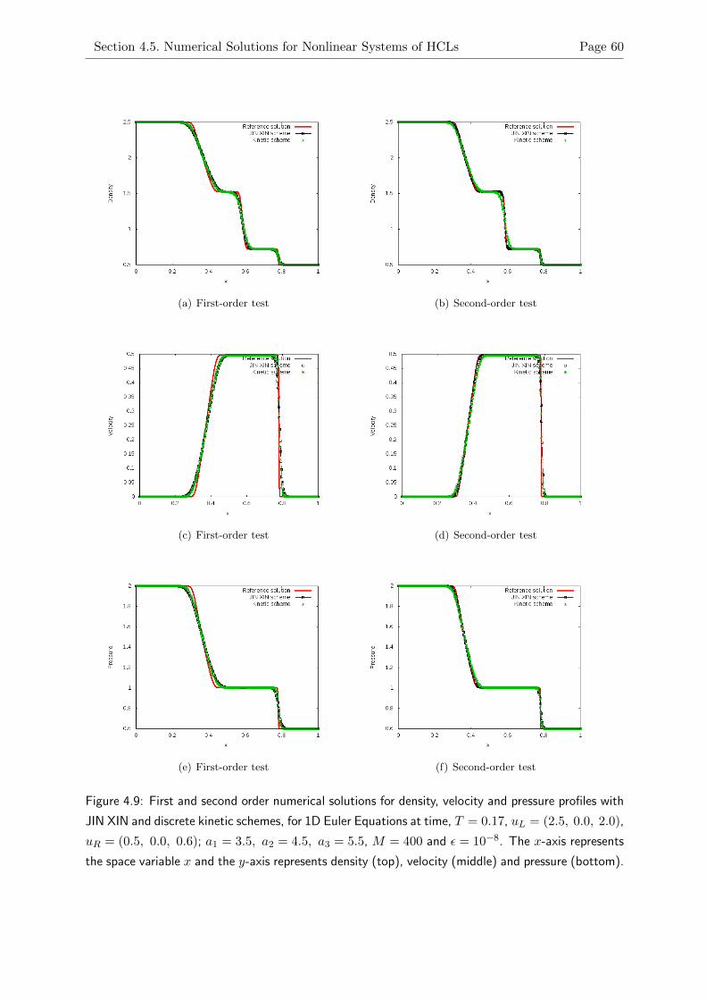
Section 4.5. Numerical Solutions for Nonlinear Systems of HCLs Page 60
(a) First-order test (b) Second-order test
(c) First-order test (d) Second-order test
(e) First-order test (f) Second-order test
Figure 4.9: First and second order numerical solutions for density, velocity and pressure profiles with
JIN XIN and discrete kinetic schemes, for 1D Euler Equations at time, T = 0.17, uL = (2.5, 0.0, 2.0),
uR = (0.5, 0.0, 0.6); a1 = 3.5, a2 = 4.5, a3 = 5.5, M = 400 and ε = 10−8. The x-axis represents
the space variable x and the y-axis represents density (top), velocity (middle) and pressure (bottom).
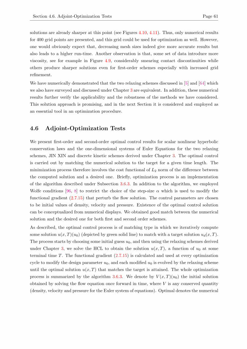
Section 4.6. Adjoint-Optimization Tests Page 61
solutions are already sharper at this point (see Figures 4.10, 4.11). Thus, only numerical results
for 400 grid points are presented, and this grid could be used for optimization as well. However,
one would obviously expect that, decreasing mesh sizes indeed give more accurate results but
also leads to a higher run-time. Another observation is that, some set of data introduce more
viscosity, see for example in Figure 4.9, considerably smearing contact discontinuities while
others produce sharper solutions even for first-order schemes especially with increased grid
refinement.
We have numerically demonstrated that the two relaxing schemes discussed in [5] and [64] which
we also have surveyed and discussed under Chapter 3 are equivalent. In addition, these numerical
results further verify the applicability and the robustness of the methods we have considered.
This solution approach is promising, and in the next Section it is considered and employed as
an essential tool in an optimization procedure.
4.6 Adjoint-Optimization Tests
We present first-order and second-order optimal control results for scalar nonlinear hyperbolic
conservation laws and the one-dimensional systems of Euler Equations for the two relaxing
schemes, JIN XIN and discrete kinetic schemes derived under Chapter 3. The optimal control
is carried out by matching the numerical solution to the target for a given time length. The
minimization process therefore involves the cost functional of L2 norm of the difference between
the computed solution and a desired one. Briefly, optimization process is an implementation
of the algorithm described under Subsection 3.6.3. In addition to the algorithm, we employed
Wolfe conditions [96, 8] to restrict the choice of the step-size α which is used to modify the
functional gradient (2.7.15) that perturb the flow solution. The control parameters are chosen
to be initial values of density, velocity and pressure. Existence of the optimal control solution
can be conceptualized from numerical displays. We obtained good match between the numerical
solution and the desired one for both first and second order schemes.
As described, the optimal control process is of matching type in which we iteratively compute
some solution u(x, T )(u0) (depicted by green solid line) to match with a target solution ud(x, T ).
The process starts by choosing some initial guess u0, and then using the relaxing schemes derived
under Chapter 3, we solve the HCL to obtain the solution u(x, T ), a function of u0 at some
terminal time T . The functional gradient (2.7.15) is calculated and used at every optimization
cycle to modify the design parameter u0, and each modified u0 is evolved by the relaxing scheme
until the optimal solution u(x, T ) that matches the target is attained. The whole optimization
process is summarized by the algorithm 3.6.3. We denote by V (x, T )(u0) the initial solution
obtained by solving the flow equation once forward in time, where V is any conserved quantity
(density, velocity and pressure for the Euler system of equations). Optimal denotes the numerical
Section 4.6. Adjoint-Optimization Tests Page 62
(a) First-order (b) Second-order
(c) First-order (d) Second-order
(e) First-order (f) Second-order
Figure 4.10: Comparing first-order and second-order solutions for different grids with JIN XIN scheme;
T = 0.17, uL = (2.5, 0.0, 2.0), uR = (0.5, 0.0, 0.6); a1 = 2.0, a2 = 3.5, a3 = 5.5, ε = 10−8.
The x-axis represents the space variable x and the y-axis represents density (top), velocity (middle)
and pressure (bottom).
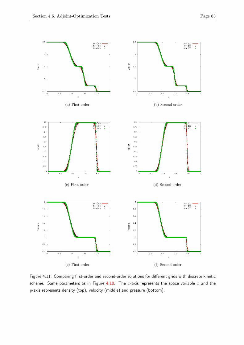
Section 4.6. Adjoint-Optimization Tests Page 63
(a) First-order (b) Second-order
(c) First-order (d) Second-order
(e) First-order (f) Second-order
Figure 4.11: Comparing first-order and second-order solutions for different grids with discrete kinetic
scheme. Same parameters as in Figure 4.10. The x-axis represents the space variable x and the
y-axis represents density (top), velocity (middle) and pressure (bottom).
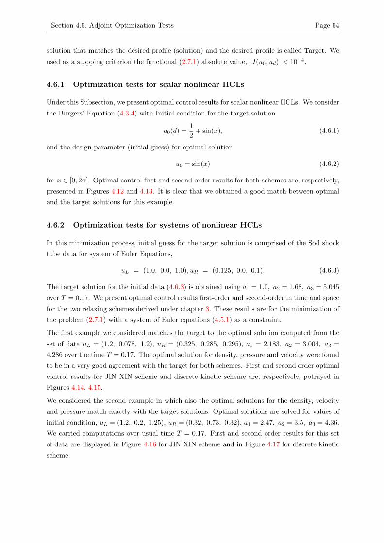
Section 4.6. Adjoint-Optimization Tests Page 64
solution that matches the desired profile (solution) and the desired profile is called Target. We
used as a stopping criterion the functional (2.7.1) absolute value, |J(u0, ud)| < 10−4.
4.6.1 Optimization tests for scalar nonlinear HCLs
Under this Subsection, we present optimal control results for scalar nonlinear HCLs. We consider
the Burgers’ Equation (4.3.4) with Initial condition for the target solution
u0(d) =1
2+ sin(x), (4.6.1)
and the design parameter (initial guess) for optimal solution
u0 = sin(x) (4.6.2)
for x ∈ [0, 2π]. Optimal control first and second order results for both schemes are, respectively,
presented in Figures 4.12 and 4.13. It is clear that we obtained a good match between optimal
and the target solutions for this example.
4.6.2 Optimization tests for systems of nonlinear HCLs
In this minimization process, initial guess for the target solution is comprised of the Sod shock
tube data for system of Euler Equations,
uL = (1.0, 0.0, 1.0), uR = (0.125, 0.0, 0.1). (4.6.3)
The target solution for the initial data (4.6.3) is obtained using a1 = 1.0, a2 = 1.68, a3 = 5.045
over T = 0.17. We present optimal control results first-order and second-order in time and space
for the two relaxing schemes derived under chapter 3. These results are for the minimization of
the problem (2.7.1) with a system of Euler equations (4.5.1) as a constraint.
The first example we considered matches the target to the optimal solution computed from the
set of data uL = (1.2, 0.078, 1.2), uR = (0.325, 0.285, 0.295), a1 = 2.183, a2 = 3.004, a3 =
4.286 over the time T = 0.17. The optimal solution for density, pressure and velocity were found
to be in a very good agreement with the target for both schemes. First and second order optimal
control results for JIN XIN scheme and discrete kinetic scheme are, respectively, potrayed in
Figures 4.14, 4.15.
We considered the second example in which also the optimal solutions for the density, velocity
and pressure match exactly with the target solutions. Optimal solutions are solved for values of
initial condition, uL = (1.2, 0.2, 1.25), uR = (0.32, 0.73, 0.32), a1 = 2.47, a2 = 3.5, a3 = 4.36.
We carried computations over usual time T = 0.17. First and second order results for this set
of data are displayed in Figure 4.16 for JIN XIN scheme and in Figure 4.17 for discrete kinetic
scheme.
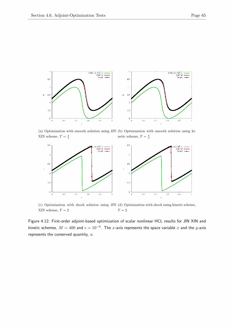
Section 4.6. Adjoint-Optimization Tests Page 65
(a) Optimization with smooth solution using JIN
XIN scheme, T = π4
(b) Optimization with smooth solution using ki-
netic scheme, T = π4
(c) Optimization with shock solution using JIN
XIN scheme, T = 2
(d) Optimization with shock using kinetic scheme,
T = 2
Figure 4.12: First-order adjoint-based optimization of scalar nonlinear HCL results for JIN XIN and
kinetic schemes, M = 400 and ε = 10−8. The x-axis represents the space variable x and the y-axis
represents the conserved quantity, u.
Section 4.6. Adjoint-Optimization Tests Page 66
(a) Optimization with smooth solution using JIN
XIN scheme, T = π4
(b) Optimization with smooth solution using ki-
netic scheme, T = π4
(c) Optimization with shock solution using JIN
XIN scheme, T = 2
(d) Optimization with shock using kinetic scheme,
T = 2
Figure 4.13: Same parameters as in Figure 4.12 but second-order tests. The x-axis represents the
space variable x and the y-axis represents the conserved quantity, u.
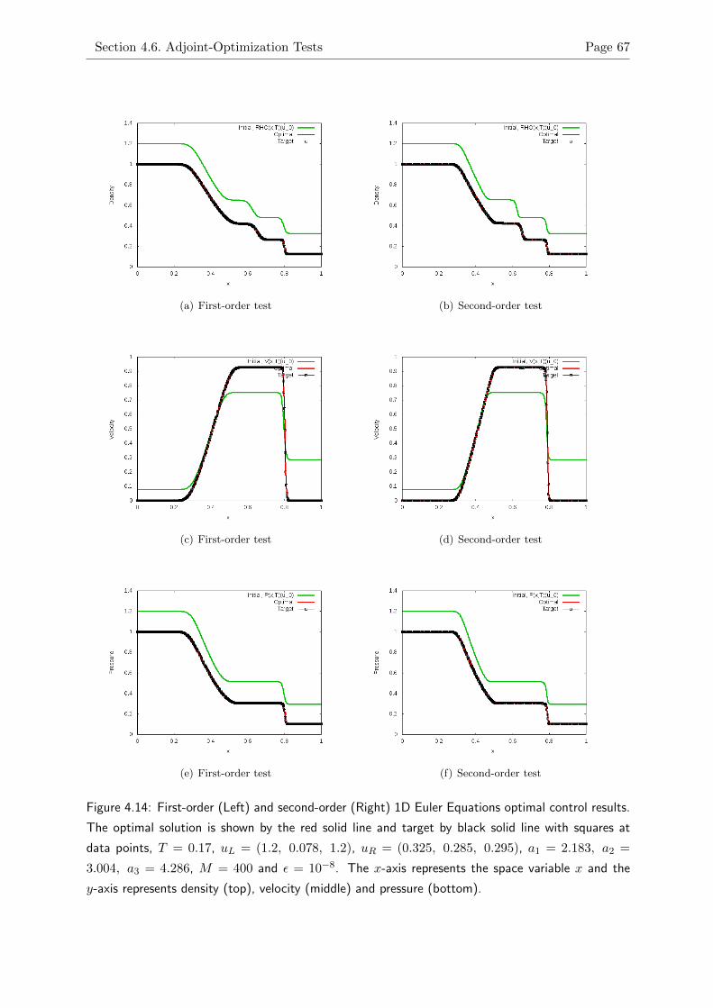
Section 4.6. Adjoint-Optimization Tests Page 67
(a) First-order test (b) Second-order test
(c) First-order test (d) Second-order test
(e) First-order test (f) Second-order test
Figure 4.14: First-order (Left) and second-order (Right) 1D Euler Equations optimal control results.
The optimal solution is shown by the red solid line and target by black solid line with squares at
data points, T = 0.17, uL = (1.2, 0.078, 1.2), uR = (0.325, 0.285, 0.295), a1 = 2.183, a2 =
3.004, a3 = 4.286, M = 400 and ε = 10−8. The x-axis represents the space variable x and the
y-axis represents density (top), velocity (middle) and pressure (bottom).
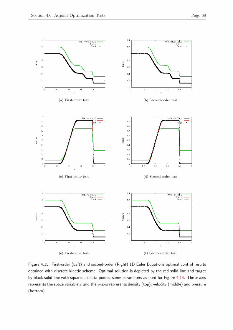
Section 4.6. Adjoint-Optimization Tests Page 68
(a) First-order test (b) Second-order test
(c) First-order test (d) Second-order test
(e) First-order test (f) Second-order test
Figure 4.15: First-order (Left) and second-order (Right) 1D Euler Equations optimal control results
obtained with discrete kinetic scheme. Optimal solution is depicted by the red solid line and target
by black solid line with squares at data points, same parameters as used for Figure 4.14. The x-axis
represents the space variable x and the y-axis represents density (top), velocity (middle) and pressure
(bottom).
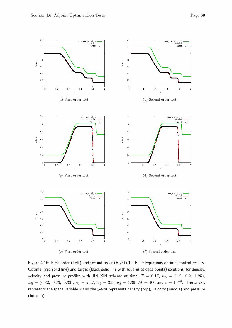
Section 4.6. Adjoint-Optimization Tests Page 69
(a) First-order test (b) Second-order test
(c) First-order test (d) Second-order test
(e) First-order test (f) Second-order test
Figure 4.16: First-order (Left) and second-order (Right) 1D Euler Equations optimal control results.
Optimal (red solid line) and target (black solid line with squares at data points) solutions, for density,
velocity and pressure profiles with JIN XIN scheme at time, T = 0.17, uL = (1.2, 0.2, 1.25),
uR = (0.32, 0.73, 0.32), a1 = 2.47, a2 = 3.5, a3 = 4.36, M = 400 and ε = 10−8. The x-axis
represents the space variable x and the y-axis represents density (top), velocity (middle) and pressure
(bottom).
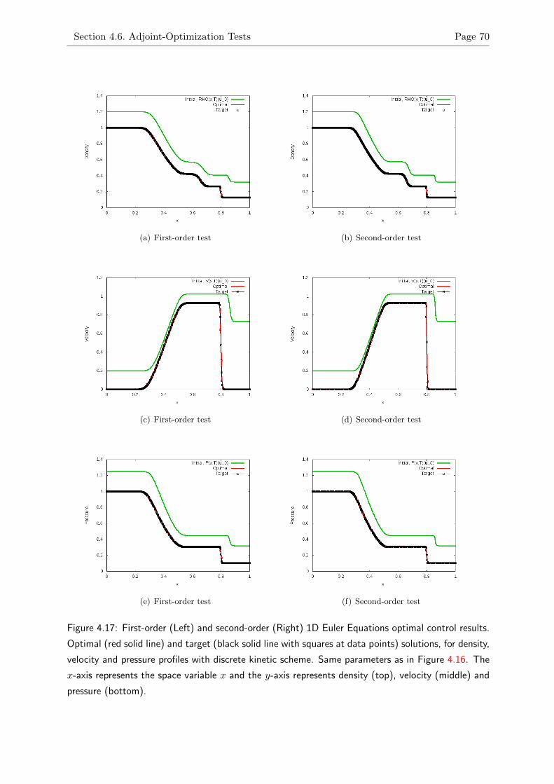
Section 4.6. Adjoint-Optimization Tests Page 70
(a) First-order test (b) Second-order test
(c) First-order test (d) Second-order test
(e) First-order test (f) Second-order test
Figure 4.17: First-order (Left) and second-order (Right) 1D Euler Equations optimal control results.
Optimal (red solid line) and target (black solid line with squares at data points) solutions, for density,
velocity and pressure profiles with discrete kinetic scheme. Same parameters as in Figure 4.16. The
x-axis represents the space variable x and the y-axis represents density (top), velocity (middle) and
pressure (bottom).
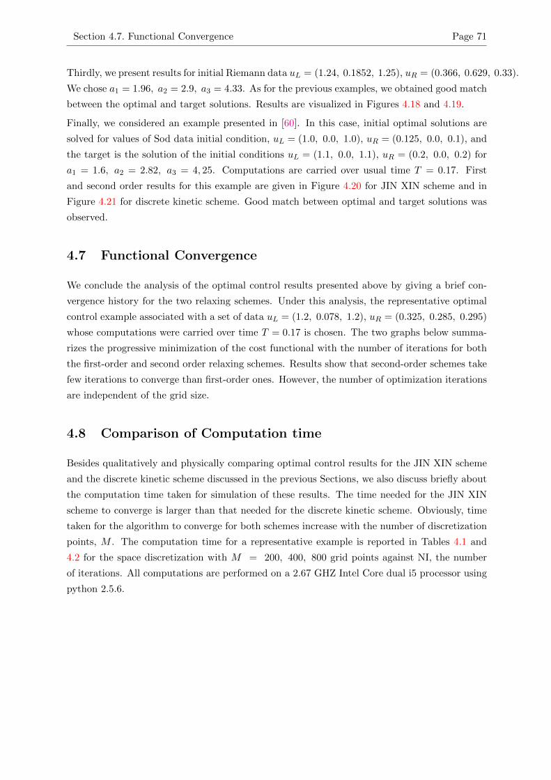
Section 4.7. Functional Convergence Page 71
Thirdly, we present results for initial Riemann data uL = (1.24, 0.1852, 1.25), uR = (0.366, 0.629, 0.33).
We chose a1 = 1.96, a2 = 2.9, a3 = 4.33. As for the previous examples, we obtained good match
between the optimal and target solutions. Results are visualized in Figures 4.18 and 4.19.
Finally, we considered an example presented in [60]. In this case, initial optimal solutions are
solved for values of Sod data initial condition, uL = (1.0, 0.0, 1.0), uR = (0.125, 0.0, 0.1), and
the target is the solution of the initial conditions uL = (1.1, 0.0, 1.1), uR = (0.2, 0.0, 0.2) for
a1 = 1.6, a2 = 2.82, a3 = 4, 25. Computations are carried over usual time T = 0.17. First
and second order results for this example are given in Figure 4.20 for JIN XIN scheme and in
Figure 4.21 for discrete kinetic scheme. Good match between optimal and target solutions was
observed.
4.7 Functional Convergence
We conclude the analysis of the optimal control results presented above by giving a brief con-
vergence history for the two relaxing schemes. Under this analysis, the representative optimal
control example associated with a set of data uL = (1.2, 0.078, 1.2), uR = (0.325, 0.285, 0.295)
whose computations were carried over time T = 0.17 is chosen. The two graphs below summa-
rizes the progressive minimization of the cost functional with the number of iterations for both
the first-order and second order relaxing schemes. Results show that second-order schemes take
few iterations to converge than first-order ones. However, the number of optimization iterations
are independent of the grid size.
4.8 Comparison of Computation time
Besides qualitatively and physically comparing optimal control results for the JIN XIN scheme
and the discrete kinetic scheme discussed in the previous Sections, we also discuss briefly about
the computation time taken for simulation of these results. The time needed for the JIN XIN
scheme to converge is larger than that needed for the discrete kinetic scheme. Obviously, time
taken for the algorithm to converge for both schemes increase with the number of discretization
points, M . The computation time for a representative example is reported in Tables 4.1 and
4.2 for the space discretization with M = 200, 400, 800 grid points against NI, the number
of iterations. All computations are performed on a 2.67 GHZ Intel Core dual i5 processor using
python 2.5.6.
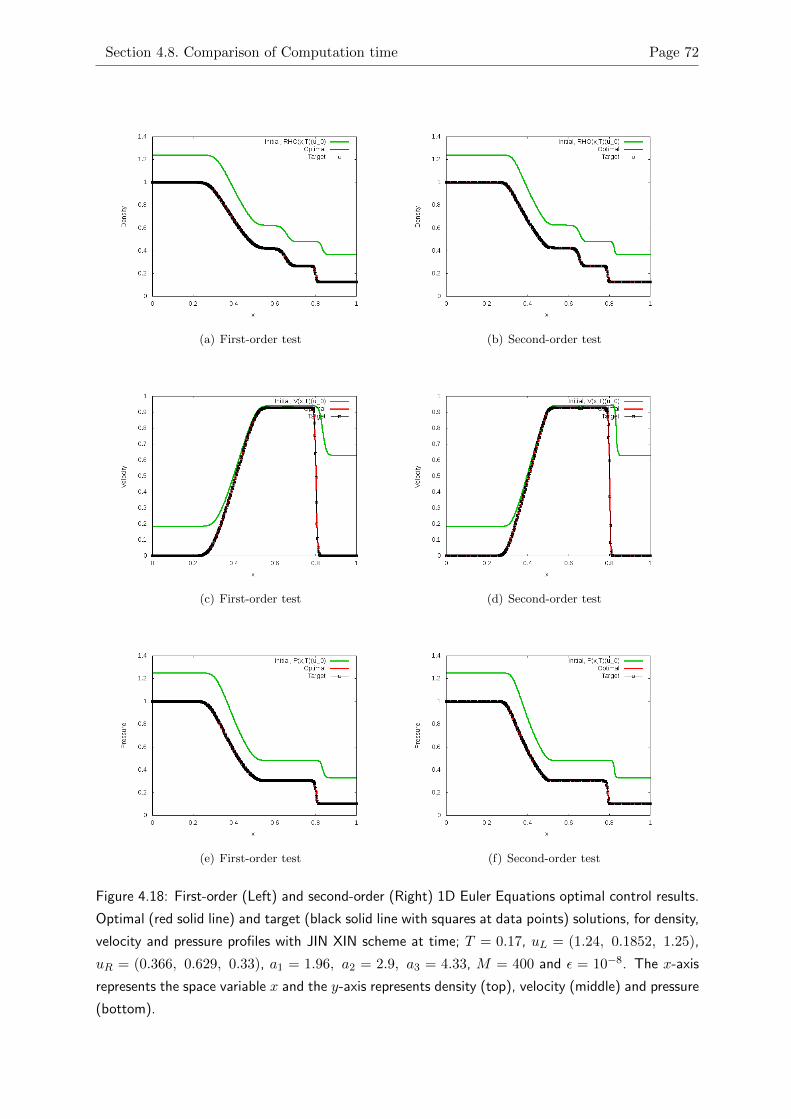
Section 4.8. Comparison of Computation time Page 72
(a) First-order test (b) Second-order test
(c) First-order test (d) Second-order test
(e) First-order test (f) Second-order test
Figure 4.18: First-order (Left) and second-order (Right) 1D Euler Equations optimal control results.
Optimal (red solid line) and target (black solid line with squares at data points) solutions, for density,
velocity and pressure profiles with JIN XIN scheme at time; T = 0.17, uL = (1.24, 0.1852, 1.25),
uR = (0.366, 0.629, 0.33), a1 = 1.96, a2 = 2.9, a3 = 4.33, M = 400 and ε = 10−8. The x-axis
represents the space variable x and the y-axis represents density (top), velocity (middle) and pressure
(bottom).
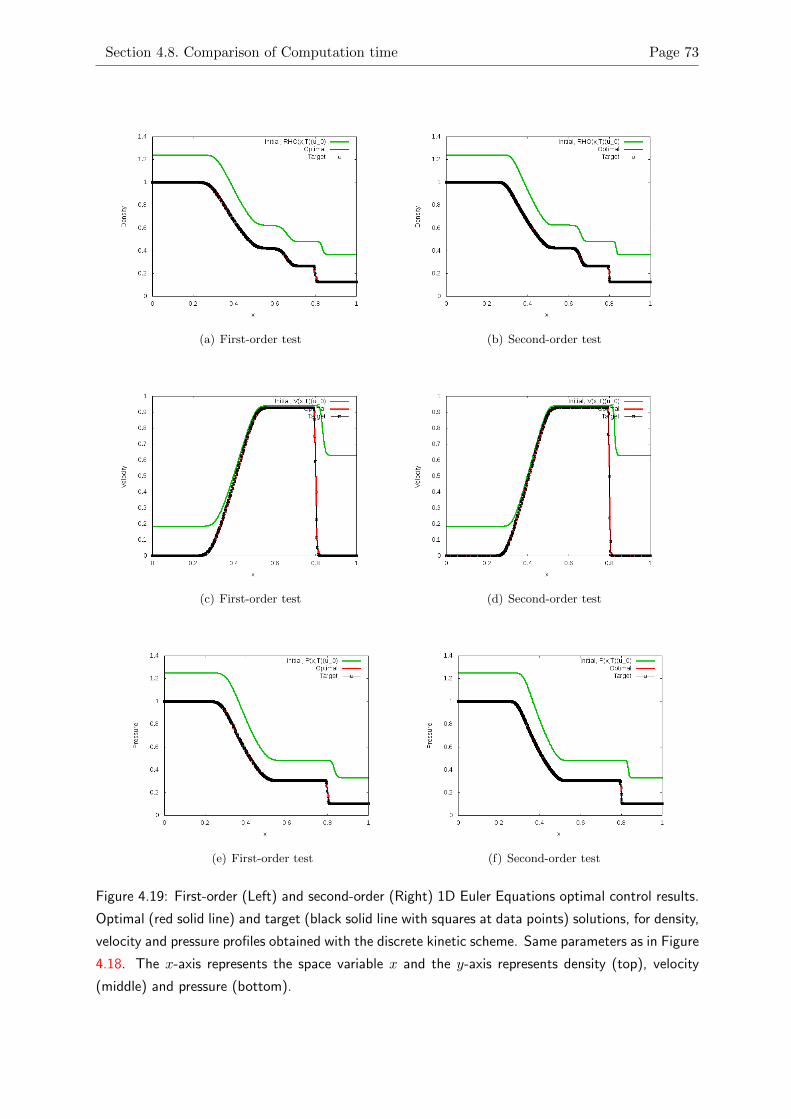
Section 4.8. Comparison of Computation time Page 73
(a) First-order test (b) Second-order test
(c) First-order test (d) Second-order test
(e) First-order test (f) Second-order test
Figure 4.19: First-order (Left) and second-order (Right) 1D Euler Equations optimal control results.
Optimal (red solid line) and target (black solid line with squares at data points) solutions, for density,
velocity and pressure profiles obtained with the discrete kinetic scheme. Same parameters as in Figure
4.18. The x-axis represents the space variable x and the y-axis represents density (top), velocity
(middle) and pressure (bottom).
Section 4.8. Comparison of Computation time Page 74
(a) First-order test (b) Second-order test
(c) First-order test (d) Second-order test
(e) First-order test (f) Second-order test
Figure 4.20: First-order (Left) and second-order (Right) 1D Euler Equations optimal control results.
Optimal (red solid line) and target (black solid line with squares at data points) solutions, for
density, velocity and pressure profiles with JIN XIN scheme at time, T = 0.17, uL = (1.0, 0.0, 1.0),
uR = (0.1, 0.0, 0.125) for optimal; and uL = (1.1, 0.0, 1.1), uR = (0.2, 0.0, 0.2) for target.
a1 = 1.96, a2 = 2.9, a3 = 4.33, M = 400 and ε = 10−8. The x-axis represents the space variable
x and the y-axis represents density (top), velocity (middle) and pressure (bottom).
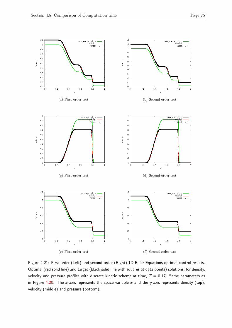
Section 4.8. Comparison of Computation time Page 75
(a) First-order test (b) Second-order test
(c) First-order test (d) Second-order test
(e) First-order test (f) Second-order test
Figure 4.21: First-order (Left) and second-order (Right) 1D Euler Equations optimal control results.
Optimal (red solid line) and target (black solid line with squares at data points) solutions, for density,
velocity and pressure profiles with discrete kinetic scheme at time, T = 0.17. Same parameters as
in Figure 4.20. The x-axis represents the space variable x and the y-axis represents density (top),
velocity (middle) and pressure (bottom).
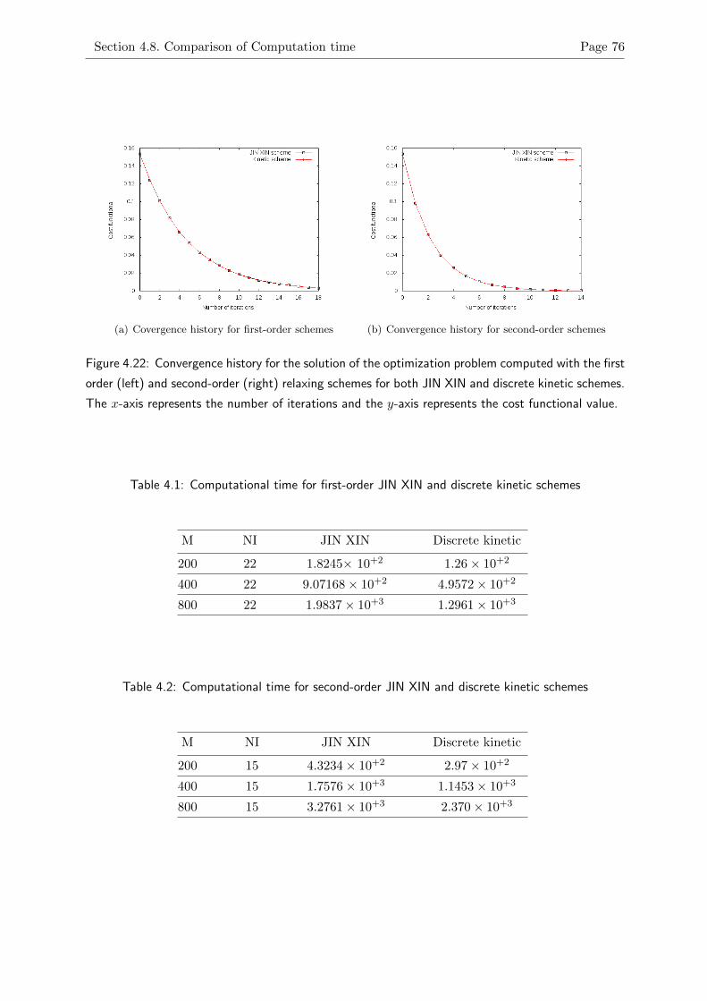
Section 4.8. Comparison of Computation time Page 76
(a) Covergence history for first-order schemes (b) Convergence history for second-order schemes
Figure 4.22: Convergence history for the solution of the optimization problem computed with the first
order (left) and second-order (right) relaxing schemes for both JIN XIN and discrete kinetic schemes.
The x-axis represents the number of iterations and the y-axis represents the cost functional value.
Table 4.1: Computational time for first-order JIN XIN and discrete kinetic schemes
M NI JIN XIN Discrete kinetic
200 22 1.8245× 10+2 1.26× 10+2
400 22 9.07168× 10+2 4.9572× 10+2
800 22 1.9837× 10+3 1.2961× 10+3
Table 4.2: Computational time for second-order JIN XIN and discrete kinetic schemes
M NI JIN XIN Discrete kinetic
200 15 4.3234× 10+2 2.97× 10+2
400 15 1.7576× 10+3 1.1453× 10+3
800 15 3.2761× 10+3 2.370× 10+3
5. Conclusions
This research has been a tour on a mixed survey of well-known results and the present contribu-
tions. A great deal of theoretical perspectives from previous works has been substantiated by the
numerical results obtained, second-order adjoint-based optimization in this context. However,
a review and development of effective numerical schemes has been central to our optimization
approach.
Research has been focused on the adjoint approach to optimize problem constrained by nonlinear
systems of HCLs. We started by deriving the optimality systems for the two relaxation approach
discussed, we then developed their corresponding relaxing schemes: first and second order in
time and space. These schemes were then tested for both the solutions and the adjoint-based
optimal control of the scalar and systems of HCLs. Contrary to the existing numerical results
in [10, 94, 128], we have managed to utilize the theoretical second-order adjoint scheme derived
in [10], and obtained up to second-order optimal control numerical results. Although for the
second-order optimal control, the descent is computed via a first-order gradient method, we are
convinced that this is a reasonable estimate since all the coupling information that involve in
calculation of gradient come from the second-order schemes. However, we reviewed the first-
order optimal control numerical results discussed in [10, 94, 128], and through generalization
we were able to develop new adjoint relaxing schemes, first-order and second-order in time and
space for the discrete kinetic model. The coupling information obtained by solving flow and
adjoint systems during optimization cycle, enabled us to complete the optimization process, the
first and second order numerical results obtained are promising and comparable.
Talking from efficient point of view, computer runtimes for both schemes, of the flow equations
and that of the adjoint equations are almost equal. But the discrete kinetic scheme takes
shorter computer runtime compared to the she JIN XIN scheme. Results convince that storage
requirements are solely equal since each scheme fundamentally handles and processes almost the
same amount of data during computations. We can roughly draw that, a single optimization
cycle is equivalent to solving two to three times the flow equation. If there are extra constraints
added to the optimization algorithm in order to satisfy certain conditions, this may no longer
be the case.
Care have been taken in solving the adjoint systems as discontinuities soon develop when solving
backward in time. This realm is due to the fact that solutions for HCLs are not easily reversible
and highly unstable even for scalar conservation laws. Characteristics interact immediately
loosing the correct track of information propagation. We realized that, there must be a means
to check that stability condition is satisfied at every optimization cycle. Therefore, information
that pertains to insuring stability condition is subject to change at every step. Comparing the
two schemes for flow and adjoint equations in term of stability, adjoint scheme is more prone
77

Page 78
and suffers severely than the scheme for the flow equations.
This study has been motivated by the fact that, both the HCLs and the adjoint-based opti-
mization considered have a lot of applications in the real life. For example, transport equation
in modeling chemical processes and pollutants in a river, Burgers’ Equation could be applied
in modeling traffic flows. For systems of HCLs, we have considered the Euler Equations of gas
dynamics, typically applied in modeling gas in pipelines and in aircraft configurations. It is our
expectations that, this study could have contributions in these areas of applications and also
brings challenges to researchers and scientists for further investigations.
It was never expected that, this study could explain all, and it has not done so far. We hope
this study will be judged, not primarily by the degree to which it explains, but by the extent to
which it lays down the foundation for further work. Options for further research in the context
of this work are diverse. One may decide to extend this research to incorporate much higher-
order schemes during optimization process. It is also possible to extend this work to deal with
multi-dimensional problems, especially when bearing in mind that the approach is featured by a
number of valuable characteristics which make it easily extendable. However, adjoint approach
to optimization, as we have discussed, can be inter-twined with other numerical schemes for
optimization purpose apart from relaxing. More importantly, is to consider high than first-order
optimality conditions for adjoint-based optimization. Finally, our future work may involve one
or more of the possible extensions we have mentioned, most likely, we intend to apply similar
ideas to consider high order optimality conditions.
Bibliography
[1] D. A. ANDERSON, J. C. TANNEHILL, and R. H. PLETCHER. Computational Fluid
Mechanics and Heat Transfer. McGraw-Hill, 1984.
[2] W. K. ANDERSON and D. L. BONHAUS. Airfoil design on unstructured grids for tur-
bulent flows. AIAA J., 37(2):185–191, 1999.
[3] W. K. ANDERSON and V. VENKATAKRISHNAN. Aerodynamic design optimization
on unstructured grids with a continuous adjoint formulation. AIAA Paper 97-0643, 1997.
[4] R. ANSORGE. Towards numerical procedures for those technical phenomena whose math-
ematical models leads to non-standard conservation laws: A survey. Mathematics and
Computers in Simulation, ELSEVIER, 61:449–463, 2003.
[5] D. AREGBA-DRIOLLET and V. MILISIC. Kinetic approximation of a boundary value
problem for conservation laws. J. Num. Math., 97:595–633, 2004.
[6] D. AREGBA-DRIOLLET and R. NATALINI. Convergence of relaxation schemes for
conservation laws. Applicable Analysis, (61):163–193, 1996.
[7] D. AREGBA-DRIOLLET and R. NATALINI. Discrete kinetic schemes for multidimen-
sional conservation laws. SIAM J. Numer. Anal., 37(6):1973–2004, 2000.
[8] L. ARMIJO. Minimization of functions having Lipschitz continuous first partial deriva-
tives. Pacific J. Math, 16(1):1–3, 1966.
[9] M. K. BANDA and M. HERTY. Multiscale modeling of gas flow in pipe networks. Math-
ematical Methods in the Applied Sciences, 31(8):915–936, 2008.
[10] M. K. BANDA and M. HERTY. Adjoint IMEX-based schemes for control problems gov-
erned by hyperbolic conservation laws. Comput Optim Appl. DOI: 10.1007/s10589-010-
9362-2, pages 1–22, October 2010.
[11] M. K. BANDA, M. HERTY, and A. KLAR. Coupling conditions for gas network governed
by the isothermal Euler Equations. Networks and Heterogeneous media, 1(2):295–314, June
2006.
[12] M. K. BANDA, M. HERTY, and A. KLAR. Gas flow in pipeline networks. Networks and
Heterogeneous media, 1(1):41–56, March 2006.
[13] M. K. BANDA and M. SEAID. Higher-order relaxation schemes for hyperbolic systems
of conservation laws. J. Numer. Math., 13(3):171–196, May 2005.
79
BIBLIOGRAPHY Page 80
[14] P. BHATNAGAR, E. GROSS, and M. KROOK. A model for collision processes in gases.
I. small amplitude processes in charged and neutral one-component systems. Phys. Rev.,
94:511–525, 1954.
[15] S. BIANCHINI. On the shift differentiability of the flow generated by a hyperbolic system
of conservation laws. Discrete Contin. Dynam. Systems, 6(2):329–350, 2000.
[16] J. P. BORIS and D. L. BOOK. Flux corrected transport I, SHASTA, a fluid transport
algorithm that works. J. Comp. Phys., 11:38–69, 1973.
[17] F. BOUCHUT and T. MORALES de LUNA. Semi-discerete entropy satisfying approxi-
mate Riemann solvers. The case of the Suliciu relaxation approximation. 2009,
[18] F. BOUCHUT and F. JAMES. Differentiability with respect to initial data for a scalar
conservation law, International Series. Numer. Math. Birkhauser, 129:113–118, 1999.
[19] A. BRESSAN and G. GUERRA. Shift-differentiability of the flow generated by a conser-
vation law. volume 3, pages 35–58. Discrete Contin. Dynam. Systems, (1997).
[20] A. BRESSAN and M. LEWICKA. Shift differentials of maps in BV spaces, in Nonlinear
Theory of Generalized Functions, Vienna, 1997. Chapman and Hall/CRC Res. Notes
Math. Chapman and Hall/CRC, Boca Raton, FL, vol. 401:47–61, 1999.
[21] A. BRESSAN and A. MARSON. A maximum principle for optimally controlled systems
of conservation laws. Rend. Sem. Univ. Podova, 94:79–94, 1995.
[22] A. BRESSAN and A. MARSON. A variational calculus for discontinuous solutions to
conservation laws. Commun. Partial Differ. Equ., 20:1491–1552, 1995.
[23] A. BRESSAN and W. SHEN. Optimality conditions for solutions to hyperbolic balance
laws. Control methods in PDE-dynamical systems. Contemp. Math., 426:129–152, 2007.
[24] H. CABUK, C.H SHUNG, and V. MODI. Adjoint operator approach to shape design for
internal incompressible flow. In Pennyslvania State Univ., 3rd International Conference
on Inverse Design Concepts and Optimization in Engineering Sciences. 1991.
[25] M. CARPENTER and C. KENNEDY. Fourth-order 2N-storage Runge-Kutta schemes,
NASA TM 109112. NASA Langley Research Center, (MR 90k:65160), June 1994.
[26] J. CARRILLO, I. M. GAMBA, A. MAJORANA, and C.-W. SHU. A WENO-solver for
the transients of Boltzmann-Poisson systems for semiconductor devices: performance and
comparisons with Monte Carlo methods. J. Comput. Phys., 184:498–525, 2003.
[27] G. Q. CHEN, D. LEVERMORE, and T. P. LIU. Hyperbolic conservation laws with stiff
relaxation terms and entropy. Comm. Pure Appl. Math., 47(1994):787–830.
BIBLIOGRAPHY Page 81
[28] J. CHEN and Z. SHI. Application of a fourth-order relaxation scheme to hyperbolic
systems of conservation laws. Applicable Analysis, (61):163–193, December (2005).
[29] V. CHERUVU, R.D. NAIR, and H. M. TUFO. A spectral finite volume transport scheme
on the cubed sphere. Appl. Numer. Math., 57:1021–1032, 2007.
[30] B. COCKBURN, F. LI, and C.-W. SHU. Locally divergence-free discontinuous Galerkin
methods for the Maxwell Equations. J. Comput. Phys., 194:588–610, 2004.
[31] B. COCKBURN and C.-W. SHU. TVB Runge-Kutta local projection discontinuous
Galerkin finite element method for conservation laws II: General framework. Math. Comp.,
52(186):411–435, 1989.
[32] P. COLELLA. Glimm’s method for gas dynamics. SIAM J. Sci. Stat. Comput., (3):76–110,
1982.
[33] C. M. DAFERMOS. Hyeperbolic Conservation Laws in Continuum Physics, volume 325.
Springer, 2010.
[34] I. DANAILA, P. JOLY, S. M. KABER, and M. POSTEL. An Introduction to Scientific
Computing. Twelve Computational Projects Solved with MATLAB. Springer, 2006.
[35] R. DONAT and A. MARQUINA. Capturing shock reflections: an improved flux formula.
J. Comp. Phys., 125:42–58, 1996.
[36] B. EINFELDT. On Godunov-type methods for gas dynamics. SIAM J. Num. Anal.,
25:294–318, 1988.
[37] J. ELLIOTT. Aerodynamic optimization based on the Euler and Navier-Stokes equations
using unstructured grids. PhD Thesis, MIT, Department of Aeronautics and Astronomy,
1998.
[38] J. ELLIOTT and J. PERAIRE. Practical 3D aerodynamic design and optimization using
unstructured meshes. AIAA J., 35(9):1479–1485, 1997.
[39] B. ENGQUIST and S. OSHER. One sided difference schemes and transonic flow. Proc.
Nat. Acad. Sci. U.S.A., 77:3071–3074, 1980.
[40] B. ENGQUIST and S. OSHER. Stable and entropy satisfying approximations for transonic
flow calculations. Math. Comp., 34:45–75, 1980.
[41] B. ENGQUIST and S. OSHER. One sided difference approximations for nonlinear con-
servation laws. Math. Comp., 36:321–352, 1981.
BIBLIOGRAPHY Page 82
[42] L. C. EVANS. Partial Diffferential Equations. Volume 19. American Mathematical Society,
1997.
[43] L.-L. FENG, C.-W. SHU, and M. ZHANG. A hybrid cosmological hydrodynamic/n-body
code based on a weighted essentially nonoscillatory. 612:1–13, 2004.
[44] M. B. GILES and N. A. PIERCE. An introduction to the Adjoint Approach to design.
Flow, Turbul. Combust., 65(3-4):393–415, 2000.
[45] M. B. GILES and N. A. PIERCE. An Introduction to the Adjoint Approach to design.
Flow, Turbul. Combust., 65(3-4):393–415, 2000.
[46] E. GODLEWSKI and P.-A. RAVIART. Numerical Approximation of Hyperbolic Systems
of Conservation Laws. Springer-Verlag, New York, 1996.
[47] S. K. GODUNOV. A finite-difference method for the numerical computation of discontin-
uous solutions of the equations of fluid dynamics. Mat. Sb., (47):271–290, 1959.
[48] S. GOTILLIEB and C.-W. SHU. Total Variation Diminishing Runge-Kutta Schemes.
Mathematics of Computation, 67(221):73–86, 1996.
[49] S. GOTTLIEB, D. I. KETCHESON, and C.-W. SHU. High-order Strong Stability Pre-
serving Time Discretizations. Journal of Scientific Computing, 38(3), March 2009.
[50] S. GOTTLIEB, C.-W. SHU, and E. TADMOR. Strong stability-preserving high-order
time discretization methods. SIAM Rev., (43):89–112, 2001.
[51] M. D. GUNZBURGER. Perspectives in Flow Control and Optimization, Advances in
design and control. SIAM, PA. USA, 2003.
[52] W. W HAGER. Runge-Kutta methods in optimal control and the transformed adjoint
system. Numerische Mathematik, (87):247–282, 2000.
[53] A. HARTEN. In proceedings, International Conference on Hyperbolic Problems, Saint-
Etienne.
[54] A. HARTEN. High resolution schemes for hyperbolic conservation laws. J. Comput. Phys.,
49:357–393, 1983.
[55] A. HARTEN, B. ENGQUIST, S. OSHER, and S. CHAKRAVARTHY. Uniformly high-
order accurate essentially nonoscillatory schemes, III. J. Comput. Phys., 71:231–303, Au-
gust 1987.
[56] A. HARTEN and P. D. LAX. On a Class of High Resolution Total-Variation-Stable
Finite-Difference Schemes. SIAM J. Numer. Anal., 21(1):1–23, 1984.
BIBLIOGRAPHY Page 83
[57] A. HARTEN, P. D. LAX, and B. VAN LEER. On upstream differencing and Gudunov-type
schemes for hyperbolic conservation laws. SIAM Review, 25:35–61, 1983.
[58] A. HARTEN and S. OSHER. Unifromly high-order accurate nonoscillatory schemes, I.
SIAM J. Numer. Anal., 24:279–309, 1987.
[59] C. HIRSCH. Numerical Computation of Internal and External Flows. John Wiley and
Sons, 1988.
[60] C. HOMESCU and I. M. NAVON. Optimal control of flow with discontinuities. J. Comp.
Phys., 187:660–682, 2003.
[61] J. M. HYMAN. On robust and accurate methods for the calculation of compressible fluid
flows I. to appear.
[62] Z. JACKIEWICZA, R. RENAUT, and A. FELDSTEIN. Two-step Runge-Kutta methods.
SIAM J. Numer. Anal., 28:1165–1182, 1991.
[63] S. JIN. Runge-Kutta Methods for Hyperbolic Conservation Laws with Stiff Relaxation
Terms. 122(1):51–67, 1995.
[64] S. JIN and Z. XIN. The relaxation schemes for systems of conservation laws in arbitrary
space dimensions. Comm. Pure Appl. Math, (48):235–276, 1995.
[65] D. KRONER. Numerical Schemes for Conservation Laws. Wiley-Teubner series, 1997.
[66] E. J. KUBATKO, J. J. WESTERINK, and C. DAWSON. Semi discrete discontinu-
ous Galerkin methods and stage-exceeding-order, strong-stability-preserving Runge-Kutta
time discretizations. J. Comput. Phys., 222:832–848, 2007.
[67] P. D. LAX. Selected Papers. Volume I. Springer-Verlag, Arizona, 1968.
[68] P. D. LAX. Shock waves and entropy, in: E. M. Zarantello (Ed.), Contribututions to
Non-linear Functional Analysis. Academic Press, New York, 1971.
[69] P. D. LAX. Hyperbolic Systems of Conservation Laws and the Mathematical Theory of
Shock Waves, vol. II of Regional Conference Series in Applied Mathematics. SIAM, 1973.
[70] P. D. LAX. Hyperbolic Partial Differential Equations: Courant Lecture Notes in Mathem-
natics. AMS, New York, 2006.
[71] B. VAN LEER. Towards the ultimate conservative difference scheme I. the quest of mono-
tonicty. 18:163–168, 1973.
BIBLIOGRAPHY Page 84
[72] B. VAN LEER. Towards the ultimate conservative difference scheme IV. A new approach
to numerical convection. 23:276–299, 1977.
[73] B. VAN LEER. Towards the ultimate conservative difference scheme V. A second-order
sequel to Godunov’s method. 32:101–136, 1979.
[74] B. VAN LEER. Flux-vector splitting for the Euler equations. In E. Krause, volume 170.
Lecture Notes in Physics, Springer-Verlag, 1982.
[75] R. J. LEVEQUE. Numerical Methods for Conservation Laws. Birkhauser-Verlag, 1990.
[76] R. J. LEVEQUE. Numerical Methods for Conservation Laws. 2nd Edition. Birkhauser
Verlag, Berlin, 1992.
[77] R. J. LEVEQUE. Finite Volume Methods for Hyperbolic Problems. Cambridge Texts in
Applied Mathematics. Cambridge University Press, 2002.
[78] R. J. LEVEQUE, D. MIHALAS, E.A. DORFI, and E. MULLER. Computational Methods
for Astrophysical Fluid Flow: Swiss Society for Astrophysics and Astronomy, 27th Saas-
Fee Advanced Course Lecture Notes. Springer-Verlag, Berlin Heidelberg New York, 1997.
[79] M. J. LIGHTHILL and G. B. WHITHAM. A theory of traffic flow on long crowded roads.
Proc. R. Soc., London A, 229:317–345, 1955.
[80] M.-S. LIOU. A sequel to ausm: Ausm+. to appear. J. Comp. Phys.
[81] M.-S LIOU. and C. J. STEFFEN Jr. A new flux splitting scheme. J. Comp. Phys., 107:107,
1993.
[82] T. P. LIU. Hyperbolic conservation laws with relaxation. Comm. Math. Phys., 108:153–
175, 1987.
[83] X. LIU, S. OSHER, and T. CHAN. Weighted essentially non-oscillatory schemes. J.
Comput. Phys., 115:200–212, 1994.
[84] Z. LIU and A. SANDU. On the properties of discrete adjoints of numerical methods for
the advection equation. Int. J. for Num. Meth. in Fluids, (56):769–803, 2008.
[85] R. MAcCORMACK. Proceedings of the Second International Conference on Numerical
Methods in Fluid dynamics, Lecture Notes in Physics, (M. Holt, Ed.). 8, 1971.
[86] A. MARQUINA. Local piecewise hyperbolic reconstruction of numerical fluxes for non-
linear scalar conservation laws. SIAM J. Sci. Comput., 15:892, 1994.
BIBLIOGRAPHY Page 85
[87] T. MATSUZAWA and M. HAFEZ. Optimum shape design using adjoint equations for
compressible flows with shock waves. International Journal for Computational Fluid Dy-
namics, 7(3):343–365, 1998.
[88] V. MILISIC. Stability and convergence of discrete kinetic approximations to an initial-
boundary value problem for conservation laws. Proceeding of the Amer. Math. Soc., to
appear, 97:595–633, 2004.
[89] S. K. NADARAJAH and A. JAMESON. A Comparison of the Continuous and Discrete
Adjoint Approach to Automatic Aerodynamic Optimization. AIAA Paper 2000-0667,
2000.
[90] M. NAKASHIMA. Embedded pseudo-Runge-Kutta methods. SIAM J. Numer. Anal.,
28:1790–1802, 1991.
[91] R. NATALINI. Convergence to equilibrium for the relaxation approximations of conser-
avtion laws. Comm. Pure Appl. Math., (49):795–823, 1996.
[92] R. NATALINI. A discrete kinetic approximation of entropy solutions to multidimensional
scalar conservation laws. J. Differential Equations, 148(2):292 – 317, 1998.
[93] R. NATALINI and A. TERRACINA. Convergence of a relaxation approximation to a
boundary value problem for conseravtion laws. Comm. Partial Differential Equations,
(26):1235–1252, 2001.
[94] J.-M. T. NGNOTCHOUYE, M. HERTY, and M. K. BANDA S. VEELKEN. Relaxation
Approaches to the Optimal Control of the euler Equations. Computational and Applied
Mathematics (Accepted).
[95] N. T. NGUYEN. Continuous Adjoint-Based Optimization of Hyperbolic Equations with
Nonlinear Differential Equation Constraints on Periodic Boundary Conditions, Preprint.
[96] J. NOCEDAL and S. J. WRIGHT. Numerical optimization. Springer-Verlag, New York,
NY, 1999.
[97] O. OLEINIK. On the uniqueness of the generalised solution of the Cauchy problem for a
non-linear systems of equations occurring in mechanics (Russ.). Usp. Mat. Nauk. (N.S.),
12:169–176, 1957.
[98] S. OSHER and S. CHAKRAVARTHY. High Resolution Schemes and the Entropy Condi-
tion. SIAM J. Numer. Anal., 21(5):955–984, October 1984.
[99] S. OSHER and S. CHAKRAVARTHY. Very High Order Accurate TVD Schemes. IMA
Vol. Math. Appl., 2:229, 1986.
BIBLIOGRAPHY Page 86
[100] S. OSHER and F. SOLOMON. Upwind difference schemes for hyperbolic systems of
conservation laws. Math. Comput., 38:339–374, 1982.
[101] L. PARESCHI, G. PUPPO, and G. RUSSO. Central Runge-Kutta schemes for hyperbolic
conservation laws. SIAM J. Sci. Comp., 26:979–999, 2005.
[102] L. PARESCHI and G. RUSSO. Implicit-Explicit Runge-Kutta schemes for stiff systems of
differential equations. Recent Trends in Numerical Analysis (Eds. Brugano, Trigiante),
3:269–284, 2000.
[103] L. PARESCHI and G. RUSSO. Asymptotically SSP schemes for hyperbolic systems with
stiff relaxation. Hyperbolic problems: Theory, Numerics, Applications: Proceedings of the
Ninth International Conference on Hyperbolic Problems Held in CaItech, Pasadena, pages
241–255, 2003.
[104] L. PARESCHI and G. RUSSO. Implici-Explicit Runge-Kutta schemes and applications
to hyperbolic systems with relaxation. J. Sci. Comput., 25(1-2):129–155, 2005.
[105] S. PATEL and D. DRIKAKIS. Effects of preconditioning on the accuracy and efficient of
incompressible flows. International Journal for Numerical Methods in Fluids, 47:963–970,
2005.
[106] R. PEYRET. Handbook of Computational Fluid Mechanics. Academic Press, Nice, 1995.
[107] R. PEYRET and T. D. TAYLOR. Computational Methods for Fluid Flow. Springer, 1983.
[108] R. RICHTMYER. A Survey of Difference Methods for Non-Steady Fluid Dynamics, NCAR
Technical Note 63-2, National Center for Atmospheric Research. 1962.
[109] R. RICHTMYER and K. MORTON. Difference Methods for Initial-Value Problems. 2nd
ed. Interscience, New York, 1967.
[110] P. L. ROE. Approximate Riemann solvers, parameter vectors, and difference schemes. J.
Comput. Phys., 43:357–372, 1981.
[111] V. V. RUSANOV. J. Comp. Math. Math. Phys. USSR, (2), 1962.
[112] S. J. RUUTH and R. J. SPITERI. Two barriers on strong-stability-preserving time dis-
cretization methods. Journal of Scientific Computation, 17:211–220, 2002.
[113] S. J. RUUTH and R. J. SPITERI. Higher-order strong-stability-preserving Runge-Kutta
methods with downwind-biased spatial discretizations. SIAM J. Numer. Anal., 42:974–
996, 2004.
BIBLIOGRAPHY Page 87
[114] G. B. WHITHAM F. R. S. LINEAR AND NONLINEAR WAVES. JOHN WILEY and
SONS, 1974.
[115] R. H. SANDERS and K. H. PRENDERGAST. The possible relation of the 3-kiloparsec
arm to explosions in the galactic nucleus. Astrophys. J., 188:489, 1974.
[116] H. J. SCHROLL. Relaxed High Resolution Schemes for Hyperbolic Conservation Laws.
Journal of Scientific Computing, 21(2):1–11, October 2004.
[117] C. SHU. Total-variation diminishing time discretizations. SIAM J. Sci. and Stat. Comput.,
9:1073–1084, 1988.
[118] C.-W SHU. TVB uniform high-order schemes for conservation laws. Math. Comp., 49:105–
121, 1987.
[119] C.-W. SHU and S. OSHER. Efficient implementation of essentially non-oscillatory shock-
capturing schemes. J. Comput. Phys., 77:439–471, 1988.
[120] G. SOD. Numerical Methods for Fluid Dynamics. Cambridge University Press, 1985.
[121] G. A. SOD. A Survey of Several Finite Difference Methods for Systems of Nonlinear
Hyperbolic Conservation Laws. Journal of Computational Physics, (27):1–31, 1978.
[122] J. L. STEGER and R. F. WARMING. Flux vector splitting of the inviscid gas dynamic
equations with applications to finite-difference methods. J. Comp. Phys., 40:263, 1981.
[123] Y. SUN, Z. J. WANG, and Y. LIU. Spectral (finite) volume method for conservation laws
on unstructured grids VI: Extension to viscous flow. J. Comput. Phys., 215:41–58, 2006.
[124] P. K. SWEBY. High resolution schemes using flux limiters for hyperbolic conservation
laws. SIAM J. Num. Anal., 21:995–1011, 1984.
[125] E. F. TORO. Riemann Solvers and Numerical Methods for Fluid Dynamics, A Practical
Introduction. 3rd Edition. Springer-Verlag, Berlin, Heidelberg, 2009.
[126] J. A. TRANGENSTEIN. NUMERICAL SOLUTION OF HYPERBOLIC PARTIAL DIF-
FERENTIAL EQUATIONS. Cambridge University Press, 2007.
[127] S. ULBRICH. A sensitivity and adjoint calculus for discontinuous solutions of hyperbolic
conservation laws with source terms. SIAM J. Control Optim., 41(3):740, 2002.
[128] S. VEELKEN, M. HERTY, J.-M. T. NGNOTCHOUYE, and M. K. BANDA. Optimal
Control of the Euler Equations via Relaxation Approaches. PAMM, 10(1):595–596, Novem-
ber 2010.
BIBLIOGRAPHY Page 88
[129] W. C. WANG and Z. XIN. Asymptotic limit of initial boundary-value problems for con-
servation laws with relaxational extensions. Comm. Pure Appl. Math., 51:505–535, May
1998.
[130] Z. J. WANG and Y. LIU. The spectral difference method for the 2D euler equations on
unstructured grids. In 17th AIAA Computational Fluid Dynamics Conference. AIAA,
2005.
[131] Z. J. WANG, Y. LIU, G. MAY, and A. JAMESON. Spectral difference method for un-
structured grids II: Extension to the euler equations. J. Sci. Comp., 32(1):45–71, 2007.
[132] J.H. WILLIAMSON. Low-storage Runge-Kutta schemes. J. Comput. Phys., 35(MR: 81a:
65070):48–56, 1980.
[133] L. DEL ZANNA and N. BUCCIANTINI. An efficient shock-capturing central-type scheme
for multidimensional relativistic flows: I. hydrodynamics. Astronomy and Astrophysics,
390:1177–1186, 2002.
[134] L. DEL ZANNA, N. BUCCIANTINI, and P. LONDRILLO. An efficient shock-capturing
central-type scheme for multidimensional relativistic flows: II. magnetohydrodynamics.
Astronomy and Astrophysics, 400:397–414, 2003.