Session 14: Adjoint-Based Design Optimization · PDF fileSession 14: Adjoint-Based Design Optimization ... – You must download and install your choice of these third-party libraries

http://fun3d.larc.nasa.gov

Session 14:Adjoint-Based

Design Optimization

Eric Nielsen

FUN3D Training Workshop

April 27-29, 20101


Learning Goals• Introduction and basic approach taken in FUN3D

• Some lingo/nomenclature

• What is an adjoint, and what is it used for?

– Error estimation and mesh adaptation

– Sensitivity analysis for design optimization

• Design variables

• Objective/constraint functions

• Geometry parameterizations

• Setup and execution of a simple unconstrained problem

• Things to watch out for

• How to interpret results

What we will not cover

• Multipoint/multiobjective/constrained optimization

• Hooking in your own optimizer, parameterization tools

• Forward-mode differentiation using complex variables

• Design of unsteady flows

– Extremely expensive; know the basics backwards and forwards, then get in touch if still seriously interested


April 27-29, 20102


What to Expect

• Cost of design optimization is very problem-dependent, but in

general you can expect to spend ~10 times the cost of a flow

solution to get reasonable improvements, depending on how “good”

the baseline is

• Generally see very rapid improvements initially, followed by

diminishing returns

• We will cover the bare essentials here; also see the website

– There are many aspects we will not have time to cover here

• This is very much an active research field – be patient, send in

questions, and we’ll try to help you through

– There are a lot of key pieces involved, and getting things running

smoothly always involves stumbling blocks along the way


April 27-29, 20103


Design Optimization Using FUN3D

• Based on a gradient-based approach

• FUN3D is distributed with support for several COTS gradient-based optimization packages– You must download and install your choice of these third-party libraries

• PORT (Bell Labs)• NPSOL (Stanford)• KSOPT (Greg Wrenn)• Other packages are generally straightforward to hook up – couple of hours

• These optimizers are based on the user supplying functions and gradients (and perhaps constraints and their gradients also)– Optimizers know nothing about CFD, all they see are f and ∇f

• In CFD, objective/constraint functions are generally based on things like lift, drag, pitching moment, etc.– But can be anything you code up, generally speaking


April 27-29, 20104


Design Optimization Components

Functions

• When the optimizer requests a function value, it requires a flowsolution with inputs and a grid corresponding to the current design variables

Gradients

• When the optimizer requests a gradient value, it requires a sensitivity analysis with inputs and a grid corresponding to the current design variables– The most straightforward way to generate sensitivity information is to

perturb each design variable independently and run black-box finite differences

• This is prohibitively expensive when each finite difference requires a new CFD simulation (or two) – cost scales linearly with the number of design variables!

– The most efficient sensitivity analysis approach for CFD simulations based on large numbers of design variables (hundreds or thousands) is the adjoint method


April 27-29, 20105

http://fun3d.larc.nasa.govFUN3D Training Workshop

April 27-29, 20106

Notation and Governing Equations

• Incompressible through hypersonic flows

• May include turbulence models and various physical models from

perfect gas through thermochemical nonequilibrium

( , , ) 0t

∂+ =

∂

QR D Q X

R

D

= Spatial residual

= Design variables

Q

X

= Dependent variables

= Computational grid

We wish to perform rigorous adaptation and design optimization

based on the Euler and Navier-Stokes equations,

without requiring any a priori knowledge of the problem:


April 27-29, 20107

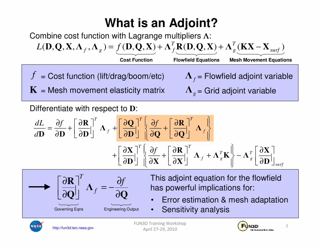
What is an Adjoint?

f

K

fΛ

gΛ

= Cost function (lift/drag/boom/etc)

= Mesh movement elasticity matrix

= Flowfield adjoint variable

= Grid adjoint variable

Combine cost function with Lagrange multipliers ΛΛΛΛ:

Differentiate with respect to D:

R Q RΛ Λ

D D D D Q Q

TT T

f f

dL f f

d

∂ ∂ ∂ ∂ ∂ = + + + ∂ ∂ ∂ ∂ ∂

T T

T T

f g g

surf

f ∂ ∂ ∂ ∂ + + + − ∂ ∂ ∂ ∂

X R XΛ Λ K Λ

D X X D

Mesh Movement EquationsFlowfield EquationsCost Function

( , , , , ) ( , , ) ( , , ) ( )T T

f g f g surfL f= + + −D Q X Λ Λ D Q X Λ R D Q X Λ KX X

T

f

f∂ ∂ = − ∂ ∂

RΛ

Q Q

This adjoint equation for the flowfield

has powerful implications for:

• Error estimation & mesh adaptation

• Sensitivity analysisGoverning Eqns Engineering Output


April 27-29, 20108

Adjoints for Error Estimation and Mesh Adaptation

It is apparent that:

ff∂

≡∂

ΛR

Direct relationship between local equation

error and the output we are interested in!

• These relationships can be used to get error estimates on

• Also used to compute a scalar field explicitly relating local point spacing requirements to output accuracy for a user-specified error tolerance

• Often yields non-intuitive insight into gridding requirements

• Relies on underlying mathematics to adapt, rather than heuristics such as solution gradients

Blue=Sufficient ResolutionRed=Under-Resolved

Transonic Wing-Body:

“Where do I need to put grid points

to get 10 drag counts of accuracy?”f

User no longer required to be a

CFD expert to get the right answer


April 27-29, 20109

Supersonic Adjoint-Based Mesh Adaptation

• Objective: Adapt grid to compute drag on

lower airfoil as accurately as possible

• Result of adjoint-based adaptation:

• Uniformly-resolved shocks are not required

• Drag is computed accurately with a

90% smaller grid

Adjoint-Based AdaptationCD=0.0766 3,810 Nodes

Feature-Based AdaptationCD=0.0767 37,352 Nodes

3M∞

=

Collaboration with Venditti/Darmofal of MIT using FUN2D


April 27-29, 201010

Adjoint-Based Mesh Adaptation for High LiftCollaboration with Venditti/Darmofal of MIT using FUN2D

• Initial grid was coarse Euler mesh

• Pressure-based indicator only resolves strong flow curvature

• Adjoint-based indicator also includes important smooth regions, stagnation streamline and wakes

http://fun3d.larc.nasa.gov 11FUN3D Training Workshop

April 27-29, 2010

Adjoints for Sensitivity AnalysisExamine the remaining terms in the linearization:

T T TT T

f f g gsurf

dL f f

d

∂ ∂ ∂ ∂ ∂ ∂ = + + + + − ∂ ∂ ∂ ∂ ∂ ∂

R X R XΛ Λ Λ K Λ

D D D D X X D

RK Λ Λ

X X

T

T

g f

f ∂ ∂ = − +

∂ ∂

Discrete adjoint equation

for mesh movement

T T

f g

surf

dL f

d

∂ ∂ ∂ = + − ∂ ∂ ∂

R XΛ Λ

D D D D

Sensitivity

equation

∴

Function Evaluation Sensitivity Evaluation

1. Compute surface mesh at current D

2. Solve mesh movement equations

3. Solve flowfield equations

3. Solve flowfield adjoint equations

2. Solve mesh adjoint equations

1. Matrix-vector product over surface

Analysis Cost = Sensitivity Analysis Cost

Even for 1000’s of design variables


Design Variables in FUN3D

• Global flowfield variables– Mach number, angle of attack

• Shape variables– These depend entirely on the geometric parameterization being

supplied to FUN3D; FUN3D has no native shape variables, other than the grid points themselves

• Additional variables related to unsteady simulations


April 27-29, 201012


Objective/Constraint Functions in FUN3D


April 27-29, 201013

*

1

( )i

j

Jp

i j j j

j

f C Cω

=

= −∑ ω = weight C = aero coeff

p = power C∗= target aero coeff

• User may specify which boundary patch in the grid (or all) to which each function applies

• Constraints may be explicit or added as “penalties”

• Multipoint/multiobjective: as many composite functions/constraints as desired

– Only limited by particular optimization package

– Adjoints for multiple functions/constraints computed simultaneously

• The optimization always seeks to minimize the objective function(s), so pose them accordingly


Geometry Parameterizations


April 27-29, 201014

• FUN3D relies on a pre-defined relationship between a set of parameters, or design variables, and the discrete surface mesh coordinates

• Given D, surface parameterization determines Xsurf (surface mesh)

• For example, given the current value of wing thickness at a location, what are the corresponding xyz-coordinates of the mesh?

• This narrows down the number of design variables from hundreds of thousands (raw grid points) to dozens or hundreds

– Optimizers will perform more efficiently

– Smoother design space

• The other requirement of the parameterization package is that itprovides the Jacobian of the relationship between the design variables and the surface mesh, ∂Xsurf/∂D

• While FUN3D users may provide their own parameterization scheme, most choose to use one of two Langley-provided packages based on free-form deformation algorithms:

– MASSOUD: Aircraft-centric design variables (thickness, camber, planform, twist, etc)

– Bandaids: General patching tool to handle fillets, winglets, and other odd shapes

– Both packages maintained by Jamshid Samareh of NASA LaRC

• To dump out the surface grids in the Tecplot format necessary for these tools, run the flow solver with ‘--write_massoud_file’

– This procedure generates a [project]_massoud_bndryN.dat file for the ith solid boundary

Wing Twist via MASSOUD


Design/description.i

• i suffix is an integer referring to the

design point (to accommodate multipoint

design)

• Contains all of the baseline files

describing this design point (CFD model

and all input decks specific to it)

• The optimization never changes anything in here; this is where the

optimizer can always find the problem

definition

• You provide the problem description for the ith design point here

Directory Tree for FUN3D-Based Design


April 27-29, 201015

Design• Main directory for design execution

• The only directory here without a hardwired name

Design/ammo

• Design is executed from here using the opt_driver

executable

• ammo.input resides here

Design/model.i• i suffix is an integer referring to

the design point (to accommodate

multipoint design)

• All CFD runs are performed here

• You never change anything in here; it only contains outputs

Design/model.i/Flow

• All flow solutions are

performed here

Design/model.i/Adjoint

• All adjoint solutions are

performed here

Design/model.i/Rubberize

• All MASSOUD evaluations are

performed here

Design/model.i/Rubberize/surface_history

• A Tecplot file for every surface grid evaluated during the design is stored here

You need not set up this tree manually; the code will do it for you,

provided some basic pathnames


Demo: Maximize L/D for Transonic Flow Over a Wing

• Log into your account on cypher-work14

• Go down into the Design_Demos directory

‘cd Design_Demos’

• Go down into the Wing directory

‘cd Wing’

• To build the directory tree we just described, you would normally run‘/path/to/your/FUN3D/installation/Design/opt_driver --setup_design 1’

– After entering a couple of pathnames, it would build the tree for you


April 27-29, 201016

ONERA M6 Wing:

Baseline L/D=6.7


• Do an ‘ls’ in your current directory

• You will see the following directory structure:

– The ammo subdirectory contains the high-level inputs for the optimization

• You will set up one file in here to control the actual optimization

– The description.1 directory must contain all of the baseline files related to the first

design point (grid, parameterization, solver input deck, etc)

• This is the primary location you need to fill up with input files ahead of time

• During the course of the optimization, the codes will always look here for the baseline files

related to the first design point

• The optimization procedure will never write to this directory; it is designed to store the

problem definition

– The model.1 directory contains three subdirectories in which the actual CFD will be

performed for the first design point:

• Adjoint is where the adjoint solutions will take place

• Flow is where the flow solutions will take place

• Rubberize is where the parameterizations are evaluated

– You do not need to set anything in the model.1 directories – they will be populated

during the course of the design and only contain outputs


April 27-29, 201017



• Go down into the description.1 directory

• These are the files you would normally have to provide in the description.i

directory for a typical design – let’s walk through and look at each of them…


April 27-29, 201018


• This file is used to specify any command line options (CLO’s) required by each

of the FUN3D executables

• The first line specifies the number of executables for which you are providing

CLO’s

• This is followed by a line containing an integer and a keyword

– The integer specifies the number of CLO’s you are providing for the code identified by the keyword

• This is followed by the actual CLO’s for the current executable

• Note ‘mpirun’ is an available keyword: this provides the opportunity to feed your mpirun executable any options it may require (-nolocal,

-machinefile filename, etc.)

– Depends on your environment, queue structure, etc.

command_line.options


• These files are input files for MASSOUD for the 1st body; the MASSOUD setup

tool provides these when you set up your parameterization

• Do not change these files


April 27-29, 201019

design.1, design.gp.1

• This file is an input file for MASSOUD for the 1st body; the MASSOUD setup tool

provides this template when you set up your parameterization

• Depending on how you choose to “link” raw MASSOUD variables to create new

variables, this defines the linking weights (see MASSOUD documentation)

• When using MASSOUD with FUN3D, you must always use the design variable

linking option, even if simply set to the identity matrix

design.usd.1



• This file tells MASSOUD the names of its input/output files for the 1st body

• The first value specifies the number of linked MASSOUD design variables

– If linking matrix is identity, this is just the number of raw MASSOUD design variables

• The remainder of the inputs are filenames; they should remain as is, but with

the integer value in each name set to the index of the current body


April 27-29, 201020

massoud.1



• This is the nominal solver input deck for your case

• The adjoint solver also uses this input

– If the adjoint requires different values (e.g., stopping tolerance), you can override these values with CLO’s given in command_line.options

• It should contain the necessary inputs to run the baseline case

• The optimization will override values as needed using CLO’s (e.g., angle of

attack, etc)


April 27-29, 201021

fun3d.nml

• This is the nominal mesh for your baseline case

• This particular grid is in FAST format; VGRID format is also allowed

• Note the symmetry plane has been given a 3080 BC index – this is

recommended for symmetry planes during design optimization

inviscid.fgrid, inviscid.mapbc



April 27-29, 201022

• This file is used to define the design variables and their bounds, objective

functions, and constraints for the current design point

• A copy of this file is placed in the model.1 directory at the beginning of an

optimization and is continuously updated with the current values of the design

variables, objective/constraint functions, and all gradient information

– If you want to know the latest info during a design, it’s probably in here

rubber.data



April 27-29, 201023

Code Status Block

• Leave alone

Design Variable Block

• In general, for each design variable, you must set several fields

– Active (0=no, 1=yes), baseline value, upper and lower bounds (if active)

• First subsection lays out the Mach number and angle-of-attack information

• This is followed by an input stating the number of bodies to be designed

• Then for each body:

– Fixed number of rigid motion variables – leave these alone

– Number of shape variables and their inputs – these correspond directly to the MASSOUD variables previously discussed

• When setting bounds for shape variables, it pays to be conservative – the optimizer will exploit every radical shape it can dream up

• You can quickly get into unsolve-able or invalid/crossed-up geometries

• You can always loosen up the bounds and restart the design if needed


rubber.data


April 27-29, 201024

Function Block

• These sections lay out the objective/constraint function definitions

• First input is the total number of composite functions being specified (sum of

objectives + constraints)

• Then, for each function:

– Is it an objective function (1) or a constraint (2)

– If it is a constraint, what are the upper and lower bounds (otherwise dummies)

– How many component functions are used to build up the composite function

– Time step interval defining the function (leave as dummies – for unsteady design)

– Then the list of component functions:

• Boundary index it applies to (0 means all boundaries)

• Keyword identifying the function type

(see header of LibF90/forces.f90)

• Value (dummy – this is an output during the optimization)

• Weight to be applied to current component function

• Target value for current component function

• Exponent for current component function

• The remainder of the function block is devoted to sensitivity outputs – you can place dummies here, but there must be a line corresponding to every design variable


Our objective function:2

( / 20)f L D= −

rubber.data


April 27-29, 201025

• We are now finished setting things up in the description.1 directory

• Finally, head over to the ../ammo directory

• There is only a single file here that needs to be set up

– The ammo.input file controls the actual optimization procedure

• Let’s walk through this file real quick...


• Change USERNAME to your username in the absolute path variable

• Everything else documented on the website, but a few reminders:

– Optimization packages: KSOPT=3, PORT=4, NPSOL=5

– Grid types: FAST=1, VGRID=2

– Operation to perform: analysis=1, sensitivity analysis=2, optimization=3

– Note you can specify the mpirun executable name

• Useful if executable is called ‘mpiexec’ or otherwise on your system

ammo.input


April 27-29, 201026

Enough with problem setup, let’s do something already!

• The first thing I typically do is just run a function evaluation to see that the

parameterization and all of the inputs are set correctly

• To do this, edit ammo.input and set Operation to Perform to 1

• The command line that is used to run this case is

opt_driver --sleep_delay 5 > screen.output

– The ‘--sleep_delay 5’ instructs the driver to wait 5 seconds in between operations – allows

NFS caching to keep up

• Submit the job using ‘qsub qinput’



April 27-29, 201027

• The first thing that you will see is MASSOUD evaluating the parameterization for each body, defining the surface grid coordinates at the baseline position

• The flow solver will then start up, but prior to the solve, you will see an auxiliary solution take place that represents the interior mesh movement based on the elasticity equations

– For this first step at the baseline position, you should see very small numbers for the “Error

Estimate”: this indicates the current mesh is very close to the desired mesh

• After the actual flow solution takes place, the solver will evaluate each of the objective

and constraint functions you posed:Current value of function 1 176.932026370194

• This marks the end of a successful function evaluation

• Always wise to plot the flow solver convergence – you want to run enough iterations to get a “reasonable” answer, but you don’t necessarily need to drive it into the ground



April 27-29, 201028

• Now lets try a sensitivity analysis

• Edit ammo.input and set Operation to Perform to 2

• Submit the job

• The first thing that will take place is a function evaluation, just as before

• After the function evaluation takes place, MASSOUD will fire up again to

evaluate the linearizations of the surface mesh coordinates with respect to the

design variables

• FUN3D’s adjoint solver will then start up:

– You will see a solution taking place; this is the flowfield adjoint

– Afterwards, you will see another solution occurring; this is the elasticity adjoint for the mesh

– The final step is to update the model.1/rubber.data file with the sensitivity

information

• This marks the end of a successful sensitivity analysis

• Again, it is wise to plot the convergence of the flowfield adjoint system

– This convergence history is in the model.1/Adjoint/inviscid_hist.tec file

– In general, you want 2-3 orders of magnitude convergence; this is usually sufficient for reasonable sensitivity information



April 27-29, 201029

• If you got this far, things are looking pretty good – we’ve checked that

everything is set up to run functions and gradients correctly, which is all the

optimizer depends on

• Now we’re ready to try an actual optimization

– Edit ammo.input and set Operation to Perform to 3; submit the job

• Now you will see a lot of function and gradient evaluations going by, as the

optimizer starts to change design variables and search for an optimum solution

• One easy way to monitor progress is to:– ‘grep “Current value” screen.output’:

Current value of function 1 176.932026370194











• You can also observe (but don’t change!) the file model.1/rubber.data



April 27-29, 201030

• After the job finishes, PORT will summarize its performance in the file model.1/port.output

• Since each solution is a warm start, you can plot the entire flow solution history contained in model.1/Flow/inviscid_hist.tec

• A history of the surface geometry is stored in model.1/Flow/movie.tec

– Use Tecplot’s animate capability to view the evolution of the

geometry/solution


Redesigned Wing:

L/D=10.1


April 27-29, 201031

What Could Possibly Go Wrong?

• The procedure can terminate due to CFD-related problems:

– Running into negative volumes during a mesh movement (you can plot the

history of the surface(s) using the files in model.1/Rubberize/surface_history)

• Watch for invalid surfaces or unusually large changes

• Be conservative in your lower/upper bounds!

– The flowfield or the adjoint solution is unstable

• Problem-dependent; get in touch for advice

• The procedure can also terminate due to hardware/environment

problems

– You run out of allocated time, a node dies, etc.

• Finally, the procedure can terminate if the optimizer has given up:

– No more progress can be made due to constraints

– The optimizer has hit the max number of functions/gradients you allowed

– An optimal solution has been found



List of Key Input/Output Files

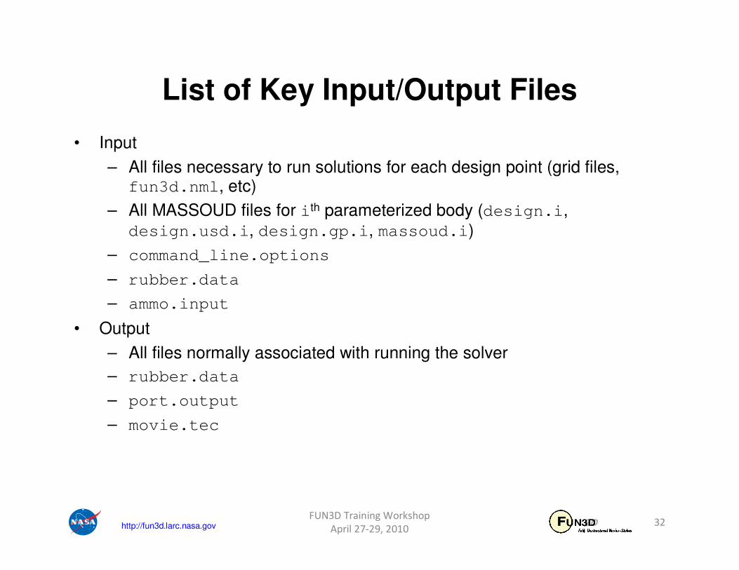
• Input

– All files necessary to run solutions for each design point (grid files, fun3d.nml, etc)

– All MASSOUD files for ith parameterized body (design.i,

design.usd.i, design.gp.i, massoud.i)

– command_line.options

– rubber.data

– ammo.input

• Output

– All files normally associated with running the solver

– rubber.data

– port.output

– movie.tec


April 27-29, 201032


April 27-29, 201033

• That’s more or less the basic pieces involved with running an optimization

• Lots of options we did not cover here; see website or get in touch for help

– How the wrappers work (LibF90/analysis.f90, LibF90/sensitivity.f90)

– Parameterizations other than MASSOUD

– Multipoint/multiobjective (tutorial on website)

– Constrained problems (tutorial on website)

– Running with other optimization packages (tutorial on website)

– Body grouping, spatial transforms

– Forward-mode sensitivity analysis using complex variables

– Unsteady design (expensive)

General Advice

• Become very comfortable with the flow solver

• Work the website tutorials

• Learn how to set up parameterizations using MASSOUD and/or bandaids

• Try plugging in your own grids/parameterizations in the tutorials

• Ask questions – it’s actually not that bad once you get up the learning curve

Summary of FUN3D-Based Design Optimization


What We Learned• General approach used by FUN3D for design optimization

• What is an adjoint

• What does a function/gradient evaluation consist of in terms of CFD

• Design variables in FUN3D

• Functions/constraints in FUN3D

• What is required of a geometry parameterization tool

• How to set up the inputs required for design optimization

• How to run function, gradient evaluations

• How to perform a basic design optimization

• What to watch out for and how to interpret results


April 27-29, 201034

Have fun and don’t hesitate to send questions our way!

[email protected]

Documents

Session 14: Adjoint-Based Design Optimization · PDF fileSession 14: Adjoint-Based Design Optimization ... – You must download and install your choice of these third-party libraries