Defence nationals AD-A263 661 UNCLASSIFIEDSl~~lilllillli~ l i~lllllN ll

t~~ ~~~~ I 1 1111 ILI I ILLI1 1 I!HI 115 31ýSUFFIELD REPORTl

RII# NO. 582

UNLIMITEDDISTRIBUTION

EXPERIMENTAL STUDY OF LOCATION AND

IDENTIFICATION OF FERROUS SPHEROIDS USING

A "SMART" TOTAL FIELD MAGNETOMETER

DTICSELECTEMAY 'A5 193,l

DITXTTCýSTETAbyc 11CAppr )ed ti pubimo t04.G

Di .uu= a=•....d

John E. McFee, Robert Ellingson and Yogadhish Das

% A o -93-09604January' 1993 lilI Il jjI I I 1111 i lI

k DEFENCE RESEARCH ESTABLISHMENT SUFFIELD: RALSTON: ALBERTA

I WARNING

"The use of this information is permitted subject torecognition of propriutnrv y -1 patent rights'.Canada

UNCLASSIFIED

DEFENCE RESEARCH ESTABLISHMENT SUFFIELDRALSTON, ALBERTA

SUFFIELD REPORT NO. 582

EXPERIMENTAL STUDY OF LOCATION AND

IDENTIFICATION OF FIERROUS SPHEROIDS

USING A "SMART" TOTAL FIELD MAGNETOMETER

by

John E. McFee, Robert Ellingson and Yogadhish Das

DTIC QUALMIY INSPECTED 5

Acceslori ForNTIS CRA&MDTiC TA8 UUnannounced UJustification

By .___

Distribution II WARNING •

I The use of this information is permitted subject to Avadability Codesrecognition of proprietary and patent right . ,, _

Avail andlor01sl Special

UNCLASSIFEDE-1 ,

UNCLASSIFIED

iiUNC~LA~SSIEDE DRES-SR-582

UNCLASSIFIED

ABST4~

A microprocessor-controlled magnetometer which accurately locates and identifiescompact ferrous objects in real-time is described. The person-portable instrument consistsof a cart-mounted cesium magnetometer, optical encoder, microcontroller, interface andlaptop computer. The instrument guides the operator to collect simultaneous magnetic fieldand position data in a horizontal plane above an object. Custom algorithms estimatelocation and dipole moment and use the latter to classify the object. Data collection takes6 - 13 minutes, location and moment estimation 5 seconds, classification 30 seconds.Experiments using two ferrous spheroids and studies using magnetic total field and verticalcomponent magnetic maps generated by a mathematical computer model are described.Limits of error in estimation of location and dipole moment, error in classification, andrelative effects of sources of error are quantified. The rms error for location vectorcomponents was 0.019 m - 0.045 m compared to the average precision of 0.003 m - 0.005 m.The average magnitude of the difference between estimated and theoretical dipole momentvectors as a percentage of the theoretical dipole moment was 24.5±11.4% compared toprecision uf 0.51 - 8.21%. Pattern classification with a computer generated dipole momentdesign set is , escribed. Deviation between experimental moment estimates and thecomputer model degraded performance but the misclassification rate for the two objects forwhich experimental measurements were made was 11.1%. If an experimental design setwere used, analysis shows that tht limiting misclassification error for the presentexperimental precision should be between 2 and 5%.

iii

DRES-SR-e•2 .UNCLASSIFIED

*1 ~NON CLASSIFI

On decrit un magndtom~tre, pilot6 par un micropi ocesseur, qul permet de localiseret d'identifier rapidement en temps rdel des objets ferreux compacts. L'appareil, qui peut8tre porte par itne personne, est constitu6 d'un magntetvm~re au cesium, d'un codeuroptique, d'un micro**contr6leur, d'une interface et d'un ord'nateur portatif, le tout monte surun chariot. L'appareil permet A l'utilisateur d'obtenir simultanement des donndes sur lechamp magndtique et la position dans un plan horizontal au-dessus d'un objet. Desalgorithmes 6labores sur mesure permettent d'estimer le moment dipolaite et sa positionet d'utiliser ces donn6es pour classer l'objet. 11 faut de 6 A 13 minutes pour obtenir lesdonndes, 5 secondes pour estimer le moment et ia position et 30 secondes pour classer1'objet. On decrit des experiences avec deux sph6roides ferreux, ainsi que des 6tudeseffectudes avec des cartes du champ magnetique total et de la composante magnetiqueverticale, produites ýt l'aide d'un mod~le mathematique sur ordinateur. On determine1'importance des limites d'erreur sur 1'estimation du moment dipolaire et de sa position, deFerreur de classement, ainsi que des effets relatifs des sources d'erreur. L'erreur1 quadratique moyenne sur les composantes du vecteur de position etait de 0,019 m -

I ~0,045 m, en coinparaison avec la precision moyenne de 0,003 m - 0,005 ni. La grandeurmoyenne de l'ecart entre la valeur estimde et la valeur thdorique des vecteurs du momentdipolaire, exprimee en pourcentage du moment dipolaire th6orique, 6tait de 24,5 t 11,4 %

I en comparaison avec la precision qui 6tait de 0,51 - 8,21 %. On decrit le classement desresultats realises A 1'aide d'un ensemble de reference de moments dipolaires cr66 par

I ~ordinateur. L'6cart entre les moments estimes experimentalement et les valeurs obtenuespar moddlisation informatique diminuait le rendement de l'appareil; neanmoins, le taux declassement incorrect pour les deu~x spheroifdes ayant fait I'objet des mesures expdrimentalesetait de 11,1 %. L'analyse rev~le que, pour un ensemble de reference experimrental, lalimite d'erreur de classement devrait 8tre comprise entre 2 et 5 % pour la pr~senteprecision expdrimentale.

DRES-SR-582 NON CLASSIFIt

UNCLASSIFIED

RESUME

ii

UEi

ivUNCILASSIFIED DRES-SR-582

S. .. . . . .. . . . . . .. . . . .. . . . . L , . . . . . . . . .. .._. . . .._ I" . . . .. . .. .. . .. . . . .. . ... . . . . . . . . . .. . .

UNCLASSIFIED

Executive Summary

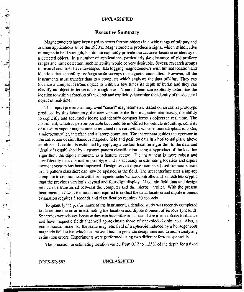
Magnetometers have been used to detect ferrous objects in a wide range of military andcivilian applications since the 1930's. Magnetometers produce a signal which is indicativeof magnetic field strength, but do not explicitly provide the accurate location or identity of"a detected object. In a number of applications, particularly the clearance of old artilleryranges and mine detection, such an ability would be very desirable. Several research groupsin several countries have developed data logging magnetometers with limited location andidentification capability for large scale surveys of magnetic anomalies. However, all theinstruments must transfer data to a computer which analyses the data off-line. They can

A .• localize a compact ferrous object to within a few times its depth of burial and they canclassify an object in terms of its rough size. None of them can explicitly determine thelocation to within a fraction of the depth and explicitly determine the identity of the detectedobject in real-time.

This report presents an improved "smart" magnetometer. Based on an earlier prototypeproduced by this laboratory, the new version is the first magnetometer having the abilityto explicitly and accurately locate and identify compact ferrous objects in real-time. The

-: instrument, which is person-portable but could be modified for vehicle mounting, consistsof a cesium vapour magnetometer mounted on a cart with a wheel-mounted optical encoder,a microcontroller, interface and a laptop computer. The instrument guides the operator in

4,• I the collection of simultaneous magnetic field and position data in a horizontal plane abovean object. Location is estimated by applying a custom location algorithm to the data andidentity is established by a custom pattern classification using a byproduct of the locationalgorithm, the dipole moment, as a feature vector. The instrument is more robust anduser friendly than the earlier prototype and its accuracy in estimating location and dipolemoment vectors has been improved. Design sets of dipole moments (used for compalisonin the pattern classifier) can now be updated in the field. The user interface uses a lap-topcomputer to communicate with the magnetometer's microcontroller and is much less cryptic

J than the previous version's keypad and four digit display. Magi :tic field data and designsets can be transferred between the computer and the microc -troller. With the presentinstrument, as few as 6 minutes are required to collect the data, location and dipole moment

estimation cequires 5 seconds and classification requires 30 seconds.

To quantify the peformance of the instrument, a detailed study was recently completedto determine the error in estimating the location and dipole moment of ferrous spheroids.Spheroids were chosen because they can be similar in shape and size to unexploded ordnanceand have magnetic fields that well approximate those of unexploded ordnance. Also, amathematical model for the static magnetic field of a spheroid induced by a homogeneousmagnetic field exists which can be used both to generate design sets and to aid in analysingestimation errors. Experiments were performed using two different ferrous spheroids.

The precision in estimating location varied from 0.12 to 1.35% of the depth for a fixed

vDRES-SR-582 UNCLASSIFIED

UNCLASSIFIED

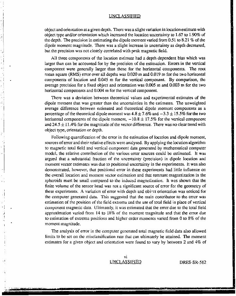
object and orientation at a given depth. There was a slight variation in location estimate withobject type and/or orientation which increased the location uncertainty to 1.67 to 1.90% ofthe depth. The precision in estimating the dipole moment varied from 0.51 to 8.21 % of thedipole moment magnitude. There was a slight increase in uncertainty as depth decreased,but the precision was not closely correlated with peak magnetic field.

All three components of the location estimate had a depth dependent bias which waslarger than can be accounted for by the precision of the estimation. Errors in the verticalcomponent were generally larger than those for the horizontal components. The rootmean square (RMS) error over all depths was 0.020 m and 0.019 m for the two horizontalcomponents of location and 0.045 m for the vertical component. By comparison, theaverage precision for a fixed object and orientation was 0.005 m and 0.003 m for the twohorizontal components and 0.004 m for the vertical component.

There was a deviation between theoretical values and experimental estimates of thedipole moment that was greater than the uncertainties in the estimates. The unweightedaverage difference between estimated and theoretical dipole moment components as apercentage of the theoretical dipole moment was 4.8 ± 7.6% and -3.3 ± 15.5% for the twohorizontal components of the dipole moment, - 10.8 ± 17.5% for the vertical componentand 24.5 ± 11.4% for the magnitude of the vector difference. There was no clear trend withobject type, orientation or depth.

Following quantification of the error in the estimation of location and dipole moment,sources of error and their relative effects were analysed. By applying the location algorithmto magnetic total field and vertical component data generated by mathematical computermodel, the relative contribution of the various error sources could be estimated. It wasargued that a substantial fraction of the uncertainty (precision) in dipole location andmoment vector estimates was due to positional uncertainty in the experiments. It was alsodemonstrated, however, that positional error in these experiments had little influence onthe overall location and moment vector estimation and that remnant magnetization in thespheroids must be small compared to the induced magnetization. It was shown that thefinite volume of the sensor head was not a significant source of error for the geometry ofthese experiments. A variation of error with depth and obi,-ct orientation was noticed forthe computer generated data. This suggested that the main contributor to the error wasestimation of the position of the field extrema and the use of total field in place of verticalcomponent magnetic data. Ultimately, it was estimated that the error due to the total fieldapproximation varied from 14 to 18% of the moment magnitude and that the error dueto estimation of extrema positions and higher order moments varied from 0 to 8% of themoment magnitude.

The analysis of error in the computer generated total magnetic field data also allowedlimits to be set on the misclassification rate that can ultimately be attained. The momentestimates for a given object and orientation were found to vary by between 2 and 4% of

viUNCLASSIFIED DRES-SR-582

UNCLASSIFIED

the moment magnitude as the depth varied. If the estimated moments were used in thedesign set, this suggests that the limiting misclassification error would be between roughly1.4 and 2.4% if the experimental (mainly positional) error were substantially less than thealgorithmic and approximation errors. For the present experimental precision (4.1 ± 3.0%), the misclassification error should be roughly between 2 and 5% (assuming quadratureerror summation) if the design set were experimentally obtained.

Pattern classification was performed with a computer generate dipole moment design setconsisting of 8 objects including the 2 used in these experiments. The gross misclassificationrate was 10.3% for the class number 4 spheroid and 100% for class number 6. Closerexamination revealed that class 6 was always classified as class number 3, which is asimilarly shaped spheroid. This is likely due to the deviation between the moment estimatesfor the experimental spheroid and the computer model. The repeatability of classification,

that is, the percentage of cases in which an object is classified as the same class, is a bettermeasure of classifier performance. The repeatability of classification was 91.7%. If weconsider only the two objects for which experimental measurements were made, we seethat only 4/36 cases (11.1%) were classified incorrectly.

The overall performance of the smart magnetometer is very encouraging. The reportcloses with a discussion of future work that must be done to improve the instrument and tomake it successful as a practical locator and identifier for buried ferrous ordnance.

"viiDRES-SR-582 UNCLASSIFIED

I .UNCLASSIFIED

U

viiiUNCLASSIFIED DRES-SR-582

UNCLASSIFIED

i

ACKNOWLEDGEMENT I

The authors would like to thank Mr. Ian Lawson who, while a Summer ResearchAssistant in the Threat Detection Group, assisted in the collection and processing of thedata presentexl in this report.

This work was supported under Chief Rearch and Development Project Number031SD.

I

mi•a

ixDRES-SR-582 I.J•CLASSIFIED

UNCLASSIFIED DRES-SR-582

UNCLASSIIED

Table of Contents

Abstract iii

RWsum6 iv

Executive Summary v

Acknowledgement viii

Table of Contents xi

List of Figures xiii

List of Tables xvi

1 Introduction 1

2 Theory 5

2.1 Magnetic Field Measurement ............................. 5

2.2 Estimation of Dipole Location and Moment ..................... 6

2.3 Id11 t1t~1fUnAf%~ a3 V"Ier0 'dFrom 1- Dipo~le~ ...............

2.4 Multipole Expansion of the Magnetic Field of a Spheroid ............ 10

3 Experimental Method 15

3.1 The Smart Magnetometer ....... ....................... 15

3.2 Experimental Layout ................................... 20

3.3 Procedure .......... ................................ 22

xiDRES-SR-582 UNCLASSIFIED

UNCLASSIFIED

3.4 Initial Calibration ....... .. ......... ..... .. .... 22

4 Experimental Results 27

5 Performance of Location Estimation 59

5.1 Sources of Error in Location Estimation ........................ 59

5.2 Location Estimates for Theoretical Total Field Data ................ 62

5.3 Location Estimates for Theoretical Vertical Component Field Data . . . . 70

6 Performance of Pattern Classification 77

7 Conclusions 85

8 References 89

XiiUNCLASSIFIED DRES-SR-582

UNCLASSIFIE[D

List of Figures

, 2.1 Geometry for magnetostatic dipole location .................... 6

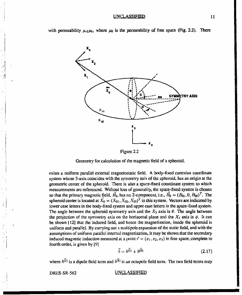
2.2 Geometry for calculation of the magnetic field of a spheroid........ .11

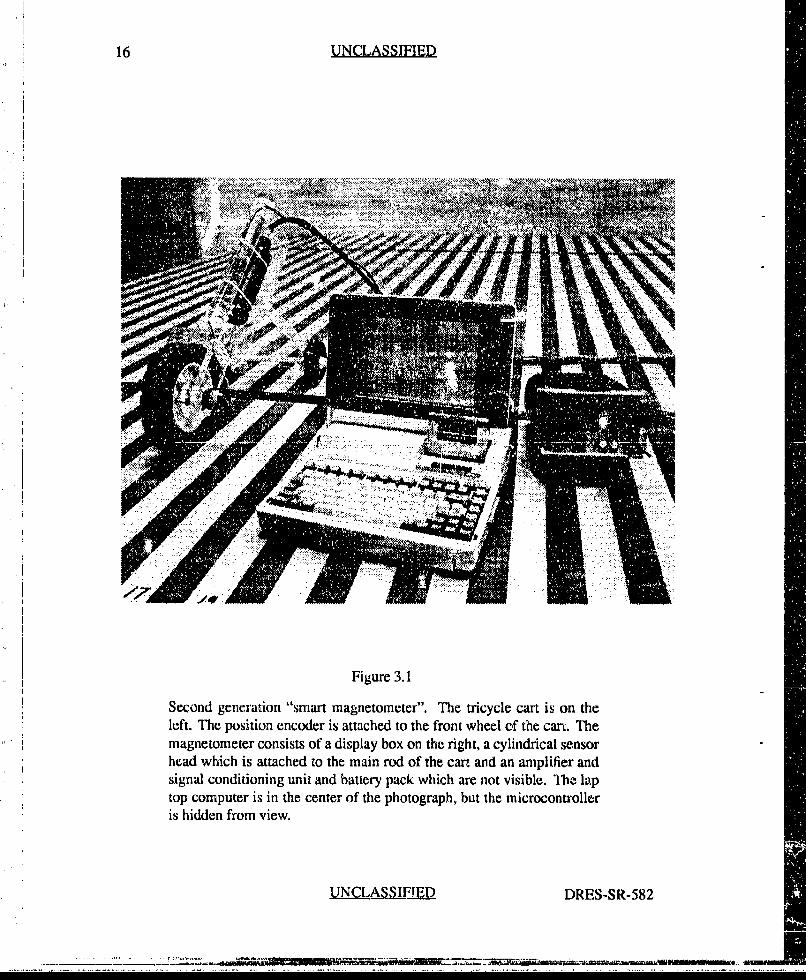
3.1 Second generation "smart magnetometer"...................... 16

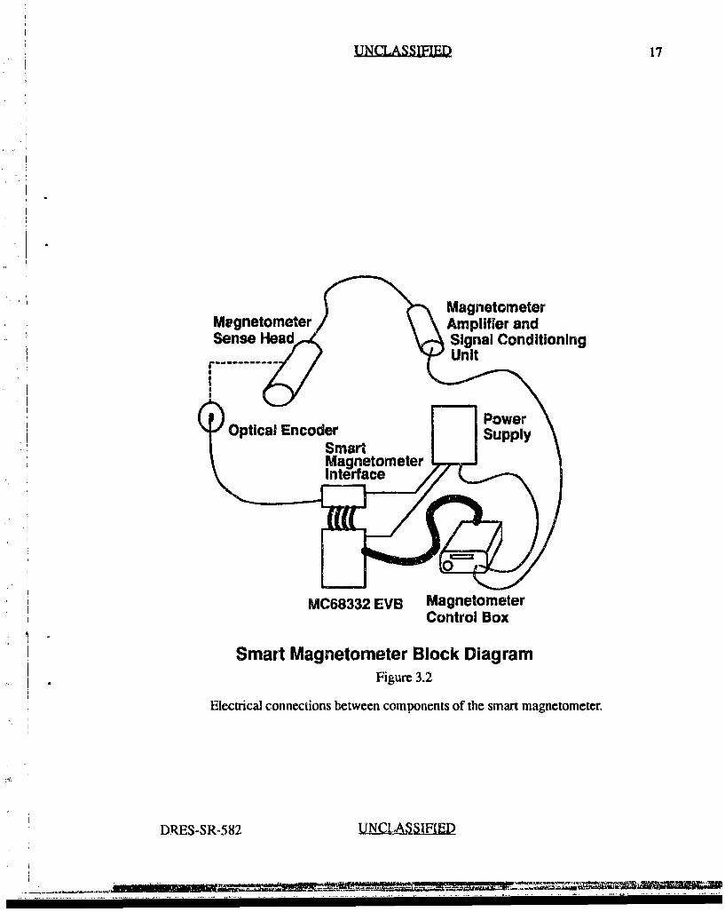
3.2 Electrical connections between components of the smart magnetometer. 17

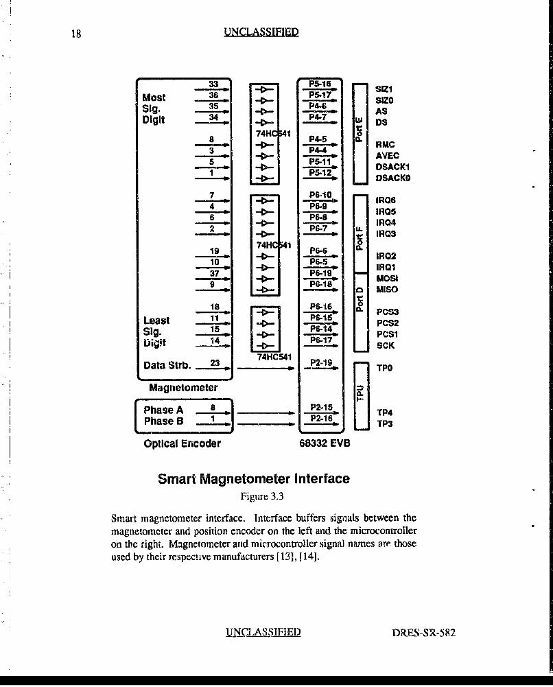
3.3 Smart magnetometer interface ............................ 18

3.4 Top view of the experimental set-up for measurement of magnetic fields ofcompact objects .................................... 21

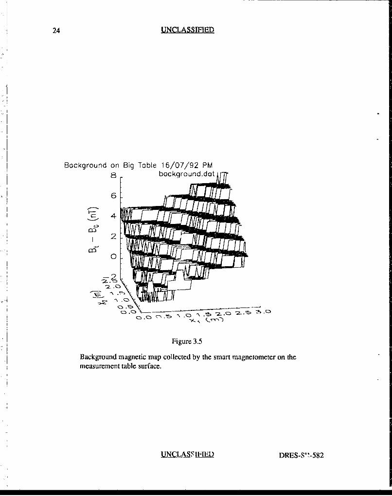
3.5 Background magnetic map collected by the smart magnetometer on themeasurement table surface .............................. 24

4.1 Measured total magnetostatic field map versus position in a horizontalplane for spheroid F at 0 = 00. Depth is 0.598 m. Ambient (earth's) fieldmagnitude has been subtracted ............................. 28

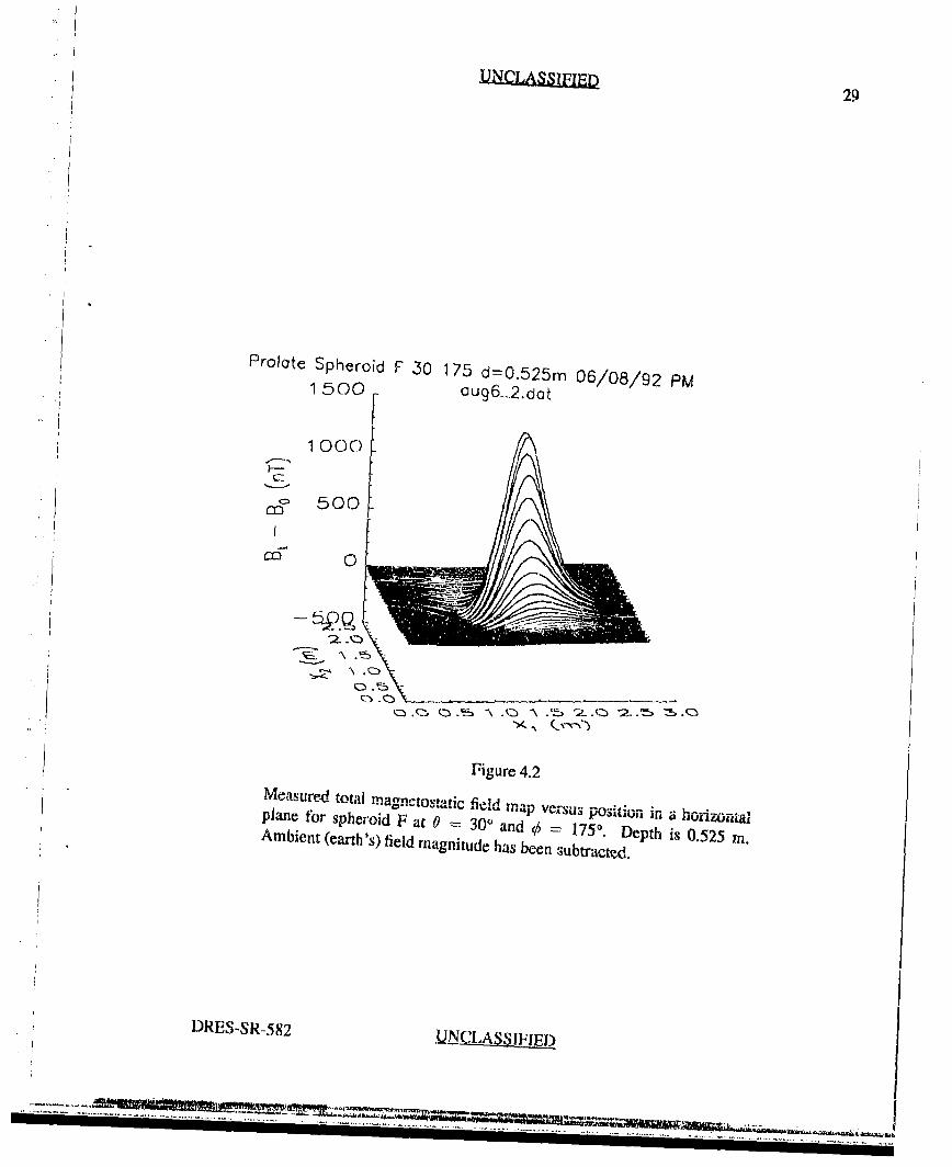
4.2 Measured total magnetostatic field map versus position in a horizontalplane for spheroid F at 0 = 30° and 0 = 1750. Depth is 0.525 m. Ambient(earth's) field magnitude has been subtracted ................... 29

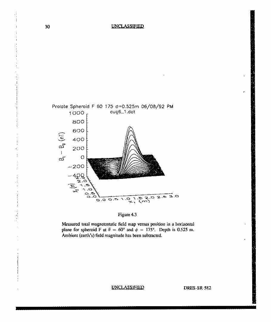
4.3 Measured total magnetostatic field map versus position in a horizontalplane for spheroid F at 0 = 60' and 4. 1750. Depth is 0.525 m. Ambient(earth's) field magnitude has been subtracted ................... 30

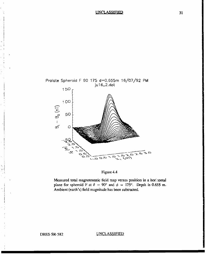
4.4 Measured total magnetostatic field map versus position in a horizontalplane for spheroid F at 0 = 90' and ,S = 175'. Depth is 0.655 in. Ambient(earth's) field magnitude has been subtracted .................... 31

4.5 Precision in location vector estimation for the location algorithm usingexperimental data ..................................... 37

4.6 Precision in dipole moment vector estimation for the location algorithmusing experimental data .................................. 38

xiiiDRES-SR-582 UNCLASSIFIED

A ..

UNCLASSIFIED

4.7 Spheroid depth estimates as a function of depth for experimental data. Allobjects and orientations are grouped together for a given depth ....... . 39

4.8 Error in estimates of X01 component as a function of spheroid depth forexperimental data ..................................... 41

4.9 Error in estimates of X02 component as a function of spheroid depth forexperimental data ..................................... 42

4.10 Error in estimates of X03 component as a function of spheroid depth forexperimental data ..................................... 43

4.11 Estimates of M1 component of the dipole moment as a function of spheroid

depth for spheroid F at orientation 0 0 ........................ 45

4.12 Estimates of M2 component of the dipole moment as a function of spheroiddepth for object F at orientation 0 0 .......................... 46

4.13 Estimates of AM3 component of the dipole moment as a function of spheroiddepth for object F at orientation 0 0 .......................... 47

4.14 Estimates of M, component of the dipole moment as a function of spheroiddepth for object F at orientation 90 175 ........................ 48

4.15 Estimates of M2 component of the dipole moment as a function of spheroiddepth for object F at orientation 90 175 ........................ 49

4.16 Estimates of A13 component of the dipole moment as a function of spheroiddepth for object F at orientation 90 175 ........................ 50

4.17 Estimates of M, component of the dipole moment as a function of spheroiddepth for object M at orientation 90 265 ....................... 51

4.18 Estimates of M12 component of the dipole moment as a function of spheroiddepth for object M at orientation 90 265 ........................ 52

4.19 Estimates of M3 component of the dipole moment as a function of spheroiddepth for object M at orientation 90 265 ........................ 53

4.20 Difference between M, component estimate and theoretical MI, as a per-centage of the magnitude of theoretical M for two different objects and anumber of different orientations ..... .................. 54

4.21 Difference between M2 component estimate and theoretical M2 , as a per-centage of the magnitude of theoretical M for two different objects and anumber of different orientations ............................ 55

4.22 Difference between M3 component estimate and theoretical M3, as a per-centage of the magnitude of theoretical M for two different objects and anumber of diffe-rent orientations ............................. 56

xivUNCLASSIFIED DRES-SR-582

UNCLASSIFIED

4.23 Magnitude of the vector difference between estimated All and theoreticalM, as a percentage of the magnitude of theoretical MI for two differentobjects and a number of different orientations .................... 57

5.1 Theoretical total magnetostatic field map versus position in a horizontalplane for spheroid F at 0 = 00 ........ ........................ 63

5.2 Theoretical total magnetostatic field map versus position in a horizontalplane for spheroid F at 0 = 30' and =-- 1750 .................... .... 64

5.3 Theoretical total magnetostatic field map versus position in a horizontalplane for spheroid F at 0 = 60' and 0 = 1750 .................... .... 65

5.4 Theoretical total magnetostatic field map versus position in a horizontalplane for spheroid F at 0 = 90' and q =: 175 ..................... 66

5.5 rms location vector estimation error for computer generated magnetic totalfield maps for two spheroids at various orientations and a sphere ...... . 68

5.6 rns moment vector estimation error for computer generated magnetic totalfield maps for two spheroids at various orientations and a sphere ...... . 69

5.7 rms location vector estimation error for computer generated magnetic ver-tical component field maps for two spheroids at various orientations and asphere ........................................... 71

5,8 rms moment vector estimation error for computer generated magnetic ver-tical component field maps for two spheroids at various orientations and asphere ............................................ 72

xvDRES-SR-582 UINCLASSIFIED

1"R,

UNCLASSIFIED

List of Tables

SI Comparison of location and identification estimation results with and with-

out background correction ................................ 25

II Comparison of location and identification estimation results with aid with-out background correction ................................ 25

III Comparison of location and identification estimation results for magneticmaps collected with an X2 spacing between scans of 5 cm and 10 cm. . . 26

IV Two objects used for experiments. Spheroid dimensions are defined inFigure 2.2 ........ ................................. 28

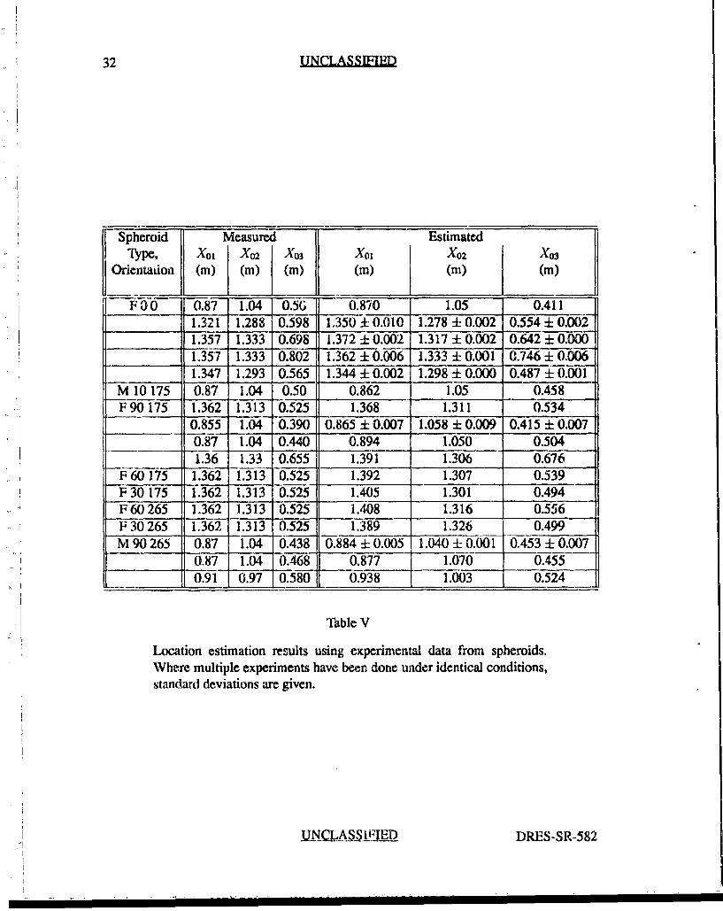
V Location estimation results using experimental data from spheroids. . . . 32

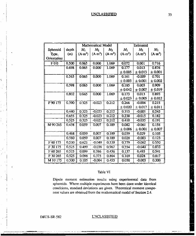
VI Dipole moment estimation results using experimental data from spheroids. 33

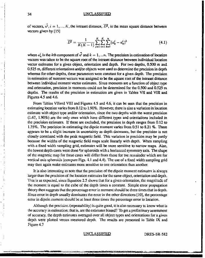
VII Precision in location vector estimation for the location estimation algorithmusing experimental data .................................. 35

VIII Precision in dipole moment vector estimation for the location algorithmusing experimental data .................................. 36

IX Spheroid depth estimates as a function of depth for experimental data. Allobjects and orientations are grouped together for a given depth ....... . 36

X Comparison of uncertainty in X3 measurement with precision of estimatedlocation and dipole moment vector components ................... 74

XI Location vector estimation results using magnetic field data generated fromthe computer model of Section 2.4 .......................... 75

XII Dipole moment vector estimation results using magnetic field data generatedfrom the computer model of Section 2.4 ........................ 76

XIII Objects used in design set for classification studies ................ 80

xviUNCLASSIFIED DRES-SR-582

UNCLASSIFIED

XIV Results of classifying dipole moments of spheroid F estimated from exper-imental magnetic field maps using the CP classifer and the design set ofTable XIII. ......................................... 81

XV Results of classifying dipole moments of spheroid M estimated from ex-perimental magnetic field maps using :he CP classifer and the design set ofTable XIII ......................................... 82

XVI Individual cases of misclassification .......................... 83

J

XviiDRES-SR-582 U~NCLAS.SIFIED

_4

IL

UNCLA~SIFIE

xviiiUNCLASSIFIED DRES-SR-582

r i.

•.

UNCLASSIFIE1 1

1. Introduction

Magnetometers have been used to detmct ferrous objects in a wide range of applicationssince the 1930's. Magnetometers produce a signal which is indicative of magnetic fieldstrength, but do not explicitly provide the accurate location or identity of a detected object.In a number of applications, particularly the clearance of old artillery ranges and minedetection, such an ability would be very desirable. Several research groups have addressedthe problem of large scale surveys to detect magnetic anomalies. A vehicle-towed detectorarray, STOLS, has been developed by Geo-Centers Inc., Newton Falls, MA, USA, for theUS Navy [1] to locate magnetic anomalies over areas of several thousand square meters.The device consists of a set of commercially available cesium vapour magnetometers anda microwave triangulation position measurement systerm connected to a data collectionsystem. Data is processed off-line to produce field intensity maps which can be interpretedto roughly locate magnetic objects. Further, compact magnetic objects such as artilleryshells can be located more accurately and roughly grouped in size, based on dipole strength,using a fairly slow iterative nonlinear least squares fit dipole locator algorithm originallydeveloped by our laboratory [2]. Another large area magnetic field mapping instrument, theTM-3, has been developed by the University of New England, Australia [3]. This hand-heldinstrument, which is based on a single cesium vapour sensor, uses a data logger to collect amagnetic field map. Data is transferred to a PC which produces images of the magnetic fieldin a plane and allows rough localization and identification of anomalies by visual inspectionof the shape of the magnetic field. Institut Dr. Forster, Reutlingen, Germany, manufactures ahand-held fluxgate gradiometer, the FEREX CAST 4.021.06, which is intended for smallerareas. It can log data while scanning an area, then transfer the data to a PC for off-lineanalysis 141. A similar data logging magnetometer with a PC analysis package, calledCAMAD, was announced some time ago by Aprotec Ltd., Manchester, UK [5], but nothinghas been heard of it since the initial announcement. All these instruments must transferdata to a computer which analyses the data off-line. They can localize a compact ferrousobject to within a few times its depth of burial (the exception being STOLS using the DRESiterative location algorithm) and can classify an object in terms of its rough size. None ofthem can explicitly determine the location to within a fraction of the depth and explicitlydetermine the identity of the detected object in real-time.

In [6], a real-time method to explicitly estimate the location and determine the identityof a compact ferrous object was presented. It was based on sampling the magnetic field

DkES-SR-582 LdNCA SIFIED

2 UNCLASSIFIED

of the object in a horizontal plane, storing simultaneous position and magnetic field data,and then using a noniterative algorithm to determine the lecation and components of thedipole moment associated with the object. A byproduct of the location algorithm was anestimate of the dipole moment which was used by a DRES continuous parameter (CP)pattern classifier to identify the object. A prototype microprocessor-controlled cesiumvapour "smart" magnetometer was described which collected simultaneous magnetic andposition data and then used these algorithms to locate and identify ferrous spheres andspheroids. A few preliminary results were also reported. This was the first magnetometerwith the ability to explicitly locate and identify compact ferrous objects and the first totalfield magnetometer witii explicit object location estimation in a self-contained instrument.

This report presents an improved "smart" magnetometer. The new version is the firstmagnetometer having the ability to explicitly and accurately locate and identify compactferrous objects in real-time. The instrument, which is person-portable, consists of a ce-sium vapour magnetometer mounted on a cart with a wheel-mounted optical encoder, amicrocontroller, interface and a laptop computer. The instrument guides the operator inthe collection of simultaneous magnetic field and position data in a horizontal plane abovean object. Location is estimated as before by applying the DRES noniterative locationalgorithm to the data and identity is established by pattern classification using the dipolemoment as a feature vector. The instrument is now more robust and user friendly thanthe earlier prototype and its accuracy in' estimating location and dipole moment vectorshas been improved. Design sets of dipole moments (used for comparison in the patternclassifier) can now be updated in the field. The user interface uses a lap-top computer tocommmunicate with the magnetometer's microcontroller and is much less cryptic than theprevious version's keypad and four digit display. Magnetic field data and design sets canbe transferred between the computer and the microcontroller.

To quantify the performance of ihe instrument, a detailed study was recently completedto determine the error in estimating the location and dipole moment of ferrous spheroids.Spheroids were chosen because they can be similar in shape and size to unexploded ordnanceand have magnetic fields that well approximate those of unexploded ordnance [7], [8]. Also,a mathematical model for the static magnetic field of a spheroid induced by a homogeneousmagnetic field exists [8] which can be used both to generate design sets and to aid inanalysing estimation errors. The present study has, in fact, identified several sources oferror in an attempt to learn if and how they might be ameliorated.

Chapter 2 provides the necessary theoretical framework regarding magnetic field mea-surements, the location and moment estimation algorithm and the pattern classifier. Alsothe mathematical model for the magnetic field and dipole moment induced in a ferrousspheroid by a uniform magnetostatic field is also developed. The model is needed to gen-erate design sets for the classifier as well as to analyse the performance of the locationalgorithm. Chapter 3 describes the magnetometer, the experimental layout, the data collec-tion procedure and the initial calibration of the instrument. Chapter 4 presents the resultsof applying the location estimation algorithm to a large number of magnetic field mapsof different objects, orientations and depths. In Chapter 5, the errors associated with the

SNCLAS1FIED DRES-SR-582

t-

UNCLASSIFIFD 3

location algorithm are analysed. This is facilitated by comparison with location estimationresults based on total magnetic field maps and vertical component magnetic field mapsgenerated by computer using the mathematical model. Performance of the pattern classifieris discussed in Chapter 6. Chapter 7 summarizes the performance of the instrument anddiscusses possible improvements to the instrument and procedures and further studies thatshould be done.

i

DRES-SR-582 UNCLASS$IFIED

4 IUNCLASSIFIED

A* I,

'I

Ii

A...DRSS-8

UNCLASSIFIED2 5

2. Theory

2.1 Magnetic Field Measurement

The spatial extent of the measureable magnetic fields associated with most compactobjects of interest is generally less than a few hundred meters and the time taken to measuresuch fields is less than a few minutes. Fortunately, the earth's field is constant over suchdistances (magnetic induction gradient - 10 nT/km) and does not change significantlyduring this time. In spite of occasional field nonuniformities arising from local magneticphenomena, one can in practice usually assume that the ambient field is constant. A detaileddescription of the spatial and temporal variation of the earth's magnetic field and the fielddue to common terrestrial sources may be found in [9].

There are two types of magnetometers - vector sensors and total field sensors. The latterincludes self-oscillating optically pumped cesium vapour magnetometers, such as the oneused in the present work. Total field magnetometers measure the magnitude of the field butnot its direction. Their chief advantage over vector sensors is that the former are insensitiveto small changes in the orientation of the sensor. Principles of operation of cesium vapourmagnetometers and low noise measurement techniques may be found in [9].

We will now discuss the signal measured by a total field magnetometer. The sec-ondary field (field due to the object) in a cartesian coordinate system is denoted byB = (B,, B2, 133)", where the superscript T denotes the transpose. 7f the primary (ambient,i.e., earth's) field is Ao = (11o0, B02, B0 3 )T, then a total field magnetometer would measure

= II-'o+ 1 = (13212I20./•)'/ 2 . (2.1)

Generally B0 > B and a Taylor expansion can be performed to obtain

__(ý . )2] .~~~A B~(.)]+. 22

Bi ;:z BO-( + B 22

whereB6 . Bo . (2.3)

To first order, a total field magnetometer measures the magnitude of the earth's field plusthe projection of the magnitude of the object's field along the direction of the earth's fieldvector.

DRES-SR-582 UNCLASSIFIE12

6 UNCLASSIFIED

2.2 Estimation of Dipole Location and Moment

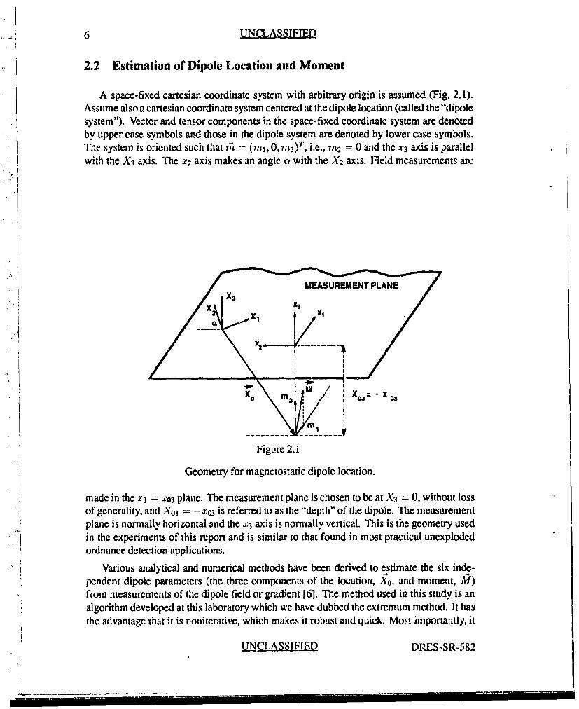
A space-fixed cartesian coordinate system with arbitrary origin is assumed (Fig. 2.1).Assume also a cartesian coordinate system centered at the dipole location (called the "dipolesystem"). Vector and tensor components in the space-fixed coordinate system are denotedby upper case symbols and those in the dipole system are denoted by lower case symbols.The system is oriented such that ri = (mj1, 0, m 3)T, i.e., mn2 = 0 and the X3 axis is parallelwith the X3 axis. The x2 axis makes an angle a with the X2 axis. Field measurements are

I I

- ------------- I

Figure 2.1

Geometry for magnetostatic dipole location.

made in the X3 X03 plaue. The measurement plane is chosen to be at X3 = 0, without lossof generality, and Y03 -x03 is referred to as the "depth" of the dipole. The measurementplane is normally horizontal and the X3 axis is normally vertical. This is the geometry used"in the experiments of this report and is similar to that found in most practical unexplodedordnance detection applications.

Various analytical and numerical methods have been derived to estimate the six inde-pendent dipole parameters (the three components of the location, XC0, and moment, MJ)from measurements of the dipole field or gradient [6]. The method used in this study is analgorithm developed at this laboratory which we have dubbed the extremum method. It hasthe advantage that it is noniterative, which makes it robust and quick. Most importantly, it

UNCLASSIFIED DRES-SR-582

,UNCLASSIFIED= 7'-I

is the only noniterative algorithm for a generally oriented dipole which can use input datafrom a total field magnetometer. The algorithm is outlined below and is described in detailin [10].

If both a maximum and a minimum of a field quantity can be found in the plane ofmeasurement, six independent pieces of information are available and the dipole parameterscan in principle be determined. Bj has more than one extremum and hence is a candidatefor such a method. B3 is not itself a rotationally invariant quantity. However, if the anglebetween the normal to the measurement plane and earth's field direction is <-, 15 -200 (e.g.,high to mid-latitudes), the 3-component of the secondary field is reasonably approximatedby (Bt - Bo) (Equation 2.2) and hence B33 -,an be measured by a total field magnetometerwhich is insensitive to orientation. Note ,nat the angle in question at our laboratory site is170.

It can be shown [101 that the positions (x',, x) of the extrema of B3 in the measurementplane are given by

S= fj(/3)X0 3 ; x• 0 j = 1,2,3 (2.4)

where f1 are monotonic analytic functions of 3 = mI /m3 whose ranges are 2 < f1< oo,0 < f2 • 1/2 and -2 < f3 < -1/2. The positions of the extrema lie in the plane alonga straight line which coincides with the X2 axis. (An exception is the case of a verticaldipole for which choice of X2 axis is arbitrary. A maximum exists immediately above thedipole and a continuous ring of minima is centered on the maximum.) Thus, the angle awhich relates the orientation of the dipole coordinate system to the space-fixed system isimmediately known once the positions of the extrema are found. It turns out that j = 2corresponds to a field maximum 3 , while j = 3 is a field minimum Bin and j = I isa saddle point. The field values at the maximum or min,;mum are given by

B3 = 47r-Mr-1 ( 1 (I+ f) 3 2 -1 + 3 (1 + ± )- (1 + 13f 3)] (2.5)

where m = v/U-• and j = 2 (maximum) or 3 (minimum),

The ratio of the field minimum to the field maximum is a monotonic function of 3 whichcan be inverted by approximating the function for intervals of /3 by polynomials of the form

k=O

where ajk are the fitted coefficients for the jth interval of 3. Three intervals with 3 <n < 6 for each interval have given very accurate approximations to the function. Thecorresponding coefficient'; are given in [101.

The algorithm, then, is simple to implement. First the space-fixed coordinates of theposition in the measurement plane of the maximum and minimum (X'j, Xzj) are foundand a is estimated. The differences in x, coordinates between the maximum and minimumare obtained by a simple rotation transformation using cr. Next, 3 is deduced from themeasured ratio of field minimum to maximum by Eq. 2.6 and is used to estimate f2, f3.

DRES-SR-582 UNCLASSIFIED

-'•, -•'-. ,--------- ---- ....... ) .. . . .•-- "• " . ..... .i i'

8 UNCAS ED

Estimates of f2, f3 and the differences in xi coordinates of maximum and minimum areinserted in Eq.2.4 to estimate X03. The x, coordinates of the maximum and minimum arenext calculated using Eq.2.4 and are used to find X01, X02 from,

X01 = - x cosa • X2 •= X -j i (2.7)ij I Il -x j sin

where j = 2,3. The position X-0 is now known and since P, a are known, the direction of

M is completely specified. Finally, m, the magnitude of M, is obtained from Eq.2.5.

Small modifications to the algorithm as desciibeoi are necessary for the case of a verticaldipole, and some heuristics are used to handle minima that are too small to be observed[10].

2.3 Identification of a Spheroid From Its Dipole Moment

The previous algorithm can estimate the locati" ui and moment of the dipole associatedwith a compact ferrous object. However, it is the location and identity of the compactferrous object that is required. Six parameters uniquely define - dipole source, but withthe exception of the sphere, more than six parameters are needod to ;-pecify the compactobject. This means that if field measurements are made at suficint distance from a sourceso that higher order multipoles are negligible with respect to the diplle, one cannot ingeneral distinguish between two compact orientable bodies. Information is necessary fromhigher order multipoles if the problem is to be have a unique inverse. Estimation of thesemultipoles is difficult, usually relying on fitting the field to a source model and solution isdependent on the shape of object.

Fortunately in practical applications there are usually a small number of object shapesand sizes applicable to a particular problem. If the dipole field associated with each objectof the set is sufficiently different from that of the other objects, identity can be reliablydetermined from the dipole field. We will now outline the method that is used by the smartmagnetometer to identify compact ferrous objects based on their magnetic dipole moments.It employs a novel pattern classification technique which is discussed more fully in [11].

It is assumed that we have determined the location and dipole moment components ofthe object relative to a space-fixed catdesia o fo..i.ate system by the . ethod de-c-r---edin Section 2.2 and that the dipole location is at or near the geometric center of the object.The latter turns out to be a reasonable assumption (see discussion of the sources of dipoleparameter estimation errors in Section 5.1). The plan is to use a pattern classificationapproach by which an object under scrutiny is identified by comparing a vector composedof features ("test vector") with feature vectors from a set of known objects ("design set").The feature vector chosen will be the dipole moment vector.

The space-fixed components of the dipole moment induced in a homogeneous, perme-able, axially symmetric, compact object by a uniform, static external magnetic iield willvary with the orientation of the object. Since two angles define the orientation, the locus

UNCLASSIFIED DRES-SR-A82

I-

UNCLASSIIED 9

of all possible dipole moments for such an object is actually a two dimensio.nal surface ina three dimensional space. (The dipole moment is usually independent of the magneticpermeability of a ferrous object in the earth's field and so only one surface exists for eachunique object shape and size.) For a spheroid, which also has Fore-aft symmetry, uniquevalues of the space-fixed magnetic dipole moment M occur only for the following rangeof the two continuous orientation parameters (0, 0) (0 = = 0), (0 < 0 < 7r/ 2 when0 < 0 < 27r) and (0 = 7r/2when0 < 0 < r).

Assume that a design set of dipole moments, Mi,k, have been niasrced at dis&ceteintervals (0j, q01) over the range of angles for which unique values of M occur. Considerthe region of the dipole moment surface corresponding to class i for which 0j < 0 < 5j+Iand ,k- _5 0 •< Ok+l. This region of the surface may be approximated by two triangles. Onotriangle passes through points Mik; Mj+i,.; M3,k+l (index i is suppressed) and is bouadedby u j,k, Tj,,and lj,k - v.,k, where

Uj,k = •41 - MIk , i,k = Mj+,,k- A1i,k. (2.8)

The other triangle passes through points M,+I,k; M1 I+,k+,; M,,k+, and is bounded by aU,k.

and k where

k u+I,k - +,,k+ wkh Ak+1 -

If -;is a test vector (suppressing subscripts j, k where unambiguous to do so), then

j= - A1,. (2.10)

If p(-) is he projection of g onto the unprimed triangle, a Gramn-Schmidtconstruction gives

= Pi,J,ki - qi,i,kV (2.11)

where Pij,k, qi,j,k are scalars given by

_ (pV~j (j~j7 - ("~7 (iT~)_ (T -) -q (U Tly)

, (vT 4v) (ff') _ (1v'7-)2 Pi,j,k - (0f 2.2

If i7 is a sample from the class i corresponding to the region of the dipole nmument surfacebounded by il, it- - 67, then estimates, 0 and q, of the continuous parameters associatedwith x may be obtained from

O=O + qgj,k (Oj+l 0.) , (2.13)

Ok + p,,k (O+l - OJ ). (2.14)

DRES-SR-582 UNCLA 1SIFIED

10 UNCLASSIFIED

The minimum distance, dij,k, from the test vector to the triangle is given by

d= ; = (TJ/ (2.15)

The previous equations give the minimum distance to the triangle if WO) lies within theboundaries of the triangle. This is true provided p,j,, > 0, q,, > 0 and 0 < Pij,k + qij,k <S1. If these conditions are not satisfied, then di,.,k is replaced by the minimum distance fromthe test vector to the line segments which bound the triangle.

A similar process is applied to the primed triangle, yielding a minimum distance d'The minimum distance, d,, from the test vector to the class i dipole moment surface is thenapproximated by

di = min {di 1j.k, Id,j,k (2.16)j,k

The dipole moment surface for 0 = 0 is independent of 0. In this case, the manifoldhetween 01 =zO, 0, 01 , and qOk1+ is approximated by a single triangle connecting Mk,PA11+1,k ,A'I+1,k+..-

This classification method has been tested on a design set consisting of noise-freemagnetic moments for six different spheroids, typical of the size and shape of a widevariety of artillery shells (0.01 < a < 0.09 m, 2.5 < e < 3.75, where a, e are defined in'1 Section 2.4). These were computer generated at 150 increments of the orientation angles0, q0. Test vectors were computer generated at 50 increments with additive Gaussian noiseof different levels. The probability of misclassification was about 1% for noiseless testvectors, 3% for moments with noise which was 5% of the moment component value foreach component, and 7% for moments with 10% noise [I11].

The identification method has been presented for a compact axially symmetric object

but can be generalized to a compact body of arbitrary shape [11].

2.4 Multipole Expansion of the Magnetic Field of a Spheroid

In this Section, we present a mathematical model for the magnetic field induced in ahomogeneous spheroid of arbitrary orientation by a uniform magnetostatic field. The modelcan be used both to develop a design set for use by the magnetometer's pattern classifier (see

• ,•:"[previous Section) and to provide controlled magnetic field data for analysis of the location

estimation algorithm error. The model has been shown to provide magnetic fields that are agood approximation to those of real spheroids and some unexploded ordnance in the eart.h'sfield [7], [8]. A brief outline of the model is given below. A detailed derivation may befound in [9].

It is assumed that a homogeneous uniformly permeable spheroid, with magnetic perme-abilityu,• •o and no permanent magnetization, siL:; in a homogeneous surrounding medium

i TCLASSIFIED. DRES-SR-582

UNCLASSIFED 1

with permeability ji,2po, where po is the permeability of fre space (Fig. 2.2). There

X 3

\ i " k -~ ~~. J.. . . . . . . .SSYM Y AXIS

ii , /

Ir 2

x 2

X3

Figure 2.2

Geometry for calculation of the magnetic field of a spheroid.

exists a uniform parallel external magnetostatic field. A body-fixed cartesian coordinate

system whose 3-axis coincides with the symmetry axis of the spheroid, has an origin at thegeometric center of the spheroid. There is also a space-fixed coordinate system to whichmeasurements are referenced. Without loss of generality, the space-fixed system is chosen

so that the primary magnetic field, Bo, has no 2-component, i.e., B0 = (Bol, 0, B0 3 )T. Thespheroid center is located at Xo = (Xo1 , X 02 , X03)" in this system. Vectors are indicated bylower case letters in the body-fixed system and upper case, letters in the space-fixed system.The angle between the spheroid symmetry axis and the X3 axis is 0. The angle betweenthe projection of the symmetry axis on the horizontal plane and the X, axis is 0. It canbe shown [12] that the induced field, and hence the magnetization, inside the spheroid isuniform and parallel. By carrying out a multipole expansion of the static field, and with theassumptions of uniform parallel internal magnetization, it may be shown that the secondaryinduced magnetic induction measured at a point i-" = (XI, X2, x3) in free space, complete tofourth order, is given by 19] 1

b-- b(2) +±M8 ) (2.17)

where b( 2) is a dipole field term and b(8) is an octupole field term. The two field terms may

DRE-S-SR-582 UNCLASSIFIED

12 UNCLASSIFIED

be expressed in component notation using summation convention as6() MO)..3 + 3r 2 (2.18)

4 [XiOm16IX)]

and

b -- r 5 "(3Or n - 15r-2 [x'xpm (3 + xjx.,r ] +(35r -4Xryx'M(3)

(2.19)where m() is the dipole moment vector, and m0 is the rank 3 octupole moment tensor.Note that there is no monopole field term, as expected, and that the quadrupole term ismissing. The disappearance of the latter and, in fact all even multipole moments(m(2n)n an integer), derives from the restrictions on the magnetization of the body, M', togetherwith the axial and fore-aft symmetry of the spheroid.

The dipole moment is given by"42-) M,,V a• = 1,2,3 (2.20)

where V' is the spheroid volume. For the octupole moment tensor, only 10 of the 27elements are independent and axial symmetry reduces that number to 6. These are

M(') 31n(') - 3M'III ; () - 3m113 3Ml'I I, ; '" = 3 33"111t = 3 221 - 1 t222 - 1 3

Tr () M (3) Mi It - n() M,'13 ; {3) '3

13- rn2 - , 3-" ; r3 M3 3 332 I M (2.21)

whereI J" (r -r_ 42) dv' 13 J dv' (2.22)

Note also that(3) (3) (3)

Ma#= =ai Mlo (2.23)M (3) = 0 if a :f/ -# (Y# . (2.24)

The analysis to this point applies to any axially symmetric body with fore-aft symmetry.We now assume that the body is a spheroid whose symmetry axis length is 2ae and whosemaximum diameter orthogonal to the symmetry axis is 2a. It is simple to show that

V1=4 7re 3 w 47rC3sa5'.5V' = .reIa I ;I i = ca ; 133 = -15ea (2.25)

Assume that the external magnetic field (usually the earth's) in the absence of thespheroid is b = (bo0, b2. b03) . A solution of the boundary value problem vields [121

Mi = P _bo j P 1,2,3 (2.26)

The demagnetization factors F/ are given by

S(pL,, - 1) / (1 + A, [Ari - Pr2J / [2/421) (2.27)

UNCLASSI IFID DRES-SR-582

I I II I II

UNCLASSIFIED 13

A= A2 e(e + E) (e2 -1)1I A3 =-2e (e1 - E) (e2 1)- (2.28)

E = In (e- [e2- 1]•) (e2 - fore > I (prolate) (2.29)

E =(arctan I - e2-]- 7r/2) (I- for e < 1 (oblate) (2.30)

2A,=A2 =A 3 =2 fore=I (sphere) (2.31)

3

Field quantities have been derived in the body-fixed coordinate system whereas quanti-ties are needed in the space-fixed system in which measurements are made. A body-fixedvector t7 and its related space-fixed vector U are connected by the relation

i= AO (2.32)

where A is the well known Euler rotation tensor corresponding to Euler angles (0b, 0, 0).

Equations 2.17 through 2.32 allow one to calculate the magnetic field B at a point inspace due to the presence of the spheroid, given the size and shape of the spheroid (a, e),the magnetic material properties of the spheroid and the surrounding medium (ILj, /12),

the location of the geometric center of the spheroid Xo and the orientation of the spheroid'ssymmetry axis with respect to the space fixed system (0, 0). However, the equations areinsensitive to (14i,, /r2) provided Ul /,U,2 >- 100. This is generally the case for ferrousmaterials in the earth's field. For all model calculations done in this study, we have chosena,, = 1000, /,u2 = 1, which are typical values encountered in practice.

In addition, Equations 2.20 and 2.26 through 2.32 allow the dipole moment of thespheioid in the space-fixed cartesian frame M = (M1 , M 2, M3 )T to be calculated as:

V {F I+ [P' - Fi] sin 2 Ocos 2 01}30 + {[F 3 - F,]cosOsinOcos }B3).({[1' - F1]sin 2 OcossinqS}Bo + {[F 3 - P ]cosOsinOsinq,}Bo3 .

0 {[F]- "]cos0sinOcos1•}B 0 o- + {IP + [F•- 2 ]co 2 R},,,(2.33)

DRES-SR-582 UNCLAISSIFIED

S14 IN_{C LASSRIED

LNCL~S1EiLLŽDRES-SR-582

UNCLASSIFIED 15

3. Experimental Method

3.1 The Smart Magnetometer

To obtain magnetic data as a function of position in a plane, a novel instrument has beendeveloped, which has been dubbed the "smnart magnetometer". It collects simultaneousmagnetic and position data and estimates location and identity of compact, axially symmet-ric, ferrous objects. The instrument is self-contained and can be used in a person-portableor vehicle-mounted role.

The second generation of the instrument was used in this study. It is shown in Fig. 3.1.

The major components are a total field magnetometer, a tricycle cart which holdsthe magnetometer sensor head and has a front wheel-mounted shaft encoder serving as alinear position sensor, a Motorola 68332 EVB microcontroller, an interface between themagnetometer and position encoder signals and the microcontroller and a lap-top computer.Power to the entire system can be supplied by the magnetometer battery pack, but forconvenience during the many experiments described here, a DC power supply was used.Interconnections between the electronic components is shown in Figure 3.2, while detailsof the smart magnetometer interface are shown in Figure 3.3.

A model V101 self-oscillating cesium vapour magnetometer, made by Scintrex, Con.-cord, ON, Canada, is used to obtain the magnetic data. It has a precision due to quantizationerror for a given sensor head orientation of +0.1 nT over a nominal range of 20000 nT to100000 nT The accuracy, limited by heading error, is a function of the relative orientationof sensor optical axis and ambient field direction. It is no worse than ±0.5 nT.

The magnetometer takes 45 ms to make a field measurement and provides a digital

BCD output that is updated every 89ms. The magnetometer output is buffered and fedto parallel digital input ports of the microcontroller. As well, the two phase outputs fromthe position encoder are fed to the input of an advanced timer/counter unit (TPU) on themicrocontroller. The pcsition encoder interrupts the microcontroller and increments ordecrements a register 2Wd0 times for each revolution of the front cart wheel. (The TPUcompares the relative phases of the encoder signals to determine the direction of motionof the wheel and correspondingly increments or decrements the register.) The wheelcircumference of 0.618 m then corresponds to a limiting positional resolution of 0.309 mm.However, the effective resolution is governed by the magnetometer field measurement time,

DRES-SR-582 UNCLASSIFIED

16 UNCLASSIFIED

Figure 3.1

Second generation "smart magnetometer". The tricycle cart is on theleft. The position encoder is attached to the front wheel of the cart. Themagnetometer consists of a display box on the right, a cylindrical sensorhead which is attached to the main rod of the cart and an amplifier andsignal conditioning unit and battery pack which are not visible. The laptop computer is in the center of the photograph, but the microcontrolleris hidden from view.

UNC. A... _I DRES-SR-582

_.... . ... .. . ;- I"....-

.. .. . .,-Z•• " •'• , ,,• • . .

Magnetometer Amplifier andSenseHeaSignal Conditioning

Control Box

Smart Magnetometer Block DiagramFigure 3.2

Electrical connections between components of the smart magnetometer.

DRES-SR-582 1)NCL.AS FIED

18 UNCLASSIFILE

MosIW 36 P- . SIZI

Sig. 3 ,5 - .- ±i- AS

Digit 34 P4-7 DS

74HC S418P4-5 CL. M

3 P4-4 AVEC5 P5-11

-- DSACK1

I P6.121 _- _J DSACK0

---.- P6-10 - R064 P6-9

-0- -O QRO56 -0- P6-7 IRQ4

-lb -0- -* R0319 74H 1 P6-6

10 -0- P6-5 IRO2

37 P6-190 -" S-b -MOSI9 MIS a MISO

18 P6-16-. D-- m PCS3

11 P6-15Least o1w15 PCS2Sig. IsPS.14-

14g. 15 -PCSL~iGC -4 •;P7_ j SCK

74HC541Data Strb. 23 0- _ _ -.. P2-19 TPO

Magnetometer

Phase A P2-15 - TP4Phase B JP2-6 TP3

Optical Encoder 68332 EVB

Smart Magnetometer interfaceFigure 3.3

Smart magnetometer interface. Interface buffers signals between themagnetometer and position encoder on the left and the microcontrolleron the right. Magnetometer and microcontroller signal names are" thoseused by their respective manufacturers [131,[141.

UNCLNASSIFIED DRES-SR-582

UNCLASSIFIED 19

since the magnetic field value is uncertain within this time period. The effective positionalresolution in the direction of motion is thus dependent on cart speed and is I 125 cm at0.25 m/sec and 1.350 cm at 0.30 m/sec. The software running on the microcontroller readsthe magnetic field ports, converts the values to a magnetic field and then reads the positionregister whenever the magnetometer outputs a new value. The magnetic field conversiontime is less than the spacing between encoder interrupts (-- 1 msec at 0.3 m/see) and so theposition value corresponds to the position at which the magnetometer signalled that it had.acquired the magnetic value. The magnetic field value and the current position value arestored if a predetermined distance has been spanned since the last update.

The microcontroller is the heart of the instrument. It controls collection of magneticN.. and position data and algorithm execution. The menu-driven software has the followingmodes:

* Free running - Gives bar graph indication of field strength. Allows the operator tofind regions which have magnetic field values of sufficient strength and spatial extentto warrant further investigation.

e Locate - Instructs the operator when and where to make magnetic field and positionmeasurements. Estimates location and moment of the dipole associated with adetected object from the field measurements using the noniterative algorithm ofSection 2.2.

* Identify - Identifies detected object from its dipole moment, estimated from the"Locate" mode, using the pattern classifier of Section 2.3.

9 Design set update - If the identification was carried out on a known object, this modeuses the results to modify or add a feature vector to the design set.

o Magnetic map transfer - Allows magnetic maps to be transferred to the lap topcomputer hard disk.

e Design set transfer - Allows design sets to be transferred to/from the lap top computer

hard disk.

The lap top computer is initially used to down load code to the nmicrocontroller and acts

as a file server for magnetic/position data and design sets for experimental purposes. Inan fielded instrument, code can reside permanently on the microcontroller EPROM and thelap top can be replaced by a hand-held terninal or notebook computer.

The location algorithm execution time is a function of how finely the field is sampledin the plane above the object of interest because this determines how many magnetic datavalues must be searched to find the extrema positions. The location algorithm executed infive seconds for a 170 cm (--.2 cm sample increments) by 210 cm (5 cm sample increments)grid (,-- 38(X) total data points in the magnetic map). Execution time for the identificationalgorithm, which is itidepcndent of magnetic map size, took about 30 seconds for a 6 object

DRES-SR-582 U)NhCLASSIFIED

20 UNCLASSIFIED

design set. These times are still small compared to the data collection time. It took 6minutes to collect the data for a 170 cm (-•2 cm sample increments) by 210 cm (10 cmsample increments) grid and 13 minutes for a 170 cm (-,-2 cm sample increments) by 210cm (5 cm sample increments) grid.

3.2 Experimental Layout

Measurements were made in the Threat Detection Group's nonmetallic laboratory whichhas been described in detail in [7]. The laboratory is a 12 m diameter hemisphericalnonmetallic building with minimal metal content. Magnetic field gradients are typically nogreater than I or 2 nT/m in the usable portions of the building. Magnetic field fluctuations-are limited by geomagnetic noise and were typically ± 1-2 nT/hour during the time of dayin which measurements were made (mid-.morning, early afternoon). In the time necessaryto measure a magnetic field map (- 15 minutes or less), background noise fluctuations wereless than the quantization error of magnetic data received by the microcontroller (1 nT) andthus no reference magnetometer was used for background subtraction. The experimentalset-up is shown schematically in Fig 3.4.

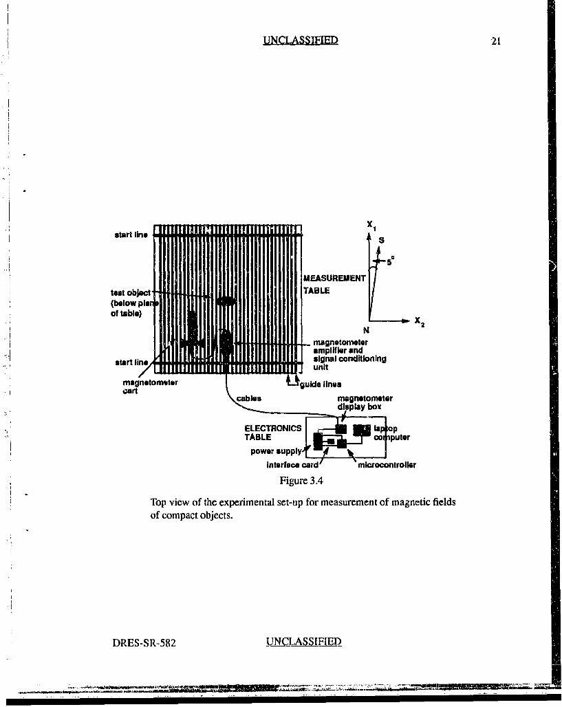
The measurement table on which the magnetometer moves was situated in a low gradientpart of the laboratory. The table was made of wood with brass screws and was heavilyreinforced to ensure negligible displacement of the measurement surface when walked on.The horizontal measurement surface was 3.66 m on a side and was 1.04 m above the floor.The table surface was painted in alternating light and dark coloured guide lines spaced 4.8cm apart. The table was oriented so that the guide lines ran along a direction 50 from anorth-south direction (Fig. 3.4). This direction was labelled X1. The horizontal directionorthogonal to the A)1 direction was labelled X2. A start line, parallel to the X2 direction,was situated at either end of the table. Because of practical considerations such as the finitesize of the magnetometer cart, placement of the start lines and positioning of the operator,the usable region of the measurement surface was about 2.7m in the X, direction and 2.55min the X2 direction. The intersection of the lower start line and the left-most guide linewas considered to be (0,0, -0.24m) in the space-fixed coordinate system since the nominalcenter of the magnetometer active volume was 24 cm above the table surface.

The object of interest was placed in a wooden holder that allowed the object to be rotatedindependently about a vertical or horizontal axis and locked at a desired orientation. Thegeometric center of the object of interest was then placed directly below the center of themeasurement table at a variable depth and orientation. The orientation of the object wasdefined by two angles. The polar angle, 0, was the angle between the X3 (vertical) directionand the symmetry axis of the object. The azimuthal angle, $, was the angle between thenorth-south direction and the projection of the symmetry axis on the X, X 2 (horizontal)plane.

A separate wooden table, on which the electronics was placed, was situated roughly 2in from the measurement table. Although all of the electronics could have been carried by

UNCLASSIFIED DRES-SR-582

UN~CLASSIEIED 21

........... X lstart line

test object . ..... ... A L(below plan

*rof table)

.. .....tomntoterestartI. W 1 ui

mmagnetometer

cartFigurde 3.4ec~a W amagatorstITop vew ofthe eperimntal etupforpmasuemn bofx antcfed

ofCTONC comac objcts

DRES-TABLE 0N(1LASSIF1E

r

22 UNCLASSIFIED

the operator, it was felt better for experimental purposes to keep the cormponents separatefor ease of modification and to keep them distant from the measurement surface to ensurethat stray magnetic fields from the electronics would not interfere with the magnetometersensor. Because of cable length restrictions, the magnetometer electronics box was kept onthe measurement table approximately 0.5 m from the magnetometer cart.

3.3 Procedure

1b collect a magnetic map the following procedure was used. Prior to collecting theinitial map, the electronics were connected, powered up and allowed to stabilize for at leastten minutes. The operator removed all metal and placed it far from the measurement table.The microcontroller code was downloaded from the lap top computer and the program wasinitiated. For all maps, the object of interest was placed in the appropriate position andorientation. The magnetometer cart was positioned with its rear wheels at the lower startline and its front wheel on the left-most guide line of Figure 3.4 (cart pointing in the positiveXT direction). The "Locate" mode of the software was selected and initial parameters wereentered (XI, X2 maximum dimensions, sample spacing). The background magnetic fieldwas sampled for approximately 2 seconds and then a tone signalled the operator to roll thecart with the front wheel running along the guide line. Data would not be collected untilthe wheels started to roll. While rolling, simultaneous magnetic and position information

were automatically acquired. When the microcontroller sensed that sufficient distance hadbeen traversed, data collection was halted and the operator was signalled to stop. The set

of position and magnetic data collected along a guide line is called a "scan" or a "scanline". The operator then sct the cart with its rear wheels at the upper start line and its frontwheel on the next guide line in the positive X2 direction (cart pointing in the negative XAdirection). The software had a built-in delay during which data collection was suspendedto allow such positioning of the cart. The microcontroller would then signal the operatorto commence rolling the cart. (Note that the microcontroller software can use the wheelposition encoder to guide the mtagnetometer to the start of the next X, scan. This is notas accurate as using well defined guidelines and starting points and so this feature was notused for these experiments.) The procedure was repeated and a two dimensional array ofmagnetic values versus A 2 I, X2 (whicll" " Wb•, caltd a magnctic mnapl was acqumr,,. In araster scan fashion until the microcontroller signalled the operator to halt. The locationof the object and its associated dipole moment were then estimated and the object was

classified. If desired, magnetic data were transferred to hard disk for permanent storageand then the prt(cedure was repeated for a new map.

3.4 Initial Calibration

Prior to commencing the location and identification experiments, a number of magneticmaps were collected to optimize operational procedures and parameters. Yawing of the

VLNCLAS F I-IED DRES-SR-582

L UNCLASSIFIED 23

seisor head was initially noted as a problem, as was an offset between the magnetic sensor,ead path and the encoder wheel path. Both of these were remedied by modifying the cart.

Optimum scanning spead for the sensor was determined. Because of the fixed temporalspacing between magnetometer outputs, the cart speed had to be adjusted so that the sample

* spacing was not too large, while still quickly completing a scan. A sample spacing of about2 cm was desired. It was found that a reasonable sensor speed was roughly 0.30 to 0.25rm/sec. The cart would require 8 to 10 seconds to move from start to finish of one scan lineand the microcontroller would store a magnetic field reading every 2.2 to 2.7 cm along theX1 direction.

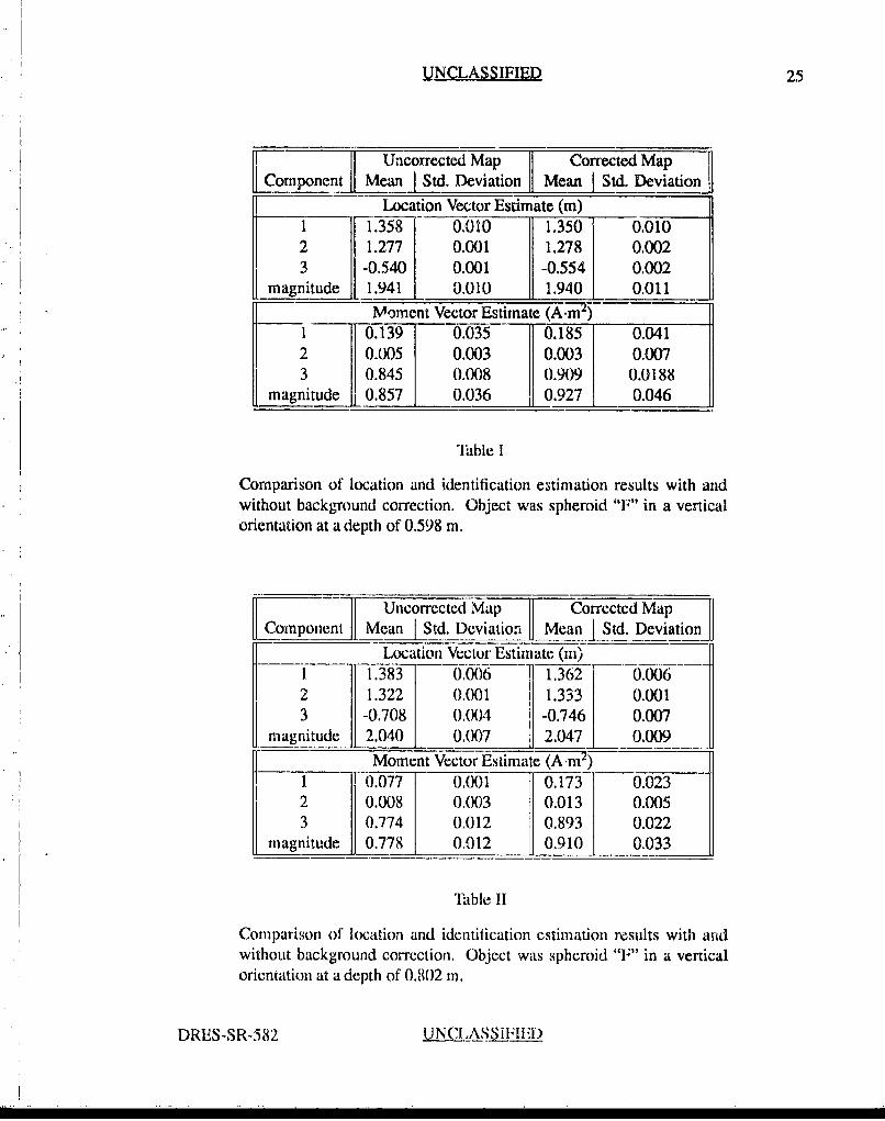
A magnetic map was obtained with no object in place, in order to measure the back-ground magnetic field. The map is shown in Figure 3.5. The field gradient is seen tobe roughly constant and can be characterized by a single component pointing from thenortheast to the southwest corner of the table with magnitude - 2 nT/m. The effect ofthe background is small but significant, particularly for the momer~t estimation when themagnetic field of the object is weak. T1ypical examples of the difference in estimation withand without background subtraction are shown in Tables I and II. The object was spheroid"F" (see Table IV for description) in a '.'ertical orientation at depths of 0.598 m (Table I)and 0.802 m (Table 'if). Peak field value due to the object was ,-. 10OOnT for Table I and- 350nT for Table II. For both Tables, the sample spacing in X2 direction was 4.8 cm.Seven field maps were used for estimation. Standard deviation for the magnitude is actuallythe root average square distance (inutaset distance) between vectors, based on 7 field mapsfor Table I and 3 field maps for 'fable II. The difference in estimates between correctedand uncorrected maps is at most only slightly greater than can be accountedt for by thestandard deviations for the 0.598 m depth. The difference becomes significantiy greaterthan the statistical uncertainty at a depth of 0.802 mn, which is to be expected because of thediminished field due to the object.

In the experiments that follow, the background map was subtracted from the magneticfield map due to the object before applying the location and identification algorithms.

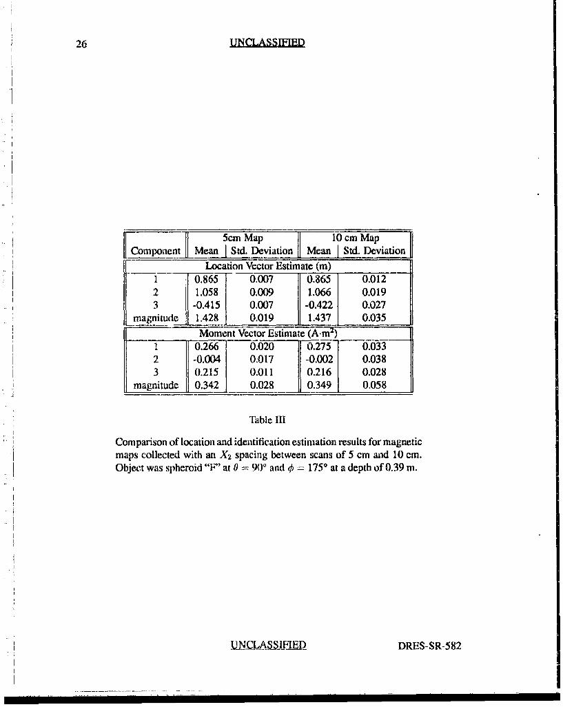
The measurement table guide lines would allow scan lines a.; close together as 4.8 cmor at any multiple of 4.8 cm. It was desirable to use the closest spacing possible for thestudy of the location algorithm, but it was necessary to know how sensitive the algorithmestimates were to the X2 spacing. To test this sensitivity, a set of measurements were madeon a fixed object at a fixed orientation. The depth chosen was small (039 m) since theestimation should be more sensitive to grid spacing when field maps are narrow as they areat shallow depths. The results are shown in TablellI, The object chosen was spheroid "F"(see Table IV) at 0 = 900, g = 175' and at a depth of 0.39 m. Five field maps were usedfor estimation of 5 cm spacing data and two field maps were used for estimation of the 10cm spacing data. (These data were obtained on an older, smaller measurement table whichhad a minimum scan line spacing of 5 cm, rather than 4.8 cm.) The standard deviation forthe magnitude is actually the root average square distance. Clearly, there is not a significantdifference between the two spacings.

DRES-SR-582 LIN.' ,ASSIFIED

24 UCLASSIRIED

Bockground on Big Toble 16/07/92 PM8 backqround.dat

6

I H--c 4

2

* Figure 3.5

Background magnetic map collected by the smart magnetometer on themeasurement table surface.

V-N-QA-ýSI F IED DRES-S"-.-582

©I

UNCLASSIFIED 25

Uncorrected Map Corrected Map[Component Mean__ Std. Deviation I Mean I Std. Deviation]

Location Vector Estimate (m)1 1.358 0.010 1.350 0.0102 1.277 0.001 1.278 0.0023 [-0.540 0.001 -0.554 0.002

magnitude 1.9411 0.010 1.940 0.011Moment Vector Estimate (A-m-7- -

0.139 0.035 0.185 0.0412 0.005 0.003 0.003 0.0073 0.845 0.008 0.909 0.0188

magnitude 11 0.857 1 0.036 0.927 0.046

"Tlble I

Comparison of location and identification estimation results with andwithout background correction. Object was spheroid "F" in a verticalorientation at a depth of 0.598 m.

Uncorrected Map i Corrected Map

Component Mean I Std. Deviation Mean Std. DeviationLocation Vector Estimate (m')

1 1•383 0.006 1.362 0.0062 1.322 0.001 1.333 0.0013 -0.708 0.0X)4 -0.746 0.007

magnitude 2.0401 0.007 2.047 0.009Moment Vector Estimate (A m _)

1 10.077 0,001 0.173- 0.0232 0.008 0.003 0.013 0.0053 0.774 0.012 0.893 0.022

magnitude _0.778 0,012 0.910 0.033

"Table II

Comparison of location and identification estimation results with aridwithout background correction. Object was spheroid "F" in a verticalorientation at a depth of 0.802 m.

DRES-SR-582 _UNLASSIF IFD

26 UNCLASSIFIED

Comonet M an c Map Ma 10 cm MapComponent Std. Deviation anStd. Deviation

Location Vector Estimate (m)

1 0.865 0.007 0.865 0.0122 1.058 0.009 1.066 0.019

_3 -0.415 0.007 -0.422 0.027magnitude 1.428 0.019 1.437 0.035

Moment Vector Estimate (A-m2 )_ _

1 o0.266 0.020 0.275 0.0332 -0.004 0.017 -0.002 0.0383 0.215 0.011 0.216 0.028

magnitude 0.342 0.028 0.349 0.058

Table III

Comparison of location and identification estimation results for magneticmaps collected with an X2 spacing between scans of 5 cm and 10 cm.Object was spheroid "F" at 0 WYl and q 1750 at a depth of 0.39 m.

UNC. UAFLFFŽ DRES-SR-582

" • I • • I I II

]dFAS SIFIED 27 m-

4. Experimental Results

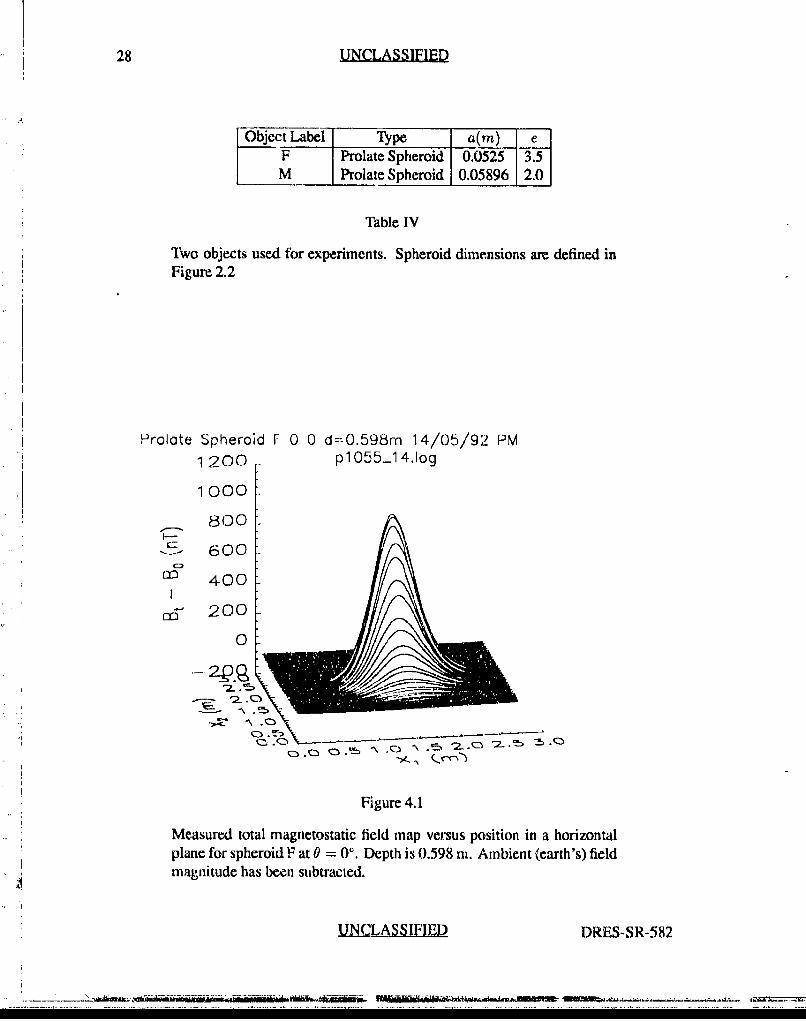
Using the experimental method of the last Chapter, magnetic maps were obtained fortwo mild steel solid spheroids for a variety of depths and orientations. The two objectsare summarized in Table IV. Both objects are typical of the size and shape of unexplodedordnance. In the following discussion, the type of spheroid and its orientation for a particularexperiment will be designated by a letter (assigned for historical reasons) and two integers.For example, M 90 175 refers to the type "M" spheroid with a polar angle of 90' andazimuthal angle 175*. The orientation for a vertical spheroid is denLced 0 0, even thoughthe azimuthal angle is, strictly speaking, undefined. The orientation angles are defined inSection 3.2.

Figures 4.1 to 4.4 are typical of the variation of magnetic field maps for a single objectfor different orientations. Both the maximum field value and the relative position of themaximum and minimum field value change with orientation. The maximum field value isseen to decrease with increasing polar angle. This illustrates that simple location schemeswhich assume that the object center is directly under the maximum field position will haveserious errors as will simple identification schemes which use only the maximum ficld valueas a feature.

The location estimates for all experiments are given in Table V. The dipole momentestimates for all experiments are given in Table VI. For both tables, where multipleexperiments were done for identical conditions, the standard deviations are given. Notethat the range of depths is from 0.39 m to 0.802 m. The lower limit was mainly imposed bythe measurement table surface thickness plus magnetometer height plus minimum objectdimension ( 4 + 24 + 10.5 cm respectively), while the upper limit was set by therequirement to havea suffilctie signai-to-noisc iatio (SNR) to gei reasonable precision forthe spheroids studied.

It is necessary to characterize both the precision and the accuracy of the locationalgorithm. To determine the precision or repeatability, one can look at the location anddipole moment estimates for independent magnetic maps that were obtained for the sameobject, orientation and depth. Precision of a location vector component was measured by thestandard deviation of the component, expressed as a fraction of the depth, while precisionof a moment vector component was measured by the standard deviation of the component,expressed as a percentage of the average magnitude of the vector. A good measure of thedeviation of vectors sampled from the same population is the intraset distance. Given a set

DRES-SR-582 VQNLASIFF.ED_

28 UNCLASSIFIED

Object Label Type a(m) eF Prolate Spheroid 0.0525 3.5M Prolate Spheroid 0.05896 2.0

Table IV

Two objects used for experiments. Spheroid dimensions are defined inFigure 2.2

Prolate Spheroid F 0 0 d-O.598rn 14/05/92 PM1200 p1055-14.log

1000

800

-- 600

r• 400

S200

0

' .- Z . '

-.• .,-- -,,

Figure 4.1

Measured total magnetostatic field map versus position in a horizontalplane for spheroid F at 0 = 0'. Depth is 0.598 m. Ambient (earth's) fieldmagnitude has been subtracted.

UNCLASSIFIED DRES-SR-582

UNLAj&E= 29

Prolate Spheroid F 30 175 d=O.525m 06/08/92 PM1.500- oug6_2,dot

1000

500

OT 0

Figure 4.2Measured total ,agnetositati. field =p versus posion ir a 1-0plane for spheroid F at 0 = 30' and 1 =750. Depth is 0.525 m.Ambient (earth's) field magnitude has been subtracted.

DRES-SR-582 -UNCLASSWWJ)

30 UNCLASSIMFIE

Prolote Spheroid F 60 175 d=0.525m 06/08/92 PM1 000 -auq6_.dat

800

600F--

5- 400

c• 200

0-- 200

Figure 4.3

Measured total magnetostatic field map versus position in a horizontalplane for spheroid F at 0 = 60' and ¢ 175'. Depth is 0.525 m.Ambient (earth's) field magnitude has been subtracted.

UNCLASSIFIED DRES--SR-582

UNCLASSIIED 31

Prolate Spheroid F 90 175 d=0.655m 16/07/92 PM

ju 1 6_2.dot150

1 00

H--

o, 50050

"CO.

Figure 4.4

Measured total magnetostatic field map versus position in a hors =ontalplane for spheroid F at 0 = 900 and 0 = 1750. Depth is 0.655 m.Ambient (earth's) field magnitude has been subtracted.

DRES..SR-582 1NCLASSIFIED

32 UNCLASSIFIED

Spheroid Measured EstimatedTyro, nko, X02 IX03_ ___UXOrientation.I (m) (m), (m)I (rn, (m) (m)

FOO 0.87 1.04 0.5G 0.870 1.05 0.4111.321 1.288 0.598 1,350-±0.010 1.278 ± 0.002 0.554 1 0.0021.357 1.333 0.698 1.372± 0.002 1.317 ± 0.002 0.642 ± 0.0001.357 1.333 0.802 1.362 ± 0.006 1.333 ± 0.001 0.746 ± 0.0061.347 1.293 0.565 1.344 ±: 0.002 1.298 ± 0.000 0.487 0-.001

M 10 175 0.87 1.04 0.50 0.862 1.05 0.458F90 175 1.362 1.313 0.525 1.368 1.311 0.534

0.855 1.04 0.390 0.865 ± 0.007 1.058 ± 0.009 0.415 ± 0.0070.87 1.04 0.440 0.894 1.050 0.5041.36 1.33 0.655 1.391 1.306 0.676

F60 175 1.362 1.313 0.525 1.392 1.307 0.539F 30 175 1.362 1.313 0.525 1.405 1.301 0.494F60265 1.362 1.313 0.525 1.408 1.316 0.556F 30 265 1.362 1.313 0.525 1.389 1.326 0.499M 90 265 0.87 1.04 0.438 0.884 0.005 1.040 A: 0.001 0453 ± 0.007" 0.87 1.04 0.468 0.877 1.070 0.455

0.91 0.97 0.580 0.938 1.003 0.524

Table V

Location estimation results using experimental data from spheroids.Where multiple experiments have been done under identical conditions,standard deviations are given.

DRES-SR-582

UNCLASSIFED 33

Mathematical Model Estimated

Type. (m) (A.m2) (A.m 2) (A.m 2) (A.m 2) (A.m 2) (Am 2)Orientation l r_

I FOO 0.500 0.065 0.000 1.069 0.072 0.001 0.7160.698 0.065 0.000 1.069 0.177 0.013 0.876

_+ 0.005 ± 0.013 + 0.0010.565 0.065 0.000 1.069 0.161 -0.009 0.701

__.-_ 0.003 ± 0.001 ± 0.0020.598 0.065 0.000 1.069 0.185 0.003 0.909

±- 0.042 ± 0.007 ± 0.0190.802 0.065 0.000 1.069 0.173 0.013 "0.893

S+± 0.023 ±50.005 ± 0.022I F 90 175 0.390 0.325 -0.023 0.212 0.266 -0.004 0.215

±0.020 ± 0.017 ± 0.0110.440 0.325 -0.023 0.212 0.315 -0.001 0.2450.655 0.325 -0.023 0.212 0.238 -0.015 0.1820.525 0.325 *-0.023 0.212 0.410 -0.035 0.191

M 90 265 0.438 0.059 0.007 0.189 0.082 -0.061 0.1584- 0.006 ± 0.001 ± 0.007

0.468 0.059 0.007 0.189 0.039 0.029 0.1050.580 0.059 0.007 0.189 0.028 -0.003 0.123

F 60 17 0.530 0.621 -0.049 0.539 0.779 -0.062 0.550F 30 175 0.525 0.499 -0.038 0.967 0.554 -0.040 0.833

F 60 265 0.525 0.099 0.386 0.436 0.137 0.495 0.541IF 30 265 0.525 0.098 0.375 0.864 0.169 0.028 0.817

M 10 175 0.500 0.105 -0.004 0.455 0.030 -0.003 0.300

, "Table VI

Dipole moment estimation results using experimental data fromspheroids. Where multiple experiments have been done under identicalconditions, standard deviations are given. Theoretical moment compo-nent values are obtained from the mathematical model of Section 2.4.

DRES-SR-582 UNCLASSIFIED

34 UINCLASSIFIED

of vectors, a', i = 1, ... , K, the intraset distance, Df, is the mean square distance betweenvectors given by [15]

•-•= I K K n

D2 E l) - (4.1)K(K j=l i=1 k=1

where a' is the kth component of as and k = 1, ... n. The precision in estimation of locationvectors was taken to be the square root of the intraset distance between individual locationvector estimates for a given object, orientation and depth. For two depths, 0.500 m and0.525 m, different orientations and/or objects were used to determine the precision in depthwhereas for other depths, these parameters were constant for a given depth. The precisionin estimation of moment vectors was assigned to be the square root of the intraset distancebetween individual moment vector estimates. Since moments are a function of object typeand orientation, precision in moments could not be determined for the 0.500 and 0.525 mdepths. The results of the precision in estimation are given in Tables VII and VIII andFigures 4.5 and 4.6.

From Tables Vlland VIII and Figures 4.5 and 4.6, it can be seen that the precision inestimating location varies from 0.12 to 1.90%. However, there is also a variation in locationestimate with object type and/or orientation, since the two depths with the worst precision(1.67, 1.90%) are the only ones which have different types and orientations included inthe precision estimates. If these are excluded, the precision in depth ranges from 0.12 to1.35%. The precision in estimating the dipole moment varies from 0.51 to 8.21 %. Thereappears to be a slight increase in uncertainty as depth decreases, but the precision is notclosely correlated with the peak magnetic field. This variation in precision may be partlybecause the widths of the magnetic field maps scale linearly with depth. When samplingwith a fixed width sampling grid, estimates will be more sensitive to narrow maps. Also,the lowest depth cases were done for spheroids with a horizoitial symmetry axis. The shapeof the magnetic map for these cases will differ from those for tne remainder which are forvertical axis spheroids (compare Figs. 4.1 and 4.4). The use of a fixed width sampling gridmay then again make estimates more sensitive to one orientation than another.

It is also interesting to note that the precision of the dipole moment estimates is alwayslarger than the precision of the location estimates for the same object, orientation and depth.This is as expected, since Equafion 2.5 hows that Lo•- a giver, orientation, the mgtd ofthe moment is equal to the cube of the depth times a constant. Simple error propagationtheory then suggests that the percentage error in moment should be three times that in depth.Since error in depth usually dominates the error in the other directions [101, the percentageerror in dipole moment should be at least three times the percentage error in location.

Although the precision (repeatability) is quite good, it is also necessary tc know what isthe accuracy in estimation; that is, are the estimates biased? To get a preliminary assessmentof accuracy, the depth estimates averaged over all object types and orientations for a givendepth were plotted versus measured depth. The results are presented in Table IX andFigure 4.7

UNCLASSIFIEI. DRES-SR-582

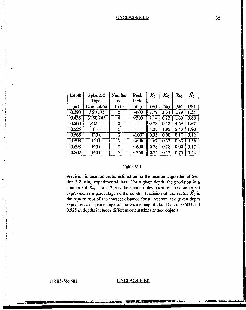
UNCLASSFIED 35

-Dept Spheroid Number Peak X 01 Xo2 Xo 3 XoType, of Field

(m) Orientation Trials (nT) (%) (%) (%) (%)0.390 F90 175 5 ,600 1.79 2.31 1.79 1.35"0.438 M 90 265 4 -300 1.14 0.23 1.60 0.860.500 F,M- - 2 - 0.78 0.12 4.69 1.670.525 F- - 5" 4.27 1.95 5.43 1.900.565 FOO 2 ,-000 0.35 0.00 0.17 0.120.598 FO0 7 -800 1.67 0.33 0.33 0.560.698 F00 2 -600 0.28 0.28 0.00 0.170.802 FO 0 3 ,--,350 0.75 0.12 0.75 0.44

Table VII

Precision in location vector estimation for the location algorithm of Sec-tion 2.2 using experimental data. For a given depth, the precision in acomponent X0o, Z = 1,2, 3 is the standard deviation for the componentexpressed as a percentage of the depth. Precision of the vector X0 isthe square root of the intraset distance for all vectors at a given depthexpressed as a percentage of the vector magnitude. Data at 0.500 and0.525 m depths includes different orientations and/or objects.

DRES-SR-582 UNCLASSIFIEDQ

WIMM M 1M oi

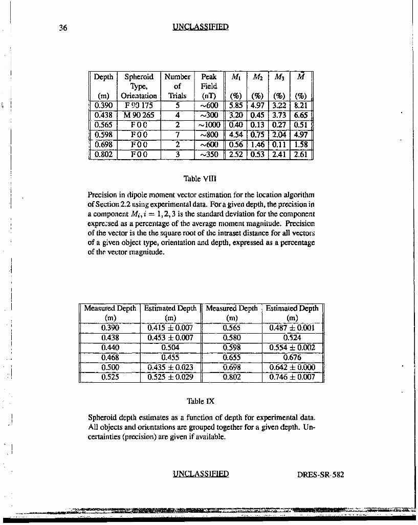
36 UNCLASSIFIED.

Depth Spheroid Number Peak M1 A42 M3 MType, of Field

(m) Orieitation Trials (nT) (%) (%) (%) (%)0.390 F 90 175 5 -,600 5.85 4.97 3.22 8.21

0.438 M90 265 4 ,300 3.20 0.45 3.73 6.650.565 FOO 2 ,-1000 0.40 0.13 0.27 0.510.598 F 00 7 -800 4.54 0.75 2.04 4.97

-0.698 F00 2 -600 0.56 1.46 0.11 1.580.802 FOO 3 ,,,350 2.52 0.53 2.41 2.61

Table VIII

Precision in dipole moment vector estimation for the location algorithmof Section 2.2 using experimental data. For a given depth, the precision ina component Mi, i = 1,2, 3 is the standard deviation for the componentexprezsed as a percentage of the average moment magnitude. Precisionof the vector is the the square root of the intraset distance for all vectorsof a given object type, orientation and depth, expressed as a percentageof the, vector magnitude.

Measured Depth Estimated Depth Measured Depth Estimated Depth(W) (in) W() (W)

0.390 0.415 ±. 0.007 0.565 0.487 + 0.0010.438 0.453 ± 0.007 0.580 0.5240.440 0.504 0.598 0.554 ± 0.0020.468 0.455 0.655 0.6760.500 0.435 ± 0.023 0.698 0.642 ± 0.000

* ! 0.525 0.525 ± 0.029 0.802 0.746 ± 0.007

Table IX

Spheroid depth estimates as a function of depth for experimental data."All objects and orientations are grouped together for a given depth. Un-certainties (precision) are given if available.

UNCLASSIFIED DRES-SR-582

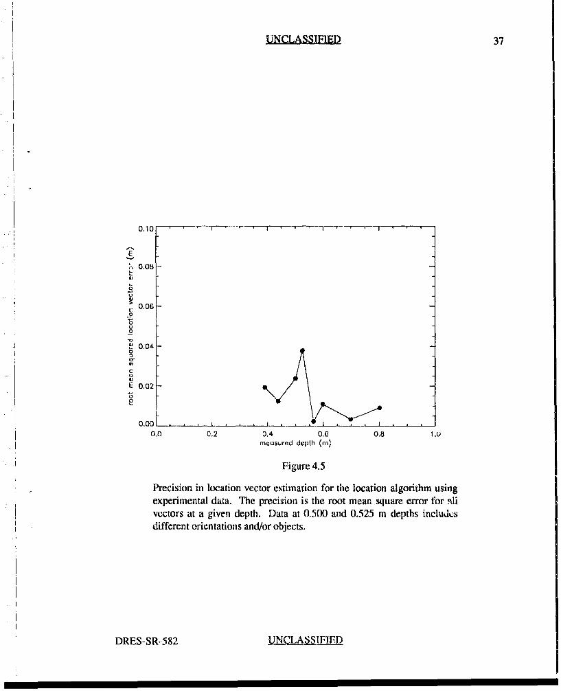
UNCLASSIFIED 37

0.10-----r-- -- r, "'----1-- -''-"'t

IE

00.08

0.06-0

0.06-

.9

0U

E 0. 0a

S0.00

a

E 0.02

0.00 tI . . _.

0.0 0.2 0.4 0.6 0.8 1.umcusured depth (m)

Figure 4.5

Precision in location vector estimation for the location algorithm usingexperimental data. The precision is the root mean square error for .alivectors at a given depth. Data at 0.500 and 0.525 m depths includesdifferent orientations and/or objects.

DRES-SR-.582 LNC1_ASIFIFD

I I I I I II II II II

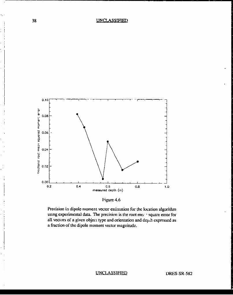
38 UNCLASSIFIED

0.10 ""- - - . -

PI o.08q:

E

S0.06

E O,U4

0.02goa2

0

0.001

0.2 0 4 0.6 0.8 1 .0meosured depth (m)

Figure 4.6

Precision in dipole moment vector estimation for the location algorithmusing experimental data. Tlhe precision is the root mc ' square error forall vectors of a given object type and orientation and deph expressed asa fraction of the dipole moment vector magnitude.

UNCLASSIFIED DRES-SR..582

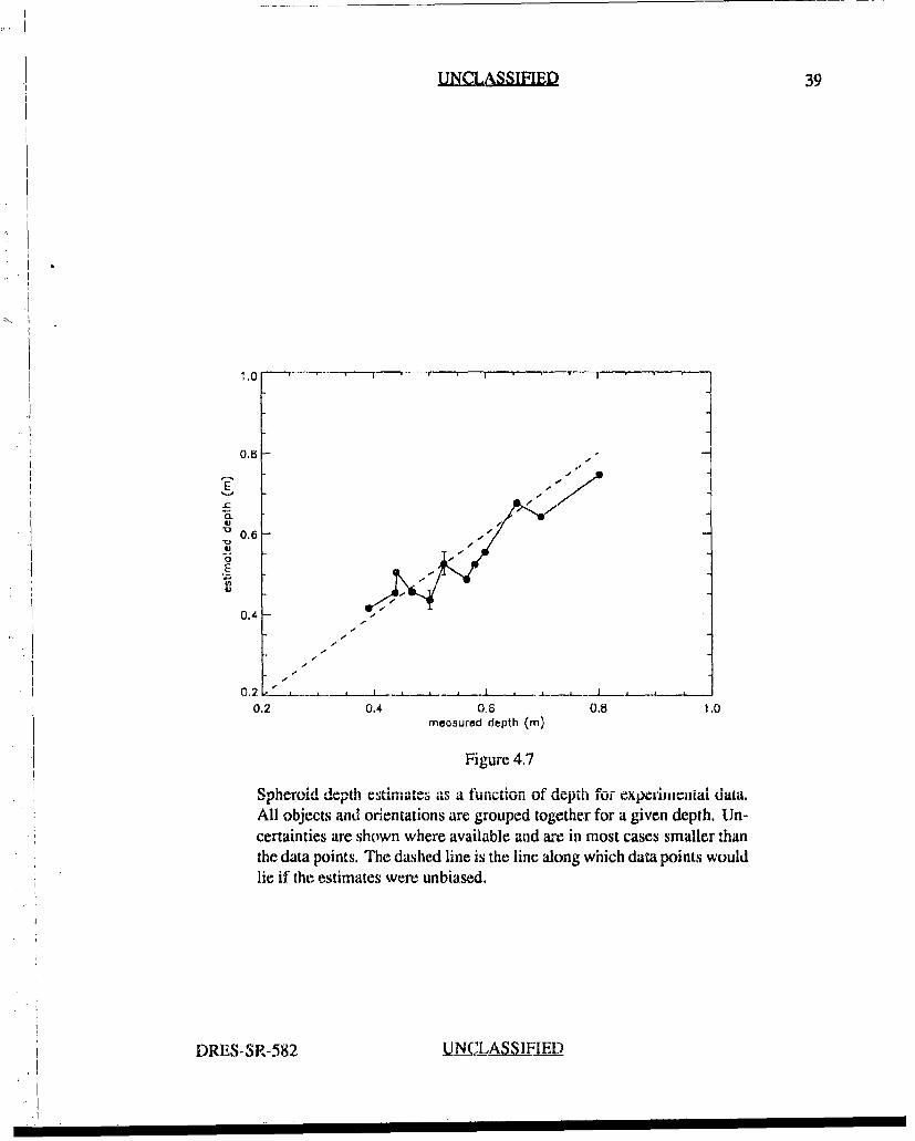
UNLASSIFIED 39

1.0

0.85,

0.65

E

0.40.2

III

-

0.2 4.4 0,6 0.8 1.0

meosured depth (in)

Figure 4.7

Spheroid dIept"h estimates as a *eucino UCpdI'UI x-iIiaa aaiuz~ti u 0 UpUI lutl .,pcIiIlekLa1 data.

All objects and orientations are grouped together for a given depth. Un-certainties are shown where available and are in most cases smaller thanthe data points. The dashed line is the line along which data points wouldlie if the estimates were unbiased.

DRES-SR-582 1N), _LASSIF1ED

40 UNCLASSIFIED

From the data, it can be concluded that there is a depth dependent bias in the estimationof depth. The bias is larger than can be explained by statistical fluctuations. In general,depth estimates are slightly high for small depths and slightly low for large depths. If oneexamines Table V more closely, it can be seen that the algorithm generally underestimatestile depth for 0 < 300 and overestimates for 0 > 60'. An exception is the (90 265)orientation for which one depth is underestimated and two are overestimated. It is alsointeresting to note that the average error in depth is larger for vertical spheroids than itis for higher polar angles (Table V). One explanation is that the negative peak is smallerin magnitude and broader for the vertical case than for larger polar angles, which mightmake the error in estimating the peak position larger. This can be discounted since, if itwere true, the precision in estimates for the vertical spheroid would be worse than for thehorizontal spheroid. However, the precision for the two orientations are similar. A morelikely explanation is that for a given orientation, the octupole field causes the centroids ofthe magnetic field to be shifted from the position of the field extrema. This shift will bea function of the ratio of octupole to dipole field values in the measurement plane, whichwill in turn be dependent on the object orientation. Likewise, the effect of a small amountof remnant magnetization will also be dependent on orientation [7].

'Ib examine the bias in estimation further, it is instructive to look at the bias in estimationof the individual components of the location vector, These are presented in Figures 4.8to 4.10

It is seen that all three components have a depth dependent bias which is larger thancan be accounted for by the precision of the algorithm. The X01 component of the locationis almost always overestimated. The X02 component is generally overestimated for depthsless than 0.55 in and underestimated for depths between 0.55 m and 0.8m. Over the limiteddepth range, the data is consistent with a bias which is periodic with depth, having a 0.25imi period. Further experinments at larger and smaller depths might confirm this, A trendsimilar to that of the X02 component appears to occur for the X03 component except thatthe crossover from overestimation to underestimation occurs at about 0.45 m depth. Thedata may be consistent with a bias which is periodic with depth, but the uncertainties inestimation make determination of the period difficult. Errors in A-3 are generally largerthan those for X01 and X02. 'lThe root mean square (rms) error over all depths is 0.020 mfor X01, 0.019 m for X02 and 0,045 in for X03. This should be compared with the averageprecision for a fixed object and orientation which is 0.005 in for X01, 0.(X)3 m for X02, and0.004 m for X03.

Analysing the bias in the estimation of the dipole moments is more difficult, since the"true" moment components cannot be directly measured as can the location components.We can, however, compare the moment component estimates for a fixed object type andorientation with theoretical values obtained from the model of Section 2.4. Figures 4.11to 4.13 show the variation with depth of the estimates of the three moment componentsfor a type-F spheroid with orientation 0 0. Figures 4.14 to 4.16 show the same thing for atype F spheroid with orientation 90 175 and Figures 4.17 to 4.19 show the variation for atype-M spheroid with orientation 90 265. (Also shown on each Figure are estimates of the

UNl_.,_S1F. D DRES-SR.582

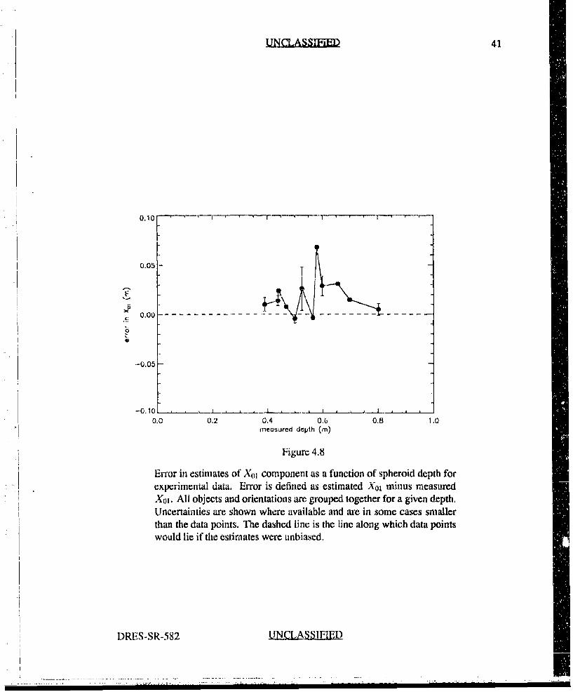
41"

I-1

0.05 --

. 0.00 -

-0.05

-0.1 ,C , . _. • .• .. - .. L. a , •

0.0 0,2 0.4 0,6 0.8 1.0"-'I i~measured depth (m)

Figure 4.8

Error in estimates of X0o component as a function of spheroid depth forexperimental data. Error is defined as estimated X 01 minus measuredX01. All objects and orientations are grouped together for a given depth.Uncertainties are shown where available and are in some cases smallerthan the data points. The dashed line is the line along which data pointswould lie if the estimates were unbiased.

DRES-SR-582 !d.NCLASSIFIED

I

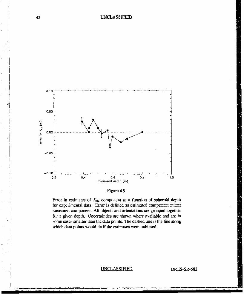
42 UNCLASSIFIED

O,10.''- " I a

0.05

-0.05-

0.2 0.4 0.6 0.8 1.0measured depth (in)

Figure 4.9

Error in estimates of X02 component as a function of spheroid depthfor experimental data. Error is defined nu ...t....d minusmeasured component. All objects and orientations are grouped together

f(,r a given depth. Uncertainties are shown where available and are insome cases smaller than the data points. The dashed line is the line alongwhich data points would lie if the estimates were unbiased.

UNCLASSIFIED DRES-SR-582

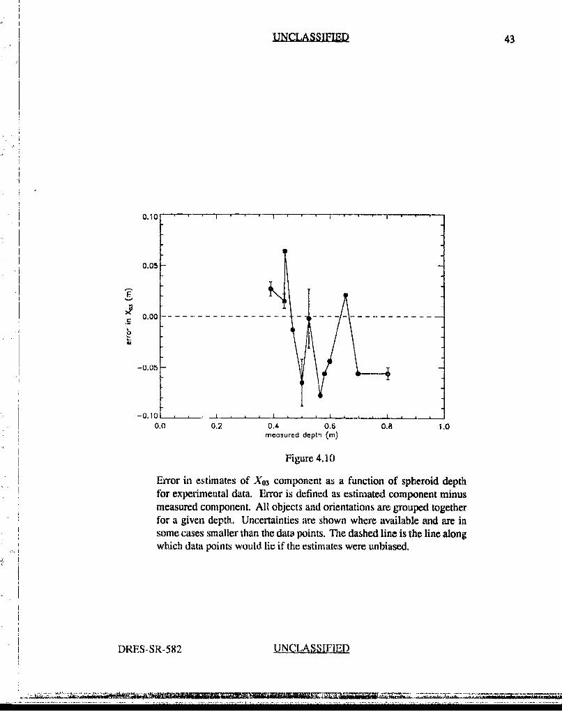
UNCLASSIFIED 43

0. 10o '-• " ,

0.05

F.c• 0 .00 -- -. . - ---.. - -. .- -. .---. .- -. .- -.. ..- -. - -

-0.015

-0.10

0.0 0.2 0.4 0.6 0.8 1.0measured depth (i)

Figure 4. 10

Error in estimates of X 03 component as a function of spheroid depthfor experimental data. Error is defined as estimated component minusmeasured component. All objects and orientations are grouped togetherfor a given depth. Uncertainties are shown where available and are insome cases smaller than the data points. The dashed line is the line alongwhich data points would lie if the estimates were unbiased.

DRES-SR-582 UNCLASSIFIED

44 UNCLASSIFIED

dipole moment components using as input magnetic field maps derived from the model ofSection 2.4. Discussion of these will be deferred to the next Chapter.)

A number of points should be noted about Figures 4.11 to 4.19. There is a deviationbetween theoretical values and experimental estimates that is greater than the uncertainties inthe estimates. Within the confines of the limited number of data points, the deviation does notexhibit a clear trend with depth. To explore a possible trend with object type or orientation,the difference between estimated and theoretical moment components, normalized by themagnitude of the theoretical moment, were plotted for various objects and orientations.For multiple estimates of the same object type and orientation at different depths, theunweighted average of estimates at all depths for that object type and orientation was usedand the uncertainty in estimate was taken to be the standard deviation of the estimates aboutthe average. These results are shown in Figures 4.20 to 4.23.

The unweighted average difference between estimated and theoretical components as apercentage of the theoretical dipole moment is 4.8 ± 7.6% for MI, -3.3 ± 15.5% for M2,-10.8 ± 17.5% for M3 and 24.5 + 11.4% for the root vector difference. There is no cleartrend with object type or orientation. The sources of the estimation bias will be discussedin the next Chapter.

UNCLASSIFIED DRES-SR-582

I I II I II I II I

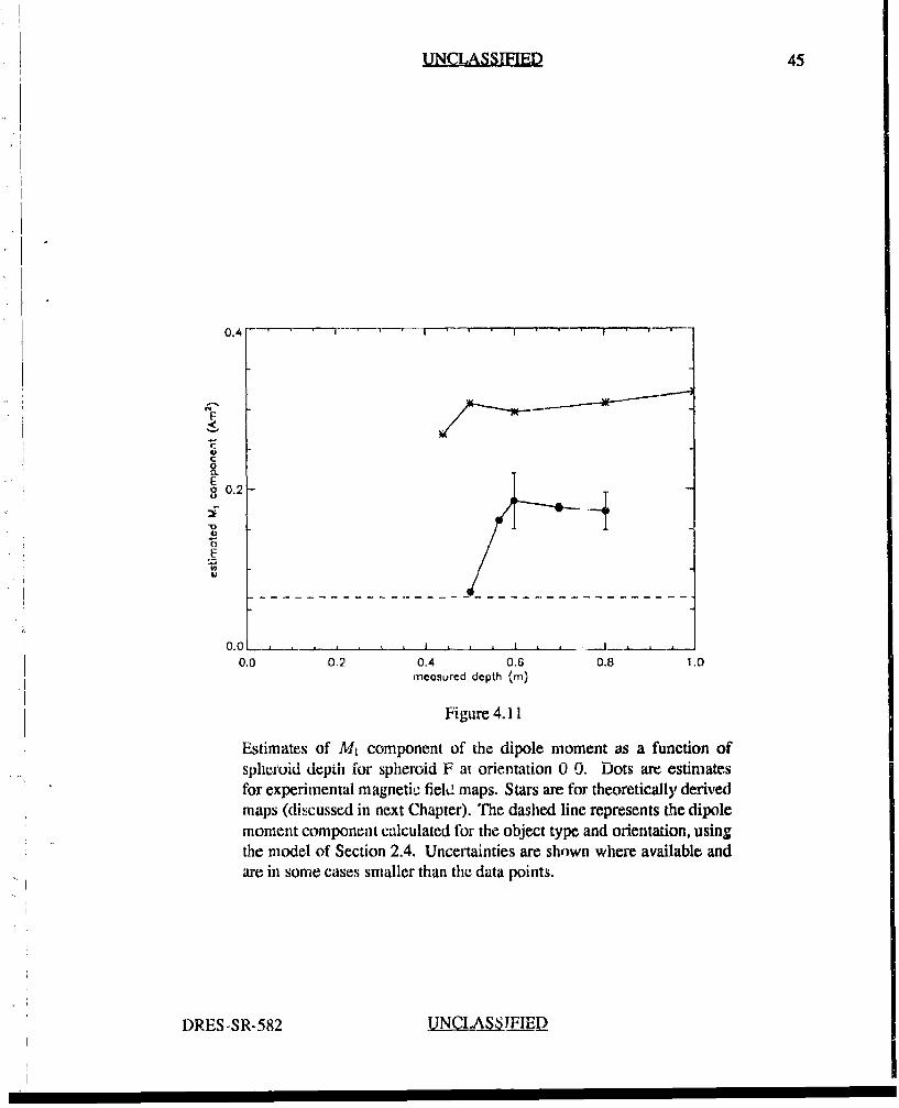
UNCLASSFED 45

0.4 r rI

C

o 0.2 _

,-U

0.0 0.2 0.4 0.6 0.81.0

nmeasured depth I'n)

Figure 4.11

Estimates of M, component of the dipole moment as a function ofsph 'uoid depih for spheroid F at orientation 0 0. Dots are estimatesfor experimental magnetic fiek! maps. Stars are for theoretically derivedmaps (discussed in next Chapter). The dashed line represents the dipolemoment component calculated for the object type and orientation, usingthe model of Section 2.4. Uncertainties are shown where available andare in some cases smaller than the data points.

DRES-SR-582 UNCLASS1LRE

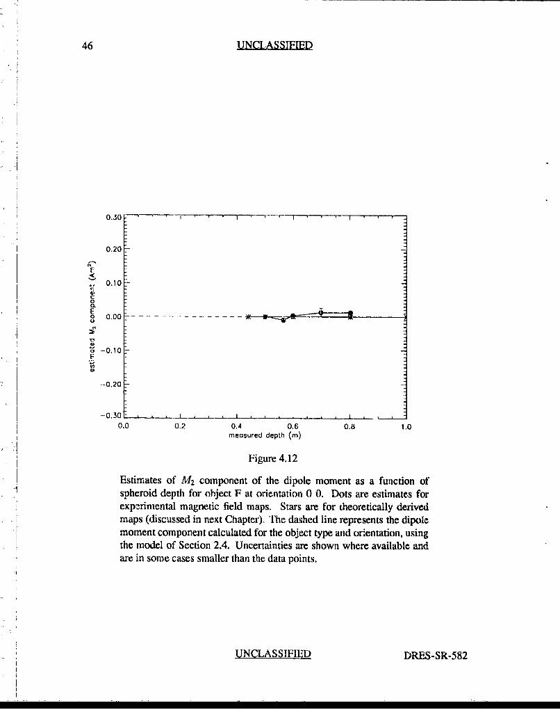
46 UNCLASSIFIED

0.30 --

0.20[

E

0.10C:

0.

0 0.00

o -0.10

--0.20

-0.30 1 , , . _ _ __ __-1 _

0.0 0.2 0.4 0.6 0.8 1.0measured depth (M)

Figure 4.12

Estimates of M2 component of the dipole moment as a function ofspheroid depth for ohject F at orientation 0 0. Dots are estimates forexpzrinmental magnetic field maps. Stars are for theoretically derived

I maps (discussed in next Chapter). The dashed line represents the dipolemoment component calculated for the object type and orientation, usingthe model of Section 2.4. Uncertainties are shown where available andare in some cases smaller than the data points.

IJUNCLASSIFIFD_ DRES-SR-582

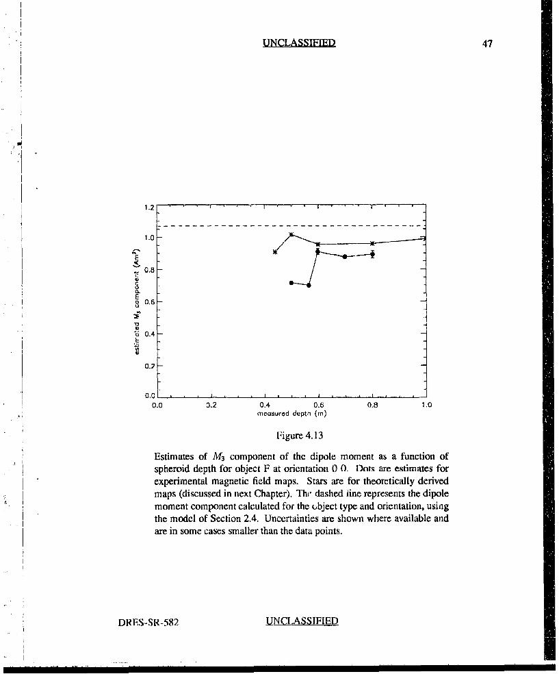
UNCLASSIFIED 47 --

1.2

0.8-

0 0.6

EIUt 0.4

0.2

0.0 0.2 0.4 0.6 0.8 1.0measured depth (mn)

Figure 4.13

Estimates of M3 component of the dipole moment as a function ofspheroid depth for object F at orientation 0 0. Dots are estimates forexperimental magnetic field maps. Stars are for theoretically derivedmaps (discussed in next Chapter). Thr dashed line represents the dipolemoment component calculated for the object type and orientation, usingthe model of Section 2.4. Uncertainties are shown where available andare in some cases smaller than the data points.

DRES-SR-582 -UNCLASSIFIED

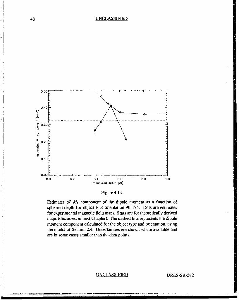
48 UNLASSIFIE

S0,40 [ •

0,30

0)c0.30F

0.10

0.00 - . .I_.

0.0 0.2 0.4 0.6 0.8 1.0measured depth (i)

Figure 4.14

Estimates of M, component of the dipole moment as a function ofspheroid depth for object F at orientation 90 175. Dots are estimatesfor experimental magnetic field maps. Stars are for theoretically derivedmaps (discussed in next Chapter). The dashed line represents the dipolemoment component calculated for the object type and orientation, usingthe modcl of Section 2.4. Uncertainties are shown where available andare in some cases smaller than the. data points.

UNCLASSIFIED DRES-SR-582

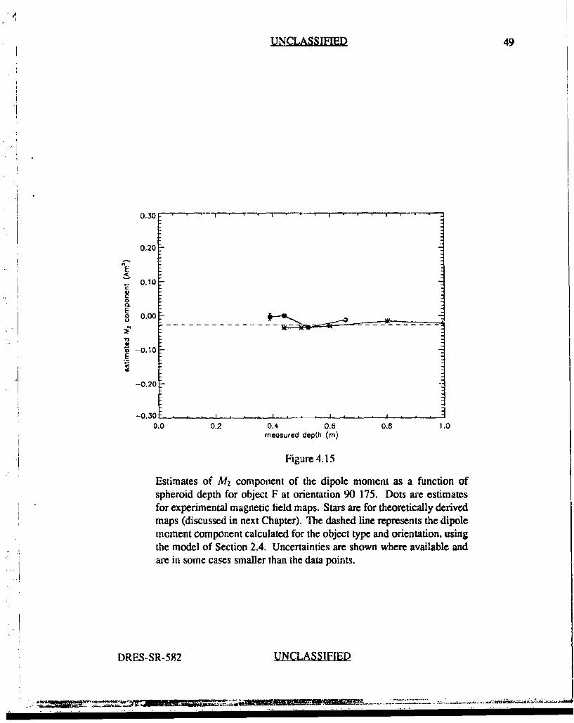
UNCLASSIFIED 49

0.30 ,'-1 ' -,- . -r---T

0.20

E

0.10C4)

0aE0 0.00.-U

"o -o-0-

-0.20

-0.30 . i . . . J . , , I , . , J • , • •

0.0 0.2 0.4 0.6 0.8 1.0meosured depth (m)

Figure 4.15

Estimates of M2 component of the dipole moment as a function ofspheroid depth for object F at orientation 90 175. Dots are estimatesfor experimental magnetic field maps. Stars are for theoretically derivedmaps (discussed in next Chapter). The dashed line represents the dipolemoment component calculated for the object type and orientation, usingthe model of Section 2.4. Uncertainties are shown where available andare in some cases smaller than the data points.

DRES-SR-582 UNCLASSIFIED

I I II i "I . . . I I I I I I I

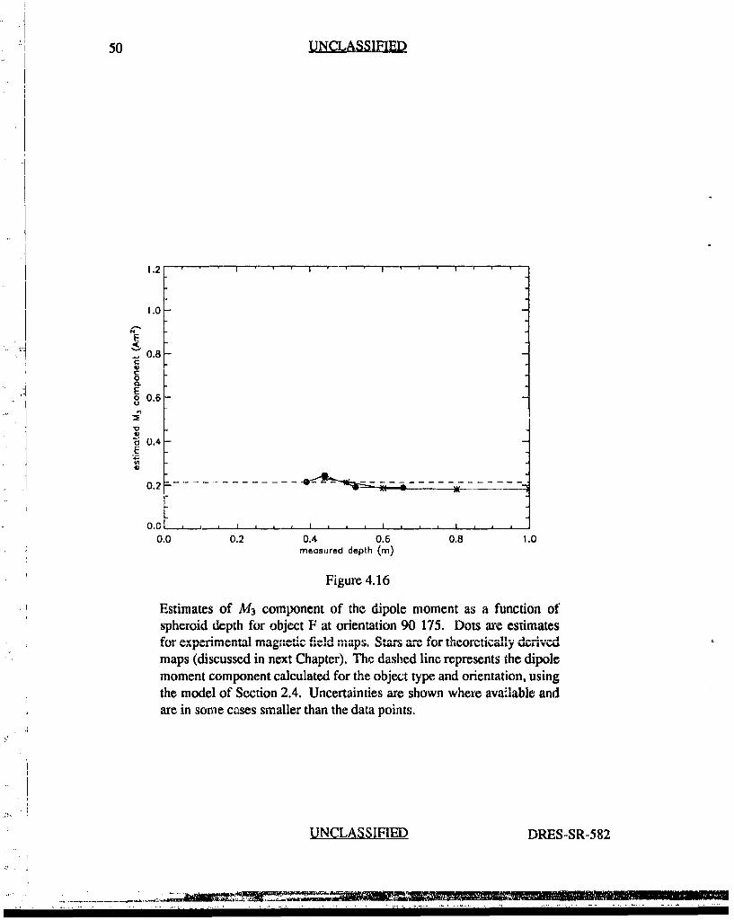
50 UNCLASSIFIED

1 .2

1.0

E

C

0~O

0.4Eo 0.4U'

.10 .2 --- ----------- ---- ------

0.00.0 0.2 0.4 0.6 0.8 1.0

mneasured depth m

Figure 4.16

Estimates of M3 component of the dipole moment as a function ofspheroid depth for object F at orientation 90 175. Dots are estimates

maps (discussed in next Chapter). The dashed line represents the dipolemoment component calculated for the object type and orientation, usingthe model of Section 2.4. Uncertainties are shown where available andare in some cases smaller than the data points.

UNCLASSIFIED DRES-SR-582

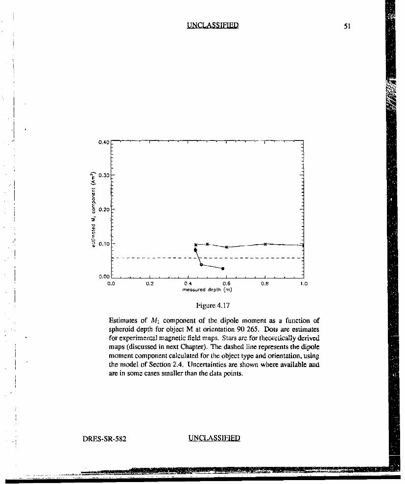
UNCLASSIS 51

"*1 0,40

"F 0.30

E0

0 0.20

'~0.10 -_ _ _ _ _ _ _ _ _---- --- --- --- -) -- -------- - ----- •---

0.00 . _ . I ,

0.0 0.2 0.4 0.6 0.8 1.0meoswred depth (mn)

* IFigure 4.17

Estimates of MI component of the dipole moment as a function ofspheroid depth for object M at orientation 90 265. Dots are estimates

for................ m fi..............,eld p Stars are" theoretually derived

maps (discussed in next Chapter). The dashed line represents the dipolemoment component calculated for the object type and orientation, usingthe model of Section 2.4. Uncertainties are shown where available andare in some cases smaller than the data points.

DRES-SR-582 UN.CLASSIFIED

| I-l- ...-- .- - -

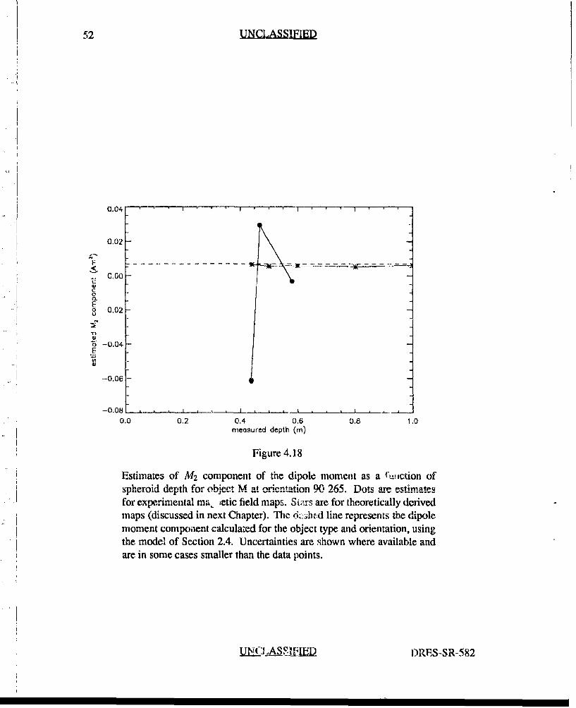
52 UNCLASSIFEDM

0.04 ' I

0.02

-- --- ----------------- ----------- - -- -

0.00--

o -0.02C

-0.04F

--0.06

-~-0.04

0.0 0.2 0.4 0.6 0.8 1.0measured depth (in)

Figure 4.18

Estimates of M2 component of the dipole moment as a fý:iction ofspheroid dept. for ,object. M at orletat, n 0O52)65. Dnts are estimate.for experimental ma, ietic field maps. Si.rs are for theoretically derivedmaps (discussed in next Chapter). The &:cht:d line represents the dipolemoment component calculated for the object type and orientation, usingthe model of Section 2.4. Uncertainties are shown where available andare in some cases smaller than the data points.

U .( LA_ -I..F DRES-SR-582

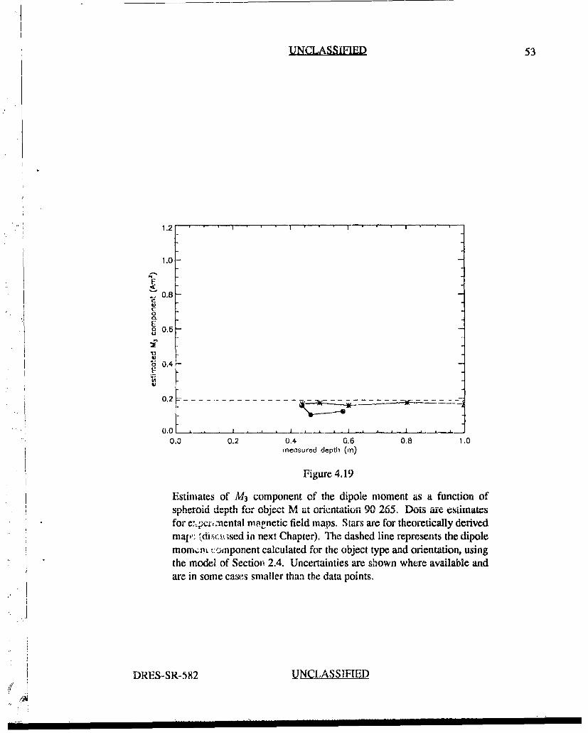
UNCLASSIIED 53

1.0-

~.. 0.84JC

0. oV

0 0.6-U

Wd 0.4

0.0 2_._,__,___J _

0.0 0.2 0.4 0.6 0.8 1.0measured depth (M)

Figure 4.19

Estimates of M3 component of the dipole moment as a function of*, spheroid depth for object M at orientation 9 265. Dots are estiimatesfor ex.pczr-nental magnetic field maps. Stars are for theoretically derivedma.:; fdis..... ,sed in next Chapter). The dashed line represents the dipolemomkn ..:•tnponent calculated for the object type and orientation, usingthe model of Section 2.4. Uncertainties are shown where available andare in some cases smaller than the data points.

DRES-SR-582 UNCLASSIFIED1I

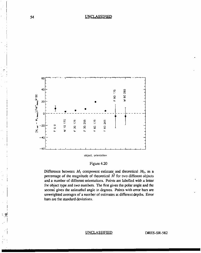
54 UNCLASSIFIED

60 ------------ -r--- Y ' ' "T "

40 L •to

Ch

S20

0.. -6

Ut LfO l I U) --[-4LO to

0-20o o C o 0

-40

--50 . , _L . , I • , I . , . I __ __ _

object, orientation

Figure 4.20

Difference between MI component estimate and theoretical MI, as apercentage of the mgnpitude of theoret-cal M for tw... differn objectS

and a number of different orientations. Points are labelled with a letterfor object type and two numbers. The first gives the polar angle and thesecond gives the azimuthal angle in degrees. Points with error bars areunweighted averages of a number of estimates at different depths. Errorbars are the standard deviations.

-UNCLASSIFIED DRES-SR-582

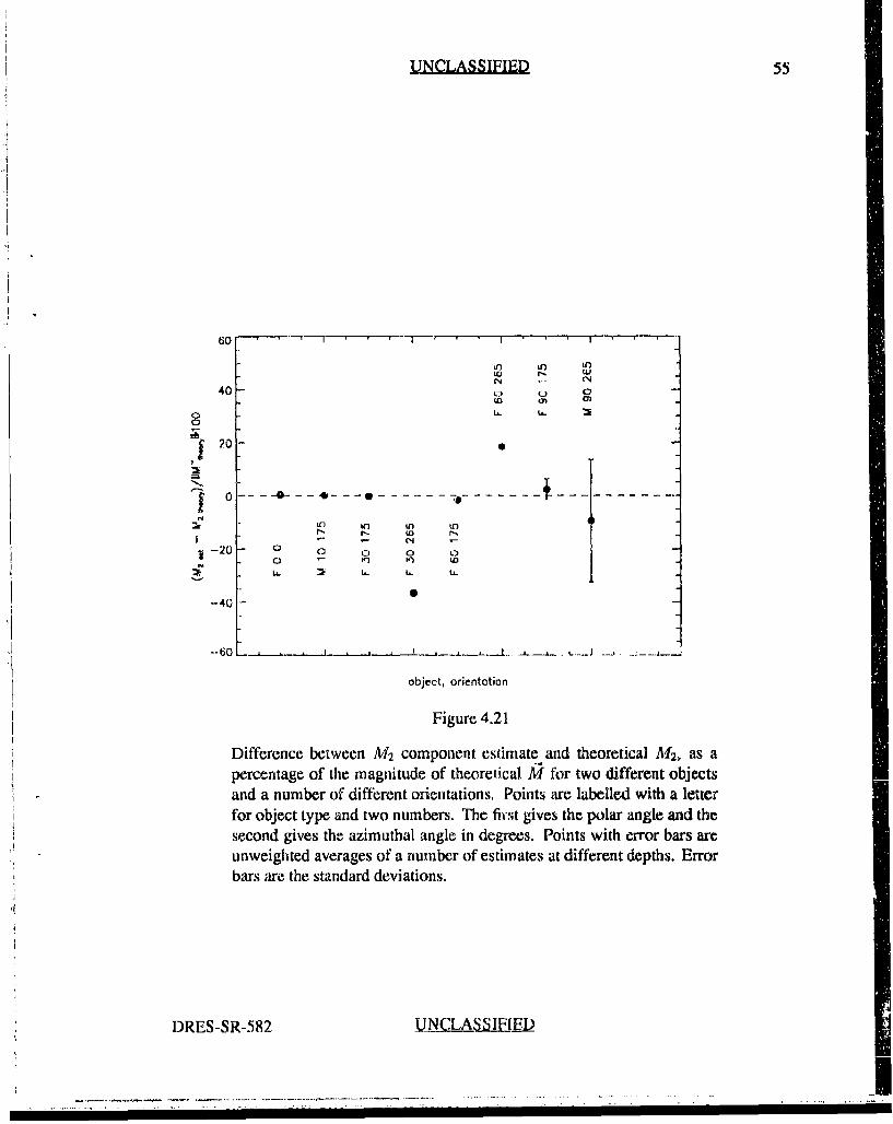
UNCLASSIFIED 55

40 - o 0

20

" 0 -- - - - - - -- - - - -

-to to tn

0 0 o o 00 - ~to ) C

Lt. . :• C. s. is.

-40

--60 ------ s-.---. L__A_- .__ _. .. -L.__ •.._J _, . . .

object, orientation

Figure 4.21

Difference between M2 component estimate and theoretical A12, as apercentage of the magnitude of theoretical Ml for two different objectsand a number of different orientations. Points are labelled with a letterfor object type and two numbers. The fi'st gives the polar angle and thesecond gives the azimuthal angle in degrees. Points with error bars areunweighted averages of a number of estimates at different depths. Errorbars are the standard deviations.

DRES-SR-582 N_.CL U I__ EDI

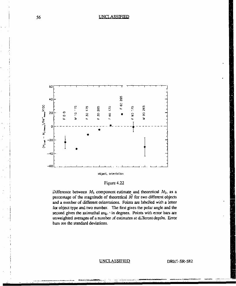
56 UNCLASSIFIED

40 (0

04)2 -I) CI C L• 01

0 PI P • N o

0- - -N - - - - -- --- 00 C) .)

l-20

-40

object, orientation

Figure 4.22

Difference between M3 component estimate and theoretical M3, as a

percentage of the magnitude of theoretical M for two different objectsand a number of different orientations. Points are labelled with a letterfor object type and two number. The first gives the polar angle and thesecond gives the azimuthal ang; - in degrees. Points with error bars are

* unweighted averages of a number of estimates at diLTerent depths. Errorbars are the standard deviations.

N!NLASSIFIED DREU.-SR-582

'Sd........ . .. AZ,•i ..&.t . i- - - - - - n ' " : *d* l* * n~* l **l~

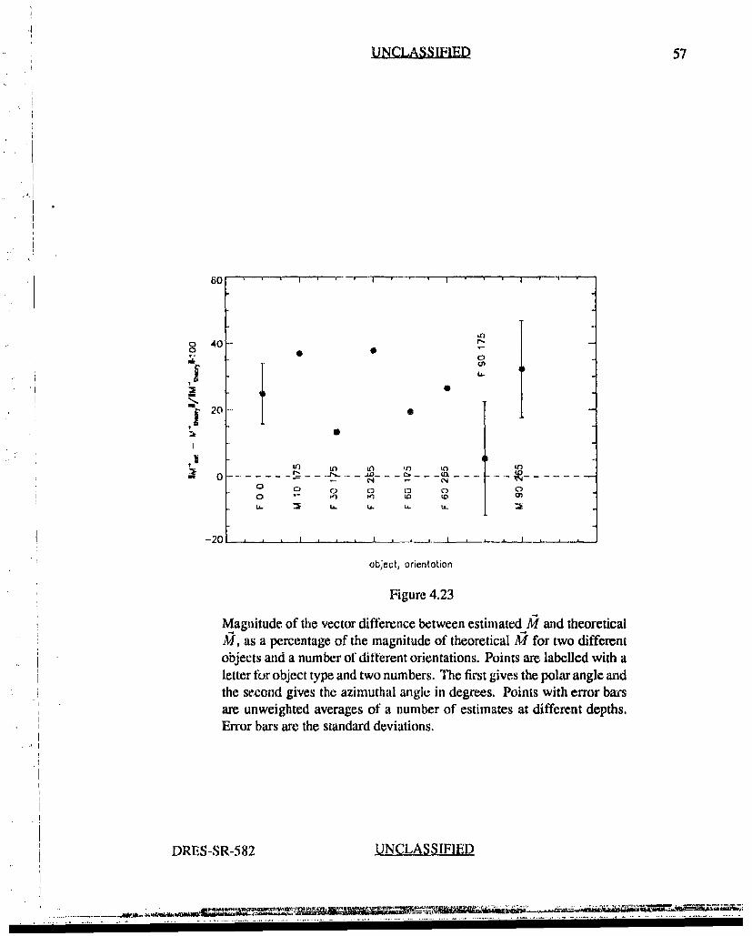
UNCLASSIFIED 57

40 I60

!T1S

o40 r,(

-20 L

t

S• t) L• Ln L01 LO

N -- N4 •0 oD 0 0 3

object, orientation

Figure 4.23

Magnitude of the vector difference between estimated M and theoreticalAM, as a percentage of the magnitude of theoretical M for two differentobjects and a number of different orientations. Points are labelled with aletter fur object type and two numbers. The first gives the polar angle andthe second gives the azimuthal angle in degrees. Points with error barsare unweighted averages of a number of estimates at different depths.Error bars are the standard deviations.

DRES-SR-582 UNCLASSIFIED

S ... •, , • ===• •.• .•_.••" " •:: " •- " . .. •"•• =• • !"ii'

58 UNCLASSIF1EI

UNCLASSIFIED DRES-SR-582

•,,.,.v i~~t~.•at• _ _• ... . _=__1... ... .. . .... . .. ... - - -J.

UNCLASSIIED 59

5. Performance of Location Estimation

5.1 Sources of Error in Location Estimation

In the previous Chapter, we saw that the location algorithm produced estimates of bothlocation and moment components that deviated from the measured or theoretical valuesby amounts that were on average significantly greater than the experimental precision(Figs. 4.20 to 4.23). In this Chapter we will analyse the sources of these deviations in anattempt to identify ways to minimize or eliminate them.

There are a number of possible sources of error in estimating the dipole location andmoment of a compact object when using the algorithm of Section 2.2 with a total fieldmagnetometer. These may be grouped in the following manner:

I. Experimental Errors and Uncertainties

(a) Sensor Positional Uncertainty - Deviations of the sensor from its assumedposition will introduce errors. The dominant error term is due to deviationsof the sensor from a known plane. These have been quantified in [101. Tosummarize briefly, the accuracy of dipole parameter estimates was found to beindependent of twie uncertainty in sensor position parallel to the plane, if thelatter was < 5 % of the depth. The percentage errors in both position and dipolemoment component estimates were roughly equal to the percentage uncertainty(relative to the depth) in sensor position orthogonal to the plane, if the latter was< 5% of the depth.

(b) Finite Volume of Magnetic Sensor Head - The algorithm assumes that a magneticmeasurement is taken at an infinitesimal point in space, but the magnetic sensorhead is a finite cylinder with a length cC 17 cm and a diameter of - 6 cm.The measurement point has been assumed to be the geometric center of theactive volumo.. If the field gradient is small, the measured field will be anaccurate representation of the true field at that point. If the gradient is large,the effective measurement point will be shifted from the geonmetric center byan amount which is a function of the field gradient. This would produce largererrors for objects and orientations whose magnetic field maps have larger fieldgradients. The effect of finite sensor head volume is to introduce a position

DRES-SR-582 UNCLASIFIED

60 I.JNCLASSIFIED

dependent positional uncertainty in all three directions. Properly quantifyingthe uncertainty would require extensive modelling of the operation of the sensorhead in relation to the gradients of the magnetic fields of typical spheroids.

(c) Magnetic Field Measurement Uncertainty - According to [10], assumed zeromean additive Gaussian errors, the accuracy of dipole parameter estimates is in-dependent of SNR of the magnetic field, if the SNR of the field maximum in themeasurement plane is greater than about 25. The smallest maximum encoun-tered in this study was - 100 nT The quantization error for the magnetometersystem is 1 nT, so that the estimates should be independent of SNR. In addition,the spheroid field in the plane can have a large gradient, which combined withpositional uncertainty, will produce errors that are neither Gaussian nor zeromean. Although gradients of ,-, 2 nT/mm for a map with a 1000 nT maximumfield and - 0.3 nT/mm for a map with a 150 nT maximum field were typicallyencountered, these occurred far from the extrema. Gradients near the extremaare, as one would expect, small. (This is, in fact, a strength of the extremumlocation estimator). Thus, errors due to magnetic field measurement uncertaintyare expected to be negligible.

2. Location Algorithm Approximations

(a) Locating the Maximum and Minimum of the Magnetic Field in the MeasurementPlane - A method that was successful with theoretical purely dipolar magneticdata was to search a coarse grid (,-' 25 cm spacing) to quickly approximate themaximum and minimum positions and then to search a fine grid search (,-• 2.5cm spacing) to accurately locate the extrema [10]. For this study, practicalexperimental limitations made it necessary to use only a single search over afixed grid which was fine in the X, di-ection (- 2 - 3 cm spacing) but coarse inthe X2 direction (-, 5 - 10 cm spacing). This may cause an error which is depthdependent, since the spatial extent of the field is a function of depth whereasthe grid spacing is fixed. In addition, the position of the extrerna are located byassuming that the centroid calculated in the vicinity of the extremum coincideswith the extremum position. For skewed peaks, this will produce an error.

(b)" Use ofTotal Magnetic Field Measurmnits - The algorithm, is sturictly speakingcorrect only for vertical component magnetic field measurements. lbtal mag-netic field values approximate, but are not identical to, vertical component valuesin geographical regions with high magnetic inclinations, such as the location ofour laboratory. This will cause a bias in the estimation of dipole parameters, butwill not cause an increase in the standard deviation of the estimates.

(c) errors related to computer implementation. - These include approximations toinverse functions unique to the algorithm and are negligible compared to othersources of error.

3. Deviation of Field of a Compact Object From Pure Induced Dipole

UNCLASSIFIED DRES-SR-582

UNCLASSIFIED 61

(a) Higher Order Moments - Ferrous objects, when placed in a magnetic field,such as that of the earth. acquire induced magnetization whose magnitude anddirection is a function of the primary field strength, ferromagnetic susceptibilityof the body, its shape and its orientation with respect to the primary field.This produces a dipolar field that can be attributed to a dipole moment source

located at the object center. However, for all objects except a sphere, thereare also field components due to higher order moments. These field terms aregenerally smaller than and decrease with distance from the object faster thanthe dipole term. At close distance, the fields due to higher order moments will"add a distortion term to the dipole field and lead to errors in dipole parameterestimation. For the algorithm used in this report, the effect of higher multipolefields is to shift the extrema positions and alter their magnitude. For spheroidssimilar in shape and size to artillery shells at close range in geometries similarto those of these experiments (depth 4 times the maximum dimension and 18times the minimum dimension), the maximum octupole field varies from 3 to8% of the maximum dipole field [81.

(b) Remnant Magnetization -Ferrous objects may also have remnant magnetizationwhich is a function of the metallurgical properties of the object as well as itsthermal, mechanical and geomagnetic history. Remnant magnetization is verydifficult to model since its strength and direction are often unknown for anindividual object and may vary from object to object of the same shape andsize. Remnant magnetization will in general not be purely dipolar. The dipolecomponent of the remnant magnetization will add vectorally to the inducedmoment, which may make it difficult to use the estimated total dipole moment toclassify the object. Higher order multipoles will cause a distortion to the dipolefield, just as those from the induced magnetization do, which will increasethe error in estimating the source location and dipole moment. Fortunately,past evidence has suggested that remnant magnetization can be neglected forsome applications, including ordnance detection 17]. Even when present inartillery shells, some evidence indicates that remnant magnetization is smalland is similar for individual shells of the same type 181.

Of the non-negligible errors mentioned above, positional uncertainties will random innature and will contribute to the precision of the estimates but not the accuracy (bias). Themaximum uncertainties in position were roughly 1.4 cm for X, (determined mainly byth-: finite measurement time of the magnetometer), 1 cm in X2 (dictated by swerving ofthe magnetometer cart) and 0.2 to 0.5 cm in X3 (caused by fluctuations in flatness of themeasurement table). Since the uncertainty in both X, and X2 was < 5% of the depth forall depths, [10] implies that these uncertainties should have a negligible contribution to theoverall precision. Tb compare the measured precision with the precision attributable to thepositional uncertainty, we can average the component precision of the location and momentcomponents of Tables VII and VIII to produce Table X. It is seen that the precision ofestimated location components is in reasonable agreement with 1 101, that is, the average

DRE'S-SR-582 UNCLASSIFIEI)

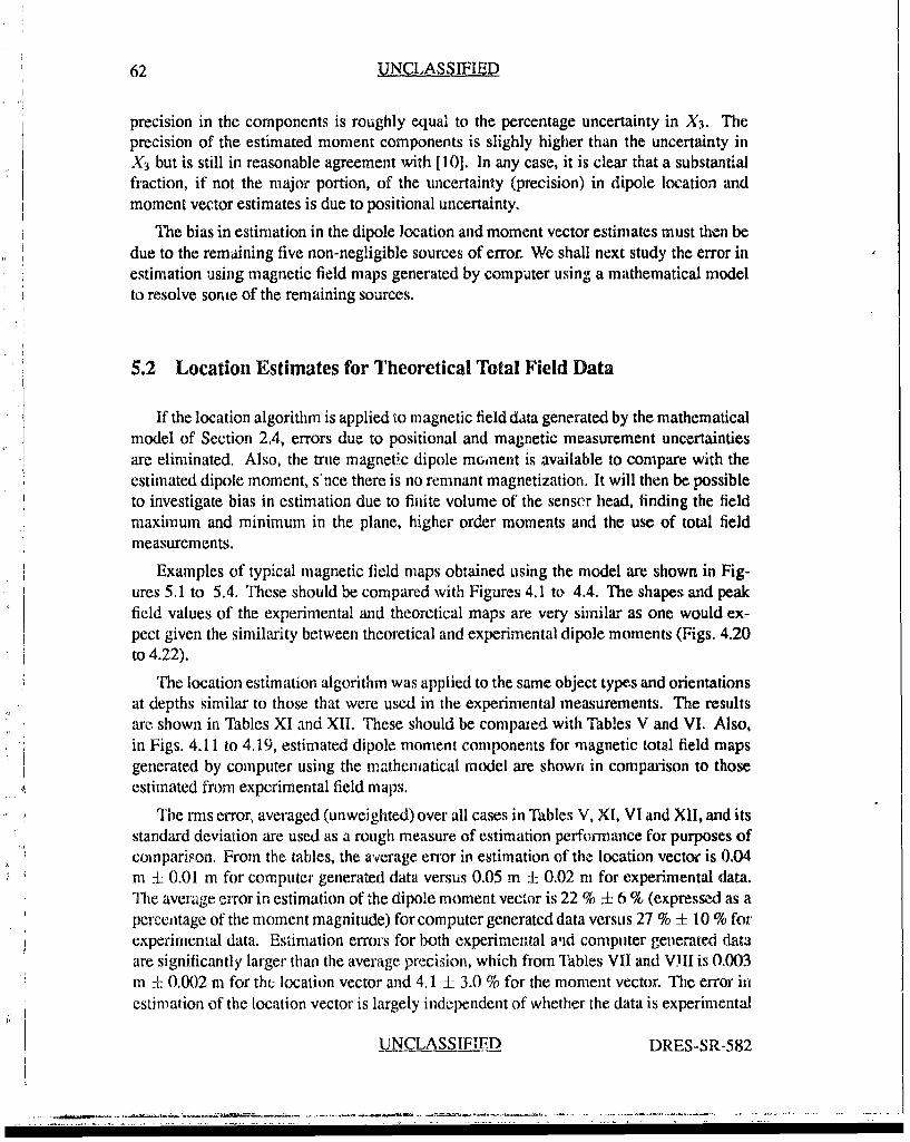
62 U N.LAS SIFIED

precision in the components is roughly equal to the percentage uncertainty in X3 . Theprecision of the estimated moment components is slighly higher than the uncertainty inX3 but is still in reasonable agreement with [10]. In any case, it is clear that a substantialfraction, if not the major portion, of the uncertainty (precision) in dipole location andmoment vector estimates is due to positional uncertainty.

The bias in estimation in the dipole location and moment vector estimates must then bedue to the remaining five non-negligible sources of error. We shall next study the error inestimation using magnetic field maps generated by computer using a mathematical modelto resolve some of the remaining sources.

5.2 Location Estimates for Theoretical Total Field Data

If the location algorithm is applied to magnetic field data generated by the mathematicalmodel of Section 2.4, errors due to positional and magnetic measurement uncertaintiesare eliminated. Also, the true magnetic dipole moment is available to compare with theestimated dipole moment, s'nce there is no remnant magnetization. It will then be possibleto investigate bias in estimation due to finite volume of the sensor head, finding the fieldmaximum and minimum in the plane, higher order moments and the use of total fieldmeasurements.

Examples of typical magnetic field maps obtained using the model are shown in Fig-ures 5.1 to 5.4. These should be compared with Figures 4.1 to 4.4. The shapes and peakfield values of the experimental and theoretical maps are very similar as one would ex-pect given the similarity between theoretical and experimental dipole moments (Figs. 4.20to 4.22).

The location estimation algorithm was applied to the same object types and orientationsat depths similar to those that were used in the experimental measurements. The resultsare shown in Tables XI and XII. These should be compaxed with Tables V and VI. Also,in Figs. 4.11 to 4.19, estimated dipole moment components for magnetic total field mapsgenerated by computer using the mathematical model are shown in comparison to thoseestimated from experimental field maps.

The rms error, averaged (unweighted) over all cases in Tables V, XI, VI and XII, and itsstandard deviation are used as a rough measure of estimation performance for purposes of

* comparison. From the tables, the average error in estimation of the location vector is 0.04m ± 0.01 m for computer generated data versus 0.05 m ± 0.02 m for experimental data.The average error in estimation of the dipole moment vector is 22 % ± 6 % (expressed as apercentage of the moment magnitude) for computer generated data versus 27 % ± 10 % forexperimental data. Estimation errors for both experimental a'nd computer generated dataare significantly larger than the average precision, which from Thbles VII and VIII is 0.003m ± 0.002 m for thu location vector and 4.1 ± 3.0 % for the moment vector. The error inestimation of the location vector is largely independent of whether the data is experimental

UNCLASSIFIED DRES-SR-582

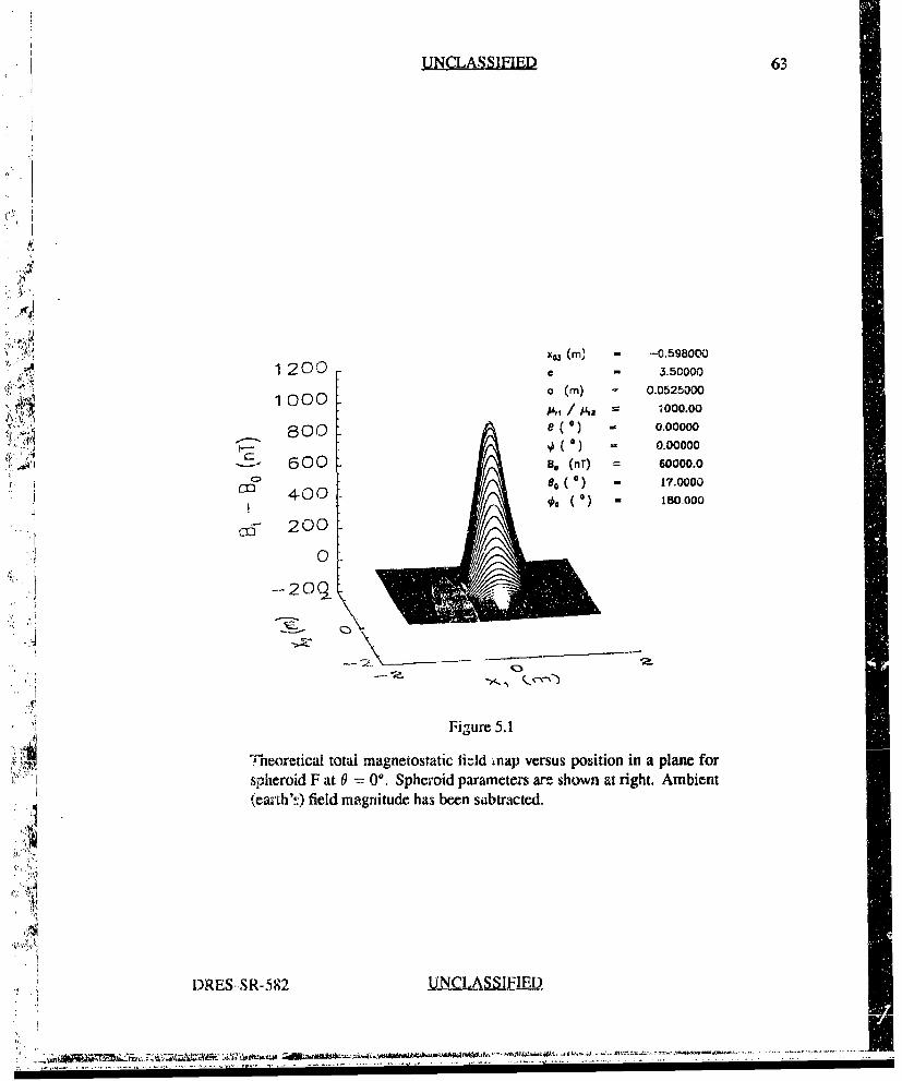
UNCLASSIED 63

" " (M

"�•• (in) ,, -0.598000

1200 e - 3.500001000 o (mi) 0.0525000

1000," 1000.00

80 00) - 0.0000080 0.00000

.,-- 600 B. (nT) 60000,00 17.0000

cn 400 *o (0) = 180.000

rn 200

0

-- 09

Figure 5.1

s neoretical totai magnetostatic field inap versus position in a plane for

spheroid F at 0 = 0°. Spheroid parameters are shown at right. Ambient

(earth's) field magnitude has been subtracted.

DRES -SR-52 UNC_ .A -I EIE D.

• .. tl:U .t1h~t~ XM~ ~ . N- . -

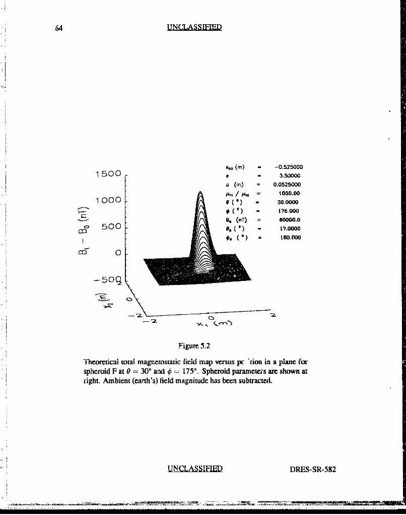
64 UNCLASI, IE12

X03 (M) - -0.5250001500 e 3.50000

a (in) = 0.0525000/4, / /•2 = 1000.00

1000 0(°) - 30.0Mo

*(O) 1?7.000

Bo (nT) = 60000.0

500 0(0) - 17.0000

0C0M'0 9 ,) . 180.000CI 0

-509

2 -.

Figure 5.2

Theoreticai totai magncmostatic field map versus pc "[ion in a piane forspheroid F at 0 = 300 and 4' 1750. Spheroid parameters are shown atright. Ambient (earth's) field magnitud has been subtracted.

UNLASSIFED DRES-SR-582

UNCLASSIFIED 65

1000 • (iln - -(M2)1000 3.50000

o (m) = 0.0525000800/ ,Oo.•o

) - 80.0000-,, "'" 600 17•.o00

--- . (nT) 86000.0. 400 - 17.0000co3 go (0)

*' 200 * (') - 180.000

* 0

-20g

Figure 5.3

Theoretical total magnetostatic field map versus position in a plane forspheroid F at 0 =, 60* and qb = 175°.Spheroid parameters are shown atright. Ambient (earth's) field magnitude has been subtracted.

DRE-S-SR-582 U.NCLA$SIE!I,

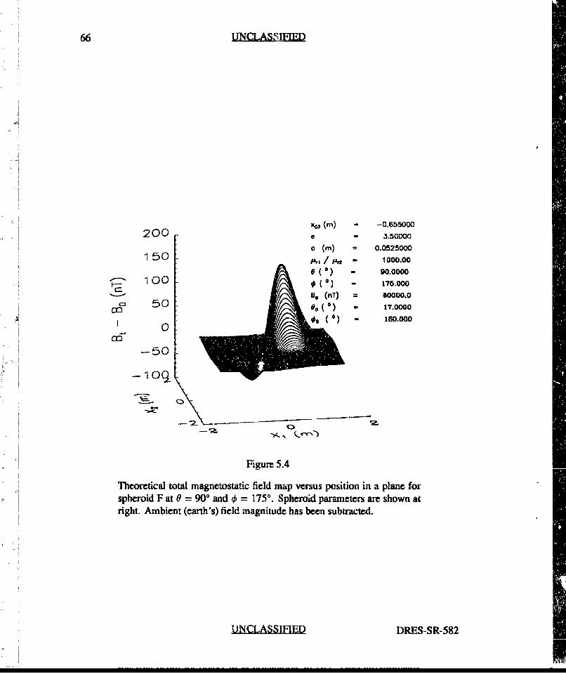
66 UNCLASEIEID

xO, (m) = -0.655000200 : - 3.soooo

S(in) -- 0.0525000

150 /,Ar / f 1000.00

e 90.0000• • 100 t 175.000

0-, (nT) = 60000.050, 0( 17.0000

*0 • (o) - iao.ooo0.

-50

Figure 5.4

Theoretical total magnetostatic field map versus position in a plane for

spheroid F at 0 = 90' and 0 = 1750. Spheroid parameters are shown atright. Ambient (earth's) field magnitude has been subtracted.

UNCLASSWMIF D DRES-SR-582

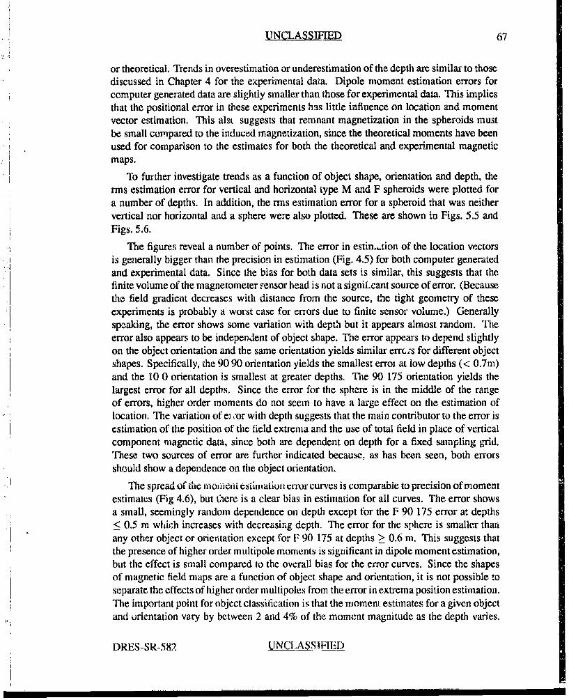
UNCLASSIUFID 67

or theoretical. Trends in overestimation or underestimation of the depth are similar to thosediscussed in Chapter 4 for the experimental data. Dipole moment estimation errors forcomputer generated data are slightly smaller than those for experimental data. This impliesthat the positional error in these experiments has little influence on location and momentvector estimation. This alst suggests that remnant magnetization in the spheroids mustbe small compared to the induced magnetization, since the theoretical moments have beenused for comparison to the estimates for both the theoretical and experimental magneticmaps.

To further investigate trends as a function of object shape, orientation and depth, therms estimation error for vertical and horizontal type M and F spheroids were plotted fora number of depths. In addition, the rms estimation error for a spheroid that was neithervertical nor horizontal and a sphere were also plotted. These are shown in Figs. 5.5 andFigs. 5.6.

The figures reveal a number of points. The error in estin.,.tion of the location vectorsis generally bigger than the precision in estimation (Fig. 4.5) for both computer generatedand experimental data. Since the bias for both data sets is similar, this suggests that thefinite volume of the magnetometer sensor head is not a signii-cant source of error. (Becausethe field gradient decreases with distance from the source, the tight geometry of theseexperiments is probably a worst case for errors due to finite sensor volume.) Generallyspeaking, the error shows some variation with depth but it appears almost random. llieerror also appears to be independent of object shape. The error appears to depend slightlyon the object orientation and the same orientation yields similar errc:s for different objectshapes. Specifically, the 90 90 orientation yields the smallest erroi at low depths (< 0.7m)and the 10 0 orientation is smallest at greater depths. The 90 175 orientation yields thelargest error for all depths. Since the error for the sphere is in the middle of the rangeof errors, higher order moments do not seemn to have a large effect on the estimation oflocation. The variation of ei ,or with depth suggests that the main contributor to the error isestimation of the position of the field extrema and the use of total field in place of verticalcomponent magnetic data, since both are dependent on depth for a fixed sampling grid.These two sources of error are further indicated because, as has been seen, both errorsshould show a dependence on the object orientation.

T hle spread of the InoineW estination error curves is comparable to precision of momentestimates (Fig 4.6), but there is a clear bias in estimation for all curves. The error showsa small, seemingly random dependence on depth except for the F 90 175 error at depths< 0.5 m which increases with decreasing depth. The error for the sphere is smaller thanany other object or orientation except for F 90 175 at depths > 0.6 m. This suggests thatthe presence of higher order multipole moments is significant in dipole moment estimation,but the effect is small compared to the overall bias for the error curves. Since the shapesof magnetic field maps are a function of object shape and orientation, it is not possible toseparate the effects of higher order multipoles from the error in extrema position estimation.The important point for object classification is that the moment: estimates for a given objectand urientation vary by between 2 and 4% of the moment magnitude as the depth varies.

DRES-SR-582 .NQ AS IFIED

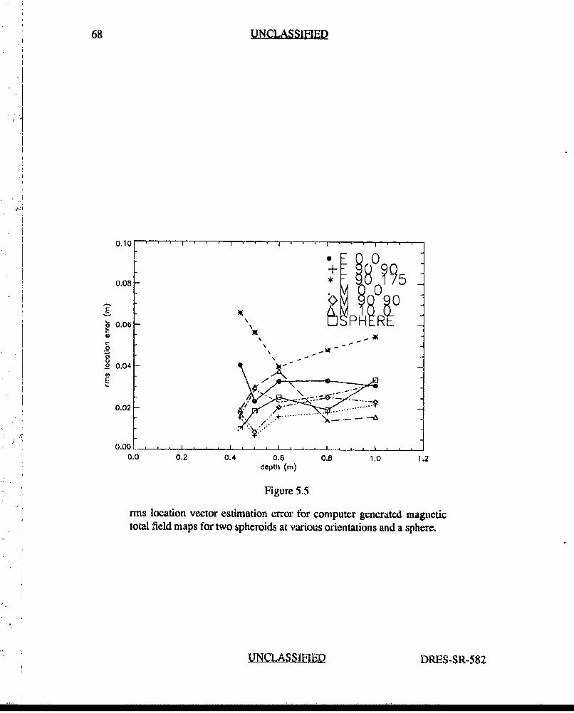
68 UNCLASSIFIED

0. 10 l- --- T-I1'I '

I+

A 0?0

S 0.04-S

ic

U'"t0.04

0.00 -

0.0 .L .I . ' PHERE.L ~ L~.

0.0 0.2 0.4 0.6 0.8 1.0 1.2depth (M)

Figure 5.5

rms location vector estimation error for computer generated magnetictotal field maps for two spheroids at various orentations and a sphere.

• UNCLASS•IFIED DRES-SR-582

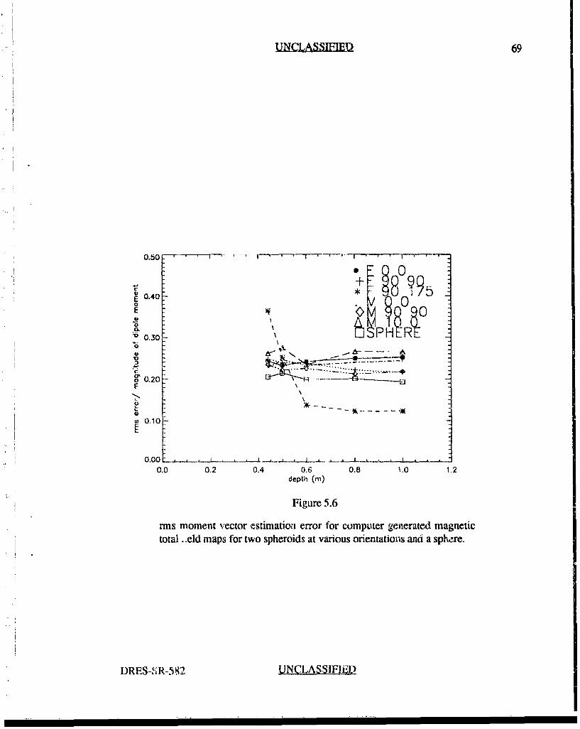
UNCLASSIIED 69

0.i

I+

O.bhO - - I -- ''.•- i I • ' -

E 0.40

"0 0.30 PH\

E w

Fo.0.20--

S0.10

0.00 .4J-0.0 0.2 0.4 0.6 0.8 1.0 1.2

depth (m)

Figure 5.6

rms moment vector estimation error for computer generated magnetictotal .eld maps for two spheroids at various orientations and a sphere.

DRES-SR-5 92 UNCLASSIF1EIED

70 UNCLASSIFIED

The bias is unimportant, since the estimated moments can be used in the design set. Thissuggests that the limiting misclassification error will be between roughly 1.4 and 2.4% [11]if the experimental error is substantially less than the algorithmic and approximation errors.For the present experimental precision (4.1 ± 3.0% ), the misclassification error should beroughly between 2 and 5% (assuming quadrature error summation) if the design set wereexperimentally obtained.

For both the location and dipole moment estimation the F 90 175 curves do not followthe same trends as the others. The location enor is higher tb.An the other errors while themoment curve has a sharp depth dependency not seen in the other moment errors. Thereason for this is not known.

It is initially tempting to think that one can estimate the remnant dipole moment bysubtracting the dipole moments estimated for experimental maps from those estimatedfor theoretical maps with object type, orientation and depth fixed (Figs. 4.11 to 4.19).Averaging over depth would then give the remnant magnetization for a given object andorientation (which should be related to other orientations by a simple Euler rotation matrix).Unfortunately, as we have just seen, the bias in estimation varies with object orientation.This is presumably due to the differing shapes of the magnetic maps which have differenterrors when estimating the extrema positions. This variation is small but is clearly of thesame order of magnitude as the deviation between experimental and theoretical estimates.A simple subtraction of experimental and theoretical moment estimates would not takeinto account the difference in bias due to the differing moments of the experimental andtheoretical data. There may be ways to more precisely estimate the contribution of remnantmagnetization to the total dipole moment. For example, one might use theoretical momentsto derive the error bias as a function of moment component estimates. 'Phis could, in turn,"be applied a, a correction to the expurimental estimates. Then, one could subtract thetheoretical dipole moments from the corrected experimental estimates. It is hoped that thiscan be investigated in the future.

5.3 Location Estimates for Theoretical Vertical Component Field Data

From the previous section, it was seen that, if we exclude experimental errors (positional

uncertainty and remnant magnetization), there are three other possible sources of error thatcan contribute significantly to the estimation error. T'1 se are the estimation of extremapositions, the use of total field magnetic data and the presence of higher order moments.To eliminate the effect of using the total magnetic field of the spheroid as an approximationto the vertical component of the magnetic field, the location algorithm was applied tomragnelic field maps of the vertical magnetic component (B.3). The rms estimation errt.was calculated for the same objects, orientations and depths as in Figs. 5.5 and 5.6. Theseare shown in Figs. 5.7 and Figs. 5.8.

The error in estimation of the location vector is generally slightiy smaller for a givencase than when total field data are used. Other trenis are vry .;imilar to the total field data.

I jJNLAII[ŽL-t) DRES--SR-582

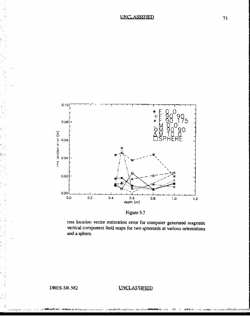
UNCLASSIFIED 71

o0004 ..

0.02- PH R -

2'

-9 004 : ),K-•,

0.0 0.2 0.4 0.6 0.8 1.0 1.2depth (i)

Figure 5.7

rms location vector estimation error for computer generated magneticvertical component field maps for two spheroids at various orientationsand a sphere.

DRES-SR-582 NIASSFIED

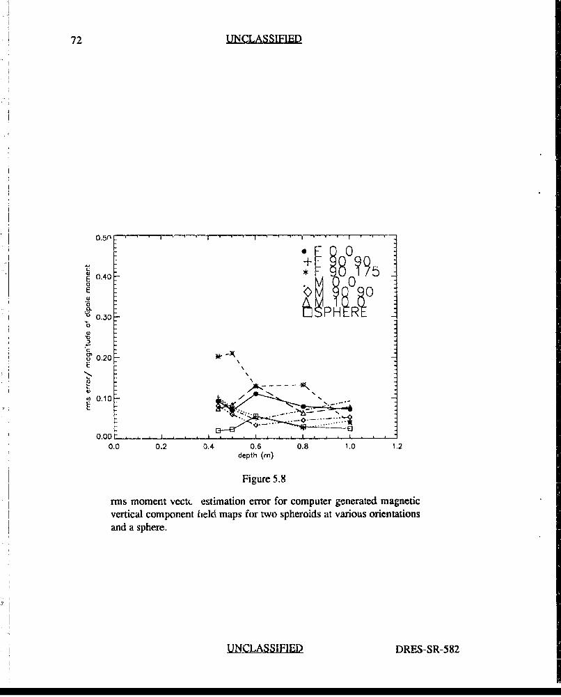
72 UNCLASSIFIED

0.40l

E0.0 0

aa0.30 R

a0.20 AtE

p0.10

0,00 , I I . . . .. .

0.0 0.2 0.4 0.6 0.8 1.0 1.2depth (in)

Figure 5.8

rms moment vecti- estimation error for computer generated magneticvertical component field maps for two spheroids at various orientationsand a sphere.

UINJCILA DRES-SR-582

UNCLASSIFIED 73

Again the depth dependency is small and almost random in nature. The error for the sphereis, as before, not the lowest for all cases. The 90 175 case again yields the highest error atall depths, except for M 90 90 at 0.5 in. It is not clear why the error for this latter case isanomalously high.

The spread in moment est'mation error for vertical component data is similar to that ofthe total field data, but the bias for the former is significantly less. This suggests that theuse of total field data introduces a bias in estimation for - dipole moment. As for the totalfield data, the error for vertical component data is roughly constant with depth for a givenobject and orientation. The error in estimation of the sphere is significantly less than allother cases except M 90 90 and M 0 0 at 0.6 m depth, which indictates that higher ordermoments still contribute somewhat to the error. To crudely estimate the contribution ofthe various sources of error, we note that the bias in estimation of the sphere for verticalcomponent data is roughly 2 to 6% of the moment magnitude, whereas for total field datait is 20%. This suggests that the error due to the total field approximation varies from14 to 18% of the moment magnitude. Error due to estimation of extrema positions andhigher order moments then varies from 0 to 8% of the moment magnitude which is in roughagreement with that for the total field data. This seems reasonable, since in Section 5.1 itwas noted the maximum octupole field varies from 3 to 8% of the maximum dipole fieldfor spheroids in geometries similar to ours.

DRES-SR-582 UN LASSIFIED

I I I I I NOIW

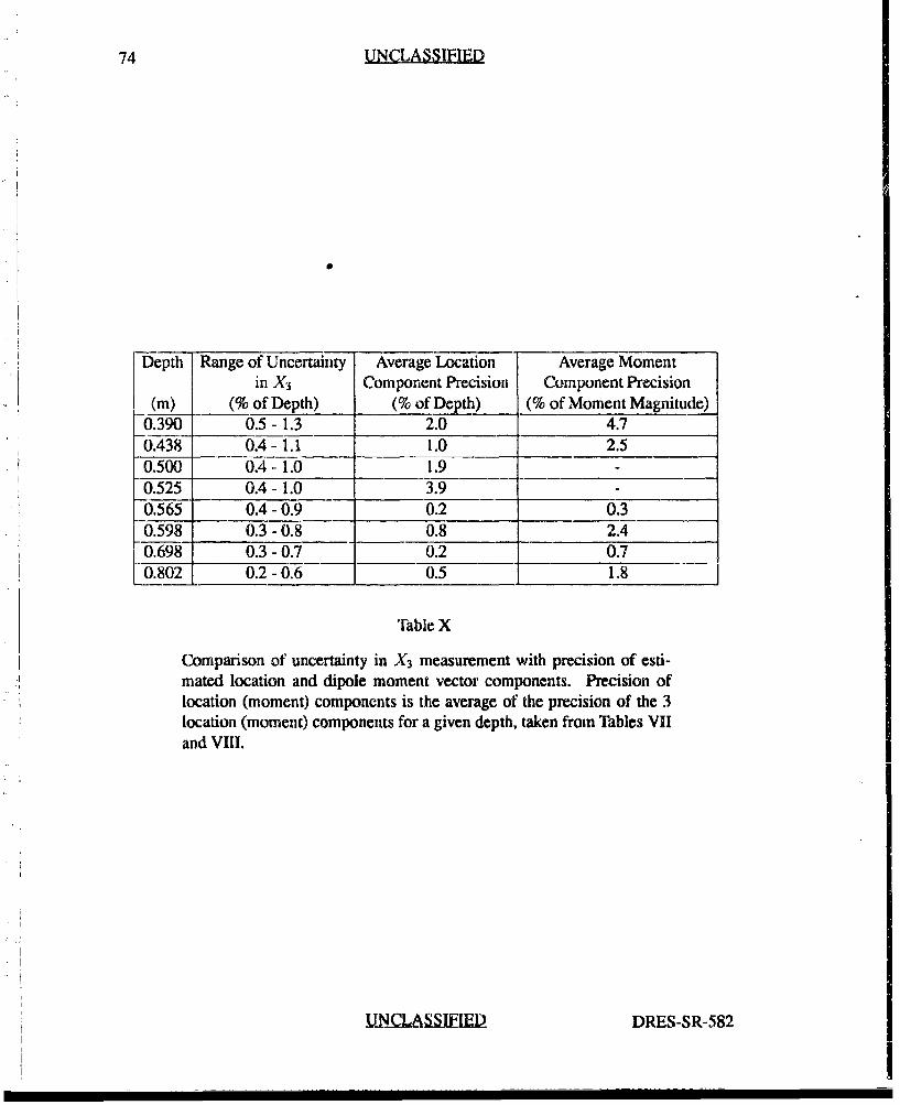
74 UNCLASSIFIED

Depth Range of Uncertainty Average Location Average Momentin X3 Component Precision Component Precision

(W) (% of Depth) (% of Depth) (% of Moment Magnitude)0.390 0.5- 1.3 2.0 4.70.438 0.4- 1.1 1.0 2.50.500 0.4- 1.0 1.9 -0.525 0.4- 1.0 3.9 -0.565 0.4 - 0.9 0.2 0.30.598 0.3 - 0.8 0.8 2.40.698 0.3 - 0.7 0.2 0.70.802 0.2-0.6 0.5 1.8

"fable X

Comparison of uncertainty in X3 measurement with precision of esti-mated location and dipole moment vector components. Precision oflocation (moment) components is the average of the precision of the 3location (moment) components for a given depth, taken from Tables VIIand VIII.

LN._LS SIFIED DRES-SR-582

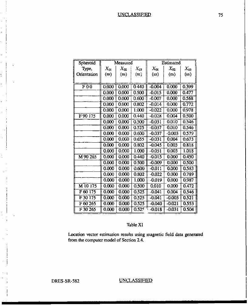
UNCLASSIFIED 75

Spheroid Measured Estimated

Ty3pe, X01 X02 X03 Xo, Xo2 X03Orientation (m) (m) (m) (in) (m) (m)

F 00 0.000 0.000 0440 -0.004 0.000 0.3990.000 0.000 0.500 -0.015 0.000 0.4770.000 0.000 0.600 -0.007 0.000 0.568

.0.000 0.000 0.802 -0.014 0.000 0.7720.000 0.000 1.000 -0.022 0.000 0.978

F 90 175 0.000 0.000 0.440 -0.028 0.004 0.5000.000 0.000 0.500 -0.031 0.010 0.5460.000 0.000 0.525 -0.037 0.010 0.5460.000 0.000 0.600 -0.037 -0.003 0.579

10.000 0.000 0.655 -0.031 0.004 0.673_0.000 0.000 0.802 -0.045 0.003 0.818

0.000 0.000 1.000 -0.051 0.003 1.018M 90 265 0.000 0.000 0.440 -0.015 0.000 0.450

0.000 0.000 0.500 -0.009 0.000 0.5000.000 0.000 0.600 -0.011 0.000 0.5830.000 0.000 0.802 -0.022 0.000 0.7890.000 0.000 1.000 -0.019 0.000 0.987

M 10 175 0.000 0.000 0.500 0.010 0.000 0.472F 60 175 0.000 0.000 0.525 -0.041 0.004 0.546F 30 175 0.000 0.000 0.525 -0.041 -0.003 0.521F 60 265 0.000 0.000. 0.525 -0.040 -0.021 0.553F 30265 0.00020.000 0.525 ';-0.018 -0.031 ,0.5041

Table XI

Location vector estimation results using magnetic field data generatedfrom the computer model of Section 2.4.

DRES-SR-582 UNC.LLASSIFIED

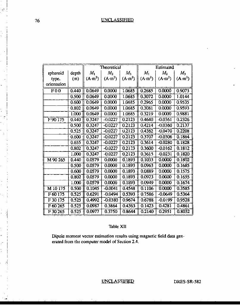
76 UNCLASSIFIED

oniTheoretical Estimatedspheroid depth MA M2 Ar M, M12 M3

type, (in) (A m2) (A.m 2) (A.m 2) (A.m 2) (A.m 2 ) (A.m2)orientation 1

F00 0.440 0.0649 0.0000 1.0685 0.2685 0.0000 0.90730.500 0.0649 0.0000 1.0685 0.3072 0.0000 1.01440.600 0.0649 0.0000 1.0685 0.2965 0.0000 0.95350.802 0.0649 0.0000 1.0685 0.3081 0.0000 0.95931.000 0.0649 0.0000 1,0685 0.3219 0.0000 0.9881

F 90 175 0.440 0.3247 -0.0227 0.2123 0.4640 -0.0361 0.23260.500 0.3247 -0.0227 0.2123 0.4214 -0.0360 0.21370.525 0.3247 -0.0227 0.2123 0.4362 -0.0470 0.22080.600 0.3247 -0.0227 0.2123 0.3707 -0.0306 0.18640.655 0.3247 -0.0227 0.2123 0.3614 -0.0280 0.18280.802 0.3247 -0.0227 0.2123 0.3600 -0.0162 0.18121.000 0.3247 -0.0227 0.2123 0.3615 -0.0231 0.1820

M 90 265 0.440 0.0579 0.0000 0.1893 0.1033 0.0000 0.18020.500 0.0579 0.0000 0.1893 0.0963 0.0000 0.16850.600 0.0579 0.0000 0.1893 0.0889 0.0000 0.15750.802 0.0579 0.0000 0.1893 0.0923 0.0000 0.16551.000 0.0579 0.0000 0.1893 0.0949 0.0000 0.1674

M 10 175 0.500 0.1045 -0.0041 0.4548 0.1106 0.0000 0.3585F 60 175 0.525 0.6291 -0.0494 0.5393 0.7586 -0.0649 0.5364F 30 175 0.525 0.4992 -0.0380 0.9674 0.6788 -0.0199 0.9528F 60265 0.525 0.0987 0.3864 0.4363 0.1423 0.4281 0.4861F 30 265 0.525 0.0977 1 0.3750 0.8644X 0.2140 1 0.2951 0.8032

"Table XII

Dipole moment vector estimation results using magnetic field data gen-erated from the computer model of Section 2.4.

U .NCLA. .5 51 DRES-SR-582

UNCLASSIFIED 77

6. Performance of Pattern Classification

Identification of objects from the estimated dipole moments was achieved using thecontinuous parameter pattern (CP) classifier of Section 2.3. Following [11 ], the design setfor each object consisted of a dipole moment for each 15* increment in 0 and o, 0 < 0 < 9 0',0 < 3600.

T,, design set for one object requires 225 dipole moment vectors. At 8 - 15 minutesper dipole moment measurement for the present instrument, a design set using i,.omentsestimated from experimental data would require approximately 30 to 55 measurement hoursper object. Since about 8 to 10 objects are needed to reasonably represent the range oftypical unexploded ordnance that is available, between 240 and 550 hours of measurementtime would be required in total. On the other hand, a dipole moment design set derivedfrom Equation 2.33 of the model of Section 2.4 could be obtained in a few minutes. Sinceour aim was to test the proof of concept of real-time location and identification of objects,in the interests of expediency we chose to use the theoretical design set. In doing so, it wasrecognized that a systematic difference between estimated and theoretical dipole moments,as we have seen in the previous Section, would increase the misclassification error rate overwhat would be achieved with an experimentally derived design set.

The design set used in the classification is shown in Table XIII.

Results of the classification using the experimentally estimated moments are given inTable XIV for spheroid F and in Table XV for spheroid M. For each case, the classificationalgorithm provided a ranked list of all classes and the closest distance from each class tothe test vector. Here, only the highest ranked (most likely class) has been shov rn for each

+

Spheroid F was quite successfully classified with a misclassification rate of 3/29 (10.3%).The orientation angles of the spheroid were also estimated quite well. For 0, all estimatesfor correctly classified cases were within 10' of the true angle and roughly 46% were within5'. For 0, all estimates for correctly classified cases were within 150 of the true angle,roughly 92% were within 10° and 69% were within 5'.

At first glance, results were less encouraging for Spheroid M. None of the cases wereclassified correctly. However, the spheroid was consistently classified as class number 3.All estimates of 0 for the 90 265 orientation were within 21' of each other and 5/6 werewithin 50 of each other. 4/6 estimates of 0 for the 90 265 orientation, all at the same depth,

DRES-SP 582 UNCLASSIFIED

78 UNCLASSIFIED

were wuithin 50 of each other, The remaining 2/6 were not even close to one another or theothers.

Further light can be shed on the classification error by examining the individual mis-classifications in Table XVI. Here we have listed classification results for each case rankedin descending order down to and including those for the true object. The distance measurepresented in column 7 is di (Equation 2.16).

Of the misclassifications of object 6, the correct object is ranked second 4/7 times. Theestimates of angles have a larger spread for object 3 than for the correct classifications ofobject 4. This suggests that, although object 3 is chosen as the most likely class whenexperimental data for object 6 is presented, the computer generated dipole moments ofobject 3 are not as good an approximation to the experimental moments of object 6 ascomputer generated moments of object 4 are to experimental moments of object 4. Theconsistency with which object 6 is classified as object 3 can be explained by noting thatclass 3 and class 6 objects are the closest in shape of the objects in the design set. A class 3spheroid has a length of 22.5 cui and a width of 9 cm, while a class 6 spheroid has a lengthof 23.6 cm and a width of 11.8 cm. A small amount of remnant magnetization togetherwith the previously described errors in estimating the dipole moment, can easily accountfor the misclassification.

Object 4 is misclassified 3 times as a sphere. fIn addition, object 6 is ranked aheadof it in all 3 cases. Since object 4 is classified correctly the remainder of the time, thesermisclassifications are likely a reflection of the error in estimating the dipole moment inthe depth range between 0.5 and 0.6 m. That range exhibits the largest deviation betweenexperimental and computer generated moments for Spheroid F at 0 0 (Figs. 4.11 to 4.13).

The consistency or repeatability of classification is really more important than the correctchoice of object, since if object "a" is always classified as object "b", one can merely switchthe assignments upon completing the classification. (This assumes, of course, that object"b" is always classified as something else!) If we thus consider the experimental dipolemoments for Spheroid M to be most closely represented by the computer generated momentsof the class 3 spheroid, the misclassification rate is 3/36 (8.3%).

1inally, if we consider only the two objects for which experimental measurements weremade, we see that only 4/36 cases (11.1%) were classified incorrectly.

Overall, the misclassification rate is encouraging I ut improvement is desirable. Themisclassification rate of the pattern classifier is integrally linked to the error in estimation ofthe dipole moment by the location algorithm. There are a number of things that can be doneto improve the misclassification rate. One obvious solution is to use a design set based onestimated dipole moments from experimental data. Although this would be time consumingusing the instrument of this investigation, such a design set will be obtained. Further, a newmultisensor fluxgate gradiometer, which we are presently developing, will allow locationand dipole moment estimation without moving the sensor. If successful, this should speedup design set acquisition by at least a factor of five. Better extrema estimation will improvethe misclassification rate. This might be achieved by locating the true peaks in the field map

UNCLASSIFIED DRES-SR-582

UNCLASSIFIED 79

as opposed to locating the centroid. One way to do this is to regularize the sampling grid,so that two dimensional interpolation routines can be used to more accurately pinpoint theextrema. If depth dependence in the error bias cannot be eliminated, design sets could bestored for various depths to minimize the depth dependent estimation bias. Problems withthis approach include the need for substantial amounts of microprocessor memory and thetime to collect a very large design set. A model for bias as a function of estimated momentcomponent may be developed. This could then be applied as a correction to the estimatedmoments prior to classification. These items will be the subject of later investigations.

DRES-SR-582 U.NCLASSIFIED

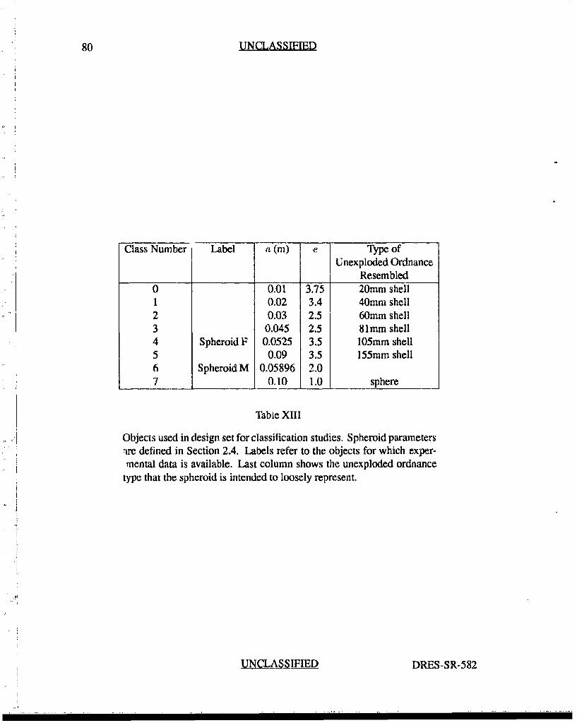
80 UNCLASSIFIED

Class Number Label a (m) e Type ofUnexploded Ordnance

Resembled0 0.01 3.75 20mm shell1 0.02 3.4 40mm shell2 0.03 2.5 60mm shell3 0.045 2.5 81mm shell4 Spheroid F 0.0525 3.5 105mm shell5 0.09 3.5 155mm shell6 Spheroid M 0.05896 2.07 0.10 1.0 sphere

Table XIII

Objects used in design set for classification studies. Spheroid parameters!ire defined in Section 2.4. Labels refer to the objects for which exper-mental data is available. Last column shows the unexploded ordnance

type that the spheroid is intended to loosely represent.

NCLASIFIED DRES-SR-582

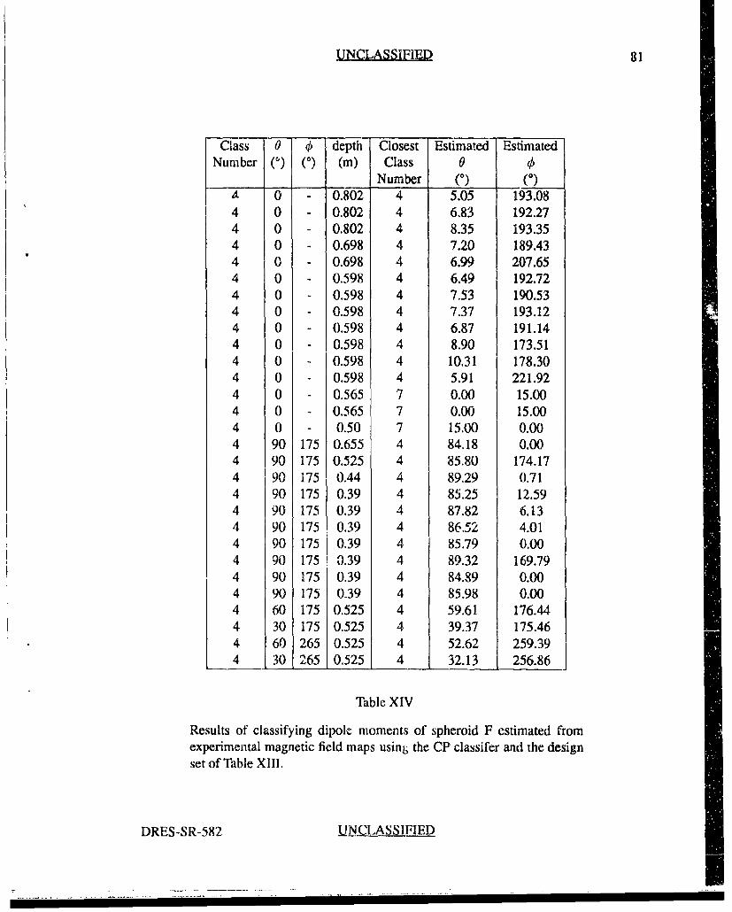
UNCLASSIFIED 81

Class 0 q) depth Closest Estimated EstimatedNumber (m) ( (i) Class 0 0

_Number (0) (0)A 0 - 0.802 4 5.05 193.084 0 - 0.802 4 6.83 192.274 0 - 0.802 4 8.35 193.354 0 - 0.698 4 7.20 189.434 0 - 0.698 4 6.99 207.654 0 - 0.598 4 6.49 192.724 0 - 0.598 4 7.53 190.534 0 - 0.598 4 7.37 193.124 0 - 0.598 4 6.87 191.144 0 - 0.598 4 8.90 173.514 0 - 0.598 4 10.31 178.304 0 - 0.598 4 5.91 221.924 0 - 0.565 7 0.00 15.004 0 - 0.565 7 0.00 15.004 0 - 0.50 7 15.00 0.004 90 175 0.655 4 84.18 0.004 90 175 0.525 4 85.80 174.174 90 175 0.44 4 89.29 0.714 90 175 0.39 4 85.25 12.594 90 175 0.39 4 87.82 6.134 90 175 0.39 4 86,52 4.014 90 175 0.39 4 85.79 0.004 90 175 0.39 4 89.32 169.794 90 175 0.39 4 84.89 0.004 90 175 0.39 4 85.98 0.004 60 175 0.525 4 59.61 176.444 30 175 0.525 4 39.37 175.464 60 265 0.525 4 52.62 259.394 30 265 5 0.525 4 32.13 256.86

Table XIV

Results of classifying dipole moments of spheroid F estimated fromexperimental magnetic field maps usint; the CP classifer and the designset of Table XIII.

DRES-SR-582 UWN._LASLIFIED

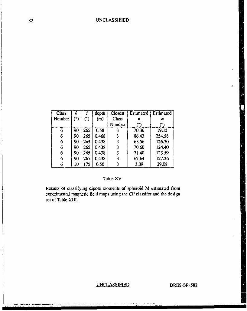
82 UNCLASSIFIED

Class 0 q depth Closest Estimated EstimatedNumber (m) (°) (i) Class 0

Number (0) (0)6 90 265 0.58 3 70,36 19.136 90 265 0.468 3 86.43 254.586 90 265 0.438 3 68.56 126.306 90 265 0.438 3 70.60 124.406 90 265 0.438 3 71.40 123.596 90 265 10.438 3 67.64 127.366 10 175 0.50 3 3.09 29.08

Table XV

Results of classifying dipole moments of spheroid M estimated fromexperimental magnetic field maps using the CP classifer and the designset of Table XIII.

U t.S._IFID DRES-SR.-582

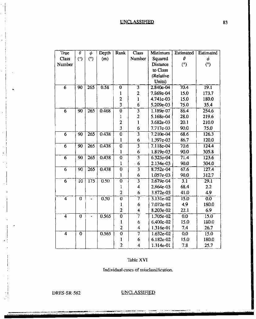
UNCLASSIFIED 83

'True 0 Depth Rank Class Minimum Estimated EstimatedClass (0) (0) (m) Number Squared 0

Number Distance (0) (°)

to Class(Relative

Units)6 90 265 0.58 0 3 2.840e-04 70.4 19.1

1 2 7.869e-04 15.0 173.72 1 4.741e-03 15.0 180.03 6 5.209e-03 75.0 35.4

6 90 265 0.468 0 3 1.189e-07 86.4 254.61 2 5.168e-04 28.0 219.62 1 3.682e-03 20.1 210.03 6 7.717e-03 90.0 75.0

6 90 265 0.438 0 3 7.210e-04 68.6 126.31 6 1.397e-03 86.7 120.0

6 90 265 0.438 0 3 7.118e-04 70.6 124.41 6 1.819e-03 90.0 305.8

6 90 265 0.438 0 3 6.325e-04 71.4 123.61 6 2.134e-03 90.0 304.0

6 90 265 0.438 0 3 8.752e-04 67.6 127.41 6 1.057e-03 90.0 312.7

6 10 175 0.50 0 3 2.679e-04 3.1 29.11 4 2.864e-03 68.4 2.22 6 3.872e-03 41.0 4.9

4 0 - 0.50 0 7 3.131e-02 15.0 0.01 6 7.072e-02 4.9 180.02 4 8.203e-02 22.1 6.9

4 0 0.565 0 7 1.705e-02 0.0 15.01 6 .400C-2. I 15.0 10.0

2 4 1.316e-01 7.4 26.74 0 0.565 0 7 1.632e-02 0.0 15.0

1 6 6.182e-02 15.0 180.0- -- 2 4 1.314e-01 7.8- 25.7

Table XVI

Individual cases of misclassification.

DRES-SR-582 N CLAS, FED

ON

84 UNCLASSIFIED

U

U.NCLASSIFIED DRES-SR-582

UNCLASSIFED 85

7. Conclusions

An improved "smart" microprocessor controlled magnetometer which can accuratelylocate and identify compact ferrous objects in real-time has been described. The instrument,which is person-portable, consists of a cesium vapour magnetometer mounted on a cart witha wheel-mounted optical encoder, a microcontroller, interface and a laptop computer. Theinstrument guides the operator in the collection of simultaneous magnetic field and positiondata in a horizontal plane above an object. Location is estimated by applying a custom-made noniterative location estimation algorithm to the data. A byproduct of the locationalgorithm is an estimate of the dipole moment which is used by a continuous parameterpattern classifier to identify the object. With the present instrument, 6 to 13 minutes arerequired to collect the data, location and dipole moment estimation requires 5 seconds andclassification requires 30 seconds.

Detailed experiments were performed using two different ferrous spheroids, similar inshape to unexploded ordnance, in order to determine limits of error in estimation of thelocation and the dipole moment and the error in classification.

The precision in estimating location varied from 0.12 to 1.35% of the depth for a fixedobject and orientation at a given depth. There was a slight variation in location estimate withobject type and/or orientation which increased the location uncertainty to 1.67 to 1.90% ofthe depth. The precision in estimating the dipole moment varied from 0.51 to 8.21 % of thedipole moment magnitude. There was a slight increase in uncertainty as depth decreased,but the precision was not closely correlated with peak magnetic field.

All three components of the location estimate had a depth dependent bias which waslarger than can be accounted for by the precision of the estimation. The X01 componentof the location was almost always overestimated. The Xo2 component was generallyoverestimated for depths less than 0.55 m and underestimated for depths between 0.55in and 0.8m. A similar trend appeared to occur for the X 03 component except that thecrossover from overestimation to underestimation occured at about 0.45 m depth. Errors inX03 were generally larger than those for XoI and X02, the root mean square (rms) error overall depths being G.)20 m for X01 , 0.019 m for Xo2 and 0.045 m for X03. By comparison,the average precision for a fixed object and orientation was 0.005 m for X01, 0.003 m forX02, and 0.004 to for Xo3.

There was a deviation between theoretical values and experimental estimates of the

DRES-SR-582 U SSI.I

"" -_...._ _ _ --- -I..•••• -,-"-••g.-•••-•-••

86 UNCLASSIFIED

dipole moment that was greater than the uncertainties in the estimates. The unweightedaverage difference between estimated and theoretical dipole moment components as apercentage of the theoretical dipole moment was 4.8 ± 7.6% for M1, -3.3 ± 15.5% forAl2, -10.8 ± 17.5% for M3 and 24.5 ± 11.4% for the magnitude of the vector difference.There was no clear trend with object type, orientation or depth.

Following quantification of the error in the estimation of location and dipole moment,sources of error and their relative effects were analysed. It was argued that a substantialfraction of the uncertainty (precision) in dipole location and moment vector estimates wasdue to positional uncertainty in the experiments.

By applying the location algorithm to magnetic total field data generated by computerusing a mathematical model based on magnetization induced in spheroids by a uniformmagnetostatic field, the effects of remnant magnetization and positional uncertainty couldbe eliminated. It was shown that the estimation error of the location vector was roughlyindependent of whether the magnetic field data was experimental or computer generated.Dipole moment estimation errors for computer generated data were slightly smaller thanthose for experimental data. This suggested that positional error in these experiments hadlittle influence on location and moment vector estimation and that remnant magnetizationin the spheroids must be small compared to the induced magnetization. It was shown thatthe finite volume of the sensor head was not a significant source of error for the geometryof these experiments. A variation of error with depth and object orientation was noticedfor the computer generated data. This suggested that the main contributor to the error wasestimation of the position of the field extrema and the use of total field in place of verticalcomponent magnetic data.

The location algorithm was applied to magnetic vertical component field data generatedfrom the computer model in order to determine how much of the error in estimation was dueto using total field measurements to approximate the vertical component of the magneticfield. Since the bias in estimation of the sphere for vertical component data was roughly2 to 6% of the moment magnitude, whereas for total field data it was 20%, this suggestedthat the error due to the total field approximation varied from 14 to 18% of the momentmagnitude. It was estimated that the error due to estimation of extrema positions and higherorder moments varied from 0 to 8% of the moment magnitude.

The analysis of error in the computer generated total magnetic field data allowed limitsto be set on the misclassification rate that can ultimately be attained. The moment estimatesfor a given object and orientation were found to vary by between 2 and 4% of the momentmagnitude as the depth varied. If the estimated moments were used in the design set, thissuggests that the limiting misclassification error would be between roughly 1.4 and 2.4%if the experimental (mainly posizional) error were substantially less than the algorithmicand approximation errors. For •he present experimental precision (4.1 ± 3.0% ), themisclassification error should be roughly between 2 and 5% (assuming quadrature errorsummatiot) if the design set were experimentally obtained.

Pattern classification was performed with a computer generated dipole moment design

UNCLASSIFIEID DRES-SR-582

UNCLASSIFIED 87

set consisting of 8 objects including the 2 used in these experiments. The gross misclas-sification rate was 10.3% for the class number 4 spheroid and 100% for class number 6.Closer examination revealed that class 6 was always classified as class number 3, which is asimilarly shaped spheroid. This is likely due to the deviation between the moment estimatesfor the experimental spheroid and the computer model. The repeatability of classification,that is, the percentage of cases in which an object is classified as the same class, is a bettermeasure of classifier performance. The repeatability of classification was 91.7%. If weconsider only the two objects for which experimental measurements were made, we seethat only 4/36 cases (11 .1 %) were classified incorrectly.

The overall performance of the smart magnetometer is very encouraging, but additionalstudies need to be performed. Although remnant magnetization has been shown to besmall in these and previous experiments, this must be verified by estimating momentsfor sets of identically shaped spheroids at fixed depths. This should also be repeated forunexploded ordnance. The possibility of accurately determining the relative contributionsof remnant and induced mLgnetization should be investigated. A major source of error isthe estimation of position of the magnetic field extrema. A possible improvement is toregularize the sampling grid for the magnetic field measurements so that two dimensionalinterpolation may be used to estimate the extremum position, rather than its ceotroid as iscurrently done. This appproach, which will be investigated, may improve the accuracy ofthe peak position estimates. The possibility of applying corrections to the total field data toimprove its approximation to vertical component data should be investigated. One possiblemethod to achieve this might be to use a three sensor orthogonal axis fluxgate total fieldmagnetometer which is either on a stabilized platformi or whose orientation angles withrespect to a fixed coordinate system are known. Whether such a system is practical mustbe investigated. Most importantly, a comprehensive design set must be assembled frommeasured experimental magnetic field maps of objects of interest.

The last proposed study will require considerable time, given that between 6 and 13minutes are required to collect the data for one dipole moment estimation. This laboratory,in conjunction with Pylon Electronics Ltd. of Ottawa, Canada, is presently developing amultisensor fluxgate gradiometer which will incorporate a modified Wynn-Frahm locationalgorithm [16] and the present pattern classifier. The gradiometer will be able to estimatelocation from a single measurement in space and hence sufficient data for a momentestimation will be collected,.• in 'less than a second. To use a design set from the gradiometerin the magnetometer, the estimated dipole moments from one instrument must be nearlyequal to those from the other. A comparative study of the dipole moment estimation errorsfor both the smart magnetometer and gradiometer will be conducted using the spheroidmodel, and later using real magnetic field and field gradient data.

DRES-SR-582 UNCLASSIFIED

88 UNCLASSIFIED

I

.MNCi 4 •El•L DRES-SR-582

UNCLASSIIED2 89

8. Referencest

l1] R.Robert.on. UNDEX site survey report (U). Report TR-303, Naval ExplosiveOrdnance Disposal Technical Center, Indian Head, MD, USA, September 1991. UN-CLASSIFIED.

[2] J.E.McFee and Y.Das. Determination of the parameters of a dipole by measurement ofits magnetic field. IEEE Transactions on Antennae end Propagation, AP-29:282-287,March 1981.

[3] J.M.Stanley and M.K.Cattach. An image processing magnetometer system for explo-sive crunance detection. Report, Geophysical Research Institute, University of NewEngland, Armisdale, NSW, Australia, 1989.

[41 Institut Dr. Forster. FEREX CAST 4.021.06 computer aided search technique to loc. teferrous-metal objects. Sales Brochure, 1991. Prufgeratebau GmbH, Unternchmens-bereich, Spezialprodukte, Postfach 15 64, D-7410, Reutlingen, Germany.

[5] Aprotec Ltd. CAMAD. Sales Brochure, c6rca. 1986. Enterpr•se House, ManchesterScience Park, Lloyd Street North, Mancheser, M15 4EN, England.

[61 J.E.McFee, Y.Das, and R.Ellingson. Locating and identifying compact ferrous objects.IEEE Transactions. on GeoScienre and Remote Sensing, GE-28(2):182-093, March1990.

[71 J.E.McFee, M.Bell, B.Dempsey, R.Chesney, and Y.Das. A magnetostatilc signaturemeasurement and analysis system. Journal of Physics E, 18:54-60, January 1985.

[81 J.E.McFec and Y.Das. A multipole expansion model for compact ferrous objectdetection. In Proceedings of the ,41NTEM Symposium on Antenna Technology andApplied Electromagnerics, pages 633-638, University of Manitoba, Winnipeg, MN,Canada, August 1990.

191 J.E.McFee. Electromagnetic remote sensing - low frequency clectromagnetics (U).Special Report SSPI124, Defence Research Establishment Suffield, January 1989.UNCLASSIFIED.

DRES-SR-582 UNCLASStIFED

90 UNCLASSIFIED

[10] J.E.McFee and Y.Das. Fast nonrecursive method for estimating location and dipolemoment components of a magnetic dipole. IEEE Transactions on GeoScience andRemote Sensing, GE-24:663-673, September 1986.

111] J.E.McFee and Y.Das. A classifier for feature vectors whose prototypes are a functionof multiple continuous parameters. IEEE Transactions on Pattern Recognition andMachine Intelligence, PAMI-10:599--606, July 1988.

[12] J.Stratton. Electromagnetic theory. McGraw-Hill, New York, 1941.

[13] Scintrex Limited, Concord, Ontario, Canada. ViO0 Portable cesium high-sensitivitygradiometer system.

[141 Motorola, Motorola Literature Distribution, Phoenix, AZ. MC68332 user's manual,MC68332UM/AD edition, 1990.

[15] J.T.Tou and R.C.Gonzalez. Pattern recognition principles. Addison-Weslcy, ReadingMassachusetts, 1974.

116] W.Wynn, C.Frahm, P.Carroll, R.Clark, J.Wellhoner, and M.Wynn. Advanced super-conducting gradiometer/magnetometer arrays and a novel signal processing technique.IEEE Transactions on Magnetics, MAG- 11:701-707, 1975.

D

11iLSSJIFID DRES-SR-582