Embed Size (px)
Citation preview
SEUIYCLASSIFICATION OF ii
U NCIrC v , r AD-A263 049lREPORT SECURITY CLASSIFICATION iuUu IUnclassified11 1 1 1 1
SECURITY CLASSIFICATION .**.-.."*.-- OP.- R~EPORT
Ng r - -Aprro.~
2b. DECLASSIFICATION / DOWN Li & Li1 di:2 ?
4, PERFORMING ORGANIZATIO FIT NUM[;5) 5 MONITORiNG ORGANIZATION REPORT NUMBER.iSý
AFOSRTR- ('I~ )j~
6a. NAMPS RFORUING ORGANIZATION 6b OFFICE SYMBOL 74 NAME OF MONITORING ORGANIZATIONDe~t.'oF Aeronautics and (if Apoi.cablit
Astrnauics31-24 Se ~ AFOSRINAAstronautics ________ 31_204________ BolliaS AF3 flC ?033?-644Ft
6C. ADDRESS (CitY, State, and ZIP Code) 70~ ADDRESS (City, Statre, and lip Coop)
77 Massachusetts Ave. e4 AORNCamnbridge, MA 02.139
5 ef FSfI8 o ! i 3 A 2%'222- 6 14S
8.. NAME OF FUNDING ISPONSORING 180 OFFICE PYM9L 9 PROCOREMENT INSTRUMENT IDENTIFCATION NuMS(ItORGANIZATION ( 14 J~I~bef
AEOSP I "Kil10- Grant AFOFI-90-1'035
8c. ADDRESS (City. State. and ZIP Code) 10 SOURCE OF FUNDING NUMBERSAORPROGRAM PtOJECT' TASK~ WORK UNITAFSRýEMVENT NO INO fO3ACESINN
Boilinp AFB. DC 20332 a 11cO JCESIN Y
11 TITLE (include Security Classification)
Unsteady Flow Phenomnena in Turbomachines
1ýNT AePA Epstein M-B. -CGies . Ji. .. McCune C.ý. 'an
±~r9 ~~a 13b TIME ýCVE.RE D 114 DATE OF REPýýT lfylh Day) SRtý ONAA FfRn?~lOMI' 3 289 TO 10 /1 9 /92 January vI ~l, ~ .ON
16, SUPPLEMENTARY NOTATION
17 COSATI CODES 18 SUBJECT TERMS (Continue on reverie if necessary and identify by block number)
FIELD GROUP SUS.GRO-UP Connutational Fluid Mechanics tnsteadv rlows ir Thrbo-machines Vortex Vakes. Comnressor ctabilit- "ransonicCompressors
19. ABSTRACT (Continue on reverse if necessary and identify by block number)
This renort describes work carried out at the Gas Turbine Laboratorl" at MIT duringý the
period 10/20/89 - 10/19/92, as Part ol our multi-investio~ator effort on has~c unstead-
f low Phenomena in turbomacfllnes. W~ithin the overall nroiect 1our senarate tasks are
specified, These are. in brief: 1. The Influence ol Inlet Temnerature Nonuni'formitles
on Turbine Heat Transfer and Dynamics; IT. Assessment of Unsteady Losses in 5'tator/
Rotor Interactions; Ill. Unsteady Phenomena and Flowfield Tn~stahilities in Miultistaqe
Axial Compressors; IV. Vortex Wake-Compressor Blade Interaction in Cascades: A New
jPapid Me~tlod for Unsteady Separation and Vorticity Flux Calculations.
93 31 067 93-06629
00 FORM 1473.64 MAR 83 APR editionl may be used untitl exhausted SECURIT CLASSIFICATION OF ýHIS PAGE
All ~~C Lte Ddt~sae b~eg

Gas Turbine LaboratoryDepartment of Aeronautics and Astronautics
Massachusetts Institute of TechnologyCambridge, MA 02139
Final Technical Report
on
Grant AFOSR-90-0035
entitled
UNSTEADY FLOW PHENOMENA IN TURBOMACHINES
for the period
October 20, 1989 to October 19, 1992
submitted to
AIR FORCE OFFICE OF SCIENTIFIC RESEARCHBuilding 410
Boiling Air Force Base, DC 20332
Attention: Major D. Fant
mtre Q M sn=4'
PRINCIPALINVESTIGATOR: Edward M. Greitzer Acceson For
H.N. Slater Professor and De AcSo oRAGas Turbine I.aboratory NTIS CRA&Bortic rAs EJ
CO-INVESTIGATORS: Professor Alan H. Epstein UvannouncedJusstiihction
Professor Michael B. Giles .Professor James E. McCune ByDr. Choon S. Tan Distributlon/
January 1993 Availability Code%Avail aodtor
ODst Special
ý\A

I
TABLE OF CONTENTS
Sectio patN
1. Introduction and Research Objectives 2
2. Status of the Research Program 3
Task I: The Influence of Inlet Temperature Nonuniformniieson Turbine Heat Transfer and Dynamics 3
Task II: Assessment of Unsteady Losses in Stator/Rotor Interactions 97
Task 1II: Unsteady Phenomena and Flowfield Instabilitiesin Multistage Axial Compressors 119
Task IV: Vortex Wake-Compressor Blade Interaction in Cascades: A New
Rapid Method for Unsteady Separation and Vorticity Flux Calculations 155
3. Air Force Research in Aero Propulsion Technology (AFRAPT) Program 170
4. Publications and Presentations 172
5. Program Personnel 173
6. Interactions 174
7. Discoveries, Inventions, and Scientific Applications 178
8. Concluding Remarks 179

1. INTRODUCTION AND RESEARCH OBJECTIVES
This is a final technical report on work carried out at the Gas Turbine Laboratory at MIT, in a
multi-investigator effort on unsteady flow phenomena in turbomachines. Support for this
program was provided by the Air Force Office of Scientific Research under Grant Number
AFOSR-90-0035, Major D. Fant, Program Manager.
The present report gives a imnw= of the work for the period 10/89 - 10/92, but is not
intrnded to be the primary wurce and the refereiwed reports and publications can be consulted for
more detailed information and background. These describe the research in considerable depth.
Within the general area of turbomachinery fluid dynamics, four separate tasks were specified
under this contract. These are, in brief:
I. The influence of inlet temperature non-uniformities on turbine heat transfer and
measurement.
II. Development and application of computational techniques for unsteady flows and
assessment of unsteady losses in rotor/stator interactions.
III. Unsteady phenomena, inlet distortion and flow instabilities in multistage compressors,
including experimental and analytical investigations of the structure of instability
precursors, nature of rotating stall modes, and detailed blade passage aerodynamics and
stall onset in advanced blading geometries.
IV. Unsteady blade-vortex street interaction in transonic cascades including models to describe
the vortex wake-compressor blade interactions.
In addition to these tasks, the multi-investigator contract encompassed the Air Force
Research in Aero Propulsion Technology (AFRAPT) Program. The work carried out in each of
the tasks will be described in the next section. Publications generated are given in the individual
task descriptions, and an overall list of presentations and publications associated with the projects
appears in Section 4.

3
TASK I: THE INFLUENCE OF INLET TEMPERATURE NONUNIFORMITIESON TURBINE HEAT TRANSFER AND MEASUREMENT(Investigators: A.H. Epstein, G.R. Guenette, T. Shang, M. Graf)
1.0 Executive Summary
This is a technical progress report on the research conducted on the turbine inlet
temperature distortion cooperative research program through December 1992. The objectives of
the program are to elucidate the role of inlet temperature nonuniformity and turbulence on turbine
rotor heat transfer through detailed experiments and calculations. The sponsors are SNECMA,
Rolls-Royce, Inc., US Air Force Office of Scientific Research, and NASA Lewis Research Center.
The effort is focused about a set of experiments on the MIT Blowdown Turbine facility in which
the effects of inlet temperature distortion on a transonic turbine stage will be directly measured.
This data will then be compared with CFD and analytical results.
The activities to date have concentrated on the refurbishment of the test rig, the addition of
turbulence grids, the upgrading of heat transfer and aerodynamic instrumentation, the adaptation of
a 3-D, inviscid, unsteady code to the measurement geometry, final assembly of the aerodynamic
instrumentation and its calibration, initial NGV-only testing, and the resolution of problems
encountered during the initial tests. The test rig refurbishment includes cleaning of the temperature
distortion generator and reconfiguration of the generator to simultaneously produce different radial
and circumferential distortion in separate 120 sectors.
Instrumentation upgrading consists of reinstrumentation of the rotor blades with heat flux
transducers, the addition of circumferential rake translators upstream and downstream of the
turbine, and the design and construction of pressure and temperature rakes for the translators. The
tempemture instrumentation measures time-averaged total temperature, while both time-averaged
and time-resolved rakes were fabricated for total pressure. Wall static pressure taps have been
added at the inner and outer annulus wall downstream of both the NGV's and the rotor. New
signal conditioning and data acquisition equipment to accommodate the 80 additional aerodynamic
measurement transducers has also been procured or constructed.

The temperature and pressure rakes were assembled and calibration. Considerable noise
and induced signals were observed on the exit temperature rake during traverse shakedown in
vacuum. This problem was solved with an improved grounding scheme. The overall DC
accuracy and stability appear to be within 0.2%, sufficient for the planned test program.
The instrumentation performed as designed during the first NGV-only blowdown tests.
The inlet rake mapped the distortion generator exit flowfield and the turbine exit rake could readily
resolved the NGV wake structure. During the first test, cabling from the turbine exit translator
became entangled in it drive chain. The exit cabling arrangement was modified to resolve this
problem.
Turbulence screens have been designed and fabricated which match the turbulence
spectrum suggested by Rolls-Royce as being representative of engine scale. These screens have
been tested in a wind tunnel with satisfactory results.
A 3-D, unsteady, Euler code written by Saxer and Giles is being adapted to the test
geometry. The code will be run with three NGV's and five rotor passages to simulate the 36
NGV, 61 rotor blade count of the experiment.
Two problems were encountered with the temperature and distortion generator -
inadequate circumferential distortion and particulate contamination. The low level of
circumferential distortion achieved was traced to the storage matrix having 15 times more thermal
conductivity in the circumferential direction compared to the radial one, due to poor fabrication.
This has the effect of quickly washing out circumferential distortions. The approach adopted was
to double the number of spot heaters and run them at very high current levels Oust below burnout
as established experimentally) immediately preceding the blowdown tests. The particle
contamination of the distortion generator has been a continuing problem and efforts to clean the
unit have not been successful. The approach adopted here was to fabricate and insert a particle
filter at the distortion generator exit.
An operational problem has developed due to the ten-fold increase in the price of Freon- 12,
to about $1200 per test - well beyond the budget. We plan on using Freon for the first tests only

5
for continuity and then converting to an argon-CO- gas mixture.
The current schedule is to do the NGV-only testing in January and start the full-stage
testing in February 1993.
2.0 Jntrnuiin
The objective of this work is to understand how turbine inlet distortion and turbulence
influence turbine heat transfer and aerodynamics. It is centered on a set of detailed spatially and
temporally resolved measurements of a high pressure ratio turbine stage in a short duration turbine
test facility. Numerical simulauon and analytical modelling will then be used to interpret these
measurements and help draw conclusions of use to a turbine designer.
The experimental work will be carried out in the MIT Blowdown Turbine Facility. This rig
can simulate all of the non-dimensional fluid mechanic parameters known to be important in
turbine aerodynamics (Reynolds No., Rossby no., Mach No., gas-metal temperature ratios, Prandtl
No., ratio of specific heats, etc.) for approximately 300 ms. Turbine corrected speed and weight
flow are held constant to better than 0.5% over this period. During the test, approximately 20
million data points can be taken from a variety of heat transfer and aerodynamic instrumentation.
The program plan is to setup a temperature distortion generator to produce both
circumferential (hot spots) and radial temperature distortions simultaneously in separate 1200
sectors. The time resolution of the instrumentation will permit differentiation among the sectors.
The test plan for this year is to first operate the tunnel without the rotor so as to permit
aerodynamic mapping of the nozzle guide vane (NGV) exit flowfield. (Since the nozzles are
choked, the flowfield may approximate that with the rotor in place.) The rotor will then be added
and the heat transfer and stage aerodynamic data taken.
To date, the effort has concentrated on readying the facility and its instrumentation for these
tests, and adaptation of numerical tools. For the sake of this report, we will divide this effort into
categories - (1) facility refurbishment and addition of inlet and outlet rake translators; (2) design
and testing of turbulence grids; (3) new aerodynamic instrumentation and signal conditioning

6
equipment; (4) new rc,tor blade heat flux instrumentation; (5) CFD code adaptation and checkout;
(6) instrumentation preparation and calibration; (7) NGV-only testing; and (8) problems uncovered
and their solutions. In the following sections, we examine each item in turm.
3.0 Facility Refurbishment and Modification
Three major items are required to ready the facility for the distortion testing -
refurbishment of the facility, cleaning and retrofitting of the distortion generator, and the addition
of new upstream and diwnstream circumferential translation capability. The tunnel refurbishment
consists of disassembly; cleaning; bearing, seal, and lubricant replacement; etc., as well as
checkout of the control, heating, eddy brake, and safety systems.
3.1 Distortion Generator
The distortion gen,:rator was cleaned and reconfigured. The unit (0.5 m dia. x I m long)
was cleaned in an ultrasonic cleaner to remove the particles which caused extensive
instrumentation damage during the previous test series. These appeared to be 25 pin diameter,
clear particles, probably silica from grit blasting at the honeycomb manufacturer. The unit was
cleaned repeatedly, the cleaning fluid filtered, and the particle number noted. The number of
particles was reduced on each cleaning until none remained.
The heaters from one of three radial distortion sectors of the generator was removed and
the unit rethreaded as a circumferential distortion generator (Fig. 1). In this segment, the heaters
are 6 mm in circumferential extent and spaced 2 nozzle guide vane pitches apart to approximate
combustor nozzle spacing. Thirty thermocouples measuring metal temperature were then spotted
about the matrix to aid in pre-test setup. The heaters and thermocouples performed satisfactorily in
air. The generator is ready to go.
Different temperature patterns will be generated by varying the time temperature history of
the wire heaters. High currents for short times will generate "spiky" distortions, which will soak
out over time, lessening the temperature modulation. This is illustrated conceptually in Fig. 2. As
an aid in the setup of the patterns, a numerical conduction model of the generator is being written
7
and will be fit to the experimental data.
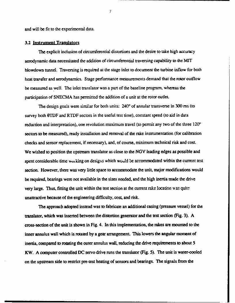
3.2 Instrument Translators
The explicit inclusion of circumferential distortions and the desire to take high accuracy
aerodynamic data necessitated the addition of circumferential traversing capability to the MIT
blowdown tunnel. Traversing is required at the stage inlet to document the turbine inflow for both
heat trarsfer and aerodynamics. Stage performance measurements demand that the rotor outflow
be measured as well. The inlet translator was a part of the baseline program, whereas the
participation of SNECMA has permitted the addition of a unit at the rotor outlet.
The design goals were similar for both units: 2400 of annular transverse in 300 ms (to
survey both OTDF and RTDF sectors in the useful test time), constant speed (to aid in data
reduction and interpretation), one revolution maximum travel (to permit any two of the three 120O
sectors to be measured), ready installation and removal of the rake instrumentation (for calibration
checks and sensor replacement, if necessary), and, of course, minimum technical risk and cost.
We wished to position the upstream translator as close to the NGV leading edges as possible and
spent considerable time w,,dng on desigiis which would be accommodated within the current test
section. However, there was very little space to accommodate the unit, major modifications would
be required, bearings were not available in the sizes needed, and the high inertia made the drive
very large. Thus, fitting the unit within the test section at the current rake location was quite
unattractive because of the engineering difficulty, cost, and risk.
The approach adopted instead was to fabricate an additional casing (pressure vessel) for the
translator, which was inserted between the distortion generator and the test section (Fig. 3). A
cross-section of the unit is shown in Fig. 4. In this implementation, the rakes are mounted to the
inner annulus wall which is rotated by a gear arrangement. This lowers the angular moment of
inertia, compared to mating the outer annulus wall, reducing the drive requirements to about 5
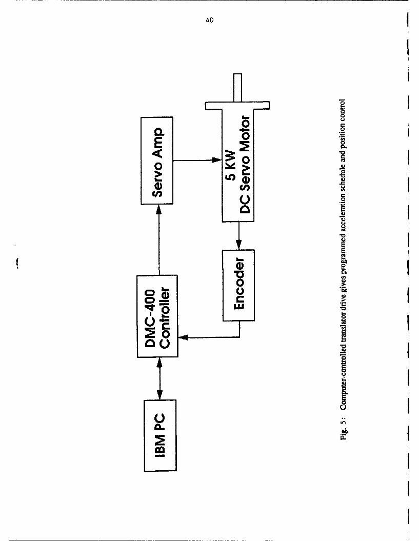
KW. A computer controlled DC servo drive runs the translator (Fig. 5). The unit is water-cooled
on the upstream side to restrict pre-test heating of sensors and bearings. The signals from the

8
transducers are brought out of the rotary system by coiled wires (thus the one revolution
maximum travel) and out of the pressure vessel by a vacuum feedthrough. A measured time trace
of the translator motion is shown in Fig. 6. The unit operates satisfactorily.
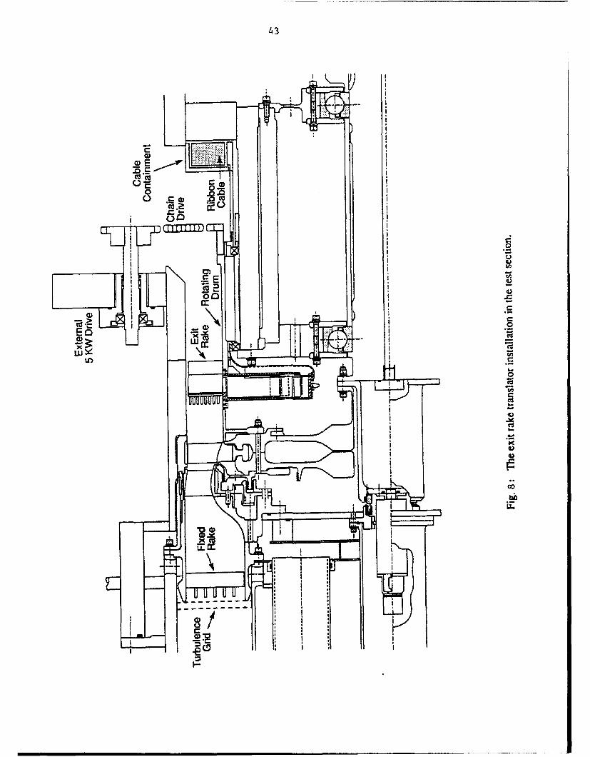
The rotor exit translator was a much more difficult task in that there was no choice but to fit
it within the existing test section and the geometric constraints are severe. In this case, the deswirl
vanes downstream of the rotor are replaced by the translator. The tunnel flow path is shown in
Fig. 7, while the detail of the translator is given in Fig. 8. As for the upstream translator, the
probes are mounted on the inner annulus flow path wall. This wall is mounted on thin line
bearings and chain-driven (the chain is in the flow path). The ribbon cabling is used which is
formed into a spring coil under the turbine exit throttle sleeve. A DC servo drive similar to the
upstream unit is used with the addition of a gearbox to increase the torque. As of this date, the unit
has performed satisfactorily mechanically. The instrumentation wiring has not been completed.
4.0 Turbulence Generation
The influence of turbulence on rotor heat transfer will be explored by operating the facility
with high and low levels of turbulence. The blowdown turbine naturally produces a very quiet in-
flow, with turbulence levels measured before the contraction into the NGV's of less than I%.
Engine levels are considerably more, and we must ask the question "What are appropriate
intensities and scales?" Rolls-Royce has suggested that the work of Moss and Oldfield [I] is a
suitable representation of engine conditions. We have been operating under this assumption in the
work described below. More recently, at the April program review and in subsequent
correspondence, Dr. Richard Rivir of the USAF Wright Laboratories has pointed out that his work
shows considerably more energy at high spatial frequencies than does that of Moss and Oldfield.
We are in the process of trying to understand this discrepancy and would appreciate the opinions
of our partners.
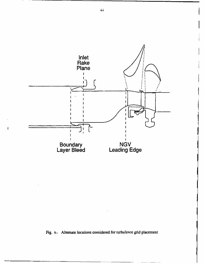
Basing the design criteria on Moss and Oldfield data, we considered the suitability of grids
to produce the desired spectrum. Meshes placed at two axial stations were considered: (1) at the
9
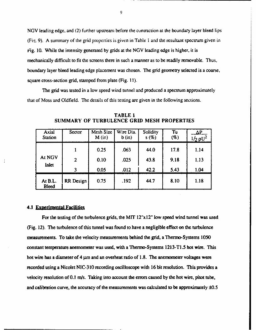
NGV leading edge, and (2) further upstream before the contraction at the boundary layer bleed lips
(Fig. 9). A summary of the grid properties is given in Table I and the resultant spectrum given in
fig. 10. While the intensity generated by grids at the NGV leading edge is higher, it is
mechanically difficult to fit the screens there in such a manner as to be readily removable. Thus,
boundary layer bleed leading edge placement was chosen. The grid geometry selected is a coarse,
square cross-section grid, stamped from plate (Fig. 11).
The grid was tested in a low speed wind tunnel and produced a spectrum approximately
that of Moss and Oldfield. The details of this testing are given in the following sections.
TABLE ISUMMARY OF TURBULENCE GRID MESH PROPERTIES
Axial Sector Mesh Size Wire Dia. Solidity Tu APStation M (in) b (in) s (%) (%) 1/2 pU2
1 0.25 .063 44.0 17.8 1.14
At NGV 2 0.10 .025 43.8 9.18 1.13
Inlet3 0.05 .012 42.2 5.43 1.04
At B.L. RR Design 0.75 .192 44.7 8.10 1.18Bleed I _ _ _ _ _ _
4.1 Experimental Facilities
For the testing of the turbulence grids, the MIT 12"x12" low speed wind tunnel was used
(Fig. 12). The turbulence of this tunnel was found to have a negligible effect on the turbulence
measurements. To take the velocity measurements behind the grid, a Thermo-Systems 1050
constant temperature anemometer was used, with a Thermo-Systems 1213-TI .5 hot wire. This
hot wire has a diameter of 4 .im and an overheat ratio of 1.8. The anemometer voltages were
recorded using a Nicolet NIC-310 recording oscilloscope with 16 bit resolution. This provides a
velocity resolution of 0.1 m/s. Taking into account the errors caused by the hot wire, pitot tube,
and calibration curve, the accuracy of the measurements was calculated to be approximately ±0.5

101
m/s.
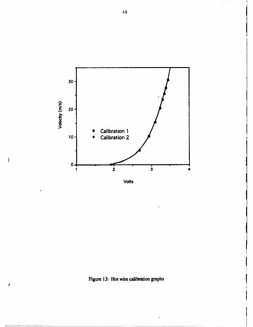
The calibration of the tunnel was done using a pitot tube attached to a pressure transducer.
The pitot tube also acted as a check on the accuracy of the hot wire during the tests. The calibration
curve of anemometer output voltage versus velocity was then used to convert the test voltages to
velocities. Although the tunnel was calibrated at the beginning of each test sequence, the drift of
the calibration curve was checked to see if it would produce an appreciable error as the tests
continued. Figure 13 shows that the curve remains approxima-ely constant with time.
Two groups of tests were carried out in the tunnel. The first group measured the
turbulence characteristics at a position half way between the turbulence grid and nozzle guide
vanes, and at the position of the nozzle guide vanes. At these two streamwise locations, six
measurements were taken at different transverse positions to the flow to check for changes in
turbulent characteristics in the transverse direction. The object of this first group of tests was to
compare the results with similar tests run in the past [2], to confirm the grid was producing the
correct turbulent characteristics.
For the second half of the tests, a plexiglass nozzle section was added to the tunnel. This
nozzle is the same dimensions as the nozzle section in the blowdown turbine facility. The
locations of the test positions was the same as for the first half of the tests. With these results, the
freestream turbulence characteristics entering the nozzle guide vanes is known for the blowdown
turbine facility. These turbulence characteristics can then be compared with measurements from a
typical gas turbine engine burner exit.
4.2 Dlata.Anal
When looking at the effect of turbulence on rotor heat transfer, it is found that two of the
most important parameters whi-h characterize turbulence are turbulence intensity, and the power
spectral density. The turbulence intensity is defined as
Tu=- u

!1
The power spectral density, relating turbulent energy with wave number, can be found by
squaring the finite fourier transform of the data (see Table 2). From the data, the one sided power
spectral density can be found as follows
G(k) = 1 iX(f)l2
nUNAt
where
N-1
X(f) = At I u'(n)e-i2xfnAt nn-O
TABLE 2NOMENCLATURE
f Frequency (Hz)
u Velocity fluctuation (m/s)
U Mean axial velocity (rm/s)
k Wavenumber (/rm) = 2xf/U
G(k,U) One-sided power spectral density = d(u'fU)/dk
Tu Turbulence Intensity
N Number of samples = 4000
At Time between sampling points (s)
X(f) Fourier transform
A Integral length scale
For the first half of the experiments, these calculated values for turbulerwe intensity and
power spectral density can be compared with similar tests performed in the past 12]. From these
past experiments, the turbulence intensity and power spectral density were found to be
approximated by
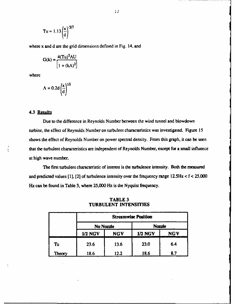
Tu = 1.1 x3~
where x and d are the grid dimensions defined in Fig. 14, and
G(k) = 4(Tu)2AU
I I + (kA)2]
where
A =0.2d()
4.3 Rj~Il
Due to the difference in Reynolds Number between the wind tunnel and blowdown
turbine, the effect of Reynolds Number on turbulent characteristics was investigated. Figure 15
shows the effect of Reynolds Number on power spectral density. From this graph, it can be seen
that the turbulent characteristics are independent of Reynolds Number, except for a small influence
at high wave number.
The first turbulent characteristic of interest is the turbulence intensity. Both the measured
and predicted values [1], [2] of turbulence intensity over the frequency range 12.5Hz < f < 25,000
Hz can be found in Table 3, where 25,000 Hz is the Nyquist frequency.
TABLE 3TURBULENT INTENSITIES
Streamwlae Position
No Nozzle Nozzle
1/2 NGV NGV 1/2 NGV NGV
Tu 23.6 13.6 23.0 6.4
Theory 18.6 12.2 18.6 8.7

13
From Table 3, it can be seen that the measured values of turbulence intensity were higher than the
predicted values, except at the NGV streamwise location with the nozzle installed. This is the
position of importance, because this position corresponds to the position of interest in the
blowdown turbine facility. At this position, the measured value of turbulence intensity was lower
than the turbulence intensity that would occur at this position in a typical gas turbine engine.
The other turbulence characteristic of importance is the power spectral density. Figures 16
and 17 show the graphs of the power spectral density for the no nozzle case at the 1/2 NGV and
NGV streamwise locations respectively.
These two figures show the measured values of turbulent energy at high wavenumber
correspond nicely with theory, while the measured energy at low wave number is noticeably
higher than predicted. A series of tests were run in which a low pass filter was used to filter out
the high frequency contribution of energy to the power spectral density to show that this high
energy level at low wavenumber was not caused by aliasing of the signal when the data was taken.
In Fig. 18, the graph of the power spectral density at the NGV streamwise location is plotted with
the nozzle installed.
In Fig. 18, the theory line [1] is measurements taken at the burner exit of a simulated gas
turbine combustor. The turbulence energy measured in the wind tunnel matches the turbulence
energy measured in the gas turbine rather well at high and low wavenumber, however the wind
tunnel measurements of turbulence energy are noticeably lower in the intermediate wavenumber
region. This lower energy region agrees with the lower value of turbulence intensity measured in
the wind tunnel.
In order to check the effect of transverse positioning of the hot wire on turlence
characteristics, a number of measurements were carried out at various Muansverse positions, while
keeping the streamwise position constant. The measurements were taken at the NGV streamnwise
position, with nozzle installed. Figure 19 shows the effect of transverse positioning in the direction
parallel to the nozzle by looking at two positions 1/2 of one grid mesh apart in the direction parallel
to the nozzle. Figure 20 shows the effect of transverse positioning in the direction of nozzle

141
contraction by looking at two positions 1/2 of one grid mesh apart in the direction of nozzlecontraction.
Figure 19 shows that the parallel positioning of the hot wire in the nozzle has little effect on
turbulence characteristics, while Fig. 20 shows that hot wire position has a considerable effect in
the direction of nozzle contraction. When looking at the turbulence intensities at the NGVI
strearnwise position, it was found that the turbulence intensities varied in the direction of nozzle
contraction due to changes in the mean velocity across the nozzle. The root mean square values of
the velocity fluctuations remained constant across the nozzle. Figure 21 shows the value of
turbulence intensity in the direction of nozzle contraction at the NGV streamwise position.
4.4 £Conlufigns
The turbulence characteristics of the turbulence grid to be used in the blowdown turbine
facility have been presented. A number of interesting points have been presented.
1. The turbulent characteristics of the flow produced by the grid are independent of Reynolds
Number in the range Re = 5x10 3 to 1.5x1 04, except for a small effect at high wavenumber.
2 For all cases, the measured value of turbulent intensity was larger than theory, except at the
NOV streamnwise position with the nozzle installed. In this case, the turbulence intensity was
found to be lower than that measured by Moss and Oldfield.
3 At high and low wavenumber, the power spectral density was found to match rather well with
the results obtained by Moss and Oldfield. At the middle wavenumbers however, the power
spectral density measured behind the turbulence grids was found to be noticeably less. This
result points out the lower amount of turbulent energy contained in the turbulence generated
by the grid.
Assuming no change in the velocity perturbation through the NGV, the turbulence intensity
at rotor entrance can be calculated. In the absolute frame of reference, the mrbulence intensity was
calculated to be 0.58%, while in the relative frame of reference, the turbulence intensity was
calculated to be 0.97%.

15
5.0 Aerodynamic Instrumentation
Prior to the start of this program, the aerodynamic instrumentation available on the
blowdown turbine facility was limited to the steady state instrumentation in Table 4 and the time-
resolved instrumentation in Table 5. In the context of the blowdown turbine, steady state is relative
to the rotor blade passing frequency of approximately 6 kHz. For aero performance quality
measurements, the steady state instrumentation requires frequency response of several hundred
hertz to follow the tunnel transient (step input startup followed by a 20 second time constant
exponential decay), and the temporal fluctuations produced by moving the measurement point
through a spatially nonuniform flow field such as a turbine exit.
The baseline research program added an additional upstream circumferentially traversing
total temperature rake between the exit of the distortion generator and the turbine inlet, and wall
static taps on the NGV inner and outer annulus at the trailing edge. After SNECMA joined the
program, we were able to add turbine exit translating time-averaged total pressure and temperature
rakes, and a time-resolved exit total pressure rake. After the April program review meeting, an
upstream inlet total pressure rake and exit inner annulus static tap were added. The new
instrumentation is summarized in Table 6. In the following sections, we discuss the design of the
rakes, the signal conditioning equipment, and instrument calibration plans.
5.1 Temoerature Rakes
The measurement of total gas temperature in the blowdown turbine represents unusual
problems because of the relatively fast time response required (several hundred hertz) even for
time-averaged measurements. The most important design constraint is the reduction of transient
thermal conduction error due to heat conduction from the thermocouple to the supporting structure.
The design of suitable probes was described in some detail in L. Cattafesta's thesis, in which
several alternate approaches were evaluated.
The design philosophy was to adapt the basic probe flow geometry used at Rolls-Royce to
the transient environment. This has the principal advantage of maintaining continuity with

10
ocpG
"I0
oL 0 0
02 a cn a
66 6 ' en

17
ED
NU
is 0
IxO O >
14

=0 .
8 w) a
za be bo ii 0
___ ___ __
o 7

19
measurements made on the same stage hardware at Derby. To that end, the basic probe is a
vented, shield Kiel-type design. A "micro-disk" thermocouple (20 pIn diameter x 5 pm thick) is
used for its high frequency response (300-500 Hz). The thermocouple is mounted on a 75 gm
diameter, 4 mm long quartz standoff to minimize the thermal conduction from the T/C to probe
body. The arrangement is illustrated in Fig. 22. The vent hole size is a tradeoff between a low
velocity need to minimize recovery factor corrections and a high velocity which increases the heat
transfer to the T/C support stem and thus reduces the transient thermal error. Hole sizes are varied
to account for the mean Mach number of the external flow field and are 1 mm and 0.6 mm on the
turbine inlet and exit probes respectively.
These measurements reduce the transient thermal conduction error due to the tunnel startup
to 1-20K, a leve! sufficient for the support of heat transfer measurements (150*K gas-to-wall
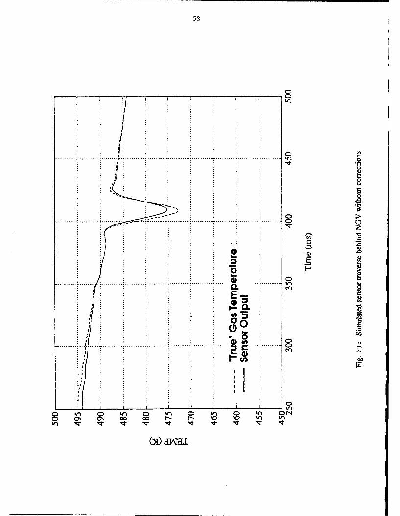
temperature difference) but inadequate for aerodynamic performance determination. An additional
transient error source is introduced when a probe is travers.-.-I through thermal gradients such as
wakes. This effect was simulated by driving a time accurate conduction model of the temperature
probe with the output of a 2-D viscous multi-blade row calculation of the flow in the turbine (Fig.
23). A measured blowdown tunnel transient is shown in the temperature time history of Fig. 24,
in which the top trace (labeled "gas") is the output of the micro disk thermocouple. A second
thermocouple was mounted at the bottom of the 75 pm diameter quartz stem (labeled "stem
bottom"). The gas trace illustrates the rapid temperature rise as the tunnel starts at 80 ms and the
slow decay as the supply tank blows down. The stem bottom trace reflects the temperature rise of
probe support structure, which is non-negligible over the first 500 ms of interest. The differences
between the two traces is a measure of the driving temperature difference responsible for the
transient conduction error. Given measurement of this temperature difference, the conduction
error can be estimated and a correction made. The accuracy to which this procedure can be
implemented must be established by calibration and will be discussed in a later section. The
principal disadvantage of this approach is that twice as many sensors, signal conditioners, and data
recording channels are required compared to just single thermocouple measurements.

20 J
5.1.1 Inletak!
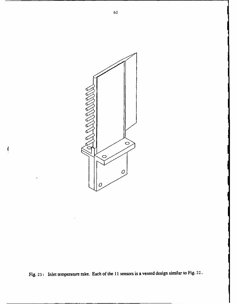
The inlet rake consists of 11 Kiel head measurement points (2 sensors each) arranged to
sample equal areas in the 10 cm high annulus (Fig. 25). The unit is mounted on the inlet
circumferential translator, angled to account for the probe rotation velocity. Thermocouple (Type
K) wires are derotated by a coil and brought out through the pressure vessel wall. A "cold"
junction connection to copper leads is then made in a dewar. Rather than keep the dewar at the ice
point, the cold block temperature is measured with two 4-wire platinum resistance thermometer
devices (RTD's).
5.1.2 Turbine Exit Rake
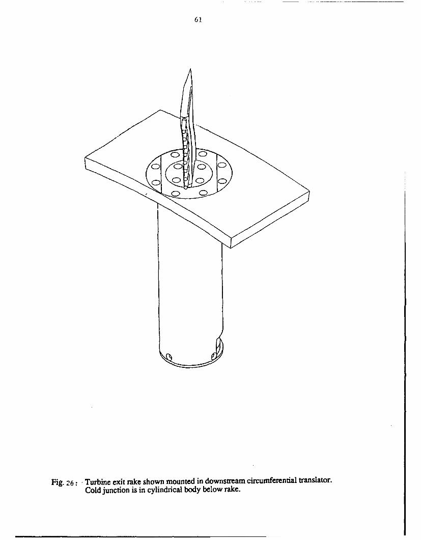
The turbine exit rake consists of 8 Kiel head measurement points (2 sensors each) arranged
to sample equal areas in the 3.7 cm high annulus (Fig. 26). The unit mounts to the turbine exit
circumferential translator, which presented two severe design constraints. The first is that the rake
must be readily removable from the blowdown tunnel with the rotor in place for calibration. The
only access is through the three small instrumentation ports. This suggested placing the cold
junction within the probe body itself so that all thermocouple wires and joints are included in the
calibrations. The second constraint is space, since the turbine exit translator is retrofit to an area in
which no provision had been made during the initial facility design. The final probe design houses
a copper cold plate in a cylindrical housing below the flow path. The thermocouple wires
transition to copper on solder pads on the cold plate. The cold plate temperature is monitored by
two RTD's. There is sufficient thermocouple wire within the rake body to permit separation of the
rake head and cold plate for calibration. The bottom of the rake assembly is a 41 pin electrical
connector so that the entire unit simply plugs into the exit translator.
5.13 Temperature Rake Signal Conditioning
Each of the rake sensors (11 upstream, 8 downstream) has two thermocouples and thus
requires two signal conditioners and two A/D channels. The principal requirements for the
conditioners are low noise (compared to the thermocouple output) and long-term stability (since
the amplifiers must remain stable between calibrations, hopefully several weeks). Analog devices

21
2B31H instrumentation signal conditioners were selected. They are operated at a gain of
approximately 800 and the internal two pole filters are set at 500 Hz. The same units are also used
as RTD signal conditioners for the cold junction references. Forty-two channels have been built.
The data acquisition system has been expanded with the addition of an Analogic 64-
channel, 16-bit, PC-based A/D subsystem. The maximum aggregate sampling rate for the unit is
200 kHz. Software has been written so that this unit mimics the functionality of the existing
blowdown turbine data system (41 channels at 200 kHz per channel plus 128 channels at 16 kHz
may rate per channel). The new unit is required because of inadequate stability for aero
performance of the older low speed channels as well as lack of capacity.
5.1.4 Temperature Rake Calibration
Three calibration steps are required to establish the rake accuracy. The first is a steady state
voltage output versus temperature calibration. This will be performed in a stirred silicon oil bath
over the 300-500*K range of interest. A secondary standard (0.01*K) platinum RTD is the
temperature reference. The second step is to establish the long-term stability of the sensors, signal
conditioners, and A/D, which will be established by multiple calibrations. The third and final step
is determining the overall accuracy of the rake in measuring gas temperature, which will include
the transient conduction and recovery factor corrections.
The final aerodynamic calibration of the rakes requires that: (a) the freestream temperature
be uniform and known to the necessary accuracy (0. 1-0.3*K); (b) the freestream Mach number be
variable to match the turbine inlet and exit conditions; and (c) the flow turn on with approximately
the same time constant as the blowdown tunnel (30-50 ms). To accomplish this, we have built a
75 mm diameter blowdown test tunnel using blowdown turbine components (Fig. 27). The
heated gas supply is the blowdown turbine supply tank (-11 m3 volume). The flow is turned on
and off using the 75 mm diameter, fast-acting (15 ms) coolant supply valve. An orifice at the test
section discharge is used to establish the Mach number. The test tunnel is closely coupled to the
supply tank to keep the thermal boundary layers thin at the probe location. The supply tank gas is
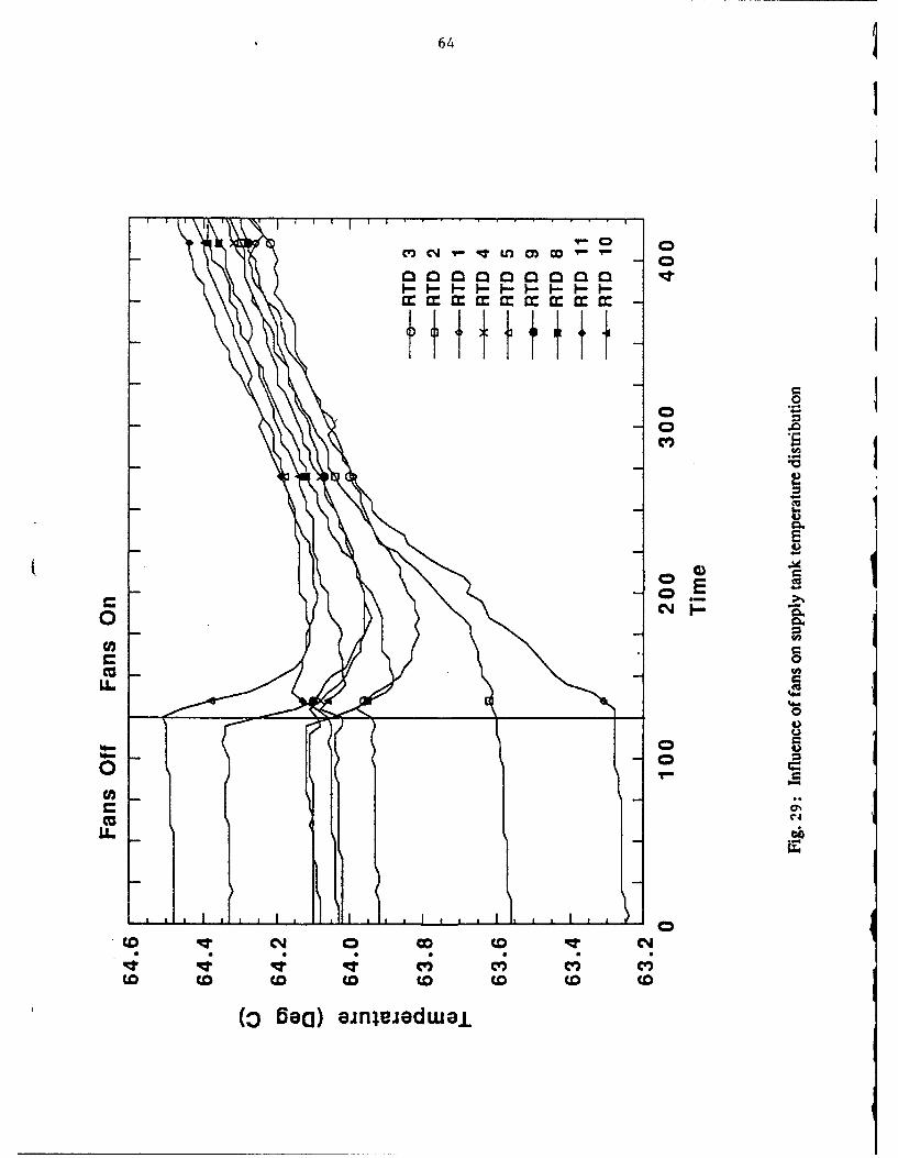
homogenized prior to the test by three fans. The temperature distribution is established by 11
22
platinum RTD's spotted through the tank (Fig. 28). The RTD's are bath-calibrated against a
secondary standard before installation. Figure 29 is data taken from the tank sensors and shows
that the temperature is uniform to about 0.2)K.
The tank RTD's and fans have been removed from the supply tank for the turbine testing.
The plan is to bath calibrate the temperature rakes, run the turbine tests, and then, in the late
summer-early fall time frame, set up the test tunnel and run the calibration checks.
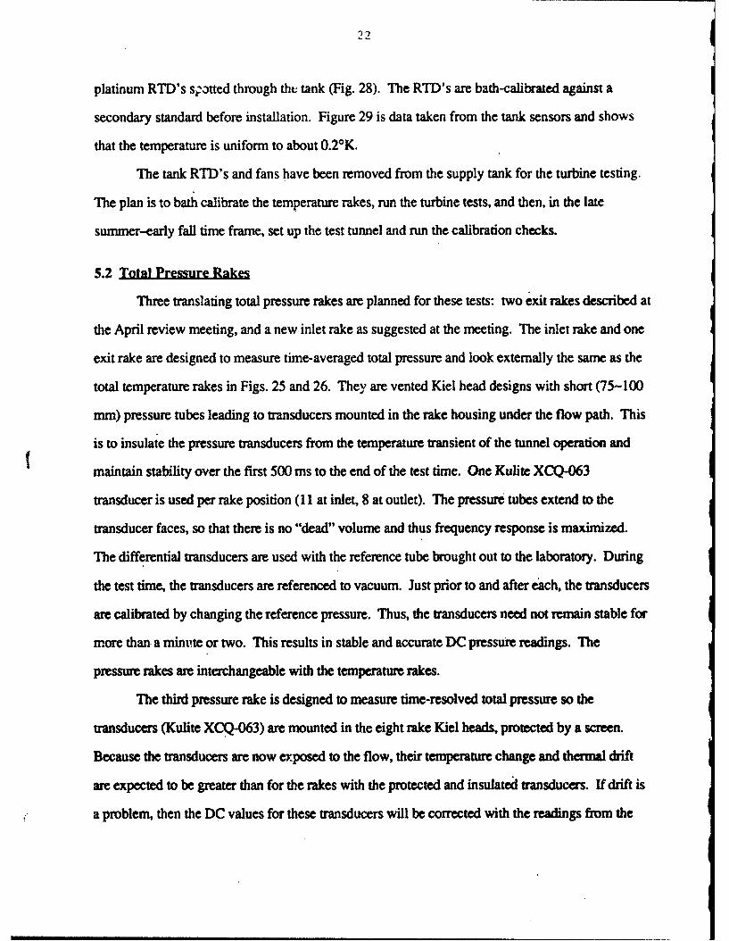
5.2 Total Pressure Rakes
Three translating total pressure rakes are planned for these tests: two exit rakes described at
the April review meeting, and a new inlet rake as suggested at the meeting. The inlet rake and one
exit rake are designed to measure time-averaged total pressure and look externally the same as the
total temperature rakes in Figs. 25 and 26. They are vented Kiel head designs with short (75-100
mm) pressure tubes leading to transducers mounted in the rake housing under the flow path. This
is to insulate the pressure transducers from the temperature transient of the tunnel operation and
maintain stability over the first 500 ms to the end of the test time. One Kulite XCQ-063
transducer is used per rake position (11 at inlet, 8 at outlet). The pressure tubes extend to the
transducer faces, so that there is no "dead" volume and thus frequency response is maximized.
The differential transducers are used with the reference tube brought out to the laboratory. During
the test time, the transducers are referenced to vacuum. Just prior to and after each, the transducers
are calibrated by changing the reference pressure. Thus, the transducers need not remain stable for
more than a minu'te or two. This results in stable and accurate DC pressure readings. The
pressure rakes are interchangeable with the temperature rakes.
The third pressure rake is designed to measure time-resolved total pressure so the
transducers (Kulite XCQ-063) are mounted in the eight rake Kiel heads, protected by a screen.
Because the transducers are now exposed to the flow, their temperature change and thermal drift
are expected to be greater than for the rakes with the protected and insulatedl transducers. If drift is
a problem, then the DC values for these transducers will be corrected with the readings from the

23
steady-state rake.
5.3 Static Pressure Taos
Wall static pressure taps have been added to the inner and outer annulus walls at the NGV
trailing edge (mid-passage), and at the inner annulus at the turbine exit translator at the rake axial
station. All three consist of short tubes (50-100 mm) fed through Kulite XCQ-093 transducers.
6.0 Rotor Blade Heat Flux Instrumentation
Since a principal output of this research program is a set of detailed rotor blade heat transfer
measurements, the rotor blade instrumentation is the single most important part of the facility
preparation. It is also the most time consuming and expensive by far, with more than one half the
program resources to date being expended in this area. For this program, the instrumentation has
been entirely redone, including the manufacture of transducers, their mounting and wiring, and
blade calibration.
Three blades have been produced, each instrumented about their chord with the spanwise
location differing among blades. A composite of the three blades is shown in Fig. 30, which
illustr.tes the heat flux gauges' locations. Thirty-nine gauges are fully functioning. An additional
five have just the top sensor operational, in which case essentially all information can be retrieved
with some additional data reduction effort On three additional sensors, only the bottom sensors
are working, in which case little information can be extracted. Two additional gauges are mounted
on the blade platform near midpassage at the leading edge plane. Resistance thermometers are
mounted to the underside of the blade platforms to serve as pre- and post-test temperature
references which facilitate scale factor and drift determination.
The wiring for each of the three blades is shown schematically in Fig. 31. The signals
from each transducer is brought out by slip rings. The signals are then fed through 34 bridge
amplifiers (DC-50 kHz bandwidth) and into individual data acquisition channels (200 kHz
sampling rate for the top sensors, 16 kHz for the bottom sensors).
The blades have been completed and the 94 amplifiers required checked out. Blade

24
calibration will be done as the NGV-only testing is ongoing in order to free up manpower for
readying the facility.
7.0 £ED Mctmivi
The principal CFD tool to be used at MIT on this program is the three-dimensional,
unsteady, multi-blade row Euler code written by Saxer and Giles, UNSFLO3. This is an explicit
time-marching, node-based, Ni-Lax-Wendroff algorithm implemented on an unstructured grid.
Non-reflecting boundary conditions are applied at the inlet and outlet and at the stator-rotor
interface.
This code had been run on the experiment's NGV and rotor blade geometries by Saxer but
at equal NGV-rotor pitches rather than the 36 NGV's, 61 rotor blades of the rig. The grid
geometry has been modified to calculate 3 NGV passages and 5 rotor passages (i.e., 36 NOV, 60
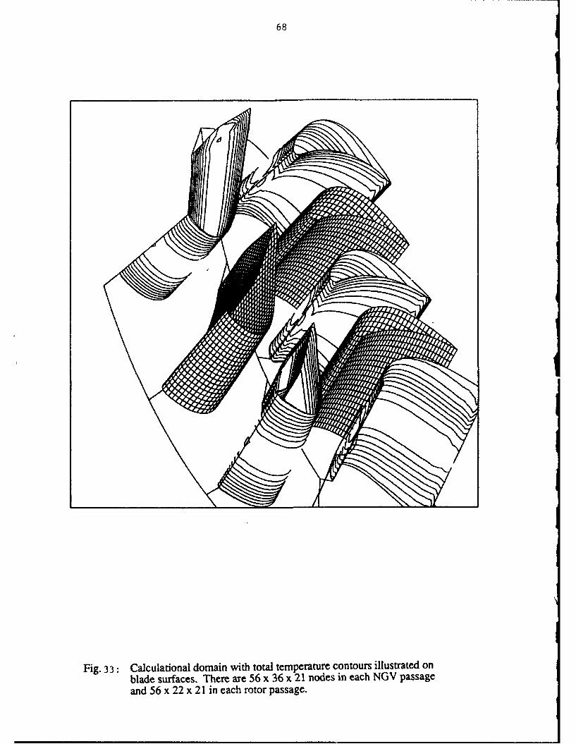
rotor blade count) as illustrated in Fig. 32. This grid is currently set up with about 256,000 node
points (56 x 36 x 21 in each of 3 NGV passages and 56 x 22 x 21 in each of 5 rotor passages). A
coarser version of the grid (only 9 rather than 21 radial planes) has been run to convergence as an
initial checkout. Rotor blade temperature contours are shown in Fig. 33. The finer grid is
currently running.
The inlet boundary conditions have been set up so that quite general radial temperature and
pressure distortions can be specified. Periodicity, however, constrains hot spot placement to one
every 3 NOV pitches where the experiment is set up as one hot spot for every 2 NGV pitches
(Fig. 34). After we gain some experience with the code, the blade count can be enlarged to 6
NOV's and 10 rotor blades to permit the experiment's periodicity to be modelled. This is at the
expense of doubling the run time, of course. The grids have been interfaced to the MIT 3-D
visualization codes.
In addition to UNSFLO3, the two-dimensional Euler version and a 2-D thin shear layer
viscous version are available at MIT and have been checked out with the experimental geometry.
Also available is John Denton's MULTISTAGE 3-D, steady, multi-blade row, Euler code.

25
Discussions are ongoing with NASA Lewis Research Center about using John Adamczyk's 3-D
viscous code.
8.0 Rig Prearatimns
Rig preparations included completion and installation of the new rake translators
refurbishment and repair of tunnel subsystems, installation and programming of new data
acquisition equipment, and instrumentation calibrations and cables. The inlet and outlet rake
translators were completed and installed in the rig. The units performed as designed during
vacuum testing.
Several of the rig subsystems required refurbishment and repair, which was not surprising
considering that the rig is 10 years old and had not been operated for about 3 years. The Freon
boiler in the gas mixing system failed pressure testing and was replaced as were numerous leaking
valves. The vacuum system valves and vacuum pumps were overhauled. When the test section
was disassembled to mount the rotor exit translator, it was discovered that a wire on one of the
eddy brake magnet coils was broken. This explains the sudden shift in brake calibration noted
during the previous test series. The eddy brake was removed for repair and will be re-installed
with the rotor.
8.1 Data Aaisition
Two new data acquisition systems have been added to supplement the current unit and
serve as backup (the current system is 11 years old). Sixty-four low speed channels have been
added. These units have 16-bit resolution (about 14 of which are usable given the noise levels at
the rig), and 3 kHz per channel maximum data rate. The unit is mounted in a '486 PC- These low
noise, high resolution channels have been allocated primarily to the temperature rake outputs.
Additional high bandwidth channels have been added as well. Thirty-two channel (24 arrived, 8
on order), 12-bit, 330 kHz per channel A/D's have been added in a second '486 PC. This unit was
purchased by the laboratory and will be shared with other experiments. This brings the total
channel capacity of the blowdown turbine facility to approximately 68 high speed analog channels

26
(200+ kHz per channel) and 192 low speed analog channels (3+ kHz per channel).
Both the new low and high speed data acquisition systems (A/D's plus computers)
required considerable custom cabling and programming. The units were programmed to interface
to the current data handling systems and are mostly transparent to the user.
8.2 Instrumentation Calibration
Upon completion of the A/D systems, the temperature and pressure rakes were DC
calibrated. The temperature rakes are of a pitot-type configuration with two type K thermocouples
at e,.h head position, one to measure gas temperature, the other to measure the temperature of the
new stem on which the first is mounted, to permit corrections for conduction errors. The rakes are
designed with local reference hot junctions rather than standard remote cold junctions (Fig. 35a).
This arrangement facilitates rapid recalibration of the rakes without necessitating teardown of the
test section, as would be the case if thermocouple leads were run out to exiernal cold junctions.
(The rakes can be removed through windows in the test section while leaving the cabling in place.)
The hot junctions consists of an insulated copper block on which the thermocouple to copper wire
connections are made. The block is instrumented with two resistance thermometers (RTD's).
Calibration consisted then of two steps - calibration of the reference junction sensors followed by
calibration of the thermocouples. Both were done in a stirred bath of silicon oil against a
secondary standard platinum RTD stable to 0.0I*C. The calibrations were performed through the
entire data chain - sensor, cabling, signal conditioners, data acquisition system. Transducers
agreed with each other to 0.1*C. Repeatability of calibration was within 0.20 C.
The pressure transducers in the rakes (Fig. 35b) are readily calibrated since each is a differ-
ential transducer with a reference pressure which is brought out of the rake and through the transla-
tor. In practice, the transducers are calibrated in place immediately before and after each test. The
pressure transducers were checked for temperature sensitivity by calibrating them in an oven at
temperatures up to 1OO'C. All transducers are stable to better than 1% over the temperature range.

27
8.3 Instrumentation Performance on Translators
The rake instrumentation was installed in the translators (Fig. 35c) which were then run in
vacuum as an operational check. The pressure rakes' operation was satisfactory in that no
extraneous signal or noise was observed on the pressure transducer outputs during the translator
motion (Fig. 6). The temperature outputs, however, did show artifacts due to both translator
motion and operation of the DC servo systems driving the two translators. A signal related to the
motion can be seen on the output from an inlet rake thermocouple in Fig. 36, starting at about 200
msec (same time scale as in Fig. 6). The signal is similar in shape and magnitude on all 22
thermocouples on the inlet rake. The signals are clearly related to the probe motion in that they do
not appear on the reference RTD signals (Fig. 37) which are mounted in the stationary frame for
the inlet rake. The magnitude of this unwanted signal, about O.20C, is sufficiently low that it does
not serve as a hindrance to this research program but, at this level, it is a major component of the
upstream gas temperature measurement uncertainty.
The level of unwanted signal is much greater on the outlet temperature rake, as can be seen
in Fig. 38, in which the 'noise' amplitude is about 30C. As with the inlet rake, the signal is similar
on all the thermocouples on the rake to a remarkable degree (Fig. 39). Unlike the inlet rake,
however, the outlet temperature reference RTD's are on the rotating system and these exhibit a
signal amplitude similar to that of the thermocouples, Fig. 40. (The plotted 'reduced'
thermocouple temperature traces incorporate the RTD signals since these are reference sources
which are differenced with the raw thermocouple temperature.)
The level of temperature uncertainty represented by the level of interfering signal on the
outlet temperature rake (30C) is clearly unacceptable for aeroperformance measurements and
marginal for reducing heat transfer measurements. Therefore, considerable effort was put into
understanding this problem. Sources of the interference considered included some combination of
magnetic pickup on the rotating system, cross-talk between layers of cabling, grounding problems,
etc. The presence of this signal on the outlet RTD's (which were operated in a 4-wire
configuration to eliminate common signals induced in the leads) and its absence on the pressure
rakes (4-wire bridge configuration) which share the same cabling was particularly puzzling.
Comparison of these signals, as in Fig. 41, was interesting but unenlightening. Circuit modelling
and bench testing were unsuccessful in reproducing or explaining the problem. Mu metal
shielding was added to the cabling to exclude magnetic fields with no avail. Finally, the grounding
scheme of the rakes was modified in an ad hoc manner. This succeeded in reducing the induced
signal on the exit rake by more than an order of magnitude (Figs. 42 and 43), to less than 0. 150 C.
Only minor improvement was observed in the upstream rake output (Fig. 44). At its current level,
these unwanted signals will not adversely affect the current research program. We fixed things
without understanding why and will now retire from the field of battle clothed in graceful victory
and ignorance.
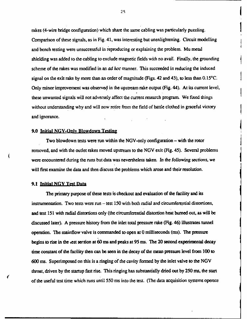
9.0 Initial NGV-Only Blowdown Testing
Two blowdown tests were run within the NGV-only configuration - with the rotor
removed, and with the outlet rakes moved upstream to the NGV exit (Fig. 45). Several problems
were encountered during the runs but data was nevertheless taken. In the following sections, we
will first examine the data and then discuss the problems which arose and their resolution.
9.1 Initial NGV Test Data
The primary purpose of these tests is checkout and evaluation of the facility and its
instrumentation. Two tests were run - test 150 with both radial and circumferential distortions,
and test 151 with radial distortions only (the circumferential distortion heat burned out, as will be
discussed later). A pressure history from the inlet total pressure rake (Fig. 46) illustrates tunnel
operation. The mainflow valve is commanded to open at 0 milliseconds (ms). The pressure
begins to rise in the test section at 60 ms and peaks at 95 ms. The 20 second experimental decay
time constant of the facility then can be seen in the decay of the mean pressure level from 100 to
600 ms. Superimposed on this is a ringing of the cavity formed by the inlet valve to the NGV
throat, driven by the startup fast rise. This ringing has substantially dried out by 250 ms, the start
of the useful test time which runs until 550 ms into the test. (The data acquisition systems operate
29
at their highest rate, 200 kHz per channel, during this 250 to 550 test time.) This time trace also
illustrates the radial flow uniformity at the tunnel inlet and thermal drift limits of the transducer.
All six of the radial stations agree to within one percent, and five of the six to 0.5%. We believe
that the sixth transducer's performance can be improved with additional calibration.
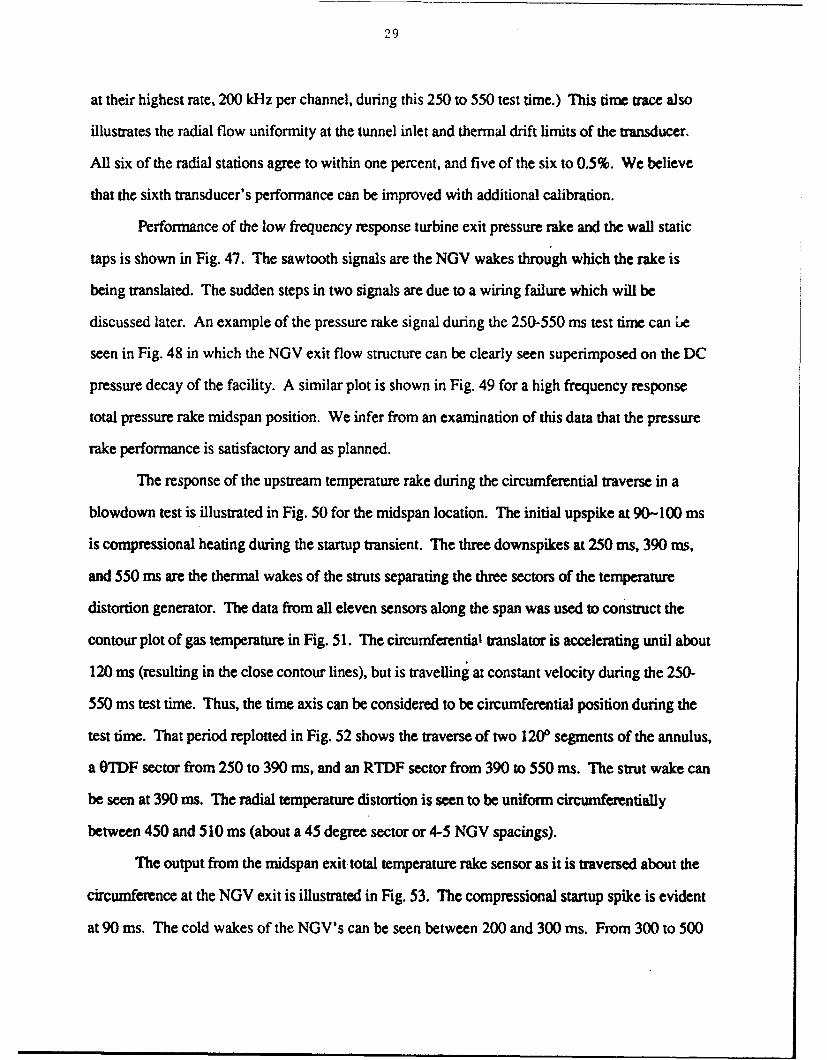
Performance of the low frequency response turbine exit pressure rake and the wall static
taps is shown in Fig. 47. The sawtooth signals are the NGV wakes through which the rake is
being translated. The sudden steps in two signals are due to a wiring failure which will be
discussed later. An example of the pressure rake signal during the 250-550 ms test time can le
seen in Fig. 48 in which the NGV exit flow structure can be clearly seen superimposed on the DC
pressure decay of the facility. A similar plot is shown in Fig. 49 for a high frequency response
total pressure rake midspan position. We infer from an examination of this data that the pressure
rake performance is satisfactory and as planned.
The response of the upstream temperature rake during the circumferential traverse in a
blowdown test is illustrated in Fig. 50 for the midspan location. The initial upspike at 90-100 ms
is compressional heating during the startup transient. The three downspikes at 250 ms, 390 ms,
and 550 ms are the thermal wakes of the struts separating the three sectors of the temperature
distortion generator. The data from all eleven sensors along the span was used to construct the
contour plot of gas temperature in Fig. 51. The circumferential translator is accelerating until about
120 ms (resulting in the close contour lines), but is travelling at constant velocity during the 250-
550 ms test time. Thus, the time axis can be considered to be circumferential position during the
test time. That period replotted in Fig. 52 shows the traverse of two 1200 segments of the annulus,
a OTDF sector from 250 to 390 ms, and an RTDF sector from 390 to 550 ms. The strut wake can
be seen at 390 ms. The radial temperature distortion is seen to be uniform circumnferentially
between 450 and 510 ms (about a 45 degree sector or 4-5 NGV spacings).
The output from the midspan exit total temperature rake sensor as it is traversed about the
circumference at the NGV exit is illustrated in Fig. 53. The compressional startup spike is evident
at 90 ms. The cold wakes of the NGV's can be seen between 200 and 300 ms. From 300 to 500

30
ms, the rake is traversing through the OTDF sector, whose heater was burned out during this test,
so that the temperature is quite low. After examining the temperature data, we conclude that the
temperature instrumentation is operating as designed and that its performance is satisfactory for
this research project.
9.2 Exit Rake Translator Wiring Problems
During the first NGV-only blowdown tests, the wiring which runs from the translator to
the stationary frame was seriously damaged. The wiring consists of three 50-conductor ribbon
cables sandwiched between four layers of 75 pm stainless steel shim spring stock. The multi-
layer cable is 3/4 of a rnLter long and arranged in a hairpin with one end fastened to the rotating
translator and the other fixed to the stationary test section. The cable is located at the rear of the
turbine exit flow path in a protective shroud. This loop arrangement (Figs. 8 and 54) facilitates
360 degree travel during the test. The shims both protect the ribbon conductors and provide the
restoring force needed when the translator is reset between tests. Unfortunately, the ribbon blew
out under its containment shroud and became entangled in the chain drive (Fig. 55) approximately
250 ms into the first test.
Several solutions were considered, including a rotary seal on the protective shroud and
various modifications to the laminated ribbon assembly. The geometric constraints of the test
section proved very restricting. A full-scale mockup was constructed to evaluate various schemes.
The approach adopted was (a) to stiffen up the ribbon assembly by replacing the outer two 75 pm
thick shims with 150 lim shims, and (b) the addition of a rotating containment ring at the inner
radius of the stationary protective shroud. This ring increases the moment of inertia of the rotating
system, slowing the translator acceleration.
10.0 Temperature Distortion Generator
The temperature distortion generator used for these tests is the honeycomb storage matrix
unit originally designed for RTDF tests. It uses electric heating wires at midspan as a heat source
and oil cooling jackets on the inner and outer flow path walls to serve as heat sinks, thus generating
31
a parabolic temperature profile across the annulus during the pretest heatup period. The unit was
modified for OTDF testing by spacing the heating wires along the circumference in one 120"
sector to generate hot spots, one hot spot per two NGV pitches (Fig. 1).
Previous testing had shown that the generator was contaminated with fine particles during
manufacturing which destroyed the rotor blade heat flux instrumentation. Therefore, a 1000 liter
ultrasonic cleaner was constructed so that the generator could be immersion cleaned. After each
cleaning, the water was drained and filtered and the particles counted. The cleaning was repeated
until no particles could be discerned.
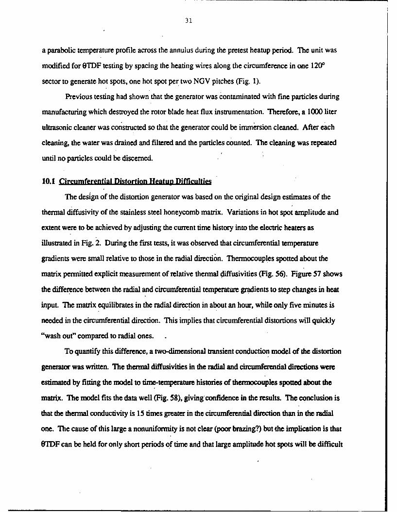
10.1 Circumferential Distortion Heatun Difficulties
The design of the distortion generator was based on the original design estimates of the
thermal diffusivity of the stainless steel honeycomb matrix. Variations in hot spot amplitude and
extent were to be achieved by adjusting the current time history into the electric heaters as
illustrated in Fig. 2. During the first tests, it was observed that circumferential temperature
gradients were small relative to those in the radial direction. Thermocouples spotted about the
matrix permitted explicit measurement of relative thermal diffusivities (Fig. 56). Figure 57 shows
the difference between the radial and circumferential temperature gradients to step changes in heat
input. The matrix equilibrates in the radial direction in about an hour, while only five minutes is
needed in the circumferential direction. This implies that circumferential distortions will quickly
"wash out" compared to radial ones.
To quantify this difference, a two-dimensional transient conduction model of the distortion
generator was written. The thermal diffusivities in the radial and circumferential directions were
estimated by fitting the model to time-temperature histories of thermocouples spotted about the
matrix. The model fits the data well (Fig. 58), giving confidence in the results. The conclusion is
that the thermal conductivity is 15 times greater in the circumferential direction than in the radial
one. The cause of this large a nonuniformity is not clear (poor brazing?) but ihe implication is that
OTDF can be held for only short periods of time and that large amplitude hot spots will be difficult

32
to achieve. This is illustrated in Fig. 59, which shows the result of a transient heat calculation of a
sector with two hot spots. At heater current levels compatible with past practice, a 60 to 800 C hot
spot is achieved in two minutes. After an additional two hours of heating, these relatively small
hot spots are now superiinposed on a large radial temperature profile. This pattern is quite similar
to that in an engine (good) but not so convenient as pure OTDF for simple analysis (bad).
One solution to this problem is very fast, high current spikes applied immediately (1-3
minutes) before the start of a test. The constraint is the current level which can be put into the
heater before mechanical failure (burnout) of either the heater wire or its termination. This was
investigated experimentally on a test rig in vacuum, and it appears that OTDF's of 20% can be
generated before either the heater wire burns out or the brazed matrix is damaged.
The solution adopted was to double the number of heater wires at each spot from 2 to 4,
thus doubling the heat input. The OTDF wires are operated at currents of 30 amps (as opposed to
10 amps in the RTDF sector), increasing the heating rate by nine times. This high heat rate is
applied five minutes immediately prior to the blowdown test and should produce hot spots of
approximately 50*C. Vacuum tests with thermocouples in the matrix indicated this to be a viable
approach. As of this time, one half pressure test has been run at low current (20 amps) as a
mechanical checkout. Its results are inconclusive insofar as 0TDF levels achievable.
10.2 Distortion Generator Contamination
Although the generator was thoroughly cleaned before testing, aluminum witness cylinders
were placed in the flow path at the NGV exit. Microscopic examination after the first test showed
significant impact, equivalent to about 105 particles per test if the sampled area is extrapolated over
the entire flow annulus. This level of contamination is unacceptable.
Particles were collected and examined. Two types were noted - clear spheres of about 50-
100 pm diametr, and brown cubes of similar size. Since clear spheres did not dissolve in any
acid other than hydrofluoric, they are thought to be glass sandblast beads. The brown particles did
not dissolve in any acid. They closely resemble and are thought to be aluminum oxide abrasive
33
particles, also used for sandblasting.
The question is, of course, how to remove the particles. The ultrasonic cleaning removed
all the particles that ultrasonic cleaning will remove. What to do about the rest? Mechanical
cleaning techniques considered included shaking the unit on a 100 g shaker used for satellite
prelaunch testing, repeated heating and blowing cycles, and steam cleaning. Chemical means of
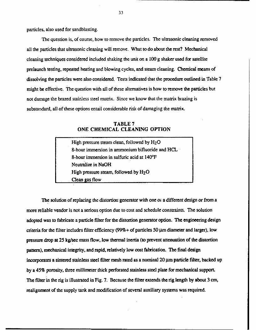
dissolving the particles were also considered. Tests indicated that the procedure outlined in Table 7
might be effective. The question with all of these alternatives is how to remove the particles but
not damage the brazed stainless steel matrix. Since we know that the matrix biazing is
substandard, all of these options entail considerable risk of damaging the matrix.
TABLE 7ONE CHEMICAL CLEANING OPTION
High pressure steam clean, followed by H20
8-hour immersion in ammonium bifluoride and HCL8-hour immersion in sulfuric acid at 140OFNeutralize in NaOHHigh pressure steam, followed by H20
Clean gas flow
The solution of replacing the distortion generator with one oi a different design or from a
more reliable vendor is not a serious option due to cost and schedule constraints. The solution
adopted was to fabricate a particle filter for the distortion generator option. The engineering design
criteria for the filter includes filter efficiency (99%+ of particles 50 prm diameter and larger), low
pressure drop at 25 kg/sec mass flow, low thermal inertia (to prevent attenuation of the distortion
pattern), mechanical integrity, and rapid, relatively low cost fabrication. The final design
incorporates a sintered stainless steel filter mesh rated as a nominal 20 gtm particle filter, backed up
by a 45% porosity, three millimeter thick perforated stainless steel plate for mechanical support.
The filter in the rig is illustrated in Fig. 7. Because the filter extends the rig length by about 3 cm,
realignment of the supply tank and modification of several auxiliary systems was required.

3
At this time, one blowdown test has been run at one-half pressure with the filter in place.
No mechanical problems were encountered. The trapping of particulates was evident when the
filter was disassembled for inspection after the test. Thus, this problem appears solved.
11.0 Gas Availability and Test Costs
Since the blowdown turbine facility was last operated, the cost of Freon-12 has risen
tenfold, from $1/lb to $10/lb. With allowance for leakage and aborted tests, this translates to
$1200 per test for Freon, a cost level which is not in the current budget. There are several possible
alternative approaches to this problem, including:
a) Running fewer tests
b) Testing with the Freon- 12 replacement, HC- 1 34a
c) Recycling the gas mixture
d) Testing in air at y = 1.4
e) Testing with an argon and C02 mixture at the proper y
f) Some combination of the above.
Each of these approaches has some advantages and serious disadvantages which are discussed
below.
(a) Obviously, running fewer tests is the most unattractive since the entire point of the
project is to take data; the data, however, must be relevant, i.e. properly scaled conditions.
(b) The Freon-12 replacement,.Hc-134a, is 20% more expensive so it does not represent a
useful alternative.
(c) Recycling the gas mixture is technically feasible but somewhat complicated since the
gas mixture is used at a pressure above that for condensation of Freon- 12 at room temperature.
Also, a relatively large amount of gas (20-50 kg) is used. Initial estimates are that such a
recycling system would cost between $50,000 and $100,000 and take 4-6 months to get working.
Thus, this solution is not compatible with the current project budget and schedule.
(d) Running tests in air is inexpensive but requires a 25% increase in rotor speed to

35
maintain constant corrected speed. This represents a 50% increase in rotor (no problem) and
instrumentation (may be a problem) stress levels. This speed increase is in addition to the 20%
increase over the original tunnel design speed needed to operate at the -10P rotor incidence angle
that is now the standard operating.condition. This places the rotor speed at 8,000+ RPM, very near
the dyna'mic limit of the current rotating system. Also, of course, yis 1.4 rather than 1.28.
(e) Gas mixtures other than argon-Freon have been considered. One of the most benign is
argon and C02 mixed to the proper yof 1.28. 71 's has a molecular weight of 42 and a speed of
sound 114% of that of argon and Freon. Thus, it represents a low cost alternative with a less
extreme increase in rotor speed and stress levels.
None of these options are all that attractive but we are-unaware of any other alternatives.
The current plan for the NGV-only testing is to (a) run most tests in air, (b) run a set with argon-
002 for comparison, and (c) run two Freon tests for reference and comparison with previous
running. For the rotor tests, the first few tests will be with the standard argon-Freon mixture. The
principal concern here is to avoid stressing of and damage to the rotor instrumentation until a
baseline set of tests have been completed (or the budget is exhausted). Testing will then switch to
argon-CO2.
12.0 Near-Term Plans
The plan for this winter is to conduct the NGV-only tests at the end of December and in
January. The rotor instrumentation will be calibrated in January and the rotor installed. The full-
stage testing should begin before February and continue through the spring.
13.0 Rfrences
1. Moss, R.W., and Oldfield, M.L.G., "Measurements of Hot Combustor Turbulence Spectra,"Rolls-Royce, plc, 1990.
2. Roach, P.E., "The Generation of Nearly Isotropic Turbulence by Means of Grids," Int. J. ofHeat and Fluid Flow, Vol. 8 (2), 1986.

36
U))
07Eci)
0 to
4.'

37
Co L
Cl)
0>
Low
0.LuC.
Co Co
'p _ _ _ _ _ _ _ _ _ _ _
- - - - - -n- - -dweS

38
IT , T7
CCow-
C)LU)z
co b

39
Servo MotorDrive
11 Station Rake
Distortion Test SectionGenerator c:: => Inlet Flow
Outlet Flow
Fig. 4: Inlet rake trnmslator
40
LI
CLC
0 hmo0
I.0
E
o >0II*
00UU
CLt

41
0.45
0.4-
0.35 -
0.3-
•'.0.25
"0 0.2-
L 0.15
0.1
0.05
0-
-0.050 .... 100 200 300 400 500 600
TWME: (ms)
350
300
250
*" 2000
P 150
50o'°C[
0
0 100 200 300 400 500 600
TIME: (ms)
Fig. 6: Measured performance of unstream rake translator

42
to1141111111
43
0
000
UU,
-e 0
44
InletRakePlane
I a.
I S I
I'
I
Boundary NGVLayer Bleed Leading Edge
Fig. 9: Alternate locations considered for turbulence grid placement

45
-------------
E ~,,A-/CL.
In C;£ (.
Ntm
- I
t)~rn ~ =-~

46
00
Ucc
*1*0 000
Cl)C 0
F-I -
Q: El

47
0r-
9
0.
000
'i
0N
LiL
48
30
~20-
8 Calibration I10o Calibration 2
volts
Figure 13: Hot wire calibration graphs

49
Figure 14: Turbulence grid dimensions

50
-35
-40
-45 - Theory (Roach, 1987
• -50 Re=1.5*IOM _-55
-60-
-65 Re=5* 10'A3
-70101 102 103 104
Wavenumber k(1/m)
Figure 15: Reynolds number effect

51
-35
-40 Measured
-45 - Theory (Roach, 1987)
-50
-55
-60-
-65
1102 103 104
Wavenumber k(1/m)
Figure 16: PSD; 1/2 NGV location

52
-35
-40 -
-45 MeasuredTheory (Roach, 1987)
"-50
•-55
--60
-65
-70101 102 103 104
Wavenumber k(1/m)
Figure 17: PSD; NGV location

53
-35
-40
-45 Theory (Moss and Oldfield, 1990)1
" -50 -
S-55 Measured~ 55-
-60-
-65 -
1 102 103 104
Wavenumber k(l/m)
Figure 18: PSD nozzle case NGV location

54
-40-
-45 Position 2
-5o
S-55 Position 1
-60-
"-65-
102 103 104
Wavenumber k(1/m)
Figure 19: Positioning effect parallel to nozzle

55
-35
-40
-45 2
S-50
-5 Position I "'-55
-60
-65
-1 102 103 104
Wavenumber k(1/m)
F 20: Positioning effect in direction of nozzle contraction

56
8
7-
6-
5-
0.0 0.2 0.4 016 0. 1.0
Inner Wall x/d Outer Wall
Figure 21: Turbulence intensity variation

57
0
04)
0-0
cm/
E4E
EEO: /
oII"
.0,
I.
G..w
ow
53
.. . .... . . . . . . .. . . . . . .. . . . . .. . . . .
............... ..... .. ........... . ....... ........ . ..... .~..
4)
JU
: ;I .: .. ........... .......
.......... .-- ...........
C V) in ON: :
0 coI r- ! ! . - " %-0"1t 't
S.........• ,l • ... •................................ :• • ';.........*• * :
! :/ i . -.
: ' ii i [0.i ! o
•' i i i I [
S! [ i

59
CD
_ _ II _ _
CD,
0.
ciin
C)
aV
0
(COj
oob 09 He 00
60
Fig. 25: Inlet temperature rake. Each of the 11 sensors is a vented design similar to Fig. 22.
61
Fig. 26: 'Turbine exit rake shown mounted in downstream circumferential translator.Cold junction is in cylindrical body below rake.

62
o. Z I 7777J
4)
V) 4. / )a-0 Da)= 0
CC
00
(0 >
4)

63
CA...
0..2
<., CM
LM2
toh
u-
64
I
0J
mo~omocooI- !- I- i- I-- I-- I-- !--
C00
0-
CI-
)U
we e
(o Be]) anjeje~ual

65
00
Q 0
*0 Emc
0 0~
16-
E~lE101111 1
LU r
0- o_ d
0-0m EnV* *
0 CMc:a c
cci
co r

(66
0
Iz
CL U)
cc.
ooo
Jt
0'
0 -m
U)U
0 U
[~~~jc 00 _
x
L'-I liei lii ii Cz

67
Fig. 32: 3 NGV, 5 rotor blade grid geometry illustrated for the hub plane
68
Fig. 33: Calculational domain with total temperature contours illustrated onblade surfaces. There are 56 x 36 x 21 nodes in each NGV passageand 56 x 22 x 21 in each rotor passage.

69
Temperature 3 Nozzle 5 RotorDistortion Passages Passages
Sx
Fig. 34; The circumferential period, X., of the inlet temperature distortion
must match the 3 NGV-5 rotor grid geometry

07
CuL
0,0
04,
E CD
a V,F.
*D 0
LOE
__ __ __ _ Z. bfA.Z
oo

4If
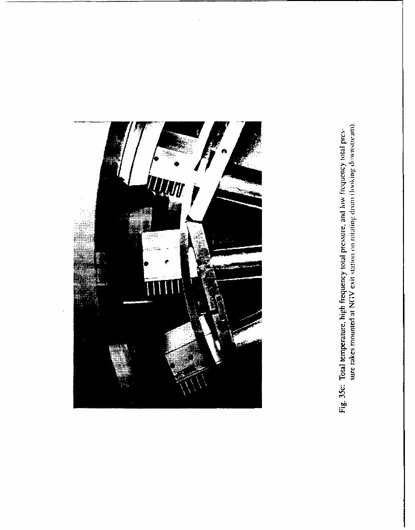
* 4-
'U
I- U- S.
C
U
U= -Ac=- C
- L.
o
U-1..
'U -I-
SES.
C)-C
4.)t�c-Cztie-
-C
U'- =
0-C)
In
a

73
.. . .. . . . . . . . . . . . . . . . . . . . . . . ... .. . . . . . .. . . . ... ... . . . . . . . . . . . .
* 00
.. . ... . . .. . . . . . . . . . . . .. . . . . .. . . ... . ... .. . .. .. .
.. . . .. . . . .. . . . . .. . . . . . . . . . . ..*. . . . . .. C )C
C).... .. .. .. .. .. .. .. ..... .. .. ... .. .. ..... ... .... ........ .. .... .... .... .. ..I. .. ....... .0.. .......... .................\0 Nr
C%4 N 14 C0
*oa~) a-fuy-mpui

74
...... __...__.... ......... ........
...........~~ .0 .......
Lp
.... ...... ......... ...... ... ............ ........
.. .... .. .... .... ... .... ..
.... ... .... ... .... ... ...... .... ... ....... ...
........... .......... ........ ............ ..........

75
............ ............................. • ............... :. . ......... ... ... . .............. ..............
...... ••........................ ....... ........
,.° .... . .......o....°°............................. ..
* °
-
ID-.S... ... ... ........... ..................... .............. ............. - .. . .............. ..-
S...... ........ .............................. •..... . ..... . .. .. .. .... ........ ........... . ...............
:.. .. .. ....
S.............. .............. 7............... ........ ... ...... ................. ..... . .C)U
S............. .................................. .. ..... ..... ...... .......... .............................. C14 4 U0
o 0I
........ ............. .............. ............... ... ......................... ..................... .
00
eri C,,4 N eq
N0

76
T 1 r i r I
_t I
•1 ---- iC)
. ..... .... .. , ...... .
._______._
• ................. •............. .... ......... . . .
...................... ............ ...........c-r-
S.............. . ......... .. .. .. .. .. .. .. .. .. .. .. .... ...... •
C)-
CD
......... .C
............ .... ...........
LLIo
No N 0
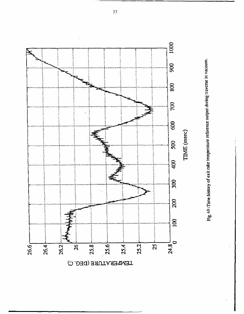
77
.. .. ... . . .. ... ........... . ...... . ......
00
.......... ......... . ......... ......... .......... .... ................. ...........-
......... ......... .... .................................
........... .....................
†...... ....... ...... ...... ...... ................... ............. ......... ................. ....... ........ ................ ...... 0
............~~ ~~~ ............................ . .................
0 UC4
......... ......... ......... ........
......... ....... ..... ................... ......... ................. .......
00 N 00
vi vi vi
0q Vq N
b~~ ~~ *Ea)aivdmA-

78
.. .. .. .......-... .. _ . . . . . . . . .
1 NO
.. ...... . . .. ..
I C)
I CIS
-. . . .. ...... ....
- .4: ~: -~ I.. . . . . . .. . . .... . . ... . . ..... .....
........... K - ~
SC))
... .. .. . .. .... . . . . . . .. .. ... .. .
. . .. . ........ . ..... . ..... ... ..... . ..
CC
.. .. .... .. -. Cse____*r
i.i

79
000
.. .. .. ... .. . .. .. .. . .. ... 0...
............ ........... ........... ........... ............. ..... C
... . . .. . . . ... .. . . ..... .. .
ý:0
bo
.. .. .. .. .. .. .. .. .. .. .. .. .. ... .. .. . ... .. .. .. .. .. .. .. . .. ..
(sniDTi4D) 2TwInvaa3JYu~

80
E
............... .. -... i...I.... .......... ,,. ......... . . . . . .. . . .
• Q
0 0.
.. ...... .. ...... .. ..
Soo
Sri \Cll v
N %n Ill In I4
ri N cC

. . . .. . . . . . . . . . . . . . .. . . .7 . . ... ... .. .
.l a
ui. 0I 0U..
OU
..... .... .. . .... ... .... .. . ...
_ _ _ . .. .. .. . .. . . .
............ .. . . .. .. . . . . .. . . . .
....... ;9 .... ........ ........... .....
cnU
.... ... ... ... .... .. ... .. .... ... .. ....
... .. .. . . .. .. .. . 7 .. .. ... ... .. . . .. .. ... .. . .. .. .. .. ... .. .. .. ... .. .. .U
00 \0 ~00 \0r
4 ~ CM CM
(SnIcr20o) aalmvuya~wl

.280
U) OR
E
I-b
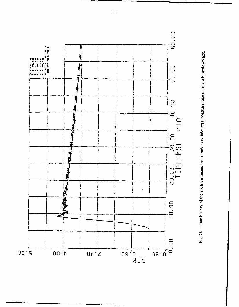
93
- - I
CDC
-0
-CD~
• E
.IP
LL.
O9 00 " b02o 0
ku-u
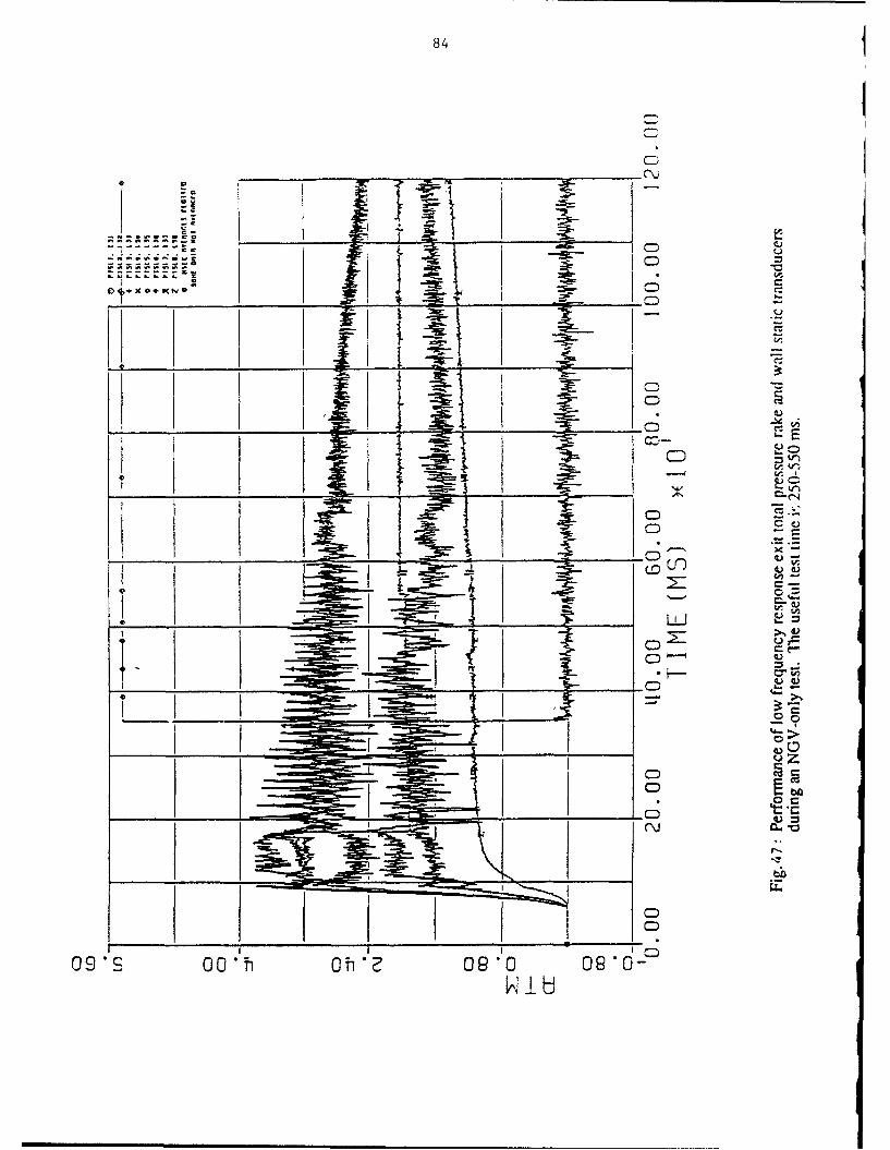
84 4
4t
-I• .-- 1•_____L
x~ ~jS- - . f•-•j o
C)_ _ _ I I .
0'D_ _ _ _ _ V
__ 1Z5-C
)-D 4
-Q V
9 0 ;hof '!090 080
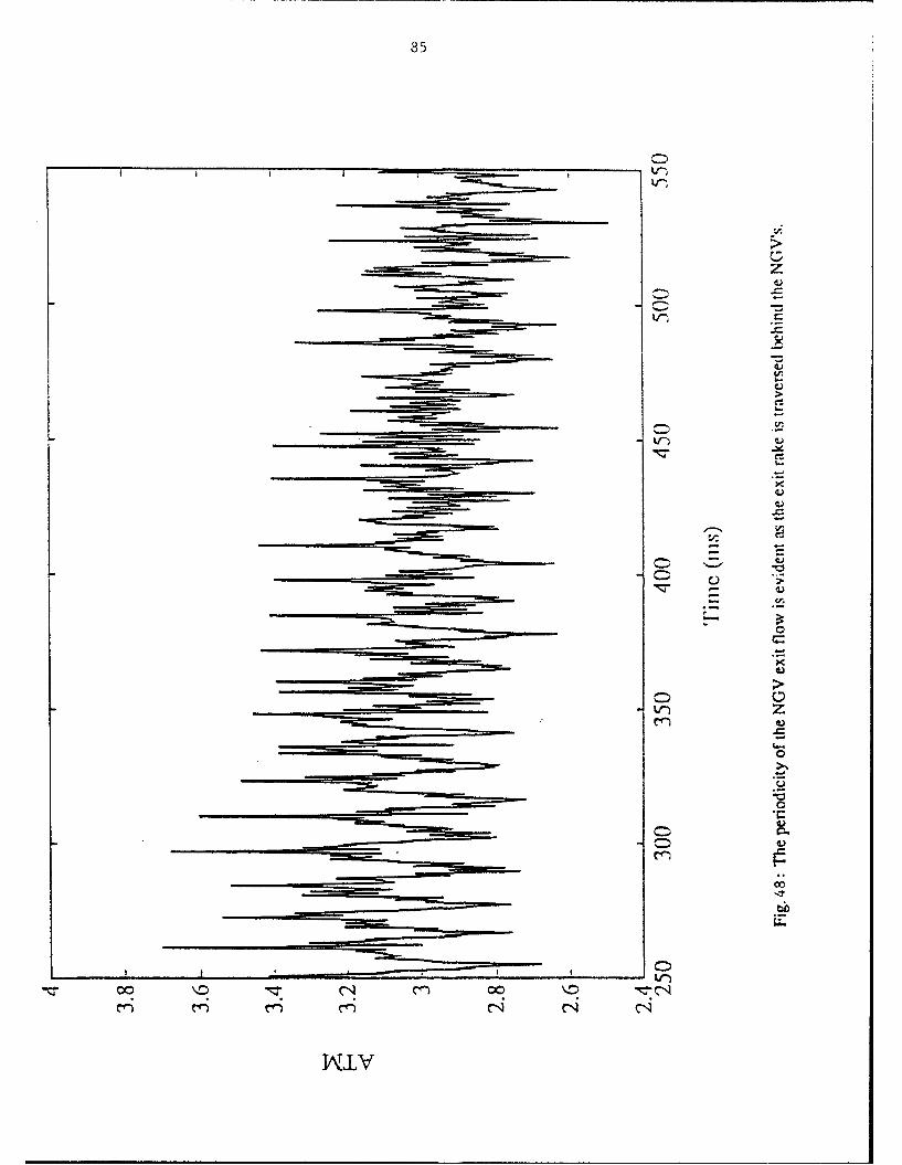
85
U-4)
CDC
L4r)
I I-
kr))
00 \.S
W, IV

86
t-v
>
C6
Ci
6-U'4 00 rrb 0
rC.)
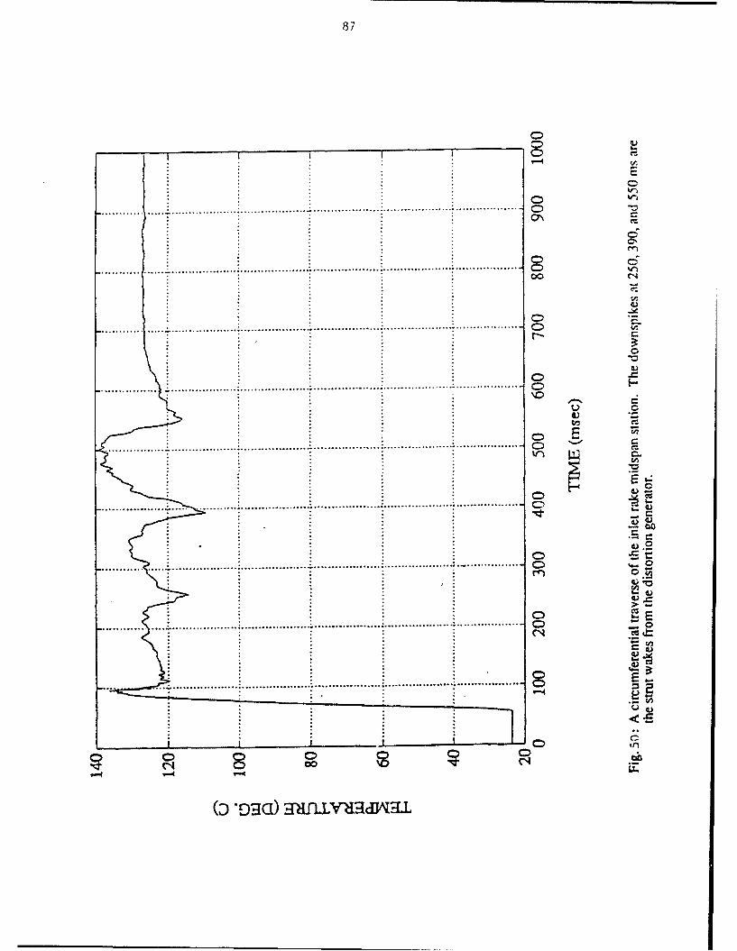
87
00
...... ..................................
00
........... ... ................................... 7 ......................................... 0
00
. ................................................................................ C
c6 c.
CA
C> C>
co C14
(D*Dg asfuv. Img.

. ... . .. . . . .. . ... ..
... . ... . . . ... ... .. . . ...
t A0
C5 00
(HolwNo~uocl Tqcr-

89
- C)
....... ... ........ ..... ...... ........ ........ ...................... .... ... .... ..... ...... ...... 0
0U 4).00.
\C-
00
060
WD-M) NOUS~c TV'CIV0

90
00
......... 7 .........
. . ... . . ... . . . . .. . . . . . .. . ... .. . . .. . . .. ... . .. . . . . .. . . . . . 0
.. . . . .. . . .. . . . . . . . .. . . . . .. . . . .. .. . . . .. . . ... ..... . . ... . . . .
z -
00 00 C 0
0,021a)~~ au-va-v-
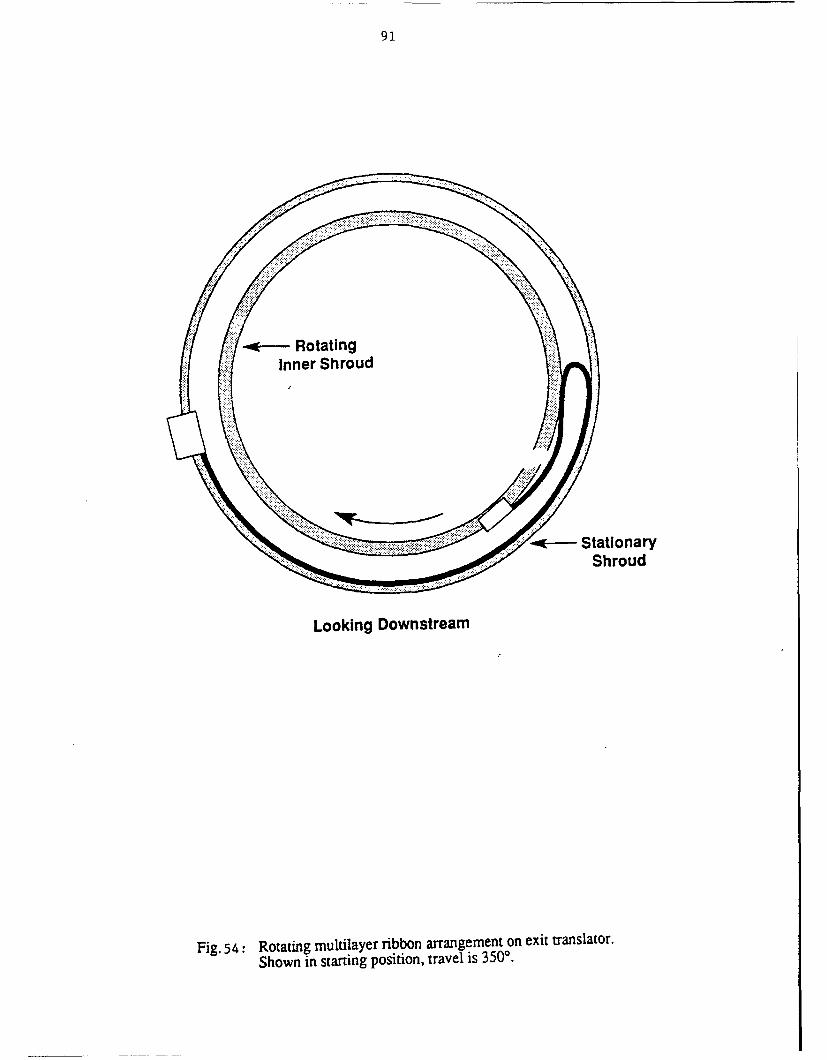
91
~- RotatingInner Shroud
... ... .4 StationaryShroud
Looking Downstream
Fig, 54: Rotating multilayer ribbon arrangement on exit translator.Shown in starting position, travel is 350'.

~9.
S.... .... ......... . ..........~
•. . -. •. -,7 • -. ......, ..! ! • ? !• !? ••!!!.,
:•i~ii~ i i • • ...... ..... ..
Fig. 55: The exit rake cabling became entangled in the translator chain driveduring the first test.

93
.......
Ma I0t
Vaall
rQQ

94
I I
...... ... ....... 4ol
....___ ........ ...___ ......... .. .
..... . ......
........... ..... ..... ....... .. ......
.......... .. .... ... ... ... ... . .......... ..... ............ ......in0
E0.... ... .... . ... ... .. .... ... .. ... ... ... .... .. . ........ ... ... ...
........ ........ ..........-.........r~en
.......... ............. ......... ... .... 0
.. .... . .......... .... .. .. .......... .. ..... ........ .. .
(_492p dw2o0Ln
..... .... .. ..... .......
............... o 0 ....... .. ...... .............. ...
... .. ..... ... .. .. .. ... .. .. ... .. .. .... .. ... .. ...
....... ... ... .. ... ... ...
..... ... .. ..... .
.j2D0 . ... ... .... ... ..... .. . " . .... ... .... .. ...
GJ~'p) dw, 1
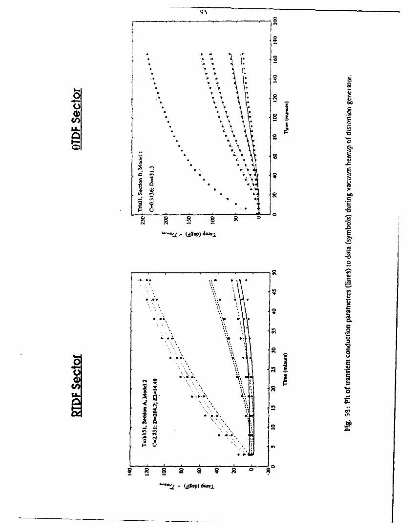
95
I �
* 4 �
*' - 41* *1�* ** .
4 p. .J� S.-04 4. I** 4� I,* U4 4
4 4 '4 I)
* L C0) 4. 4 I.
* .- �S 0LI� 4 . -�
i� 1.4 9. 4.
4. a4.. (U
* - - *4 U
4 4�44��
* 4.4
4 ...
.� * 9,44.
v� A-� 4 cc
- 4 4 n
I-c.) * 0� ----- -0 tj�
S- (�fS@p) dux� E
(U(UV0
9�
-4. 44 '� . p 4
* 6.�*4u ,.. .' . 4.1* ', E0* i
* .4 ,.� 4*
* . V. �.
9., 0
* 4.. � 4
* . 9* 44 V * - LI3 4*9A
-� 4.)U,
4..I., � * A
w
0�, 4'.'..
4.....I! *... cc- - V.4
C
* V.,
S..
� *� � a
- (A��p) du3.L
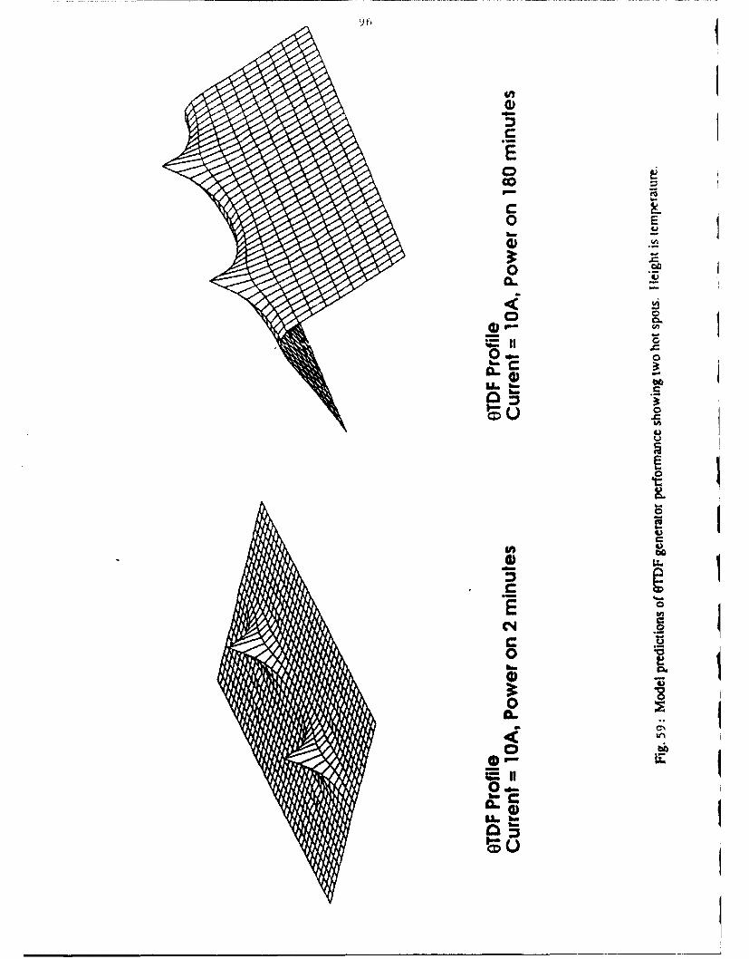
S~E
co
0E
0 SP
9-
C
o o
041
3: I
0,,
Lo
uU

97
TASK I: ASSESSMENT OF UNSTEADY LOSSES IN STATORIROTORINTERACTIONS
(Investigators: M.B. Giles, G. Fritsch)
Gerd Fritsch, the graduate student who was working on this project, completed his Ph.D.
thesis in May 1992. The thesis was subsequently prepared as an MIT Gas Turbine Laboratory
Report (GTL Report No. 210, "An Analytical and Numerical Study of the Second-Order Effects
of Unsteadiness on the Performance of Turbomachines") and is available on request. In June, a
paper was presented at the ASME Gas Turbine. Conference in Cologne. This focussed on the loss
mechanism due to the unsteady Stokes sublayer, as discussed in previous annual reports. A copy
of the paper is given as an Appendix. A second paper based on Fritsch's work is now in
preparation for the 1993 ASME Gas Turbine Conference in Cincinnati. This addresses the
analysis of time-averaged and space-averaged mixing loss which was discussed in last year's
annual report.
Overall, Fritsch's research has made an important contribution towards the growing
understanding of the impact of unsteadiness in turbomachinery flow. He has shown that the loss
due to unsteady circulation is very small and can be disregarded in future research. He has
explained and analyzed the mechanism of the unsteady Stokes layer loss. Unfortunately, he has
not been able to accurately assess its magnitude under typical engine conditions but even in this he
has made the important contribution of showing the limitations of existing CFD methods in
addressing this important question. Finally, his analytical work on the mixing loss ties together
and expands upon the work done by others and shows the separation of the loss due to different
forms of unsteady wave. It also highlights the loss that is introduced in steady-state multistage
CFD analyses using mixing plane coupling.
Also presented in last year's report were ideas for continuing this work in the future using a
combined asymptotic analysis of unsteady multistage flow fields. In the analysis, the base level is
a steady-state multi-row calculation using mixing plane coupling at all stator/rotor interfaces. The
next part is a calculation of the unsteady flow field using a linear perturbation assumption. The

I
third stage calculates the change in the time-averaged flo, field due to quadratic terms associatcd
with the linear unsteady flow field. A paper was presented on this idea at the ASME Gas Turbine
Conference in Cologne (also included in the Appendix). A number of related issues were also
discussed at a Workshop on Unsteady Losses held at NASA Lewis in May. This brought
together researchers in NASA, academia and industry to discuss the key aspects of unsteady flov,
in turbomachinery, to review our current understanding and the issues that need to be resolved,
Discussion of this is given in the section on Interactions.
Work on the multi-stage analysis will be continued by Dr. Giles at Oxford University, to
which he moved in June.
I!I

99-
THE AMERICAN SOCIETY OF MECHANICAL ENGINEERS 92-GT-389-345 E.47 St.. Now York.N.Y. 1001?
The, Society shrll not be eosponi~sblo lot ,tatisvints of Ooklinf 5 dvariew ;al P40fs of in 046C S ~~~Cussion 41 meet11nol of ithe S cellr of Ms Diiwsions re 0-ctiofn, 01 peinti i Itts putiwati
Dics toaninisd onyi 0 iw opJ se i ASME J~ný iviwws
G o- from ASAAF lot fifteen mtonihs afteittha mtteeting. .-
Second-Order Effects of Unsteadiness on thePerformance of Turbomachines
GERD FRITSCH-MICHAEL GILES
Department of Aeronautics and AstronauticsMassachusetts Institute of Technology
Cambridge, MA 02139
Abstract re average kinetic energy in a convected framens coordinate normal to a blade surface
A 2D, linearized approach is used to investigate second-order P pesreffects of unsteadiness on the time-mean efficiency of turborna- J entropy, surface coordinate, surface lengthchinery. The objective is to quantify unsteady losses with a itimenonzero time-mean and to examine numerical simulations with it/V velocity in the direction x, i, or s i ' or n~respect to the modeling of unsteady flow fields and loss mech- Z, i axal/ streamwise coordinate, convected z-coord.anisrus. Results of simulations constitute th~e input to the ana- $%~ coordinate normal to z, ilyticai models- employed.
Two unsteady loss mechanisms, one- of inviscid and the-other V~, V. inieant Machnd mbresece acoustic inenstyof viscous nature, are cousidered. The unsteady circulation F, A6. mach Match inuabneers frame) (P =/ P colosses, ice., the transfer of kinetic energy into the unsteady part j picithnacovtdfae(P cs,of the flow field through vorticity shed at the trailing edge of a W( ) real part of a quantityblade, was first considered by Keller (1935) and later by Kemp Re Rey-nolds number based on chord,and Sears (1956). The vorticity is shed in response to an un- Re,, Re* Re based on surface length, momentum thickesssteady blade- circulation and determined from Kelvin's circula- a3! average nondimensionaL entropy risetion theorem which is valid in compressible homentropic flow, rT,Z. mean convection velocity, velocity at .be hi. edgeUse of a numerical simulation to obtain circulation amplitudes yJR rotor speedavoids the limitations of thin-airfoil theory and yields results Greek Sy-mbolsmore realistic for modern turbomachinery. For the unsteady vis- Q angle between mean flow and axial directioncous loss mechanism, ie., the dissipation in an unsteady bound- inter-blade phase angle, attenuation factorary layer on the blade surface, Lighthill's high-reduced-frequency inter-wake phase angle in. convected framelimit (1955) is used to obtain the local velocity distribution in 7 ratio of specific heat, vortex street strengththe laminar sublayer and the corresponding time-mean unsteady 6, $/ steady and unsteady boundary layer thicknessdissipation-. The input- to the model is the time-harmonics of the la Irninar, SUblaye~r thickness in turbulent- flowpressure gradient along a blade surfacer obtained. from a simula- js, v, Pit viscosity, kinematic viscosity, conductivitytion. A numericaL study of theee..ors introduced b7- a. departure 7r- total priessure- ratiofrom the-higha-rvduced-frequency lEmit is presented. Losses from e smoothing coefficientboth, sources are found to be small. 178 ietZropic efficiency
p densityoT normal stress, shear stress
Nomenclature perturbation potentiala angle between wave vector ard surface normnal
Latin Symbols AA a reduced frequency A. = ik,,,, wavelengtha speed of sound W, cW/ angular frequency, blade passing frequencyc blade- axial. chord
C10Specific heat at constant pressure r circulationhtotal specific enthalpy of a fluid A difference, grid spacing
k, k.~ and k,. wave number, reduced frequencies 4 dissipation function
piten"eI-ge IttO IftueustiflniGe. Turbine and AoroenginisCongrses end uroositiolcologne, Gerntivir June 1-4, 1992

I 0
Subscripts a whole turbine under unsteady operating conditio, rrpod•-e at the boundary layer edge ing the whole range of unsteady effects, will rema~r impruactical
integrated for routine design purposes.in steady uniform fluid state far.upstream One of the main impulse& for ti" investigtiwn waI the dtve]
mixed mixed-out state far-downstream of the rotor opment of the CFD-code UNSFLO by Giles (1987, 1990, 1991a)out unsteady nonuniform state at the rotor outflow and the visualization package VISUAL2 by Giles and HamesJ isentropic (1991b) , which provides a detailed picture of unsteady flow phe-s at the wall nomena. Those include wake/blade row interaction, unsteady
shock wave structures, unsteady boundary layers, unsteady heatD, T design, turbine transfer, and unsteady vortex shedding. There is a need to un-HFL high-frequency limit derstand the physical nature of these phenomena, to quantify
1,2 first/Isecond-order (perturbation) their effect on the time-mean efficiency of turbomachinery, andto examine the modeling accuracy of CFD-codes with respect to
Superscripts these phenomenaunsteady quantity An alternative to nonlinear unsteady simulations, which isA complex-am plti-en nreceiving increased attention, are linear perturbation methods
A nonlinear steady state is found and the unsteady p 'ntisin G" . :
flow field superimposed upon it as a small perturbation. Second-Introduction order terms, i.e., terms quadratic in unsteady quantities, are ne-
glected since the perturbations are assumed to be small. LinearFlow fields in turbomachinery are inherently unsteady. In a perturbation codes have been found to give accurate results upturbine, the first blade row will be subject to a nonuniform di'- to a surprisingly high level of unsteadiness (Hall and Crawley,tribution of velocity and total temperature due to incomplete 1987; Lindquist and Giles, 1991) and will be more widely used
mixing in the combustion chamber. The relative motion of two in the future. Linear codes, like steady codes, cannot captureadjacent blade rows, in conjunction with the spatially nonuni- unsteady losses. The time-mean of the first-order unsteady dit-form pressure field locked to a loaded blade, leads to an unsteady sipation is zero; only terms second-order in unsteadiness have apressure distribution through potential interaction. A blade row nonzero time-mean dissipation.may move through and interact with the shock system originat- The turbomachinery community is moving towards the con.ing at the trailing edges of the upstream blade row. Stator sensus that increased losses under unsteady operating conditionswake/rotor interaction causes unsteadiness in the rotor frame of are primarily due to nonlinear effects like the alteration of thereference because the rotor is moving through and chopping the boundary layer characteristics through their effect on transitionwakes. Similarly, secondary flow effects like horse shoe vortices, (Hodson, 1983), the variation of secondary flow generation inpassage vortices, and tip clearance vortices contribute to flow downstream blade passages and their effect on separation or
unsteadiness. The viscous flow past a blunt turbine trailing reattachment. Nevertheless, the magnitude of effects that canedge results in vortex shedding; trailing edge vortex shedding be treated in a line.r framework, remains undetermined. Whilehas also been found in compressors operating in the transonic the corresponding unsteady losses are small by definition, theiror supersonic regime. Finally, there is unsteadiness induced by exact magnitude is of importance to the design process. Smallthe motion of the blades themselves, i.e., blade flutter. changes in the aerodynamic performance figure significantly over
Nevertheless, the standard aerodynamic design tools for tur- the lifetime of an engine. In a turbine, for example, efficienciesbomachinery are steady state codes both inviscid and viscous, often exceed 90% and improvements will be incremental.and steady cascade experiments. Designing a single stage or This paper treats two aspects in a 2D, linearized framework.blade row with steady state tools amounts to placing the stator In the first part, it revisits the Unsteady Circulation Losses firstand rotor infinitely far apart thus eliminating the effects of blade examined by Keller (1935) and later by Kemp and Sears (1956).row interaction and the interaction of convected disturbances Keller estimated the unsteady circulation amplitude to arrive atwith the downstream blade rows. Unsteadiness, however, con- the average kinetic energy in the unsteady part of the flow fieldtributes additional losses with nonzero time-mean. First, the induced by the vorticity shed at the trailing edge. Sears andenergy associated with the unsteady part of the flow field is Kemp used thin-airfoil theory to obtain the unsteady circula-usually not recovered in the blade passage or in downstream tion amplitude. This approach, while enabling them to calcu-blade rows; it will eventually be lost to viscous dissipation. Sec- late the circulation amplitudes, limited them to incompressibleond, the interaction of the unsteadiness with boundary layers flow, blades of zero thickness and camber with the mean flowand shock structures can trigger additional dissipation (Hodson, nearly in the blade direction, i.e., lightly loaded blades. Thus,1983; Ng and Epstein, 1985). In a steady viscous simulation, the the airfoils are more representative of compressor blades thaneffects of unsteadiness and unsteady viscous dissipation on the turbine blades. Furthermore, they had to specify the steady liftefficiency are not captured. An unsteady nonlinear simulation distribution on the blade. In this paper, the fluctuation am-is still prohibitively expensive for routine design purposes and plitudes are the result of CFD-simulations, which allows one towill likely remain so for the foreseeable future, in particular for obtain fluctuation amplitudes for arbitrary blade and stage ge-multi-stage turbomachinery Furthermore, the weakest point of ometries, steady lift distributions, and Mach numbers. Kelvin'sany numerical simulation, steady or unsteady, is the accurate circulation theorem, upon which Keller's work rests, is validprediction of losses and heat loads due to the unavailability of even in compressible homentropic flows. Eliminating the needadequate turbulence and transition models. Testing of a stage or to estimate the fluctuation amplitudes or to deduce them from

thin-airfoil theory, results in a more realistic measure for the sec-ondary kinetic energy in modern turbomachines and the losses Iassociated with its dissipation. The dissipated energy is relatedto the efficiency through a control volume argument and thelinearization of the unsteady isentropic efficiency. Examples aregiven for several blade rows and stages.
The second part considers Unsteady Viscous Losses, thatis, dissipation in unsteady boundary layers on the blade sur- U, 7fM, a y ]5faces. Using linearization, Fourier-decomposition in time, and "'a YLighthill's high-reduced-frequency ILmit, the momentum equa- I /tion, driven by the harmonics of the pressure gradient obtainedfrom a simulation, yields the local velocity distribution in the claminar sublayer. While a numerical simulation has difficultiesin accurately predicting the losses, the pressure distribution ispredicted accurately in attached flows. The second-order dissi-pation function with nonzero time-mean is calculated from the Figure 1: A cascade with unsteady lift and circulationinduced velocity distribution and the corresponding entropy in-crease integrated over the blade surface. The analysis can be ,.(z,t) convected with the mean flow is related to the rate ofregarded as a viscous complement to Johnson et al. f1988), change of the circulation bywho studied the surface heat transfer fluctuations in response toshock wave passing. The results of a numerical study to check I d(z ) = (r. -t -z.nP (2)
the errors introduced by a departure from the high-frequency .'t).l. U ()
limit are discussed. The model is applied to a transonic tur- With equation (1) and the convected coordinate i z-Ut, thisbine stage. Comparing the entropy rise due to unsteady vis- th equxpressed in the formcous losses to the total entropy rise in the simulation, it is seenthat unsteady viscous losses account only for a smalal part of ()=i k .epik . 3the increased losses under unsteady operating conditions. A c,(•) = ic k exp i(k. + 1/,,) (3)simple analytical model for the propagation of pressure wavesin a CFD-simulation is used to show that the principal loci of in the convected coordinate system (i,j). The reduced fre-
unsteady dissipation in a simulation may not be in unsteady quency k, = WmC//7 is defined with the blade axial chord c;
boundary layers as in real flows. Due to the action of numerical 0,,, denotes the inter-wake phase angle of the mth mode. In the
smoothing, dissipation within the blade passage can dominate, stationary frame, the linearized equation for the perturbationpotential 0 describing the vortex sheet far downstream of thetrailing edge, is
Unsteady Circulation Losses
Theory (8Ti a,where a denotes the speed of sound. It does not describe per-
Figure 1 shows a cascade in which every blade is experiencing an turbations convected through the blade row. The unsteady andunsteady circulation due to the presence of and interaction with convective contributions are eliminated by a shift to the con-the upstream blade row in an elementary stage. The derivation vected frame of reference; all that remains isproceeds along the lines of Keller (1935). The coordinate systemihas been chosen such that the mean velocity V7 far downstream + a = 0 .is in the a-direction; the vortex sheet shed from the nth blade (5)is located at yc = A,. P is the blade Pitch, P the rtated Pitch In the convected frame, the perturbation potential satisfies thethe convected vortex sheet an d the aneit direction. equation for steady irrotational flow. Due to the linear nature
of equation (5), one temporal mode can be treated at a time.The circulation of the nth blade is given by The periodicity condition for the mth mode is
.r. )r + rr,. exp {-5W tij~) (1) - n+fl.,))xpii~ (6)
with 6,, being the inter-blade phase angle for the mth mode. The potential for 0 <5 j t, is of the form
The frequenries w,M correspond to the blade passing frequency #I Ai +w, and its harmonics. The real part of any physical quantity is cosh k - A,) +
implied by complex notation. The strength of the unsteady vor- c
tex sheet shed at the trailing edge is determined by the condition i, sini (hm- - -)) exp Ji(kj + ±)' (7)
that the sum of bound and shed vorticity remain constant. This \c " 2
is a consequence of Kelvin's circulation theorem, which is valid wk, Tfor any compressible, inviscid, and barotropic fluid with conser- where A,,, is defined by A,, = . The values of the com-vative body forces acting on it. The strength of a vortex sheet plex amplitudes A,,. and h. are determined from the matching
3

102
conditions at ! = 0. First, the jump in the strearmwise velocity The subscript 'in' refers to a uniform and steady state far up.perturbation E,_ at y = nfi must equal the strength of the nth stream of the stator while 'out, s' and 'out' refer to the un-vortex sheet. Second. there must be no jump in the normal ve. steady spatially nonuniform rotor tofiow in a:.locity perturbation ,V_ across it. Using the periodicity condition isentropic expansion and in the actual expansion. respectiveIN(6) to relate the velocities at (i,0-) to those at (iP-, the Linearization of (12), calculus of small variables, and definitionperturbation potential becomes of an isentropic 'design point efficiency' between the steady and
uniform states 'in' and 'mixed',0/ icoshhAsin cosh k( _ -(
sin • + sinth' A- 2 nc -o _ = u, (1,!
2 \ c /J !, c- J+ sink ),, Cos sinhk. Am e~,) xp (i(k.,Ai + )6 . (8) (puhX. - (p),, h,,,,7.;.D
2 t C 2J lead to the result
Efficiency Drop A -7.,r . AS. (14)
The average kinetic energy per unit mass associated with the rT.D -
convected vortex sheet is The 'design total pressure' ratio 7r,,D is defined as
Tim =1l)} fR , [ m m )' 2 Equation (14), in conjunction with (11), tells how much of the"k2vo 2co ' d di departure of the isentropic efficiency from unity can be ascribed
1 r, A,,. sinh ý, cosh X_ to the dissipation of unsteady vorticity downstream of the rotor
4 )2 sin 2 & + sinh 2 A_, ( outflow. An analogous result can be derived for a compressor
stage. Details of the derivation for both turbine stages andwhich coincides with the result of Keller (1935). R denotes the compressor stages are found in Fritsch (1992).real part of a complex quantity. Questions relating to cross-induced contributions in the kinetic energy from disturbancesconvected through the blade row, which were brought up by Results - Unsteady Circulation LossesKemp and Sears (1956), are addxessed in Fritsch (1992). They The model described in the previous section was applied to awill not be discussed here because they do not bear heavily on number of blade rows and stages. The amplitudes of the un-the conclusions drawn. steady circulation were calculated with the CFD-code UNSFLO
It is assumed that the kinetic energy associated with the by Giles (Giles, 1987, 1990; Giles and Haimes, 1991a). It uses anunsteady vortex sheet cannot be recovered downstream. If this explicit Lax-Wendroff scheme to solve the unsteady compress-kinetic energy is lost to viscous dissipation in a constant area ible Euler equations in 2D on an unstructured grid composedduct, the average entropy rise per unit mass for an ideal gas of triangular and/or quadrilateral cells. Its quasi-3D capabilitywith constant specific heats -y is accounts for a varying streamtube thickness; arbitrary pitch ra-
........ d , (PUS)tios are handled by a time-inclined computational domain. The. (7 - 1) T ---. (10) simulations were run until the flow was periodic; then 50 instan-cl (Pu).fi..d . taneous flow solutions equally spaced in time were stored, from
The subscript 'mired' in equation (10) denotes the uniform state which the circulation amplitudes have been determined.after mixing; the overbar implies a mass-average taken beforethe mixing process that dissipates the kinetic energy. Equation(10) holds regardless of the mean-flow Mach number V and in Single blade row simulationsthe presence of unsteady waves other than vorticity waves, like This section combines the results of simulations for three differ.pressure waves or entropy waves. The entropy rise associated ent rotor blade rows with incoming wake disturbances modeledwith dissipation of the kinetic energy (9) is at the inflow boundary. The wake parameters were chosen from
-(. sinhA cosh Am the experimental data for the respective stages; no effort was42 r -n A -. s ini cs . (11) made to account for the viscous decay of the wakes in the exper-
iment. Potential disturbances were also simulated, but their ef-
In spatially nonuniform unsteady flow, it is the mass-averages of feet was found to be comparably small due to the Mach numberstotal pressure and total temperature at inflow and outflow that and axial gaps in the corresponding experiments. The numer-are needed to determine the isentropic efficiency. As iixing oc- ical implementation of wake models and potential disturbancecurs downstream of the rotor (or stator) exit, more losses are models is treated in Giles (1988).generated and the mixed-out uniform and steady state leads to Hodson (1984b) conducted measurements of wake-generateda lower total pressure. If the energy associated with unsteadi- unsteadiness in the rotor of a large-scale, low-speed, single-stage,ness is not recovered then it is the appropriate state to use in air-driven turbine. The 51 rotor blades are separated from 36the isentropic efficiency. The isentropic efficiency for unsteady stator blades by an axial gap of about one rotor axial chord. Anonuniform flow in an elementary turbine stage with adiabatic corresponding inviscid simulation of the 2D wake/rotor interac-blades is tion has been presented by the same author (Hodson, 1984a);
(puhz),, - fo' (puhh,)., d(*) the incoming wake was modeled after the experiment (Hodson,
(puh,),, ý-ph),,° d(*) (12) 1984b). The wake model in the simulation for this case, case
4

103
version of the rotor profile was investigatdd at Oxford UniversityA of table 1, was identical to his and the ma.imum velocity (Ashworth et al.. 1985; Johnson et al.. 19Y) . In the sinuia-defect and the wake width were chosen such as to replicate the tion, stator and rotor row are separated by an axial gap of 40tmaximum velocity deficit and the momentum deficit in the ex-periment. rotor axial chord and the rotor operates near the aesign inflow
angle of 58*. The outflow of rotor and stator row are supersonic.Case B is a simulation of the flow through the rotor of a producing weak oblique shocks at the trailing edges. A detailed
large-scale, axial-flow turbine model investigated experimentally computational account of the inviscid stator/rotor interactionby Joslyn et al. (1983). It is 4 one and one-half stage turbine for almost identical input parameters was presented by Gdesmodel consisting of 22 first vanes, 28 first blades, and 28 sec- (1990). The oblique shock wave originating at the nozzle gulideond vanes, representing the first three blade rows of the high vane trailing edge first hits the downstream rotor around thepressure turbine of a high-bypass-ratio aircraft turbine. The crown of the suction surface and is reflected from there. Subse-Reynolds number as well as the absolute and relative flow an- quently, it moves forward to the leading edge with the reflectedgles are typical for current high-pressure-turbine airfoils. The portion impinging on the pressure surface of the adjacent bladewake profile at the rotor inflow boundary was Gaussian (Giles, and being reflected to the suction surface once more. Upon lift.1988). Wake width and maximum velocity defect were chosen to ing off the rotor blade, the primary shock wave grows in lengthmatch the maximum velocity defect and the momentum defect until the relative motion of the blade rows causes it to strike themeasured at midspan downstream of the first vane. next rotor blade. In the mean time its reflection off the rotor
Binder (1985) used the L2F-technique to measure the flow leading edge has impinged on and reflected from the nozzle guidein a cold-air turbine. The stage has 20 stator blades, 31 rotor vane suction side. Comparatively large unsteady amplitudes forblades, and an axial gap of 113% rotor axial'chord; it is a scaled this strong interaction are expected and have been reported forversion of the first stage of a helicopter gas turbine. The flow this turbine stage (Giles, 1990). The increased importance ofin the low-aspect ratio, high hub-to-tip ratio stage is weakly higher harmonics is a consequence of the discontinuous naturetransonic and the experiments showed a wake with a velocity of the shock waves.defect of 6.5% at midspan 50% rotor axial chord upstream of the Parameter ACE Stage 67rotor leading edge. Based on the measured velocity distributionat the rotor inlet plane, a sinusoidal 'ake model (Giles, 1988) stator inflow angle 0" -44.70
with a maximum velocity defect of 6.5% in the stator frame was stator outflow angle 73.5" 3.5'*
chosen for the simulation of the flow through the rotor (case C). rotor inflow angle 56.7" 59.91rotor outflow Angle -67.6' 39.7'
Parameter Case A Case B Case C stator inflow Mach number 0,14 0.67
inflow angle 2.1" 48.9' 46.7" stator outflow Mach number 1.13 0.46outflow angle a -66.8" -65.5' -62.0' rotor inflow Mach number 0.59 1.11inflow Mach number 0.14 0.12 0.43 rotor outflow Mach number 1.16 0.62outflow Mach number 0.40 0.20 0.65 rotor speed VR 0.55 0.83rotor speed VR 0.31 0.11 0.58 reduced Frequency k' 2.38 (rotor) 21.5 (stator)reduced frequency k, 3.45 2.92 4.25 circulation ri/ro 2.19% 0.90%wake velocity defect 4.6% 15% -6.5% 5s/Fo 1.02• 0.80%Wake width/stator pitch 30% F 10%r - - -3. j 0.20% '0.49%circulation r1/ra 0.67% 0.57% 2.83% r4/ro 0.25% 0.14%entropy rise AS 1."0-6 1.2.10-s 027"1- enrpTieA5,•11*1- .. 4.0 * 10-'
efficiency drop Ai.,r/'i-r> -0.04% -0.11% -0.24% efficiency drop A11./i.,D -0.30% -0.03%
Table 1: Results for single blade row simulations Table 2: Results for single stage simulations
The results are summarized in table 1. Mach numbers and The compressor stage is known as NASA stage 67. It is aflow angles are mixed-out averages in the rotor frame. Un- low-aspect ratio, single-stage, transonic, axial-flow compressorlisted higher harmonics of the circulation are a factor 10 or more designed and experimentally investigated at the NASA Lewissmaller than the first harmonic. Research Center (Hathaway et al., 1987). The stage consists
of 22 rotor blades separated from 34 stator blades by an ax-
Single stage simulations ial gap of 78% rotor axial chord. At a rotor tip Mach numberof 1.38, strong shocks are present in the rotor passage. Shan.,
Two inviscid simulations are presented here; one for a turbine (1989) used UNSFLO to calculate the flow through the sta!-e
stage and one for a compressor stage. In contrast to the previous at midspan with the input parameters inferred from the experi-
three cases, the unsteadiness acting on the downstream blade ments at NASA Lewis. The case considered here is a full stage
row is not prescribed but the result of blade row interaction in with purely potential interaction between the blade rows. The
the simulation. Viscous wakes and their subsequent interaction magnitude of the potential interaction strongly depends on the
with the downstream blade row, some aspects of which could be size of the axial gap separating the blade rows. A wide range of
modeled inviscidly, are not included, gap sizes exists in compressors and the gap itself varies hub toThe turbine case considered is a highly loaded transonic high- tip. For the case presented here, the gap was 10% of the rotor
pressure turbine stage, often referred to as the ACE turbine axial chord. The shock position is roughly 30% rotor axial chordprsse, turinhwastestae, ofteT referred eto al., the 8). AC tu e downstream of the rotor leading edge and there is no significantstage, which was tested at MIT (Guenette et al., 1988) . A 2D-
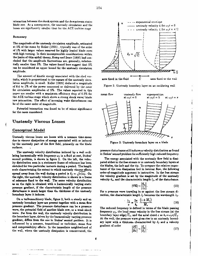
104
interaction between the shock system and the downstream stator .... exponential envelopeblade row. As a consequence, the unsteady circulation and the - unsteady velocity t for wft = 0losses are signifcantly smaller than for the ACE turbine stage. - - - unsteady velocit. i for wft = 7•2
Summary g
The magnitude of the unsteady circulation amplitude, estimatedat 5% of the mean by Keller (1935) , typically was of the order rI,of 1% with larger values reserved for highly loaded blade rowswith high turning. In their incompressible considerations within L \ i= / \the limits of thin-airfoil theory, Kemp and Sears (1956) had con- .\cluded that the amplitude fluctuations are, generally, substan- -7tially smaller than 5%. The values found here suggest that 5%can be considered an upper bound for the unsteady circulationamplitude. S
The amount of kinetic energy associated with the shed vor-ticity, which is proportional to the square of the unsteady circu- axes fixed in the fluid U axes fixed to the wall
lation amplitude, is small. Keller (1935) deduced a magnitudeof 0.4 to 1% of the power consumed or delivered by the rotor Figure 2: Unsteady boundary layer on an oscillating walfor circulation amplitudes of 5%. The values reported in thispaper are smaller with a maximum efficiency drop of 0.3% for mean flow unsteady flow superpositionthe ACE turbine stage which shows a strong shock wave/ blade at wit = 0 at w't= 0 at wit =Irow interaction. The effect of incoming wake disturbances canbe of the same order of magnitude.
Potential interaction was found to be of minor significance
for the cases considered.
Unsteady Viscous Losses
Conceptual Model
Unsteady viscous losses are losses with a nonzero time-mean sdue to viscous dissipation of energy associated with or induced Figure 3: Unsteady boundary layer on a bladeby the unsteady part of the flow field, primarily on the bladesurfaces.
The unsteady velocity distribution induced by a wail oscil- pressure disturbance still induces a velocity distribution as found
lating harmonically with frequency w, in a fluid at rest, Stokes' in Stokes' second problem for sufficiently high reduced frequency.
second problem, is shown in figure 2. On the left, the veloc- The energy ass9ciated with the unsteady flow field is dissi-ity distribution seen in a stationary frame of reference has been pated either in the free stream or in unsteady boundary layers atsketched for two particular instants during a period. The length the blades, the hub and the tip. To compare the relative impor-scale characterizing the extent to which unsteady viscous effects tance of the two dissipation loci in laminar flow, the following
spread away from the wall during a period is 81 = Vr•'•. On order-of-magnitude argument is instructive. In the free streamthe right, the unsteady velocity distribution is shown in a frame the velocity gradient is set by the magnitude of the unsteadyof reference fixed to the wall. The same velocity distribution velocity ,i., and the characteristic length If, of the disturbance.
as on the right is obtained with a harmonically varying static 1VV (15)pressure gradient, if the characteristic length of the pressure ifdisturbance is much larger than thv thickness of the unsteady For a pressure wave traveling in or against the free stream di-boundary layer it induces. rection, the characteristic length Ij becomes the wavelength A,.
On a turbomachinery blade, figure 3, both a steady and an 2A (2 -unsteady boundary layer are present together with a mean flow - (16)pressure gradient. The pressure disturbance can be a pressure The reduced frequency is defined in terms of the blade passingwave, the potential field of another blade row, or a weak shock frequency w,, the local mean velocity in the free stream (at thewave. Far from the wall, the unsteady velocity distribution in boundary laycr edge) UT., and the axial chord c as k, =wic/1Ue.the boundary layer, driven by the harmonically varying pressure At the wall, the pressure wave gives rise to an unsteady bound-gradient, differs from the one in Stokes' second problem. It isinfluenced by a nonzero, transitional or turbulent, mean flow ary layer with a thicknesod characterized by , and a velocityand compressibility effects. In the immediate neighborhood of g n r I (1the wall, where the unsteady dissipation is concentrated, the OnI l-"6, (17
6

P) 5
The local average rate of unsteady viscous aissipation is propor- Linearizing the kinematic and the thermodynamic variablestional to the square of the velocity gradient. The extent of the around their time-mean (and nondimensionaliziri them by thefree stream, characterized by the axial chord, is much larger the local mean velocity and density in the free stream, the bladeunsteady boundary !ayer thickness. To obtain the integrated ef- passing frequency, and the blade axial chord), the first-orderfect of dissipation in the free stream and the unsteady boundary perturbation equations of the streamwise momentum equationlayer, these different scales have to be accounted for. Dissipation and the stress-strain relations take the formin the free stream is negligible if k'• 5uftL" Oil *Or
by2 t as Os On On
Q-)(TO < 18) _iý+ (aý- + On) + a'P + Of-~- - ,(24)
With the definition of 8i and equation (16), (18) is rewritten as 21 •)=X- \ = / On (25)
4'vi (1 = , •1 (19) oreuntdydsiainfnto wihulketsir-
Z72 Re 2 The laminar viscosity y has been assumed constant. The second-order unsteady dissipation function $2 which, unlike its first-
where the Reynolds number is defined in terms of mean free order counterpart, has a nonzero time-mean, isstream quantities as Re = / For the Reynolds numbersencountered in turbomachinery, this inequality is always satis- O2=12 1 at, ain +"fled and dissipation in unsteady boundary layers dominates over We' TS On Os andissipation in the free stream. Unless the level of the tu-julentviscosity in the freestream far exceeds the one characterizing the -2 U. + (26)boundary layer, inequality (19) also holds in turbulent flow. (3 TO On )
Theory - Unsteady Viscous Losses The high-frequency limit is characterized by a reduced frequency
The initial step in the analytical approach is to linearize the k' > 1. (27)
governing viscous equations around their time-mean. Taking As a consequence,the first-order perturbation equations to their asymptotic high-frequency limit, the momentum equation yields the unsteady by/F 'C 1, (28)streamwise velocity distribution. From the unsteady velocities in X/c 1 I, (29)the boundary layer, the time-mean of the dominating term in the and Sf/At .t 1 (30)second-order unsteady dissipation function 42 can be calculatedand related to a change in the time-mean isentropic efficiency. hold in the high-frequency limit. Inequality (28) implies that
The problem is described in a Cartesian coordinate system normal derivatives of unsteady quantities dominate over normal(s, n) where the coordinate n is aligned with the local surface derivatives of steady quantities, because the unsteady boundarynormal. The governing equations are the continuity equation, layer thickness is much less than the thickness of its steady coun-the streamwise momentum equation in conjunction with the terpart. Inequality (29) allows one to neglect streamwise meanstress-strain relations, flow derivatives because the wavelength of the disturbance is
much less than the axial chord which characterizes mean flow"O + Uj (p + !L"- + 0- , (20) gradients. In other words, parallel mean flow is assumed and the
p Os On streamwise evolution of the steady boundary layer is neglected.2 Ou Os_ (n + &2 Inequality (30) implies that the wavelength of the disturbance3% \ •p 2•, - I •' ( = T + ' is far greater than the unsteady boundary layer thickness. It
allows for the neglect of unsteady streamwise derivatives in thethe energy equation in conjunction with the definition of the presence of unsteady normal derivatives; it always holds for thedissipation function 4,, large Reynolds numbers found in turbomachinery.
(0 +,' 0 O T =_ Op Op Op Taking the momentum equation (24) and the stress-strain,.ts-s, +) ,9 n relations (25) to their asymptotic high-frequency limits, the fol-
+ 8 \ + 1 (OT\ (2 lowing terms drop out: (7O + (KE)
80.' + O.,d =_f
a[su On O8s On (30) (29) (29) (28)
3 8s On P(32)+= + +P
and the equation of state. Due to the boundary layer character (30)
of the problem, the normal momentum equation is replaced by '° f a ý 8#the assumption (Op/On = 0). n
7

106
Numbers above the arrows refer to inequalities (27) to (30) due to the orthogonality of sines and cosines. The time-meanrand give the rationale for the neglect of individual terms. In- of the unsteady dissipation is calculated mode by mode andequality (27) leaves the unsteady term dominant on 'eleft-hand summed subsequently. For the m-th mode, the dissipat~on perside of the momentum equation. On the right-hand side, the unit volume isdriving unsteady pressure term and the unsteady shear term 1 i ___ ,•2 -remain. Substituting the stress-strain relation into the high- .2,- exp €€] n (34)frequency limit of the momentum equation, the velocity distri- 2mk, $ IIbution near the wall is described by the differential equation The dissipation is largest in the region of steep gradients near
the wall where the agreement between high-ftequency hmit and
S 1 1 = _-- _(31) exact solution is best. Therefore, equation (34) is integratedSRe •,• On2 ,from the wall into the free stream to obtain the dissipation per
Since (31) is a linear constant-coefficient equation, any distur. unit surface area.
bance can be decomposed into its temporal Fourier-modes. For ! / i 1 _,,the mth mode, the solution near the wall is 42s,^ =2 , \2--,Re k -7 9 (35)
-- I-exp (i-1) in a exp {-imt} (32) The difference in the integrated dissipation T2, between 0,e eX-Mkjp\. ( I act solution and the high-frequency-limit solution of figure 4 is
where P,, denotes the complex magnitude of the m-th harmonic about 10% of the exact solut, n. The effects of turbulent bound-of the pressure disturbance. Figure 4 compares this solution to ary layers, mean flow pressure gradients, and mean flow Mach
the exact solution for an upstream propagating pressure wave number are addressed later.over a flat plate with a laminar boundary layer. In the Stokes Unlike in the Unsteady Circulation Losses, the energy is not
dissipated downstream of the last blade row but in the blade28 passage. The mean flow state al 'ng the blade varies and the
potential region entropy rise per unit dissipated energy is not constant. Integra-24 .ticn around the blade surface and division by the mass flux ..
yielo the average specific entropy rise in the blade passage due20 .. .to unsteady viscous dissipation. In dimensional quantities it is20l ... ........ .........
,~l6 .. ~. _ 7-1) ~ d§ 2,,., (6n 16 -. ----1 ----.... . . .. ... .... .... ... ........ ......... ; .. ....... (36). . • ' - ):
bf12. outer region ............ -_ The average specific entropy rise is again related to an efficiency
drop, as in equation (14).S......... .........i ........ i......... ........ ... ...... .. .. ..... i....S--Results - Unsteady Viscous Losses4 ......... ....... ......... .............. ........... .i....... . ........
Stokes sublayer The model has been applied to the ACE-turbine stage described00 0.in the results section of the Unsteady Circulation Losses. The
002 0.4 0.6 0.8 1 1.2 1.4 1.6 1.8 input required for the model is the time harmonics of the lo-- exact solution ke = 9 cal pressure gradient along the blade surfaces. Those can be--- equation (32) e MVe = 0.3 the result of a viscous or an inviscid unsteady simulation. The
Figure 4: Unsteady velocity distribution aS a function of (n/62 ) dominating unsteady effect of rotor blade row/shock wave in-teraction is captured in an inviscid simulation. The parametersof the simulation were similar to the ones used before except
sublayer near the wall, the velocity distribution is well repre- that UNSFLO was run in the viscous mode (Giles and Haimes,sented by equation (32). The agreement increases with the ra- 1991L), the rotor speed was increased, and the back pressuretio 316j (which is proportional to V for a laminar flat plate was lowered slightly. This resulted in stronger stator trailingboundary layer). It decreases with the Mach number because edge shock waves and reduced the mean rotor incidence angle(32) assumes negligible mean flow at the edge of the unsteady to 480, matching the experiments of Johnson et al. (1988). Inboundary layer and incompressible flow. Due to the neglect of experiments (Ashworth et al., 1985) , the rotor boundary layerfree stream convection it asymptotes to the wrong velocity mag- was laminar over most of the suction surface for low levels of freenitude in the free stream. stream turbulence and in the absence of wakes and shock waves.
The dominating term of the unsteady dissipation function The pressure surface boundary layez was transitional. Bar pass-
62 in the asymptotic high-frequency limit is obtained from (26) ing experiments to simulate the stator wakes and shock waveswith inequalities (28) to (30). Taking its time-mean gives showed that widely spaced wakes and shock waves temporarily
trip the boundary layer, which will relax back to a laminar stateTR dt =after the disturbance has passed. For a bar spacing resembling
engine conditions, the boundary layer is transitional or turbu-
[ ( lent. In the simulation, the flow was prescribed turbulent from( the leading edge on.
8

Figure 5 shows the specific ,ntropy rise jue to unsteady vis. entropy rse through the stage " -.;rl the uvý,,escv , at. i
cous dissipation on a rotor blade surface. A value of s.4=0 ccr tiCase, tse a.sz of ofmas. nowenltim a&.': ene.'? 4,:e
responds to the rotor leading edge; positive and negative values averaged at the stator outflow boundary to provsde urlortu a.nd
correspond to pressure and suction surface, respectively. The steady rotor inflow conditions The (aonphysical) entropy r.
losses are concentrated on the suction surface between rotor at the interface, acc.ounts for about 20% of the total At a conse
leading edge and c-own, where the pressure gradient fluctuates quen :, the sientropic stage efficiency is 0.4% less in the steady
in response to shock wave passing. The integrated entropy rise sunuia•ion- Since the unsteadiness does not propagate br-t.:
for a rotor blade is A3= 2.8a10"; this translates into an effi. the steady interface, the entropy ries rnuci slower in the rotor
ciency drop of Ai..r/•?,r,D=-0.09%. These numbers afe subject passage than in the unsteady simulation Second. the entioiy
to errors examined in the foUownng section. Of the total, 64% is rise between rotor leading edge and crown, the region where the
at blade passing frequency and 14% in the first harmonic. unsteady losses ate concentrated, is about 10' for the steady
c&ae and 3.10" for the unsteady case The diference :4 much6 larger than the entropy rise that has been asershed to unsteady
leading edge: s = 0.0 viscous losses. Third, the entropy ec between crown and trsil
4 trailing edge: s = 0.9 r,,,,e-u , wla., ing edge as well a between traibng edge and outlet b•urciA'
16 ..... s .-..6 ,,..... ........ is significantly in the unsteady simulation. Ba•'rg tuibulexcenmodehng in the boundary layer as a reason for the steeper ne.
numerical smoothing acting oan the unsteadiness in the blade44 "• ..... .... • .... ...... ......... .... ............ ........ 4 u a e r m i s a h n y e p ~ a o4 ~Passage remaimns as the only explanation
104 -:
rotor crown Modeling Accuracy
2............ Loss...de
The derivation of the unsteady viscos. losaes involved four ap-
1 ........................ ................. proximations, each of which introduced errors The first two, the
:. . . boundary layer approximation and the linearization thereo will] not be examined. The errors introduced in the last two steps.
0 • the invocation of the high-frequency limit and the assumption-1.25 1 -0.75 -0.5 -0.25 0 0.25 0.5 0,75 of laminar flow, dominate.
surface length s In laminiar Sow, the two main effects not modeled in the
Figure 5: Entropy rise per unit surface length high-frequeacy limit are the compression of the boundary layerand the free stream convection. Even larger errors are due to thepresence of a turbulent mean Sow. To estimate the errors, a IDcode was written to solve the linearized equations for a flat plate
2.4 ........ ................ boundary layer, figwr 7, subject to a pressure wave propagatingrotor crown at an arbitrary non-sero anle 0 relative to the suirface normal.
. .. . ntr. ln ce ... .. .g;. .....trl The parallel Sow assumption was retained because the evolu.
._.. ...... .... 7 .5 boundary ". .7I -1 6 . .. .. ... . .. . . ... .. .. ..... ........... . .. ". . . ..... "U H•_ stator trailing !i: •[/
------ ..... ....... 7 ........ ......... ...*........,0 .8 " .. .. ........ ........ ........ . ........ ....... .÷ ........ •......... .- .................
o~jrotor leadingedge.. ... ......... ............ ....
0 2.. .2.5unsteady laminar - turbulentsteady axil location z
Figure 6: Entropy rise in the steady and the unsteady simulation Figure T: Model problem for namerical error evaluation
Figure 6 shows the time-mean mass-averaged entropy rise tion of the mean flow boundary layer ta~ea place over a length
through the turbine stage in the simulations- The axial coor- scale much larger than the steady or the unsteady boundarydinate z is nondimensionalized by the stator axial chord; the layer thickness. This assumption combined with a small steady
stator leading edge is located at z = 0. Three observations can and unsteady boundary layer thickness (compared to the wave-
be made. First, the steady simulation, in which case the con- length), reduces the problem to one dimension. The boundary
servati-'n variables are averaged at the interface, has a higher was modeled as an adiabatic wall.
9

103
All mean velocity profiles were taken to be identical to the 12.rresponding profiles in steady flow. Only very large distuu Ret 3
ouance amplitudes (snd frequencies close to the turbulent burst- -k____=____
ing frequency) lead the mean flow pwfiles to deviate from thecorresponding profiles in steady flow (Kazlsson, 1959; Par'ich et&l., 1982) . In laminar low, the velocity profiles were obtained 0.8 ..................... ....... ......as the solution of the Falkner-Skan equations. In turbulent flow, *" 2"7a three layer model with the inner law in Spalding's formulation(Spalding, 1961) and a law of the wake in Coles' formulation 0.6 .........(Coles, 1956) was used. Both the laminar and the turbulent k ý2S .24 1velocity profile are strictly valid for incompressible flow only, 0.4 ......... .............. 7.but were used regardless of the free stream Mach number. The 98mean temperature and density profiles were obtained from the j9velocity profiles with the assumption of a unit Prandtl number. 0.2 .
The laminar part of the code was verified by comparison toLighthill's analytical work (1954) on oscillatory boundary layers 0in an incompressible mean flow. The turbulent part was first 0 0.1 0.2 0.3 0.4 0.5 0.6 0.7 0,6checked against the laminar solution for very high frequencies V.and then against experiments by Cousteix et al. (1977). Figure 9: High-frequency limit dissipation and full turbulent
The numerical error evaluation is summarized in figures 8 model dissipation . downstream propagating waveto 10. Figure 8 assumes laminar mean flow and pressure wavespropagating parallel to the boundary. It shows the ratio of the Re - 3.5WJRe. = 1002 42 .5 ............i ..... ...... ..... : ..... ........ .........i .......i .... ....
upstream propagating ji .jR, 0w2ve kt• • OS 0o /•', 1..
.. ... .......... .........-1 1. -Increasing it, 3,6
10 a.FIi0• ...... 1 .0 5 ......... 9.. ......... 0.. 2.77 .......... . ... ......
2.5 01b 0.1 2 034 05097 0
1"2' 7.•• ....... ....... ... \' ' : ]•e -"00•
0-.8 ........ ... ..... -- --- .. .. ....- ..........downstreami f l0.
0..propagating wa;ve"'•....."", '•=03 .909k, 0 25. it: .4i0 0.1 0.2 0.3 0.4 0.5 0.6 07 0'8
0 01I 0.2 0.3 0.4 0.5 06 0.7 0.80 10Figure 10: High-frequency limit dissipation and full turbulent
model dissipatios - upstream propagating waveFigure 8: High-frequency limit dissipation and full linearized
laminar model dissipation the ratio of the integrated dissipation calculated in the EFL tothe full turbulent dissipation for a Reynolds number Re.= 10'.
integrated dissipation Ia. calculated in the high-frequency limit As opposed to the cue in lamina low, the HFL is not exact(HFL) to the one calculated with the full linearized equations. in the limit (W.--40). This is because the turbulent nature ofIn the limit (19, -- 0) or (k,h-oo), the HFL model gives the cor- the mean Bow introduces additional errors into the HFL modelrect dissipation. The lower the reduced frequency for a nonzero which is an inherently laminar model. For high reduced fre.free stream Mach number, the greater the deviation. This is quencies, the turbulent dissipation again approaches the valuea consequence of the unsteady boundary layer spreading away of the NFL model although this is not evident within the rangefrom the wall into the steady boumdary layer where convective of reduced frequencies displayed. The parameter (3/11) is theterms in (24) become important. Depending on the direction of ratio of the thickness of the laminar sublayer of the mean flow,propagation, the HFL yields an integrated dissipation greater or dtfined as 301+ in wall coordinates, to the thickness of the un-less than the full linearized model. steady boundary layer. For frequencies such that (t/AA) >, 1,
The flows in turbomachinery are almost always transitional the unsteady boundary layer is confined to the laminar sublayerr turbulent and the unsteady boundary layer extents beyond and the HFL model gives accurate results.ne laminar sublayer. In figures 9 and 10 errors due to the as- The ratio (isJrxFLf4,) for a downstream propagating wave
sumption of laminar mean flow in the HFL model appear super- in turbulent flow behaves in a similar fashion to the correspond-imposed on errors due to finite reduced frequencies. They show ing ratio in laminar low. With higher reduced frequency and
10

i 09
lower Mach number,'the HFL is more accurate. The behavior of where the relation (k/k,)*S., valid in the limit (.L,00) ha-s(
42,,HFL/2.) for an upstream propagating wave, however, dif. been used. Alterrattvely, (41) can be expressed a
fers significantly from the behavior in laminar flow. In the limit(M.•-O), the ratio is less than unity and matches the value for a V2 (M./Re) (2v/)Xl) tan $.in 0. (42)downstream propagating wave. The laminar HIFL model under. The longest wave in a turbomachine typically has a nondimez-predicts the velocity gradients (and uses the laminar viscosity) Teonal wavelength At of order unity. Assuming Reynolds andand thus arrives at too low an integrated dissipation for finite Mach numbers typical of turbomachinery (and tan 0 sin P of or.reduced frequencies (or 31/16). As the Mach number increases, der one), O(103) reflections should occur before the wave am-this ratio rises above unity because the HFL overpredicts the plitude is halved. In an inviscid simulation of the flow throughunsteady velocity magnitude in the free stream; it is the rela- the ACE turbine stage no more than three reflections of weaktive magnitude of these two effects that governs the behavior of shock waves/pressure waves are discernible. The approxima-(Cil.apLIt,/ ) in figure 10. tions made in the derivation of the HFL model and in the above
The flow through the rotor of the ACE stage is turbulent and order-of-magnitude argument can not account for a difference ofthere is a strong favorable mean pressure gradient in the region two orders of magnitude. This suggests that numerical smooth-of unsteady viscous losses. Calculating the laminar sublayer ing in the free stream dominates over dissipation in unsteaG:thickness from the wall shear of the simulation, gives a ratio boundary layers.W1/6.,-:1.2. The free stream Mach number in the rotor frame is The propagation of a pressure wave in the uniform free stream(]W*;. -0.65) in the main region of unsteady viscous losses. There- can be modeled numerically by the convection-diffusion equationfore, figures 9 and 10 suggest that the unsteady viscous lossescalculated for the ACE turbine stage =Ar,/?,rTD 0.09%) are 85 (I ±H' -in -) ="AL - .A- IT (43)at most a factor 1.5 too large and could be up to five times at+ &si I "larger. where z is a coordinate in the direction of wave propagation; A
denotes the mesh spacing. The time t has been nondimension-Numerical smoothing alized by the axial chord and the speed of sound. NumericalConsider a pressure wave propagating through an unloaded flat smoothing, necessary to stabilize the code, has been added onplatcnsiader a ith pre ire wavepran ulow The inloadednflt pressu the right-hand side. The time-rate of decay of a wave amplitudeplate cascade with uniform mean flow 17,. The incident pressure due to second-order smoothing for shock wave capturing is
wave of figure 7, propagating at an angle 0 relative to the surfacenormal, is described by its wave amplitude A - d2 k' A. (44)
V = P exp { i k (a sin 0 - n cos 0) - i t). (37) In smooth-flow regions, second-order smoothing is turned off.where k denotes the wavenumber. Upon reflection at the blade There, the time-rate of decay due to fourth-order smoothingissurface, the wave will lose a small fraction P of its amplitude *o 64 - e, k4 AS. (45)dissipation in an unsteady boundary layer. The time-mean rateof energy dissipation per unit surface area is given by equation Assuming that a wave typically travels one aiial chord between(35) with the pressure gradient determined from (37). The time- successive reflections, the time between reflections is t z I formean rate of acoustic energy incident on the wall is given by the moderate Mach numbers. Therefore, P and f, also representacoustic intensity the amplitude attenuation caused by numerical smoothing be-
:1 1 tween reflections. Alternatively, they can be written asS2 P co- A. (38) ~ e A ,) and 04 ~- e4 A (2w/A 1 )4 (46)
The rate of acoustic energy reflected is which shows the strong bias of fourth-order smoothing towards
1 2 - 1 - short wavelengths. Typical values of the smoothing coefficients2 (1 ) l (1-•)I~M'.cose. (39) are (ea 10 -) and (e4 = 10). A standard value of the mesh
spacing is A= 3a 10-2. For the losgest wave with a wavelengthThe above acoustic intensities, strictly valid only for V. 0, are of order unity, fourth-order smoothing in between successive re-used for simplicity. Since the objective is an order-of-magnitude flections results in an amplitude attenuation that is an orderargument, these simplification do not compromise the subse- of magnitude smaller than the. attenuation caused by viscousquent conclusions. The streamwise velocity distribution in the dissipation in an unsteady boundary layer. For shorter wave-unsteady boundary layer induced by the incident and the re- lengths, numerical smoothing starts to dominate. The attenua-flected wave are nearly in phase because of inequality (30). The tion coefcient Pa of the sixth harmonic approaches unity for therate of unsteady viscous dissipation per unit surface area is above choice of A and c4. This implies, that numerical smooth-
,,= (2--fl)1 1 1 Jo'- ing dissipates wavea prematurely in the free stream unless theV2 2k.T, as (40) wavelength is on the order of an axial chord or more.The weak shock waves, whose interaction with the blade rowswhere incompressible meanuflow was assumed. Balancing incom- is the primary cause of unsteadiness in the ACE turbine stage,
ing intensity, reflected intensity, and unsteady dissipation gives are subject to strong numerical dissipation, even in the absencean estimate for the attenuation factor 6 of of second-order smoothing. The pressure gradients driving the
j3• = M, V R tan Gasin a, (41) unsteady boundary layer --e diminished by numerical smooth-ing, lowering the level of the predicted unsteady viscous losses.
11

11)
Conclusions M. B. Giles and R. Haimes, 1991a. 'Validation of americal Method for Unsteady Flow Calculations' ASME-Paper
This paper has studied two unsteady loss mechanisms for ge- 91-GT.271.ometries, Mach numbers and loading realistic for modern tur- M. B. Giles and R. Haimes, 1991b. 'Advanced Interactivebomachinery. The results of numerical simulations were used Visualization For CFD', Computing Systems in Engtneertng,as input to the 2D, linearized, analytical loss models. Losses Vol. 1, pp. 51-62.from both mechanisms are small compared to other (nonlinear) G. R. Guenette, A. H. Epstein, N1. B. Giles, R. Haimes, andsources that increase the losses under unsteady operating con- R. J. G.Norton, 1988. 'Fully Scaled Transonic Turbine Rotorditions, like a change in the transition point, and compared to Heat Transfer Measurements', ASME Paper 88-GT-171.the uncertainty in measured efficiencies. Since this paper is 2D, K. C. Hall, and E. F. Crawley, 1987. 'Calculation of Un-it does not account for possibly important 3D effects. steady Flows in Turbomachinery Using the Lineari•ed Euler
Equations', Fourth Symposium on Unsteady Aerodynamics andThe Unsteady Circulation Losses, which are a due to vis- Aeroelascity of Turbomachines and Propellers, Aachen, Ger-
cous dissipation of kinetic energy associated with vorticity shed many.in response to circulation variations, resulted in an isentropic M. D. Hathaway, T. H. Okiishi, A. J. Strazisar, and J. J.efficiency drop of 0.3% for the ACE turbine stage. The ACE Adamczyk. 'Measurements of the Unsteady Flow Field withinturbine stage operates at a comparably high level of unsteadi- the Stator Row of a Transonic Axial Flow Fan', ASME Papersness but is representative of current and future high-pressure 87-GT-226 and 87-GT-227.turbine designs. H P. Hodson, 1983. 'Boundary Layer and Loss Measure-
The Unsteady Viscous Losses, i.e, the add'itional time-mean ments on the Rotor of an Axial-Flow Turbine', ASME Paperdissipation in unsteady boundary layers, that were calculated for 83-GT.4.the ACE turbine stage, are much smaller and caused a drop of H. P. Hodson, 1984a. 'An Inviscid Blade.to-Blade Predic-0.09% in the isentropic efficiency. Their exact magnitude is un- tion of a Wake-Generated Unsteady Flow', ASME Paper 84-certain due to the limitations of the model used and the effect of GT-43.numerical smoothing in the simulation. With the bounds found H. P. Hodson, 1984b. 'Measurements of Wake-Generatedin a numerical error study, they can be of the same magnitude Unsteadiness in the Rotor Passages of Axial Flow Turbines',as the Unsteady Circulation Losses for this stage. ASME Paper 84-GT-189.
In unsteady simulations, numerical smoothing can shift the A. B. Johnson, M. J. Rigby, M. L. G. Oldfield, R. W.locus of dissipation from unsteady boundary layers into the Ainsworth, and M. J. Oliver, 1988. 'Surface Heat Dransfer Fluc-blade passages. Pressure waves, which are the input to the vis- tuations on. a Turbine Rotor Blade due to Upstream Shock Wavecous loss model, are diminished prematurely in the passage. In Passing', ASME Paper 88-GT-172.steady simulations, the entropy rise at the stator/totor interface, H. D. Joslyn, R. P. Dring, and 0. P. Sharma, 1983. 'Un-which is an numerical artifact, can account for a significant part steady Three-Dimensional Turbine Aerodynamics', Journal ofof the total losses in a stage. Engineering for Power, VoL 105, pp. 322-331.
S. K. F. Karlsson, 1959. 'An Unsteady Turbulent BoundaryReferences Layer', Journal of Fluid Mechanics, Vol. 5, pp. 622-636.
C. Keller, 1935. 'Energy Lots on High Speed Turbo-
D. A. Ashworth, J. E: LaGraff, D. L. Schultz, and K. J. machine Resulting from Irregular Flow to the Runner Wheel',
Grindrod, 1985. 'Unsteady Aerodynamic and Heat Transfer Escher-Wyss News, March/April 1935.
Processes in a Transonic Turbine Stage.', Journal of Engineer- N. H. Kemp and W. R. Sears, 1956. 'On the Wake Energying P or Gai Turbine and Power, Vol. 107, pp. 1022-1030. of Moving Cascades' Journal of Applied Mechanics, Vol. 23, pp.
A. Binder, 1985. 'Instationire Str6mungsvoiginge im 262-268.Laufrad einer Turbine', Doctoral Thesis, RWTH Aachen. M. J. Lighthill, 1954. 'The Response of Laminar Skin Fric.
D. E. Coles, 1956. 'The Law of the Wake in the Turbulent tion and Heat Transfer to Fluctuations in the Stream Velocity',
Boundary Layer', Journal of Fluid Mechanics, Vol. 1, pp. 191- Procedings of the Royal Society A, Vol. 224, pp. 1.23.
226. D. R. Lindquist, 1991. 'On the Validity of Linearized Un-
J. Cousteix, A.. Desopper, R. Houdeville, 1977. 'Structure steady Euler Equations with Shock Capturing', AIAA Paper
and Development of a Turbulent Boundary Layer in an Oscilla- 91-1598-CP.
tory Outer Flow', Preceedins of the First Symposium on Tur. W. F. Ng, and A. H. Epstein, 1985. 'Unsteady Lomses inbulent Shear Flows, Penn State University, pp. 154-171. Transonic Compressors', Journal of Engineering f•r Power, Vol.
G. Fritsch, 1992. 'An Analytical and Numerical Study of 105.the Second-Order Effects om Unsteadiness on the Performance P. G. Parikh, W. C. Reynolds, and R. Jayaramon, 1982.on Turbomachines', Ph.D. Thesis, MIT, June 1992. 'Behavior of an Unsteady Turbulent Boundary Layer', AIAA
M. B. Giles, 1987. 'Calculations of Unsteady Wake/Rotor Joturnal, Vol. 20, pp. 769-775.Interaction', AIAA Paper 87-0006. T. Shang, 1989. 'Blade Row Interaction Effects on Com-
M. B. Giles, 1988. 'UNSFLO: A Numerical Method for Un- pressor Measurements', Master's Thesis, MIT, 1989.steady Inviscid Flow in Turbomachinery', GTL-Report #195, D. B. Spalding, 1961. 'A Single Formula for the Law of theMIT, Gas Turbine Laboratory. Wall', Journal of Applied Mechanics, Vol. 28, pp. 455.457.
M. B. Giles, 1990. 'Stator/Rotor Interaction in a TransonicTurbine', Journal of Propulsion and Power, Vol. 6, pp. 621-627.
12
ii
THE AMERICAN SOCIETY OF MECHANICAL ENGINEERS 92-GT-282345 E. 47 St., New York. N.Y. 10017
The Society "hait not be responaibie for statements or ootmons sovewced in paPers or tn at&.C S cusaron at meetins of (the Society or of its avisioos at S1ctions. or ortw#r to its putitc g l~ons
ODacussuon is printed only If the peper Is publisheo in an ASME Joumsu Ploawse ',alsiaea from ASME for fifteen montril aifter Me• meeting.
Printed in USA.
An Approach for Multi-Stage CalculationsIncorporating Unsteadiness
MICHAEL GILESDepartment of Aeronautics and Astronautics
Massachusetts Institute of TechnologyCambridge, MA 02139
These codes are now very useful practical tools for the in-vestigation of important unsteady flow phenomena in turboma-chinery. This is clear from the growing number of papers con-
Abstract centrating not on the mathematical formulation of the methodsbut on their use as 'numerical wind tunnels'. Sometimes this
This paper describes a mathematical approach to the calculation use is in conjunction with detailed experimental work, in whichof unsteady flow in multi-stage turbomachinery. An asymptotic case the computation is used to understand the experimentalformulation is used, with the small asymptotic parameter be- results more fully (Abhari, 1991, Epstein, 1989, Dorney, 1991,ing the level of unsteadiness in each blade row. The baseline Johnson, 1990). The experimental data is usually limited to aflow is the nonlinear steady flow that is computed by many ex- few variables (e.g. pressure, total temperature) in a few Ioca-isting multi-stage calculation methods. The first order linear tions, whereas the computational results supply all variables atperturbation is the unsteady flow field arising from stator/rotor all locations. In other caes, the confidence in numerical meth-interactions between neighboring blade rows. The second order ods is sufficiently great that computations are performed in thecorrection contains the information about the time-averaged ef- complete absence of experimental data due to the difficulty orfect of unsteadiness on the mean flow. The advantage of this cost of performing the experiments (Paulon, 1991). This is par-asymptotic approach is that it leads to a set of equations which ticularly true for parametric design studies (Rangwalla, 1991,can be solved numerically very much more cheaply than the ful Korakianitis, 1991).nonlinear unsteady flow equations, while still retaining the key Despite the impressive capabilities of these nonlinear time-features of the flow. marching methods there is a major limitation for industrial en-
gineering application, which is the cost and compute times as-sociated with these codes. Inviscid, two-dimensional, unsteady
Introduction computations can be performed in minutes on a CRAY, or lessthan an hour on today's new generation of very fast worksta-
During the last ten years many researchers have developed nu- tions. At the other extreme however, viscous three.dimensionalmerical methods for calculating nonlinear unsteady flows (Chen, unsteady calculations can require severtal days of CRAY time.1988, Erdos, 1977, Fourmaux, 1986, Giles, 1988,1990, He, 1991, These computational costs can be justified when trying to iden-Hodson, 1984, Rai, 1987,1989, Siden, 1991). The capabilities tify and correct design problems. They are also justifiable whenof the codes which haive been developed vary widely. Some the codes are used as a research tool to increase our understand-are two-dimensional, some have quasi-three-dimensional exten- ing of unsteady flows in turbomachinery, so that our-increasedsions, and some are fully three-dimensional. Some assume in- knowledge can lead to improved designs with fewer problems.viscid flow and use the Enter equations, while others adopt However, axisl gas turbine engines are multi-stage in nature,the Reynold-averaged Navier-Stokes equations with turbulence and if one considers multi-stage calculations, possibly even themodeling. Some are able to treat arbitrary number of blades in calculation of the flow through an entire engine, then nonlineareach blade row using techniques due to Erdos (1977) or Giles time-marching methods seem to be totally impractical for the(1988) but most treat only very simple integer ratios, such a foreseeable future.2:3. Most can analyze stator/rotor interaction in which the un- It is not simply that the computational work scales linearlysteadiness is due to the relative blade motion. Some can also with the number of stages. It may in fact grow faster thantreat unsteadiness due to prescribed blade vibration (He, 1991, linearly because of the possibility of slower convergence due toSiden, 1991, Giles, 1991) incoming wakes (Hodson, 1984, Giles, the increasing inflow-outflow-inflow round-trip signal propaga-1988) or potential disturbances (Giles, 1991). tion time in unchoked engines. The main complicating factor
Presented at tthe Intemrionlni Ges Turbine and Arloengine Cion4ges and ExpositionCologn, GrMany lung 1-4, f9P92

leading to extraordinarily large computing times is the problem these methods, the unsteadiness is assumed to be a small pertur-of the periodic boundary conditions. In single-stage computa- bation to a steady nonlinear flow field obtained from & solutiontions there is a time-lagged spatial periodicity condition which of the Euler equations. Some preliminary research on a linearcan be treated numerically by one of two approaches (Erdos, Euler method was performed iii 1•75 by N, (1N7i ; bu: the re-1977, Giles, 1988). As soon as there is more than one stage in cent research activity began with the PhD thesis of Hall (1987)the calculation there is an unavoidable problem. Consider a 11 Hall's research involved the development of a two-dimensionalstage calculation in which the first and second stator rows have finite element method for the calculation of linear unsteady flowsdifferent numbers of blades. If there is no common factor in the in cascades, plus shock-fitting for unsteady flows in ducts (alIl,numbers of blades then each of the second stator row blades will 1989). By comparing to results of unsteady, nonlinear Eulerexperience a different unsteady force depending on its circum- time-marching calculations he demonstrated the validity of theferential position relative to the blades in the first stator row. linear approximation up to large levels of unsteadiness. Later,There is no mathematically correct way around this problem. Giles proposed an alternative pseudo-time- marching approachSome researchers have performed calculations by modifying ge- to solving the linear Euler equations (Giles, 1989) based on anometries to achieve very simple ratios in the numbers of blades idea of Ni (1975). Lindquist and Giles have also proved that(e.g. 1:1,2:3,3:4) but these modifications change the flow field with careful treatment shock capturing can be valid for linearbeing calculated, and involve larger and larger errors as more unsteady calculations (Lindquist, 1991). Pseudo-time-marchingstages are included in the calculation. UI'imately, the only cor- shock-capturing linear Euler methods are also being developedrect nonlinear time-marching treatment is to analyze the entire by Hall (1991) and Holmes (1991)..annulus in each blade row. This is siml-ly too computationally This paper combines the ideas of Adamczyk with the recentexpensive to consider for many years, developments in linear unsteady flow modeling, to formulate an
The question then is how one can bet perform multi-stage asymptotic approach to multistage unsteady flow calculations.flow calculations in a manner which includes the prediction of First, one calculates a steady multi-stage flow field in a mannerunsteady effects. Before offering an answer to this, it is appro- similar to that used by Denton (1985, 1990) and Dawes (1990).priate to first discuss what one would hope to get out of such Next, one calculates the unsteady flow assuming that its magni-calculations. The focus in this work is on the development of a tude is sufficiently small that it may be analyzed using the lin-tool that can be used by designers as part of the regular design earized form of the unsteady Euler equations. In the third step,system. From the designer's point of view one of the principal changes to the steady-state flow field due to the time-averagedobjectives is an accurate prediction of mean flow properties such effect of the unsteadiness are related to source terms whose mag.as mass flow, turning, work and efficiency. This is the aim of nitude is quadratic in the level of unsteadiness This is similarresearch work by Adamczyk, who in the early 1980's pointed out to the modeling of Reynolds stresses in turbulent flow, exceptthe impracticality of multi-stage unsteady Navier-Stokes calcu- that in this case the unsteady flow perturbations have been cal-lations. His point is that the unsteady components of the flow culated using the linear Euler analysis and so the constructionare important only in as much as they change the mean flow. of the quadratic source terms is a purely algebraic exercise.Therefore, he formulated a system of 'passage-averaged' equa-tions in which the effect of deterministic periodic unsteadinesson the mean flow is included through terms which are similar 1 Asymptotic analysisin nature to the Reynolds stresses in the Reynolds-averaging ofturbulent flow equations (Adamczyk, 1985). The implementa- 1.1 Unsteady Euler equationstion of these equations in a multi-stage flow code has been verysuccessful in predicting the mean flow in both turbines (Adam. The starting point for the entire analysis is the nonlineas an-czyk, 1989) and compressors (Mulac, 1991). ;In particular, his steady Euler equations describing the motion of an inviscid,
-approach has correctly predicted flow features which are not cap- compressible gas in three dimensions in a frame of referenceS tuaed by steady-state multi-stage flow calculations which do not rotating with angular velocity fl about the z-axis.
S include unsteady flow effects. These ideas of Adamczyk have aF. OF .) + S, (1)U plaed a major role in stimulating the ideas for the quadratic U /-+-+-., 'F
'terms in the approach in this paper.-- . 8t ax 8y 8z)
The other major concerns with flow unsteadiness are the where the state vector U is a five-component vector,possibility of bending or torsional flutter, and the magnitude Pof unsteady loads and forced response due to various kinds of PUBunsteady interactions. Flutter is by definition a linear problem U p14 Y (2)since it is concerned with the possible growth of infinitesimal un- pussteady perturbations. A growing body of evidence suggests that pE"the forced response problem is also largely linear. Comparisonsbetween linear and nonlinear calculations, for levels of unsteadi- the three flux vectors, F., F, and F,, are given byness typical of engine conditions, show that the linear calcula- p" Pi Ps'itions predict the forced response to within 5% (Hall, 1989, Sud- P! +, p pufug- puRU Idhoo, 1991). This level of accuracy is perfectly adequate for all F. = pu u. | F, pu' + p ,F. = puhu, lpractical engineering design purposes and is probably within the Vpt"t' J [ j I pU• + P
level of other modeling errors. This has motivated the develop- u.(pE+p) u,(pE+p) s,(pE+p))ment of linear Euler methods for forced response prediction. In (3)
2

113
and the source term S containing both centrifugal and coriolis The overlining on the r.h-s of these definitioný deioteb a time-effects is average. The reasoa for introducing the time-averact.- is that it
0 is only the mean second-order effects which are considered to be0 important in the analysis because they affect quantities such asS = p (Wy + 2(lu,) (4) the mean efficiency and mass flow. The unsteady component of
p(Wz - 2flu,) the second order terms is assumed to give only a small change in0 the unsteady loading on the blades and is therefore neglected.
The total energy E is related to the pressure, density and After some algebra one finds that the linear perturbations tovelocities through the equation of state for an ideal gas. the velocities and pressure are
E .- lP + j(U2 - (U) + UI _j2, -(F, ,,.;) (S0, = p - ' (pu, - u,1)
Integrating over a static control volume gives the integral p.i( ,
form of the equations of motion- (l)(p- (E - EJ (Pp-u, E,-:
d UdV ff F, dA. + F, dA, + F, dA, + 1ff SdV.(
i v (i and hence the perturbations to the flux vectors are(6)It is this equation which is used as the basis for the discretization u.P + ENPin most numerical time-marching methods. u +,pu .+ i I
=u + +,p (12)1.2 Asymptotic expansions u.(pE+ý) )+ •,(pE + p)
The approach which is proposed uses the first three terms in an U/ + EVPasymptotic expansion in which the level of unsteadiness is the uVFU. + uPtu.small asymptotic parameter. It is very closely related to the F., uYPiuV + ub + p + (13)mathematical techniques used to analyze a phenomenon known U.A.P + UilPu,
as 'acoustic streaming', in which unsteady sinusoidal perturba- u,(pE + f) + fi5(pE + p)tions of a stationary fluid can generate a small second order u, + i2pmean flow (Batchelor, 1967, Schlichting, 1979). utP"SS + 9,pu.
The flow variables are represented by an asymptotic expan- UJ,=u, + iipuv (14)sion in e. u,ptm + ii.pu, +
u,(pE ± f) + i,(pE + p)U(z,t) = z) + eU( 1 (z,t) + e2U((,t) + O(•S). (7) and the perturbation to the source term is
The next step is to construct the asymptotic form of all flow 0variables using Taylor series expansion. For an arbitrary scalar 0function A(U), +2f/, . (15)
A(U() +eU(1)+e2U(2 )) (8) 0 I= A(U(o)) + ýLA feu(t).•.2U(2)) + 1 &2A (,Ut(•)wr(CUhj rwes•3
aU= j 1 2 + •" jA (U )(U")+O'.x) The relationship between the second order linear perturba-OA. fl) +.20A 82UA tion A and U is exactly the same as the relationship between
= A(U(' + + 3-Ui,,+- U r 1 . , . the first order perturbation A and U.)au 2 aujaAfter considerable algebra the quadratic velocity perturba-Note that the second order term has two pieces, one due to tions are found to bethe linear sensitivity to second order changes in U (which willbe referred to as the second order linear perturbation) and the -1.p,other due to the quadratic sensitivity to the first order changes ýV = -_p pu (16)
in U (which will be referred to as the quadratic perturbation). Us = -p p s
To avoid the use of superscripts, the superscript (0) will be and the quadratic pressure perturbation isdropped unless it is needed for clarity. In addition, the~following "' -notation is introduced. F = - 1(-r- op (;. + J, + ,). (17)
1BA The quadratic perturbations to the flux vectors are
A E= -- 0 (9)=+
j37 1 pu. + iiMi18
3

114
0 The advantage of retaining the time-dependent term is that nu-Ipu. + uvPU- merical integration of this equation until a 'steady-state' solu-
- + P (19) tion is achieved will result in the desired harmniuc solution Thisypuý + UOu. allows one to employ any of a set of standard numerical time-
=U(pE +p) + u+ + + Uý marching methods with the usual acceleration techniques.°/p0
•(pu,. + U___ 1.5 Quadratic equationsS+ (20)
,puý + iiuii, + • The quadratic equations come from taking the terms which are
ua(pE+p) + up+ + + up O(() and then time-averaging.
and the quadratic perturbation to S is zero. /L F•dA. + FdA1 + FdA, - f dV = QST (27)
1.3 Steady-state equations The quadratic source terms (QST) are
The steady-state equations are obtained by substituting the QST =- JJ TdA, + Y'xdA. " 7dA,. (28)asymptotic expansions of the fluxes F,, F,,, F, and the sourceterm S into the nonlinear equations of motion, and retainingonly those terms which are 0(1). Dropping the superscript (0), Eq. (27) is a linear equation in U; the quadratic source termsthe equations are identical to the standard nonlinear steady- are the inhomogeneity that drives this second order flow pertur-
state Euler equations. bation.Again using Ni's idea of adding a pseudo-unsteady term to
v F, dA. + Fy dA + F, dA, = SJ dV. (21) allow the use of numerical time integration schemes, one obtains
As an iterative numerical procedure to solve these equations fJ dV + J F•dA. + FdA, + F.dA .- !S!.dV=QSTit is convenient to add back in an unsteady term di V (29)
d // & U/ + F. +, +In this form, it is equivalent to the linear harmonic equation withd-:ii U dV+ F= dA4 + F dAy + F dA. -
WI zero frequency and the addition of the quadratic source terms.(22) Thus it can be solved numerically with only trivial changes to
and integrate in time until a steady-state solution is achieved, the numerical procedure.This can be accelerated by neglecting time accuracy and using An alternative approach is to define a time-averaged statetechniques such as local time-stepping and multigrid.
U = U + 02U - U(0)+eUQ)+cU(2), (30)1.4 Linear equations and recombine the steady-state equation with the second order
The linear perturbation of the unsteady integral equation of mo- equation to formtion is obtained from the terms which are 0(e). d f-
2i+T ýdff~ V = r3QST.2 f/f / dV+J/ ff "dA. + PdA, ' •+ dA5' = ff/ s V. (23) (31)
This effectively introduces into the nonlinear steady-state equa-The fact that this equation is linear and all of the coefli- tion the time-averaged effect of the linear unsteadiness through
dents depend on U and geometric terms, which do not vary the simple inclusion of the quadratic source terms.in time, means that there are harmonic solutions of the form A final issue is the evaluation of the quadratic source termsU(z)exp(-iwt). The most general periodic solution can be ex- for linear unsteady solution U which is represented as the realpressed as the real part of a linear superposition of such solutions part of a sum of harmonic solutions of different frequencies.for a number of different real positive frequencies w, all satisfyingthe necessary periodicity constraints. U= R (_ .exp(-iwt)) (32)
1Z=n exp(-iwt)) (24)S. p )2 It turns out that this is very simple. For an arbitrary scalar
function A(U),A useful idea due to Ni (1975) is to formulate the harmonic
equation by retaining a time dependence in 0. Substituting = = 1 02 A U(,)r(i)
U = U(X, t)exp(-iwt) (25) 28U•OU5 _ _ _ _ _1 82A A
gives the unsteady, harmonic equation - i, , R t..exp )
~jIidV J?+P 'f,+.A =J 5 sfw )v I C12A (33)V(26) 4 OUinkU
4
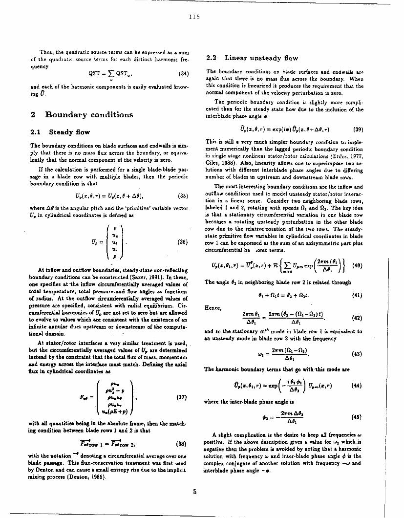
115
Thus, the quadratic source terms can be expressed as a sumof the quadratic source terms for each distinct harmonic fre- 2.2 Linear unsteady flowquency QST = QSTa, (34) The boundary conditions on blade surfaces and endwalis are
again that there is no mass flux across the boundary. Whenand each of the harmonic components is easily evaluated know- this condition is linearized it produces the requirement that theing uJ. normal component of the velocity perturbation is zero.
The periodic boundary condition is slightly more compli-cated than for the steady state flow due to the inclusion of the
2 Boundary conditions interblade phaze angle 4.
2.1 Steady flow F,(z,0,r) = exp(iO)(),(z,0+A0,r) (39)
This is still a very much simpler boundary condition to imple-The boundary condition as olad aces and bndal•ls is qiva- ment numerically than the lagged periodic boundary conditionply that there is no mass flux across the boundary, or equrva- in single stage nonlinear stator/rotor calculations (Erdos, 1977,lently that the normal component of the velocity is zero. Giles, 1988), Also, linearity allows one to superimpose two so-
If the calculation is performed for a single blade-blade pas- lutions with different interblade phase angles due to differingsage in a blade row with multiple blades, then the periodic number of blades in upstream and downstream blade rows.boundary condition is that The most interesting boundary conditions are the inflow and
UP(r, 0, r) = U,(z, 9 + Af), (35) outflow conditions used to model unsteady stator/rotor interac-tion in a linear sense. Consider two neighboring blade rows,
where AO is the angular pitch and the 'primitive' variable vector labeled I and 2, rotating with speeds flR and %l2. The key ideaU( in cylindrical coordinates is defined as is that a stationary circumferential variation in one blade row
becomes a rotating unsteady perturbation in the other bladeP row due to the relative rotation of the two rows. The steady-U( state primitive flow variables in cylindrical coordinates in bladeU, = u, (36) row I can he expressed as the sum of an &xdsymmetric part plus
u, circumferential ha tonic terms.P + {R U (Ir2 m iiz
At inflow and outflow boundaries, steady-state non-reflecting U,(z, 91, r) = (z,r)+R{EU,,exp(2 #) j (40)
boundary conditions can be constructed (Saxer, 1991). In these,one specifies at the inflow circumferentially averaged values of The angle 02 in neighboring blade row 2 is related through
total temperature, total pressure .and flow angles as functionsof radius. At the outflow circumferentially averaged values ofpressure are specified, consistent with radial equilibrium. Cir- Hence,cumferential harmonics of U, are not set to zero but are allowed 2rm 01 _ 2wm (02 - (fll - 2) t)(42)to evolve to values which are consistent with the existence of an A6, As 1infinite annular duct upstream or downstream of the computa-tional domain. and so the stationary m" mode in blade row 1 is equivalent to
an unsteady mode in blade row 2 with the frequencyAt stator/rotor interfaces a very similar treatment is used,
but the circumferentially averaged values of U, are determined 2irm (fl11 - (43)instead by the constraint that the total flux of mass, momentum " = As(and energy across the interface must match. Defining the axialflux in cylindrical coordinates as The harmonic boundary terms that go with this mode are
Pu f,( Z'63e,,, ( _ i 2 ) U,. ( x, r) (44)pU2L + p AFs puu. (37) where the inter-blade phase angle is
u.(pE+p) 46 2wsn A0 2 (4S)
with all quantities being in the absolute frame, then the match- As,ing condition between blade rows I and 2 is that A slight complication is the desire to keep all frequencies w
1'row 1 = 7row 2, (38) positive. If the above description gives a value for w2 which isnegative then the problem is avoided by noting that a harmonic
with the notation -* denoting a circumferential average over one solution with frequency w and inter-blade phase angle 0' is theblade passage. This flux-conservation treatment was first used complex conjugate of another solution with frequency -w andby Denton and can cause a small entropy rise due to the implicit interblade phase angle -0.mixing process (Denton, 1985).

116
2.3 Quadratic equations 3.2 Time-averaged total temperature varia-tions
The solid wall and periodic boundary conditions are exactly the In fans and compressors an unsteady rotor/stator interactionsame as for the steady flow analysis. The inflow and outflowboundary conditions are also similar in that the circumferen- can lead to a circumferential variation in time-averaged total
tial harmonics are again specified by steady-state non-reflecting temperature in the absolute frame. This spatial variation can
boundary condition theory. At stator/rotor interfaces, the cir- cause significant complications in the experimental determina-
cumferentially averaged values of the second order flow pertur- tion of the efficiency of the rotor. This phenomenon has been
bations are set by the requirement that the average fluxes (aver- documented and explained My in a paper by Epstein e. al
aged both in time and circumferentially) must match. Substitut- (1989). It is due to the potential field of the stator causing aning the asymptotic expansion of the flux and then time-averaging oscillation in time of the circulation around the rotor. This pro-gives the following equationo duces a shed vortex sheet which in turn, in the absolute frame ofthe stator, gives a spatial variation in total temperature which
- can be explained through the time-averaging of Crocco's theo-Fa, + c2(Fa, + Fat)row 1 = Fat + eO(F,, + Fs)row 2- (46) rem. The phenomenon is linear, with the amplitude of the total
temperature nonuniformity being proportional to the amplitudeCanceling the d (1) terms which match in the steady-state equa- of the oscillation in the rotor blade circulation.tions, yields
This phenomenon will be captured by the steady-state andlinear perturbation analysis in a three-step process. This first
Fat + Fatrow I = Fat + Fat row 2- (47) step is a steady-state combined rotor/stator computation. The
Alternatively, if one adopts the other approach to the second second step is the computation of the linear harmonic unsteadi-ness in the rotor due to the first (and possibly second) circum-order analysis by adding U to U to form the time-average U, ferential spatial harmonics in the stator inflow plane. The un-
then one obtains the matching condition steadiness in the rotor frame of reference produces downstream
2_ = propagating acoustic and vortical disturbances. A circumferen-Pat + ¢2F 2.row 1 = 7;. + 62 Fatrow 2" (48) tial Fourier decomposition shows that some of the modes are
stationary in the absolute frame of reference. These modes areIn this form, the matching condition is similar to a mathematical then input as boundary conditions for a steady linear perturba-constraint derived by Adamczyk to ensure the correct transfer tion analysis in the stator which will produce the time-averagedif time-averaged, circumferentially averaged vorticity across the spatial variation of total temperature. In this application the
interface (Adamczyk, 1991). second order quadratic effects do not play a significant role.
3 Possible Applications 3.3 Losses due to unsteadiness
The purpose of this section is to discuss the variety of different One of the most important parts of stator/rotor interaction is
phenomena which can be analyzed using the approach outlined the potential interaction, the effect of the pressure field about
in this paper. one blade row on a neighboring blade row in relative motion.The potential interaction generates acoustic waves, and withthe exception of theosituation discussed in the previous exam-
3.1 Wake and hot streak migration pIe, most of the waves are unsteady in both frames of reference.Associated with these waves is a certain level of acoustic energy,
In a compressor, rotor wakes migrate towards the pressure sur- and the question which then arises is whether this acoustic en-face of the stators downstream (Kerrebrock, 1970). Similarly, ergy is eventually dissipated (converted into thermal energy within a turbine first stage, hot streaks coming from spatial nonuni- an increase in entropy and a decrease in stagnation pressure).formtities in the combustor migrate towards the pressure surface This topic is addressed in a paper by Fritsch (1992) in whichof the rotor leading to elevated heat transfer (Butler, 1986). In it is argued that most of this energy will be lost. The physicalboth cases the mechanism is essentially the same. The unsteady m -chanism is the unsteady pressure field generating an unsteadyvelocity of the wake or hot streak relative to the mean flow drives Stokes' layer at the bottom of the boundary layer, leading to in-the fluid across the passage towards the pressure surface. The creased dissipation in the boundary layer. By contrast, an order-time-averaged effect is quadratic in the level of unsteadiness, of-magnitude analysis comes to the conclusion that in numericalFor example, the elevated surface temperature in the turbine computations the energy is lost in the freestream portion of theis proportional to both the unsteady velocity and the unsteady flow due to numerical smoothing. A supposition (possibly plau.perturbation in temperature. sible or possibly just hopeful) is that a numerical computation
Such phenomena will be captured by the second order anal- may still correctly calculate the overall additional loss providedysis using the quadratic source terms. In the case of the hot it correctly predicts the rate of generation of the acoustic energystreaks, the quadratic term in the energy flux which reflects the due to the potential interactions.qigration effect is of the form 9T. If this supposition is true, and a nonlinear, time-marching
flow calculation including numerical smoothing can indeed pre-dict the increased losses due to this form of unsteadiness, then
6
117
the full steady/linear,/quadratic analysis in this paper should be Referencesequally successful. This is a quadratic effect since the acousticenergy level is proportional to the square of the unsteady flow R. S. Abhari, G. R. Guenette, A. H. Epstein, and M. B.quantities. Giles. Comparison of time-resolved turbine rotor blade heat
If the supposition is not correct then it will be necessary to transfer measurements and numerical calculations. ASME Pa-extend the theory in this paper to an asymptotic analysis of the per 91-GT-268, June 1991.Navier-Stokes equations. It will also be necessary to use very J. J. Adamczyk. Model equations for simulating flows inmuch finer computational grids to eliminate the errors due to multistage turbomachinery. ASME Paper 85-GT-226, Junethe numerical smoothing. Of course this will greatly increase 1985.the computational cost of such calculations. J. J. Adamczyk, M. L. Celestina, T. A. Beach, and M. Bar-
nett. Simulation of three-dimensional viscous flow within a mul-tistage turbine. ASME Paper 89-GT-152, June 1989.
4 Concluding Remarks J. J. Adamczyk. A mathematical constraint placed uponinter-blade row boundary conditions used in the simulation of
This paper has presented an asymptotic approach toward the multistage turbomachinery flows. AGARD PEP 77th Sym-
calculation of unsteady flows in multistage turbomachinery. The posium on CFD Techniques for Propulsion Applicatiors, May
analysis proceeds in three phases. First one performs a steady- 1991.
state multistage analysis in which the flow is assumed to be G. K. Batchelor. An Introduction to Fluid Dynamics. Cam-
steady in each blade row in a frame of referehce rotating with the bridge University Press, 1967.
blade row. The stator/rotor interface matching conditions en- T.L. Butler, O.P. Sharma, /.D. Joslyn, and R.P. Dring.
sure overall conservation of mass momentum and energy across Redistribution of an inlet temperature distortion in an axial flow
the interface, turbine stage. AIAA Paper 86-1468, 1986.Y. S. Chen. 3-D stator-rotor interaction of the SSME.
In the second phase the unsteadiness in each blade row is AIAA Paper 88-3095, 1988.treated as a perturbation to the steady flow field. Assuming the W. N. Dawes. Towards improved throughflow capability:perturbation is small it is represented by the linearized unsteady The use of 3D viscous flow solvers in a multistage environment.flow equations. The linear stator/rotor interaction is calculated ASME Paper 90-GT-18, June 1990.by recognizing that a steady circumferential variation in a stator J. D. Denton. The calculation of 3D flow through any type
corresponds to a rotating unsteady disturbance in a rotor, and of turbomachine blade row. AGARD Lecture Series 140, 1985.vice versa. Each circumferential harmonic produces a response J. D. Denton. The calculation of three dimensional viscousof a different frequency. Due to linearity these can be com- flow through multistage turbomachines. ASME Paper 90-GT-
puted independently and superimposed to form the composite 19, June 1990.unsteady flow. D. J. Dorney, R. L. Davis, and 0. P. Sharma. Two-
The third phase calculates the change to the mean flow due dimensional inlet temperature profile attenuation in a turbineto second urder consequences of the unsteady flow field. This is stage. ASME Paper 91-GT-406, June 1991.achieved through the evaluation of quadratic source terms which A. H. Epstein, M. B. Giles, T. Shang, anO A. K. Sehra.are similar in origin to the Reynolds stress terms in the Reynolds Blade row interaction effects on compressor measurements.
averaged Navier-Stokes equations. AGARD 74th Specialists Meeting on Unsteady Aerodynamic
Through this process one can calculate the key features of Phenomena in Turbomachines, Aug 1989.
the unsteady flow in turbomachinery, the unsteady forces and J. I. Erdos, E. Alzner, and W. McNally. Numerical Solu-
moments on blades due to interactions with neighboring rows, tion of Periodic Transonic Flow Through a Fan Stage. AIAA
as well as the average effects on mass flow and efficiency. The Journal, 15(11):1559-1568, Nov 1977.
efficiency changes come about as the result of wasted kinetic en- A. Fourmaux. Unsteady flow calculation in cascades.
ergy associated with the eventual dissipation of acoustic energy ASME Paper 86-GT-178, 1986.
generated by unsteady stator/rotor interaction. A more com- G. Fritsch and M. B. Giles. Second-order effects of un-
plete treatment of efficiency prediction would require the appli- steadiness on the performance of turbomachines. Submitted to
cation of the entire asymptotic approach to the Navier-Stokes the 37th, IGTI Gas Turbine Congress, 1992.
equations. This is an algebraically complicated but otherwise M. B. Giles. Calculation of unsteady wake/rotor interac-
straightforward extension which will be tackled in the future. tion. AIAA Journal of Propulsion and Power, 4(4):356-362,July/August 1988.
This paper does not present any computational results, but M. B. Giles. Numerical methods for unsteady turbomachin-clearly this conceptual approach needs to be thoroughly vali- cry flow. VKI Lecture Series 1989-06, 1989.dated by comparison to nonlinear time-marching methods and M. B. Giles. Stator/rotor interaction in a transonic tur-experimental data. This will be addressed in future work, along bine. AIAA Journal of Propulsion and Power, 6(5), September-with the task of accelerating the numerical computations using October 1990.techniques such as multigrid. The two reasons at present to M. B. Giles and R. Haimes. Validation of a numericalbelieve that there is some merit to this idea are that Adam. method for unsteady flow calculations. ASME Paper 91-GT-czyk has already achieved significant improvements using his 271, June 1991.passage-averaged flow equations, and the alternative approach K. C. Hall. A Linearized Euler Analysis of Unsteady Flowsof nonlinear unsteady multistage calculations requires excessive in Turbo achinery. PhD thesis, M.I.T., Sept 1987.computation times.
7

118
K. C. Hall and E. F. Crawley. Calculation of unsteady qowsin turbomachinery using the linearized Euler equations. ALAJournal, 27(6):777-787, June 1989.
K. C. Hall and W. S. Clark. Prediction of unsteady aero-dynamic loads in cascades using the linearized Euler equationson deforming grids. AIAA Paper 91-3378, June 1991.
L. He and J. D. Denton. Inviscidwviscous coupled solutionfor unsteady flows through vibrating blades. Part I: Descriptionof the method. ASME Paper 91-GT-125, 1991.
H. P. Hodson. An inviscid blade-to-blade prediction of a.wake-generated unsteady flow. ASME Paper 84-GT-43, June1984.
D. G_ Holmes and H. A. Chuang. Two dimensional lin-earized harmonic Euler flow analysis for flutter and forced re-sponse. Sixth International Symposium on Unsteady Aerody-namics, Aeroacoustics and Aeroelasticity of Turbomachines andPropellers, Sept 1991.
A. B. Johnson, M. J. Rigby, M. L. G. Oldfield, and M. B.Giles. Nozzle guide vane shock wave propagation and bifurca-tion in a transonic turbine rotor. ASME Paper 90-GT-310, June1990.
J. L. Ke,'rebrock. and A. A. Mikolajczak. Intra-stator trans-port of rotor wakes and its effect on compressor performance.ASME Paper 70-GT-39, 1970.
T. Korakianitis. On the propagation of viscous wakes andpotential flow in axial turbine cascades. ASME Paper 91-GT-373, June 1991.
D. R. Lindquist and M. B. Giles. On the validity of fin-earnzed, unsteady Euder equations with shock capturing. AIAAPaper 91-1958, 1991.
R. A. Kulawc and J3. 3.Adarnczyk. The numericai simulationof .high-speed axialflow compressor. ASME Paper91-GT-272,June 1991.
R&-H. Ni and. F. Sisto. Numerical computation of nonsta-tionaty aerodynamics of tat plate cascades in compressible flow..ASMELPaper-75-GT-5, 1975.
J.- Paidon, Z.. Zhang, P. Jia, and J. Meng. Influence of un-steady effects on the measurements in a transonic axial com-pressor. ASME Paper 91-GT-90, 1991.
M.- M. Rai. Navier-Stokes simulations of rotor-stator in-teraction using patched and overlaid grids. AIAA Journal ofPropulsion and Power, 3(5):387-396, 1987.
M.M. RaL Three-dimensional Navier-Stokes simulations ofturbine, rotor-stator interaction. AIAA Journal of Propulsionand Power,, 5(3):305-319, May-June 1989.
A. A. Rangwalls, N.K. Madavan, and P. D. Johnson. Appli-cation of an unsteady Navier-Stokes solver to transonic turbinedesign. AIAA Paper-91-2468, 1991.
A.. Saxer and W. Giles. Quasi-3D nonreflecting boundaryconditions for Euler equation calculations. AIAA Paper-91-1603,June 1991.
H. Schlichting.. BounSary Layer Theory. McGraw-Hill,1979.
L. D. Siden. Numerical simulation of unsteady viscous com-pressible flows applied to blade flutter analysis. ASME Pal -r914GT-203, 1988.
A. Suddhoo, M. Giles, and P. Stow. Simulation of inviscidblade row interaction using a linear and a non-linear method.ISABE Conference, 1991.
8
119
TASK III: UNSTEADY PHENOMENA AND FLOWFIELD INSTABILITIES
IN MULTISTAGE AXIAL COMPRESSORS
(Investigators: E.M. Greitzer, C.S. Tan, P.P. Silkowski, J.P. Longley,N.A. Cumpsty, I.J. Day, D.C. Wisler, H.W. Shin)
Executive Summary
This progress report describes a combined experimental and theoretical program of
research on unsteady flow and instability in multistage axial compressors. The objectives of the
program were to define the critical fluid dynamic phenomena associated with the onset of
instability in modem, multistage machines and assess those elements that should be incorporated
in improved models of this process. The specific research goals included elucidation of newly
discovered types of propagating disturbances, having widely disparate wavelengths and waves
speeds, which occur prior to rotating stall onset, and definition of the extent to which current
unsteady flow models capture the relevant fluid processes of this complex dynamical system. The
work is being carried out in collaboration with the General Electric Aircraft Engine Company, with
the experiments actually being conducted at the GE Aerodynamics Research Laboratory, on a
facility representative of advanced aeroengine compressor geometries.
Two main activities are discussed in the report. The first is unsteady measurements of the
blade passage flo, v field in the first rotor of a multistage compressor, under conditions at which
stall occurred naturally as well as under conditions in which the flow was artificially stabilized, so
that the behavior at, and even past, the nominal stall point could be addressed. This gives new
information concerning the interaction and role of the different wavelength unsteady disturbances.
The second is a series of diagnostic experiments with a forced unsteady inlet distortion, which
allowed detailed assessment of the concepts that underlie the existing wave dynamic models of
compressor response to inlet non-uniformity.

120
I1.0 nltrodulction
Recent studies of rotating stall irception have led to the definition of two different paths
from the essentially axisymmetric flow in the pre-stall state to fully developed rotating stall. The
first involves the growth of a small amplitude, long circumferential length scale (of the order of the
machine radius) traveling wave into a fully developed rotating stall cell. The initial propagation
speed of the traveling wave is close to that of the developed stall cell, and small amplitude traveling
waves can exist for a long time (several tens of rotor revolutions) before any operational changes
in machine behavior occur. This process is well captured by the models of unsteady flow in
multistage machines.
Another, quite different, process has also been observed, however, which involves the
circumferential growth of a small circumferential extent disturbance (a few blade pitches) into a
mature rotating stall cell in roughly five to ten rotor revolutions. These small extent, or short
length scale, phenomena will be referred to here as spikes, primarily because their temporal history
appears considerably more "spiky" than the long length scale disturbances. An important factor in
the design of the experiments to be discussed was the desire to focus on the different time and
length scales associated with the spikes and the long wave disturbances (referred to as LWD's). In
particular, the axial locations of probes upstream of the rotor were intended to spatially filter out
short length scale disturbances and make the long wavelength disturbances clearer. Also, several
rig modifications were used as tools to focus on specific time and length scales, including
restaggering the rear three stages, asymmetric tip clearance, and distortion screens.
The basic fluid dynamic questions that were initially addressed in this study were:
1) What are the mechanisms of rotating stall inception?
2) Is there a repeatable pre-stall event, and if so, is it a long wavelength disturbance (LWD), a
short wavelength disturbance (spike), or some combination of the two?
3) Can one associate the type of pre-stall events with compressor design parameters?
4) At the blade passage length scale how do the various fluid dynamic structures (tip

121
vortex/leakage jet, blade wakes, and endwall boundary layers) behave with changing operating
point and what role do these structures play in the stall inception process?
5) How do inlet distortion and changes in tip clearance affect the stall inception process?
6) If we are able to artificially stabilize the first stall flow, what is the axisymmetric machine and
local flow field behavior in the first stage at these highly loaded conditions, i.e. what, in detail,
is the flow field associated with "compressor stall"?
To address these questions, an investigation of a multi-stage compressor flowfield has
been conducted involving several different levels of experimentation. Detailed examination of the
first stage rotor has been carried out during a series of experiments in which the flow was
artificially stabilized by restaggering the rear three stages. This restaggering created a situation in
which the behavior of the rear three stages suppressed the growth of long length scale flow
disturbances. This enabled the behavior of the first rotor, at flows below that where the rotor
would experience stall in a natural environment' to be seen. As will be described, the experiments
show that although the stall inception process may begin as a localized event, the evolution into
rotating stall is governed by the environment defined by the coupling of the various compression
system components. Also, the rotor tip leakage jet appears to be a key feature in the local stall
inception process.
As a second facet of the program, diagnostic experiments have been carried out to examine
the effect of unsteady inlet distortions on instability onset, i.e. to address the issue of the receptivity
of the compressor, considered as a multi-dimensional dynamic system, to inlet disturbances. This
set of experiments also allows assessment of wave models of unsteady compressor response that
have been developed.
The first experiments showed clearly, perhaps for the first time, that the path to stall can
involve the interaction of disturbances of both long and short wavelength perturbations.
Understanding the connection between these types of disturbances is a critical new conceptual step
in attacking this important problem.

122
2.0 Experimental Facilities
The investigation included theoretical and experimental phases and was a collaborative
university-industry effort, involving groups at MIT and General Electric Aircraft Engines. There
was also participation from the Whittle Lab, Cambridge, England. The experiments were carried
out at the General Electric Aerodynamics Research Laboratory, under the aegis of Dr. D.C.
Wisler. The facility used was a large scale, low speed research compressor that presents a model
of many aspects of the actual high speed compressor flow field (Fig. 1). The large size minimizes
probe blockage and allows for easier access and instrumentation whilst giving correct Reynolds
number at low operating speed. A four-stage compressor was used with the NASA/GE Energy
Efficient Engine blading. Further information on this facility and the blading can be obtained from
Ref [1].
In addition to standard steady state instrumentation, high response pressure transducers and
hot wires were used. A radially traversable slant wire, to give three components of velocity, and a
total pressure probe were also used at rotor inlet and rotor exit. The bulk of the experiments were
carried out with fixed arrays of 40 probes, consisting of 20 hot wires and 20 pressure transducers.
At inlet guide vane exit, there were ten reference hot wires at midspan and ten corresponding
pressure transducers in the casing. The ten reference locations were circumferentially distributed at
eight equally spaced locations to facilitate spatial Fourier analysis. Two closely spaced sensors
were also used to allow cross-correlations over various distances, to combat spatial aliasing. Most
of the unsteady data was sampled at 10 kHz and low pass filtered at 3 kHz, with several cases
sampled at 1 kHz and low pass filtered at 300 Hz.
Complementing the reference probes were ten additional hot wires and ten casing pressure
transducers with circumferential distribution identical to the reference probes referred to above.
The reference probes were fixed at their locations for all runs as a control, but the test probes were
moved to various axial-radial positions. The test probes were used at four axial locations: one half
of a radius and one quarter of a radius upstream of rotor inlet, one at rotor inlet, and one at rotor
exit, at locations roughly 0.2 chord upstream and downstream of the rotor respectively. At R/2 or
123
R/4 upstream, the hot wires were at midspan, but at rotor inlet and rotor exit, the hot wires were
used at 20% and 80% immersion (tip and hub), as well as at other immersions, as shown in Fig.
2. To focus on small length scale events, experiments were also performed with eight probes
equally spaced over three blade pitches.
The baseline build overall compressor characteristic (pressure rise versus axial velocity
parameter at constant rotor speed) is displayed in Fig. 3. Figure 4 is the performance of the first
stage only. Several points are labeled for future reference. Point A is design and point E is just
before rotating stall occurs.
For the restagger, the rear three rotors were closed by 100. Figure 5 shu vs the result of the
restagger on the overall pressure rise characteristic. The stalling flow coefficient was changed
from 0.345 to 0.308. Thus, the purpose of the restagger, which was to extend the stable operating
region of the first stage and provide a clearer view of the spikes by suppressing the long length
scale disturbances, has been achieved. There is an abrupt change in slope of the overall
mismatched characteristic at the stalling ý of the baseline build.
Figure 6 displays the first stage characteristic for the baseline and restaggered builds with
several operating points labeled for future reference. In the range of flows common to the two
builds, the first stage pressure rise characteristic is the same for both. The extended operating
region of the first stage characteristic (achieved with the restagger), however, is positively sloped.
Stability analysis predicts that a positively sloped compressor stage would exhibit flow instability;
here the rear three stages are negatively sloped and the QovralH compressor has a negative slope and
hence is stable.
A second variation from the baseline build was to open the first stage rotor clearance from
gap/span = 1.3% to 3.1%. This was done both symmetrically as well as by opening the clearance
over a 1200 section of the annulus.
124
3.0 BReuts
3.1 Steady State Blade Row Flow Field Data
The steady state blade row data are presented in two ways: radial profiles, i.e. mass
averages over one circumferential pitch at a given radius, and contour or vector format over
roughly 1.5 blade pitches.
Figure 7 shows the radial velocity distribution at inlet to the first rotor at various operating
points. This should be close to zero if the flow is unstalled. Although the flow angles in the tip
region for the extended operating region of the restaggered build were out of calibration range for
the slant wire, useful information can still be obtained from the data. In particular, the plot shows
that the tip flow field does not deviate from the expected direction until operating point J of the
restagger build, which is the baseline stalling flow coefficient. As the flow coefficient decreases
further, an increasingly large portion of the tip flow field is out of range for the slant wire.
( Figure 8 is a display of the slant wire data at rotor exit at the stable operating point closest
to stall in the baseline build. The data has been converted to the relative (rotor) frame and is
viewed at a yaw angle of 550 from axial, i.e. an angle aligned with the bulk through flow direction,
so the figure represents the cross-plane or secondary flow. The scale vector at the top shows the
direction of rotor rotation and the magnitude of blade tip speed, Utip. Blade wakes, which have
strong radial transport, and the tip vortex/leakage jet flow is clearly visible.
Figures 9 and 10 show the throughflow velocity at different flow coefficients with the
contour of velocity/Utip < 0.45 shaded. A change in the tip region between points D and K is
seen; there appears to be an almost axisymmetric region of low velocity near the tip at point IL
Figure 11 shows the axial velocity distribution at 50% immersion (mid-span) at rotor exit for
roughly 1.5 pitch at three diiferent flow coefficients, and it is seen that the rotor wakes do not grow
much circumferentially in 0 as ý decreases. Figure 12 displays axial velocity profiles for two
operating points at rotor exit for the baseline and for a larger first stage tip clearance. An increase
of axial flow deficit can be seen near the tip with the larger clearance.
To summarize the steady state data, as the flow (0) decreases the tip vortex/jet structure

125
and the rotor wakes do not change qualitatively, but close to stall the rotor leakage jet becomes
larger. Furthermore, for the restaggered case, starting at the baseline stall flow coefficient, a region
of appreciable radial velocity at rotor inlet grows in radial extent with decreasing flow coefficient.
Finally, although the data is not shown here, the larger tip clearance build had a larger axial velocity
deficit in the tip region, than the baseline build.
4.0 Time-Resolved Data
4.1 ine Build
Figure 13 shows time traces for eight equally-spaced casing pressure transducers at rotor
inlet. Probe numbers increase in the direction of increasing 0 in the rotor rotation direction, and
time is in units of rotor revolutions. The figure displays a situation in which the compressor was
set at a stable operating point close to stall and the throttle slowly closed until the machine went
into stall. A spike is first visible at t - 76.5 on pressure transducer number 5. The growth of the
spike, in amplitude and circumferential extent, is seen over the next few rotor revolutions, resulting
in a developed stall cell by t - 82. There are no apparent propagating disturbances prior to time -
76.5.
Guidelines have been drawn in Fig. 14, with the slope of these lines representing the speed
of propagation of the disturbance around the annulus. The change in slope of these lines indicates
the change in the speed of propagation of the disturbance as it decelerates from 70% at inception to
45% as a mature stall cell. No evidence of any long wavelength disturbances above the
perturbation levels of (permt tion velocity)/U = 0.5%, p'/pU2 = 1% could be found. The data
analysis techniques used confirmed the spike's 70% initial speed and subsequent deceleration to
45% with growth in magnitude and circumferential extent.
An example of the data analysis technique used is shown in Fig. 15. At each discrete time,
data from eight equally spaced probes were Fourier analyzed and the resulting magnitudes and
phases for the various harmonics displayed. The size of the symbols are scaled by the amplitude
of the disturbance. No propagating disturbances are visible prior to time = 77, at which point the

126
disturbance grows rapidly to final size within roughly five rotor revolutions. The continuous
change in slope of the phase of the first Fourier harmonic indicates the deceleration of the spike.
(The regular pattern seen for times prior to t - 77 in harmonic one is attributed to a slight rotor
geometry asymmetry.)
Some experiments were conducted with the eight equally spaced test wires alternating
between hub and tip, 80% and 20% immersion. Figure 16 displays the results from one of these
tests conducted at rotor inlet, which shows the three-dimensional nature of the spike. Between t -7
7 and t - 78, the spike is seen as an axial deficit traveling in the tip region, with no disturbance
visible in the hub wires. Only after the tip deficit has grown appreciably is any disturbance visible
at the hub at t - 78.5. The hub disturbance is first seen as a flow increase (partially compensating
for the tip blockage), but as the spike grows into a stall cell, a full span deficit eventually occurs.
Time-resolved measurements thus show the baseline build stalled via radial and
circumferential growth of an initially small length scale disturbance. The growth occurred in
roughly five rotor revolutions and no modal signals were found. The disturbance initial speed of
70% decreased to 45% as it grew into a mature stall cell.
5.0 R aered Build
As the throttle was closed for the mismatched build, the following sequence of events
occurred. When the flow coefficient decreased to the level at which the baseline encountered
rotating stall, spikes would appear and disappear. As the flow was decreased further, to J, more
spikes would appear per unit time with the spike width increasing from roughly 2-3 blade pitches
to 3-4 blade pitches.
As the flow coefficient was decreased from J, the spike disturbances became more regular,
they did not decay after a short appearance, but persisted. Time traces, FFTs, and correlations all
showed this. The disturbances traveled at roughly 70%. At operating point N, there were 12
spikes traveling about the annulus at 70%. For any further decrease in flow, one of these would
grow into rotating stall in the same fashion as the baseline case. As in the baseline case, the spike

127
disturbance gives an initial tip axial velocity deficit and a hub velocity increase until the disturbance
evolves to cover the full span. The spike disturbance circumferential size at the hub is on the order
of one or two pitches.
The disturbances with the restaggered build have similar features to the spike transients for
the baseline build. Both appear first at operating point J and travel at a speed of roughly 70%.
Both have a radial velocity distribution with a tip deficit and a hub increment in flow. The
circumferential size (few pitches) of the disturbances of the restaggered build is comparable to that
with the baseline build, early in its growth. The stabilized disturbance with the restaggered build
thus resembles the spikes of the baseline build at some time during the five rotor revolution
growth period of the latter. It therefore appears that the stabilized disturbances of the restaggered
build and the transient disturbance of the baseline build may be the same phenomena, although this
has not been proven conclusively. This is important because it suggests that one can use
restaggering to enable more accurate flow diagnosis of these events.
6.0 Response of Multistage Comnressors to Rotating Inlet Flow Distortions
The second main thrust in this task has been the assessment of the effect of unsteady inlet
disturbances on multistage compressor performance and stability. The motivation for the work
arises out of two compelling factors concerning operability of gas turbine engines. First is that
stability limitations often arise not with uniform flow, but as a result of an inlet non-uniformity, or
distortion. Further, distortions encountered in practice usually have significant asymmetry to
them, so that the problem of compressor response to circumferential inlet distortion is a real one
indeed.
The second aspect is that the instability process is an inherently unsteady one, and the
behavior of multistage machines, considered as dynamic systems, is not well understood. The
consequence is that it is not scientifically correct to break up the response into smaller, much
simpler modules, and study each one separately in the hope that one can somehow learn about the
overall behavior. To do so is to ignore the real issues of the dynamic coupling between blade

123
passages, blade rows, and compressor stages which give rise to the response of interest.
These background facts led us to the set of experiments to be described, which made use of
a rotating screen to create an unsteady inlet non-uniformity, which served as a unique diagnostic
tool. Although the use of the rotating screen arose primarily for this reason, it can be mentioned
that circumferential non-uniformities which can rotate at fixed speed around the compressor
annulus can occur in two-spool compression systems, where one of the compressors or the fan
could be in rotating stall, subjecting the other to a non-uniform rotating flow pattern.
There is little detailed data concerning the behavior of compressors when subjected to such
types of distortions, but experimental results [2], [3] suggest that disturbances which rotate at
speeds similar to stall ceU propagation speed have the most pronounced effect. This behavior can
also be seen in the computations of [4] which linked the phenomena to the resonant response of
the compressor, i.e. to a correspondence between the forcing and the natural eigenmodes of the
( compression system.
The investigation of the effect of rotating flow non-uniformities on multistage compressor
performance described here had three central objectives: to obtain information on the overall
behavior (surge line changes) as a function of distortion rotation speed; to characterize the unsteady
response of the compressor, and to assess present theoretical approaches to compressor stability.
The last is particularly important since the existing models make use of rudimentary descriptions
of the unsteady flow in the compressor blades, and it is not known to what extent this affects the
predictions of overall behavior.
For the present experiments, the General Electric large scale research compressor described
earlier was equipped with a drive mechanism which could rotate a distortion screen at speeds
between ±100% rotor speed [5]. The advantage of a screen-generated rotating distortion, rather
than one generated by another compressor in rotating stall, is that it allows independent control of
the severity of the non-uniformity, the rotation direction and speed and the compressor operating
point. The screen was located 1.5 radii upstream of the inlet guide vanes and produced a roughly
square wave stagnation pressure distortion of 1200 circumferential extent with amplitude

129
corresponding to 1.2 x [1/2 p(Cxmean) 21. This non-uniformity was chosen to give a large change in
the compressor stall point with no rotation, based upon predictions of the theoretical model.
Time mean and fast response instrumentation were used to measure the mean overall static
pressure rise of the compressor, the unsteady static pressure distribution (both upstream and
downstream of the compressor) and the time varying velocity field at various locations. These
measurements were processed to analyze both the steady flow redistribution, as seen in the frame
of reference of the distortion screen, and the behavior of perturbations which were unsteady in this
coordinate system.
In what follows, we shall present the experimental results in close conjunction with theory;
this will serve to address the capabilities of the flow models that have been developed.
7.0 Theor
The theoretical model used for the predictions and the design of the experiment was an
extension of that reported in [4], [6], and [7]. It is a general fluid dynamic stability analysis for the
compressor and the associated flowfields. The compressor performance is specified by an
axisymmetric pressure rise characteristic with a correction for non-steady effects based on a simple
model for the inertia of the fluid within the blade passages. The theory is well documented in [4],
[6], and [7], so only the changes necessary for this investigation are commented upon.
For the present situation, the mean (background) flow equations were solved in a
coordinate system rotating with the inlet distortion, so the flowfield redistribution may be
considered as time invariant. In the engine frame, however, the potential field which causes the
upstream redistribution is unsteady, and the stagnation pressure of a fluid particle is not conserved
even for an inviscid flow. This introduces an additional term into the equations, but solution of the
mean flow can be caried out in the same manner. Once the flow redistribution has been calculated
(in the rotating coordinates), the stability of the flowfield is assessed, as in the original form of the
theory, by calculation of the growth rates associated with general unsteady perturbations.

130)
8.0 Experimental Results and Comparison With Theory
The behavior of the small-amplitude perturbations, which is important in determining the
stability of the non-uniform compressor flowfield, is set by the background flow, which is a
measure of the compressor's response to the imposed inlet distortion. The theory shows that the
velocity field near stall is primarily determined by unsteady flow effects and that these change
significantly as the rotation speed of the distortion varies. A study of how screen rotation rate
affects the stability boundary of the compression system is thus useful in assessing the importance
of the unsteady fluid dynamics and the degree to which the modelling is correct.
Figures 17 through 20 show overall effects of propagation speed of the inlet distortion
(rotation rate of the screen) on the onset of flow instability in the multistage compressor. The
horizontal axis in the figure is the non-dimensional rotation rate, rotation speed divided by rotor
rotation, and the vertical axis is the value of flow coefficient, Cx/U, at which the instability, i.e.
"stall", is encountered. A higher value of this quantity means a decreased stable flow range; the
compressor stalls at a higher flow. In the figures, the experimental data are shown by the solid
lines, and the calculations by the symbols. There is more than one line in some of the figures
because there was a limitation on the mechanical speed of the screen. Data were thus taken at
several rotor RPM in order to be able to achieve a higher non-dimensional value of this quantity.
Figure 17a shows the compressor tested by Plumley, as described in [8], while Figure 17b
presents this information in more operational terms. In either of the figures, it is seen that counter-
rotation has a markedly less severe effect on compressor instability. What is of more interest is
the effect on stall margin, for example as measured by the distance between design flow and stall
flow. Figure 17b shows that a steady inlet distortion decreases this margin by about twenty-five
percent from the uniform flow value. With the rotating distortion, however, this decrease is more
than doubled, and the margin decreases to roughly one-third of the uniform flow value.
A somewhat over-simplified explanation for the decrease is that, for the rotation rates at
which the large effects are seen, the system is being subjected to disturbances that have a temporal
and spatial structure similar to its natural eigenmodes. Because of this "resonance", in the mean
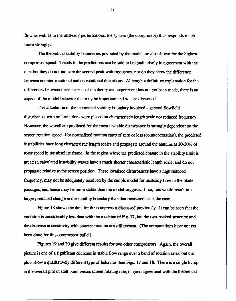
131
flow as well as in the unsteady perturbations, the system (the compressor) thus responds much
more strongly.
The theoretical stability boundaries predicted by the model are also shown for the highest
compressor speed. Trends in the predictions can be said to be qualitatively in agreement with the
data but they do not indicate the second peak with frequency, nor do they show the difference
between counter-rotational and co-rotational distortions. Although a definitive explanation for the
differences between these aspects of the theory and exper;'nent has not yet been made, there is an
aspect of the model behavior that may be important and w- be discussed.
The calculation of the theoretical stability boundary involved a general flowfield
disturbance, with no limitations were placed on characteristic length scale nor reduced frequency.
However, the waveform predicted for the most unstable disturbance is strongly dependent on the
screen rotation speed. For normalized rotation rates of zero or less (counter-rotation), the predicted
instabilities have long characteristic length scales and propagate around the annulus at 20-30% of
rotor speed in the absolute frame. In the region where the predicted change in the stability limit is
greatest, calculated instability waves have a much shorter characteristic length scale, and do not
propagate relative to the screen position. These localized disturbances have a high reduced
frequency, may not be adequately resolved by the simple model for unsteady flow in the blade
passages, and hence may be more stable than the model suggests. If so, this would result in a
larger predicted change in the stability boundary than that measured, as is the case.
Figure 18 shows the data for the compressor discussed previously. It can be seen that the
variation is considerably less than with the machine of Fig. 17, but the two-peaked structure and
the decrease in sensitivity with counter-rotation are still present. (The computations have not yet
been done for this compressor build.)
Figures 19 and 20 give different results for two other compressors. Again, the overall
picture is one of a significant decrease in stable flow range over a band of rotation rates, but the
plots show a qualitatively different type of behavior than Figs. 17 and 18. There is a single hump
in the overall plot of stall point versus screen rotating rate, in good agreement with the theoretical
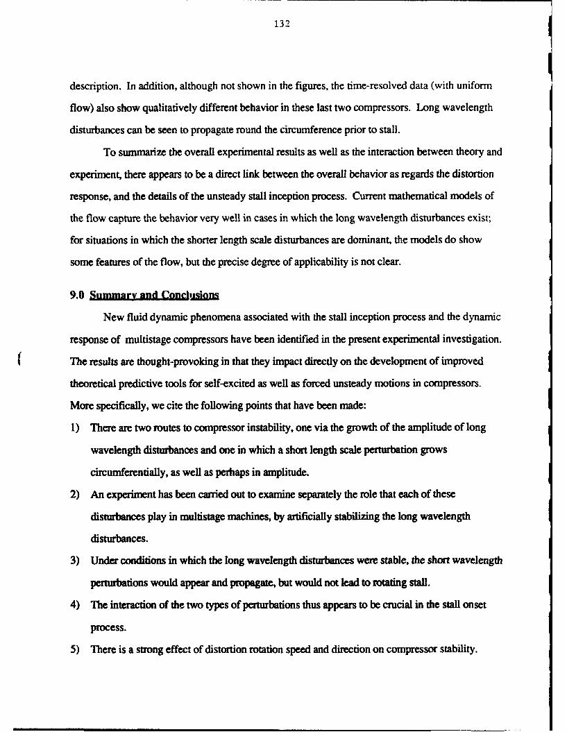
132
description. In addition, although not shown in the figures, the time-resolved data (with uniform
flow) also show qualitatively different behavior in these last two compressors. Long wavelength
disturbances can be seen to propagate round the circumference prior to stall.
To summarize the overall experimental results as well as the interaction between theory and
experiment, there appears to be a direct link between the overall behavior as regards the distortion
response, and the details of the unsteady stall inception process. Current mathematical models of
the flow capture the behavior very well in cases in which the long wavelength disturbances exist;
for situations in which the shorter length scale disturbances are dominant, the models do show
some features of the flow, but the precise degree of applicability is not clear.
9.0 Summary and Conclusions
New fluid dynamic phenomena associated with the stall inception process and the dynamic
response of multistage compressors have been identified in the present experimental investigation.
The results are thought-provoking in that they impact directly on the development of improved
theoretical predictive tools for self-excited as well as forced unsteady motions in compressors.
More specifically, we cite the following points that have been made:
1) There are two routes to compressor instability, one via the growth of the amplitude of long
wavelength disturbances and one in which a short length scale perturbation grows
circunmferentially, as well as perhaps in amplitude.
2) An experiment has been carried out to examine separately the role that each of these
disturbances play in multistage machines, by artificially stabilizing the long wavelength
disturbances.
3) Under conditions in which the long wavelength disturbances were stable, the short wavelength
perturbations would appear and propagate, but would not lead to rotating stall.
4) The interaction of the two types of perturbations thus appears to be crucial in the stall onset
process.
5) There is a strong effect of distortion rotation speed and direction on compressor stability.

133
6) A simple theoretical model of unsteady compressor response to rotating distortions shows
predictions that are qualitatively similar to the experimental results, for several compressors
and quantitatively similar for others. the difference between the two classes appears to be the
existence of small amplitude, long wavelength disturbances prior to instability.
7) Both the detailed roto, passage results and the information with the rotating inlet distortion
point to study of the fluid dynamics of the short wavelength disturbances, both structure and
evolution, as an item of extremely high priority for unsteady flows in multistage compressors.
10.0 References
1. Wisler, D.C., "Loss Reduction in Axial-Flow Compressors Through Low-Speed ModelTesting," ASME Paper 84-GT- 184, 1984.
2. Ludwig, G.R., Nenni, J.P. and Arendt, R.H., "Investigation of Rotating Stall in Axial FlowCompressors and the Development of a Prototype Stall Control System", Technical ReportUSAF-APL-TR-73-45, 1973.
3. Kozarev, L.A. and Federov, R.M., "Aspects of the Appearance and Elimination ofBreakdown in an Axial-Flow Compressor in the Presence of a Rotating Non-Uniformity atthe Inlet", Jzevstinya vuz Aviatsionnaya Tekhnika, Vol. 26, No. 1, pp. 33-37 (translated),1983.
4. Chue, R., Hynes, T.P., Greitzer, E.M., Tan, C.S. and Longley, J.P., "Calculations of InletDistortion Induced Compressor Flowfield Instability", Int. J. Heat and Fluid Flow, Vol. 10,No. 3, Sept. 1989.
5. Greitzer, E.M., Epstein, A.H., Giles, M.B., McCune, J.E., Tan, C.S., Annual TechnicalReport on Grant AFOSR-90-0035, "Unsteady Flow Phenomena in Turbomachines,"December 1991.
6. Hynes, T.P. and Greitzer, E.M., "A Method for Assessing Effects of Inlet Flow Distortion onCompressor Stability", ASME J. Turbomachinery, Vol. 109, pp 371-379, 1987.
7. Longley, J.P., "Measured and Predicted Effects of Inlet Distortion on Axial Compressors",ASME Paper 90-GT-214, Presented at the Gas Turbine and Aeroengine Congress andExposition, Brussels, Belgium, June 11-14, 1990.
8. Plumley, R.E., "Unsteady Compressor Distortion Response and Compressor Instability,"M.S. Thesis, Department of Aeronautics and Astronautics, MIT, 1990.

134
Plane 0.1 Bellmouth FlowMeasurement Plane
Plane 0.5 IGV Inlet
Plane 1.0 Rotor 1 Inlet
Plane 1.5 Rotor 1 Exit
Laboratory Floor
• Throttle
Fig. 1: Cross-section of low speed GE research compressor in0.7 radius ratio configuration.

135
lb
II
a:
CLC
• 0
• m,C
0)_
Ct

136
U')
CC
Cl
0>
C -4
m 0u
V -4
V, L 0*ý *0 9* vj'
an Id V

137
I',
00
000
0 IIn
OLI c9 TO 9
and/"y -i
Id In
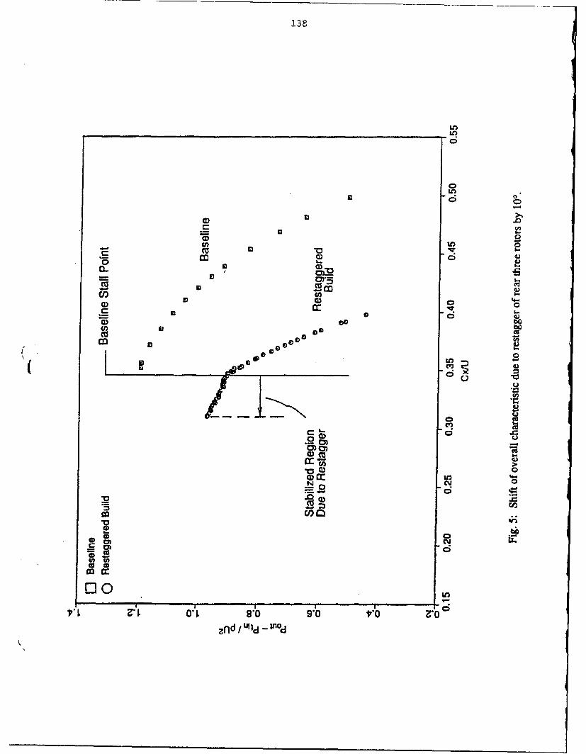
138
Cf)
0 m (0
cm-4
U)) -
-D 0 0
0) IDO
0 I
CI) aC0) .70)
CD 0Lo
0 C00
( CD
C tmc;U
im X)
OoU
0' L9*0 ,0 PO 0
znd Ull - Cn,

139
.o'00
0,
EJOto
v ci
idiC4
9L6 ) :' jo;OV So
Ucan ,Id-n

140
U) CD
imMc ci
CV,
0-Ma-
N~dS%
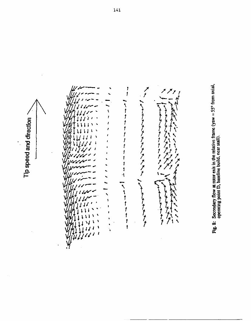
141
i 7/,,- 7
II
<.2 . y 7t Y.
""" 44 t /o'CD) " I /' t .•
I- i*1' t rS!•,• • , .
•%X

142
o • 0 0 0 0 0 0 0 1_ O 0 o LO 0D w00 ID 0
Ci 6i 6 LO o w
• O.+ X . + V N
E
0
W)
7Elu-
40) bo
&g

143
o0 C> 0 CD 0 CD 0ý C
oL 0 6 n 6 Lo 0 6 n Q m
ElE -0 + X + X< N
0
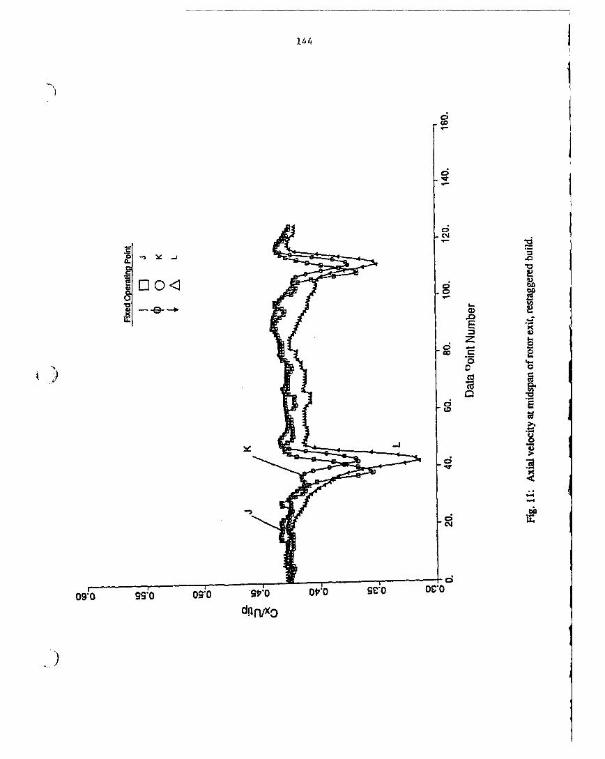
144
CD0
N
CL
oo -,
0.0
0909 .0 090'*00" v V
dilr~x
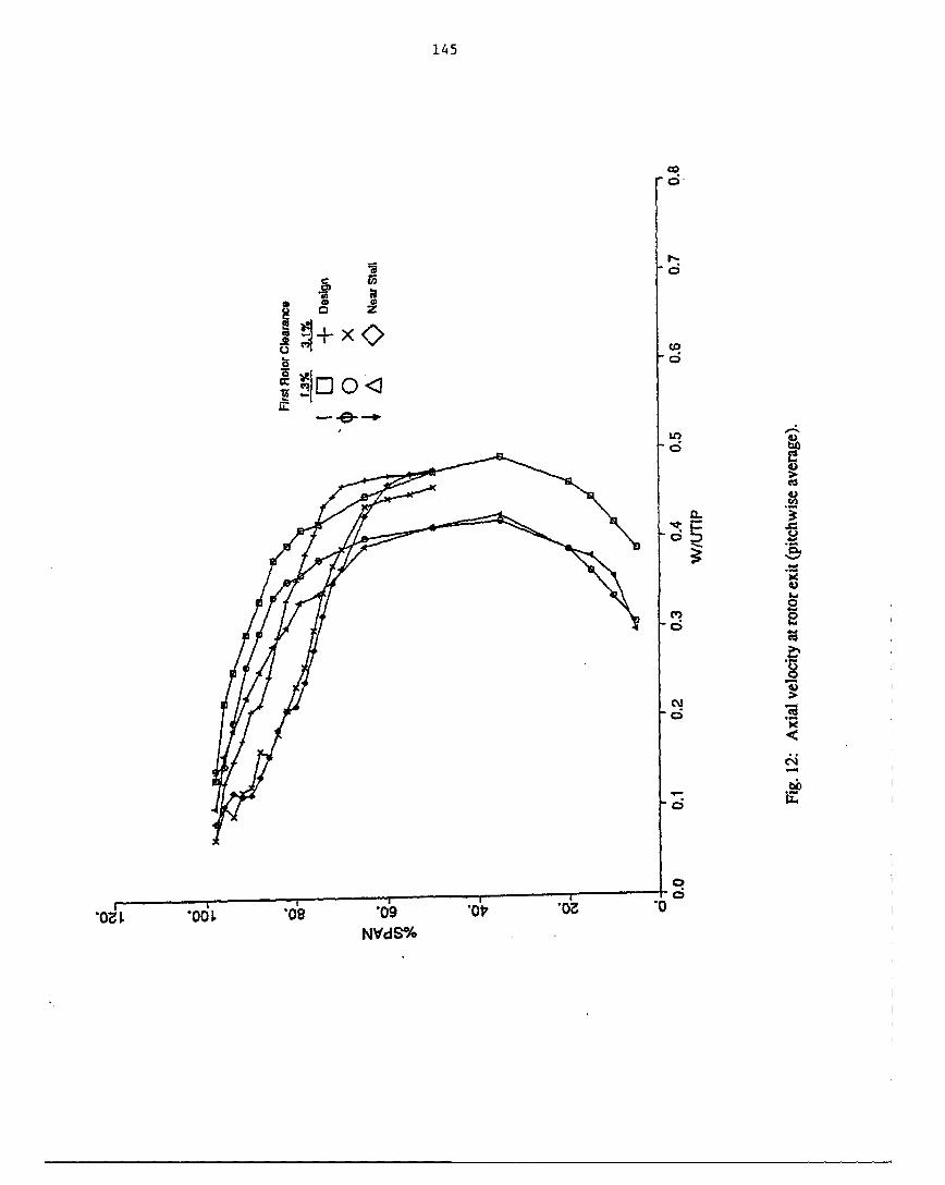
145
0*
cV.
CC
loz L *00 09 *0 *-i
N6d*0

146
gI
Go
>
I.4
w
0800
-- uo42108 JOlou
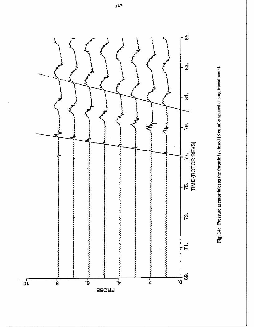
147:
u-i
00
U)U
00F-
w
3901d0
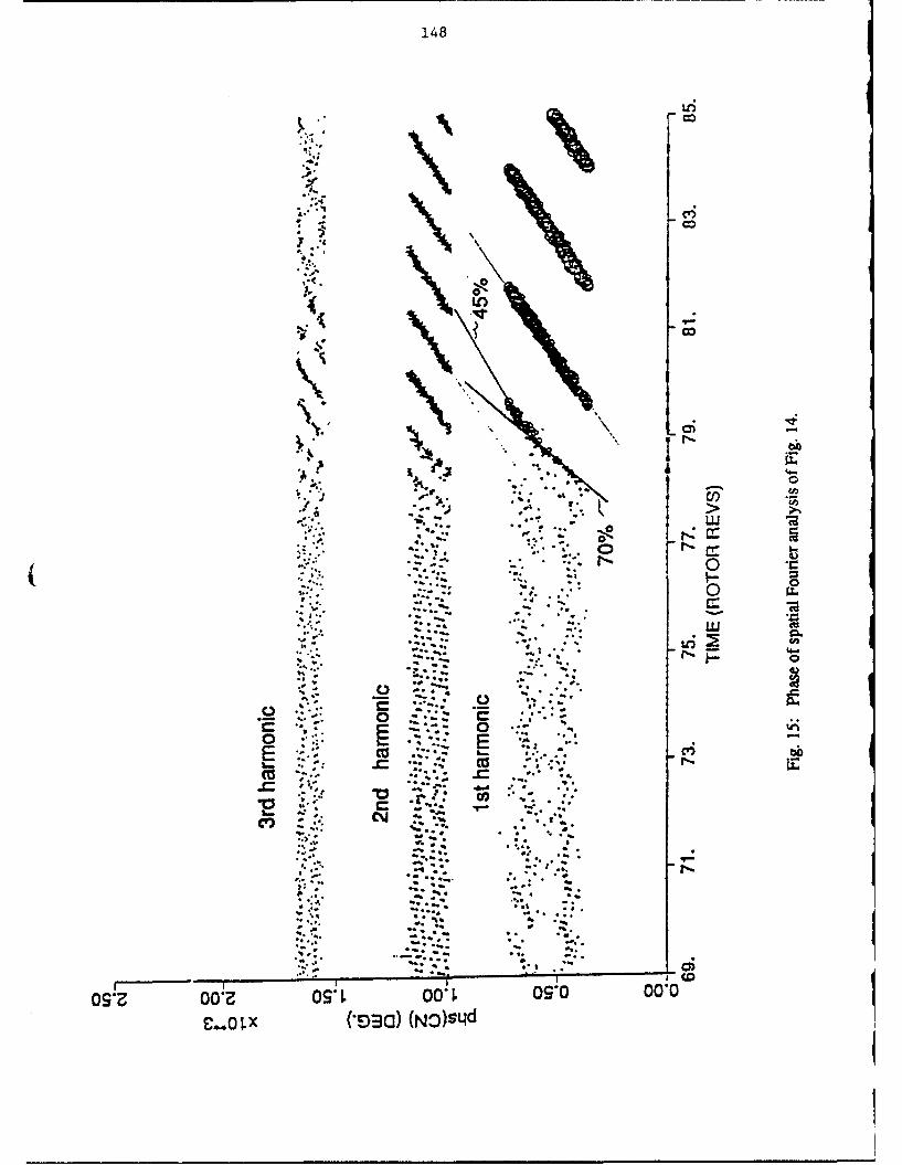
148
L6
C6-. 5.o
a00
C) I=5
a as
09 007. ..* 09* T
S'.V -*)0 -.~si
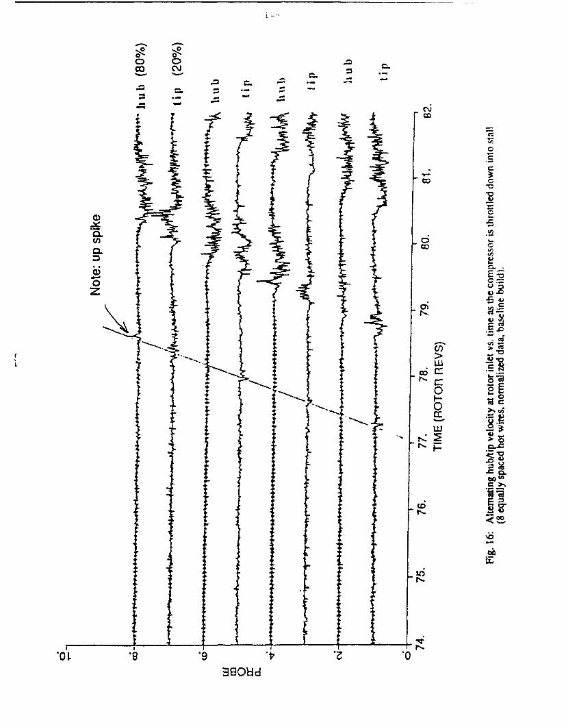
o 0 -
OD~ C.j
CL.
00
I cII V
zr
*OL .8 .9 *
-'---9908

150
toAa 0E
C6
00
A cu
0 CD
0 0
x ~0
w U)
0 00 )
aul leEG3490M
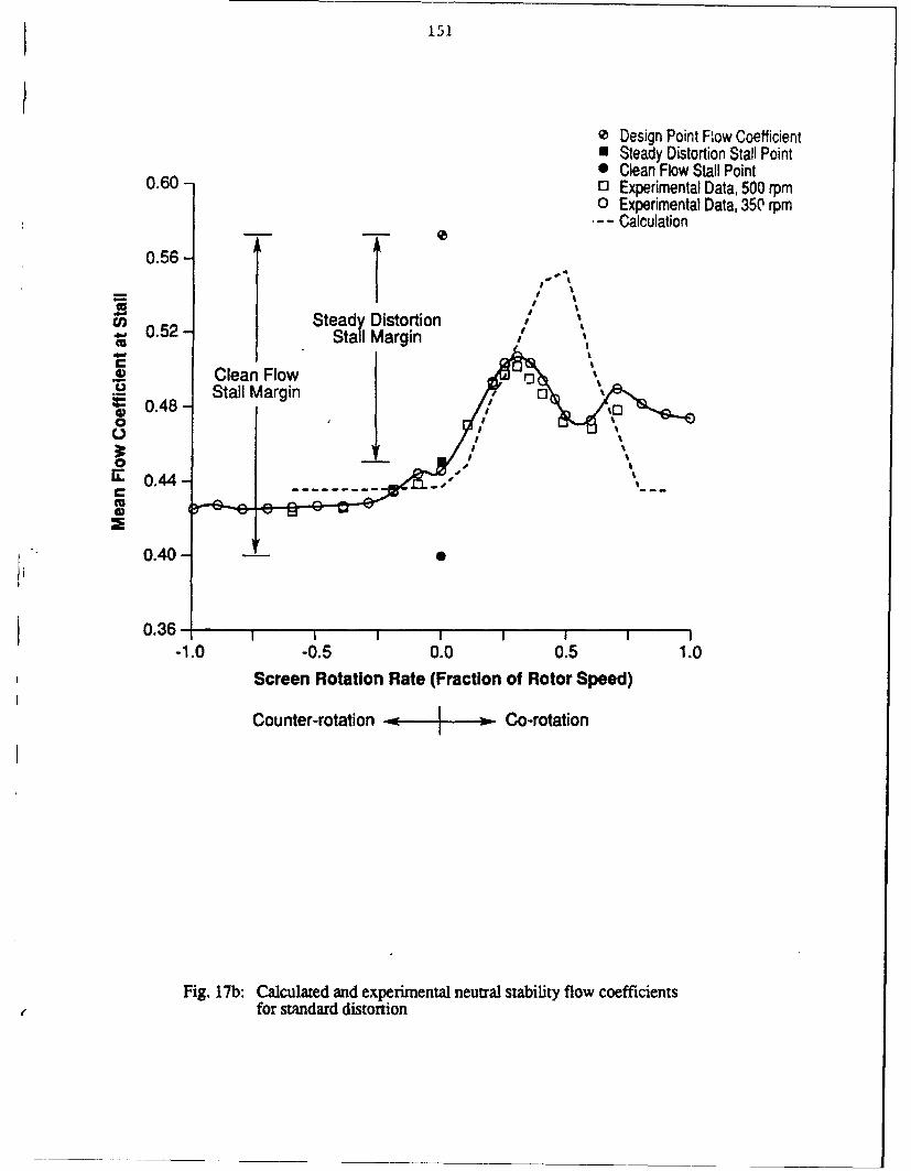
I 151
* Design Point Flow Coefficient* Steady Distortion Stall Point* Clean Flow Stall Point
0.60 13 Experimental Data, 500 rpmo Experimental Data, 350 rpm- - Calculation
0.56-
0.52- Stall Margin
i I
SCleaný Flow0
"Stall Margin 0S0.48 -0
IL 0.44 - .'=a
0.40-
0.36-"
-1.0 -0.5 0.0 0.5 1.0
Screen Rotation Rate (Fraction of Rotor Speed)
Counter-rotation . Co-rotation
Fig. 17b: Calculated and experimental neutral stability flow coefficientsfor standard distortion

152
- .. I I I , I.l L I i. .I , I , I , Il ,
C: o
t r).00
C -
(I)00
cri._)
CU -
E
Lo50 0
SZ
I-
* Cn 0• O O
JIleS I lu W8o3149o0 MOI.-

153
Imo -A-
00
o 04- L..
3 0
4r- ui
0 06
00o~0.
E u-Ln *0
00x z
00
C3C
oo C-
- 0 C
00el le l4'180 0
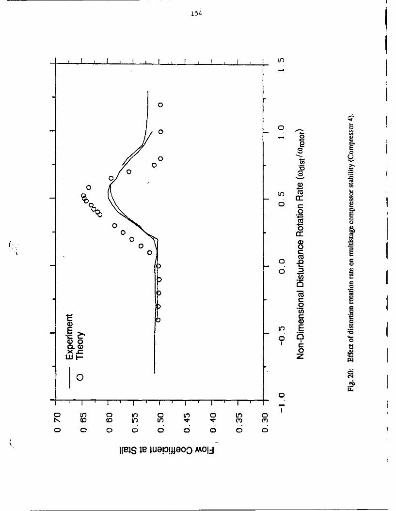
154
t I i I i I i i I0
00
0 -
o0L0~
0 LOo
0 z- j
0 0
co00
LO
(D 0
h.. 0
-. 0
a)ý
0~I LO D n o 00 0 (D V)4l C) Y
0) 0 0C
0.0ls leUaoWOOM
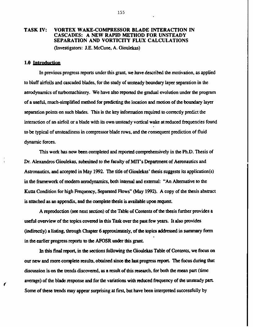
155
TASK IV: VORTEX WAKE-COMPRESSOR BLADE INTERACTION INCASCADES: A NEW RAPID METHOD FOR UNSTEADYSEPARATION AND VORTICITY FLUX CALCULATIONS(Investigators: J.E. McCune, A. Gioulekas)
1.0 Zn1dn, .i
In previous progress reports under this grant, we have described the motivation, as applied
to bluff airfoils and cascaded blades, for the study of unsteady boundary layer separation in the
aerodynamics of turbomachinery. We have also reported the gradual evolution under the program
of a useful, much-simplified method for predicting the location and motion of the boundary layer
separation points on such blades. This is the key information required to correctly predict the
interaction of an airfoil or a blade with its own unsteady vortical wake at reduced frequencies found
to be typical of unsteadiness in compressor blade rows, and the consequent prediction of fluid
dynamic forces.
This work has now been completed and reported comprehensively in the Ph.D. Thesis of
Dr. Alexandros Gioulekas, submitted to the faculty of MIT's Department of Aeronautics and
Astronautics, and accepted in May 1992. The title of Gioulekas' thesis suggests its application(s)
in the framework of modem aerodynamics, both internal and external: "An Alternative to the
Kutta Condition for high Frequency, Separated Rows" (May 1992). A copy of the thesis abstract
is attached as an appendix, and the complete thesis is available upon request.
A reproduction (see next section) of the Table of Contents of the thesis further provides a
useful overview of the topics covered in this Task over the past few years. It also provides
(indiectly) a listing, through Chapter 6 approximately, of the topics addressed in sunmmary form
in the earlier progress reports to the AFOSR under this grant.
In this final report, in the sections following the Gioulekas Table of Contents. we focus on
our new and more complete results, obtained since the last progress report. The focus during that
discussion is on the trends discovered, as a result of this research, for both the mean part (time
average) of the blade response and for the variations with reduced frequency of the unsteady part.
Some of these trends may appear surprising at first, but have been interpreted successfully by

156
Gioulekas in his thesis. In addition, some very interesting "rules of thumb" have emerged for the
steady (time average) circulation, or turning, that a loaded blade can create in an unsteady flow
environment.
2.0 Overview of Completed Research
A brief summary of the research accomplished under this Task is effectively provided by
the Table of Contents of Gioulekas' thesis:
Table of Contents
1 Introduction 141.1 Survey of previous work and connection to the present work 141.2 Synopsis of the thesis 291.3 Overview 32
2 Flow in a boundary layer with a rapidly oscillating free-stream velocity 332.1 Assumptions 332.2 The division of the flow-field 342.3 The non-dimensional form of the equations 412.4 The solution 482.5 Zero-th order approximation 492.6 Second order approximation 51
3 Unsteady separation 593.1 Conditions for unsteady separation 59
4 A criterion for predicting unsteady separation 714.1 Derivation of the criterion 714.2 Nondimensional form of te unsteady separation criterion 79
5 How the interaction between the airfoil and its wake determines the airfoilcirculation and the force and moment acting on the airfoil 835.1 The circulation 845.2 Airfoil in oscillating stream vs. oscillating airfoil in steady stream. what
is the difference in the aerodynamic force and moment? 915.3 Inertial and airfoil frames of reference 925.4 Calculation of the force using the unsteady Bernoulli equation 93
5.4.1 The pressure coefficient 935.4.2 The mapping of the physical to the circle plane 955.4.3 The force and moment coefficient 96
5.5 Calculation of the force using the impulse 965.6 Calculation of the moment using the moment of impulse 1005.7 The free wake convection 104
* Extracted from Gioulekas' Ph.D. Thesis. The page numbers refer to the thesis, not to this report.

157
6 The influence of reduced frequency, strength of flow unsteadiness, andellipse slenderness on unsteady separation 1066.1 Comparison between theoretical predictions and experiment 1066.2 The influence of the strength of the unsteadiness on unsteady separation 1236.3 The influence of the reduced frequency on unsteady separation 1296.4 The influence of ellipse slenderness on unsteady separation 132
7 A parametric study of the circulation and of the aerodynamic forcesacting on an airfoil in unsteady separated flow 1437.1 How the separation trajectories influence circulation 1357.2 The time evolution of the aerodynamic forces with varying angle of attack 1397.3 The influence of the reduced frequency on the aerodynamic forces 1457.4 The influence of the strength of the flow unsteadiness on the
aerodynamic forces 152
8 Conclusions and recommendations for future research 1588.1 Conclusions 1588.2 Suggestions for future research 160
A Why the boundary layer cannot be divided when the reduced frequency is low 168
B A simplification in the "Stokes equations" 171
C The nondimensional form of the "Prandtl velocity" distribution 173
- End -
The results discussed in the following sections are selected primarily from Chapters 6 and
7 of the above thesis.
3.0 T raectnries of the Up &.nn r uf e S ra on P it
on Bluff Airfoils or Blades at Angle of Attack
Application of the generally accepted separation criteria for unsteady boundary layer flow
for practical problems involving blade-wake interaction has long been recognized as quite
complex. Direct numerical study has been awkward, time consuming and expensive, with results
that are both difficult to interpret and to generalize.
But in the research reported in Gioulekas' thesis, and in our earlier progress reports to
AFOSR, we have been able to achieve a substantial simplification of this computational task
without sacrificing the important physics involved. This is particularly so when the unsteadiness
occurs at moderately high "reduced frequencies", woc/U > 1, for reasons originally pointed out

158
separately by C.C. Lin and by Lighthill. In addition to the simplifications suggested by Lin, we
have been able to add an extension of the ideas of Stratford* to provide an algebraically simple
computational criterion for separation, involving only external par4meters of the flow, steady or
unsteady.
The result is that we can now readily calculate the instantaneous location and motion of the
boundary layer separation point(s), without having to go through a complete boundary layer
calculation at each time step. This means that when a blade or an airfoil is interacting with its own
unsteady wake, the effect of the wake itself, back on the boundary layer that is "feeding" it, can be
readily included, and this is a key feature of the results reported here.
The examples included below illustrate the kind of separation trajectories one finds above a
slender, bluff airfoil in unsteady flow, and how these depend on some of the key parameters
involved. The first cases shown are for an ellipse of slenderness ratio 1:20 at zero mean angle-of-
attack. In that case, of course, the separation trajectories on the lower surface of the blade are the
mirror image of those shown here. Results for finit mean angle-of-attack are discussed in the
following section, in terms of the blades' aerodynamic response, both for the steady and for the
unsteady component.
The value of the reduced frequency, wc/U.0 , in the first case shown for this section, is
-U.
and results are shown as a function of the strength of the unsteady oscillations, as measured by
Here, c is the airfoil chord and the external flow is U.0 = U.. + 0. ei(O)t +.
Figure 1, extracted from Chapter 6 of the thesis, shows separation point trajectories near
the ellipse's trailing edge for e = 0.01, 0.005, 0.001, and 0. The a separation point, as
* An extensive bibliography is provided in Gioulekas' thesis, and has also been made available in
earlier AFOSR progress reports. A feature of Gioulekas' thesis, in fact, is the usefulness of hisbibliography.

159
calculated by Howarth (see discussion in previous reports, or in the thesis), is also shown for
reference. Each trajectory shown represents the path traversed by the separation point over one
period of oscillation.
The figure shows that as the strength or amplitude of unsteadiness decreases from 1% to 0,
the trajectories shrink in range and converge on the steady-flow separation point, as would be
expected. However, one also readily sees that not all effects are simpiy "linear" in e.
Figure 2 gives corresponding results for fixed e, but with varying reduced frequencies,
ranging from 9 to 36. At first, these results may seem surprising, because one sees that as the
frequency increases at fixed amplitude, the trajectories again converge toward the steady-flow
separation location.
This phenomenon is explained by Gioulekas in his thesis. In simple terms, at high
frequency the response of the unsteady part of the flow to the wall's resistance is confined to an
ever-thinner sheath, analogous to Stokes flow for an oscillating infinite wall. In the limit, this inner
sheath becomes decoupled from the "Prandtl-type" boundary layer, which is the part of the flow
that responds primarily to the steady part of the wall's resistance, that is, to the mean (time-
averaged) flow. Thus, at very high reduced frequencies, the "Stokes layer" and the "Prandtl layer"
become decoupled, and in the limit, the boundary layer separation properties are determined
completely by the mean flow, precisely becaus the frequency is high.
4.0 Aerodynamic Resnos for Leaded S en Bla
With the new method made available by his analysis of the problem, and by his
corresponding extension of the "Stratford Criterion" to unsteady flow, Gioulekas was able to
systematically investigate the aerodynamic response of bluff-edged airfoils over a range of blade
slenderness and of mean angle-of-attack.
As we have pointed out in our earlier reports, the new method of rapid location of the
separation trajectories plays the same role in determining the blade cir. ulation as does the classical
Kutta condition for unseparated, sharp-edged blades or airfoils. It is natural, therefore, to compare

160
the results Gioulekas obtained with those that would be obtained if the Kutta condition were
assumed to apply.
A second benchmark is the circulation that would be obtained in steady flow over the
separated bluff airfoil at angle-of-attack, as first obtained by Howarth.
With these limits in mind, Tables 1 and 2 provide useful and revealing summary
information to guide our understanding of blade performance in unsteady flow.
In Table 1, the results for an elliptic airfoil of fineness 1:20, at angle-of-attack = 50, and for
an amplitude of unsteadiness E = 0.04, are shown for a range of reduced frequencies. Tabulated
are the mean (time-averaged) circulation F developed by the blade, the time-varying circulation r,
and the phase-shift, to be compared with classical unsteady airfoil theory. The values on the left
are those that are obtained if the Kutta condition is (arbitrarily) assumed. Those on the right are the
responses obtained using the present theory, and are thus based on-the more realistic prediction of
the instantaneous location and movement of the boundary layer separation point(s).
We note that the values of F actually achieved by the blade are systematically lwr than
those it "could" achieve if Kutta applied.
We also note that rlow-mh, the steady flow value of circulation obtained by the same
airfoil, at the same angle-of-attack, taking into account the separation of the upper-surface
boundary layer, would be
rHowarth = 0.267
about 8% less than rKuta. Based on our observations of the separation trajectories described in
Section 3.0, it is clear why, as the frequency increases, the actual F approaches the lower,
separated steady-flow value, rIowal, for a bluff-edged airfoil.
In any case, the results provide us with useful bounds for the mean circulation obtainable
by a bluff-edged blade at angle-of-attack in any unsteady environment:
rHowarth • F • rKu •
These bounds can be used, for example, to estimate the maximum loss of mean turning angle that
might occur in a blade row as a result of unsteadiness. The higher the frequency, the closer the

161
jloe value is approached. And, at fixed frequency, the thinner the blade, the more closely rKuta
can be obtained.
Table 2 serves as one check on the theory, and verifies that, as the blade is chosen thinner
and thinner, conditions approach those appropriate to the classical Kutta condition, other
parameters being held constant. This is true not only for the mean circulation, F, but also for the
properties of the unsteady component of the blade response. The amplitudes 1f, and the phase
angles Or, obtained from the new theory, agree remarkably well , for very thin elliptical blades,
with the results of classical thin airfoil theory. Table 2 shows this agreement for the example of an
elliptical blade of fineness ratio 1:50, at reduced frequency X2 = 9.
Summary conclusions of the kind given in the above two tables were obtained by
systematic study of the results obtained for many cases (each for a given set of the above-
mentioned parameters) by runs such as are illustrated in Figs. 3 through 5. These figures show
how the aerodynamic responses were actually obtained and analyzed, and illustrate only a small
sample of the results reported by Gioulekas.
5.0 Future and Ongoing Anplications
The extensive results available in Gioulekas' thesis represent a substantial study of the
blade-wake interaction effect for driven, or imposed, unsteady oscillations, including realistic
treatment of the boundary layer separation properties.
Future work includes application of this technique to the determination of natural-
oscillation regimes (analogous to the Karman vortex street behind a cylinder) for thin elliptical
blades or airfoils.
The method also has direct application to the dynamic stall problem for airfoils in external
flow.

162
(a) Kutta Condition (b) Separation
X2 r I r 0 r Or9 0.288 0.0015 _500 0.279 0.003 -460
18 0.288 0.001 -520 0.272 0.002 -590
36 0.288 0.0005 -54o 0.271 0.001 -650
TABLE 1: The circulation 1"(t) - 1 + r7 cos(ot + Or) around an ellipse calculated by: (a)assuming smooth flow at the trailing edge, and (b) using the new separation criterion,as the reduced frequency increases (b : a = 1 : 20, a = 50, E = 0.04). Note that
- Howarth = 0.267 as the reduced frequency increases.
Slenderness (a) Kutta Condition (b) Separation
Ratio r 9hr Or
1:20 0.288 0.0015 -50o 0.279 0.003 -460
1:50 0.279 0.002 -46° 0.279 0.002 -46o
TABLE 2: The circulation 1F(t) = r + f cos(ot + Or) around an ellipse calculated by: (a)assuming smooth flow at the trailing edge, and (b) using the new separation criterion,as the ellipse becomes slimmer (a = 5P, X2 = 9, e = 0.04).
* All "1 values" presented here are made dimensionless with U.,c, i.e., each number is(circulation)/U.c.
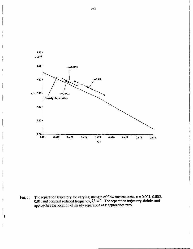
163
x10-36.60. = .0$.lO3 t-.O
3.20,- 4=0-01
y/C 7.90- 4=0.001
Steady Separtion
7.30
7.000.471 0.472 0.473 0.474 0,475 0.476 0.4" 0.471 0.479
X/€
Fig. 1: The separation trajectory for varying strength of flow unsteadiness, e = 0.001, 0.005,0.01, and constant reduced frequency, X2 = 9. The separation trajectory shrinks andapproaches the location of steady separation as e approaches zero.

164
x 10-3
2.40,i
2.00.
1.60-
7/C 1.20 - A3=18
4 ~0.40.I
0.00.10.460 0.465 0.470 0.475 0.480 0.485 0.490 0.495 0."00
x/c I
I
I
Fig. 2: The separation trajectory for varying reduced frequency, X2 = 9, 18, 36, and constantstrength of flow unsteadiness, e = 0.04. The amplitude of the separation point excursionscales with I42. 1

165
x 10-21.(000.80
Steady 3#1P&I&I •on %=3•.T/4 M=0
Y/4 0.60
0.40
0.20
0.000.46 0.465 0.470 0.475 0.480 0.485 0.490 0.495 0.500
I/C
0.288
0.286
0.284
0.232
0.2?8
0.278
0.0 0.5 1.0 1.5 2.0 2 5 3 0 3.5 4.0s/T
I
Fig. 3: The stationary points t = T/4,/; t = 3T/4 of the suction-side separation trajectory roughlycorrespond to the stationary points in r*(t). The ellipse (b/a = 1 : 20) is placed at anangle of attack a = 50 in a stream oscillating with strength e = 0.04 at reduced frequencyX2 = 9.

166
0.296.
01959
0,290, -ee A2= :18
0.290 (. 1& A2 = 3
0.235.
r 0.280
0.270
0.0 0.5 1.0 1.5 2.0 2.5 3.0 3.5 4.0t/T
Fig. 4: Time evolution of the non-dimensional circulation for varying reduced frequency (X2 =9,18, 36) and constant strength of flow unsteadiness (e = 0.04). The circulation isbracketed by rKuta = 0.283 and FHowarth = 0.267. The ellipse (b/a = 1 : 20) is at anangle of attack x = 5Y.
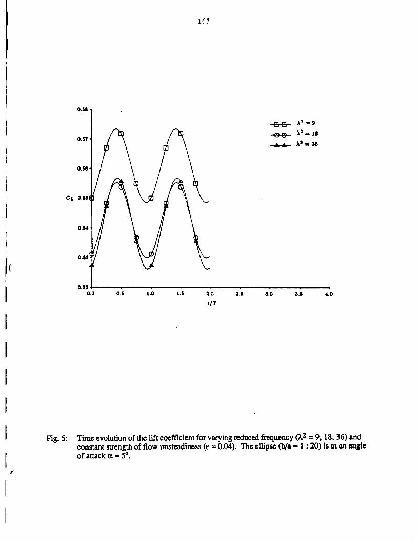
167
O.58
O.-e A2 = IS
0.57 2 183
0.56-
C1, 0.55EAl
0.54-
0.53
0.52.0.0 0.5 1.0 1.5 3.0 2.5 8.0 3.5 4.0
t/T
Fig. 5: Time evolution of the lift coefficient for varying reduced frequency (X2 :9, 18, 36) andconstant strength of flow unsteadiness (e = 0.04). The ellipse (b/a = 1 : 20) is at an angleof attack a = 50.
168
APPENDIX IV.l
An alternative to the Kutta conditionfor high frequency, separated flows
by
Alexandros Gioulekas
Submitted to the Department ofAeronautics and Astronautics
in partial fulfillment of therequirements for the Degree of
Doctor of Philosophy
Abstract
An alternative to the Kutta condition for determining the circulation around a bluffairfoil in unsteady, separated flow is presented. For such flows, there is a need for apractical criterion which would avoid the detailed boundary layer calculations and wouldpredict the time evolution of the airfoil circulation based on the external potential flowonly.
This criterion would play for unsteady, separated flows the role that the Kuttacondition plays for flows past thin airfoils. It turns out to be a criterion for predictingthe location and movement of the "separation points', because they determine the netvorticity flux shed into the wake and thus the rate of change of the airfoil circulation.
The laminar, two-dimensional flow about a bluff airfoil at angle of attack, when theexternal flow oscillates at a high reduced frequency is considered.
At high frequencies, the vorticity generated as the wall resists the imposed unsteadi-ness is confined to a thin layer near the blade surface ("Stokes layer") and its contri-bution to the displacement thickness is proportional to an inverse power of the reducedfrequency and thus small. Outside this region, the unsteady part of the boundary layervelocity is approximately the external potential oscillation. Based on this observationand following C.C. Lin, the boundary layer velocity can be divided into two coupledvelocity distributions, one predominantly oscillatory (IStokes velocity') and anotherpredominantly steady ('Prandtl velocity'). The main contributor to the displacement /thickness is the latter. Therefore, separation, identified by a dramatic increase in the 'displacement thicknem, can be located by calculating the evolution of the 'Prandtlvelocity'and finding where the latter bifurcates.
/( Stratford's ideas, modified to account for unsteadiness in the "Prandtl velocity'
I

169
(arising through the coupling of the "Prandtl" to the "Stokes" flow by the no-slipcondition on the wall and Reynolds-stress terms in the momentum equation), lead toa criterion for unsteady separation that uses as only inputs parameters of the externalflow and avoids a detailed boundary layer calculation.
The airfoil circulation is calculated by an iterative method which calculates how theinteraction between the airfoil and its wake affects separation.
An ellipse is adopted as a study case, and results are presented for varying angleof attack, ellipse slenderness, reduced frequency, and strength of unsteadiness. In thelimit of a very slender ellipse, the theory recovers the results from the classical unsteadywing theory, which assumes the Kutta condition.
The theory predicts that there exist two limits for the mean value of the circulation.The upper limit is the value of the circulation for which the trailing edge becomes astagnation point (rKutt.). The lower limit is the value of the circulation in steady flow
The pressure-side "separation point" for all practical purposes can be consideredfixed, even at small angles of attack. On the other hand, the "separation point" on thesuction-side oscillates with amplitude proportional to the strength of the flow unsteadi-ness, and inversely proportional to the reduced frequency. When the reduced frequencyincreases or the strength of flow unsteadiness decreases, the trajectory of this "separa-tion point" shrinks and tends toward the position of steady separation. Since the meanlocation of the suctiou-side "separation point" controls the mean value of the circu-lation, and the amplitude of its excursion determines the amplitude of the oscillatorycomponent of the circulation, the above trends explain how the circulation responds tochanges in the flow unsteadiness.
Thesis Supervisor: James E. McCune
Title: Professor of Aeronautics and Astronautics

179
3. AIR FORCE RESEARCH IN AERO PROPULSION TECHNOLOGY
(AFRAPT) PROGRAM
The research at MIT is strongly tied in with the AFRAPT Program. The students who
have participated in this program during the contract period, the advisors, and the research projects
are:
Trainee: Jabin BellAdvisor: Prof. A.H. EpsteinProject: Active Control of Jet Engine Surge
Trainee: Aaron Gleixner (finished M.S. Thesis, 8/92)Advisor: Prof. A.H. EpsteinProject: Unsteady Phenomena in Transonic Axial Flow Turbines (RR)
Trainee: Martin GrafAdvisor: Prof. A.H. EpsteinProject: Characterization of Fully Scaled Turbine Blade Boundary Layers
Trainee: Daniel Gysling (finished M.S. Thesis, 8/89; Ph.D. expected, 8/93)Advisor: Prof. J. Dugundji/Prof. E.M. Greitzer/Prof. A.H. Epstein/Prof. J. KerrebrockProject: Active and Structural Control of Aeromechanical Systems (AFOSR)
Trainee: Dana Lindquist (finished Ph.D. Thesis, 12/91)Advisor: Prof. M.B. GilesProject: Development of Adaptive Procedures for Turbomachinery Flow Computations
Trainee: Knox Millsaps (finished Ph.D. Thesis, 5/92)Advisor: Prof. M. Martinez-SanchezProject: Rotor Dynamic Instability Due to Alford Forces (NASA MSFC)
Trainee: G. Scott McNultyAdvisor: Prof. E.M. GreitzerProject: Self-Adaptive Aeropropulsion Components
Trainee: Taras Palczynski (finished M.S. Thesis, 8/92)Advisor: Prof. M. Martinez-SanchezProject: Tip Clearance Excited Turbomachine Rotordynamic Instabilities (NASA MSFC)
Trainee: George Pappas (finished M.S. Thesis, 8/90)Advisor: Prof. A.H. EpsteinProject: Temperature Distortion Effects on Turbine Heat Transfer (RRI)

17J
Trainee: Peter Silkowski (finished M.S. Thesis, 2/90; left MIT, 8/92)Advisor: Prof. E.M. Greitzer/Dr. C.S. Tan/Prof. N.A. Cumpsty (Cambridge University)Project: Unsteady Phenomena and Flow Instabilities in Multistage Turbomachines
(AFOSR)
A more detailed description of the work carried out on these projects is given in Refs. 3.1
3.2, and 3.3.
References
3.1 Greitzer, E.M., Dugundji, J., Epstein, A.H., Giles, M.B., Martinez-Sanchez, M., Tan, C.S.,"Air Force Research in Aero Propulsion Technology," Annual Technical Report on GrantAFOSR-85-0288, September 1990.
3.2 Greitzer, E.M., Dugundji, J., Epstein, A.H., Giles, M.B., Martinez-Sanchez, M., Tan, C.S.,"Air Force Research in Aero Propulsion Technology," Annual Technical Report on GrantAFOSR-91-0052, September 1991.
3.3 Greitzer, E.M., Dugundji, J., Epstein, A.H., Giles, M.B., Martinez-Sanchez, M., Tan, C.S.,"Air Force Research in Aero Propulsion Technology," Annual Technical Report on GrantAFOSR-91-0052, October 1992.

172
4. PUBLICATIONS AND PRESENTATIONS (Period 10/91 - 10/92)
Epstein, A.H., "Unsteady Effects in Turbine Aerodynamics and Heat Transfer," ASEA BrownBoveri Research Laboratory, Baden, Switzerland, October 1992.
Fritsch, G., Giles, M., "Second-Order Effects of Unsteadiness on the Performance ofTurbomachines," ASME Paper 92-GT-389, presented at the International Gas Turbine andAeroengine Congress and Exposition, Cologne, Germany, 1992.
Giles, M.B., "An Approach for Multi-Stage Calculations Incorporating Unsteadiness," ASMEPaper 92-GT-282, presented at the International Gas Turbine and Aeroengine Congress andExposition, Cologne, Germany, 1992.
Giles, M.B., "Current Status of CFD Capability for Unsteady Flow Analysis," presented atNASA Lewis Workshop on "Unsteady Flow in Turbomachines: Potential Benefits, PresentStatus, Future Research", May 1992.
Greitzer, E.M., Tan, C.S., "Unsteady Flow in Turbomachines: Where's the Beef?", presented atNASA Lewis Workshop on "Unsteady Flow in Turbomachines: Potential Benefits, PresentStatus, Future Research", May 1992.
Guenette, G.R., Pappas, G., Epstein, A.H., "The Influence of Non-Uniform Spanwise InletTemperature on Turbine Rotor Heat Transfer," presented at 80th PEP/AGARD Symposium,Antalya, Turkey, October 1992.
Longley, J.P., Greitzer, E.M., "Inlet Distortion Effects in Aircraft Propulsion System Integration,"AGARD Lecture Series 183 on "Steady and Transient Performance Prediction of Gas TurbineEngines," June 1992.
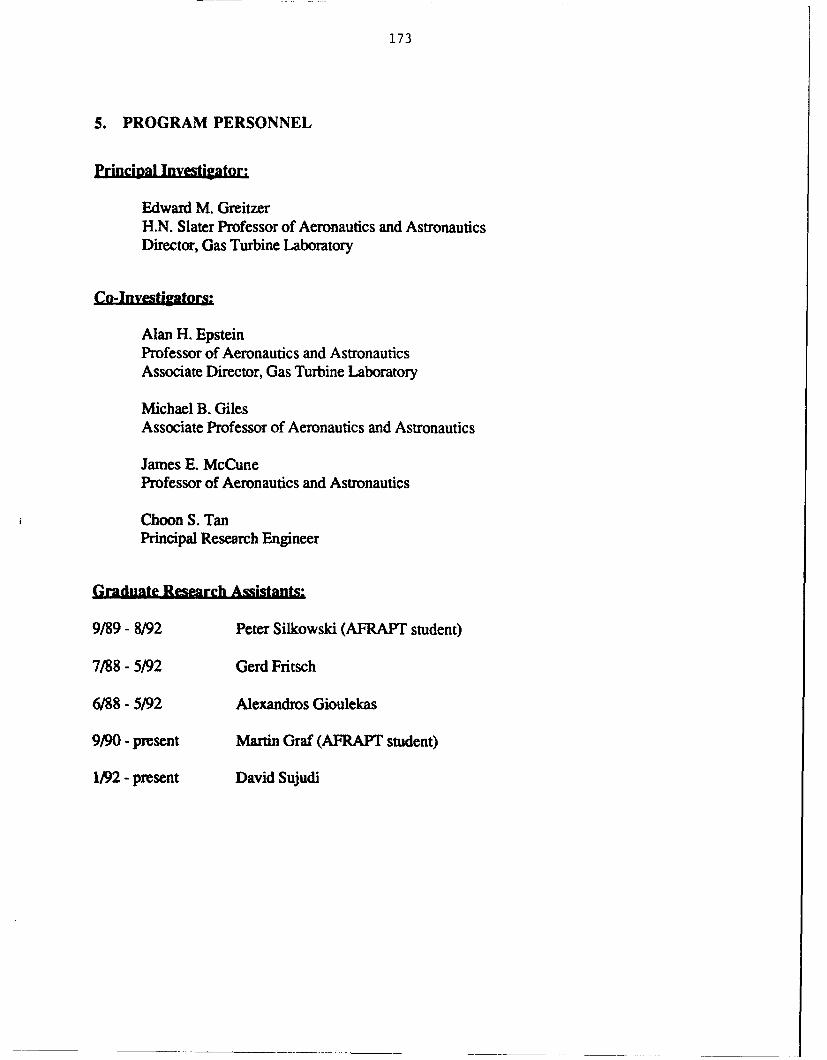
173
5. PROGRAM PERSONNEL
Principal Investigator:
Edward M. GreitzerH.N. Slater Professor of Aeronautics and AstronauticsDirector, Gas Turbine Laboratory
Co.-Investigators:
Alan H. EpsteinProfessor of Aeronautics and AstronauticsAssociate Director, Gas Turbine Laboratory
Michael B. GilesAssociate Professor of Aeronautics and Astronautics
James E. McCuneProfessor of Aeronautics and Astronautics
Choon S. TanPrincipal Research Engineer
Graduate Research Assistants:
9/89 - 8/92 Peter Silkowski (AFRAPT student)
7/88-5/92 Gerd Fritsch
6/88 - 5/92 Alexandros Gioulekas
9/90 - present Martin Graf (AFRAPT student)
1/92 - present David Sujudi

174
6. INTERACTIONS
As we have noted previously and as may be inferred from the presentations that were
given, there are considerable interactions between Gas Turbine Laboratory personnel and industry
and government, as well as with other universities. This occurs in several forms. One of these is
collaborative research projects with industry and government laboratories. This creates a direct
link with those persons who are actively working in similar areas in other establishments, and aids
considerably in helping transfer technology.
A second type of interaction is through presentations and discussions with industry or
government agencies. These were listed in Section 4 covering the contract period. It should be
noted that Qnly those which involved discussion of the work supported by AFOSR under this
grant are given.
The Gas Turbine Laboratory also has an active seminar program which brings speakers
from industry and government. The speakers for the past ,ear are listed below; those for previous
years have been listed in Refs. (6.11 and [6.21.
Mr. W. Culhane, American Airlines"Today's Centralized Fault Detection System, Maximum InformationYielding Minimum Value"
Mr. B. Koff, Pratt & Whitney Aircraft"Spanning the Globe with Jet Propulsion"
Mr. J. Kuhlberg, Pratt & Whitney Aircraft"Jet Engine Controls: Past, Present, and Future"
Dr. D. McCormick, United Technologies Research Center"Vortical and Turbulent Structure of Lobed Mixer Free Shear Layers"
Dr. L. Nichols, NASA Lewis Research Center"Numerical Propulsion System Simulation" IAs mentioned in the description of Task III, there is strong coupling with the Whittle
Laboratory at Cambridge University. This laboratory is of comparable size to the Gas Turbine
Laboratory and has an excellent and very active group of faculty and students focussed on

175
turbomachinery research. Another close interaction which spans several of the tasks is with
Professor F.E. Marble of Caltech. Marble is the former Head of the Jet Propulsion Center in the
Division of Engineering and Applied Sciences, and has worked on a wide range of fluids
problems connected to propulsion. He has participated in discussions in the Gas Turbine
Laboratory for over a decade, and his physical insight and ability to penetrate to the heart of
complex issues have been enormously helpful to us in that time.
E. M. Greitzer spent a month at the Ohio Aerospace Institute as a Lecturer in Residence on
Turbomachinery. This included a series of lectures on turbomachinery aerodynamics at NASA
Lewis Research Center, as well as lectures and discussions with industry and government
laboratories and universities in the Ohio region: General Electric Aircraft Engines, Wright
Laboratories, Allison Gas Turbine Division, University of Cincinnati, and Case Western Reserve
University.
E.M. Greitzer, C.S. Tan, and M.B. Giles participated in a NASA/industry/university
workshop on unsteady flow in turbomachines. The purpose of the workshop was to assess
available information on the importance of unsteady flow in practical turbornachines and see
whether a consensus existed on the magnitude of the gains to be achieved through better
understanding of unsteady flow, and the issues that were central to the potential gains. A further
goal was to define and prioritize those fluid dynamic topics in unsteady flow on which attention
should be focused. The participants had strong consensus that critical unsteady flow problems,
with substantial payoff, exist in the areas of gas turbine engine and compressor stability, and in
aeroelasticity in turbomachines. Much of the discussion, therefore, was aimed at the area of
greatest uncertainty, the unsteadiness associated with rotor stator interaction, i.e. unsteady flow
effects which have a length scale on the order of the blade pitch.
A report on the workshop has been written by J.J. Adamczyk (NASA), A.J. Strazisar
(NASA) and E.M. Greitzer (MIT). A summary of this report is given below:

176
SummaryNASA Government/Industry/University Workshop on
Unsteady Flow in Turbomachines: Potential Benefits, Present Status, Future Research
On May 20-21, 1992 a workshop was held at NASA Lewis Research Center on the topicof "Unsteady Flow in Turbomachines". The purpose of the meeting was to bring together activeworkers in the field, from university, industry, and government, to address the followingquestions:
1. What areas show potential for gas turbine engine performance increase through improved
understanding of unsteady flow?
2. What are the magnitude of the gains to be expected?
Associated with the answers to (1) and (2) are several follow-on issues:
3. What is the current state of the art in understanding in the areas defined to be of importance?
4. What topics should be explored further?
5. How does one do this in an appropriate manner (What is the balance of basic and appliedresearch, near term versus long term, etc.)?
6. If C.F.D. codes are to be used to quantify the effects of unsteady flows on aero-performanceand surface heat transfer, how should these codes be calibrated?
A. H. Epstein participated in a study of wide breadth carried out by the Aeronautics and
Space Engineering Board of the National Research Council. The purpose was to assess the current
state of aeronautics in the United States and to help identify the technology advances necessary to
meet the challenges of the next several decades. The conclusion of the study are summarized in
the report "Aeronautical Technologies for the Twenty-First Century" issued by the ASEB.
E. M. Greitzer participated in an Air Force Scientific Advisory Board Committee to
examine failures in titanium components of Air Force aircraft engines.

Reference
6.1 Greitzer, E.M., Epstein, A.H., Giles, M.B., McCune, J.E., Tan, C.S., "Unsteady FlowPhenomena in Turbomachines," Annual Technical Report on Grant AFOSR-90-0035,November 1990.
6.2 Greitzer, E.M., Epstein, A.H., Giles, M.B., McCune, J.E., Tan, C.S., "Unsteady FlowPhenomena in Turbomachines," Annual Technical Report on Grant AFOSR-90-0035,December 1991.

178
7. DISCOVERIES, INVENTIONS, AND SCIENTIFIC APPLICATIONS
During the present contract period, there have been no inventions.

179
8. CONCLUDING REMARKS
Several aspects of the multi-investigator program deserve comment. First, one can see
explicitly in the research conducted strong technical links with industry and government
laboratories. A consequent benefit is the connection with problem areas that are of real interest;
this is useful and stimulating to faculty and students alike. A second positive feature is that there
are personnel at these organizations who are directly involved in the programs. These people are,
within the organizations, the "owners" of the scientific and engineering results that emerge from
the research. In this sense, there is much less need for other formal mechanisms for technology
transition, since this occurs at the grass roots level.
Another item is the strong coupling between investigators, which has been fostered by this
program. We believe this is extremely useful in "cutting edge" aeropropulsion research; the
problems are not only conceptually difficult, but are also complex. Having several different types
of talents focussed on the different areas provides a substantial synergism to the overall program.
The multi-investigator aspect of the research program is a powerful resource,