Accruals, Free Cash Flows, and EBITDA for Agribusiness

Firms

Carlos Omar Trejo-Pech1

Richard Weldon2

Lisa House2

Tomás Salas-Gutiérrez3

Selected Paper prepared for presentation at the American Agricultural Economics Association Annual Meeting, Long Beach, California, July 23-26, 2006

1Food and Resource Economics Department, University of Florida, United States of America, and Escuela Empresariales, Universidad Panamericana at Guadalajara, México. 2Food and Resource Economics Department, University of Florida, United States of America 3Escuela Empresariales, Universidad Panamericana at Guadalajara, México Contact information: Food and Resource Economics Department at the University of Florida, Box 110240, Gainesville, FL 32611-0240, United States of America. ctrejo@ufl.edu Copyright 2006 by Trejo-Pech, Weldon, House, and Salas-Gutiérrez. All rights reserved. Readers may make verbatim copies of this document for non-commercial purposes by any means, provided that this copyright notice appears on all such copies.

Abstract

This study explores the relationships between the accrual and cash flow components of

earnings for agribusiness. Three accrual models with their respective cash flows, free

cash flows, and free cash flows to equity are analyzed. Results for the agribusiness

industry are compared with results from previous studies of all firms. Earnings Before

Interests, Taxes, Depreciation, and Amortization (EBITDA), a measure frequently

recommended as a proxy for cash flow is tested using these models. Empirical results

show that both the magnitude and the behavior of EBITDA differ from cash flows and

should not be used as a proxy.

Accruals, Free Cash Flows, and EBITDA for Agribusiness Firms

This study explores the relationships between the accruals and cash flows components of

earnings for agribusinesses using data covering the period 1962-2004. The definitions

and modeling of accruals versus cash flows by Healy (1985) and Sloan (1996) have been

considered the standard in the accounting economics literature. Recent introduction of a

more comprehensive model by Richardson (2005) proves to be useful in explaining

financial accounting and cash flow relationships by exploring accruals components other

than just current operating accruals (non-current operating accruals and financing

accruals). The most important contribution of the work by Sloan (1996) and Richardson

et al (2005) is the recognition that even though accruals provide valuable information

about current and future earnings, few decision makers pay attention to this information.

This study builds on these models by introducing a third measure of accruals as an

alternative to directly relate accruals to free cash flow. In addition, Earnings Before

Interests, Taxes, Depreciation, and Amortization (EBITDA), an accounting measure

frequently recommended as a proxy for cash flow is tested using these models.

The next section of the paper is devoted to discussing the methodology, including

variable measurement, models and a literature review. Then results are discussed for

different models and comparing results for agribusiness and for ‘all firms’ from previous

studies. Conclusions are provided.

- - 1

Data and Methodology

The data used in this study is from the CRSP/COMPUSTAT merged (CCM)

database1. The CCM database provides records of a firm’s financial statements and stock

prices from 1962 through 2004. Specifically, information from the balance sheet and the

income statements are used. Fama and French (1992) document that pre-1962 data have

serious selection bias towards large, historically successful firms. The sample includes

402 firms with 4,785 firms-year observations.

For the cross-sectional analysis all firms were ranked according to the size of

accrual component of their financial statements. The firms were then grouped into

portfolios with the smallest twenty percent in the first portfolio, the next twenty percent

in the second portfolio, and so on.

Variable Measurement

Standardized variables. All variables in the study are standardized by firm size to

allow for relative comparisons. Therefore, all financial measures are divided by average

total assets, or the average of beginning and ending total assets. This scaling of variables

has been documented as necessary to fix potential problems of heteroskedasticity of

undeflated earnings Beaver (1970), and to avoid spurious correlations due to size

Dechow (1994).

Accruals and Cash Flow. Accruals are the net effect of non-cash accounts

included in the calculations of earnings. Earnings and cash flows differ to the extent that

accruals change. In an infinite length financial period (or just one period accounting 1 SIC codes used in this study include 2000, 2011, 2013, 2015, 2020, 2024, 2030, 2033, 2040, 2050, 2052 2060, 2070, 2080, 2082, 2086, 2090, and 2092.

- - 2

system) earnings and accruals would be the same. This study uses three definitions of

accruals, each of them mapping a different business activity-related cash flow.

Definitions by Healy (1985) and Sloan (1996) contain the core components of what have

become synonymous with accruals in the accounting economics literature.

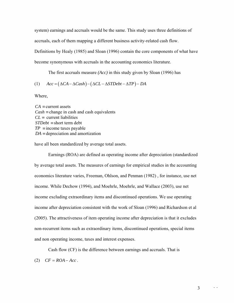
The first accruals measure (Acc) in this study given by Sloan (1996) has

(1) ( ) ( )Acc CA Cash CL STDebt TP DA= ∆ − ∆ − ∆ − ∆ − ∆ − Where, CA ≡ current assets Cash ≡ change in cash and cash equivalents CL ≡ current liabilities STDebt ≡ short term debt TP income taxes payable ≡DA ≡depreciation and amortization

have all been standardized by average total assets.

Earnings (ROA) are defined as operating income after depreciation (standardized

by average total assets. The measures of earnings for empirical studies in the accounting

economics literature varies, Freeman, Ohlson, and Penman (1982) , for instance, use net

income. While Dechow (1994), and Moehrle, Moehrle, and Wallace (2003), use net

income excluding extraordinary items and discontinued operations. We use operating

income after depreciation consistent with the work of Sloan (1996) and Richardson et al

(2005). The attractiveness of item operating income after depreciation is that it excludes

non-recurrent items such as extraordinary items, discontinued operations, special items

and non operating income, taxes and interest expenses.

Cash flow (CF) is the difference between earnings and accruals. That is

(2) CF . ROA Acc= −

- - 3

Accruals by definition represent outflows (negative accruals imply inflows). Thus

positive accruals decrease cash flows, and negative accruals increase them.

The second definition of accruals is a comprehensive accruals measure, recently

introduced in the literature by Richardson et al (2005). This total accruals model is an

extension of the work by Sloan (1996) and it allows for testing of accounting reliability.

Total accrual (TACC) is, (3) T ACC WC NCO FIN= ∆ + ∆ + ∆ with, (4) ( ) (

CO COA L

WC CA Cash CL STDebt= − − − )

(5) ( ) ( )

ANCO NCOL

NCO TA CA LTInv TL CL LTDebt= − − − − −

(6) ( ) (

FIN FINA L

)FIN STInv LTInv LTDebt STDebt PStock= + − + +

Where, TACC ≡ total accruals

WC∆ ≡ change in working capital NCO∆ ≡ change in net non-current operating assets FIN∆ ≡ change in net financial assets

COA ≡ current operating assets CA current assets ≡Cash cash and short term investments ≡COL ≡ current operating liabilities CL ≡ current liabilities STDebt ≡ short term debt NCOA ≡non-current operating assets TA ≡ total assets LTInv ≡ long term investment or investment and advances other NCOL ≡non-current operating liabilities TL ≡ total liabilities LTDebt ≡ long term debt

- - 4

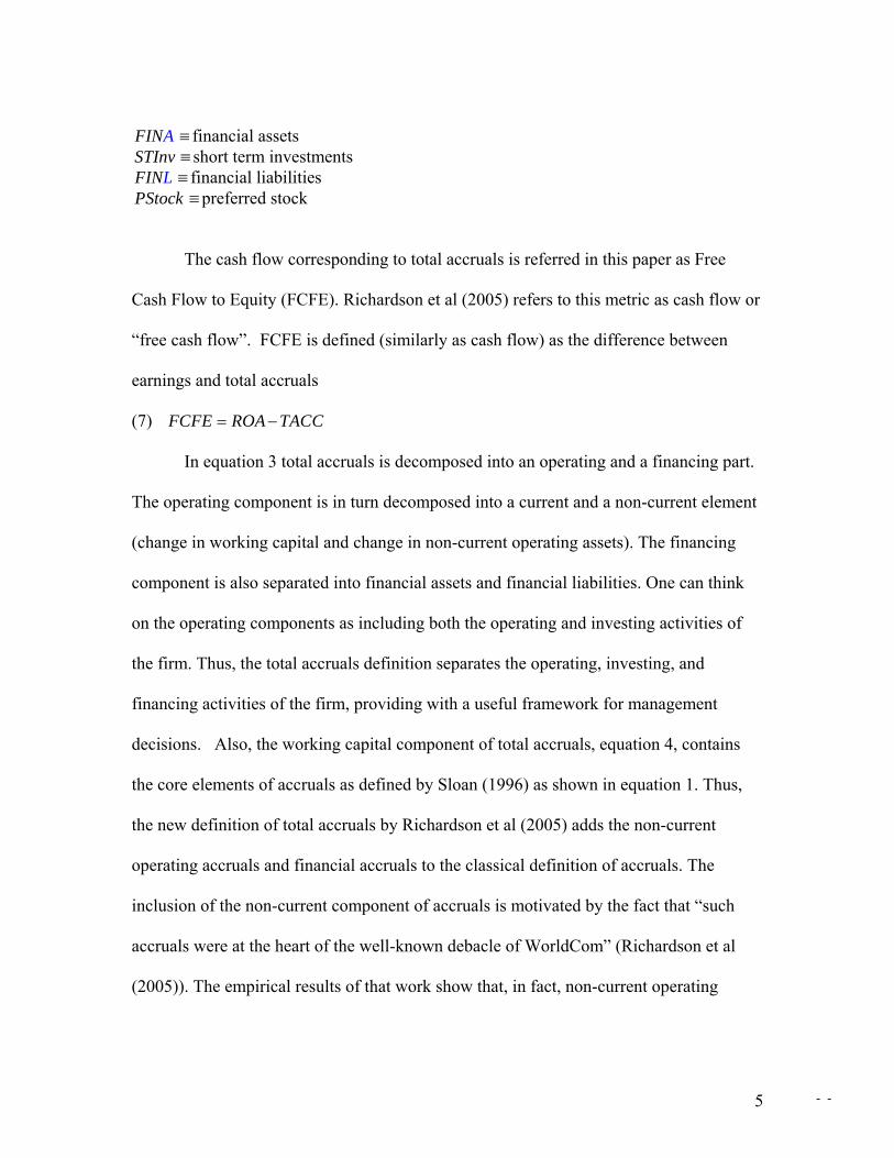
FINA ≡ financial assets STInv ≡ short term investments FINL ≡ financial liabilities PStock ≡preferred stock

The cash flow corresponding to total accruals is referred in this paper as Free

Cash Flow to Equity (FCFE). Richardson et al (2005) refers to this metric as cash flow or

“free cash flow”. FCFE is defined (similarly as cash flow) as the difference between

earnings and total accruals

(7) FCFE ROA TACC= −

In equation 3 total accruals is decomposed into an operating and a financing part.

The operating component is in turn decomposed into a current and a non-current element

(change in working capital and change in non-current operating assets). The financing

component is also separated into financial assets and financial liabilities. One can think

on the operating components as including both the operating and investing activities of

the firm. Thus, the total accruals definition separates the operating, investing, and

financing activities of the firm, providing with a useful framework for management

decisions. Also, the working capital component of total accruals, equation 4, contains

the core elements of accruals as defined by Sloan (1996) as shown in equation 1. Thus,

the new definition of total accruals by Richardson et al (2005) adds the non-current

operating accruals and financial accruals to the classical definition of accruals. The

inclusion of the non-current component of accruals is motivated by the fact that “such

accruals were at the heart of the well-known debacle of WorldCom” (Richardson et al

(2005)). The empirical results of that work show that, in fact, non-current operating

- - 5

accruals and financing accruals should be considered by investors in their picking stock

strategies.

Free Cash Flows. The analysis of cash flows can become a difficult task given

the complexities introduced by the accrual accounting. Thus, various shortcuts or proxies

for cash flow are common in finance textbooks and in practice. In addition, there exist

multiple cash flows. To illustrate this, the statement of cash flows provides three cash

flows, an operating cash flow, an investing cash flow, and a financing cash flow.

Another cash flow is the so called “relevant” cash flow as used for capital budgeting

decisions on which sunk costs and cannibalization effects, for instance, are taken into

account to adjust free cash flows to be discounted at the weighted average cost of capital.

The list can be increased with metrics varying in their degree of relevance for financial

management decisions.

Free cash flow is the amount of funds available to all investors in a firm after

paying for all expenses and meeting investment needs. The standard textbook definition

of free cash flow adjusts earnings by adding back depreciation and amortization and

subtracting changes in working capital and capital expenditures (Hough (2005) and

Richardson et al (2005)). A slight variation to this definition of free cash flow includes

net operating profits after tax (NOPAT) instead of net earnings (Brigham and Ehrhardt

(2005), and Greenwood and Scharfstein (2005)). Such adjustment excludes interests (and

other extraordinary items), thus providing with a theoretically sound free cash flow for

valuation purposes since it avoids double counting of cost of debt both in the free cash

flows and in the cost of capital. The definition of total accruals (equation 3) introduced by

Richardson et al (2005) and its corresponding cash flow (equation 7) follow the spirit of

- - 6

the definition given above but with a major difference. Richardson et al (2005) introduces

in the accounting economics literature the most comprehensive definition of accruals in

the sense that it considers every major accrual item from the financial statements. The

corresponding computation of free cash flow proposed by Richardson el al (2005)

(equation 7), “represents a combination of actual cash flows plus the relative reliable

financing accruals”. Equation 6 represents the decomposition of net financial assets (i.e.

net investment minus net debt preferred stock payments included), which is in turn a

component of total accruals (equation 3). Since cash flow is by definition the difference

between earnings and accruals, the inclusion of net financial assets (equation 6) in the

computation of total accruals, reduces free cash flow available for all investors, thus

leaving free cash flow available for equity investors only. In this paper the cash flow

computed in Richardson et al (2005) (equation 7) and replicated for agribusiness is

referred to as ‘free cash flow to equity’ or FCFE. The decomposition of total accruals into

current operating accruals, non-current operating accruals, and financial accruals by

Richardson et al (2005) is innovative since it provides with a new and comprehensive

framework to analyze the properties of accruals and cash flows replacing the accruals

definition by Healy (1985) and Sloan (1996).

In addition, the accruals decomposition by Richardson et al (2005) is useful in the

identification of different degrees of reliability among different categories of items of the

financial statements. Reliability is defined as “the quality of information that assures that

information is reasonably free from error and bias and faithfully represents what it

purports to represent” (Statements of Financial Accounting Concepts). Richardson et al

(2005) summarizes their own assessment of the degree of reliability of each major

- - 7

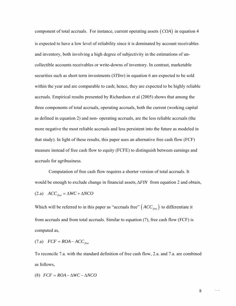
component of total accruals. For instance, current operating assets ( )COA in equation 4

is expected to have a low level of reliability since it is dominated by account receivables

and inventory, both involving a high degree of subjectivity in the estimations of un-

collectible accounts receivables or write-downs of inventory. In contrast, marketable

securities such as short term investments (STInv) in equation 6 are expected to be sold

within the year and are comparable to cash; hence, they are expected to be highly reliable

accruals. Empirical results presented by Richardson et al (2005) shows that among the

three components of total accruals, operating accruals, both the current (working capital

as defined in equation 2) and non- operating accruals, are the less reliable accruals (the

more negative the most reliable accruals and less persistent into the future as modeled in

that study). In light of these results, this paper uses an alternative free cash flow (FCF)

measure instead of free cash flow to equity (FCFE) to distinguish between earnings and

accruals for agribusiness.

Computation of free cash flow requires a shorter version of total accruals. It

would be enough to exclude change in financial assets, FIN∆ from equation 2 and obtain,

(2.a) freeACC WC NCO= ∆ + ∆

Which will be referred to in this paper as “accruals free” ( )freeACC to differentiate it

from accruals and from total accruals. Similar to equation (7), free cash flow (FCF) is

computed as,

(7.a) freeFCF ROA ACC= −

To reconcile 7.a. with the standard definition of free cash flow, 2.a. and 7.a. are combined

as follows,

(8) FCF ROA WC NCO= − ∆ − ∆

- - 8

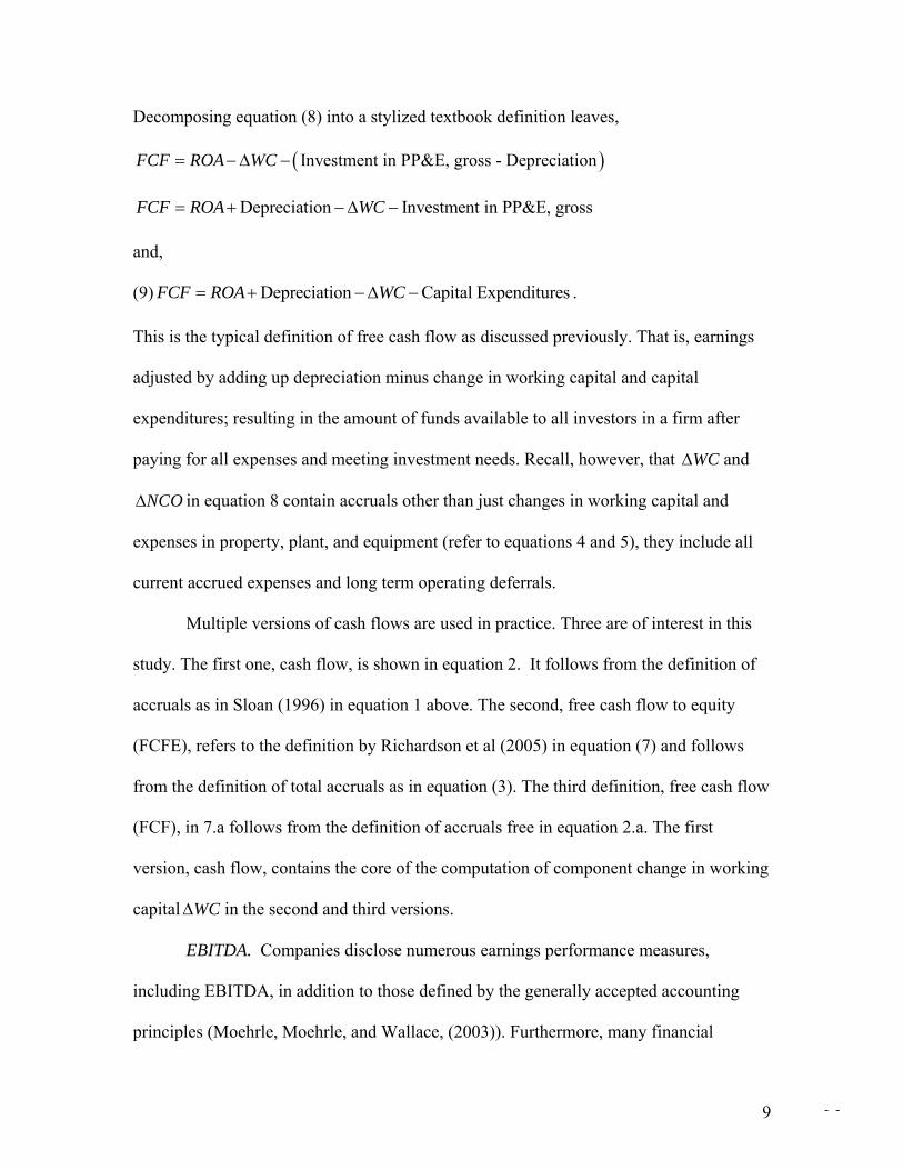
Decomposing equation (8) into a stylized textbook definition leaves,

( )Investment in PP&E, gross - DepreciationFCF ROA WC= − ∆ −

Depreciation Investment in PP&E, grossFCF ROA WC= + −∆ −

and,

(9) . Depreciation Capital ExpendituresFCF ROA WC= + −∆ −

This is the typical definition of free cash flow as discussed previously. That is, earnings

adjusted by adding up depreciation minus change in working capital and capital

expenditures; resulting in the amount of funds available to all investors in a firm after

paying for all expenses and meeting investment needs. Recall, however, that and

in equation 8 contain accruals other than just changes in working capital and

expenses in property, plant, and equipment (refer to equations 4 and 5), they include all

current accrued expenses and long term operating deferrals.

WC∆

NCO∆

Multiple versions of cash flows are used in practice. Three are of interest in this

study. The first one, cash flow, is shown in equation 2. It follows from the definition of

accruals as in Sloan (1996) in equation 1 above. The second, free cash flow to equity

(FCFE), refers to the definition by Richardson et al (2005) in equation (7) and follows

from the definition of total accruals as in equation (3). The third definition, free cash flow

(FCF), in 7.a follows from the definition of accruals free in equation 2.a. The first

version, cash flow, contains the core of the computation of component change in working

capital in the second and third versions. WC∆

EBITDA. Companies disclose numerous earnings performance measures,

including EBITDA, in addition to those defined by the generally accepted accounting

principles (Moehrle, Moehrle, and Wallace, (2003)). Furthermore, many financial

- - 9

analysts have widely adopted EBITDA as a proxy for cash flows of operations (Shook

(2003 )). EBITDA, however, as opposed to cash flows, excludes among other items

changes in working capital. Academics and practitioners have serious doubts about the

use of EBITDA as a proxy of cash flow from operations, arguing that EBITDA is often

misleading and does not accurately reflect liquidity or cash flow. To illustrate this

concern, some financial accounting considerations follow.

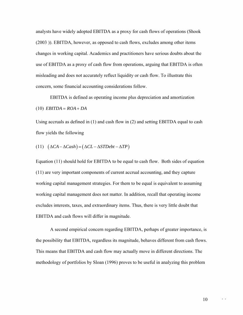
EBITDA is defined as operating income plus depreciation and amortization

(10) EBITDA ROA DA= +

Using accruals as defined in (1) and cash flow in (2) and setting EBITDA equal to cash

flow yields the following

(11) ( ) (CA Cash CL STDebt TP∆ −∆ = ∆ −∆ −∆ )

Equation (11) should hold for EBITDA to be equal to cash flow. Both sides of equation

(11) are very important components of current accrual accounting, and they capture

working capital management strategies. For them to be equal is equivalent to assuming

working capital management does not matter. In addition, recall that operating income

excludes interests, taxes, and extraordinary items. Thus, there is very little doubt that

EBITDA and cash flows will differ in magnitude.

A second empirical concern regarding EBITDA, perhaps of greater importance, is

the possibility that EBITDA, regardless its magnitude, behaves different from cash flows.

This means that EBITDA and cash flow may actually move in different directions. The

methodology of portfolios by Sloan (1996) proves to be useful in analyzing this problem

- - 10

since it allows for comparison of accruals and cash flow (and EBITDA in our problem)

across sections or portfolios with different accruals and cash magnitudes.

The use of EBITDA is suspicious given the fact that this measure uses earnings

and depreciation dollars earmarked for replacement capital. Based on this property, for

instance, Koller, Goedhart, and Wessels (2005) refer to EBITDA as a "good measure of

extremely low short-term ability to meet interest payments… most companies cannot

survive very long without replacing worn assets".

Why has EBITDA received much attention in corporate finance? Why not simply

use cash flows? Possible reasons include, 1) EBITDA involves less components than

cash flows making it easier to forecast, 2) EBITDA in general looks better since it tends

to be larger than the cash flows of operations, and 3) the statement of cash flow is still

considered the “new” statement and many managers are not as familiar with this

statement as they are with the other financial statements (Hertenstein and McKinnon

(1997)).

Results

Total Accruals and Free Cash Flows to Equity. Descriptive statistics for

agribusiness are presented in table 1 along with results from the previous study by

Richardson et al (2005) for all firms (excluding financial firms). The agribusiness sample

used in this study represents around 5% of the ‘all firms’ sample. From panel A table 1 it

can be observed that on average earnings for agribusiness firms is 10.6% of assets (with a

0.127 standard deviation) whereas for ‘all firms’ this figure is 7% (with a corresponding

0.175 standard deviation). Average total accruals (TACC) represents 3.5% of average

- - 11

total assets compared to 5.2% for ‘all firms’. In general, firms with higher positive

accruals are faster growing firms and require higher levels of cash flow to support their

growth. Agribusiness, as suggested by the results, is an above of average industry in

terms of profitability and free cash flow to equity.

Panel B of table 1 reports the decomposition of total accruals into its three main

elements, working capital (the current operating component), non-current operating

assets (the non-current operating and investing component), and net financial assets (the

financing component). It is evident that changes in non-current operating assets,

contributes the most to total accruals. Also, while the change in working capital and

change in non-current operating assets are positive, the change in net financial assets is

negative, supporting the idea developed in Richardson et al (2005) that the average firm

is growing its net operating assets and reducing its net financial assets (e.g. increasing its

net debt position) to finance this growth. In other words, the average firm is not internally

financing its growth.

NCO∆

Panel C of table 1 includes free cash flow to equity (FCFE) and EBITDA. These

two metrics along with ROA are commonly used in practice to measure firms’

performance. And as noted, many financial analysts have widely adopted EBITDA as a

proxy for cash flows of operations (Shook, 2003). EBITDA is by far the largest among

all those measures from table 1 (0.152 compared to 0.106 and 0.071). This result supports

the appeal of EBITDA to managers when providing performance measures to investors

and board of directors.

Table 2 presents the Pearson pair-wise correlations for total accruals

decomposition for agribusiness (bold, the upper right) and for ‘all firms’ (lower left).

- - 12

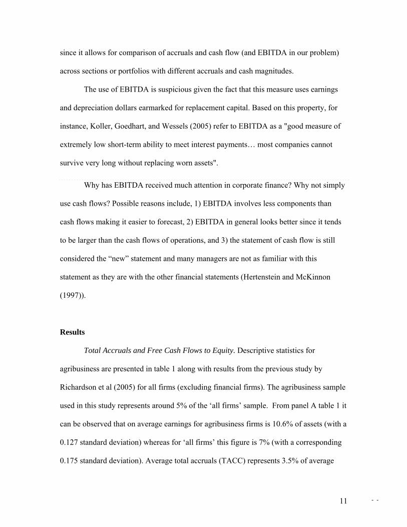
Positive correlation between current and non-current accruals (0.14 for agribusiness),

negative correlations between financial accruals and both current operating accruals (-0.4

for agribusiness) and non-current operating accruals (-0.63 for agribusiness) are

consistent with the ‘all firms’ correlations. This suggests that firms on average tend to

grow their current and non-current activities in tandem (Richardson et al (2005)) and tend

to finance such growth by reducing their net financial assets position either by reducing

their financial investments or by increasing financial liabilities. It can also be noticed

from the matrix that the positive correlation between change in financing accruals,

, and earnings in period t and t+1 is the same at the two decimal level for both

agribusiness and ‘all firms’ (0.11 and 0.04 respectively) suggesting the dominance of

long term over short term financing activities as related to earnings.

FIN∆

Correlations between each component of accruals and free cash flow to equity not

reported show that the correlation between current operating accruals and free cash flow

to equity, and between non- current operating accruals and free cash flow to equity are

higher than the correlation between financial accruals and free cash flow to equity. This

suggests the dominance of operating over financial accruals in explaining free cash flows.

Statistics from tables 1 and 2 are supportive of the following two ideas, a) the importance

of extending the classical definition of accruals as proposed by Richardson et al (2005),

and b) the agribusiness industry behaves in a manner that is similar to all other firms,

with regards to accruals and cash flows.

Total Accruals and Free Cash Flows to Equity across Portfolios. Previous

studies by Sloan (1996) and Dechow (1994) for ‘all firms’ traded on the U.S. stock

exchanges document a negative relationship between accruals and cash flows. Both

- - 13

studies use the definition of current accruals and follow the portfolios methodology.

Following Sloan (1996) firms are ranked by the magnitude of accruals every year and

five portfolios are formed based on quintiles. Means and medians of selected variables

are reported by portfolio, thus allowing for cross sectional comparisons. Portfolios for

agribusiness are formed but using the total accruals instead of accruals as done in Sloan

(1996). Additionally, EBITDA, a measure not included in previous research related to

accruals and cash flows, is included in this study. Panel A of Table 3 shows the

components of earnings and EBITDA, panel B shows a decomposition of total accruals,

and panel C presents depreciation and amortization.

As one moves from portfolio 1 to portfolio 5 (lowest total accruals with a mean

(median) of -0.11 (-0.05) to highest total accruals with a mean (median) of 0.18 (0.13))

free cash flow to equity, FCFE, decreases from a mean of 0.13 to -0.022. Free cash flow

to equity, however, remains stable for portfolios in the middle (portfolios 2, 3, and 4)

with values of 0.08, which is around the mean of 0.071 reported for FCFE in table 1. A

possible explanation to this is the existing difference in correlations among the

components of total accruals, as reported in table 2. The performance of earning across

portfolios is clearer. There is a strong positive relationship between total accruals

(TACC) and earnings (ROA). When agribusiness’ increase earnings the increment of

total accruals offsets the effects on cash and free cash flow to equity tends to decrease.

Agribusinesses reporting high positive total accruals are growing firms with more

potential to manipulate reported earnings increasing the distress on equity holders due to

2 When interpreting cash flows, keep in mind that cash flows computed using the accruals framework will tend to be higher than ‘actual’ cash flows figures taken directly from the statement of cash flows, mainly because operating income instead of net earnings is used as variable earnings as this presents some advantages discussed in the methodology section.

- - 14

the decrease in free cash flow to equity. EBITDA, however, shows the opposite. As

agribusiness increase total accruals EBITDA increases significantly from portfolio 1 with

a mean of 0.07 to the portfolio 5 with values of 0.20. This happens because of the strong

positive relationship between total accruals and earnings; since ROA is defined as

operating income after depreciation and amortization as total accruals (hence, ROA)

increases across portfolios EBITDA unambiguously increases also3. This result is

consistent with the view of EBITDA as a suspicious measure to evaluate firm

performance.

Agribusiness with high levels of accruals are growing firms that fund such growth

with externally generated flows leaving little room for free cash flow to equity. Very high

levels of total accruals leading to negative free cash flow to equity (-0.02 in table 3 for

portfolio 5), however, would probably be harmful for agribusiness owners since it might

be the result of creditors restricting funds to the company as perceived risk had probably

increased. The behavior of in panel B table 3 supports this. As one moves across

portfolios, become less negative (recall negative accruals imply inflows) with this

value switching to positive for portfolio 5, the portfolio with the highest level of accruals.

In any situation, however, stockholders’ concern increases as the agribusiness may face

the need to stop dividends and sale additional shares. An opposite plausible, but less

probable view is that the high growing company does not enter into distress and the

negative free cash flow is the result of the desire of stockholder to increase their position

in the company for capital structure reasons. Table 3, however, shows that EBITDA does

FIN∆

FIN∆

3 Alternative results not reported were obtained using net income and income before extraordinary items as variable earnings instead of operating income after depreciation and amortization. Quality of results is similar.

- - 15

not capture this effect. Using EBITDA as a proxy for cash flow would be misleading in

such a situation.

In panel B of table 3 a decomposition of total accruals is shown. All components

seem to have a regular behavior when analyzed across portfolios. Consistent with results

from table 1, the components andFIN∆ NCO∆ taken together account for a higher

magnitude in total accruals than the WC∆ component. Recall that the former are the new

components aggregated to the classical definition of accruals.

Panel C of table 3 presents depreciation, which is the difference between

EBITDA and operating income after depreciation and amortization. Note that

depreciation & amortization for agribusiness remain stable around 5% with respect to

total assets regardless of the level of accruals firms report. Results by Sloan (1996) for

‘all firms’ are slightly different showing that as firms report higher component accruals

depreciation decreases from 6% in the ‘lowest’ portfolio to 3% in the ‘highest’. Although

in Sloan (1996) accruals measure is used instead of total accrual, our results, not reported,

for total accruals and for accrual free show the same stability around 5% of depreciation.

One should expect less variation in depreciation & amortization when analyzing firms

within an industry (i.e. agribusiness) than when all industries are pooled together (‘all

firms’) due to similarities in the nature of the assets structure of an industry. However,

significant variations within an industry across portfolios might exist due to the fact that

managers have discretion in some inputs that determine the amount to be depreciated

(such as estimation of residual values or useful life of PP&E), in such a scenario, one

should expect that aggressive firms with higher level of accruals to report lower

- - 16

depreciation values in order to show better earnings. This is not the case for agribusiness

industry on average as suggested by results on panel C table 3.

Accruals and Cash Flows across Portfolios. The previous analysis shows the

relationship between earnings and its components for agribusiness using total accruals as

proposed by Richardson et al (2005) but following the methodology by Sloan (1996) with

an extension for EBITDA. EBITDA is more closely related to cash flow from operations

than to free cash flow to equity. Results for agribusinesses presented in table 4 show

more clearly the negative relation between accruals (ACC) and cash flows (CF). As one

moves across portfolios and accruals increase from a mean of -0.04, 0.03, 0.06, 0.09, and

0.17, cash flows decrease from 0.10, 0.08, 0.06, 0.04, and -0.07. These are very similar

results to those for Sloan’s (1996) ‘all firms’. In this model there is not a plateau as the

one observed in free cash flow to equity in table 3 for portfolios 2, 3, and 4. Notice that

for portfolio 3, in the middle, agribusiness report a 12% ROA with equally distributed

accrual and cash flow components of 6%.

For EBITDA, its mean value is higher than cash flow’s (CF) for portfolio 2 to

portfolio 5. Note the differences between these two measures in “EBITDA-CF” in table

4. An agribusiness reporting 0.17 positive accruals in portfolio 5 (highest level of

accruals) would be experiencing negative cash flow from operations consistent with the

idea developed previously but will be reporting a high EBITDA of positive 0.16. In

addition, only agribusiness with negative or very low levels of accruals have ‘regular’

EBITDA’s but in such companies the distinction between cash and its shortcuts would

not be an issue in the absence of accruals earnings equal cash flows. Only in portfolio 1 is

EBITDA lower than cash flow from operations with a mean of 0.09 compared to 0.10.

- - 17

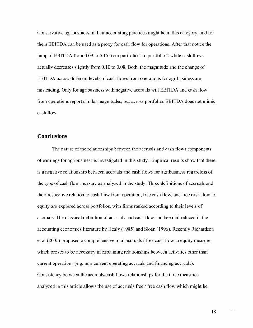
Conservative agribusiness in their accounting practices might be in this category, and for

them EBITDA can be used as a proxy for cash flow for operations. After that notice the

jump of EBITDA from 0.09 to 0.16 from portfolio 1 to portfolio 2 while cash flows

actually decreases slightly from 0.10 to 0.08. Both, the magnitude and the change of

EBITDA across different levels of cash flows from operations for agribusiness are

misleading. Only for agribusiness with negative accruals will EBITDA and cash flow

from operations report similar magnitudes, but across portfolios EBITDA does not mimic

cash flow.

Conclusions

The nature of the relationships between the accruals and cash flows components

of earnings for agribusiness is investigated in this study. Empirical results show that there

is a negative relationship between accruals and cash flows for agribusiness regardless of

the type of cash flow measure as analyzed in the study. Three definitions of accruals and

their respective relation to cash flow from operation, free cash flow, and free cash flow to

equity are explored across portfolios, with firms ranked according to their levels of

accruals. The classical definition of accruals and cash flow had been introduced in the

accounting economics literature by Healy (1985) and Sloan (1996). Recently Richardson

et al (2005) proposed a comprehensive total accruals / free cash flow to equity measure

which proves to be necessary in explaining relationships between activities other than

current operations (e.g. non-current operating accruals and financing accruals).

Consistency between the accruals/cash flows relationships for the three measures

analyzed in this article allows the use of accruals free / free cash flow which might be

- - 18

more suitable for agribusiness decision makers familiar with the free cash flows

framework.

EBITDA is also tested in this study as a potential metric to mimic cash flows.

Empirical results show that both the magnitudes and the behavior of EBITDA

significantly differs from cash flows for agribusiness. EBITDA, in most of the cases is

misleading. At best EBITDA might be used as a proxy for cash flows only for

agribusiness with conservative accounting practices.

Special attention with regards to cash flows should be taken for agribusinesses

reporting high levels of earnings since they tend to have high level of accruals.

Agribusiness with high level of accruals show very low levels of free cash flow which

might be harmful for debt and equity holders.

In comparison to ‘all firms’ the agribusiness industry behaves in a manner that is

similar with regards to accruals and cash flows. Result, however, suggest that the

agribusiness industry is an above average industry in terms of profitability and free cash

flows but not in terms of cash flow from operations. This suggests the need to further

explore the subcomponents of non-current operating accruals.

Results using accruals free and free cash flow lead to the same conclusions

discussed in this study. The two components of more importance for accruals to explain

the accruals/cash flows relationships for agribusiness are both the current operating

accruals and non-current operating accruals, which is useful for agribusiness decision

makers familiarized with free cash flow. Future research may further explore these two

components and subcomponents in terms of level of persistence into the future, and in

terms of their relationship with categorized metrics such as financial ratios (e.g. quality of

- - 19

ratios) used in agribusiness to measure financial performance. The introduction of risk

and return on these models may also be of interest for future work.

- - 20

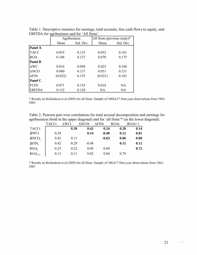
Table 1. Descriptive statistics for earnings, total accruals, free cash flows to equity, and EBITDA for agribusiness and for ‘All firms’.

Mean Std. Dev. Mean Std. Dev.Panel ATACC 0.035 0.133 0.052 0.181ROA 0.106 0.127 0.070 0.175Panel B∆WC 0.016 0.094 0.022 0.108∆NCO 0.040 0.137 0.051 0.151∆FIN (0.022) 0.153 (0.021) 0.181Panel CFCFE 0.071 0.155 0.018 NAEBITDA 0.152 0.128 NA NA

All firms (previous study)*Agribusiness

* Results on Richardson et al (2005) for all firms. Sample of 1088,617 firm-year observations from 1962-2001. Table 2. Pearson pair-wise correlations for total accrual decomposition and earnings for agribusiness (bold in the upper diagonal) and for ‘all firms’* (in the lower diagonal).

TACCt ∆WCt ∆NCOt ∆FINt ROAt ROAt+1TACCt 0.39 0.42 0.24 0.28 0.14∆WCt 0.39 0.14 -0.40 0.12 0.01∆NCOt 0.42 0.11 -0.63 0.06 0.00∆FINt 0.42 -0.29 -0.48 0.11 0.11ROAt 0.25 0.22 0.09 0.04 0.72ROAt+1 0.13 0.11 0.02 0.04 0.79

* Results on Richardson et al (2005) for all firms. Sample of 108,617 firm-year observations from 1962-2001

- - 21

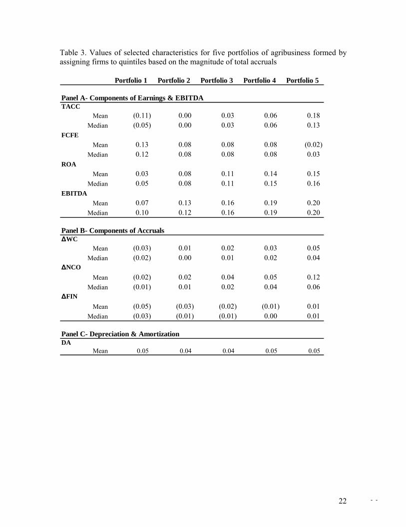
Table 3. Values of selected characteristics for five portfolios of agribusiness formed by assigning firms to quintiles based on the magnitude of total accruals

Portfolio 1 Portfolio 2 Portfolio 3 Portfolio 4 Portfolio 5

Panel A- Components of Earnings & EBITDATACC

Mean (0.11) 0.00 0.03 0.06 0.18Median (0.05) 0.00 0.03 0.06 0.13

FCFEMean 0.13 0.08 0.08 0.08 (0.02)

Median 0.12 0.08 0.08 0.08 0.03ROA

Mean 0.03 0.08 0.11 0.14 0.15Median 0.05 0.08 0.11 0.15 0.16

EBITDAMean 0.07 0.13 0.16 0.19 0.20

Median 0.10 0.12 0.16 0.19 0.20

Panel B- Components of Accruals∆WC

Mean (0.03) 0.01 0.02 0.03 0.05Median (0.02) 0.00 0.01 0.02 0.04

∆NCOMean (0.02) 0.02 0.04 0.05 0.12

Median (0.01) 0.01 0.02 0.04 0.06∆FIN

Mean (0.05) (0.03) (0.02) (0.01) 0.01Median (0.03) (0.01) (0.01) 0.00 0.01

Panel C- Depreciation & AmortizationDA

Mean 0.05 0.04 0.04 0.05 0.05

- - 22

Table 4. Mean of selected characteristics for five portfolios of agribusiness formed by assigning firms to quintiles based on the magnitude of total accruals.

Portfolio 1 Portfolio 2 Portfolio 3 Portfolio 4 Portfolio 5

ACC (0.04) 0.03 0.06 0.09 0.17CF 0.10 0.08 0.06 0.04 (0.07)ROA 0.06 0.12 0.12 0.13 0.11EBITDA 0.09 0.16 0.17 0.18 0.16EBITDA-CF (0.01) 0.08 0.11 0.14 0.23 References

Beaver, W. "The Time Series Behavior of Earnings." Journal of Accounting Research

(1970): 62-99. Brigham, E., and M. Ehrhardt. Financial Management Theory and Practice. 11th ed:

Thomson South Western, 2005. Dechow, P. "Accounting Earning and Cash Flows as Measures of Firm Performance. The

Role of Accounting Accruals " Journal of Accounting and Economics 18(1994): 3-42.

Fama, E., and K. French. "The Cross-Section of Expected Stock Returns." The Journal of Finance XLVII no. No. 2(1992): 427-465.

Freeman, R., J. Ohlson, and S. Penman. "Book-rate-of-return and Prediction of Earnings Changes: An Empirical Investigation." Journal of Accounting Research 20(1982): 639-653.

Greenwood, R., and D. Sharchfstein. "Calculating Free Cash Flows." Harvard Business School, no. 9-206-028(2005).

Healy, P. M. "The effect of bonus schemes on accounting decisions." Journal of Accounting and Economics 7, no. 1-3(1985): 85-107.

Hertenstein, J., and S. McKinnon. "Solving the Puzzle of the Cash Flow Statement." Harvard Business School Publishing, Business Horizons BH013(1997 ).

Hough, J. (2005) Free Cash Flow. Koller, T., M. Goedhart, and D. Wessels. Measuring and Managing the Value of

Companies. 4th ed. Hoboken, New Jersey: John Wiley & Sons, Inc., 2005. Moehrle, S., J. Reynolds- Moehrle, and J. Wallace. " Dining at the Earnings Buffet."

Harvard Business School Publishing - Business Horizons. Richardson, S. A., et al. "Accrual reliability, earnings persistence and stock prices."

Journal of Accounting and Economics 39, no. 3(2005): 437-485. Shook, D. "EBITDA’s Foggy Bottom Line." Business Week, January 14, 2003. Sloan, R. G. "Do Stock Prices Fully Reflect Information in Accruals and Cash Flows

About Future Earnings?" Accounting Review Vol. 71 no. Issue 3(1996): p289-315.

- - 23