Master’s thesis accounting, auditing and control 

Equity incentives and earnings management  In partial fulfillment of the requirements for the degree of Master of Science in Economics and Business     Erasmus University Rotterdam Department:   Business Economics Section:    Accounting, Auditing & Control Course code:  FEM 11032‐11 Supervisor:    Dr. C.D. Knoops Written by:    Winfred Damler Student nr:    295272 Date:      July 2012 

2

Abstract This  master’s  thesis  examines  the  relation  between  equity  incentives  and  earnings 

management.  It  extends  prior  research  by  providing  a  more  detailed  insight  on  the 

relation between discretionary accruals and equity incentives. The study finds evidence 

for a  significant  relation between discretionary accruals  calculated by a  linear Kothari 

accrual model and equity incentives, in a pre‐Sarbanes Oxley sample. It shows that this 

relation is stronger for CFO equity incentives than for CEO equity incentives. The study 

finds  a  significant  positive  relation  between  earnings  management  and  total  equity 

incentives; it also shows such a positive relation for option‐based equity incentives. For 

stock‐based equity incentives no such positive relation is found. The third finding is that 

the  relation  between  earnings management  and  equity  incentives  changes  before  and 

after the major accounting scandals and introduction of the Sarbanes Oxley act.  

Abbreviations  CEO            Chief executive officer CFO            Chief financial officer GAAP            Generally accepted accounting principles IRS            Internal revenue service M&A            Mergers and acquisitions ROA            Return on assets R&D            Research and Development SEC            Securities and Exchange Commission SIC            Standard industry classification SOX            Sarbanes Oxley act US            United States of America 

 

3

Table of Contents ABSTRACT ........................................................................................................................................................... 2 ABBREVIATIONS ............................................................................................................................................... 2 CHAPTER 1 INTRODUCTION ........................................................................................................................ 5 1.1 INTRODUCTION ........................................................................................................................................................... 5 1.2 PURPOSE OF THE THESIS AND RESEARCH QUESTION ............................................................................................ 8 1.3 RELEVANCE AND CONTRIBUTION ............................................................................................................................ 9 1.4 STRUCTURE OF THE THESIS .................................................................................................................................... 10 

CHAPTER 2 EARNINGS MANAGEMENT, THE THEORY ...................................................................... 11 2.1 INTRODUCTION AND THE REASON FOR EARNINGS MANAGEMENT ................................................................... 11 2.2 WHAT DO WE CONSIDER EARNINGS MANAGEMENT? ......................................................................................... 13 2.3 MEASURING EARNINGS MANAGEMENT WITH ACCRUALS ................................................................................... 17 2.4 WHO COMMITS EARNINGS MANAGEMENT? ......................................................................................................... 18 2.5 SUMMARY DEFINITION EARNINGS MANAGEMENT .............................................................................................. 18 

CHAPTER 3 ACCRUAL MODELS ................................................................................................................. 20 3.1 ACCRUALS .................................................................................................................................................................. 20 3.2 THE HEALY MODEL 1985 ....................................................................................................................................... 22 3.3 THE DE ANGELO MODEL 1986 .............................................................................................................................. 23 3.4 JONES MODEL 1991 ................................................................................................................................................. 23 3.5 MODIFIED JONES MODEL 1995 ............................................................................................................................. 26 3.6 TIME‐SERIES VERSUS CROSS SECTIONAL JONES MODELS ................................................................................... 27 3.6.1 Time‐Series designs with the Jones model .................................................................................................28 3.6.2 Cross‐sectional designs with the Jones model ..........................................................................................29 

3.7 DIFFERENCE BETWEEN BALANCE SHEET ACCRUALS AND CASH FLOW ACCRUALS ......................................... 30 3.8 IMPROVED VERSIONS OF THE JONES MODEL ........................................................................................................ 32 3.9 THE FORWARD‐LOOKING MODEL 2003 ............................................................................................................... 32 3.10 CASH FLOW JONES MODEL 2002 ........................................................................................................................ 34 3.11 LARCKER AND RICHARDSON 2004 .................................................................................................................... 37 3.12 PERFORMANCE MATCHING MODEL 2005 ......................................................................................................... 38 3.13 THE BUSINESS MODEL 2007 .............................................................................................................................. 41 3.14 RECENT LITERATURE ON ACCRUAL MODELS ..................................................................................................... 44 3.15 CHAPTER 3 SUMMARY........................................................................................................................................... 45 

CHAPTER 4 ESTIMATING THE EQUITY INCENTIVES ......................................................................... 47 4.1 BOUNDARIES OF BONUS SCHEMES.......................................................................................................................... 47 4.2 MAXIMIZING EARNINGS IN JAPAN .......................................................................................................................... 47 4.3 PROXY FOR EQUITY INCENTIVES ............................................................................................................................ 48 4.4 SUMMARY .................................................................................................................................................................. 49 

CHAPTER 5 EMPIRICAL RESEARCH ON EARNINGS MANAGEMENT DUE TO EQUITY INCENTIVES ..................................................................................................................................................... 50 5.1  INTRODUCTION ........................................................................................................................................................ 50 5.2 REMUNERATION ....................................................................................................................................................... 50 5.3 EQUITY INCENTIVES ................................................................................................................................................. 54 5.4 CEO AND CFO EQUITY INCENTIVES ...................................................................................................................... 59 5.5 SUMMARY .................................................................................................................................................................. 64 

CHAPTER 6 HYPOTHESIS ............................................................................................................................ 66 6.1 HYPOTHESIS 1 .......................................................................................................................................................... 66 6.2 HYPOTHESIS 2 .......................................................................................................................................................... 66 

4

6.3 HYPOTHESIS 3 .......................................................................................................................................................... 66 6.4 HYPOTHESIS 4 .......................................................................................................................................................... 67 

CHAPTER 7 RESEARCH DESIGN AND METHODOLOGY ..................................................................... 69 7.1 INTRODUCTION ......................................................................................................................................................... 69 7.2 ACCRUAL MODEL ...................................................................................................................................................... 69 7.3 MEASURE FOR EQUITY INCENTIVES ....................................................................................................................... 71 7.4 ESTIMATING THE RELATION BETWEEN EARNINGS MANAGEMENT AND EQUITY INCENTIVES ..................... 73 7.5 SAMPLE ...................................................................................................................................................................... 73 7.6 DESCRIPTIVE STATISTICS ........................................................................................................................................ 74 

CHAPTER 8 FINDINGS .................................................................................................................................. 79 8.1 INTRODUCTION ......................................................................................................................................................... 79 8.2 HYPOTHESIS 1 .......................................................................................................................................................... 82 8.3 HYPOTHESIS 2 .......................................................................................................................................................... 83 8.4 HYPOTHESIS 3 .......................................................................................................................................................... 85 8.5 HYPOTHESIS 4 .......................................................................................................................................................... 86 8.6 SUMMARY .................................................................................................................................................................. 88 

CHAPTER 9 LIMITATIONS .......................................................................................................................... 90 CHAPTER 10 CONCLUSION ......................................................................................................................... 93 SUMMARY AND MAIN CONCLUSIONS ............................................................................................................................. 93 RECOMMENDATIONS ....................................................................................................................................................... 93 

BIBLIOGRAPHY .............................................................................................................................................. 95 APPENDIX 1 ..................................................................................................................................................... 97 APPENDIX 2 ..................................................................................................................................................... 99 APPENDIX 3 ...................................................................................................................................................100 APPENDIX 4 ...................................................................................................................................................101 

5

Chapter 1 introduction 

1.1 Introduction Management  compensation  has  been  a  much‐discussed  item  over  the  last  decade. 

Different  accounting  scandals,  like  Enron,  Ahold  and  Parmalat  have  damaged  trust  in 

executive managers and financial reports. Due to these scandals, there has been a lot of 

discussion about remuneration of executives. Stock and option‐based compensation has 

increased  strongly  during  the  1980’s  and  the  1990’s  (Bergstresser & Philippon, 2006). 

Before that time managers had little or no incentive to maximize the firms performance. 

Since that time the use of equity incentives has increased for a number of reasons. The 

most  obvious  reason  is  to  align  the  interests  of  the  owners  and  the  managers  of 

companies. Because interests of managers deviated from the interests of the owners of 

firms, firms were not effectively managed from an owner’s point of view. An example of 

this management behavior that is not line with owner’s interests is the fruitless “empire‐

building” as described  in the study by  Jensen  (1991);  too many mergers and takeovers 

led  to  large  firms,  instead  of  enhancing  performance  this  led  to  declining  corporate 

efficiency and destroying value.  

Until  the  1980’s  not  much  performance  enhancing  incentives  were  provided  to 

management, this led to behavior from managers that was not in line with the interests 

of stockholders. To provide management with an incentive to increase firm performance 

companies  started  using  more  equity‐based  incentives.  Mehran’s  (1995)  study 

demonstrates  that  providing  performance  enhancing  incentives  can  work;  his  study 

shows  that  firm  performance  is  enhanced  by  providing  management  with  stock  or 

option‐based  compensation.  Not  only  equity‐based  incentives  were  introduced, 

performance related bonuses where introduced as well. While the purpose of stock and 

option‐based  compensation  plans  was  to  align  the  interest  of  management  with  the 

interests  of  the  owners  of  the  company,  this  also  opened  the  door  to  opportunistic 

behavior from management, as they could influence their remuneration by maximizing 

the performance of  the company. Healy  (1985)  is one of  the  first  to provide proof  that 

managers use earnings management techniques to maximize their income.  

6

Due  to accounting scandals  rewarding executives with equity  incentives has become a 

much‐discussed  topic.  For  this  discussion  it  is  important  to  know what  the  effects  of 

equity  incentives are, and how the  relation between earnings management and equity 

incentives works. This master’s thesis examines this relation for a sample of large firms 

that are listed in the United States and are part of the S&P 500. 

A  first  aspect  this  master’s  thesis  focuses  on  is  the  difference  between  CEO  and  CFO 

equity incentives. Much of the prior research on this subject has focused on the relation 

between the total equity incentives rewarded to the CEO and earnings management. But 

there is more in it than just that. It is very well possible that the CFO has more influence 

on accounting and accrual decisions than the CEO. As the CFO is the one responsible for 

the  financial  administration  of  the  firm  and  he  is  the  one  in  charge  of  composing  the 

financial  statements.    Therefore  it  is  useful  to  examine  the  relation  between  equity 

incentives  and  earnings  management  for  both  the  CEO  and  the  CFO  as  it  might  be 

possible that awarding equity incentives to the CFO, who is responsible for the financial 

statements leads to more earnings management than equity incentives awarded to the 

CEO, as the CEO cannot influence the financial statements as directly as the CFO can.  

A  second  aspect  this  study  examines  is  the  effects  of  the  different  kinds  of  equity 

incentives. Executives can be rewarded with different equity incentives, it is likely that 

these  different  incentives  have  different  effects  on  the  behavior  of  the  executives 

because the characteristics of the equity incentives differ. There are more remuneration 

incentives  that  can  have  an  influence  on  management  behavior  like  bonuses;  this 

master’s  thesis will  be  limited  to  equity  incentives.  Equity  incentives  can be based on 

stocks or derivates from stock,  like options. This master’s thesis focuses on share‐ and 

option‐based  incentives.  An  important  characteristic  of  options  is  that  most  options 

have  an  expiration  date,  after  this  date  the  option  has  no  value  anymore.  As  a  result 

options  are  relatively  short  time  incentives.  Options  motivate  managers  to  increase 

earnings until  the expiration date of  the options. Due  to  this,  option  incentives are by 

definition  incentives  to  increase  short‐term  firm  performance.  Stock‐based  incentives 

have  no  expiration  date;  a  manager  can  benefit  from  both  short‐  and  long‐term  firm 

performance.    As  stocks  do  not  have  an  expiration  data  they  are  a  more  permanent 

incentive  than  options,  the  incentive  only  ends  if  the  shares  are  sold.  Another 

characteristic of options is that executives can benefit from an increase in the stock price 

7

due to earnings management, but that his wealth does not suffer much if the stock price 

declines (Burns & Kedia, 2006). Therefore option‐based incentives can lead to managers 

taking more  risk  and  to  use  earnings management,  as  their wealth  is  not  affected  so 

much if things go wrong. This is different for share‐based incentives.  

A  third  aspect  this  study  looks  into  is  the  change  over  time  of  the  relation  between 

equity incentives and earnings management. Scandals like Enron and Ahold at the start 

of the last decade have led to heaps of public attention on management compensation; 

this might have led to companies changing their remuneration policies in order to keep 

their  reputation  intact. Another reaction  is  that  the  scandals have  led  to  legislation on 

reporting  details  of management  compensation.  An  example  of  such  legislation  is  the 

Sarbanes Oxley act in 2002. Some of the managers involved in accounting scandals have 

been convicted,  this  in combination with new legislation and more public attention on 

the subject may have led to a situation where managers are more careful to use earnings 

management. They are more in the spotlight these days and are possibly more aware of 

the  consequences  of  earnings  management.  I  examine  the  relation  between  earnings 

management and equity incentives over a 10 years period. Starting in 1999, two years 

before the major accounting scandals, until 2009. It  is useful to examine if the relation 

between earnings management and equity incentives changes over time, as it indicates 

the  effect  changes  following  the  accounting  scandals  have  had.  It  is  possible  that 

companies use different forms of remuneration nowadays, for instance more long‐term 

incentives.  This change in equity incentives is probably due to the accounting scandals 

of  the  early  2000’s.  In  the 1980’s  and 1990’s  option‐based  equity  incentives were  the 

most  important  equity  incentives,  I  expect  however  that  the  use  of  options  as  equity 

incentives  has  declined  and  that  share‐based  equity  incentives  are  more  important 

nowadays. This expectation is supported by the Global Equity incentives survey by PWC

(2011). This survey shows that performance‐based shares and share units are now more 

used  than  stock  options.  It  could  also  be  the  fact  that  managers  do  not  want  to  use 

earnings management too much anymore as they are afraid for the consequences.  It  is 

useful  to  see  if  and  how managers  and  firms  reacted  to  the  changed  situation  or  that 

there  is  not  much  difference  between  1999  and  2009  despite  all  the  changes  in  the 

environment. 

8

1.2 Purpose of the thesis and research question This master’s  thesis  examines  the  relation  between  earnings management  and  equity 

incentives. I  intend to more precisely examine if this relation is different for incentives 

awarded to the CEO and the CFO and if there are different effects for option‐ and stock‐

based  equity  incentives.  I  examine  this  relation  over  a  ten‐year  period  (1999‐2009) 

covering  major  accounting  scandals,  the  years  preceding  these  scandals  and  the 

aftermath of those scandals. This leads to a more detailed insight on the effect of equity 

incentives  and  provides  information  on  the  effect  of  measures  taken  in  response  to 

accounting  scandals  on  the  relation  between  earnings  management  and  equity 

incentives.  

My main research question is: 

What  is  the  relation  between  earnings  management  and  equity  incentives  awarded  to 

CEO’s and CFO’s?  

To analyze this relation further I examine the following sub questions: 

‐ Is  this  relation  different  for  incentives  awarded  to  a  CFO  than  for  incentives 

awarded to a CEO? 

‐ Does this relation defer for stock or option‐based incentives?  

‐ Do these relations change in the 10 years period from 1999 to 2009? 

The  goal  of  this  master’s  thesis  is  to  provide  more  detailed  insight  in  the  relation 

between  earnings  management  and  equity  incentives.  By  answering  these  research 

questions  I  provide  insight  in  the  difference  in  the  relation  between  earnings 

management  and  equity  incentives  for  the  CEO  and  the  CFO.  Much  of  the  previous 

research has  focused on  this  relation  for  the CEO only, while  this  relation  for  the CFO 

might even be stronger.  One can imagine that the CFO has a big influence on accounting 

decisions. As the CFO is responsible for the financial statements it might not be a good 

idea  that  his  personal  wealth  depends  on  the  earnings  of  the  company.  Because  the 

financial administration  is  the responsibility of  the CFO it could be  that  the CFO is  the 

manager who takes most of the accounting decisions. Therefore it could be the fact that 

equity  incentives  for CFO’s  have more  influence on earnings management  than equity 

incentives  for  CEO’s.  One  could  argue  that  it  would  be  wise  to  have  a  CFO  whose 

9

personal wealth does not depend on firm performance. Especially  in a situation where 

the CEO’s remuneration does depend on the performance of the company this could be 

important.  The  financially  independent  CFO  can  in  such  a  situation  prevent  the  CEO 

from opportunistic behavior. This master’s thesis examines if there is a positive relation 

between earnings management and equity incentives for the CFO and if this relation is 

stronger or weaker than the relation of the CEO.  

As mentioned in the previous section stock and option‐based equity incentives may have 

a  different  effect  than  share‐based  incentives.  Because  option‐based  incentives  are 

expected  to  provide  a  short‐term  incentive  due  to  the  expiration  date  of  the  options 

while the incentive for stock‐based remuneration has a more long‐term effect as stocks 

do not have such an expiration date.  

The  third  sub  question  focuses  on  the  change  of  this  relation  over  time;  it  provides 

information  if  the  relations  described  above  have  changed  over  the  years  and  if  the 

measures taken in the aftermath of accounting scandals had an effect on these relations. 

For  this  I  examine a  sample of  companies  that are part of  the S&P 500 as  the needed 

data is available for these companies in the “compustat” database. I use an accrual model 

to measure earnings management and compare this accrual model with the dependence 

of a manager’s income on the stock price. This master’s thesis contains a literature study 

that  covers  prior  research  on measuring  earnings management  and  equity  incentives 

and it contains an empirical research to answer the research question.  

1.3 Relevance and contribution This master’s  thesis  contributes  to  the  field  of  research  because  it  provides  a  more 

specified  insight  in  the  relation  between  equity  incentives  and  earnings management. 

Where  much  of  the  prior  research  focused  on  the  role  of  the  CEO  and  at  equity 

incentives as a whole, this master’s thesis examines the role of the CEO and the CFO and 

examines  whether  short‐term  option‐based  incentives  have  different  effects  on  the 

behavior of management than stock‐based incentives.  

The second point why this master’s thesis is relevant is that it helps understanding the 

relations  between  equity  incentives  and  earnings  management  in  more  detail.  This 

makes it possible to provide managers in the future with adequate remuneration plans 

that will maximize  their  productivity  but  do  not  create  an  incentive  for  opportunistic 

10

behavior. It provides knowledge needed, not only to create better future remuneration 

plans  but  also  to  provide  information  that  is  useful  in  the  discussion  around 

management remuneration and creating legislation on management remuneration. 

This master’s thesis also provides insight in the question if the relation between equity 

incentives and earnings management has  changed due  to accounting  scandals and  the 

measures taken  in the aftermath of  these scandals.  It shows whether the scandals and 

the measures taken after these scandals have changed the effect of equity incentives and 

it will show if this is different for short‐term option‐based incentives and for the more 

long‐term stock‐based  incentives.  It helps to analyze the effect of  legislation and other 

measures taken considering management remuneration. 

1.4 Structure of the thesis To  examine  the  subject  and  to  find  an  answer  to  the  research  question  this master’s 

thesis  proceeds  as  follows:  Chapter  two  discusses what  earnings management  entails 

and why  it  can be  triggered by equity  incentives. Chapter  three and  four describe  the 

literature on measuring earnings management with accruals accounting and measuring 

equity  incentives  respectively.  Chapter  five  presents  the  hypotheses  for  the  empirical 

part  of  the master’s  thesis,  chapter  six  discusses  the  methodology  and  the  research 

design  and  the  sample  used.  Chapter  seven  presents  the  results  of  the  empirical 

research  and  chapter  eight discusses  the  limitations  of  the  research.  The  last  chapter, 

chapter  nine,  presents  the  conclusions,  a  summary  and  recommendations  for  further 

research.  

11

Chapter 2 earnings management, the theory  

2.1 introduction and the reason for earnings management In  this  chapter  I  discuss:  what  earnings management  is,  why  it  exists,  how  it  can  be 

measured and who uses earnings management. In this master’s thesis I look at earnings 

management by board members. To understand the idea of earnings management it  is 

important to know why people take the effort to manage these earnings.  

A well‐known  theory on decision‐making  is  the utility maximizing  theory. This  theory 

was designed in the 18th and 19th century by Jeremey Benthem (1789) and John Steward 

Mill  (1863).  It  says  that  society  has  as  ultimate  goal  to  maximize  the  utility  of  all 

individual members of society.  Individual members of society will maximize their own 

utility; therefore a manager also looks to maximize his own utility. How the utility of a 

manager is maximized will differ from person to person.  

For a manager of a company who is trying to maximize his utility different factors might 

be  important,  for  instance: his social  status,  the  fact  that he wants  to keep his  job, his 

remuneration and the amount of effort he has to put in his job. For these factors other 

underlying  factors might be  important: For his  social  status  it might be  important  the 

company does well or that the press writes positive articles about the company. For his 

remuneration  it might  be  important  the  company  is  profitable  or  that  the  stock  price 

rises.  

Another  theory  that  comes  into  play  is  the  ‘Agency  Theory’  originally  introduced  by 

Adam  Smith  (Smith, 1776).  This  thesis  considers  publicly  held  companies,  in  those 

companies there is a possible difference in interest between the owners of the company 

and  the  managers.  In  a  publicly  held  company  the  owner,  or  owners,  are  the 

stockholders.  I  assume  that  in  a  publicly  held  company  it  are  the managers who  take 

most of the decisions. Because the managers and the owners are often different people 

there can be a difference of interest between he manager (the agent) and the owner (the 

principal). Both want  to maximize  their personal utility,  but  as  their  interests  are not 

always in line this can lead to difficulties. Because the utility maximizing manager does 

not what  the  owners  of  the  company, who hire  the manager, want  him  to  do.  This  is 

called the principal agent dilemma (Jensen & Meckling, 1976). One of the solutions used 

12

to mitigate  this problem is  to  try to align the interest of  the principal and the agent. A 

common  way  to  do  this  is  to  provide  management  with  stock  and  option‐based 

remuneration.1 Thereby a part of their remuneration depends on the performance of the 

company on the stock markets. This brings the interests of the management more in line 

with  the  interest  of  the  owners  of  the  company,  who  are  also  dependent  on  the 

performance on the stock marked. The idea is that a manger whose interests are in line 

with the interests of the owner of the company makes decisions that are beneficial from 

the owners’ point of view.  In this situation maximizing stock value or paying dividends 

is now favorable for both managers and owners.  

In  this  master’s  thesis  I  look  at  managers  who,  as  I  assume,  want  to  maximize  their 

remuneration. In line with Healy’s earnings maximizing hypothesis (Healy, The effect of

bonus schemes on accounting decisions, 1985).  A manager will  try  to maximize his  own 

wealth despite possible negative effects for the company. We look at the case where the 

remuneration depends for a certain amount on the stock price of  the company.  In  this 

master’s thesis I focus on equity‐based remuneration in the form of stocks and options. 

There are however other ways to bring managers interest more in line with that of the 

owner  of  the  company,  for  instance  bonuses  that  depend  on  the  performance  of  the 

company or on the relative performance of the company in a peer group.  

A  manager  who  wants  to  maximize  his  remuneration  will,  if  the  height  of  his 

remuneration correlates strongly with the stock price, try to maximize the stock price. 

As I assume the stock price depends on the performance of the company, as earnings are 

an important indicator for the company’s performance the manager will try to maximize 

the  earnings,  because  this  is  in  line  with  his  interest2.  He  maximizes  his  utility  by 

maximizing the company’s stock price. Mehran (1995) finds that this actually works. He 

finds  that:  “firm  performance  is  positively  related  to  the  share  of  equity  held  by 

managers, and the share of management compensation that is equity‐based”.  

On  the other hand  if his  remuneration does not depend so  strongly on  the  company’s 

stock  price  the manager might  be  driven  by  other  incentives.  He might maximize  his 

utility  in another way and not spend so much effort on maximizing the stock price. He 

1 See Hall and Liebman (1998), who find that the effect of the value of a firm on the wealth of the CEO has tripled between 1980 and 1994. 2 See Ronen and Yaari (2008), chapter 1, for the question why earnings are important. 

13

then might choose to spend more time relaxing, spending time with his family or reach 

other targets that for instance increase his bonus or status. This does not mean that in 

those  cases  he  will  not  use  earnings  management.  Remuneration  is  not  the  only 

incentive  that  could  lead  to  earnings  management.  Other  well‐known  examples  are: 

earnings management to keep within the limits of contracts, for example debt contracts. 

A company might want to reach a certain level of performance to prevent it has to pay a 

higher interest rate (Stolowy & Breton, 2004). Another reason for earnings management 

can be that a company wants to maintain a stable dividend policy or just present a stable 

performance over  time,  therefore  they might use  income smoothing (I  explain  income 

smoothing  later  in this chapter). An example of  this  is provided  in a study of Kasanen, 

Kinunnen  and  Niskanen  (1996);  they  provide  evidence  of  earnings  management  in 

Finland  to keep dividend payment up with  the expectations of  their  large  institutional 

shareholders.  Stolowy  and  Breton  (2004)  also  state  that  some managers manage  the 

earnings down to pay less tax or to obey certain regulations.  

In this thesis I assume that a manager whose remuneration depends on the company’s 

stock price wants to present earnings the best way possible. He might be able to do this 

by working very hard to try to use the firms’ potential to a maximum, and therefore be 

able  to  present  a  proper  profit. However  he  can  also  (next  to  this)  try  to manage  the 

earnings so he can present them in the best (to his interests) possible way. This is called 

earnings management. In section 2.2 I discuss the definition of earnings management.  

2.2 What do we consider earnings management?  There is a vast amount of literature about what is considered earnings management. In 

this  section  I  discuss  this  literature and come  to a definition of  earnings management 

that I use in this paper.  

Earnings  management  has  different  names,  some  stand  for  special  kinds  of  earnings 

management; others contain all sorts of earnings management. Stolowy & Breton (2004) 

present  a  framework  to  understand  accounts  manipulation.  They  use  accounts 

manipulation as the general term. Illegal accounts manipulation is called fraud, accounts 

manipulation within boundaries of  the  law  is  divided  into earnings management  (in a 

broad sense) and creative accounting. Earnings management in the broad sense exists of 

income smoothing, big bath accounting and earnings management (narrow sense). Their 

definition of accounts manipulation is: 

14

“ The use of management’s discretion to make accounting choices or to design transactions 

so  as  to  affect  the  possibilities  of  wealth  transfer  between  the  company  and  society 

(political costs), funds providers (cost of capital) or managers (compensation plans).” 

To my opinion it is often difficult to determine when accounts manipulation is  legal or 

not.  It  is  even  more  difficult  to  determine  whether  the  managers’  intentions  are 

opportunistic or not. This  is due  to  the discretion managers have and  the  flexibility  in 

accounting  regulations.  As  accounting  is  no  exact  science  there  is  no  absolute  truth, 

management has a certain degree of freedom use accrual accounting and to design the 

transactions  they  make.  Stolowy  and  Breton  (2004)  describe  that:  “When  accounts 

manipulation is used, the financial position and the results of operations do not fall into 

the fair presentation category of the figure below”. That does not directly mean that the 

actions are illegal. According to Stolowy and Breton (2004): “To be legal, interpretations 

may be in keeping with the spirit of the standard, or at the other extreme, clearly stretch 

that  spirit  while  remaining within  the  letter  of  the  law.  They may  be  erroneous,  but 

never fraudulent”. 

Figure 1 

 

 

 

 

  

 

Stolowy and Breton 2004 

 

Thereby  it  is  to my  opinion  important  to  know why  someone  took  a  certain  decision 

before  you  can  say  if  something  is  done  legally  or  illegally.  There  are many  different 

definitions  of  earnings management  Ronen  and  Yaari  (2008)  divide  a  couple  of  these 

definitions  in  three  groups:  white,  gray  and  black.  In  the  white  group:  earnings 

management  is  taking advantage of  the  flexibility  in choice of accounting  treatment to 

15

signal  the  manager’s  private  information  on  future  cash  flows.  In  the  gray  group: 

earnings management  is choosing an accounting treatment that  is either opportunistic 

(maximizing the utility of management only) or economically efficient, maximizing the 

utility  of  the  firm.  In  the  black  group:  Earnings  management  is  the  practice  of  using 

tricks  to misrepresent or reduce  transparency of  the  financial  reports  (Ronen & Yaari,

2008). This indicates there are many different views on earnings management. As I use 

accrual  accounting  in  this  thesis  it  is  good  to  look  at  a  definition  that  uses  accrual 

accounting. 

Dechow & Skinner (2000) explain earnings management from the perspective of accrual 

accounting.  Accrual  accounting  tries  to  relate  expenses,  income,  revenues,  gains  and 

losses to a certain period. This is done to provide better or more complete information 

about a company’s performance. In order to do this, choices have to be made to allocate 

certain  cash  flows  to  certain  periods.  Revenues  and  costs  have  to  be  matched  and 

choices  about  depreciation  of  investments  have  to  be  made.  The  good  thing  about 

accrual  accounting  is  that  it  provides  better  information  about  the  company’s 

performance. The reported earnings using accruals accounting will be smoother and; if 

done  well,  will  provide  a  more  realistic  view  of  a  company’s  performance  than  the 

underlying cash flows (Dechow & Skinner, 2000). On the hind side the choices made with 

accrual  accounting  influence  the  view,  this makes  the  financial  statements  subjective. 

People who make the financial statements have an influence on the outcome; it is often 

difficult to say whether they are trying to provide a realistic view or that they have other 

plans with the financial statements. This can be a dangerous side of accrual accounting.  

This  is  the grey area  I mentioned before  in  this  section.  It  is  almost  impossible  to  see 

whether managers who use accruals accounting make choices that help investors get a 

realistic view of the performance of the company or that they make choices that are in 

their own interest. Because there are a lot of accrual decisions to be made it is difficult to 

monitor whether this is correctly done. As the choices are subjective there is no absolute 

truth.  Therefore  there  is  a  very  vague  and  thin  line.  It  depends  on  your  definition  of 

earnings management from what point you call this earnings management.  

Healy & Wahlen (1999) give a definition on earnings management in line with this. They 

do not mention the fact whether earnings management is legal or not. They set the line 

16

at the point where the accounting decisions are no longer made to give a realistic view 

of the company’s performance: 

“Earnings management occurs when managers use judgment in financial reporting and in 

structuring  transactions  to  alter  financial  reports  to  either  mislead  some  stakeholders 

about  the underlying economic performance of  the company, or  to  influence contractual 

outcomes that depend on reported accounting numbers” 

This  is  therefore  in  my  opinion  a  good  definition  of  earnings  management.  However 

Ronen  and  Yaari  (2008)  who  call  this  definition  of  earnings  management  the  best 

definition in the literature point out two weak points in this definition.  The first one is 

that  this  definition  does  not  set  a  clear  boundary  between  earnings management  and 

normal activities that have an influence on earnings. The second point  is that earnings 

management does not have to be misleading, certainly not all the earnings management. 

An example of this is that investors would like to see persistent earnings separated form 

one‐time  shocks.  Therefore  firms  manage  earnings  in  order  to  allow  investors  to 

distinguish between the two sorts of earnings (Ronen & Yaari, 2008).  

Ronen and Yaari  (2008)  present  a  definition of  earnings management  that  takes  these 

weaknesses into account. Their definition is: 

“Earnings management is a collection of managerial decisions that result in not reporting 

the true short‐term, value‐maximizing earnings as known to management.    

Earnings management can be:

Beneficial: it signals long‐term value; 

Pernicious: it conceals short‐ or long‐term value; 

Neutral: it reveals the short‐term true performance. 

The managed earnings result from taking production/investment actions before earnings 

are  realized,  or  making  accounting  choices  that  affect  the  earnings  numbers  and  their 

interpretation after the true earnings are realized.”  

Although maybe more  complete  I  consider  the definition of Healy and Wahlen  (1999) 

more clear because it is more concise and therefore better to understand.  

17

There are different forms of earnings management, sometimes with different names that 

fall  under  the  broader  definition  of  earnings  management.  These  are  for  example: 

income smoothing, big bath accounting, creative accounting and earnings management 

due to accrual accounting. For more information about these different kinds of earnings 

management see amongst others: Stolowy and Breton  (2004), Ronen and Yaari  (2008) 

and Healy (1985). 

2.3 Measuring earnings management with accruals There  are  different  ways  to  indicate  earnings  management.  In  this  thesis  I  focus  on 

earnings  management  indicated  by  accruals.  Accruals  are  defined  as  the  difference 

between  the  reported net  income and  the  cash  flow of  a  company. Each company has 

accruals; that is perfectly normal. How much accruals a company normally has depends 

amongst  other  things  on  the  size  of  the  company.  Examples  of  accruals  that  each 

company has are accruals due to depreciations or normal income smoothing (following 

accounting rules). A part of  the accruals are subjective,  like  the valuation of assets  for 

example  or  they  can  be  influenced  by  management.  These  accruals  are  called  the 

discretionary accruals. The discretionary accruals are the accruals that indicate earnings 

management.  

Accruals  accounting  is  something  that  is normally used  in  everyday practice. Accruals 

are  therefore not always wrong or suspected. A manager uses accruals  to  transfer  the 

company’s cash flows into an annual profit or  loss. Without accruals this would not be 

possible  as  I  explained  before.  Accruals  can  also  be  used  for  the  more  dark  sides  of 

earnings management, for instance to make a company’s performance look better than it 

is, this is what happened at Enron. A danger of accrual accounting is that it is vulnerable 

for opportunistic behavior.  

Healy  (1985)  started  a  discussion  on  measuring  earnings  management  with  accruals 

and the effect of management incentives on earnings management.. After Healy’s article 

much  has  been  written  about  the  subject.  People  have  designed  different  models  to 

indicate  earnings  management  with  accruals  and  to  calculate  accruals  the  best  way 

possible. In the next chapter I take a closer look at some of these models. I discuss the 

early  Healy  (1985)  and  d’Angelo  (1986)  models,  The  Jones (1991)  and modified  Jones 

model (1995) and a number of models  that refine and  improve the  Jones and modified 

18

Jones models. As the  forward‐looking model by Dechow et al.  (2003),  the Kothari et al. 

(2005) performance model and the syntheses model by Ye (2007).   

2.4 Who commits earnings management? When looking at the relation between equity incentives and earnings management it is 

important to realize who are the people that take the accrual decisions. Bergstresser and 

Philippon (2006)  find proof  for a positive relation between CEO equity  incentives and 

earnings management.  

Jiang,  Petroni  and Wang  (2010)  find  that  the  equity  incentives  for  de  CFO  are  more 

important than equity incentives given to a CEO. Because the CFO is the one responsible 

for presenting the annual numbers in a reliable way you could argue that it would not be 

a  good  idea  that  his  personal wealth  depends  on  the way  he  presents  the  accounting 

report  of  the  company.  As  Katz  (2006)  describes  IRS  commissioner  Mark  Everson 

suggested in front of the Senate committee that CFO’s should be rewarded with a fixed 

payment.  

It is important when using equity incentives to know how decisions are made within a 

company. Because with this knowledge incentives can be used in a more effective way, 

whether  these  are  equity‐based  or  not.  It  probably  differs  from  company  to  company 

how  decisions  are  made.  In  companies  with  a  very  strong  CEO  the  rest  of  the 

management  might  not  have  so  much  influence.  But  as  one  might  imagine  there  are 

other companies  that work more on basis of mutual consensus or where  for  instance; 

the rest of the board does not bother about the financial part and leaves that to the CFO.   

Taken this  into account  it  is  important not  to focus solely on the CEO when  looking at 

earnings  management.  Because  it  is  possible  other  members  of  the  board  can  be 

triggered by equity incentives as well.  

2.5 Summary Definition earnings management In the first chapter of this master’s thesis  I discuss what earnings management is, why 

managers use earnings management, and which people use earnings management. I also 

discuss  earnings  management  that  is  due  to  accrual  accounting,  as  it  is  that  form  of 

earnings management  I  use  in my master’s  thesis.  It  is  important  to  understand  that 

accrual  accounting  is  not  per  definition  something  that  is  bad.  It  is  used  in  everyday 

practice; to translate the cash flows into an annual profit or loss. A problem can be that 

19

accrual accounting is sensitive for opportunistic behavior. As discussed managers strive 

to maximize their own utility. By granting them equity incentives their utility becomes 

dependent  on  the  stock  price.  It  then  depends  of  the manager,  how  far  he will  go  to 

maximize his utility, if he is opportunistic he can use earnings management to generate 

more  income  for  himself.  As  equity  incentives  are  rewarded  to more  people  than  the 

CEO alone it is important to think about which people have influence on the accounting 

numbers, to know how incentives can be rewarded in a more effective way. While at the 

same time lowering the risk of opportunistic behavior.  

 

 

 

20

Chapter 3 accrual models  This  chapter  discusses  literature  on  how  accruals  are  used  to  measure  earnings 

management. Measuring accruals has developed over time; in this chapter I discuss how 

the  methods  to  measure  earnings  management  have  developed  from  simple  models 

measuring  total accruals  to more complex models separating accruals  in discretionary 

and non‐discretionary accruals while taking into account characteristics of the firm and 

its environment.  

When using earnings management managers try to influence the accounting numbers of 

a  firm.  They  can  do  this  by  using  real  transaction‐based  earnings  management. 

Examples  of  real  transaction‐based  earnings  management  are:  “providing  price 

discounts or cutting discretionary expenses” (Bartov & Cohen, 2008).   While doing that, 

the  profit  will  increase  but  it  does  not  say  much  about  the  real  performance  of  the 

company.  These  methods  are  easy  to  detect  for  analysts  and  stakeholders.  Another 

method to influence the accounting numbers is using accrual accounting, this method is 

more difficult to detect. Measuring earnings management by using accrual accounting is 

discussed in this chapter.  

3.1 Accruals The earnings of a company contain cash flows and accruals. 

Earnings = cash flow + accruals 

Management  can  influence  accrual  accounting.  Management  has  a  certain  degree  of 

discretion  when  making  accruals  decisions.  This  discretion  can  be  used 

opportunistically. Accrual accounting has to be used according to accounting regulations 

as IFRS. Accrual accounting in itself is therefore not mischievous but it can be used in an 

opportunistic way. The alternative for accrual accounting is cash flow accounting. Cash 

flow accounting is not in line with the accounting rules. Managers can influence accrual 

decisions  to  their  own  interest.  An  example  of  this  is  maximizing  their  bonus  as 

described in the thesis by Watts and Zimmerman (1986) 

Examples  of  influencing  the  accounting  report  using  accrual  manipulation  are  for 

instance: 

21

Trade  receivables:  the  account  “trade  receivables”  is  subjective,  because management 

has to estimate the amount of the receivables that will actually be paid and the amount 

that is qualified as bad debt. Management can therefore manipulate the valuation of this 

item, for instance by changing the bad debt policy. 

Stock: Another highly subjective item on the balance sheet is stock. The valuation of the 

trade stock can be influenced, managers can decide whether it is necessary to depreciate 

the stock or not.  

Current  assets:  Current  assets  can  be  used  to  move  cost  to  a  subsequent  period,  by 

capitalizing a certain amount instead of taking the costs at once.  

Fixed  assets:  fixed  assets  as  real  estate,  machines  and  other  equipment  have  to  be 

measured. This can be subjective. Besides that, certain costs related to the fixed assets 

can be capitalized and depreciated at the discretion of management.  

For  example:  A  manager  wants  to manipulate  the  company’s  profit  in  a  certain  year 

because he wants to maximize the value of his equity incentives; the manager can decide 

to change the bad debt policy. By changing the bad debt policy a manager can classify a 

smaller  or  larger  amount  of  the  debt  as  bad  debt.  Thereby  he  is  able  to manage  the 

earnings of the firm upwards or downwards.  

Mohanram (2003) defines accruals as the revenues and costs that make up the difference 

between the reported profit as the cash flow of the company. Accounting profit can be 

divided  into three parts:  the operational cash  flow,  the non‐discretionary accruals and 

the discretionary accruals. Therefore: 

Earnings = cash flow + normal accruals + discretionary accruals 

Discretionary accruals = earnings – cash flow – normal accruals 

The non‐discretionary accruals are accounting changes that are imposed by accounting 

regulations. For instance booking expenses at the moment they are realized according to 

accounting regulations but before the cash flow takes place. The discretionary accruals 

are the accounting decisions the manager can influence. He can for example decide if he 

wants to capitalize cost related to the fixed assets and decide how he depreciates these 

capitalized  costs.  These  accruals  are  therefore  called  discretionary;  the  discretionary 

accruals are used to measure earnings management. As discretionary accruals are used 

22

as measure for earnings management one has to separate these accruals from the total 

earnings.  There  are  different  models  designed  that  try  to  separate  accruals  or 

discretionary  accruals  from  total  accounting  profit.  Some  of  the  early  models  only 

separate  earnings  in  total  accruals  and  the  operating  cash  flow.  Later  models  also 

separate  discretionary  accruals  from  the  non‐discretionary  accruals.  In  the  following 

sections of this master’s thesis I discuss the different models used to separate accruals 

from the total profit.  

3.2 The Healy model 1985 Healy’s  (1985)  model  is  one  of  the  first  accrual  models.  Healy  measures  earnings 

management while using  accruals. He  tries  to  find  evidence  for  earnings management 

around  the  top  and  bottom  level  of  bonus  schemes.  He  expects  that  managers,  with 

bonus schemes that depend on the company’s profit,  influence the profit  in a way that 

maximizes the manager’s bonus.  

Healy  (1985)  defines  accruals  as  the  difference  between  reported  earnings  and  the 

operational cash flow. He uses total accruals as  indicator  for discretionary accruals, as 

he does not separate the total accruals in discretionary and non‐discretionary accruals. 

He states it is not possible to identify the non‐discretionary accruals. He does separate 

the total accruals into “normal” accruals and “abnormal” accruals. He uses the abnormal 

accruals as proxy for discretionary accruals 

Total  accruals  are  estimated  by  the  difference  between  reported  accounting  earnings 

and  cash  flow  from  operations  (Healy, The effect of bonus schemes on accounting

decisions, 1985): 

TAi,t = ( CAi,t –  CLi,t –  Cashi,t +  STDi,t – Depi,t) / Ai,t – 1 

TAi,t  Total accruals of firm i at time t CAi,t   The change in the current assets of firm i at time t CLi,  The change in current liabilities of firm i at time t Cashi,t   The change in cash holdings of firm i at time t STDi,t   The change in long term debt in current liabilities of firm i at time t Depi,t  Depreciation and amortization expense of the firm of firm i at time t Ai,t – 1  Lagged size (in assets) of firm i at time t‐1   Healy (1985) estimates the “abnormal” accruals as the difference of the total accruals of 

the current year and the “normal” accruals of that year. The “normal” accruals are the 

average total accruals of the years prior to the current year scaled by total assets. You 

23

could say that average accruals of the previous years are used as proxy for non‐

discretionary accruals (Dechow, Sloan, & Sweeney, 1995) 

DAt = TAt – TAa 

DAt  Discretionary accruals of year t scaled by lagged total assets TAt  Total accruals of year t scaled by lagged total assets TAa  Average total accruals of the 10 years prior to year t scaled by lagged total assets  

This means that if non‐discretionary accruals are constant over time and the 

discretionary accruals have a mean of zero in the estimation period, then the model 

measures nondiscretionary accruals without error. But if non‐discretionary accruals 

change from year to year then the non‐discretionary accruals will not be measured 

without error. The assumption that non‐discretionary accruals are constant is most 

possibly not realistic, because non‐discretionary accruals change in response to changes 

the economic circumstances and with firm characteristics (Dechow, Sloan, & Sweeney,

1995). 

3.3 The De Angelo model 1986 The  model  by  De  Angelo  (1986)  can  be  considered  as  a  special  version  of  the  Healy 

(1985) model. De Angelo (1986) describes, like Healy, the “abnormal” accruals as the total 

accruals minus the normal accruals. She uses the accruals of the preceding year as the 

“normal” or “expected” accruals. These normal accruals could be seen as proxy for non‐

discretionary  accruals  and  the  abnormal  accruals  as  proxy  for  discretionary  accruals. 

His formula for discretionary accruals is: 

DAt = TAt – TAt‐1 

DAt  Discretionary accruals of year t scaled by lagged total assets TAt  Total accruals of year t scaled by lagged total assets TAt‐1  Total accruals of the year prior to year t scaled by lagged total assets  

When  using  this model  one  assumes  that  accruals  are  constant  over  time  and  have  a 

mean of zero in the estimation period. Because of these assumptions the model does not 

take  into account changes  in the performance and economic circumstances of  the  firm 

(1995).  

3.4 Jones model 1991 The  Jones  model  (1991)  is  an  important  improvement  on  the  previous  models.  The 

improvement  Jones  (1991)  makes  it  that  she  takes  into  account  the  effect  of  the 

24

contemporaneous sales revenue and the fixed assets on the non‐discretionary accruals. 

The Healy (1985) and De Angelo (1986) models ignore the influence of changes in sales 

and  the  fixed  assets  on  working  capital  accounts  and  thereby  on  accruals.  If  non‐

discretionary accruals depend  for example on  the  revenues,  than a  change  in accruals 

can be caused by changes in non‐discretionary rather than discretionary accruals (1991). 

Therefore  the  model  to  measure  non‐discretionary  accruals  must  correct  for  the 

influence revenues have on the non‐discretionary accruals.  

Using the De Angelo (1986) model one assumes that the difference between current and 

prior‐year  accruals  is  due  to  changes  in  discretionary  accruals  only.  One  assumes 

thereby  that  non‐discretionary  accruals  are  constant  from  period  to  period.  Jones 

controls  for  changes  in revenue  in her model, with  this  she eases  the assumption  that 

non‐discretionary accruals are constant. 

The Jones  (Jones, 1991) model can be divided  into three stages. She  first calculates  the 

total  accruals. With  the  total  accruals  she estimates  the  coefficients  in  the  formula  for 

non‐discretionary accruals. With these coefficients the non‐discretionary accruals in the 

event  year  can  be  calculated  and with  the  non‐discretionary  accruals we  can  find  the 

discretionary  accruals.  The  discretionary  accruals  are  used  as  proxy  for  earnings 

management. 

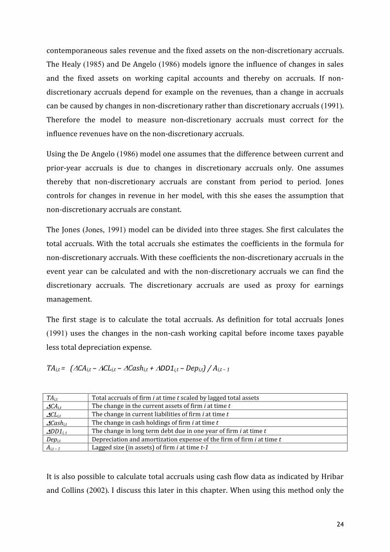
The  first  stage  is  to  calculate  the  total  accruals.  As  definition  for  total  accruals  Jones 

(1991)  uses  the  changes  in  the  non‐cash working  capital  before  income  taxes  payable 

less total depreciation expense.  

TAi,t =   ( CAi,t –  CLi,t –  Cashi,t +  DD1i,t – Depi,t) / Ai,t – 1 

 TAi,t   Total accruals of firm i at time t scaled by lagged total assets CAi,t   The change in the current assets of firm i at time t CLi,t   The change in current liabilities of firm i at time t Cashi,t   The change in cash holdings of firm i at time t DD1i, t  The change in long term debt due in one year of firm i at time t Depi,t   Depreciation and amortization expense of the firm of firm i at time t Ai,t – 1   Lagged size (in assets) of firm i at time t‐1   

It is also possible to calculate total accruals using cash flow data as indicated by Hribar 

and Collins (2002). I discuss this later in this chapter. When using this method only the 

25

first step of the Jones model changes. The calculated total accruals are used in the next 

two steps of the Jones (1991) model to find discretionary accruals. 

The  second  stage  is  to  estimate  the  coefficients  in  the  equation  for  non‐discretionary 

accruals using the total accruals calculated in stage one.  Jones (1991) uses a regression 

model  to  estimate  the  coefficients  in  the  formula  for  non‐discretionary  accruals.  The 

Jones (1991) model is an event model; it assumes that firms do not manage earnings in 

the years before the event. The time‐series of the firms earnings can be separated in an 

estimation period where discretionary accruals are zero and the event period (Ronen &

Yaari, 2008). 

To  estimate  these  coefficients  total  accruals  are  used  as  dependent  variable  in  the 

regression analysis. The coefficients of the formula can be estimated using a time series 

model or a cross‐sectional model. I will further explain the difference between these two 

and the advantages and disadvantages of both later in this chapter. In both versions the 

coefficients  are  estimated  on  an  estimation  sample,  this  can  be  the  years  prior  to  the 

event period (time‐series) or other companies in the industry (cross‐section).  

The first part of the second stage is to estimate the coefficients in the formula using total 

accruals as dependent variable.  

TAi,t =   1 × ( 1/ Ai,t‐1) +  2 × (∆REVi,t) +  3 × (PPEi,t) +ei,t  TAi,t  Total accruals scaled by lagged total assets of company i in year t Ai,t‐1  Lagged total assets of company i ∆REVi,t  The change in revenue scaled by lagged total assets of company i in year t PPEi,t  The gross value of property, plant, and equipment in year t for firm i ei,t  Residual of the model  

In  this  equation  the  change  in  revenues  and  gross  property  plant  and  equipment  are 

included  in  the model.  Jones  (1991)  ads  these variables  to  control  for  changes  in non‐

discretionary  accruals  caused  by  changing  conditions  in  the  environment  of  the 

company. The equation is estimated with an OLS‐regression. When using a time‐series 

approach coefficients are estimated on basis of a time‐series prior the year in which one 

wants to measure earnings management. For this estimation data is needed of the years 

preceding  the  event  year.  One  needs  approximately  10  years  prior  to  the  event  year. 

Though normally  the equation  is  estimated on  the  longest  time series of observations 

26

available prior to year t‐1 for each firm. Jones states that using the longest time series of 

observations  improves  estimation  efficiency  but  the  downside  of  a  long  estimation 

period  is  that  the  likelihood  of  structural  changes  in  the  period  increases.  Structural 

changes  in  the  company  can  contaminate  the model  because  the  accruals  before  and 

around the structural change are no good measure for the accruals in the event year.  

Jones  (1991)  uses  the  change  in  revenue  as  a  control  variable  because  total  accruals 

contain  changes  in  working  capital  accounts.  For  example  the  change  in  accounts 

receivable,  the  change  in  inventory  and  the  change  in  accounts  payable.  These  items 

depend to a certain degree on the changes in revenue. By adding the change in revenue 

as  an  independent  variable  Jones  (1991)  controls  for  this  effect,  assuming  that  the 

change  in  revenue  is  an  objective  measure  of  the  firms’  operations  before  earnings 

management takes place. This assumption might not be completely  justified;  therefore 

this  is  later changed  in  the modified version of  the  Jones model, discussed  in  the next 

part of this chapter.  

Gross property, plant and equipment is the other independent variable Jones (1991) uses 

in her regression model. Gross property plant and equipment is included as independent 

variable to control for the part of total accruals that is due to regular (non‐discretionary) 

depreciation expenses.  Jones  (1991) uses Gross property plant and equipment and not 

the change in gross property plant and equipment because the total annual depreciation 

expense is part the total accruals model. All variables in the formula are scaled by lagged 

assets, this is done to mitigate the effect of heteroscedasticity.  

The  third  stage  is  to  derive  the  discretionary  accruals.  As  total  accruals  contain 

discretionary  accruals  and  non‐discretionary  accruals  one  can  easily  derive  the 

discretionary accruals, as non‐discretionary accruals are known.  

DAi,t= TAi,t – NDAi,t   DAi,t  Discretionary accruals scaled by lagged total assets TAi,t  Total accruals scaled by lagged total assets NDAi,t   Non‐discretionary accruals scaled by lagged total assets 

3.5 Modified Jones model 1995 A  problem with  the  Jones  (1991)  model  is  that  the  sales  of  the  company  are  used  to 

control  for  the  firm’s  economic  circumstances.  Credit  sales  however  can be  subject  to 

earnings management themselves, because credit sales can be managed by moving them 

27

from period to period or by changing the bad debt policy.  Dechow et al. (1995) present a 

model  that  solves  this problem. They use  cash sales  instead of  total  sales;  they obtain 

cash sales by deducting the change in accounts receivable from the change in revenue.  

When  using  time‐series  version  of  the modified  Jones model  the  total  accruals  (stage 

one of the Jones model) are calculated with the normal Jones model and the coefficients 

are  estimated  with  the  normal  Jones  model  as  well  (stage  two  of  the  normal  Jones 

model). In the event period the non‐discretionary accruals are then calculated with the 

modified version of  the  Jones model. When using  the modified  Jones model  in a  cross 

sectional research design the modified Jones model is used for the estimation of normal 

accruals  and  for  calculating  non‐discretionary  accruals.  This  is  the  formula  of  the 

modified Jones model: 

NDAi,t =  0 +  1 × ( 1/ Ai,t‐1) +  2 × (∆REVi,t ‐ ∆AR i,t)+  3 × PPEi,t  NDAi,t  Non‐discretionary accruals scaled by lagged total assets of company i in year t Ai,t‐1  Lagged total assets of company i ∆REVi,t  The change in revenue scaled by lagged total assets of company i in year t  ∆ARi,t  The change in accounts receivable scaled by lagged total assets of company i in year t.  PPEi,t  The gross value of property, plant, and equipment scaled by lagged assets in year t for firm i.   

When  using  the  modified  version  of  the  Jones  model  one  assumes  that  changes  in 

revenue  les  changes  in  accounts  receivable  are  free  from  earnings  management.  One 

also  assumes  that  changes  in  accounts  receivable  are  abnormal,  because  changes  in 

credit‐sales are seen as discretionary.  

Although  the  Jones and  the modified  Jones models have  their  shortcomings  they have 

been  important  in this  field of research. They have been used frequently and different 

people have improved and extended the models. The next two sections discuss using the 

models in different ways: time series versus cross sectional and the use of balance sheet 

accruals  versus  cash  flow  accruals,  after  these  sections  I  discuss  improved  accrual 

models most of them based on the Jones model. 

3.6 Time‐series versus cross sectional Jones models There  are  two  possible  research  designs  in which  the  different  versions  of  the  Jones 

models can be used. The first one uses the Jones model in a time‐series design. The other 

option is to use the Jones model in a cross sectional research design. When using a time‐

series research design one uses the data of a company from the years prior to the year 

28

where one wants  to measure earnings management  to estimate  the coefficients  in  the 

formula  for  non‐discretionary  accruals.  The  period  in  which  one  wants  to  measure 

earnings  management  is  the  event  period.  The  years  before  that  are  called  the 

estimation  period.  In  a  cross‐sectional  research  design  one  estimates  the  normal 

accruals on a sample of companies from the same industry. In the cross‐sectional design 

data  from the same year but  from other companies  in the  industry  is used to estimate 

the normal accruals.  

3.6.1 Time‐Series designs with the Jones model When using  the  Jones model  in  a  time‐series version we distinguish  two periods. The 

event year,  that  is  the year  in which one wants  to measure earnings management and 

the estimation period, these are the years, preferably 10 or more, prior to the event year. 

The data  from  these  years  is  used  to  estimate  the  coefficients  of  the  formula  for non‐

discretionary  accruals.  If  one  uses  the  model  in  this  way  one  makes  the  implicit 

assumption  that  there  is no earnings management  in  the estimation period.  “Earnings 

management  in  the  estimation  period  contaminates  the  test  (Ronen & Yaari, 2008)”, 

because that level of earnings management will be seen as normal and will therefore be 

no  part  of  the  discretionary  accruals.  Another  implication  of  the  time‐series model  is 

that is requires a long series of observations. Therefore it is likely that a firm adapts its 

business‐and accruals policies in that time. Changing business and accrual policies will 

have an effect on the accruals; therefore the measurement will be influenced.  

Using a time series model may also create a selection bias, because firms have to survive 

at least 10 years to be able to carry out a time series research. The bias arises because 

such  firms  are  more  likely  to  be  bigger  more  mature  firms.  These  firms  have  other 

priorities  than  smaller  younger  firms.  For  example:  Established  firms  may  have  a 

carefully build reputation which they don’t want to risk by using earnings management 

(Ronen & Yaari, 2008).  

The most important argument in favor of using a time‐series model is that it uses data of 

the company where we want to test earnings management to estimate the coefficients in 

the formula for non‐discretionary accruals. The advantage of using data from the same 

company is that it is much more likely that the data is better comparable with the data of 

the  event  year  were  we  want  to  measure  earnings  management  because  this 

information  is  firm‐specific. Because a company stays, unless major changes,  the same 

29

company  from  year  to  year  we  can  predict  the  normal  or  expected  accruals  more 

accurately using this method. While using information from other companies will always 

have the problem that not two companies are the same.  

3.6.2 Cross‐sectional designs with the Jones model When used in a cross‐sectional design the non‐discretionary accruals are estimated on a 

sample of firms in the same industry, instead of data of the same firm from prior years. 

This  implies  that  the  coefficients  obtained  are  now  industry‐specific  instead  of  firm 

specific. 

With the coefficients estimated one is than able to obtain the non‐discretionary accruals 

of the company of which we want to measure earnings management. The sic codes are 

often used for grouping the firms per industry; to obtain a larger sample the two digit sic 

code is often used.  

A cross‐sectional research design has disadvantages as well. It is questionable whether 

the benchmark used: the other companies in the industry, is an appropriate benchmark. 

The cross‐sectional design assumes  that  there  is homogeneity within  the  industry;  for 

instance that companies have the same operating technology which gives the same level 

of normal accruals for a certain level of performance. It could be the fact that the other 

companies deviate too much from the company tested. Therefore those companies have 

different  normal  accruals.  This  contaminates  the  estimation  of  the  coefficients  in  the 

accrual  formula.  The  grouping  of  companies  per  industry  is  important;  hence  how 

industries are defined, because aggregating companies  that have  little  in common will 

negatively  affect  the  result  as  in  that  case  the  bench mark where  the  coefficients  are 

estimated on is not representative (Ronen & Yaari, 2008).  

Another possible problem with a cross‐sectional design is that the observations used for 

estimating  the  coefficients  may  include  managed  earnings.  If  other  companies  in  the 

industry manage earnings as well  this will be  the  fact, normal accruals  then  contain a 

part  of  the discretionary  accruals.  The  Jones model will  in  such  a  case only  recognize 

earnings management  if  the  earnings management  is  relatively  high  compared  to  the 

earnings management used in the industry. In times of economic prosperity companies 

may decide to smooth the earnings, therefore the “normal” accrual in this industry will 

30

be negative. Only if the accruals of the tested company are more negative than those in 

the industry earnings management is recognized.  

A weak point in the sample selection is that normally only industries with more than 8 

or 10 observations are used; therefore some industries are excluded from the test.  

Whether  to use  a  cross‐sectional  or  a  time‐series  design depends on  the  assumptions 

one  wants  to  make.  It  depends  on  which  assumptions  are  the  most  realistic  for  the 

particular research design. If a cross sectional sample contains a large number of firms 

that  are  similar  to  the  firm where  we want  to measure  earnings management  in  the 

sense that they are for example all mature firms and have a comparable operating cycle, 

the cross sectional approach will suit. If we want to measure earnings management in a 

relatively  new  company  there  will  be  no  data  for  the  time  series  approach,  than  the 

cross sectional method is the solution. Cross sectional designs sometimes considered as 

the better designs as  these models have greater power due to  lager samples  (Ronen &

Yaari, 2008). 

3.7 Difference between balance sheet accruals and cash flow accruals Earnings  consist of  a  cash component and an accrual  component. The  first  step of  the 

Jones  (1991)  model  is  to  calculate  the  total  accruals,  hence  the  accrual  component  of 

earnings.  There  are  two  main  approaches  to  determine  the  accrual  component  of 

earnings:  the  balance  sheet  approach  and  the  cash  flow  approach.  The  balance  sheet 

approach calculates accruals using  information  from the balance sheet. These accruals 

are  derived  from  the  change  in  non‐cash  working  capital.  The  other  approach  is  to 

calculate total accruals using cash flow information.  

Hribar and Collins (2002) show that when using time series models in combination with 

balance  sheet  information  problems  can  occur  around  non‐articulation  dates.  The 

balance  sheet  approach  is  an  indirect  approach  to  calculate  accruals, when  using  this 

approach  one  assumes  that  there  is  articulation  between  the  accrual  component  of 

revenues and expenses in the income statement and changes in balance sheet working 

capital  items. This assumption however does not hold  for non‐operating events. These 

are  for  instance:  mergers,  acquisitions,  reclassifications,  accounting  changes, 

divestitures and foreign currency translations (Hribar & Collins, 2002).  

The following formula is used to calculate balance sheet accruals: 

31

TAi,t = ( CAi,t –  CLi,t –  Cashi,t +  STDi,t – Depi,t) / Ai,t – 1 

 TAi,t   Total accruals of firm i at time t lagged by total assets CAi,t   The change in the current assets of firm i at time t CLi,t   The change in current liabilities of firm I at time t Cashi,t   The change in cash holdings of firm i at time t STDi,t   The change in long term debt in current liabilities of firm i at time t Depi,t   Depreciation and amortization expense of the firm of firm i at time t Ai,t – 1   Lagged size (in assets) of firm i at time t‐1   

Changes in working capital due to a non‐operating event are visible in the balance sheet 

but  do  not  flow  through  the  income  statement.  Therefore,  some  of  the  changes  in 

balance sheet working capital accounts relate to the non‐operating events. These could 

falsely be shown as accruals when using balance sheet approach (Hribar & Collins, 2002). 

In the case that mergers and acquisitions (from here on M&A) increase working‐capital 

accruals,  the normal accruals are estimated higher  than  they should. Which  leads  to a 

positive  bias  in  the  normal  accruals  and  thereby  to  a  negative  bias  in  discretionary 

accruals. Divestitures have the opposite effect on the accruals (Ronen & Yaari, 2008). 

Foreign  currency  translations  have  no  effect  on  the  earnings  reported  in  the  income 

statement  as  those  are  only  recognized  in  the  comprehensive  income  on  the  balance 

sheet.  The  bias  in  balance  sheet  accruals  caused  by  foreign  currency  translations 

depends on whether the main currency of the company strengthens or weakens.   

To mitigate the bias around the non‐articulation events as M&A and divestitures one can 

use a measure for total accruals that is based on cash flow data instead of balance sheet 

information.  Using  cash‐flow  accruals  solves  the  problem  around  non‐articulation 

events because  the changes  in  investment activities around non‐articulation events do 

not flow through the cash‐flow statement.  

The  total  accruals  are  calculated  as  the  difference  between  earnings  before 

extraordinary  items  and  discontinued  operations  –  operating  cash  flows  from 

continuing operations scaled by total assets.  

TAi,t = (EBXIi,t – CFOi,t)/ Ai,t‐1 

TAi,t   Total accruals of firm i at time t scaled by lagged total assets. EBXIi,t  Earnings before extraordinary items and discontinued operations 

32

CFOi,t  Operating cash flows from continuing operations Ai,t ‐1  Total assets  

Hribrar and Collins (2002) conclude that it is prudent for researchers to rely on accrual 

measures  taken  directly  from  the  cash  flow  statements,  because  these  do  not 

contaminate the test around non‐articulation events. A possible problem with cash flow 

accruals  in  certain  research  designs  can  be  that  cash  flow data  is  only  available  from 

1987 onwards.  

3.8 Improved versions of the Jones model  The  Jones  (1991)  and  the modified  Jones model attempt  to separate total accruals  into 

non‐discretionary  (normal)  and  discretionary  (abnormal)  accruals.  The  Jones  (1991) 

model  is  criticized  for  not  correctly  separating  the  accruals  in  non‐discretionary  and 

discretionary  accruals.  This  is  due  to  the  fact  that  the  model  for  non‐discretionary 

accruals in incomplete (Bernard & Skinner, 1996). It is very difficult or maybe impossible 

to  exactly  determine  the  normal  accruals,  but  since  the  Jones  (1991)  model  more 

advanced  models  have  been  designed  which  improve  the  estimation  of  the  non‐

discretionary accruals. In this part I discuss different models that are improved versions 

of  the  Jones  (1991) model.  They mitigate  some  of  the weak  points  of  the  Jones  (1991) 

model and therefore generate a more reliable measure of discretionary accruals than the 

Jones and modified Jones (1991) models.   

3.9 The forward‐looking model 2003 Dechow,  Richardson  and  Tuna  (2003)  improve  the  cross‐sectional  version  of  the 

modified Jones model. They present three improvements on the Jones (1991) model that 

enhance the reliability of the model. De model designed by Dechow et al. (2003) is called 

the forward‐looking model.  

The first improvement they introduce is that they make an adjustment for the expected 

increase  in  credit  sales.  The  modified  Jones  (1991)  model  treats  all  credit  sales  as 

discretionary;  this  might  not  be  entirely  just.  It  causes  a  correlation  between 

discretionary  accruals  and  sales  growth.  Dechow  et  al.  (2003)  do  a  regression  to 

estimate a sales coefficient that the expected change in accounts receivable for a certain 

change  in  sales. The model  treats  this  expected change  in accounts  receivable as non‐

33

discretionary. Where  the  modified  Jones  (1991)  model  would  treat  al  credit  sales  as 

discretionary. 

Dechow et al. (2003) use the following regression to estimate the sales coefficient: 

∆AR =   + K × ∆sales + e  

∆ AR   The change in accounts receivable K  Coefficient for the expected change in accounts receivables for a given change in sales ∆ sales   The change in sales  

K  measures  the  sensitivity  of  the  change  in  non‐discretionary  accounts  receivable  to 

sales. If K is 1, 100% of the change in accounts receivable is non‐discretionary if K is 0 

100% of the change in accounts receivable is discretionary. Adding K to the Jones (1991) 

model  adds  non‐discretionary  accounts  receivable  in  sales  to  the  cash  sales  (both 

discretionary).  The  slope  coefficient  is  added  to  the  cross‐sectional  modified  Jones 

model (Dechow, Sloan, & Sweeney, 1995). 

The second improvement Dechow et al. (2003) apply in their model is that they control 

for so called ‘reversals’. Reversals are the consequences of accounting decisions made in 

the previous period. Accruals by definition reverse trough time, they are less persistent 

than cash flows. To control for this effect the lagged value of total accruals is added to 

the model.  

Accruals are used to turn the continuous cash flow of the company in an annual income 

statement. Therefore accruals are per definition designed to smooth the reporting of the 

financial  performance  of  the  company.  For  example  a  firm  that  grows  and  therefore 

anticipates  a  future  sales  grow will  increase  its  inventory.  In  this  case  the  increase  in 

inventory is not due to earnings management. But the Jones model would classify this as 

discretionary  accruals.  To  control  for  this  mistake  Dechow  et  al.  (2003)  include  a 

measure of future sales growth.  

The change in sales from the current year to the subsequent year scaled by current sales 

is used as measure for the future sales growth. Therefore this item is only available if the 

financial statement of the year following the event year is available. If this is not the case 

the lagged value of this measure can be used, as Dechow et al. (2003) do.  

GR_Salest =  (salest+1 – salest) / salest GR_Sales  Measure for the future sales growth sales i,t+1   Sales of the year after the event year of company t sales i,t  Sales in the event year of company t  

34

With these modifications Dechow et al. (2003) compose the following model:  

TAi,t=  1 +  2((1+K) ∆salesi,t ‐ ∆ARi,t) +  3PPEt +  4 (TAi,t,‐1/ Ai,t‐2) +  5 GR_salesi,t  

   TA  Total accruals in the current year of firm i, scaled by year t‐1 total assets. ∆sales     Change in sales, scaled by year t‐1 property plant and equipment ∆AR  The change in accounts receivable, scaled by year t‐1 total assets.   K  The slope coefficient from a regression of ∆AR on ∆sales PPE  Gross property plant and equipment TAi,t,‐1/ Ai,t‐2  Total accruals from the year before the current scaled by total assets of two years ago for 

firm i. GR_sales  The change in sales for firm i, from year t to t+1, scaled by year t sales.  

 

3.10 Cash flow Jones model 2002 Dechow and Dichev (2002) focus on the quality of earnings and accruals. They state that 

the quality of measured accruals depends on the mistake in predicting cash flows. This is 

due to the  fact  that accruals separate the timing of cash  flows and their recognition  in 

the  financial  statements.  If  an  expense  is  booked  before  the  cash  flow  takes  place  an 

accrual is created. This accrual is the predicted future cash flow.  

Until the Dechow and Dichev (2002) thesis most models did not control for cash flow in 

their  accruals model.  This  had  to  do with  the  possible  simultaneity  problem.  As  cash 

flows are by definition the difference between earnings before extraordinary items and 

accruals. This causes the simultaneity problem especially if the cash flow method is used 

to calculate the total accruals (Ronen & Yaari, 2008).  

They define earnings as cash flows and accruals: 

Earnings= cash flow + accruals 

From an  accounting point  of  view  there  are  two  important  events  for  each  cash  flow. 

The first is the receipt or payment of the amount. The second is the recognition of this 

amount as profit or loss.  

Cash flows for a certain period “t” can be divided into three groups: 

CFt‐1t= cash receipts or payments of amounts accrued at t‐1 

CF t,t = current cash flows 

CF t+1,t= cash flows postponed to the next period 

35

As you can see there is a sub script and a super script behind the variable, the sub script 

is the period in which the amounted is booked as earning or expense. The super script 

refers to the period in which the amount is received or paid.  

The total cash flow for a period “t” consists of: 

CFt = CFt‐1t + CFtt + CF t+1t 

Dechow and Dichev  (2002)  assume that working capital accruals are solved within  the 

next period. For example  if  in period  “t” a  sale on  credit  is done and  the earnings are 

realized,  than  in  the  next  period  the  payment  is  done  and  the  accrual  is  solved. 

Therefore the change in working capital in a certain year is influenced by the cash flow 

of the prior year, the current cash flow and the cash flow of the next year.  

In case the cash flow follows after the revenue or expense is recognized managers have 

to estimate what cash flow will follow in the future. The real cash flow might defer from 

the  cash  flow  that was  anticipated.  If  the  realized  cash  flows  defer  from  the  accruals 

estimations than the opening accruals (the accruals made when the future cash flow was 

estimated)  contain an error  that  is  corrected by  the  closing accrual  (the accrual made 

when the final cash flow takes place). 

Dechow and Dichev (2002) conclude about accruals: 

‐ That accruals are temporary adjustments that delay or anticipate the recognition 

of realized cash flows plus an estimation error term. 

‐ Accruals  are  negatively  related  to  current  cash  flows  and  positively  related  to 

past and future cash flows.  

‐ The error term measures to what extent  the cash  flow realizations matches the 

accruals; it can be used of a measure of accrual and earnings quality. 

Dechow and Dichev (2002) express accruals with the following equation:  

TAt= CFt‐1t – (CFtt+1 + CFtt‐1) + CFt+1t + εt+1t – εtt+1 

TAt  Current total accruals recognized in period t CFt s  Cash from operations realized in period t and recognized in period s Εt s  Error term, for accruals recognized in period s and cash flows realized in period t  

36

The  error  term  is  this  regression  represents  accruals  that  are  not  related  to  the 

realizations of predicted cash flows. This error term is used as measure for the quality of 

earnings and accruals. 

The following formula is made by, Dechow and Dichev (2002) to find a practical measure 

for working capital accruals. They use the equation in a time series test.  

∆WCt=  0 +  1 CFOt‐1 +  2 CFOt +  3 CFOt+1+  t ∆ WC   The change in working capital3 CFO  Cash flow from operations t  An error term, used to measure the quality of earnings  

The  first of  these  formulas  (the  theoretical) uses  components of  the past, present and 

future cash flows. Because it is not possible to identify these components of cash flows, 

the second (more practical) formula is made that uses cash flow from operations. Since 

cash  flow  from  operations  includes  cash  flows  realized  in  a  certain  period  that  are 

recognized in different periods this leads to an estimation error4. The standard deviation 

of the residual is used as measure for earnings quality. 

This error term does not only contain earnings management but can also reflect  firms 

that  report  honestly but  face uncertain  economic  environments  and  are  therefore not 

able  to  properly  predict  future  cash  flows  or  firms  whose  managers  are  not  good  at 

estimating future cash flows (McNichols, 2002).  

McNichols  (2002)  discusses  the  Dechow  and  Dichev  (2002)  thesis  in  her  work.  She 

recognizes  a  couple  drawbacks  of  the model.  Dechow  and  Dichev  (2002)  assume  that 

accruals  are  solved within  the next period;  therefore  the model  only works  for  short‐

term  accruals.  That means  that  their measure  is  not  suited  to  use  for  companies  that 

work with a production cycle that takes more time than one accounting period.  

A  second drawback of  the model  is  that  the  two estimation  errors  are  assumed  to be 

independent of each other and of the cash flow realizations. However estimation errors 

in the case of discretionary accruals are likely to depend on each other and on the cash 

3 The change in working capital, measured as the sum of the change in accounts receivable + the change in inventory minus the change in accounts payable minus the change in tax payable plus the change in other net assets net of liabilities. All these variables are scaled by average total assets (Ronen and Yaari 2008). 4 See Dechow and Dichev (2002), the coefficients are likely to be biased towards 0 and the R2 is lower.

37

flow  realizations.  Therefore  the  model  might  not  apply  in  the  context  where 

management uses earnings management (McNichols, 2002).  

McNichols  (2002)  links  the  work  of  Dechow  and  Dichev  (2002)  with  the  literature  on 

discretionary accruals and especially the Jones model. Where the Jones model focuses on 

separating total accruals into discretionary‐ and non‐discretionary accruals the Dechow 

and Dichev (2002) thesis focuses on total accruals. A weakness of the Jones model is that 

discretionary  accruals  estimated  with  the  Jones  model  are  not  pure  discretionary 

accruals,  hence  they  also  contain  in  part  accruals  that  are  due  to  other  things  than 

earnings  management.  McNichols  (2002)  points  out  two  examples  of  factors  that 

contaminate  the  discretionary  accruals  in  the  Jones model.  The  first  is  that  the  Jones 

model assumes that accruals react to the current change in sales, but does not take into 

account  future  and  lagged  changes  in  sales.  The  second  factor  that  McNichols  (2002) 

points out in her study is that the Jones model ignores the expected future sales growth. 

McNichols  (2002)  finds,  as  Dechow  and  Dichev  (2002)  do  that:  prior,  current,  and 

subsequent years cash flow from operations is correlated with the Jones model.  

Ye  (2007) points at another weakness  in the model by Dechow and Dichev  (2002). The 

model shows the relation between accruals and cash flows. A problem with the measure 

proposed  is  that  it excludes earnings management committed by shifting  income from 

period to period, as that shifting satisfies the measure proposed in the thesis. However 

this can be an important earnings management tool.  

3.11 Larcker and Richardson 2004 Larcker and Richardson (2004) improve the measurement on non‐discretionary accruals 

by adding the book‐to‐market ratio and current operating cash flows to the model. 

The book‐to‐market ratio is included to control for the expected growth in a company’s 

operations. This variable  is added because growing firms show high  levels of accruals. 

Growing  companies  are  expected  to  invest  more  in  inventory  and  other  assets. 

Therefore  an  increase  in  inventory  for  a  growing  company  is  probably  not  due  to 

opportunistic behavior. To control for wrongly qualifying these accruals as discretionary 

the book‐to‐market ratio is added to the model. The book‐to‐market ratio is calculated 

as the book value of common equity divided by the market value of common equity.  

38

Dechow et al.  (1995)  conclude that  firms with extreme performance are more  likely to 

have  miss‐specified  discretionary  accruals.  To  control  for  this  miss  specification  the 

current  operating  cash  flow  is  used  as  extra  independent  variable  in  the  model.  The 

model Larcker and Richardson (2004) use is the following: 

TAi,t =  0 +  1 ×  ( ∆REVi,t− ∆ARi,t ) +  2  × PPEi,t +  3  × BMi,t +  4 ×  CFOi,t + εi,t  

TAi,t   Total accruals of company i at time t scaled by average total assets ∆REVi,  The change in revenue of company i at time t scaled by average total assets ∆ARi,t   The change in accounts receivable of company i at time t scaled by average total assets PPEi,t   The gross value of property, plant and equipment of company i at time t scaled by 

average total assets BMi,t   The book to market ratio company i at time t scaled by average total assets CFOi,t   The current operating cash flow company i at time t scaled by average total assets ε  Residual  

Larcker and Richardson (2004) use the cash flow approach to calculate the total accruals. 

They state that it is better to use the extra control variable in the accrual formula than in 

the final regression analysis were accruals are linked with another measure, depending 

on the research. This is better because adding he control variables in the cross‐sectional 

accrual model makes it possible to identify industry year specific coefficients for these 

variables.  

3.12 Performance matching model 2005 Kothari, Leone and Wasley (2005) present another much used improvement on the Jones 

model. Their model controls for performance related accruals. The accruals this model 

controls for are performance related accruals that are classified as discretionary under 

the modified Jones Model. These accruals are however not due to earnings management 

but are a result of the performance of the company.  As in this master’s thesis I want to 

measure earnings management due to equity incentives it is extra important to control 

for  firm  performance,  because  of  the  correlation  between  firm  performance  and 

compensation (Ronen & Yaari, 2008).  

Accruals are correlated by performance, in other words there is a relation between the 

firms current and past performance and the accruals. Kothari et al. (2005) describe this 

relation  in  their  thesis;  if  forecasted  sales  changes  are  not  zero  or  when  other 

parameters affecting accruals change  than  the  forecasted accruals are non‐zero. When 

sales  changes  are  predictable,  earnings  changes will  also  be  predictable  and  expected 

39

accruals will  therefore  be  non‐zero.  The  predictability  in  future  performance  leads  to 

predictable  future  accruals.  The  accruals  model  needs  to  filter  these  performance‐

related  component  out  of  the  discretionary  accruals.  Otherwise  this  leads  to  false 

discretionary accruals.  

Kothari et al. (2005) present two ways to do this. The first one is adding return on assets 

to  the  modified  version  of  the  Jones  model  to  control  for  the  performance  of  the 

company.  Thereby  improving  the  linear  accrual  model.    The  second  method  is  to 

calculate  discretionary  accruals  by  comparing  the  discretionary  accruals  two 

comparable companies, where one of  the  two  is expected  to manage earnings and  the 

other not. In this method Kothari et al. (2005) abandon the path of the linear regression 

model to calculate discretionary accruals.  

The essence of  the second method  is  that  there are  two groups of  firms,  two samples: 

The  measurement  sample,  this  is  the  sample  were  one  wants  to  measure  earnings 

management  and  the  control  sample  in  which  no  earnings  management  takes  place. 

Firms  from  the measurement  sample have  to be matched with  firms  from  the  control 

sample  that  have  a  similar  return  on  assets.  This  is  the  control  for  performance,  the 

firms are similar and have similar performance therefore similar accruals are expected. 

The  Jones model  is  used  to  calculate discretionary  accruals  for both  sets  of  firms,  the 

accruals in the control sample al seen as the normal accruals. The abnormal accruals are 

than calculated as  the difference between  the discretionary accruals of  the  firm  in  the 

measurement sample and the discretionary accruals of the firm in the control sample by 

deducting  the  discretionary  accruals  of  the  firm  in  the  control  sample  from  the 

discretionary accruals of the matched firm in the measurement sample. To successfully 

do  this  it  is  important  that  firms  are matched with  a  comparable  firm.  Kothari  et  al. 

(2005) therefore match firms on industry by using the two digit sic code and on return 

on assets. The goal is that the matched firms are almost identical except the fact that one 

is  in  the  measurement  group  and  the  other  in  the  control  sample.  An  essential 

assumption  in  this  model  is  that  the  firms  in  the  control  sample  are  not  involved  in 

earnings management.  

A second assumption that Kothari et al. (2005) make is that firms (that are similar) with 

the  same  performance  have  the  same  discretionary  accruals.  The  firms  in  the 

40

measurement sample are in that sample because earnings management is expected for 

these  firms  for example because  these  firms have gone  through a certain event where 

earnings management is expected, or they have certain characteristics that the firms in 

the  control  sample  do  not  have.  The  event  or  the  characteristics  are  the  reason  for 

expected  earnings  management.  For  instance  the  measurement  firms  use  equity 

incentives and the control firms do not.  

For this method it  is  important to be able to match the firm with a control firm that  is 

comparable. One assumes that there is no earnings management in the control firm. For 

this way of measuring accruals firms one needs a reliable control sample of which one 

expects no earnings management. Therefore one needs a sample of firms that are similar 

but have not gone through that certain event or do not have those characteristics. 

In their  linear approach Kothari et al. (2005)  improve the modified Jones model  in two 

ways; they add an intercept to the model and control for the company’s performance by 

adding return on assets to the model. The first term in the modified Jones model is the 

inverse  of  lagged  assets,  the  inverse  of  lagged  assets  is  used  in  the model  to mitigate 

heteroscedasticity.  Despite  this,  heteroscedasticity was  still  in  a  problem  in  the  Jones 

(1991)  model,  Kothari  et  al.  (2005)  ad  an  extra  intercept  to  further  reduce 

heteroscedasticity.   

In the Linear model return on assets is added as independent variable to control for the 

effect of prior performance on the discretionary accruals. Kothari et al. (2005) choose to 

use  return  on  assets  as  control  variable  for  prior  firm  performance  because:  “by 

definition earnings deflated by assets equals return on assets, which  in  turn measures 

performance.”  The  other  argument  to  use  return  on  assets  Kothari  et  al.  (2005)  bring 

forward is that prior research proves that return on assets is better specified and more 

powerful than other control variables for firm performance.  

An  important  question  is  whether  controlling  for  performance  does  not  lead  to  over 

controlling.  Controlling  comes  with  the  risk  that  we  remove  in  part,  discretionary 

accruals that result from earnings management. This could be the case because the firms 

in  the  industry where  the  cross‐sectional model  is  estimated on might have  the  same 

incentives to manage earnings when compared to the treatment firms. This is a possible 

weakness in the model. 

41

The Kothari et al. (2005) linear model:  

NDAi,t=  0 +  1 (1/Ai,t ‐1) +  2 ( REVi,t ‐  ARi,t) +  3 PPEi,t +  4ROAi,t‐1 

NDA  Non‐discretionary accruals scaled by lagged total assets 0   A constant, the intercept of the regression 1/Ai,t ‐1  1 divided by lagged total assets REV  The change in revenue scaled by lagged assets AR  The change in accounts receivable scaled by lagged assets PPE  Gross property plant and equipment scaled by lagged assets ROAi,t‐1  Lagged rate of return on assets   

3.13 The Business Model 2007 Ye  (2007)  introduces  a model  that  combines many  of  the  improvements made  in  the 

models  discussed  in  this  chapter.  Ye  (2007)  takes  together  the  improvements  of  the 

different  improved variants of  the  Jones model  to make a new model.  Besides  that he 

provides  important  insight as he shows that even  limited tweaking of  the  Jones model 

enhances  the power of  the model. When  improving  the  Jones  (1991) model numerous 

possibilities arise, Ye (2007) states that it is important to stop adding extra variables at a 

certain point.  

Ye  (2007)  also  finds a  solution  that mitigates a drawback of  cross‐sectional models,  in 

that cross‐sectional models do not take into account firm‐specific parameters. Ye (2007) 

ads three additional firm‐specific variables to mitigate this problem. 

In his thesis Ye (2007) shows how basic firm specific characteristics influence accruals. 

The  measures  he  discusses  are:  “the  level  of  beginning  abnormal  working  capital, 

working capital intensity and the useful life of a firm’s long term assets”. Ye (2007) states 

that  these  factors  are not  the  same within a  industry  and  also  change over  time  for  a 

company. 

The  first  measure  Ye  (2007)  ads  tries  to  mitigate  the  weakness  caused  by  reversing 

accruals. Ye (2007) uses the reversion of abnormal noncash working capital as his first 

measure. He states that in other models people have added lagged accruals to the Jones 

model  to  control  for  reversing  accruals,  an  example  of  such  a  model  is  the  forward 

looking  model  discussed  in  this  chapter.  This  however  does  not  improve  the  Jones 

model  according  to  Ye  (2007),  because  when  high  lagged  accruals  occur,  they  either 

compensate  for an abnormally  low working  capital  in  the previous year, or  they  raise 

42

the working capital to an abnormal level. The accruals are only in the second case likely 

to reverse. Therefore the accrual reversal should be based on the abnormal balance of 

working capital instead of lagged accruals. Ye (2007) uses the  lagged abnormal balance 

of  working  capital.  The  abnormal  balance  of  working  capital  is  the  amount  of  which 

contemporaneous working capital defers form normal working capital. Normal working 

capital  is  estimated  with  the  historical  values  of  non‐cash  working  capital.    The 

abnormal balance  can be  caused by  a  fluctuation  in business  activities  or by  earnings 

management during the previous period. An abnormal balance is expected to vanish in 

one operating cycle.  

The measure for the lagged balance of the abnormal non‐cash working capital is: 

ANCWCi,t‐1 = NCWCi,t‐1 – NNCWCit 

ANCWC  Abnormal non‐cash working capital NCWC  Non‐cash working capital NNCWC  Normal non‐cash working capital  

The second measure Ye (2007)  introduces is non‐cash working capital intensity. This is 

measured as the ratio of noncash working capital to sales or assets. Ye (2007) states that 

different firms have a different working capital intensity. The working capital intensity 

depends  on  the  nature  of  the  business  and  the  policy  of  the  firm.  These  aspects  can 

change over time and can be different for firms in the same industry. Ye (2007) gives as 

example that: “a one dollar increase in revenue leads to a higher increase in receivables 

for  a  firm  that  mostly  makes  credit  sales  than  for  a  firm  that  makes  cash  sales”. 

Therefore the effect of a change in revenue on accruals depends not just on the amount 

of  revenue  change,  but  also  on  its  working  capital  intensity.  The  second measure  Ye 

(2007)  introduces  mitigates  the  error  due  to  differences  in  working  capital  intensity 

among firms and for the change over time within one company.  The effect of an increase 

in the firm sales on current accruals is proportional to: lagged non‐cash working capital 

multiplied by the change in revenue, therefore this  is the second measure proposed by 

Ye (2007). This measure uses an up‐to‐date indicator for non‐cash working capital of a 

company. It therefore covers both to time series as the cross‐sectional difference in non‐

cash working capital between companies.  

Second measure: 

43

NCWCi,t ‐1 × ∆ REVi,t  

The third measure Ye (2007) uses are non‐current accruals. As the depreciation expense 

of a company depends on more than only the amount of assets. Ye (2007) states that the 

depreciation expense also depends on the average depreciation rate. A depreciation rate 

can be different between different companies in the industry but can also change within 

a firm. The depreciation rate changes depending on the stage of the company in the life 

cycle, changes in the life of assets, deprecation methods and the way the asset portfolio 

is made  up.  The  Jones  (1991)  model  assumes  the  deprecation  rate  is  constant,  this  is 

however not realistic. To reckon this, the lagged depreciation rate of a firm is added to 

estimate  the  current  depreciation  rate.  Ye  (2007)  defines  the  depreciation  rate  as 

follows: 

DEPRATi,t = DEPi,t / PPEi,t 

DEPRAT  Depreciation rate DEP  Depreciation expense PPE  Gross property plant and equipment  

Ye  (2007)  discusses  the  problem  of  unusual  observations.  Unusual  observations  may 

cause  problems  when  using  accrual  models,  even  when  using  large  datasets.  The 

problem becomes more severe when using firm or industry specific estimations because 

the sample size reduces in those cases.  

To mitigate this problem Ye (2007) proposes to winsorize the dependent variable on the 

first  and  the  99th  percentile.  The  independent  variables  are  truncated  at  the  first  and 

99th percentage.  

Kothari et al. (2005) point at the possibility of a nonlinear relation between accruals and 

performance variables  as ROA. As  solution  to  this problem  they propose performance 

matching, as discussed in this chapter. Ye (2007) states that this method is only effective 

if  there  is  only  nonlinearity  in  one  variable.  As  there might  be  non‐linearity  in more 

variables the matching method is not possible. Ye (2007) states that an effective method 

to  deal  with  the  nonlinearity  is  to  winsorize  the  independent  variable  further.  “For 

example winsorizing return on assets to a range of a normal return on assets ‐0.1 to 0.3 

reduces the nonlinearity in return on assets” (Ye, 2007). 

44

Ye (2007) combines his new variables with the linear version of the Kothari et al. model, 

which itself is a further developed Jones model. This is the model Ye (2007) designed: 

TAi,t =βo + β1 /Ai,t −1 + β2 ∆REVi,t + β3 PPEi,t + β4 ROAi,t−1 + β5 NCWCi,t −1 + β6 NNCWC,t + β7 

NCWCi,t−1 × ∆REVi,t + β8 DEPRAT,t −1 + β9 DEPRAT,t−1 × PPE i,t .  

TA  Total accruals ∆REV  The change in revenue PPE  Gross property plant and equipment ROA  Return on assets NCWC  Non‐cash working capital NNCWC  Normal non‐cash working capital DEPRAT  Depreciation rate (the depreciation divided by gross property plant and equipment) A  Total assets i  Subscript indicates the company t  Subscript indicates the year  

3.14 Recent literature on accrual models In addition to the accrual models discussed in this chapter I would like to point out two 

recent articles that discuss accrual models. The first is a model by Dechow, Hutton, Kim 

and Sloan  (2012),  their model  takes  into  account  that  accruals managed  in one period 

will  reverse  in  a  later  period.  Including  this  characteristic  of  accruals  “improves  the 

power and the specification of the tests for earnings management” (Dechow et al., 2012). 

In  order  to  include  the  reversal  of  accruals  in  the  tests  for  earnings  management 

researchers  have  to  be  able  to  identify  a  period  where  accruals  are  expected  to  be 

managed and the periods in which these accruals are predicted to reverse.  

The second is the article by Gerakos (2012). This article discusses the new accrual model 

introduced  by Dechow  et  al.  (2012).  Gerakos  (2012)  analyses  the model  introduced  by 

Dechow et al. (2012). Gerakos (2012) states that Dechow et al. (2012) make an important 

improvement  to  the  way  discretionary  accruals  are  measured,  their  most  important 

improvement  is  that  they  introduce  the  dynamics  of  accruals  to  the  discretionary 

accrual measures. These dynamics are the reversing of  the accruals  that Dechow et al.

(2012) use in their model. Besides introducing the reversal of accruals to the model they 

also identify a number of fundamental questions that are of interest for future research.  

 

45

3.15 Chapter 3 summary In  this  chapter  I  discussed  a  number  of  accrual models  that  can  be  used  to measure 

earnings management. Most of the more advanced models are based on the Jones model 

introduced  in  1991.  The  Jones  (1991) model  adds  to  the  research  as  it  finds  a way  to 

separate  the  total  accruals  in  discretionary‐  and  non‐discretionary  accruals.  In  the 

newer models, based in the Jones (1991) model, the way non‐discretionary accruals are 

estimated  is  more  refined.  This  leads  to  a  better  measure  of  discretionary  and  non‐

discretionary accruals.  

The  improvement  Jones  (1991) makes,  is  that  she  takes  into  account  the  effect  of  the 

contemporaneous sales revenue and the fixed assets on the non‐discretionary accruals. 

In  1995  the  modified  Jones  model  was  introduced  by  Dechow  et  al.  (1995),  in  the 

modified  Jones  model  cash  sales  are  used  as  control  variable  instead  of  total  sales. 

Because credit sales can be managed these are excluded from the model. The hindsight 

of  this  adoption  is  that  the  modified  Jones  model  assumes  that  all  credit  sales  are 

discretionary.  

The  Jones model  and  the models  based  on  the  Jones models  can  be  used  in  a  cross‐

sectional  and  in  a  times  series  test. Both have  their  strong and weak  sides,  the  cross‐

sectional model is however often described as the better of the two as it creates greater 

power  due  to  larger  possible  sample  sizes.    In  a  time  series model  one  assumes  that 

there is no earnings management in the estimation period, however this assumption is 

not always realistic. Another possible problem in a time series model is that there can be 

structural  changes  in  the  estimation  period,  these  contaminate  the  test.  Time  series 

models require a long series of observations, the model can only be used for companies 

that have  such a  time series  available  and  this may  lead  to  a  selection bias. The main 

advantage  of  a  time  series  analysis  is  that  company  specific  data  is  used.  A  cross‐

sectional  model  assumes  that  there  is  homogeneity  within  the  industry;  because  the 

accruals  are  estimated  on  a  sample  of  firms  in  the  same  industry  similarity  is  very 

important. A possible problem in the cross‐section can be that companies in the group 

where the coefficients are estimated on also commit earnings management.  

There are two ways to calculate accruals: one can use balance sheet information or cash 

flow information. Hribrar and Collis (2002) find that using cash flow information leads to 

better results around non‐articulation events. A reason not to use cash flow information 

46

can be  that  this data  is only available  from 1987 onwards, which can be a problem  in 

certain research designs.  

In  this  chapter  I  discussed  the  forward‐looking  model  (Dechow, Richardson, & Tuna,

2003), the cash flow model (Dechow & Dichev, 2002), the Larcker and Richardson model 

(2004), the Kothari et al. (2005) model and Ye’s syntheses model (2007).   

The  forward  looking  model  (2003)  is  an  improvement  on  the  Jones  (1991)  model,  it 

controls  for  the  future  sales  growth  and  it  refines  the  adoption made  in  the modified 

Jones model, by not excluding all credit sales but only the unexpected credit sales from 

the model.  

The cash flow model is not based on the Jones (1991) model, it uses total accruals, but it 

does  show  that  there  is  a  relation  between  accruals  and  the  preceding,  current  and 

subsequent cash flows. 

Larcker  and Richardson  (2004)  improve  the modified  Jones model  in  that  they  ad  the 

book to market ratio to control the effects of firm growth. They also ad cash flow from 

operations to control for firms with extreme performance.  

Kothari  et  al.  (2005)  provide  two  ideas  to  improve  the  Jones  model;  one  is  an 

improvement on the linear model where the return on assets is used to control for the 

performance of  a  firm  and an  extra  intercept  is  added  to mitigate heterostcedasticity. 

The other method abandons the linear path and measures discretionary accruals as the 

difference  between  the  accruals  of  two  similar  firms.  One  of  those  is  expected  to  use 

earnings management and the other is not.  

Ye  (2007)  introduces  a model  that  combines much  of  the  improvements  on  the  Jones 

model.  He  uses  the  linear model made  by  Kothari  et  al.  (2005)  as  basis. With  that  he 

introduces an alternative way to cope with the non‐linearity problem and he ads three 

firm specific variables. These variables reduce the weakness, caused the fact that cross‐

sectional models do not use firm specific information to estimate accruals.  

 

47

Chapter 4 estimating the equity incentives Different  measures  have  been  used  to  examine  the  relation  between  earnings 

management and incentives caused by remuneration. The proxy’s for equity incentives 

defer per research design and the availability of information.  

4.1 boundaries of bonus schemes As proxy for equity incentives the boundaries of bonus schemes have been used by for 

example Healy  (1985)  and Holtausen  et  al.  (1995).  They  expect  that managers manage 

earnings around the upper and lower bounds of bonus schemes to maximize their bonus 

over  the  years.  For  example  if  earnings  exceed  the upper bound of  the bonus  scheme 

managers are expected to manage earnings down in the current period to be able to use 

these  earnings  in  the  next  period  to  reach  the  bonus  target.  Healy  (1985)  compares 

accruals with estimated boundaries of bonus plans. He estimates  the upper and  lower 

boundary  of  bonus  plans  and  examines  the  accruals  around  these  boundaries.  Healy 

(1985)  assigns  observations  to  different  categories;  earnings  can  be  under  the  bonus 

range, in the bonus range or above the bonus range. He uses the estimated boundaries of 

bonus schemes to assign observations to the different categories. Because the estimated 

boundaries  of  bonus  schemes  are  used, mistakes  are made,  this makes  the model  les 

reliable.   Holthausen et al. (1995) use a similar design, the difference is that they use the 

real  upper  and  lower  bounds  of  bonus  plans  to  examine  accruals.  Holthausen  et  al. 

(1995) are able to do this as he uses inside information from human resource‐consulting 

firms. Healy’s method is weak because the boundaries of the bonus plans are estimated, 

as no data is available on the real boundaries of the bonus plans. This method does not 

lead to reliable results unlike the real boundaries of bonus plans can be used, therefore 

this data needs to be available.  

4.2 Maximizing earnings in Japan Shuto  (2007)  examines  the  relation  between  earnings  management  and  maximizing 

management  earnings  in  Japan.  Management  remuneration  in  Japan  is  different  from 

that in the United States. In Japan it is not common to use earnings based compensation 

for management, according to Japanese accounting rules companies are not required to 

disclose  information  on  executive  compensation.  This  makes  it  more  challenging  to 

measure  executive  compensation.  Otomasa  (2000)  explains  that  in  Japan  variable 

remuneration is different from the bonuses and stock remuneration we know in Europe 

48

in  the  United  States.  In  Japan  no  bonuses  are  awarded  but  executives  are  penalized 

when  the  firm  performance  worsens.  The  only  information  disclosed  considering 

remuneration  in  Japan  is  the  total  cash  compensation  for  the  complete  board.  This  is 

used as proxy  for executive compensation;  this  total compensation  is compared  to  the 

discretionary accruals calculated with the Jones model. In other words Shuto (2007) uses 

the total remuneration to management as proxy for incentives to manage earnings. 

Shuto  (2007)  finds  that  when  discretionary  accruals  increase  the  executive 

compensation increases as well and that in years with low payment earnings decreasing 

accruals and extraordinarily items can be found.  

4.3 Proxy for equity incentives The measures discussed  in  the  last  two sections  focused on bonus plan based or  total 

earnings incentives. This master’s thesis focuses on stock‐based incentives. Bergstresser 

and  Philippon  (2006)  introduce  a  measure  for  the  power  of  equity  incentives.  They 

measure  this as  the:  “dollar change  in  the value of a CEO’s stock and options holdings 

that  would  come  from  a  one  percentage  point  increase  in  the  company  stock  price”. 

They call this measure ONEPCT, and compute it with data from the “compustat executive 

compensation” database.  

ONEPCT i,t = 0.01 × PRICE i,t × (SHARES i,t + OPTIONS i,t) 

ONEPCT  The dollar change in the value of a CEO’s stock and options holdings that would come from a one‐percentage point increase in the company stock price. 

PRICE  The company share price SHARES  The number of shares held by the CEO OPTIONS  The number of options held by the CEO  

Bergstresser and Philippon (2006) use this measure to calculate their measure for equity 

incentives.  They  state  that:  “this  is  a measure  of  incentives  normalized  in  a way  that 

captures the share of a hypothetical CEO’s value in the equity of his or her company”. 

INCENTIVE RATIO i,t = ONEPCT i,t / ( ONEPCT i,t + SALARY i,t + BONUS i,t) 

INCENTIVE RATIO  The share of a CEO’s total compensation that would come from a one‐percentage point increase in the value of the equity of his or her company. 

ONEPCT  The dollar change in the value of a CEO’s stock and options holdings that would come from a one‐percentage point increase in the company stock price. 

SALARY  The cash salary awarded to the CEO BONUS   The cash bonus awarded to the CEO  

49

This measure implicitly assumes that if the share price changes the change of the value 

of the options is the same as the change in value of the shares. However the change in 

the price of options depends on several factors and is not the same as the change in the 

price of shares.  

The  price  of  an  option  depends  amongst  other  things,  on  the  exercise  price  of  that 

option, the price of the underlying stock, the expiration date, the volatility of underlying 

stock, the interest rate and expected dividend policy. Therefore the change of the price 

of  an  option  is  a  bit  more  complex  than  assumed  in  the  model  by  Bergstresser  and 

Philippon (2006), this makes their proxy quite rough. Bergstresser and Philippon (2006) 

use a technique introduced by Core and Guay (2002) to mitigate this problem, Core and 

Guay (2002) use an option delta that compensates for the different behavior of the value 

of  the  options  taken  into  account  the  option  portfolio  owned  by  the  manager.  This 

option  delta  represents  the  sensitivity  of  the  price  of  the  options  to  the  price  of  the 

stock; it is calculated using the Black‐Scholes‐Merton formula. Without using the option 

delta one would implicitly assume that all options are deep in the money, because one 

would assume that the option delta is one, which is true for deep in the money options.  

ONEPCToptions = 0,01 × share price × option delta × number of options 

 

ONEPCTshares = 0,01 × share price × number of shares 

4.4 Summary  Different proxies have been used  to estimate  the  incentive caused by remuneration of 

the  management.  Healy  and  Holthausen  (1995)  investigate  earnings  management 

around  the  boundaries  of  bonus  plans,  where  Healy  estimates  these  boundaries 

Holthousen (1995) uses the real boundaries of bonus plans, he is able to do this because 

he has obtained  this data  for his sample  from human resource consulting  firms. Shuto 

(2007)  uses  the  total  cash  remuneration  awarded  to  the  entire  management,  he 

examines  if  there  is  more  earnings  management  in  years  that  the  total  cash 

remuneration  is  higher.  Bergstresser  and  Philippon  (2006)  introduce  a  model  that 

measures the incentive created by stock and option‐remuneration. They use the share of 

CEO’s total compensation that that would come from a one percentage point increase in 

the value of the equity of his or her company. 

50

Chapter 5 empirical research on earnings management due to equity incentives 

5.1  Introduction Prior research provides evidence for a positive relation between earnings management 

and equity incentives. This chapter is divided into five sections. After this  introduction 

the  second part  (5.2)  contains  so  called  remuneration  studies.  These  studies  examine 

earnings management caused by bonus schemes. These schemes award a bonus when a 

certain  performance‐related  target  is  met.  The  third  section  (5.3)  contains  equity 

incentive studies, these studies examine the relation between incentives that are due to 

equity holdings and earnings management. The fourth section (5.4) contains studies that 

measure  if  the  relation  between  equity  incentives  and  earnings management  deviates 

for the CEO and the CFO. This chapter ends with a summary in section 5.55. 

5.2 Remuneration This  part  contains  studies  that  measure  the  relation  between  remuneration‐based 

incentives and earnings management.  

5.2.1 Bonus‐based equity incentives and the Healy accrual model Healy  (1985)  finds evidence  for earnings management around the upper boundaries of 

bonus plans using his early accrual model discussed in section 3.2 of this master’s thesis. 

Healy (1985) measures if earnings management is caused by bonus contracts. 

Incentive model Healy  (1985)  assigns  the observations of  earnings  to a part of  the bonus  contract;  this 

can be under the lower bound of the bonus range, in the bonus range or above the bonus 

range.  Healy  estimates  the  lower  and  upper  bounds  of  the  bonus  contracts.  Hereby 

Healy (1985) classifies firms with low earnings as firms that are under the lower bound 

of bonus contracts and firm with high earnings as over the upper bounds of the bonus 

plan.   

5 A summary of this chapter is included in appendix 1

51

 

Bonus Plan  Bonus              Above the upper boundary of bonus plan 

        Within the boundaries of the bonus plan 

Under the lower boundary of the bonus plan         

                        Earnings                                               

Expectations Healy  (1985)  expects  that  managers  maximize  their  bonus;  this  is  called  the  bonus‐

maximizing hypothesis. He  expects  that managers manage  earnings downwards when 

under  the  lower  boundary  of  bonus  plans;  this  is  called  taking  a  bath.  Managers  are 

expected to manage earnings down in the current period because if they realize they will 

not make the lower bound of the period, they will manage earnings down in the current 

period so they can manage the earnings upwards in the next period.    Above the upper 

boundary of  the bonus plans managers  are  expected  to manage  earnings downwards, 

because more earnings do not  increase  their bonus  in  that situation. By managing  the 

earnings  down  in  this  period  he  will  be  able  to  manage  the  earnings  up  in  the  next 

period,  and  he  will  thereby  be  able  to  maximize  his  bonus.  Healy  (1985)  therefore 

expects  negative  accruals  under  the  lower  bound  of  the  bonus  contract,  negative 

accruals  above  the  upper  boundaries  of  the  bonus  contracts  and  positive  accruals  in 

between the boundaries of the bonus scheme. 

Accrual model Healy  (1985)  measures  total  accruals  as  the  estimated  difference  between  reported 

accounting earnings and cash flow from operations. 

TA t = – DEPt – XIt ×D¹ + ARt + ∆ INVt – ∆ APt – (∆ TPt + DEFt) ×D² 

 

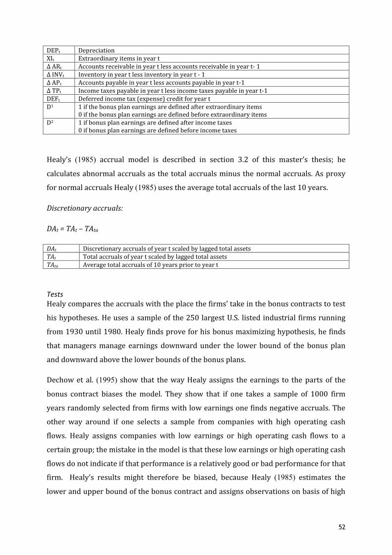
52

DEPt  Depreciation  XIt  Extraordinary items in year t ∆ ARt   Accounts receivable in year t less accounts receivable in year t‐ 1 ∆ INVt  Inventory in year t less inventory in year t ‐ 1 ∆ APt  Accounts payable in year t less accounts payable in year t‐1 ∆ TPt  Income taxes payable in year t less income taxes payable in year t‐1 DEFt  Deferred income tax (expense) credit for year t D1  1 if the bonus plan earnings are defined after extraordinary items 

0 if the bonus plan earnings are defined before extraordinary items D2  1 if bonus plan earnings are defined after income taxes 

0 if bonus plan earnings are defined before income taxes  

Healy’s  (1985)  accrual  model  is  described  in  section  3.2  of  this  master’s  thesis;  he 

calculates abnormal accruals as the total accruals minus the normal accruals. As proxy 

for normal accruals Healy (1985) uses the average total accruals of the last 10 years.  

Discretionary accruals: 

DAt = TAt – TAta 

DAt  Discretionary accruals of year t scaled by lagged total assets TAt  Total accruals of year t scaled by lagged total assets TAta  Average total accruals of 10 years prior to year t  

Tests Healy compares the accruals with the place the firms’ take in the bonus contracts to test 

his hypotheses. He uses a sample of the 250 largest U.S.  listed industrial  firms running 

from 1930 until 1980. Healy finds prove for his bonus maximizing hypothesis, he finds 

that managers manage  earnings  downward under  the  lower  bound  of  the  bonus  plan 

and downward above the lower bounds of the bonus plans.   

Dechow et al.  (1995)  show  that  the way Healy assigns  the earnings  to  the parts of  the 

bonus  contract  biases  the model.  They  show  that  if  one  takes  a  sample  of  1000  firm 

years randomly selected from firms with low earnings one finds negative accruals. The 

other  way  around  if  one  selects  a  sample  from  companies  with  high  operating  cash 

flows.  Healy  assigns  companies  with  low  earnings  or  high  operating  cash  flows  to  a 

certain group; the mistake in the model is that these low earnings or high operating cash 

flows do not indicate if that performance is a relatively good or bad performance for that 

firm.    Healy’s  results  might  therefore  be  biased,  because  Healy  (1985)  estimates  the 

lower and upper bound of the bonus contract and assigns observations on basis of high 

53

or  low  earnings  or  operating  cash  flow  without  knowing  whether  this  is  a  relatively 

good or bad performance for the firm.  

5.2.2 Bonus‐ based equity incentives and the Jones accrual model Holthausen et al. (1995) conduct a study that is similar to Healy (1985), the difference is 

that  Holthausen  et  al.  (1995)  use  the  Jones  and  modified  Jones  model  to  measure 

accruals  and  that  they  use  an  improved way  to measure  the  equity  incentives.  Their 

study examines  if  the same results are  found with a better accrual model and a better 

model to estimate the equity incentive. 

Model Holthausen et al. (1995) use the Jones and modified Jones model to measure accruals and 

find somewhat different results than Healy (1985). The Jones and modified Jones model 

are described in section 3.4 and 3.5 of this master’s thesis.  

To estimate  the equity  incentive Holthausen et  al.  (1995)  use  the  same measure Healy 

used (1985). They also assign observations to parts of the bonus schemes; like in Healy’s 

study observations can be under the lower boundary of the bonus scheme,  in between 

the boundaries of the bonus scheme or above the boundaries of the bonus scheme. The 

important difference is that Holthausen et al. (1995) have insider information about the 

bonus  schemes  to  their  disposal.  They  obtain  this  confidential  information  from  two 

human  resource management‐consulting  firms.  Therefore Holthausen  et  al.  (1995)  are 

able to use the real boundaries of the bonus plans, where Healy (1985) had to estimate 

this.  Therefore  Holthausen  et  al.  (1995)  have  a  more  precise  measure  to  assign 

observations  to  the  different  categories.  Holthausen  et  al.  (1995)  obtain  their  sample 

from two different human resources management consulting  firms,  they  test a  sample 

running from 1982 to 1984 and 1987 to 1991. 

Findings Holthausen  et  al.  (1995)  find  evidence,  like  Healy  (1985)  for  management  managing 

earnings downward above the upper limits of the bonus schemes, but they do not find 

evidence  for earnings being managed downward under  the  lower bound of  the bonus 

scheme.  Thereby  the  evidence  Holthausen  et  al.  (1995)  find  is  not  as  strong  as  the 

evidence  Healy  finds.  Holthausen  et  al.  (1995)  state  that  the  reason  for  this  weaker 

relation  is  due  to  the  different  models  used.  Healy  estimates  the  upper  and  lower 

bounds  of  bonus  plans  where  Holthausen  et  al.  (1995)  use  confidential  insider 

54

information  on  bonus  plans  to  assign  the  observations.  Holthausen  et  al.  (1995)  state 

that  the  method  used  by  Healy  (1985)  to  assign  observations  to  the  three  different 

categories has influenced his results. 

5.3 Equity incentives Where  the  early  research  on management  incentives  due  to  remuneration  incentives 

focused  on  bonus  plan‐based  incentives  more  recent  studies  have  examined  equity‐

based  management  incentives  like  I  use  in  this master’s  thesis.  In  the  next  section  I 

discuss  a  number  of  models  that  study  the  relation  between  equity  incentives  and 

earnings management. 

5.3.1 Equity incentives and the Jones accrual model Bergstresser and Philippon (2006) measure the relation between equity incentives and 

earnings management. They use an accrual model to measure earnings management and 

an incentive ratio as proxy for the total equity incentive.  

Expectations Bergstresser and Philippon (2006) expect that CEO’s manage earnings upwards in order 

to  maximize  the  gains  from  equity  incentives;  they  expect  that  CEO’s  whose 

remuneration  is  more  sensitive  to  the  company’s  stock  price  are  more  likely  to  use 

earnings management.  

Accrual model Bergstresser and Philippon  (2006) use the  Jones and Modified Jones model  to estimate 

the discretionary accruals. The Jones and modified Jones model are discussed in section 

3.2 and 3.3 of this master’s thesis. Bergstresser and Philippon (2006) use both the cash 

flow  method  as  the  balance  sheet  method  to  calculate  the  total  accruals,  how  these 

methods work is explained in section 3.7. Bergstresser and Philippon (2006) use a time‐

series model to estimate the non‐discretionary accruals. They use data back to 1979 to 

estimate the coefficients in the Jones model.  

Equity incentives Bergstresser and Philippon  (2006) examine the relation between equity  incentives and 

earnings management by estimating the relation between discretionary accruals and an 

incentive ratio. This ratio represents the sensitivity of the total CEO remuneration to a 

change in stock price. I discussed this incentive ratio in section 4.3.  

55

They also use this  incentive ratio adding the  calculated option delta  to  the  formula, as 

suggested  by  Core  and  Guay  (2002),  this  option  delta  is  discussed  in  section  4.3.This 

delta  is  calculated  using  the  Black‐Scholes‐Merton  formula,  and  indicates  the  relation 

between the share price and the value of  the options.  In the model without  the option 

delta  the  share  price multiplied with  the  number  of  options  is  used  as  proxy  for  the 

value  of  options.  When  using  this  proxy  one  assumes  that  the  option  delta  is  one. 

Bergstresser and Philippon (2006) find similar results with both these measures.  

Sample Bergstresser  and  Philippon  (2006)  test  the  relation  between  their  incentive  ratio  and 

discretionary accruals over a period from 1994 to 2000. The sample they use consists of 

publicly held firms, they split the sample in 4199 firm year observations with firms that 

have 1996 lagged assets above one million dollars and 4671 firm year observations with 

firms that have 1996 lagged assets below one million dollars. They obtain their data on 

CEO  remuneration  from  the  “execucomp”  database  and  obtain  information  used  to 

calculate accruals from the “compustat” database.  

Model Bergstresser and Philippon  (2006) examine the relation between equity  incentives and 

earnings management with the following equation.  

Absolute value of discretionary accruals =   +   × Incentive_Ratioi,t +  i,t × Controls +  i,t 

Bergstresser and Philippon  (2006)  use different  regressions  for  firms with  total  assets 

under  one  million  dollars  and  firms  with  total  assets  over  one  million  dollars. 

Bergstresser and Philippon (2006) winsorise all variables on the 1st and 99th percentiles. 

The  Controls  in  the  model  represents  a  set  of  control  variables  that  control  for  firm 

characteristics as size, leverage, firm age, and volatility of sales growth. Bergstresser and 

Philippon  (2006)  use  different  regressions  to  test  their  model  as  they  use  both  the 

absolute value of discretionary accruals and the absolute value of total accruals, and use 

accruals  calculated  with  cash  flow  information  and  accruals  calculated  with  balance 

sheet  information,  they  test  the  equity  incentive  in  two  versions:  one with  the option 

delta proposed by Core and Guay (2002) and one without this option delta. All methods 

lead to similar results.  

56

Findings Bergstresser and Philippon (2006) find that in firms where the CEO’s total remuneration 

is  more  sensitive  to  the  stock  price,  discretionary  accruals  are more  actively  used  to 

manage earnings.  

5.3.2 Equity incentives and analyst forecasts Cheng and Warfield (2005) examine the relation between equity incentives and earnings 

management. The equity incentives they examine are equity incentives that come from 

stock ownership and stock and options awarded. 

Cheng and Warfield (2005) measure earnings management as the likelihood of managers 

meeting or beating the analyst forecast; they compare this measure with their measure 

of  equity  incentives.  They  also  examine  if  managers  who manage  earnings  sell  more 

shares after meeting or just beating the analyst forecast. Besides the meeting or beating 

of  the  analyst  forecast  they  also  use  abnormal  accruals  as  measure  for  earnings 

management. The abnormal accrual part of their study is the part that is relevant for this 

thesis as accrual models are used in this master’s thesis as well.  

Expectations The first and main hypothesis of their study is: 

“The incidence of earnings management is positively related with equity incentives”.  

Besides the main hypotheses the second relation Cheng and Warfield (2005) examine is 

that: “firms with high equity incentives are more likely to sell shares in the future and 

that motivates these managers to engage in earnings management to increase the value 

of  the  shares  to  be  sold”. They  expect  that  there  is  a  difference  in  CEO’s who  receive 

persistent high equity incentives and CEO’s whose equity incentives are less persistent. 

They  expect  that  CEO’s whose  equity  incentives  are  less  persistent  are more  likely  to 

report surprisingly high or low earnings and that CEO’s whose incentives are persistent 

do  not  report  shock  earnings  but  more  constant  earnings.  Managers  who  have  high 

equity  incentives  over  a  long  period  of  time  are  expected  to  smooth  earnings,  and 

therefore not report shock earnings but a more constant amount of earnings. The third 

relation Cheng and Warfield predict is that managers sell more shares in the period after 

the announcement of earnings.  

57

Equity incentives As measure  for  equity  incentives Cheng and Warfield  (2005)  use  a  ratio  of  five  equity 

elements divided by the total outstanding shares of the firm. The fife elements of equity 

incentives  they  use  are:  “option  grants  in  the  current  period,  un‐exercisable  options 

(excluding  option  grants  in  the  current  period),  exercisable  options,  restricted  stock 

grants, and stock ownership.” They deflate these indicators by total outstanding shares 

of the firm. Cheng and Warfield (2005) measure the five different elements separately as 

well; however in most analyses the ratios of restricted stock grants are combined to one 

measure with share ownership and the option grants are combined to one measure with 

un‐exercisable options. Cheng and Warfield (2005) use these ratios because the benefit 

of possible gains due to increased short‐term stock prices is shared by all shareholders. 

Therefore  the  gain  acquired  by  the  CEO  is  proportional  to  the  ratio  of  the  equity 

incentives in the total shares outstanding.  

Equity incentives and earnings management measured with abnormal accruals Cheng and Warfield (2005) state that equity incentives can be an incentive to use income 

increasing accruals but that income smoothing incentives may lead to the use of income 

decreasing  accruals.  That means  that  the  relation  between  discretionary  accruals  and 

equity  incentives  is  positive  or  negative  depending  on  the  fact  which  of  the  two 

incentives is stronger (Cheng & Warfield, 2005).  

Cheng  and Warfield  (2005)  define  abnormal  accruals  as  the  difference  between  total 

accruals  and  normal  accruals.  They  estimate  the  normal  (non‐discretionary)  accruals 

with  the  cross‐sectional  version  of  the  Jones  (1991) model  as  described  in  section  3.4 

and 3.6.2 of this master’s thesis. Cheng and Warfield (2005) use the two digit SIC code to 

group  the  firms  into  industry  categories  and delete  all  industry  groups with  less  than 

seven observations.  

They  use  the  following  regression  to  estimate  the  relation  between  equity  incentives 

and earnings management: 

Abnormal accrualsi,t =  0 + ß Eq_incent,t +  1 sizei,t +  2 Leveragei,t + 3 Bonusi,t +  4 Riski,t +  5 

Growthi,t +  6 NOAi,t‐1 +  7 Litigationi,t+  8 Implicit claimi,t +  I,r 

Eq_incenti,t  Equity incentives measured in shares in the year t scaled by the number of 

outstanding shares. The measure contains five components explained above.  

58

Sizei,t  Natural logarithm of the market value of the firm at the end of the year Leveragei,t  Long term debt divided total assets at the end of the year Bonusi,t  Dummy variable is 1 for years that CEO’s are awarded a bonus and 0 if they are 

not awarded a bonus.  Riski,t  Market beta in fiscal year t estimated from weekly returns Growthi,t  The book to market ratio at the end of the fiscal year NOAi,t‐1  Net operating assets at the end of fiscal year t‐1 scaled by sales for fiscal year t‐1.  Litigationi,t  Dummy variable is one if the firm part of one of the following industries: 

pharmaceutical/biotechnology, computer, electronics, or retail and zero if the firm is in another industry. 

Implicit claimi,t  The implicit claim is proxied by the intensity of labour. This is calculated as one minus the ratio of gross property plant and equipment and total assets. 

 

Cheng  and Warfield  (2005)  add  the  above‐mentioned  control  variables  as  these might 

have an influence on the abnormal accruals. They add firm size to control for managers 

that tend to manage earnings to decrease political cost. Leverage is added to the model 

to control for the effects of debt covenants. To control for earnings management due to 

bonus‐related incentives Cheng and Warfield (2005) add a dummy variable that is 1 if a 

positive bonus  is  awarded and zero otherwise. Growth  is  added  to  the model because 

higher accruals are expected fast growing firms. 

CEO Trading Cheng  and  Warfield  (2005)  also  examine  the  share  sales  after  the  earnings 

announcement; they examine share sales in the first six months and second six months 

period  after  earnings  announcements. This data  is  obtained  from  the  SEC ownerships 

reporting file. Cheng and Warfield measure CEO trading as:  

Net CEO sales = Open market sales ‐ (Open market purchases + Options exercised). 

The net CEO sales are scaled by the firm’s market value at the end of the fiscal year.  

Earnings surprises A  third  measure  Cheng  and  Warfield  (2005)  use  are  earnings  surprises.  Earnings 

surprises are measured as: “the difference between the actual earnings and the earnings 

analysts predicted”, these earnings are measured per share. As measure for the analyst 

forecast Cheng and Warfield (2005) use the most recent analyst forecast within a three‐

months period before the earnings announcement.  

Sample Cheng and Warfield  (2005)  use a  sample  that  contains  companies with  information on 

stock‐  and  option‐based  remuneration  available  over  the  1993‐2000  period.  They 

59

obtain information on executive compensation from the standard & poor’s “execucomp” 

database. Cheng and Warfield use a sample of 9472 firm years. Financial institutions and 

firms  active  in  the  utilities  sectors  are  not  included  in  the  sample  because  these 

industries  are  highly  regulated  and  they  expect  that  these  managers  might  have 

different incentives to manage earnings.  

Findings Cheng and Warfield  (2005)  find that:  “CEO’s  that have high equity  incentives use more 

income‐increasing  abnormal  accruals  than  CEO’s  with  low  equity  incentives”.  This 

means that the incentive to increase earnings is stronger than the incentive to reserve 

earnings  for  the  future.  Reserving  earnings  for  the  future  would  be  in  line  with  the 

income‐smoothing  hypothesis.  Cheng  and  Warfield  (2005)  find  that  these  results  are 

mainly due to managers that have less persistent equity incentives, these managers have 

less  incentives  to  reserve  earnings  for  the  future  and  are  affected  less  by  accrual 

reversals. They state  that  if  the sample  is  split based on  the average ranking of equity 

incentives over the sample period they find that the relation between equity incentives 

and discretionary accruals  is not significant  for  firms with persistent equity  incentives 

and  that  the  relation  is  significant  for  companies  whose  equity  incentives  are  less 

persistent.  They  also  find  that  share  sales  by  CEO’s  increase  after  the  earnings  are 

presented in periods with high income increasing abnormal accruals. 

Using  their  other  indicator  for  earnings management  Cheng  and Warfield  (2005)  find 

that managers who have  persistent  high  equity  incentives  report  earnings  that  are  in 

line or slightly better than the analyst forecasts. Managers with consistently high equity 

incentives  are  less  likely  to  report  surprisingly  high  earnings.  This  is  consistent with 

what  they  expect,  managers  with  constant  high  equity  incentives  are  expected  to 

manage earning in a way that results in smooth earnings, as this provides them with the 

most profit from their current and future equity incentives.  

5.4 CEO and CFO equity incentives 

5.4.1 CEO and CFO equity incentives and accrual management Jiang, Petroni and Wang (2010) examine the relation between CFO equity incentives and 

earnings management, they compare their results with the relation between CEO equity 

incentives  and  earnings management  to  find which  relation  is  stronger.  By  doing  this 

they  continue  on  the  studies  of  Bergstresser  and  Philippon  (2006)  and  Cheng  and 

60

Warfield  (2005).  They  use  two  measures  for  earnings  management:  accruals  and  the 

likelihood  of  beating  analyst  forecast.  The  findings  found  with  the  accrual model  are 

most relevant for this thesis as an accrual model is used in this master’s thesis as well.  

Expectations Jiang  et  al.  (2010)  expect  that CFO equity  incentives have more  influence on  earnings 

management  than  CEO  equity  incentives.  To  examine  this  they  measure  the  relation 

between  equity  incentives  and  earnings  management  for  the  CEO  and  the  CFO 

separately and they also measure the joint relation.  Jiang et al. (2010) also expect that 

the Sarbanes Oxley act has led to a weakening in the relation between equity incentives 

and earnings management, therefore they measure these relations in the period prior to 

the Sarbanes Oxley legislation and the period after the Sarbanes Oxley legislation. 

Equity incentives As measure  for  equity  incentives  Jiang  et  al.  (2010)  use  the  equity  incentive  ratio  by 

Bergstresser  and Philippon  (2006).  This  ratio  is  described  in  section 4.3 of  this  thesis. 

Kim et al. (2011) use this measure as well. Kim et al. (2011) separate the equity incentive 

ratio in an option incentive ratio and a stock incentive ratio, Jiang et al. (2010) do not do 

this,  they  use  the  total  equity  incentive  ratio.  They  add,  like  Kim  et  al.  (2011)  and 

Bergstresser and Philippon (2006) do, the option delta to the model as proposed by Core 

and Guay (2002). The ratio contains the value of: the shares a manager owns, the newly 

granted options, unexercised‐exercisable options, and un‐exercisable options.  

Accrual model Jiang  et  al.  (2010)  estimate  the  relation  between  equity  incentives  and  earnings 

management using accrual models.  

They  calculate  the  total  accruals  as  the  “difference  between  earnings  before 

extraordinary  items,  scaled by  lagged  total assets”.  In  this way  they calculate  the  total 

accruals using cash flow data as described in section 3.7 of this master’s thesis.  

With the total accruals they calculate the discretionary accruals. They use the Forward 

looking  Jones  model  by  Dechow  et  al.  (2003)  to  calculate  discretionary  accruals,  this 

model is discussed in section 3.9 of this master’s thesis.  

TAi,t=  1 +  2((1+K) ∆salesi,t ‐ ∆ARi,t) +  3PPEt +  4 (TAi,t,‐1/ Ai,t‐2) +  5 GR_salesi,t  

   

61

TA  Total accruals in the current year of firm i, scaled by year t‐1 total assets. ∆sales     Change in sales, scaled by year t‐1 property plant and equipment ∆AR  The change in accounts receivable, scaled by year t‐1 total assets.   K  The slope coefficient from a regression of ∆AR on ∆sales PPE  Gross property plant and equipment TAi,t,‐1/ Ai,t‐2  Total accruals from the year before the current scaled by total assets of two years ago for 

firm i. GR_sales  The change in sales for firm i, from year t to t+1, scaled by year t sales.  

 

Jiang  et  al.  (2010)  calculate  the  discretionary  accruals  by  deducting  the  non‐

discretionarily  accruals  from  the  total  accruals.  They  use  the  absolute  value  of 

discretionary accruals in their final analysis.  

Final model With  the absolute value of discretionary accruals and  the equity  incentives  Jiang et al. 

(2010) estimate the following model: 

Absolute value discretionary accruals =  0 +  1 incentive ratio +   controls +   

Jiang et al.  (2010) use  the absolute value of  total and discretionary accruals  instead of 

the normal value as they expect that equity incentives increase extreme accruals. They 

control  for variables as:  firm size, a dummy  for  firm age,  the volatility of  sales growth 

and the leverage.  

Sample The  sample  Jiang  et  al.  (2010)  use  consists  of  S&P  1500  firms  that  are  part  of  the 

“execucomp” database and have data for CEO and CFO compensation available. They find 

a total of 17542 firm years with the data available on compensation of the CEO and the 

CFO. They test their sample over the period from 1993 to 2006. 

Findings Jiang et al. (2010) find that there is a positive relation between both CEO and CFO equity 

incentives  in  the  pre‐Sarbanes  Oxley  1994‐2000  period.  The  relation  for  CFO  equity 

incentives they find is stronger than the relation for CEO equity incentives. In the post‐

Sarbanes Oxley period they do not  find a positive relation between CEO or CFO equity 

incentives  and  earnings  management.  In  the  period  after  the  implementation  of  the 

Sarbanes  Oxley  legislation  they  even  find  a  negative  relation  between  CFO  equity 

incentives  and  earnings management.  Jiang  et  al.  (2010)  contribute  to  the  research of 

Cheng and Warfield  (2005)  and Bergstresser and Philippon  (2006) by showing  that  the 

62

relation between CFO equity incentives and earnings management is stronger than the 

relation between CEO equity incentives and earnings management. They also show that 

this  relation  changes  for  a  pre  and  post‐Sarbanes  Oxley  sample.  In  the  post‐Sarbanes 

Oxley  sample  they  even  find  a  negative  relation  between  CFO  equity  incentives  and 

earnings  management.  This  is  possibly  due  to  the  fact  that  in  the  period  after  the 

introduction  of  the  Sarbanes  Oxley  act  the  markets  reacted  negatively  to  positive 

earnings surprises if the firms’ management has high equity incentives. 

5.4.2 CEO and CFO equity incentives and crash risk Kim,  Li  and  Zang  (2011)  examine  the  relation  between  CEO  and  CFO  equity 

compensation  and  firm  crash  risk.  They  find  proof  that  the  sensitivity  of  the  CFO’s 

compensation to the stock price is positively related to firm’s crash risk. They however 

do not find positive evidence of the impact of the sensitivity of the CEO’s compensation 

and crash risk. 

Expectations Kim et al. (2011) predict to find a positive relation between equity incentives and crash 

risk. They  test whether  this  relation  is  stronger  for  the CFO or  for  the CEO. They also 

expect  that  options  have  a  more  powerful  impact  on manager’s  behavior  than  stock 

based incentives.  

Crash risk  Kim et al. (2011) examine the relation between equity incentives and crash risk.  

Kim et al. (2011) estimate the firm‐specific weekly returns for each firm and year; they 

need this measure to be able to measure the firm specific crash risk. They define crash 

weeks in a given fiscal year for a given firm, as those weeks in a year where the company 

experiences weekly returns 3.2 standard deviations below the mean.  

Their  first  measure  of  crash  probability  is  a  dummy  that  is  1  in  years  where  firms 

experience  one  or  more  crash  weeks  and  zero  in  years  where  the  firms  do  not 

experience crash risk.  

The second measure of crash risk they use is the negative conditional return skewness: 

“This is estimated by taking the negative of the skewness of firm‐specific weekly returns 

for each sample year and dividing that by the standard deviation of firm‐specific weekly 

returns raised to the third power”. 

63

The third measure of crash risk Kim et al. (2011) use is calculated by “separating all the 

weeks with firm‐specific weekly returns below the annual mean from weeks with firm‐

specific returns that are higher than the yearly mean. They then calculate the standard 

deviation for each of these subsamples separately. The final measure is the logarithm of 

the  ratio  of  the  standard  deviation  in  the  weeks  with  a  mean  below  average  to  the 

standard deviation of the weeks above average.”  

Equity incentives Kim  et  al.  use  the measure  proposed  by  Bergstresser  and  Philipon  (2006)  to  estimate 

equity incentives. This measure is discussed in section 4.3 of this master’s thesis. They 

first  calculate  ONEPCT  this  is  the:  “dollar  change  in  the  value  of  an manager’s  option 

holdings  that would come  from a one percentage point  increase  in  the company stock 

price”. They also calculate this measure for the stock holding 

The difference with Bergstresser and Philippon (2006) is that they calculate this measure 

for  both  option  and  stock  holdings  together.  Kim  et  al.  (2011)  calculate  this  measure 

separately for the option and stock holdings to be able to test if the influence of option 

or  stocks  is  stronger.  Kim  et  al.  (2011)  estimate  ONEPCT  with  the  option  delta  as 

proposed by Core and Guay. The option delta is explained in section 4.3. 

Sample The  sample  Kim  et  al.  (2011)  use  consists  of  US‐based  firms  obtained  from  the 

“Compustat  Executive  Compensation”  database.  Their  sample  runs  from 1993  to  2009. 

They  delete  observations  with  missing  data  in  the  “compustat”  database  and  in  the 

Research  in  Security  Prices  databases.  They  also  exclude  firms whit  a  year‐end  share 

price that is lower than 1 dollar. The sample consists of 29638 firm year observations.  

Main regression Kim  et  al.  estimate  the  relation  between  crash  risk  and  equity  incentives  with  the 

following regression: 

CrashRisk =  o +  1 × Incentive +   × Control Variables +   

Kim et al. (2011) use the measure of the dependent variable in year t and the measure of 

the  independent variable  in year t‐1.   They add a number of control variables  that are 

seen  as  possible  predictors  of  the  crash  risk.  They  also  control  for  abnormal  accruals 

calculated  with  the  modified  Jones  model;  this  is  done  to  ensure  that  the  relation 

64

between  equity  incentives  and  crash  risk  is  not  due  to  managers  using  accrual 

accounting, because they expect that accruals accounting increases crash risk. 

Findings Kim et al.  (2011)  find  that CEO and CFO stock  incentives are not related  to  the  future 

crash risk. But  that CEO and CFO option  incentives are positively related to crash risk. 

The relation for the CEO is however less significant than the relation for the CFO. They 

find  that:  “CFO  option  incentives  dominate  CEO  option  incentives  in  predicting  the 

future crash risk”. Kim et al.  (2011) use  like  Jiang et al.  (2010) both  the CEO and CFO 

equity  incentives.  They  find  that  there  is  no  relation  between  stock  incentives  and 

earnings management  but  a  positive  relation  between  option  incentives  and  earnings 

management.  They  find  this  relation  over  the  period  1993  to  2009.  These  findings  in 

combination with  the  Jiang  et  al.  (2010) paper  leads  to  a  number  of  things  to  further 

examine. I discuss this in the next chapter. A possible problem with the study by Kim et 

al. (2011) is that it covers the 1993‐2009 period, this period contains a period before the 

implementation of the Sarbanes Oxley act and a period after the Sarbanes Oxley act. This 

might contaminate their research as Jiang et al. (2010) show that the relation between 

equity  incentives  and  earnings  management  is  different  before  and  after  the 

implementation of Sarbanes Oxley. This might also hold for the relation between equity 

incentives and crash risk. 

5.5 Summary This  chapter  discusses  empirical  research  on  equity  incentives  and  earnings 

management. The first part discusses research on remuneration incentives. The first of 

the remuneration papers is the paper by Healy (1985), he finds evidence for his bonus 

maximizing  hypothesis.  Healy  (1985)  finds  that  CEO’s  manage  earnings  downward 

under  the  lower  boundary  of  bonus  plans  and  above  the  upper  boundaries  of  bonus 

plans.    The  article  by  Holthausen  et  al.  (2005)  is  the  second  remuneration  article 

discussed.  Holthausen  et  al.  (1995)  find  a  little  different  results,  they  find  like  Healy 

(1985)  evidence  for  managers  managing  earnings  downward  from  above  the  upper 

boundary of bonus plans but they do not find evidence for managers managing earnings 

downwards below the lower bound of the bonus plan.  

 

The  second  part  of  this  chapter  discusses  three  papers  that  examine  the  relation 

between  equity  incentives  and  discretionary  accruals.  Bergstresser  and  Philippon 

65

(2006)  find evidence  for a positive relation between discretionary accruals and equity 

incentives.  As  measure  for  equity  incentives  they  use  a  ratio  that  measures  the 

sensitiveness  of  CEO  income  to  the  stock  price  of  the  company.  Cheng  and Warfield 

(2005)  measure  the  relation  between  equity  incentives  and  CEO’s  meeting  or  just 

beating  the  “analyst  forecasts”  and  the  relation  between  equity  incentives  and 

discretionary accruals. Cheng and Warfield (2005) find that CEO’s who have high equity 

incentives use more income increasing abnormal accruals. They also find that managers 

with persistent high earnings are less  likely to present surprisingly high earnings than 

managers with less persistent equity incentives. And they find that CEO’s with persistent 

high earnings are likely to meat or just beat the “analyst forecasts”.  

 

The  third  part  of  this  chapter  discusses  studies  that  measure  the  relation  between 

equity  incentives and earnings management  for both  the CEO and  the CFO.  Jiang et al. 

(2010) find that there is a positive relation between both CEO and CEO equity incentives 

and  earnings management.  They  find  that  the  relation between CFO  equity  incentives 

and earnings management is stronger than the relation between CEO equity incentives 

and earnings management. They find these positive relations in a sample running before 

the introduction of the Sarbanes Oxley act;    in a sample running in the period after the 

introduction  of  the  Sarbanes  Oxley  act,  they  find  no  positive  relation  between  equity 

incentives and earnings management.   Kim et al. (2011) measure the relation between 

equity incentives and crash risk. Kim et al. (2011)  examine if this relation is different for 

CEO  equity  incentives  or  CFO  equity  incentives.    They  find  that  the  relation  between 

equity  incentives  and  crash  risk  is  stronger  for  the  CEO  than  for  the  CFO.  They  also 

examine if there is a difference between stock and option based equity incentives. They 

find no positive relation between stock‐based equity incentives and crash risk, they do 

find a positive relation between option based equity incentives and crash risk.  In the next chapter I present my expectations and the hypotheses of my master’s thesis. 

These expectations are based on the prior research I discussed in this chapter.  

66

Chapter 6 Hypothesis 

6.1 Hypothesis 1 I expect to find a positive relation between earnings management and equity incentives. 

I expect that when the compensation of an executive is more sensitive to the stock price 

he  uses  earnings  management  to  increase  the  performance  of  the  company.  Prior 

research  shows  evidence  for  this  relation  as well.  Examples  of  these prior  studies  are 

Cheng and Warfield  (2005) and Bergstresser and Philippon (2006). They find a positive 

relation  between  accrual‐based  earnings  management  and  measures  for  equity 

incentives. 

H1: There is a positive relation between earnings management and equity incentives. 

6.2 Hypothesis 2 Because the main job of a CFO is to take care of the financial administration I expect that 

the CFO has more  influence on earnings management  than  the CEO has. Providing  the 

CFO  with  a  compensation  that  is  highly  sensitive  to  the  stock  price  of  the  firm  is 

therefore,  in  my  opinion,  asking  for  trouble.  Because  the  CFO  is  the  manager  that  is 

responsible for composing the financial statements and for making accrual decisions it is 

very easy  for him to manage earnings. As the CFO can manage earning with less effort 

than  the  CEO  the  CFO  could  be  tempted  to  use  earnings management  quicker  than  a 

CEO. This expectation is supported by the findings of Jiang et al. (2010) , discussed in the 

previous  chapter.  They  find  a  positive  relation  between  discretionary  accruals  and 

earnings management;  they  find a stronger relation  for CFO equity  incentives  than for 

CEO equity incentives.  

H2: The positive relation between earning management and equity  incentives  is stronger 

for CFO’s than for CEO’s 

6.3 Hypothesis 3 I also expect to find a stronger relation for option‐based incentives than for share‐based 

incentives. This is due to the character of options as short‐time incentive. It is easy for 

management  to  make  quick  gains  with  options  in  years  where  many  options  can  be 

exercised.  Due  to  the  reversing  character  of  accruals  they  are  well  suited  to  use  in 

combination with short‐term  incentives. This  is because when using accruals earnings 

can  only  be  managed  upwards  for  a  limited  amount  of  time,  after  this  accruals  will 

67

reverse.  This  suits  the  character  of  options,  as  earnings  only  have  to  be  managed 

upwards for a short period of time to be able to exercise the options at a good price. Kim 

et  al  (2011)  find  that  there  is  no  relation  between  stock‐based  equity  incentives  and 

crash risk over the 2003‐2009 period but they do find that there is a relation between 

option‐based  equity  incentives  and  crash  risk.  This  supports my  expectation  to  find  a 

stronger  relation  between  option‐based  equity  incentives  and  earnings  management 

than  between  stock‐based  equity  incentives  and  earnings  management.  Cheng  and 

Warfield (2005) find that managers with less persistent equity incentives are more likely 

to  present  surprisingly  high  earnings  than  managers  with  more  persistent  equity 

incentives.  As  option  incentives  are  less  persistent  than  stock‐based  equity  incentives 

this  leads  to  the  expectation  that  option‐based  equity  incentives  are  short  time 

incentives  and  lead  to management managing  earnings  up  in  periods when  there  are 

many option‐based incentives available.  

H3:  The  relation  between  equity  incentives  and  earnings  management  is  stronger  for 

option‐based incentives than for share‐based incentives. 

6.4 Hypothesis 4 I expect to find a positive relation between earnings management and equity incentives. 

This  is  in  line with  the  findings of  Jiang et  al.  (2010)  in  their  study;  they  find  that  the 

relation  between  equity  incentives  and  discretionary  accruals  weakens  in  the  period 

after the implementation of the Sarbanes Oxley act. I expect to find similar results. I also 

examine if this relation is different for option‐based and share‐based incentives. I expect 

to  find  that  the  decline  of  this  relation  is  stronger  for  the  short‐term  option‐based 

incentives  than  for  the  share‐based  incentives.  As  to  my  opinion  these  short‐term 

option‐based  incentives  are more  sensitive  for  opportunistic  use. Managers  can more 

easily manage earnings upwards  for a  short period of  time  than  they can  for a  longer 

period.  Another  reason  that  the  positive  relation  between  earnings management  and 

option‐based  incentives  might  have  declined  is  that  the  market  reacts  negatively  to 

positive  earnings  surprises  in  the  period  after  the  Sarbanes  Oxley  act  has  come  into 

effect, this  is shown by Kothari et al. (2006). Earnings growth to maximize the rewards 

from option incentives is therefore not effective anymore if the earnings growth comes 

by surprise. Steady long‐term growth however may still lead to a positive relation from 

the markets. Another possible explanation why the relation for option‐based incentives 

68

should decline faster than the relation for stock‐based incentives is that firms may have 

become more careful awarding managers which options‐based  incentives, because  the 

short  term  incentives may have caused harmful earnings management, as well as  that 

option‐based  incentives do not  succeed  to align  the  interests of management with  the 

owners of the firm as well long term incentives do. As stockholders are often better off 

by long‐term growth than short‐term earnings shocks, this applies in particular for large 

institutional  shareholders  like  pension  funds.  Another  reason  is  that  option‐based 

incentives might have become less popular due to the effect that option‐based incentives 

lead  to risk‐seeking behavior as  I explained  in  the  introduction  to  this master’s  thesis. 

The risk seeking management might not be in line with the interest of stockholders.  

H4:  The  positive  relation  between  equity  incentives  and  earnings management  declines 

after the major accounting scandals of the early 2000s, this decline is stronger for option‐

based incentives. 

69

Chapter 7 Research design and methodology 

7.1 introduction This  chapter  describes  the  empirical  research  of  this master’s  thesis;  it  explains what 

methods are used to obtain the results presented in the next chapter. As described in the 

introduction  of  this  master’s  thesis  I  want  to  measure  the  relation  between  equity 

incentives and earnings management and thereby focus a possible different relation for 

CEO and the CFO, and different effects of option‐based and stock‐based incentives. I test 

this  relation  over  a  ten‐year  period  running  from  1999  to  2009.  I  choose  this  period 

because it contains accounting scandals that have had a major impact on the accounting 

world.  I use an accrual model to measure earnings management and an incentive ratio 

to measure the equity  incentive. This chapter will  first describe the accrual model and 

the incentive ratio I use and then describe the sample used.  

7.2 Accrual model To measure earnings management  I use  the  linear  cross‐sectional performance model 

by Kothari et al. (2005) I described this model in section 3.12. I use this model because if 

one  measures  earnings  management  caused  by  equity  incentives,  it  is  especially 

important  to  control  for  firm  performance  and  that  is  what  the  Kothari  et  al.  (2005) 

model does. The goal of the earnings management is to enhance firm performance, there 

is  a  correlation  between  firm  performance  and management  compensation  (Ronen &

Yaari, 2008),  therefore  controlling  for  firm  performance  is  important  when  using 

earnings management in combination with equity incentives.  

I  use  the  linear model  introduced  by  Kothari  et  al.  (2005)  rather  than  the  non‐linear 

Kothari et al. (2005) model, as there is no reliable way of matching at my disposal for this 

sample. Such a method would for instance be available if one wants to measure earnings 

management around a  certain event, where one group experiences  such an event and 

another group of companies does not,  it  is  than possible  to match companies  from the 

first group with companies from the second group. This is however not possible in my 

research design, therefore I will use a linear approach.  The advantage of the non‐linear 

model  is  that  it mitigates  the non‐linearity problem of  the  return on  assets.  Ye  (2007) 

however introduces another way to mitigate the non‐linearity problem in the return on 

assets, he winsorizes the return on assets to normal values between ‐0.1 and 0.3. I use 

70

the method Ye (2007) proposes, to mitigate the possible non‐linearity problem in return 

on assets.  I also, winsorize the accruals and  incentive rations on  first and ninety‐ninth 

percentile to exclude effects of extreme performance. The model is estimated in a cross‐

sectional  way  because  a  time‐series  model  assumes  an  earnings  management  free 

estimation period, which is not a realistic assumption for this research design. The two 

digit sic codes are used to divide the companies into their industry groups in order to be 

able to perform the cross‐sectional test. I use the two digit sic code instead of the full sic 

code to obtain larger groups, because larger groups lead to better results.  The hindsight 

of having larger groups is that separating the firms into groups is done less precise: the 

groups  are  larger  therefore  firms  are  put  into  groups  with  firms  that  can  be  quite 

different.  

I calculate the total accruals using cash flow information. Hribar and Collins (2002) show 

in  their  study  that  this  leads  to  better  results  around  non‐articulation  events.  Total 

accruals are calculated as net income minus cash flow from operations. 

TAi,t = (NIi,t – CFOI,t)/ A i,t ‐1 

TAi,t  Total accruals calculated with cash flow information of firm I at time T scaled by lagged total assets 

NI i,t  Bottom line net income CFO i,t  Operating cash flows  A i,t ‐1  Total Assets  I use the total accruals to estimate the coefficients in the formula for nondiscretionary 

accruals.  I  estimate  the  coefficients  using  the  cross‐sectional  linear  version  of  the 

Kothari et al. (2005) model: 

TAi,t =  0 +  1 (1/Ai,t ‐1)+  2( REVi,t ‐   ARi,t )/Ai,t‐1) +  3 (PPEi,t/ Ai,t‐1) +  4 ROAi,t‐1 

TAi,t  Total accruals scaled by lagged total assets REVi,t  The change in revenue ARi,t  The change in accounts receivable  PPEi,t  Gross property plant and equipment  ROAi,t‐1  Lagged rate of return on assets Ai,t‐1  Total assets  

With the estimated coefficients the non‐discretionary accruals can then be calculated: 

NDAi,t=  0 +  1 (1/Ai,t ‐1)+  2(  REVi,t ‐   ARi,t )/Ai,t‐1) +  3 (PPEi,t/ Ai,t‐1) +  4 ROAi,t‐1 

71

NDAi,t  Non‐discretionary accruals scaled by lagged total assets REVi,t  The change in revenue ARi,t  The change in accounts receivable  PPEi,t  Gross property plant and equipment  ROAi,t‐1  Lagged rate of return on assets Ai,t‐1  Total lagged assets  

Once  the  non‐discretionary  accruals  are  calculated  the  discretionary  accruals  can  be 

derived: 

DAi,t = TAi,t – NDAi,t  DAi,t  Discretionary accruals scaled by lagged total assets TAi,t  Total accruals scaled by lagged total assets  NDAi,t  Non‐discretionary accruals scaled by lagged total 

assets   The discretionary accruals are used as measure  for earnings management and will be 

compared with equity incentives to examine the relation between equity incentives and 

earnings management and thereby answering the research questions. 

7.3 Measure for equity incentives In  this master’s  thesis  I want  to measure  the  relation  between  earnings management 

and equity  incentives. As measure  for  the  incentive created by stock and option‐based 

remuneration  I  use  effect  of  a  change  in  the  stock  price  on  total  remuneration.  This 

measure  is  based  on  the  measure  used  by  Bergstresser  and  Philippon  (2006),  it  is 

however different than the measure they use.  

The  modification  is  that  the  option  part  of  the  formula,  uses  the  estimated  value  of 

options, were Bergstresser and Philippon  (2006) use  the number of options multiplied 

by  the  share price. With  this Bergstresser and Philippon  (2006)  implicitly assume  that 

the when  the  stock price  changes  the value of options  change  in  the  same way as  the 

value of stocks. This is however a quite rough assumption as the valuation of options is 

more complex.  

As  explained  in  the  first  chapter  of  this master’s  thesis,  options  create  a  short‐term 

incentive for managers. This is due to the fact that options have an expiration date, after 

this  date  they  are  valueless. Managers  are  triggered  to maximize  the  value  of  options 

72

before the expiration date. In this way they are able to sell or exercise the options for the 

best price possible.  

As measure for the effect of the change in the value of a CEO’s stock or options portfolio 

due to a one percent change in the stock price, I use the following measure.  

EQVALi,t = 0.01 × PRICEi,t × SHARESi,t + 0.01 × OPTIONVALi,t 

EQVAL  The equity value ratio measured as the dollar change in the value of a CEO’s stock and options holdings that would come from a one‐percentage point increase in the company stock price. 

PRICE  Company share price SHARES  Number of shares held by the executive OPTIONVAL  Value of options held by the executive + value realized on options exercise during the 

year.  

This equity value ratio differs from the ratio used by Bergstresser and Philippon (2006) 

on  one  important  point  as  this  ratio  uses  the  estimated  value  of  options  +  the  value 

realized on option  exercise during  the  year. Where Bergstresser  and Philippon  (2006) 

use the number of options multiplied by the share price. It still measures the change in 

value of the stock and option portfolio held by the executive due to a one percent change 

in the firms’ stock price as the option value also contains the stock price of the firm. The 

value  realized  on  option  exercise  is  added  to  the  model,  as  this  value  is  part  of  the 

incentive for an executive to manage earnings during a year. The intrinsic value of the 

options  is  derived  from  the  “compustat  execucomp”  database  and  is:  the  estimated 

intrinsic value of the unexercised exercisable options as reported by the company6. The 

non‐exercisable options are not included in the model as they are irrelevant in the short 

term.    The  options  will  automatically  be  included  in  the  model  from  the  year  they 

become  exercisable,  because  from  that moment  they  directly  influence  the  executives 

income.  

This measure improves the Bergstresser and Philippon (2006) measure, as the change in 

the value of the options is measured more precise. Because the method Bergstresser and 

Philippon (2006) use is a rough estimate for the value of options.  

6 From 2006 onwards this measure is changed in the intrinsic value of exercisable options, calculated based on the difference between the exercise price of the options and the close price of the company’s primary issue of stock.   

73

With  the  calculated  equity  value  ratio  the  incentive  ratio  is  calculated.  This  incentive 

ratio  represents  the:  “hypothetical  CEO’s  total  compensation  that would  come  from  a 

percentage  point  increase  in  the  value  of  the  equity  of  the  firm”  (Bergstresser &

Philippon, 2006).  

INCENTIVE RATIO i,t = EQVAL i,t/(EQVAL i,t + SALARY i,t + BONUS i,t) 

INCENTIVE RATIO  The hypothetical CEO’s total compensation that would come from a one percentage point increase in the value of the equity of the firm 

EQVAL  The equity value ratio measured as the dollar change in the value of a CEO’s stock and options holdings that would come from a one‐percentage point increase in the company stock price. 

SALARY  The fixed salary awarded to the executive BONUS  The cash bonus awarded to the executive  

This incentive ratio is calculated in three different ways, the first one as described above 

taking  into  account  total  equity  incentives.  The  other  two  measures  focus  on  the 

influence of option or stock‐based equity incentives. In those models the EQVAL ratio in 

the nominator is calculated using only the option part of the EQVAL formula or only the 

stock part of the EQVAL formula. In that way the influence from the options‐ and stock‐

based incentives can be measured separately. 

7.4 Estimating the relation between earnings management and equity incentives To answer the research questions I examine the relation between earnings management 

and equity incentives. Therefore the incentive ratios and the discretionary accruals are 

compared in a regression. In order to provide a more detailed view of this relation I use 

different regressions using data for the CEO, the CFO and both of them together. Each of 

the  three  tests  are  carried out  three  times  each;  once with  the  total  equity  incentives 

ratio, once the option incentive ratio and once with the stock incentive ratio.  

DAi,t   = α 0 + α1 × INCENTIVE RATIO + αx + Controls  

DAi,t    Absolute value of discretionary accruals scaled by lagged total assets INCENTIVE RATIO  The hypothetical CEO’s total compensation that would come from a one 

percentage point increase in the value of the equity of the firm Controls  Control variables, discussed in descriptive statistics 

7.5 Sample In this section I discuss the sample selection. The sample consists of firms listed in the 

United States that are part of the S&P 500 index. The sample period is 1999 until 2009, I 

74

use  this  period  because  it  covers  important  accounting  scandals,  years  before  these 

scandals and  the years after  these  scandals,  I  choose  to  take a  longer period after  the 

scandals as I expect that it will take some time for the dust to settle after these events. 

The companies need to meet the following requirements to be included in the sample: 

‐ The firm is part of the S&P 500 

‐ The firm does not have any missing values for the variables required 

‐ Firm total assets are more than one million dollars. 

‐ Firms are in industry groups of ten firms or more 

The  requirement  that  firm  total  assets  have  to  be  more  than  one  million  dollars  is 

because  firm  total  assets  are  used  as  scaling  variable.  Therefore  a  small  value  may 

generate  unusual  observations  that  are  of  little  significance  (Ye, 2007).  The  data  to 

estimate  the  accruals  is  derived  from  the  comp  stat  database.  Data  about  executive 

remuneration is derived from the “execucomp” database.  

7.6 Descriptive statistics The sample used in this study contains information derived from the “compustat North 

America” database and the “execucomp” database. The variables used for this study are 

described in appendix 2.   

For tests over the total research period running from 1993 until 2009 a total of 12587 

firm  years  are  included  in  the  sample.  For  the  period  prior  to  the  introduction  of  the 

Sarbanes Oxley act 3168 firm years are included in the sample. In the period from 2003 

until 2009 8346 firms years are included in the sample.   

To identify the CEO’s in the database the variable “annual CEO flag” was used, this points 

out which of the executives in the database was CEO of the firm in the specific firm year. 

Such a variable is available as well for the function of CFO This variable however is not 

suited for my research design as this variable is not introduced until 2006. Therefore the 

CFO’s have to be identified in different way. To identify the CFO the variable “Title_Ann” 

is  used. This  variable  indicates  the name of  the  function of  the  executive  per  year. To 

identify  the  CFO’s  all  executives  are  classified  as  CFO  if  their  title  contains  one  of  the 

75

following  words:  CFO,  chief  financial  officer,  treasurer,  controller,  finance,  vp‐finance 

and administrative. This method is identical as the method used by Kim et al. (2011). 

7.6.1 Calculation of discretionary accruals  Appendix  2a  shows  the  descriptive  statistics  for  the  calculation  of  the  discretionary 

accruals. The discretionary accruals are calculated as described in section 7.2. First the 

total  accruals  and  independent  variables  are  used  in  a  regression  to  estimate  the 

coefficients. Then the coefficients are used in the formula to calculate non‐discretionary 

accruals.  With  the  non‐discretionary  accruals  the  total  accruals  are  calculated  by 

deducting the non‐discretionary accruals from the total accruals. The definitions of the 

variables  used  to  calculate  discretionary  accruals  are  included  in  appendix  2b.The 

average  of  the  total  accruals  is  similar  to  the  average  of  the  total  accruals  found  by 

Bergstresser  and  Philippon  (2006)  in  their  study.  They  find  a  mean  of  0,062  for  the 

absolute value of total accruals for a sample of companies with lagged 1996 assets above 

1  billion  dollars.  Their  standard  deviation  is  lower  than  the  standard  deviation  in my 

sample:  0,054  compared  to  0,075.  This  difference  is  probably  due  to  the  fact  that  the 

Bergstresser and Philippon (2006) sample only contains firms with lagged 1996 assets 

above 1 billion dollar; my sample contains firms with total assets above and below one 

billion dollars. The study by Bergstresser and Philippon (2006) also includes a sample of 

firms with  total  assets  below 1  billion  dollar,  for  that  sample  the  average  of  the  total 

accruals are higher: 0,089 and the standard deviation is higher as well: 0,271. This could 

explain  a  higher  standard  deviation  for my  sample because  the  sample  I  use  contains 

both  firms with  assets  above  1  billion  dollar  and  firms with  assets  below  one  billion 

dollar. This is supported by Kothari et al. (2005), they state that accruals of small firms 

are more volatile than accruals of large firms. 

Compared to Jiang et al. (2010) the average of the total accruals in this master’s thesis 

are  a  bit  lower.  Jiang  et  al.  (2010)  use  a  sample  of  S&P  1500  firms  and  they  find  an 

average of  the  total  accruals  of  0,082  and a  standard  deviation of  0,078.  Their higher 

average of the total accruals could be explained by the fact that their S&P 1500 sample 

contains  more  small  firms  than  the  S&P  500  sample  I  use;  of  the  two  samples 

Bergstresser  and  Philippon  (2006)  use,  the  sample  of  smaller  firms  has  higher 

discretionary accruals as well. 

76

The discretionary accruals I find are a bit lower than the average discretionary accruals 

Bergstresser  and  Philippon  (2006)  find;  0,031  in my  study  compared  to  0,041  in  the 

study by Bergstresser and Philippon (2006). A possible explanation for this difference is 

that  the  discretionary  accruals  in  this  master’s  thesis  are  estimated  using  a  linear 

Kothari  model  while  Bergstresser  and  Philippon  (2006)  use  the  Jones  and  modified 

Jones models.  Another possible  explanation  is  that  Bergstresser  and Philippon  have  a 

different sample period; their sample runs from 1993 to 2001 and my sample runs from 

1999  to  2009.  Chart  1  shows  that  the  average  discretionary  accruals  in  this master’s 

thesis  never  reach  the  average  value  Bergstresser  and  Philippon  (2006)  find.  The 

average discretionary accruals Jiang et al. (2010) find are higher than the discretionary 

accruals in this master’s thesis, Jiang et al. (2010) find average discretionary accruals of 

0,072 compared to the average of 0,031 in my sample. This difference is probably due to 

the fact their sample contains S&P 1500 firms, that means that their average firm will be 

smaller than the average firm in my sample.  

 

Chart 1 shows the development of the average value of absolute discretionary accruals 

over the sample period used in this master’s thesis. It shows that the average absolute 

value of discretionary accruals declines after 2002, the year in which the Sarbanes Oxley 

act was introduced. It shows a peak again in 2008, in 2009 it returns to a value around 

the normal value for the period 2003‐2007. The peak in 2008 could be explained by the 

Chart 1 average absolute discretionary accruals 

77

financial crises that started with the bankruptcy of Lehman Brother in September 2008.  

Due to this crisis many firms had to revalue their assets and liabilities, this could explain 

the relatively high discretionary accruals in 2008.   

7.6.2 Descriptive statistics of the equity incentives Appendix  3a  and  3b  give  an  overview  of  the  yearly  development  of  executive 

remuneration in the sample. It contains the average and median value of the options and 

shares held by the CEO and the CFO. It also shows the average cash remuneration. The 

cash remuneration contains both salary and a bonus. The  last  three columns show the 

average of the option, the stock and the total incentive ratio of each year.  

The  information  in  the  tables shows  that  the  incentives ratios are considerably higher 

for CEO’s than for CFO’s. This also holds for the cash pay and the value of the stock and 

options  held. Equity  incentives  awarded  to  CEO’s  are  considerably  higher  than  equity 

incentives awarded to CFO’s,  the cash payment of CEO’s  is higher as well. The average 

cash  pay  awarded  to  the  CEO  is  about  three  times  as  high  as  the  average  cash  pay 

awarded to CFO’s, the difference in average and median options and stock held is even 

larger.  CEO  cash  pay  steadily  increases  until  2005,  in  2006  the  average  cash  CEO 

remuneration is somewhat lower and after 2006 the average CEO pay further declines. 

The CFO cash pay shows a similar development until 2006 but the average CFO pay does 

not decline after 2006. The levels of options held increase from 1999 to 2000, then they 

decline a bit  in 2001 and show a real dip  in 2002. After 2002 the value of  the options 

held increases again until 2007, 2007 shows a decline in options followed by very strong 

decline in 2008. In 2009 the value of options held recovers again. The value of the stock 

held  by  both  the  CEO’s  and  the  CFO’s  follows  a  similar  path  as  the  value  of  options 

though its development is more gradually.  

7.6.3 Descriptive statistics of the discretionary accruals and equity incentives Appendix 4 shows the descriptive statistics for the data used in the regressions between 

discretionary  accruals  and  equity  incentives.  There  are  six  tables  included  in  the 

appendix.  These  tables  show  the  descriptive  statistics  of  the  regressions  between  the 

absolute  discretionary  accruals  and  the  different  equity  incentive  ratios.  For  both  the 

CEO  and  the  CFO  three  tables  are  included  in  the  appendix,  these  tables  show  the 

descriptives of  the  statistics of  three different  samples:  the  total  sample  running  from 

1999  to  2009,  the  pre‐Sarbanes Oxley  sample  running  from  1999  until  2001  and  the 

78

post‐Sarbanes  Oxley  sample  running  from  2003  until  2009.  The  tables  show  the 

descriptive  statistics  of  the  different  regressions  between  absolute  discretionary 

accruals and the equity incentive ratio as described in section 7.4. Following Jiang et al. 

(2010) control variables for firm size, firm age, the leverage, the volatility of sales and a 

firm  year  dummy  are  included  in  the  regressions.  To  control  for  the  size  of  firms  the 

natural  logarithm  of  lagged  total  assets  is  used.  Following  the  example  of  Jiang  et  al. 

(2010)  I  add  control  variables  for  firm  age  using  a  dummy variable  that  is  one  if  the 

company  is  included  in  the  “compustat”  database  for  20  years  or  more  and  is  zero 

otherwise.  Firms  are  included  in  the  “compustat”  database  from  the moment  they  are 

listed. This proxy  for  firm age  is used because  the real  firm age  is not available  in  the 

“compustat” database. To control for the leverage of firms I use the total  liabilities of a 

firm divided by the total assets. As control variable for the volatility of sales I include the 

standard deviation of  the  total  revenue of  the current  firm year and  the  four previous 

years. To control  for  the  firm year effects 11  firm year dummy variables are  included 

that are 1 in a single sample year and zero otherwise. Controlling for the size of firms, 

their  age  and  the  sales  volatility  indicates  that  the  results  are  not  due  to  volatile 

environments  in which  firms  that use  a  lot  of  equity based  compensation might be  in 

(Bergstresser & Philippon, 2006). For instance starting firms are often more volatile and 

have a good reason to use equity based compensation as they do not normally possess 

large  amounts  of  cash.  Following  Jiang  et  al.  (2010)  and  Bergstresser  and  Philippon 

(2006) the results for the firm age dummy variable are not included in the descriptive 

statistics  for  the  reason  of  brevity.  The  definitions  of  all  variables  are  explained  in 

appendix 4g.   

   

79

Chapter 8 Findings 

8.1 Introduction This  chapter  discusses  the  findings  of  the  empirical  study  described  in  chapter  7  and 

tries to answer the hypotheses discussed in chapter 6. I discuss the findings of the study 

using the hypotheses presented in chapter 6 and I discuss my findings in relation to the 

prior research as discussed in chapter 4.  

The  results  of  the  study  are  presented  in  table  1  and  3.  Appendix  4  contains  the 

descriptive statistics of the different regressions used to examine the relation between 

discretionary accruals and earnings management.  Appendix 4g contains the definitions 

of  the  variables  used  in  table  4  and  5.  Table  1  presents  the  results  of  the  regression 

between equity incentives and earnings management for the CEO and table 2 presents 

these results for the CFO. Both tables present the relation between equity incentives and 

earnings management over the period 1999‐2009, the period 1999‐2001 (pre‐Sarbanes 

Oxley act) and the period 2003‐2009 (post‐Sarbanes Oxley act). The year 2002 is left out 

of  both  periods,  as  this  is  the  year  the  Sarbanes  Oxley  act  was  accepted.  2002  is 

therefore  expected  to  be  a  year  with many  changes  in  accounting  policies  that  could 

contaminate the tests. The results for the different periods are presented for  the three 

different  incentive  ratios.  The  first  is  the  incentive  ratio  represents  the  total 

(stock+option)  equity  incentive  ratio,  the  second  represents  the  option‐based  equity 

incentive ratio and the third the stock‐based equity incentive ratio. 

Table 1 Results regression CEO equity incentives and earnings management 

The relation between CEO equity incentives and earning management. Measured over three different periods; a sample from 1999 to 2009 a pre‐SOX sample running from 1999 until 2001 and a post‐SOX sample running from 2003 until 2009. For all periods three regressions are performed, absolute discretionary accruals are used as dependent variable against a total incentive ratio an option incentive ratio and a stock incentive ratio. The t values are reported in parenthesis. The 10%, 5% and 1% significance levels are indicated by respectively *,**,***. The variables are defined in appendix 4g.  Model:  Discretionary accruals = α0 + α1 × incentive ratio × Controls 

  Total period 1999‐2009  Pre‐SOX 1999‐2001  Post‐SOX 2003‐2009 

variables 

Total incentive ratio 

Option incentive ratio 

Stock incentive ratio 

Total incentive ratio 

Option incentive ratio 

Stock incentive ratio 

Total incentive ratio 

Option incentive ratio 

Stock incentive ratio 

Inc. ratio  0,003* (1,89) 

0,014*** (5,27) 

0,000 (‐0,22) 

0,011*** (3,35) 

0,032*** (6,61) 

0,002 (0,47) 

0,000 0,01 

0,005 (1,46) 

‐0,001 (‐530) 

Oldfirm  ‐0,010*** (‐8,50) 

‐0,010*** (‐8,08) 

‐0.011*** (‐8,87) 

‐0.016*** (‐5,96) 

‐0,015*** (‐5,58) 

‐0,018*** (‐6,63) 

‐0,007*** (‐4,95) 

‐0,006*** (‐4,77) 

‐0,007*** (‐5,07) 

Size  ‐0,002*** (‐4,25) 

‐0,002*** (‐4,50) 

‐0,001*** (‐4,09) 

‐0,003*** (‐4,28) 

‐0,003*** (‐4,61) 

‐0,003*** (‐4,15) 

‐0,001*** (‐2,90) 

‐0,001*** (‐3,03) 

‐.001*** (‐2,83) 

Leverage  ‐0,002*** (‐2,46) 

‐0,004** (‐2,43) 

‐0,004*** (‐2,46) 

‐0,001 (‐0,26) 

‐0,001 (‐0,52) 

‐0,001 (‐0,45) 

‐0,005*** (‐2.78) 

‐0,005*** (‐2,68) 

‐0.006*** (‐2,83) 

Sales vol.  0,008*** (4,09) 

0,008*** (3,95) 

0,008*** (4,16) 

0,002 (0,52) 

0,001 (0,30) 

0,003 (0,71) 

0,009*** (3,37) 

0,009*** (3,34) 

0,009*** (3,37) 

Year dum.  Yes  Yes  Yes  Yes  Yes  Yes  Yes  Yes  Yes 

Constant  0,064*** (9,66) 

0.065*** (9,80) 

0,064*** (9,67) 

0,101*** (7,87) 

0,104*** (8,18) 

0,102*** 8,06 

0,066*** (8,46) 

0,066*** (8,50) 

0,065*** (8,43 

Adj. R2  0,038  0,042  0,038  0,061  0,070  0,046  0,024  0,024  0,024 

N  6042  6042  6042  1675  1675  1675  3815  3815  3815 

 

81

 Table 2 Results regression CFO equity incentives and earnings management 

The relation between CFO equity incentives and earning management. Measured over three different periods; a sample from 1999 to 2009 a pre‐SOX sample running from 1999 until 2001 and a post‐SOX sample running from 2003 until 2009. For all periods three regressions are performed, absolute discretionary accruals are used as dependent variable against a total incentive ratio an option incentive ratio and a stock incentive ratio. The t values are reported in parenthesis. The 10%, 5% and 1% significance levels are indicated by respectively *,**,***. The variables are defined in appendix 4g.  Model: Discretionary accruals  = α0 + α1 × incentive ratio × Controls 

  Total period 1999‐2009  Pre‐SOX 1999‐2001  Post‐SOX 2003‐2009 

variables 

Total incentive ratio 

Option incentive ratio 

Stock incentive ratio 

Total incentive ratio 

Option incentive ratio 

Stock incentive ratio 

Total incentive ratio 

Option incentive ratio 

Stock incentive ratio 

Inc. ratio  0,014*** (3,81) 

0,031*** (5,84) 

0,002 (0,46) 

0,038*** (5,11) 

0,069*** (6,69) 

0,010 (0,94) 

0,003 (0,75) 

0,013** (2,03) 

‐0.002 (‐0,36) 

Oldfirm  ‐0.009*** (‐8,31) 

‐0,009*** (‐7,99) 

‐0,010*** (‐8,69) 

‐0,017*** (‐6,04) 

‐0,016*** (‐5,72) 

‐0,020*** (‐7,06) 

‐0,005*** (‐4,42) 

‐0,005*** (‐4,29) 

‐0,006*** (‐4,48) 

Size  ‐0,002*** (‐5,72) 

‐0,002*** (‐5,59) 

‐0,002*** (‐5,49) 

‐0,004*** (‐4,88) 

‐0,004*** (4,89) 

‐0,004*** (‐4,74) 

‐0,002*** (‐4,27) 

‐0,002*** (‐4,28) 

‐0,002*** (‐4,13) 

Leverage  ‐0,003** (‐2,29) 

‐0,003** (‐2,13) 

‐0,004*** ‐2,47 

0,002 (0,53) 

0,002 (0,73) 

0,001 0,35 

‐0,005*** (‐3,00) 

‐0,005*** (‐2,90) 

‐0,005*** (‐3,06) 

Sales vol.  0,009*** (4,46) 

0,008*** (4,38) 

0,009*** (4,41) 

0,003 (0,90) 

0,002 (0,62) 

0,003 (0,84) 

0,010*** (3,82) 

0,010*** (3,81) 

0,010*** (3,81) 

Year dum.  Yes  Yes  Yes  Yes  Yes  Yes  Yes  Yes  Yes 

Constant  0,073*** (11,82) 

0,071*** (11,51) 

0,073*** (11,93) 

0,114*** (8,06) 

0,113*** (8,05) 

0,119*** (8,30) 

0,063*** (8,85) 

0,062*** (8,76) 

0,063*** (8,78) 

Adj. R2  0,041  0,044  0,039  0,089  0,101  0,074  0,026  0,027  0,026 

N  6545  6545  6545  1493  1493  1493  4531  4531  4531 

8.2 Hypothesis 1 The main hypothesis of this thesis is: 

H1: There is a positive relation between earnings management and equity incentives. 

This hypothesis is tested using the following equation: 

DAi,t  = α 0 + α1 ×Total INCENTIVE RATIO + Controls  

This relation is tested for both the CEO and the CFO over a sample period running from 

1999 until 2009. The descriptive statistics of the regressions are presented in appendix 

4a for the CEO and 4d for the CFO. 

The results of the empirical study presented in table 1 and 2 show a significant positive 

relation between discretionary accruals calculated with the linear Kothari model and the 

total  equity  incentive  ratio.  This  relation  is  positive  for  both  the  CEO  and  the  CFO, 

however  the  coefficient  and  the  explanatory  value  of  the  CFO  equity  incentives  are 

higher. The relation between absolute discretionary accruals total CEO equity incentives 

is  rather weak  and  only  significant  at  the  10%  level.  Because  I  use  a  5%  significance 

level  I  do  not  classify  this  as  a  significant  positive  relation.  These  findings  can  be 

explained by prior  research discussed  in  chapter 5. Bergstresser and Philippon  (2006) 

show  a  significant  positive  relation  between  CEO  equity  incentives  and  discretionary 

accruals  calculated  with  the  Jones  model  and  modified  Jones  model  over  the  period 

1994‐2000.  They  find  higher  coefficients  and  the  explanatory  value  for  CEO  equity 

incentives  and  equity  incentives  they  find  is  much  higher  than  the  explanatory  value 

found  in  this master’s  thesis. This  is possibly due  to  the different period used, as  they 

measure  the  relation  between  their  incentive  ratio  and  discretionary  accruals  in  the 

period  prior  to  the  major  accounting  scandals  of  the  early  2000’s.  The  descriptive 

statistics discussed  in  chapter 7  show  that  the discretionary  accruals  over  the  sample 

period  used  by  Bergstresser  and  Philippon  (2006)  are  higher  than  the  discretionary 

accruals in the sample period I used. That indicates that the use of discretionary accruals 

has  declined.  This  is  supported  by  the  findings  of  Jiang  et  al.  (2010).  They  find  no 

positive relation between discretionary accruals and earnings management  for a post‐ 

Sarbanes Oxley act sample, I find similar results to Jiang et al. (2010) for a post‐Sarbanes 

Oxley act sample, these results are discussed in section 8.5 The fact that my total sample 

83

period contains this post‐Sarbanes Oxley act period could explain the fact that I do not 

find a 5% significant relation between absolute discretionary accruals and CEO equity 

incentives  but  that  Bergstresser  and  Philippon  (2006)  do  find  a  positive  relation. 

Descriptive  statistics  in  appendix  2  and  4  show  that  discretionary  accrual  levels  are 

lower  than  the  discretionary  accruals  Bergstresser  and  Philippon  find  and  that 

discretionary accruals are lower in the post‐Sarbanes Oxley act sample than in the pre‐

Sarbanes Oxley act sample. This  indicates that earnings management declines over the 

sample  period  I  use.  Hypothesis  1  is  only  partially  accepted,  the  results  show  a 

significant positive relation between absolute discretionary accruals and  the  total CFO 

equity incentive ratio over the total sample period. I find no significant positive relation 

between  absolute  discretionary  accruals  and  the  total  CEO  equity  incentives  over  the 

period 1999‐2009. 

8.3 Hypothesis 2 The second hypothesis examined in this thesis is: 

H2: The positive relation between earnings management and equity incentives is stronger 

for CFO’s than for CEO’s. 

The second hypothesis is tested with the following equation: 

DAi,t  = α 0 + α1 × INCENTIVE RATIO + Controls  Different regressions are done with this formula, using both CEO and CFO data to be able 

to compare the differences between CEO and CFO’s. Regressions are performed for three 

sample  periods,  the  pre‐Sarbanes  Oxley  act  period  from  1999  until  2001,  the  post‐

Sarbanes Oxley period from 2003 until 2009 and the total period from 1999 until 2009. 

As  the  hypothesis  states,  the  relation  between  CFO  equity  incentives  and  earnings 

management is expected to be stronger than the relation between CEO equity incentives 

and earnings management. This relation is tested over three different periods, in two of 

those periods a significant relation is found between CFO equity incentives and earnings 

management. These are the total research period running from 1999 until 2009, and the 

period prior to the introduction of the Sarbanes Oxley act running from 1999 until 2001. 

For  CEO  total  equity  incentives  I  only  find  a  significant  positive  relation  in  the  pre‐

Sarbanes  Oxley  act  period.    In  the  pre‐Sarbanes  Oxley  act  period  I  find  a  higher 

coefficient, higher t‐values and a higher adjusted R2 for the CFO than for the CEO equity 

84

incentives;  this  is  shown  in  table 1 and 2.  In  the period before  the  introduction of  the 

Sarbanes  Oxley  act,  the  coefficient  for  the  CFO  is  almost  3,5  times  higher  than  the 

coefficient for the CFO. 

Table  1  and  2  show  a  significant  positive  relation  between  absolute  discretionary 

accruals and the total CFO equity incentives over the total research period, however this 

relation for the CEO is not significant at the 5% level. The second main columns of table 

1  and  2  present  the  same  relations  for  the  period  before  the  introduction  of  the 

Sarbanes Oxley act. The explanatory value in these relations is higher than explanatory 

value over the total period. In this period the coefficient and the explanatory value for 

the CFO are again higher than those for the CEO. This implies that for the CFO, the model 

explains more of the earnings management than for the CEO.  

Table  1  and  2  also  show  the  relation  between  the  discretionary  accruals  and  option‐

based  equity  incentives.  I  find  a  significant  positive  relation  between  discretionary 

accruals  and  the  option‐based  equity  incentive.  These  relations  have  again  higher 

coefficients and higher explanatory value for the CFO than for the CEO.   This is despite 

the fact that the different  incentive ratios of the CFO are much lower than the average 

incentive  ratios of  the CEO’s, as  can be  seen  in  the  tables  included  in appendix 2. The 

results of this study indicate that these lower CFO incentives have a bigger influence on 

accrual accounting than the higher CEO incentives. This could be due to the fact that a 

CFO has a more direct influence on the accounting decisions than the CEO.  

These findings confirm the hypothesis that the positive relation between equity 

incentives and earnings management in this model is stronger for CFO equity incentives 

than for CEO equity incentives. These findings are in line with the findings of Jiang et al. 

(2010) who examine the relation between discretionary accruals calculated with the 

forward looking discretionary accrual model and equity incentives calculated with the 

incentive ratio as discussed in section 4.3. They also find that the CFO coefficient is 

about three times larger than the coefficient for the CEO in the period before the 

introduction of the Sarbanes Oxley act. The results found by Kim et al. (2011) point in the 

same direction as my results, they measure the relation between equity incentives and 

firm crash risk and find evidence for a positive relation between CFO equity incentives 

and crash risk. They find only a weak relation between CEO equity incentives and firm 

crash risk, similar to my results as I only find a positive relation between discretionary 

85

accruals and CEO equity incentives in the pre‐Sarbanes Oxley act period, but no 5% 

significant relation in the total research period.  

8.4 Hypothesis 3 The third research question tested in this thesis is the following: 

H3:  The  relation  between  equity  incentives  and  earnings  management  is  stronger  for 

option‐based incentives than for share‐based incentives. 

This hypothesis is tested with the following two formulas: 

DAi,t  = α 0 + α1 × Option INCENTIVE RATIO + Controls  And 

DAi,t  = α 0 + α1 × Stock INCENTIVE RATIO + Controls  

The  first  equation  measures  the  relation  between  discretionary  accruals  and  option‐

based  equity  incentives.  The  second  equation  measures  the  relation  between 

discretionary accruals and stock‐based equity incentives. These relations are estimated 

over the three sample periods for both the CEO and the CFO. 

This  hypothesis  comes  from  the  expectation  that  short‐term  option‐based  equity 

incentives  have  more  influence  on  accruals  than  longer  term  share‐based  equity 

incentives.  The  results  of  my  study  show  a  significant  relation  between  earnings 

management  and  option‐based  equity  incentives.  This  relation  is  significant  for  both 

CEO and CFO equity incentives.   These findings apply for the total research period and 

the  period  before  the  introduction  of  the  Sarbanes  Oxley  act.  For  stock‐based  equity 

incentives no significant results are found with this study, as can be seen in table 1 and 

2. 

Table  1  and  2  show  that  the  relation  between  discretionary  accruals  and  stock‐based 

equity  incentives  is  never  significant,  however  the  relation  for  option‐based  equity 

incentives  is  highly  significant  in  all  four  tests.  This  means  that  this  study  shows  a 

relation between discretionary accruals calculated with the linear Kothari model and the 

option‐based  equity  incentive  ratio.  The  study  shows  no  such  relation  for  the  stock‐

based  equity  incentive  ratio.  It  therefore  supports  the  hypothesis  that  the  relation 

between option‐based equity incentives and earnings management is stronger than the 

86

relation  between  share‐based  equity  incentives  and  earnings  management.  These 

results  are  similar  to  the  results  found  by Kim  et  al.  (2011).  Kim  et  al.  (2011)  test  the 

relation  between  CEO  and  CFO  equity  incentives  and  crash  risk.  They  use  the 

measurements by Bergstresser and Philippon  (2006)  to measure  the equity  incentives; 

this ratio is discussed in section 4.3. Kim et al. (2011)  find significant positive relations 

between option‐based equity incentives and crash risk for both the CEO and the CFO but 

they do not find a significant relation between stock‐based equity incentives and crash 

risk. The results of this master’s thesis suggest that the findings of Kim et al. (2011) for 

crash risk also hold for earnings management measured with discretionary accruals. 

8.5 Hypothesis 4 The last research question examined in this master’s thesis is the following: 

H4:  The  positive  relation  between  equity  incentives  and  earnings management  declines 

after the major accounting scandals of the early 2000’s, this decline is stronger for option‐

based incentives. 

To test the fourth hypothesis the following regression is used: 

DAi,t  = α 0 + α1 × INCENTIVE RATIO + Controls  

Regressions  are  made  with  all  three  incentive  ratios  (the  total  incentive  ratio,  the 

option‐based incentive ratio and the stock‐based incentive ratio) for both the CEO and 

the CFO.  

This  fourth  hypothesis  is  based  on  the  influence  of major  accounting  scandals  at  the 

start of  the early 2000’s and  the reaction on  these scandals;  these circumstances have 

possibly  changed  the  environment  where  companies  operate.  As  discussed  in  the 

previous couple of sections the results of this study show a significant positive relation 

between discretionary accruals and the equity incentive ratio for the period before the 

introduction of Sarbanes Oxley and for CFO equity incentives over total research period 

from 1999 to 2009 as well. For the period 2003‐2009 however, this study only finds a 

5%  significant  relation  between  discretionary  accruals  and  CFO  option‐based  equity 

incentives. The third main columns in table 1 and 2 show the results of the test for the 

period 2003‐2009. 

87

These  results  suggest  that  the  relation  between  discretionary  accruals  and  equity 

incentives changes between the periods 1999‐2001 and 2003‐2009. The model finds a 

highly significant positive relation between discretionary accruals and all types of equity 

incentives for both CEO and CFO in the first period but only finds a significant relation 

between  discretionary  accruals  and CFO option‐based  equity  incentives  in  the  second 

period. 

Jiang  et  al.  (2010)  do  not  find  a  positive  relation  between  discretionary  accruals  and 

equity  incentives  for  the  post‐Sarbanes  Oxley  period  either.  They  however  do  find  a 

negative  relation  between  discretionary  accruals  and  CFO  equity  incentives  in  this 

period.  Jiang et al.  (2010) state that a possible explanation  for  this negative relation is 

that  after  the  Sarbanes  Oxley  act:  “CFO’s  believe  investors  penalize  earnings 

management by executives with high equity incentives”. This negative relation could be 

explained by the model they use as well, because the incentive ratio used by Jiang et al. 

(2010)  contains  both  exercisable  as  un‐exercisable  options.  This  could  lead  to  a 

situation where  the equity  incentive ratio  is high but  the executive  is not able  to cash 

this  value  as  the  options  have  not‐yet  vested.  Therefore  they  could  be  motivated  to 

manage earnings downwards over that period, to be able to manage earnings upwards 

again once these options vest.  

Besides  the  effects  of  the  accounting  scandals  of  the  early  2000’s,  another  possible 

reason  for  the  change  in  the  relation  between  equity  incentives  and  earnings 

management is the financial crises that started in 2008. The tables in appendix 2 show 

that  the value of option and stock held by executives plummets  in 2008,  therefore the 

equity incentive ratios are rather low in 2008 and 2009. However it is imaginable that 

managers manage earnings upwards in these years to smooth their earnings or  just to 

limit the damage of the financial crises. Chart 1 shows a peak in discretionary accruals in 

the year 2008, this in combination with low equity incentives could explain the findings 

by Jiang et al.  (2010). A reason that Jiang et al.  (2010)  find a negative relation for CEO 

equity  incentives  and  I don’t  find a  relation  can be  that  Jiang et al.  (2010)  include  the 

year 2002  in  their post‐Sarbanes Oxley act  sample. This year  is  like 2008 a  year with 

relatively  high  discretionary  accruals  and  relatively  low  equity  incentives. My  sample 

contains only one  such year  (2008),  the  sample by  Jiang et  al.  (2010)  contains  two of 

88

those years (2002 and 2008), that could be the reason Jiang et al. (2010) find a negative 

relation over their sample period and I do not find a relation of my sample period.   

One  would  possibly  expect  that  the  use  of  short‐term  option‐based  equity  incentives 

would decline after the accounting scandals of the start of the 21th century, this could 

also  be  a  possible  explanation  for  the  fact  that  the  relation  between  discretionary 

accruals  and  equity  incentives  changes  after  2002.  However  the  tables  in  appendix  4 

show that the value of the options held by the managers does not substantially decline in 

this  sample  until  2008  when  the  financial  crisis  starts.  This  is  therefore  not  a  likely 

explanation for the change in this relation in my model.  

The second part of  the hypothesis  states  that:  it  is expected  that  the relation between 

equity incentives and earnings management declines more for the CFO than for the CEO. 

The study however does not present strong evidence for this expectation.  It only finds 

one  significant  relation  for  the  post‐Sarbanes Oxley  act  period  2003‐2009.  This  is  the 

relation  between  CFO option‐based  equity  incentives  and  earnings management.  This 

could  indicate  that  the  relation  between  CFO  option‐based  equity  incentives  and 

earnings management is stronger in this period than the relation between CEO option‐

based equity incentives and earnings management. The tests do not provide information 

about  the  relation between  total  and stock‐based equity  incentive  ratios and earnings 

management as I do not find significant results for these tests. 

8.6 Summary The  goal  of  this  master’s  thesis  is  to  provide  more  detailed  information  about  the 

relation between equity  incentives and earnings management. This  chapter shows  the 

findings of my study. It shows that; for my study with this sample and this model there is 

a significant positive relation between CFO equity incentives and earnings management 

over the total research period. I do not find a 5% significant relation between total CEO 

equity incentives and earnings management over the total research period. It shows that 

there  is  a  positive  relation  for  both  the  total  equity  incentive  ratio  as  for  the  option‐

based  incentive  ratio,  the  relation  for  the  total  equity  incentive  ratio  over  the  total 

research period  is however only significant  for CFO equity  incentives. This study does 

not  find  a  positive  relation  for  the  stock‐based  incentive  ratio.  It  also  shows  a  higher 

coefficient in the relation between discretionary accruals and equity incentives for CFO 

equity  incentives  than  for  CEO  equity  incentives.  This  study  finds  a  positive  relation 

89

between  discretionary  accruals  and  equity  incentives  in  the  period  before  the 

introduction of the Sarbanes Oxley act. For the total research period from 1999 to 2009 

it  only  shows  a  positive  relation  for  CFO  equity  incentives.  For  the  period  after  the 

introduction of the Sarbanes Oxley act this study only finds a positive relation between 

CFO option‐based equity incentives and earnings management. 

90

Chapter 9 limitations This chapter discusses several limitations of the study; these are due to data availability 

and choices made  in  the research design.  It  is  important  to  take  these  limitations  into 

account when interpreting the results of this study.  

One of the limitations in this research is caused by the sample used. The sample consists 

of  listed US companies that are part of  the S&P 500. The S&P 500 contains  the  largest 

listed companies in the United States. This means that the results found with this sample 

do not necessarily hold for companies with different characteristics than these S&P 500 

firms.  This  can  be  because  the  firms  in  this  sample  are  the  largest  companies  in  the 

United States. It is imaginable that these companies are more in the spotlight than other 

companies. That  could be a  reason  for  the management  to adopt behavior  in order  to 

maintain  the  reputation of  a  company. The  situation  could however be quite different 

for smaller firms which are less in the spotlight and therefore it might be possible that 

other results are found when testing a different kind of sample.  

Another possible  limitation one has to consider  is  the sample period. The period  from 

1999 to 2009 has been quite eventful from an accounting point of view. First there were 

the accounting scandals of  the early 2000’s  followed by a  financial crisis several years 

later.  This  all  led  to  quite  some  changes  in  financial  reporting  and  possibly  in  the 

behavior  of  executives  as  well,  as  financial  reporting  was  suddenly  under  public 

scrutiny. It could be that when these tests are performed for a different sample of firm 

years one may find different results because each period has its own characteristics that 

could influence the behavior of CEO’s and CFO’s.  

A  limitation of  the model  is  that  the  incentive  ratio used  in  this  study  splits  executive 

remuneration  in  options,  shares,  salary  and  bonus.  It  does  take  into  account  the 

difference between vested and not vested options but it does not take the details of all 

the different  remuneration  contracts  into account. This  is  a  limitation  to  the model  as 

the  behavior  of  executives  is  influenced  by  their  specific  remuneration;  these 

remuneration plans could contain certain aspects that are not taken into account by this 

model. Examples of that are possible restrictions on shares awarded to management, or 

specific targets that have to be met to receive a bonus.  

91

Another  possible  limitation  that  has  to  be  considered  is  the  use  of  the  “execucomp” 

database.  Until  2005  the  “execucomp”  database  only  reports  the  five  highest  paid 

managers,  these  five  do  not  necessarily  include  the  CFO,  this  could  lead  to  a  possible 

sample  selection,  as  companies  where  the  CFO  is  not  among  the  five  highest  paid 

executives might  have  a  CFO who  is  less  influential  than  companies  were  the  CFO  is 

among  the  five  highest  paid  executives.  These  possibly  less  influential  CFO’s  are  not 

included in my sample. 

Appendix 2 shows the average value of shares and the average value of options held by 

executives. These values are rather high, certainly when compared to the mean values of 

these  observations.  These  high  average  values  are  possible  distorted  because  of  a 

number  of  executives  that  have  extremely  high  amounts  of  shares  and  options,  some 

having multiple billion dollars’ worth  of  shares and options of  their companies. These 

observations  lead  to  the enormous difference between  the average and  the median of 

these  values.  These  observations  are  however  excluded  from  my  actual  tests,  as  the 

incentive  ratios  are  winsorized  on  first  and  99th  percentile.  These  high  amounts  of 

shares and options are normally caused by executives  that were the founders of  those 

companies and therefore have large amounts of shares in their firms.  

Another  limitation of  the study  is a possible bias created by omitted variables.  I use a 

number of control variables for firm age, leverage, sales volatility, firm size and for firm 

year effects. It is possible that other variables might have an influence as well. Jiang et al. 

(2010) for example use more control variables, like firm corporate governance, industry 

dummies and the volatility of cash flows.  

Finally when  interpreting  the  results  of  this master’s  thesis  one  should  consider  that 

these results were found with this particular research design on this particular sample. 

Results  could  differ  when  one  uses  another  research  model  or  another  sample. 

Therefore one should be careful generalizing this model.  When the research design was 

made choices had  to be made about what models would be used. These choices could 

influence  the outcome of  the study. For  instance a  linear version of  the Kothari model 

has  been  used  to  estimate  discretionary  accruals.  This model  estimates  discretionary 

accruals  and  is  widely  used,  that  however  does  not  imply  that  this  estimation  of 

discretionary accruals is perfect. It could be that results are different in another model. 

It is therefore important to be careful when generalizing the results of this study. Taking 

92

into account these limitations the results of this study do provide evidence for a positive 

relation  between  discretionary  accruals  and  equity  incentives  for  a  sample  of  large, 

listed US firms. These results are supported by findings in prior literature.  

 

93

Chapter 10 conclusion 

Summary and main conclusions This  master’s  thesis  provides  more  detailed  information  on  the  relation  between 

earnings management and equity incentives,  for a sample of  large US listed firms. This 

insight  can  help  to  understand  the  reaction  of  managers  to  their  remuneration 

incentives and is useful when future remuneration plans are designed.  

This  master’s  thesis  shows  a  relation  between  discretionary  accruals  and  equity 

incentives.  It gives  this  relation  for  total equity  incentives and  for option‐based equity 

incentives,  the  relation  for  option‐based  equity  incentives  is  stronger  than  for  total 

equity  incentives.  The  master’s  thesis  show  no  significant  relation  for  total  equity 

incentives awarded to the CEO over the total research period, it does show this relation 

for  total  equity  incentives  awarded  to  the CFO.  It  also  finds  that  the  relation between 

discretionary accruals and earnings management holds for both the CEO and the CFO in 

the  pre‐Sarbanes  Oxley  act  period  and  that  this  relation  is  stronger  for  CFO  equity 

incentives.  This  study  shows  that  the  positive  relation  found  over  the  total  research 

period and over the period from 1999 to 2001 changes for the period 2003 to 2009 as 

for  this period  the  tests  find only a significant relation between discretionary accruals 

and  CFO  option‐based  equity  incentives.  These  findings  confirm  prior  research  that 

there is a positive relation between earnings management and equity incentives before 

the  introduction  of  the  Sarbanes  Oxley  act,  and  that  this  relation  changes  after  the 

introduction  of  the  Sarbanes  Oxley  act.  Lastly  it  results  in  the  finding  that  there  is  a 

significant  relation between option‐based equity  incentives and earnings management 

while  the  study  finds  no  such  relation  between  stock‐based  incentives  and  earnings 

management. 

Recommendations The results of  this study  lead to some questions that could be examined further  in the 

future.  

This study focuses on option and stock‐based equity incentives in general, it shows that 

there is a difference between stock‐ and option‐based equity incentives but it does not 

pay  attention  to  the  specific  details  of  the  different  forms  of  remuneration,  there  are 

however many different sorts of option‐ and stock‐based incentives and there are other 

94

forms  of  remuneration  as  well.  It  is  useful  to  take  a  closer  look  at  the  effects  of  the 

different characteristics of specific forms of remuneration and to take more details into 

account as these might influence the decisions managers make.  

Another interesting aspect for further research could be the connection in the relation 

between CEO equity incentives and CFO equity incentives. To fully understand the effect 

of equity incentives it is important to understand how the decision making process in 

the board works. It could be that different effects are found in cases where for example 

CEO does receive equity incentives but the CFO doesn’t, or where the one receives 

different kind of equity incentives than the other executives. Examining the coherence in 

the relations between the CEO and the CFO can provide further information on the 

effects of equity incentives.  

 

95

 

Bibliography Bartov, E., & Cohen, D. A. (2008). The "Numbers Game" in the Pre‐and Post‐Sarbanes‐Oxley Eras. Journal of 

Accounting, Auditing & Finance, 24(4), 505‐534. Bentham. (1789). An Introduction to the principles of morals and legislation. Bergstresser, D., & Philippon, T. (2006). CEO incentives and earnings management. journal of financial 

economics, 80, 511‐529. Bernard, V. L., & Skinner, D. J. (1996). What movivates managers' choice of discretionary accruals? Journal 

of Accounting and Economics, 22, 313‐325. Burns, N., & Kedia, S. (2006). The impact of performance‐based compensation on misreporting. Journal of 

Financial Economics, 79, 35‐67. Cheng, Q., & Warfield, T. D. (2005). Equity incentives and Earnings Management. The accounting review, 

80(2), 441‐476. Core, J., & Guay, W. (2002). Estimating the value of employee stock option protfolios and their sensitivities 

to price and volatility. Journal of Accounting Research, 40, 613‐630. DeAngelo, L. E. (1986). Accounting numbers as Market Valuation Substitutes: a study of management 

buyouts of public stockholders. The Accounting Review, 61, 400‐420. Dechow, P. M., & Skinner, D. J. (2000). Earnings management reconciling the views of accounting 

academics, practitioners, and regulators. Accounting Horizons, 14(2), 235‐250. Dechow, P. M., Hutton, A. P., Kim, J. H., & Sloan, R. G. (2012). Detecting Earnings Management: A new 

approach. Journal of Accounting Research, 50(2). Dechow, P. M., Sloan, R. G., & Sweeney, A. P. (1995). Detecting earnings managment. The Accounting 

Review, 70, 193‐225. Dechow, p., & Dichev, I. (2002). The quality of accruals and earnings: The role of accrual estimation errors. 

The Accounting Review, 77(supplement), 35‐59. Dechow, p., Richardson, S., & Tuna, I. (2003). Why are earnings kinky? An examination of the earnings 

management explanation. Review of accounting studies, 8, 355‐384. Gerakos, J. (2012). Discussion of detecting earnings management: a new approach. Journal of accounting 

Research, 50(2). Healy, P. M. (1985). The effect of bonus schemes on accounting decisions. Journal of Accounting and 

Economics, 7, 85‐107. Healy, P. M., & Wahlen, J. (1999, December). A review of of the earnings management literature and its 

implications for standard setting. Accounting Horizons, 365‐383. Holthausen, R. W., Larcker, D. F., & Sloan, R. G. (1995). Annual bonus schemes and the manipulation of 

earnings. Journal of Accounting and Economics, 19, 29‐74. Hribar, P., & Collins, D. (2002). Errors in estimating accruals: implications for emperical research. Journal 

of Accounting Research. 40, 105‐134. Jensen, M. C. (1991). Corporate control and the politcs of finance. Journal of applied corporate finance, 4(2), 

13‐33. Jensen, M. C., & Meckling, W. H. (1976). Theory of the firm: managerial behavior, agency costs, and 

ownership structure. Journal of financial economics, 3, 305‐360. Jiang, J. X., Petroni, K. R., & Wang, I. Y. (2010). CFOs and CEOs: Who have the most influence on earnings 

management? Journal of Financial Economics, 96, 513‐526. Jones, J. (1991). Earnings management during import relief investigations. Journal of Accounting Research, 

29, 193‐228. Kasanen, E., Kinunnen, J., & Niskanen, J. (1996). Dividend‐based earnings management: Empirical 

evidence from Finland. Journal of Accounting and Economics, 22, 283‐312. Katz, D. M. (2006, september 6). IRS Chief: CFO pay should be fixed. Retrieved may 2012, from 

www.CFO.com: http://www.cfo.com/article.cfm/7880243/c_7932402 Kim, J. B., Li, Y., & Zhang, L. (2011). CFO's versus CEO's: equity incentives and crashes. journal of financial 

economics, 101, 713‐730. Koh, K., Matsumoto, D., & Rajgopal, S. (2006). Meeting or beating analyst expectations in the post‐scandals 

world: changes in stock market rewards and managerial actions. Working papar university of Washington. 

96

Kothari, S., Leone, A., & Wasley, C. (2005). Performance Matched Discretionary Accrual Measures. Journal of Accounting & Economics, 39(1), 163‐197. 

Larcker, D., & Richardson, S. (2004). Fees paid to audit firms, accrual choices and corporate governance. Journal of Accoutning Research, 42(3), 625‐657. 

McNichols, M. F. (2002). The quality of accruals and earnings: The role of accrual estimation errors. The Accounting Review, 77 suplement, 61‐69. 

Mehran, H. (1995). Executive compensation sturcture, ownership and firm performance. Journal of Financial Economics, 38, 163‐184. 

Mill, J. S. (1863). Utilitarianism. Mohanram, P. S. (2003). How to manage Earnings Management? Accounting World,october 2003 1‐11. Otomasa, S. (2000). Cut in bonus and managerial accounting discretion. Accounting(158), 43‐54. PWC. (2011). Global Equity Incentives Survey. Retrieved 07 19, 2012, from www.pwc.com: 

http://www.pwc.com/en_US/us/hr‐management/assets/2011_Global_Equity_Incentives_Survey_fv.pdf. 

Ronen, J., & Yaari, V. (2008). Earnings Management, Emerging insights inThory, Practice and Research. Springer. 

Shuto, A. (2007). Executive compensation and earnigns management: Emperical evidence from Japan. Journal of International Accounting, Auditing and Taxation, 16, 1‐26. 

Smith, A. (1776). Wealth of nations. Stolowy, H., & Breton, G. (2004). Accounts manipulation: a literature review and proposed conceptual 

framework. Revieuw of accounting & finance, 3(1), 5‐66. Watts, R., & Zimmerman, J. (1986). Positive Accounting theory. Englewood‐Cliffs, USA: prentice‐hall. Ye, J. (2007). Accounting accruals and tests of earnings management. working paper Baruch college. 

Appendix 1 

Literature review summary Year Author Object of study Sample Methodology Outcome 1985 Healy The effect of bonus

schemes on earnings management

Sample: listed firms from fortune directory of 250 biggest US industrial firms running from; 1930‐1980

Using his own Healy model, comparing total accruals as proxy for earnings management with the place of the firm’s performance in the bonus scheme: under, in the margin or above the estimated boundaries of their bonus schemes.

Healy finds evidence that managers manipulate earnings downwards when the results are under the lower bound or above the upper bound of the bonus scheme. This proves his bonus‐maximizing hypothesis.

1995 Holthausen,

Larcker and Sloan

Annual bonus schemes and the manipulation of earnings

Sample of firms from confidential compensation databases provided by two different human resource consulting firms from 1982‐1984 and 1987‐1981

Discretionairy accruals are estimated with the Jones model. He compares these with observations assigned to categories (below lower bound, above upper bound or in‐between) of the bonus scheme. Because of his confidential data he has detailed information about the real boundaries of the bonus schemes.

Holthausen finds evidence for earnings maximizing at the upper bound but unlike Healy he finds no evidence for managing earnings downwards under the lower bound of the bonus. This supports the income‐smoothing hypothesis instead of the bonus maximizing theory. He shows that Healy’s results here are likely to be caused by his methodology.

2006 Bergstresser and

Philippon

CEO equity incentives and earnings management

Compustat dataset of publicly held corporations over a period from 1994‐2000 Measure of CEO incentives and measures of CEO option exercises are from the Executive Compensation database.

Measuring earnings management using Accruals. A version of the Jones model and the modified Jones model are used to calculate the Accruals. And management incentives with a formula to measuring the dollar change in the value of a CEO’s stock and options portfolio that would result from a one percentage point increase in the stock price.

Find significant evidence that earnings management is positively related to CEO stock ownership. And in periods of high accruals there is more execution of options and selling of shares by top management.

98

2005 Cheng and

Warfield CEO equity incentives and earnings management

Execucomp dataset US‐based publicly held firms existing of 9472 firm years over the period 1993‐2000. Only firms with data on stock and option‐based remuneration.

Earnings management as the likelihood of meeting and beating analyst forecast and they use abnormal accruals calculated with cross‐sectional Jones model

CEO’s with high equity incentives use more earnings management. CEO’s with less persistent equity incentives are more likely to report surprising earnings. CEO share sales increase in the period after the earnings are presented in periods with high income increasing accruals.

2010 Jiang, Petroni

and Wang CFO and CEO equity incentives and earnings management. Comparing the relation between CFO and CEO and examining pre and post‐Sarbanes Oxley

US‐based S&P 1500 firms that are part of the execucomp database and have data available on CEO and CFO compensation. Sample runs 1993‐2006

Two measures for earnings management, beating the analyst forecasts and the forward‐looking Jones accrual model. As measure for equity incentives they use the incentive ratio by Bergstresser and Philippon.

A positve relation between both CFO and CEO equity incentives pre‐Sarbanes Oxley. Stronger relation for the CFO. Post‐Sarbanes Oxley there is no positive relation between equity incentives and earning management, there is a negative relation between CFO equity incentives and earnings management.

2011 Kim, Li and

Zhang CEO and CFO equity incentives and crash risk. Examine the difference between option and stock‐based incentives.

Publicly held US‐based firms from the executive compensation database. The sample runs from 1993‐2009. Only firms with data on CEO and CFO compensation available. Total of 29638 firm year observations.

As measure for equity incentives the incentive ratio by Bergstresser and Philippon is used. This measure is split to measure stock and option‐based incentives separately. No accrual model used the equity incentives are compared with crash risk.

CEO and CFO stock‐based incentives are not linked with future crash risk in the 1993‐2003 period. Option‐based incentives are positively related with future crash risk over this period. The relation for the CFO is much stronger than the relation for the CEO.

Appendix 2  Appendix 2a Descriptive statistics calculation discretionary accruals Accrual model: TAi,t=  0 +  1 (1/Ai,t ‐1)+  2((  REVi,t ‐   ARi,t )/Ai,t‐1) +  3 (PPEi,t/ Ai,t‐1) +  4 ROAi,t‐1 

Variables  N  Mean  Median  Std. Dev.  Min  Max Total accruals/Ai,t ‐1  6514  ‐0,063  ‐0,052  0,075  ‐0,359  0,173 Independent variables             1/ Ai,t ‐1  6514  4,33E‐10  1,72E‐10  9,90E‐10  5,18E‐12  1,39E‐08 (∆ revenue ‐ ∆ receivables)/ Ai,t ‐1  6514  0,072  0,044  0,207  ‐0,467  1,144 PPE/ Ai,t‐1  6514  0,574  0,465  0,430  0,011  2,009 ROAi,t‐1  6514  0,053  0,049  0,070  ‐0,100  0,266 coefficients             α0   6514  ‐0,040  ‐0,033  0,189  ‐4,275  2,416 α1   6514  ‐2,58E7  ‐3,24E6  5,70E8  ‐6,99E9  1,42E10 

α2   6514  ‐0,015  ‐0,003  0,448  ‐6,121  7,632 α3  6514  ‐0,032  ‐0,022  0,261  ‐2,701  3,511 α4  6514  0,144  0,068  3,351  ‐59,076  154,323 Estimated accruals             Non‐Discretionary accruals/Ai,t ‐1  6514  ‐0,063  ‐0,055  0,050  ‐0,232  0,065 Discretionary accruals/Ai,t ‐1  6514  8,01E‐4  3.75E‐16  0,048  ‐0,191  0,157 Abs. Discretionary accruals/Ai,t ‐1  6514  0,031  0,018  0,038  0,000  0,191 

Appendix 2b Description of variables used to calculate discretionary accruals and incentive ratios Indicator in thesis  Description database  Description database NI  NI  Bottom line net income 

CFO  ONACF  Operating activities net cash flow 

A  AT  Assets Total 

REV  REVT  Revenue Total 

AR  RECT  Receivables Total 

PPE  PPEGT  Property Plant and Equipment Total (Gross) 

ROA  NI/AT  Net income/assets total 

Price  PRCC_F  Price Close Annual Fiscal 

Shares  SHROWN_EXCL_OPTS  Shares owned options excluded 

Optionval  ‐  OPT_UNEX_EXER_EST_VAL + OPT_EXER_VAL 

Value options held  OPT_UNEX_EXER_EST_VAL  Estimated intrinsic value of in the money unexercised exercisable options 

Value options exercised  OPT_EXER_VAL  Value realized on option exercise during the year 

100

Appendix 3   Appendix 3a Development by Year equity incentives and cash pay CEO 

    Average  Median  Average  Median  Average  Average  Average  Average 

Year  N  Options held 

Options held  Stock held  Stock Held  cash pay  Incratio 

options Incratio stock 

Incratio total 

1999  569  33.469.911  327.000  378.863.789  987.741  1.285.479  0,1357  0,2126  0,2815 

2000  559  32.761.469  464.719  222.870.902  849.206  1.301.469  0,1482  0,2043  0,2843 

2001  547  19.882.525  409.264  172.846.020  1.078.522  1.345.452  0,1141  0,1906  0,2547 

2002  552  12.043.306  137.000  149.686.931  694.882  1.435.542  0,0770  0,1634  0,2017 

2003  555  18.854.333  716.504  166.922.442  1.168.580  1.597.005  0,1113  0,1772  0,2367 

2004  559  22.688.179  891.073  144.763.226  1.482.018  1.727.544  0,1165  0,1645  0,2323 

2005  549  24.188.955  916.551  94.055.185  1.562.937  1.715.038  0,1275  0,1706  0,2425 

2006  557  24.113.646  773.008  159.536.016  1.727.214  1.216.754  0,1571  0,2048  0,2948 

2007  557  21.063.207  375.000  193.818.196  1.693.487  1.209.321  0,1513  0,2042  0,2868 

2008  541  6.682.137  0  81.633.173  933.047  1.185.864  0,0712  0,1491  0,1899 

2009  497  7.992.999  46.894  155.774.217  1.338.473  1.169.578  0,0690  0,1587  0,2004 

 

 

 

Appendix 3b Development by Year equity incentives and cash pay CFO 

    Average  Median  Average  Median  Average  Average  Average  Average 

Year  N  Options held 

Options held  Stock Held  Stock held  Cash 

Pay Incratio options 

Incratio stock 

Incratio total 

1999  479  5.308.818  327.000  6.088.963  987.741  553963  0,0689  0,0617  0,1190 2000  511  3.702.600  464.719  5.731.416  849.206  522069  0,0687  0,0537  0,1143 2001  503  2.377.201  409.264  5.288.444  1.078.522  563800  0,0479  0,0505  0,0931 2002  530  1.780.305  137.000  3.795.769  694.882  615905  0,0297  0,0385  0,0639 2003  551  2.951.554  716.504  5.938.947  1.168.580  643388  0,0488  0,0480  0,0909 2004  569  2.822.296  891.073  4.600.927  1.482.018  703879  0,0526  0,0500  0,0945 2005  570  3.354.244  916.551  4.709.435  1.562.937  745941  0,0539  0,0533  0,0983 2006  707  3.800.942  773.008  5.588.860  1.727.214  562744  0,0700  0,0637  0,1219 2007  737  3.100.615  375.000  6.289.965  1.693.487  569871  0,0664  0,0681  0,1238 2008  732  739.678  0  2.913.469  933.047  558931  0,0259  0,0398  0,0624 2009  665  1.749.098  46.894  9.848.747  1.338.473  621557  0,0255  0,0480  0,0698 

Appendix 4  Appendix 4a Descriptive Statistics of  the regression with discretionary accruals  and CEO equity incentives  for the total sample period 1999‐2009  DAi,t  = α 0 + α1 ∙ INCENTIVE RATIO + α2 ∙ oldfirm + α3 ∙size + α4 ∙leverage + α5 ∙sales volatility + αx ∙ year dummies  Variables are explained in appendix 4g Variables  N  Mean  Median  Std. Dev.  Min  Max Accruals             Abs. Discretionary accruals  6042  0,030  0,018  0,038  0,000  0,191 Equity incentives             Incentive Ratio Total  6042  0,246  0,139  0,266  0,000  0,994 Incentive Ratio Option  6042  0,117  0,039  0,179  0,000  0,880 Incentive Ratio Stock  6042  0,181  0,073  0,253  0,000  0,993 Controls             Oldfirm  6042  0,775  1,000  0,417  0,000  1,000 Size  6042  17,976  17,887  1,416  12,211  23,140 Leverage  6042  0,668  0,641  0,317  0,000  4,955 Sales volatility  6042  0,190  0,120  0,251  0,000  4,857  Appendix 4b  Summary Statistics of the regression with discretionary accruals and CEO equity incentives for the Pre‐SOX sample period 1999‐2001  DAi,t  = α 0 + α1 ∙ INCENTIVE RATIO + α2 ∙ oldfirm + α3 ∙size + α4 ∙leverage + α5 ∙sales volatility + αx ∙ year dummies  Variables are explained in appendix 4g 

Variables  N  Mean  Median  Std. Dev.  Min  Max 

Accruals             

Abs. Discretionary accruals  1675  0,034  0,020  0,042  0,000  0,191 

Equity incentives             

Incentive Ratio Total  1675  0,273  0,138  0,298  0,000  0,994 

Incentive Ratio Option  1675  0,133  0,036  0,210  0,000  0,880 

Incentive Ratio Stock  1675  0,202  0,066  0,283  0,000  0,993 

Controls             

Oldfirm  1675  0,810  1,000  0,392  0,000  1,000 

Size  1675  17,641  17,551  1,435  12,211  22,198 Leverage  1675  0,703  0,657  0,378  0,000  4,955 

Sales volatility  1675  0,223  0,150  0,277  0,000  4,679 

102

              

 Appendix 4d Summary Statistics of the regression with discretionary accruals and CFO equity incentives for the total sample period 1999‐2009  DAi,t  = α 0 + α1 ∙ INCENTIVE RATIO + α2 ∙ oldfirm + α3 ∙size + α4 ∙leverage + α5 ∙sales volatility + αx ∙ year dummies  Variables are explained in appendix 4g Variables  N  Mean  Median  Std. Dev.  Min  Max Accruals             

Abs. Discretionary accruals  6554  0,031  0,018  0,038  0,000  0,185 Equity incentives             Incentive Ratio Total  6554  0,095  0,049  0,127  0,000  0,698 Incentive Ratio Option  6554  0,050  0,013  0,088  0,000  0,481 Incentive Ratio Stock  6554  0,052  0,024  0,087  0,000  0,561 Controls             Oldfirm  6554  0,769  1,000  0,421  0,000  1,000 Size  6554  18,006  17,921  1,410  12,211  23,140 Leverage  6554  0,673  0,647  0,310  0,000  4,630 Sales volatility  6554  0,187  0,118  0,244  0,000  4,857 

Appendix 4c Summary Statistics of the regression with discretionary accruals and CEO equity incentives for the post‐SOX sample period 2003‐2009  DAi,t  = α 0 + α1 ∙ INCENTIVE RATIO + α2 ∙ oldfirm + α3 ∙size + α4 ∙leverage + α5 ∙sales volatility + αx ∙ year dummies  Variables are explained in appendix 4g Variables  N  Mean  Median  Std. Dev.  Min  Max 

Accruals             Abs. Discretionary accruals  3815  0,028  0,017  0,035  0,000  0,191 Equity incentives             Incentive Ratio Total  3815  0,240  0,146  0,251  0,000  0,994 Incentive Ratio Option  3815  0,116  0,045  0,167  0,000  0,880 Incentive Ratio Stock  3815  0,174  0,077  0,238  0,000  0,993 Controls             Oldfirm  3815  0,758  1,000  0,428  0,000  1,000 Size  3815  18,141  18,038  1,379  12,573  23,140 Leverage  3815  0,655  0,634  0,290  0,000  4,630 Sales volatility  3815  0,167  0,107  0,210  0,000  3,054 

103

 

 

 Appendix 4f Summary Statistics of the regression with discretionary accruals and CFO equity incentives over the post‐SOX sample period 2003‐2009  DAi,t  = α 0 + α1 ∙ INCENTIVE RATIO + α2 ∙ oldfirm + α3 ∙size + α4 ∙leverage + α5 ∙sales volatility + αx ∙ year dummies  Variables are explained in appendix 4g Variables  N  Mean  Median  Std. Dev.  Min  Max Accruals             Abs. Discretionary accruals  4531  0,029  0,017  0,035  0,000  0,185 Equity incentives             Incentive Ratio Total  4531  0,095  0,052  0,123  0,000  0,698 Incentive Ratio Option  4531  0,049  0,013  0,083  0,000  0,481 Incentive Ratio Stock  4531  0,053  0,025  0,085  0,000  0,561 Controls             Oldfirm  4531  0,755  1,000  0,430  0,000  1,000 Size  4531  18,165  18,061  1,387  12,573  23,140 Leverage  4531  0,663  0,642  0,292  0,000  4,630 Sales volatility  4531  0,166  0,105  0,208  0,000  2,621 

Appendix 4e Summary Statistics of  the regression with discretionary accruals and CFO equity incentives over the Pre‐SOX sample period 1999‐2001  DAi,t  = α 0 + α1 ∙ INCENTIVE RATIO + α2 ∙ oldfirm + α3 ∙size + α4 ∙leverage + α5 ∙sales volatility + αx ∙ year dummies  Variables are explained in appendix 4g Variables  N  Mean  Median  Std. Dev.  Min  Max Accruals             Abs. Discretionary accruals  1493  0,035  0,020  0,043  0,000  0,185 Equity incentives             Incentive Ratio Total  1493  0,109  0,050  0,146  0,000  0,698 Incentive Ratio Option  1493  0,062  0,016  0,106  0,000  0,481 Incentive Ratio Stock  1493  0,055  0,021  0,097  0,000  0,561 Controls             Oldfirm  1493  0,806  1,000  0,395  0,000  1,000 Size  1493  17,583  17,502  1,398  12,211  21,844 Leverage  1493  0,703  0,657  0,362  0,000  3,550 Sales volatility  1493  0,227  0,153  0,284  0,000  4,679 

104

 

 

Appendix 4g Description of variables in regression between discretionary accruals and equity incentives Indicator in thesis  Description  

Abs. Discretionary accruals  The absolute value of discretionary accruals calculated with a linear Kothari model as describes in chapter 7 scaled by lagged total assets 

Incentive Ratio Total  Equity incentive ratio containing both stock and equity incentives. This ratio is explained in chapter 7 

Incentive Ratio Option  Equity incentive ratio containing only option incentives, this is further explained in chapter 7 

Incentive Ratio Stock  Equity incentive ratio containing only  stock incentives, this is further explained in chapter 7 

Oldfirm  Dummy variable for firm age, this variable is one if the company is part of the “compustat” database for 20 years or more. 

Size  The natural logarithm of lagged total assets.  

Leverage  Total firm liabilities deflated by total assets. 

Sales volatility  This is the standard deviation of revenue deflated by total assets over the current year and previous four years 

Year dummy  A dummy variable for the firm year.