IS THERE AN ACCRUALS OR A CASH FLOW

ANOMALY IN UK STOCK RETURNS?

Nuno Soares*

Faculdade de Engenharia, Universidade do Porto, Portugal

and

CEF.UP, Faculdade de Economia, Universidade do Porto, Portugal

Andrew W Stark

Manchester Business School, UK

January 2011

Keywords: Accruals anomaly, accrual based accounting, cash flows,

financial statement analysis

JEL Classification: M41, G11, G14

* Contact author: Nuno Soares, Departamento de Engenharia Industrial e Gestão, Faculdade de

Engenharia da Universidade do Porto, R. Dr. Roberto Frias, 4200-465 Porto, Portugal. Email: ndsoares@fe.up.pt. The paper has benefitted from comments received on a prior version at a research seminar given at the University of Exeter.

1

IS THERE AN ACCRUALS OR A CASH FLOW ANOMALY IN UK STOCK

RETURNS?

Abstract

In this paper, we apply a modified version of the Mishkin (1983) test to companies in the UK stock market in order to investigate the presence of accruals and cash flow effects on UK firms’ annual returns. First, we find that accruals decile rankings have U-shaped, or inverted U-shaped, or no relationships with most of the risk variables. Accruals decile rankings have, however, a negative relationship with the ratio of research and development to market value which is known to have a positive relationship with returns. Second, regarding the relationship between risk controls and returns, we find evidence associated with an RD effect and some evidence in favour of earnings-price and past return effects. We find little evidence of firm size, book to-market, and firm leverage effects, once the other variables are controlled for. Third, for the period 1990-2007, we report little evidence of general accruals mispricing in the UK in which accruals have a negative relationship with future returns, once risk has been accounted for. Additionally, after treatment of extreme observations, evidence of cash flow mispricing is found for the UK stock market. An alternative interpretation of our results is that there is no separate accruals effect, at least in the way predicted by the conventional mispricing stories, once other effects are taken into account, but there is a separate cash flow effect.

2

1 INTRODUCTION

Since being reported by Sloan (1996), the accruals anomaly in the USA has attracted the

attention of researchers trying to better understand it. Simply put, based on a sample of

firms listed on the NYSE and AMEX, and a specific application of the Mishkin (1983)

test, Sloan (1996) reports that US investors seem unable to correctly understand the

persistence of the different components of reported earnings. Put another way, US

investors, in the aggregate, are irrational forecasters. In particular, when forecasting

next period earnings, such investors over-weight the accruals component, and under-

weight the cash flow component, of earnings. Consequently, firms that have relatively

high (low) accruals are found to have higher (lower) earnings forecast than is rational.

This leads to accruals being negatively associated with returns. It is this irrational

forecasting that is thought of as the accruals anomaly.

Sloan (1996) then hypothesises that it could be possible to take advantage of the

identified inefficient forecasts and implement an investment strategy that yields

abnormal returns. Such a strategy involves going long on low accruals firms and short

on high accruals firms, with the original results in Sloan (1996) estimating a size-

adjusted, one year-ahead, abnormal return of 10.4%.

Following the initial results by Sloan (1996), researchers have explored various aspects

of the accruals anomaly on US data.2 One particular line of questioning is concerned

with how the Mishkin (1983) test is applied in Sloan (1996). The conventional way in

2 See Soares and Stark (2009) for a summary of various other lines of questionning explored with

respect to the accruals anomaly and its implications.

3

which the Mishkin (1983) test has been applied in investigating the accruals anomaly is

to posit two equations – the first a linear forecasting equation in which earnings are

forecast using accruals and cash flows as the forecasting variables, the second an

abnormal returns equation in which abnormal returns are solely a function of

unexpected earnings. The two equations are simultaneously estimated and

inconsistencies between the two tested for.

Kraft et al. (2007) raise a number of issues concerning this application of the Mishkin

(1983) test in Sloan (1996). First, they point out that the two-stage estimation process

requires that the sample of firms used has a potential survivorship bias built into it as a

consequence of a requirement for next year’s earnings to be available and, hence, that

the firm has survived for a further year in order for it to enter into the sample for any

given year. Second, but still operating within the two equation structure identified

above, they argue that the two-stage version of the Mishkin (1983) test is particularly

sensitive to the presence of omitted variables in the earnings forecasting equation that

are themselves mis-priced when attempting to draw inferences about specific

components of earnings (e.g., accruals and cash flows). Third, they suggest that an

alternative version of the Mishkin (1983) test, based upon the form put forward by Abel

and Mishkin (1983) involving the estimation of only a single equation in which

abnormal returns are expressed as a function of earnings forecasting variables

(including accruals and cash flows, but also other variables thought to be useful in

forecasting earnings), is equally as appropriate as the two-stage process. Here, the null

hypothesis is that the forecasting variables should have no explanatory power if pricing

is rational. This approach can deal with the omitted variables problem more easily than

4

the two-stage process, and also does not require that one period-ahead earnings are

known for a firm to enter into the estimation sample.

As mentioned above, Kraft et al. (2007) still assume that, even in the presence of a

number of different earnings forecasting variables, abnormal returns can safely be

modelled only as a function of unexpected profits. As a consequence, they still assume

that only a single forecasting equation - that for earnings - is relevant for identifying

forecasting irrationality and a significant coefficient for any forecasting variable in

explaining one period-ahead abnormal returns implies that its true weight in forecasting

earnings is misunderstood by market participants. The specific form of forecasting

irrationality then can be identified.

Pope (2001) provides another line of criticism of the Mishkin (1983) methodology

within the two-stage framework, however. He points out that if accruals and cash flows

have different forecasting implications for one-year-ahead earnings, modelling

abnormal returns as a function of unexpected earnings alone potentially results in a mis-

specification problem caused by omitted variables. Specifically, abnormal returns

should be modelled as a function of unexpected accruals and unexpected cash flows.

This has two implications. First, there ought to be two forecasting equations estimated

– one for accruals and one for cash flows. Second, treating unexpected earnings as the

only independent variable will result in a correlated omitted variable that could render

inferences problematic.3

3 Francis and Smith (2005) find that firm-specific estimates of the persistence of accruals and cash

flows in forecasting next period’s income from continuing operations are approximately equal, in contrast to the cross-sectional estimates used in implementing the Mishkin (1983) test in Sloan (1996) and other papers. This suggests that the Mishkin (1983) test could also be flawed in the

5

With respect to Kraft et al. (2007), the basic structure of analysis of Pope (2001)

suggests two problems. First, abnormal returns ought to be modelled as a function of all

the unexpected components of the earnings forecasting variables. Second, forecasting

equations for each of the forecasting variables need to be modelled. The first

contribution of the paper is to describe a single-stage Mishkin (1983) test that

incorporates these features, together with identifying the inferences that can be drawn

from the test. The single-stage test essentially follows the same form as that in Kraft et

al. (2007). Nonetheless, we observe that although pricing irrationality implies

forecasting irrationality, the converse is not true. Further, pricing irrationality does not

enable any specific form of forecasting irrationality to be identified.

A second form of problem with applying our Mishkin (1983) test is the measurement of

abnormal returns. Such a task requires the specification of an asset pricing model or,

more generally, a risk control approach (this issue also arises when the profitability of

accruals-based trading strategies are investigated). Three approaches seem possible.

First, an asset pricing model could be specified, the parameters of which can be

estimated from historical data in order to estimate a ‘normal’ return against which the

actual return can be benchmarked. Nonetheless, in the UK in particular, it is not clear

which asset pricing model is appropriate. For example, Michou et al. (2010) suggest

that neither the capital asset pricing model nor versions of the Fama-French (1993) three

context of investigating the presence of an accruals anomaly as a consequence of the use of cross-sectional estimates of the income forecasting equation.

6

factor model are well-specified on UK data. Further, Gregory et al. (2009) question the

efficacy of expanding the three factor model to include a momentum factor.4

Second, individual firm returns can be matched with the return on a benchmark

portfolio formed on the basis of firm characteristics thought to capture risk. Such an

approach has been popular in the US, where size-matched abnormal returns have often

been estimated in the context of tests of the accruals anomaly. The difficulty with this

approach is that, in the UK in particular, it is difficult to match on any more than two

risk characteristics, because of the number of listed firms, whereas evidence suggests

that there are more than two characteristics with the potential to capture risk (for

example, Al-Horani et al., 2003, and Dedman et al., 2009, suggest that the ratio of

research and development expenditures to market value is the single strongest

explanatory variable of returns when size, book-to-market, and the ratio are compared

and prior research also suggests that returns are related to the earnings-price ratio, past

returns, and leverage).

Third, individual firm returns can be regressed on firm characteristics known to be

associated with the cross-section of returns (e.g., size, book-to-market, past returns,

etc.), together with accruals and cash flows (e.g., Pincus et al., 2007). Essentially, this

moves the expected return component of the dependent variable in the Mishkin (1983)

test to the right hand side of the equation.

4 Khan (2008) questions whether the approaches used to control for risk in assessing the returns to

accruals-based portfolio strategies in the US are effective. He provides evidence that the risk models normally used by previous studies might not be complete in correctly capturing risk, with insignificant abnormal returns for accruals-based hedge portfolios being reported when using an extended model of asset pricing which includes the Fama and French (1993) factors, and two additional factors (based on dividends on the market portfolio, and news about the future expected returns on the market portfolio).

7

Such an approach can be interpreted in more than one way, however. If there are

rational reasons why the firm characteristics should capture risk, the regression

approach allows an expanded approach to capturing risk. Alternatively, if it is not clear

why, from a theoretical perspective, the chosen firm characteristics capture risk, the

regression approach has the potential to identify whether one anomaly (e.g., the accruals

anomaly) is distinct from other anomalies (e.g., the size anomaly).

Finally, using US data, Kothari et al. (2005) find that the Mishkin (1983) test is

sensitive to the treatment of extreme observations. For example, Pincus et al. (2007)

winsorise their data to protect their inferences from the contaminatory effects of

extreme observations. Further, Kraft et al. (2006) report that only the highest accruals

decile is found to be mispriced when excluding a set of extreme observations.

Given that the accruals anomaly is initially argued to be a product of irrationality by

investors operating in the US market, it becomes an interesting issue as to whether

investors operating in other well-established stock markets suffer from similar

irrationalities. After all, it is not clear that, for example, educational and training

backgrounds, which might give rise to forms of irrationalities in a particular set of

investors, are common to sets of investors operating in different countries and stock

markets. As a consequence, it is perhaps surprising that, internationally, the evidence

on the accruals anomaly is limited.

According to LaFond (2005), the accruals anomaly is found in several countries and is

mainly driven by working capital accruals. Pincus et al. (2007) survey twenty countries

8

and report that the accruals anomaly is concentrated in those countries characterized by

the extensive use of accruals accounting, widespread share ownership and whose legal

system is based on common law. More specifically, the accruals anomaly is only found

in the US, UK, Canada and Australia while, in the rest of the countries, no anomaly is

detected. However, Leippold and Lohre (2008) raise concerns about the testing

procedures used by LaFond (2005) and Pincus et al. (2007) when multiple testing is

employed. Using a sample of 29 countries for the years of 1994 to 2007, Leippold and

Lohre (2008) provide evidence that partial results from previous studies might be driven

by errors in data and testing procedures that, once corrected, only detect accruals mis-

pricing for the US.

Kaserer and Klinger (2008) report evidence that the accruals anomaly is found for

German companies that adopted IFRS early, but no evidence of such an anomaly is

found for those firms that kept using German GAAP. Based on a UK sample spanning

the years of 1986-2005, Chan et al. (2009) provide evidence that changes in the

regulatory framework aimed to improving the quality of financial information, lead to a

reduction of in the extent of the accruals anomaly of companies with poor accounting

quality information. Finally, Soares and Stark (2009) find evidence in the UK of

abnormal returns predictability based upon accruals rankings, but a hedge strategy is not

profitable when implementable investment strategies and transaction costs are

considered.5 Overall, while some evidence of the accruals anomaly is found in

countries other than the US, it is not clear how consistent or robust it is.

5 Pincus et al. (2007) also suggest that accruals mispricing is not exploitable in the UK once

transactions costs are taken into account. Unlike Soares and Stark (2009), they do not estimate transactions costs directly, however.

9

In this paper we extend both international evidence, and evidence specifically in the

UK, as a well-established stock market, on the accruals anomaly. As a consequence, we

focus on the use of Mishkin (1983) tests and the identification of general forecasting

irrationalities. We initially develop an adaptation of the Kraft et al. (2007) version of

the Mishkin (1983) test that takes into account the Pope (2001) critique. This test also

allows us to incorporate other information variables that are thought to predict earnings

(at least in the USA). We then incorporate a greater number of risk controls than used

in prior UK work (and elsewhere). Further, we investigate the impact of extreme

observations on our analyses. On applying this version of the Mishkin (1983) test, we

conclude that there is little evidence of an accruals anomaly, in the sense identified

above, whether using raw or winsorised data. Evidence of a cash flow effect is found,

with returns generally increasing in cash flow, when winsorised data are used.

We follow up this evidence by extending the regressions outside the framework of the

Mishkin (1983) test by first substituting a set of dummy variables capturing the decile

rank of the accruals variable for the underlying accruals variable, leaving the other

variables unchanged.6 This allows the relationship between accruals and risk-adjusted

returns to be both non-linear and non-monotonic. Second, we substitute a set of dummy

variables capturing the decile rank of the cash flow variable for the underlying cash

flow variable, again leaving the other variables unchanged. This allows the relationship

between cash flows and risk-adjusted returns to be both non-linear and non-monotonic.

We find that the relationship between accruals rankings and risk-adjusted returns is

generally negative if extreme observations are left unaltered in the dataset. If 6 It is outside the framework of the Mishkin (1983) test in the sense that there is no explicit

forecasting model built into this test. It is within the general spirit of the Mishkin (1983) test, however, because that test disallows the property that past accounting data, or transformations of that data, can predict future abnormal returns.

10

winsorised data are used, there is little evidence of any accruals anomaly. For cash

flows, the results, whilst not being fully monotonic, suggest that there is a general trend

for risk-adjusted returns to increase with cash flow rank. This is particularly significant

if winsorised data are used.

Overall, there is little evidence for any accruals anomaly in which returns decline as

accruals increase, once an extended set of risk controls are taken into account, and the

influence of extreme observations is reduced. In fact, there is stronger evidence

suggesting that there is a cash flow effect in annual returns. As indicated above,

however, an alternative interpretation is that the accruals effect is not a separate effect,

once the effects of other variables considered to predict future returns are taken into

account, whereas the cash flow effect is separate.

This paper is organized into four subsequent additional sections. Section 2 provides the

development of the Mishkin (1983) tests, and details of the regressions estimated.

Section 3 presents details of the sample used in the paper, and the empirical definitions

of the various variables used in the various analyses. Section 4 reports the empirical

results. Section 5 presents the conclusions of the paper.

11

2 METHODOLOGY

The Mishkin (1983) test was initially developed to test rational market expectations

hypotheses in macroeconomics. The idea underlying the test is that, if the market is

rational, then it is not possible to obtain abnormal returns from investing in any assets

based on past information, since all the relevant past information necessary for their

valuation is incorporated in the current price. To test this hypothesis, Mishkin (1983)

proposes comparing the relevant pricing factors of a security at time t with the rational

one-period-ahead forecasts of these variables.

Extending Pope (2001), we posit a system of n+1 equations, one dealing with pricing

and n separate forecasting equations. The forecasting variables are accruals, cash flows,

and n-2 other posited forecasting variables. The abnormal returns equation is:

2

1 1 1 1 1 2 1 1 2 , 1 , 1 11

( ) ( ( )) ( ( )) ( ( ))n

t t t t t t i i t i t ti

R E R ACC E ACC CF E CF X E Xα β β β µ−

+ + + + + + + + + +=

− = + − + − + − +∑

(1)

where:

ACC,t+1 : is the firm’s accruals at t+1;

CF,t+1 : is the firm’s cash flows at t+1;

Rt+1 : is the return on the firm’s stock at t+1;

E(Rt+1) : is the expected return on the firm’s stock at t+1; and

Xi,t+1 : is the value for additional forecasting variable i for the firm at t+1.

12

Equation (1) is just a ‘standard’ abnormal returns equation, where abnormal returns are

expressed as a function of the unexpected components of accounting and other relevant

variables. We include accruals and cash flows because the accruals anomaly context

allows accruals and cash flows to have separate forecasting ability for earnings (as in

Pope, 2001). We include other forecasting variables because prior research in the USA

documented in Kraft et al (2007) suggests that variables other than accruals and cash

flow also have forecasting ability for future earnings.

The n ‘true’ forecasting equations then are:

2

1 1,0 1,1 1,2 1, 2 , 1, 11

n

t t t i i t ti

ACC a a ACC a CF a X ε−

+ + +=

= + + + +∑ ,

2

1 2,0 2,1 2,2 2, 2 , 2, 11

n

t t t i i t ti

CF a a ACC a CF a X ε−

+ + +=

= + + + +∑ ,

with generic forecasting equations for the other variables, Xi, of:

2

2, 1 2,0 2,1 2,2 2, 2 , 2, 11

, 1,..., 2n

j t j j t j t j i i t j ti

X a a ACC a CF a X j nε−

+ + + + + + + + +=

= + + + + = −∑

Using matrix algebra, the system of n+1 equations can be represented as:

13

1 1 1 1( ) '( ( ))t t t tR E R F E Fα β µ+ + + +− = + − + (2)

and

1 1.t t tF a A F+ += + + Ε (3)

where β’ is a row vector with characteristic element βi; F is a column vector containing

the forecasting variables ACC, CF, and Xi, i = 1, …, n-2; a is a column vector with

characteristic element aj,0; j = 1, …, n; A is an n x n matrix with characteristic element

aj,k, j, k = 1, …, n; and E is a column vector with characteristic element εj.

With rational forecasting (i.e., the ‘market’ uses the ‘true’ forecasting equations in

forming expectations). Hence, inserting (2) in (1) gives:

1 1 1( ) '( )t t tR E R Eα β µ+ + +− = + + (4)

Thus, rational forecasting suggests that the expected coefficients of the independent

variables of any regression of 1 1( )t tR E R+ +− on Ft are zero as long as the elements of

Εt+1 are uncorrelated with the forecasting variables Ft.

14

If equation (1) is an adequate description of how market prices are set, but the market

mis-forecasts F using the matrix M in generating expectations about the forecast

variables, then inserting the mis-forecasted variables into equation (1) produces

(5)

Hence, the use of incorrect (irrational) forecasts allows for non-zero coefficients for the

independent variables of any regression of 1 1( )t tR E R+ +− on Ft as long as:

'( ) 0A Mβ − ≠ (6)

Nonetheless, in this setting, forecasting irrationality does not imply pricing irrationality

because:

M A≠ does not imply '( ) 0A Mβ − ≠

It is the case, however, that:

'( ) 0A M M Aβ − ≠ ⇒ ≠

'1 1 1( ) ( ) '( )t t tR E R A M F Eα β β µ+ + +− = + − + +

15

Hence, pricing irrationality does imply forecasting irrationality. Nonetheless, because

of the complexity of the forecasting equations, an element of '( ) 0A Mβ − ≠ being, say,

negative (e.g., the coefficient of accruals, as in previous research) does not imply

specifically how accruals are being used incorrectly to forecast any of the relevant

variables.

In this paper, we follow a process similar to that in Kraft et al. (2007) and empirically

test for pricing irrationality by running the following equation:

1 0 1, , 2, , 11 1

n m

t i i t j j t ti j

R F Cλ λ λ δ+ += =

= + + +∑ ∑ (7)

where:

Cj,t : are m firm characteristics intended to capture risk.

Our tests for pricing irrationality are that 1, 0, 1,...,i i nλ = ∀ = . In equation (7) we

essentially shift E(Rt+1) to the right hand side and, rather than use abnormal return as the

dependent variable, we control for risk by adding in independent variables intended to

control for risk. As a consequence, we proxy for E(Rt+1) by 2, ,1

m

j j tj

Cλ=∑ .

16

One of the advantages of this form of the Mishkin (1983) test is that its implementation

does not require firms to have earnings information in year t+1. The two-stage version

of the Mishkin (1983) test, in which pricing and forecasting equations are estimated

simultaneously, imposes such a data requirement. The two-stage process has the

advantage that specific forecasting inefficiencies can be identified, although the

estimation process inevitably gets more complex as the number of forecasting variables

and equations increases. Nonetheless, as has been observed elsewhere, this requirement

introduces a forward-looking bias into sample selection by excluding firms that delist in

the year following the beginning of the returns accumulation period.

3 REGRESSIONS, DATA SOURCES, AND VARIABLE DEFINITIONS

Our specific research approach is to first run a restricted version of the regression

equation (6) with only the risk control variables included as independent variables. The

risk control variables we include are: (i) size (Size); (ii) the book-to-market ratio (BM);

(iii) the ratio of research and development expense to market value (RD); (iv) the

earnings-to-price ratio (EP); (iv) leverage (Lev); and (vi) the firm’s return in the prior

eleven months (PastRet). The inclusion of these variables can be justified by the UK

evidence reported by Strong and Xu (1997), Liu et al. (1999), Gregory et al. (2001), Al-

Horani et al. (2003), Fama and French (1998), and Dedman et al. (2009). Then, we add

in the accruals and cash flow variables (ACC and CF). Finally, we add in a set of

additional forecasting variables as in Kraft et al. (2007): (i) sales (SALES); (ii) sales

growth (SG): (iii) capital expenditures (Capex); and (iv) the growth in capital

expenditures (CapexG).

17

Therefore, the first set of equations estimated are as follows. We first estimate:

', 1 0 1 , 2 , 3 , 4 , 5 6 ,i t i t i t i t i t m i tRET Size BM RD EP PastRet Levβ β β β β β β µ+ = + + + + + + + (8)

Then, we estimate:

, 1 0 1 , 2 , 3 , 4 , 5 6

''7 , 8 , ,

i t i t i t i t i t

i t i t i t

RET Size BM RD EP PastRet Lev

ACC CF

β β β β β β β

β β µ+ = + + + + + +

+ + + (9)

, 1 0 1 , 2 , 3 , 4 , 5 6

'''7 , 8 , 9 , 10 , 11 , 12 , ,

i t i t i t i t i t

i t i t i t i t i t i t i t

RET Size BM RD EP PastRet Lev

ACC CF Sales SG Capex CapexG

β β β β β β β

β β β β β β µ+ = + + + + + +

+ + + + + + +

(10)

We define accruals and operating cash flows as follows. Calculation of accruals (ACC)

uses the income statement and balance-sheet approach and follows equation (10):

( ) ( ), , , , , , , ,

,

i t i t i t i t i t i t i t i t

i t

ACC CA Cash CL STDebt Div Int Tax

DEP

= ∆ − ∆ − ∆ − ∆ − ∆ − ∆ − ∆

− (11)

where:

CA∆ : is the change in total current assets (Worldscope datatype wc02201);

Cash∆ : is the change in cash and equivalents (Worldscope datatype wc02001);

CL∆ : is the change in total current liabilities (Worldscope datatype wc03101);

STDebt∆ : is the change in total short term debt and current portion of long term

18

debt (Worldscope datatype wc03051);

Div∆ : is the change in dividends payable (Worldscope datatype wc03061);

Int∆ : is the change in interest payable (Worldscope datatype wc03062);

Tax∆ : is the change in income taxes payable (Worldscope datatype wc03063);

and

DEP : is depreciation, depletion and amortization (Worldscope datatype

wc01151).

For the earnings (OPINC) measure, we use the Worldscope operating income

(wc01250) definition. Cash flows (ACC) are calculated as the difference between

OPINC and ACC. All these variables are deflated by the average of beginning and end-

of-year book value of total assets (Worldscope datatype wc02999).

The other variables are defined as below:

Reti,t+1 : is the annual return of firm i, starting six months after the end of the

financial year end t; if a company delists during this period it is

assumed that the following returns are 0;

Sizei,t : is the log of market value of firm i six months after the end of the

financial year end t;

BMi,t : is the total equity (Worldscope code wc03501) deflated by market

value for firm i determined six months after the financial year-end t;

RDi,t is the total research and development expenses (Worldscope code

wc01201) deflated by market value for firm i determined six months

after the financial year-end t;

EPi,t : is the operating income (Worldscope code wc01250) deflated by

market value for firm i determined six months after the financial year-

end t;

PastReti,t : is the eleven months cumulative monthly returns starting twelve

months and ending one month before the month when annual returns

19

start being accumulated for firm i at the financial year-end t;

Levi,t : is total debt (Worldscope code wc03255) deflated by market value for

firm i determined six months after the financial year-end t;

Salesi,t : is sales (Worldscope code wc01001) deflated by total assets at the

beginning of year t, for firm i.

SGi,t : is the change in sales deflated by total assets at the beginning of year t,

for firm i.

Capexi,t : is capital expenditures (Worldscope code wc04601) deflated by total

assets at the beginning of year t, for firm i.

CapexGi,t : is the change in capital expenditures deflated by total assets at the

beginning of year t, for firm i.

As alternative tests not strictly within the Mishkin (1983) test framework developed

above, we also substitute accruals and cash flow rank dummy variables for the accruals

and cash flow variables in regression (10). Such tests can be seen within a general

approach which suggests rational pricing implies that past accounting data, or

transformations of such data, should not be able to forecast future abnormal returns.

Hence, we transform equation (10) by sequentially replacing the accruals and cash flow

variables by annual decile ranks. We thus test the following equations:

10

, ,2

, 1 0 1 , 2 , 3 , 4 , 5 6 ,

8 , 9 , 10 ,

''''11 , 12 , ,

j i t jj

i t i t i t i t i t i t

i t i t i t

i t i t i t

ACCDEC

RET Size BM RD EP PastRet Lev

CF Sales SG

Capex CapexG

γ

β β β β β β β

β β β

β β µ=

+ = + + + + + +

+ + + +

+ + +

∑ (12)

and

20

10

, ,2

, 1 0 1 , 2 , 3 , 4 , 5 6 ,

7 , 9 , 10 ,

'''''11 , 12 , ,

j i t jj

i t i t i t i t i t i t

i t i t i t

i t i t i t

DEC

RET Size BM RD EP PastRet Lev

ACC CF Sales SG

Capex CapexG

β β β β β β β

β η β β

β β µ=

+ = + + + + + +

+ + + +

+ + +

∑ (13)

where , ,i t jACCDEC and , ,i t jCFDEC are the accruals and cash flow ranks for firm i at time

t, respectively.

We adopt two estimation approaches. The first involves estimating our regressions

using ordinary least squares estimates of coefficients, and time and firm clustered

standard errors. Peterson (2009) and Gow et al. (2010) both suggest the use of clustered

standard errors in panel data, although the advice is not unequivocal as to the superiority

of this estimation technique over others. As a consequence, the second estimation

approach involves using the standard Fama and MacBeth (1973) approach to estimating

coefficients and their standard errors.7 Both estimation techniques, in particular, have

some capacity to deal with the time effects likely to be present in the data.

To examine the effect of extreme observations on our analyses, we also estimate our

regressions on two datasets. The first dataset uses untreated data. The second dataset

uses winsorised data, with variables (other than dummy variables) winsorised at the 1%

and 99% percentile levels.

7 We could have opted for the use of a two-way fixed effects model controlling for firm and time

effects. However, Petersen (2009) warns that, if the observation clustering is not perfect (e.g. non-constant time or firm effects), using a two-way fixed effects model will still produce biased standard errors. Thus, he advocates a less parametric estimation by calculating standard errors clustered by time and firm. This is the option adopted here.

21

Data used in this paper are derived from three different sources. Market data (stock

returns and market value) are retrieved from Datastream, and are complemented by the

London Share Price Database, which provides delisting reasons, given that this is the

only source of complete delisting information for the UK stock market.8 For accounting

information, Worldscope is used as the data source. We restrict our analysis to firms

listed on the London Stock Exchange, listed in £GBP, that are non-financial firms

(Datastream ICBIC datatype different from 8000), and have information in both

Datastream and Worldscope for the financial years of 1990-2007. The final sample is

comprised of 21,034 firm-years which have data for all the variables of interest.

4 RESULTS

We start our analysis by providing a description of the sample in Table 1 in terms of

how annually ranking firms by accruals is associated with the independent variables

used in our analyses.

____________________________

Table 1

____________________________

Consistent with Soares and Stark (2009), who use data from 1989 to 2004, ranking

firms by accruals produces a negative association with operating cash flows and annual

returns. With respect to the measures we use to capture risk effects, accruals rankings

8 When a stock's death assigned by LSPD is 7, 14, 16, 20 or 21, the return for the delisting month

is considered to be -1 and the market value is set to missing subsequently.

22

have an inverted U-shaped relationship with Size, BM and EP, again consistent with

Soares and Stark (2009). Regarding PastRet, whilst not completely monotonic, there

seems to be a positive relation with accruals deciles. The relationship with Lev, although

unclear to a certain extent, appears to be an inverted U-shaped. It is only with RD that a

relatively clearcut relationship exists, if confined primarily to the lower numbered

accruals deciles, with the relationship being negative.

Table 1 suggests other possibilities for the accruals effects found in Soares and Stark

(2009), however. Although accruals rankings appear to have a U-shaped relationships

with Sales, and with CapexG, they do appear to have a broadly positive relationship

with SG and a negative relationship with Capex, although the results for accruals decile

10 are in contradiction to this general trend. As a consequence, apparent accruals mis-

pricing effects could also be related to a failure to control for variables that could help

predict future earnings.

____________________________

Table 2

____________________________

In Table 2 we provide Pearson (Spearman) correlation coefficients between the

variables that are used in the paper. There is little evidence of sizable correlations

between the variables specifically of interest in this study (ACC and CF) and the other

independent variables. As a consequence, it is unlikely that multicollinearity will be a

problem for our estimated regressions. Additionally, the magnitude of the Spearmen

correlation coefficients is sometimes different when compared with the results reported

23

for the Pearson correlation coefficients. This hints at the possibility of extreme

observations influencing the correlations and, also, any subsequent analyses using

untreated data.

____________________________

Table 3

____________________________

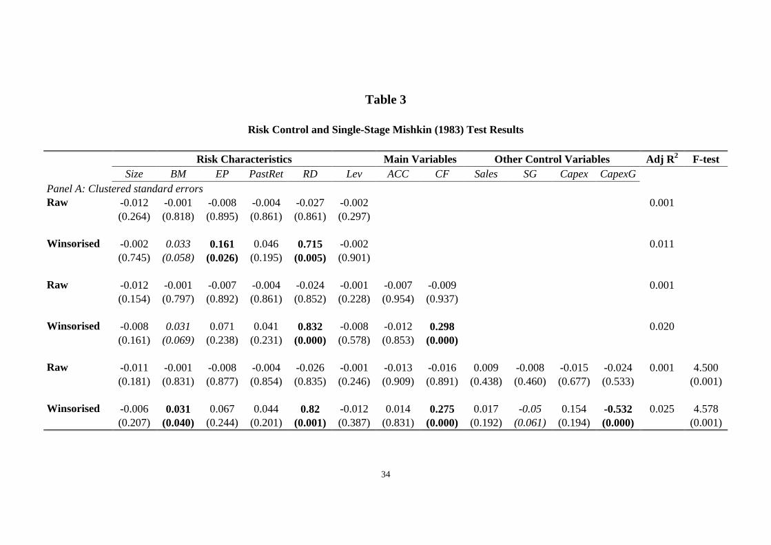
Table 3 provides the results of estimating equations (8) to (10). Panel A provides

estimates on both raw and winsorised data using OLS coefficients with time and firm

clustered standard errors. Panel B provides coefficient and standard error estimates

using the Fama and MacBeth (1973) approach. Coefficients that are significant at the

5% level, using a two-tailed test, are represented in bold type. Coefficients that are

significant at the 10% level, using a two-tailed test, are represented in italicised type.

Equations (9) and (10) represent Mishkin (1983) tests.

When dealing with raw data, the picture is straightforward. For the results using OLS

coefficients and time and firm clustered standard errors, there are no significant

coefficients, whether they be risk control variables, accruals or cash flow variables, or

additional forecasting variables. When using the Fama and MacBeth (1973) approach,

neither accruals nor cash flow have significant coefficients. Further, none of the

additional forecasting variables are significant. The ratio of research and development

expenditures is significant for all model specifications, with past returns becoming more

significant as the equation estimated moves from (8) to (10).

24

The picture is much changed when winsorised data are used. First, for the results using

OLS coefficients and time and firm clustered standard errors, some of the risk control

variables become significant. In particular, the ratio of research and development

expenditures is significant for all model specifications. The ratio of earnings to price

and the ratio of book to market are significant in particular specifications, with the

latter, whilst only significant at the 10% level for equations (8) and (9), significant at the

5% level for equation (10). One of the additional forecasting variables, capital

expenditure growth, has a significant and negative coefficient at the 5% level, with sales

growth having a negative coefficient which is significant at the 10% level. With respect

to the variables of interest, the accruals variable stays insignificant, but the cash flow

variable now has a significantly positive relationship with returns, whether it is equation

(9) or (10) being estimated.

When using the Fama and Macbeth (1973) approach, the picture is similar. More risk

control variables become significant (past returns and the earnings to price ratio become

consistently significant, along with leverage becoming significant at at least the 10%

level in all equations, with the book to market ratio ceasing to have significant

explanatory power). Sales growth loses significance, even at the 10% level. But, the

accruals variable still does not have a significant coefficient, and the cash flow

coefficient is significant and positive, whether it is equation (9) or (10) being estimated.

What the results in Table 3 do suggest is that, if winsorised data are employed, there is a

cash flow effect on annual returns. This result is robust to whether or not additional

earnings forecasting variables are included. This suggests that, if there is an effect

associated with earnings components on annual returns, it is due to the cash flow

25

component. Further, it is incremental to a general earnings effect captured by EP. As

pointed out earlier, however, it is not possible to conclude from these estimations if the

cash flow effect is caused by any mis-forecasting with respect to cash flows specifically.

Further, an alternative explanation is that the cash flow effect is caused by risk.

Overall, the results also contrast with those in Pincus et al. (2007), who find an accruals

effect but no cash flow effect on UK data when ignoring the effect of trading costs.

They use a number of methodologies. The first one involves a two-stage Mishkin test.

The second one involves a methodology similar to the one here, although with fewer

controls for risk. In particular, whilst they control for Size, BM and EP, they do not

include controls for RD, PastRet and Lev. The failure to control for these other firm

characteristics which do help explain returns to one extent or another in our sample

could account for the difference in results.

Finally, there is some evidence of the additional forecasting variables being mis-priced.

Nonetheless, the only consistently significant relationship, whichever estimation

approach is used, is a negative one for growth in capital expenditure when using

winsorised data.

To check the robustness of the results to alternative specifications of the accruals and

cash flow variables, we additionally estimate equations (12) and (13). In these

equations, we first substitute for ACC nine dummy variables corresponding to accruals

rank deciles two through ten in equation (9). Second, we substitute for CF nine dummy

variables corresponding to cash flow rank deciles two through ten. We maintain the

presence of the risk control variables and the other forecasting variables. The results are

26

shown in Table 4, with only the results for the accruals and cash flow variables being

reported. The results for the risk variables and additional forecasting variables have the

same qualitative characteristics as those reported in Table 3.

____________________________

Table 4

____________________________

When considering the impact of accruals decile rank dummies, if raw data are used, the

results are similar to those found in Soares and Stark (2009) for annual returns,

whichever estimation method is used. The coefficients of accruals rank deciles seven

(nine to ten) to ten are negative and are individually significant at a 5% level if OLS

coefficients and time and firm clustered standard errors (the Fama and MacBeth, 1973,

approach) are used. The coefficient of accruals decile rank six (seven and eight) is

negative and significant at the 10% level. The coefficient of cash flow is negative and

significant if OLS coefficients and time and firm clustered standard errors are used,

whereas it is negative and insignificant if the Fama and MacBeth (1973) approach is

employed.

If winsorised data are used, however, none of the accruals decile rank dummies are

significant, whichever estimation approach is employed.9 Further, as in Table 3, a

significantly positive coefficient for cash flow is estimated, again whichever estimation

approach is adopted.

9 An F-test suggests that the accruals decile rank dummies do jointly and significantly add

explanatory power, however.

27

When cash flow decile rank dummies are used, a significant, but positive, coefficient for

the accruals variable is observed when using raw data, but this result is not consistent

across estimation approaches. When winsorised data are used, neither estimation

approach produces a significant coefficient for the accruals variable. For both sets of

data, there is a generally positive, if not monotonic, trend in the coefficients of the cash

flow decile dummies as the cash flow decile ranks move from low to high. For both

sets of data, however, none of the cash flow decile dummy coefficients are significant

when OLS coefficients and time and firm clustered standard errors are employed.

When, the Fama and MacBeth (1973) approach is used, there are no significant

coefficients when raw data are used, but cash flow decile rank dummies six through ten

are positive and significant at the 5% level when winsorised data are used.10

Overall, there is little evidence for an accruals mis-pricing effect in which returns

decline as accruals increase, once an extended set of risk controls are taken into account.

In fact, there is stronger evidence suggesting that, in fact, there is a cash flow effect in

annual returns, even after risk controls have been taken into account. As indicated

above, however, an alternative interpretation is that the accruals effect is not a separate

effect, once the effects of other variables considered to predict future returns and/or

future earnings are taken into account, whereas the cash flow effect is separate.

10 When raw data are used, note that the coefficient of the cash flow decile rank two dummy is

negative and fairly large, suggesting that the average returns for that decile are lower than those for the lowest decile. This effect largely disappears when winsorised data are employed.

28

5 CONCLUSIONS

In this paper, we apply a modified one-stage version of the Mishkin (1983) test to

companies in the UK stock market in order to investigate the presence or otherwise of

the accruals anomaly in UK firms’ annual returns. We apply the test using an expanded

set of risk controls, relative to prior research, that have been found to have the ability to

predict returns in the UK.

For the period of 1990-2007, we report that there is little evidence of a general accruals

anomaly in the UK, in which accruals have a negative relationship with future returns,

once risk and other potential forecasting variables have been accounted for. We also

provide evidence that, after winsorising extreme observations, there is a cash flow

anomaly in the UK stock market. We also find evidence in favour of an anomaly with

respect to capital expenditure growth. Another interpretation is that the accruals

anomaly is not distinct from other anomalies in the UK market, whereas the cash flow

(and the capital expenditure growth) anomaly is.

Whether the cash flow and capital expenditure growth effects on returns are evidence of

actual anomalies is an interesting issue. One further possibility is that they capture

elements of risk not captured by the risk controls employed. .If such an explanation is

accepted, our results can be interpreted as suggesting the possibility of, for example, a

conditional capital asset pricing model, in which quite a number of firm characteristics

act as conditioning variables. Should this be the case, it suggests that empirical asset

pricing models need to be fairly complex to capture the effects of conditioning variables

29

in generating estimates of abnormal returns in the UK (and, possibly, elsewhere).

Investigating this possibility is a potentially interesting route for future research.

30

REFERENCES

Abel, A. B., and F. S. Mishkin, 1983. On the Econometric Testing of Rationality-Market Efficiency. Review of Economics & Statistics 65 (2), 318-323.

Al-Horani, A., P. F. Pope, and A. W. Stark, 2003. Research and Development Activity and Expected Returns in the United Kingdom. European Finance Review 7 (1), 161-181.

Chan, A. L. C., E. Lee, and S. Lin, 2009. The impact of accounting information quality on the mispricing of accruals: The case of FRS3 in the UK. Journal of Accounting and Public Policy 28 (3), 189-206.

Dedman, E., S. Mouselli, Y. U. N. Shen, and A. W. Stark, 2009. Accounting, Intangible Assets, Stock Market Activity, and Measurement and Disclosure Policy—Views From the U.K. Abacus 45 (3), 312-341.

Fama, E. F., and K. R. French, 1993. Common risk factors in the returns on stocks and bonds. Journal of Financial Economics 33 (1), 3-56.

Fama, E. F., and K. R. French, 1998. Value versus Growth: The International Evidence. Journal of Finance 53 (6), 1975-1999.

Fama, E. F., and J. D. MacBeth, 1973. Risk, Return, and Equilibrium: Empirical Tests. Journal of Political Economy 81 (3), 607-636.

Francis, J., and M. Smith, 2005. A reexamination of the persistence of accruals and cash flows. Journal of Accounting Research 43 (3), 413-451.

Gow, I. D., G. Ormazabal, and D. Taylor, 2010. Correcting for Cross-Sectional and Time-Series Dependence in Accounting Research. Accounting Review 85 (2), 483-512.

Gregory, A., R. D. F. Harris, and M. Michou, 2001. An Analysis of Contrarian Investment Strategies in the UK. Journal of Business Finance & Accounting 28 (9&10), 1192-1228.

Gregory, A., R. Tharyan, and A. C. Christidis, 2009. The Fama-French and Momentum Portfolios and Factors in the UK. SSRN eLibrary.

Kaserer, C., and C. Klinger, 2008. The Accrual Anomaly Under Different Accounting Standards – Lessons Learned from the German Experiment. Journal of Business Finance & Accounting 35 (7-8), 837-859.

Khan, M., 2008. Are accruals mispriced Evidence from tests of an Intertemporal Capital Asset Pricing Model. Journal of Accounting and Economics 45 (1), 55-77.

Kothari, S. P., J. S. Sabino, and T. Zach, 2005. Implications of survival and data trimming for tests of market efficiency. Journal of Accounting & Economics 39 (1), 129-161.

Kraft, A., A. J. Leone, and C. E. Wasley, 2006. An analysis of the theories and explanations offered for the mispricing of accruals and accrual components. Journal of Accounting Research 44 (2), 297-339.

31

Kraft, A., A. J. Leone, and C. E. Wasley, 2007. Regression-Based Tests of the Market Pricing of Accounting Numbers: The Mishkin Test and Ordinary Least Squares. Journal of Accounting Research 45 (5), 1081-1114.

LaFond, R., 2005. Is the Accrual Anomaly a Global Anomaly? , SSRN, http://ssrn.com/paper=782726

Leippold, M., and H. Lohre, 2008. Data Snooping and the Global Accrual Anomaly. SSRN, http://ssrn.com/paper=962867.

Liu, W., N. Strong, and X. Xu, 1999. The Profitability of Momentum Investing. Journal of Business Finance & Accounting 26 (9&10), 1043-1091.

Michou, M., S. Mouselli, and A. Stark, 2010. Fundamental Analysis and the Modelling of Normal Returns in the UK. SSRN, http://ssrn.com/paper=1607759.

Mishkin, F. S., 1983. A Rational Expectations Approach to Macroeconometrics: Testing Policy Ineffectiveness and Efficient-Markets Models. (Chicago, IL, University of Chicago Press for the National Bureau of Economics Research).

Petersen, M., 2009. Estimating Standard Errors in Finance Panel Data Sets: Comparing Approaches. Review of Financial Studies 22 (1), 435-480.

Pincus, M., S. Rajgopal, and M. Venkatachal, 2007. The Accrual Anomaly: International Evidence. Accounting Review 82 (1), 169-203.

Pope, P., 2001. Discussion of The Relation Between Incremental Subsidiary Earnings and Future Stock Returns in Japan. Journal of Business Finance & Accounting 28 (9-10), 1141-1148.

Sloan, R. G., 1996. Do Stock Prices Fully Reflect Information in Accruals and Cash Flows about Future Earnings? Accounting Review 71 (3), 289-315.

Soares, N., and A. W. Stark, 2009. The Accruals Anomaly - Can Implementable Portfolios Strategies be Developed that are Profitable in the UK? Accounting and Business Research 39 (4), 321-345.

Strong, N., and X. G. Xu, 1997. Explaining the Cross-Section of UK Expected Stock Returns. British Accounting Review 29 (1), 1-23.

32

Table 1

The Associations Between Ranking Firms By Accruals and the Independent Variables

AccDec ACC CF Ret Size BM EP PastRet RD Lev Sales SG Capex CapexG 1 -0.285 0.138 0.178 9.732 0.286 -0.237 0.071 0.033 0.694 1.847 0.435 0.121 0.045 2 -0.130 0.133 0.153 10.481 0.557 -0.037 0.100 0.025 0.713 1.465 0.108 0.099 0.021 3 -0.091 0.121 0.097 10.952 0.707 0.012 0.115 0.017 0.636 1.594 0.296 0.086 0.012 4 -0.066 0.119 0.123 11.277 0.649 0.053 0.105 0.017 0.839 1.397 0.118 0.095 0.025 5 -0.048 0.107 0.108 11.419 0.712 0.064 0.115 0.019 0.724 1.383 0.138 0.078 0.014 6 -0.032 0.091 0.108 11.475 0.640 0.082 0.118 0.015 0.546 1.295 0.144 0.074 -0.005 7 -0.015 0.072 0.074 11.183 0.836 -0.017 0.097 0.044 0.572 1.218 0.113 0.072 0.011 8 0.005 0.053 0.081 10.958 0.746 0.051 0.111 0.021 0.415 1.376 0.219 0.064 0.009 9 0.041 0.005 0.061 10.629 0.559 0.063 0.146 0.015 0.581 1.597 0.268 0.074 0.020 10 0.347 -0.338 0.042 10.269 0.340 0.044 0.203 0.014 0.450 3.039 1.549 0.114 0.062

Total -0.028 0.050 0.103 10.837 0.603 0.008 0.118 0.022 0.617 1.621 0.338 0.088 0.021

33

Table 2

Pearson (Lower Diagonal) and Spearman (Upper Diagonal) Correlations Between Independent Variables

ACC CF Ret Size BM EP PastRet RD Lev Sales SG Capex CapexG ACC -0.454 -0.041 0.061 0.015 0.145 0.047 -0.033 -0.053 0.062 0.209 -0.046 0.088 CF -0.993 0.150 0.323 -0.161 0.456 0.225 -0.030 -0.027 0.307 0.110 0.286 0.046 Ret 0.007 -0.009 0.079 0.067 0.154 0.102 0.009 0.023 0.052 -0.037 0.028 -0.047 Size -0.002 0.035 -0.031 -0.274 0.207 0.318 0.130 -0.053 0.007 0.128 0.262 0.120 BM -0.001 0.003 0.001 -0.046 0.235 -0.281 -0.093 0.314 -0.179 -0.220 -0.081 -0.102 EP 0.004 0.015 -0.001 0.101 -0.304 0.065 -0.091 0.321 0.298 0.115 0.184 0.016

PastRet 0.000 0.006 -0.009 0.152 -0.037 0.044 -0.033 -0.207 0.114 0.143 0.062 0.074 RD -0.001 -0.006 -0.003 -0.045 0.264 -0.928 -0.025 -0.093 -0.112 -0.074 -0.031 -0.021 Lev -0.001 0.000 -0.007 -0.072 -0.242 -0.106 -0.045 0.079 0.014 -0.126 0.027 -0.101

Sales 0.000 0.003 0.001 -0.004 -0.006 0.006 0.006 -0.003 -0.004 0.434 0.207 0.114 SG 0.001 0.001 0.000 0.001 -0.002 0.001 0.003 -0.001 -0.002 0.996 0.268 0.278

Capex -0.002 0.000 -0.022 0.011 -0.002 0.002 0.006 -0.005 -0.006 0.261 0.264 0.449 CapexG 0.000 -0.002 -0.022 0.005 -0.002 0.001 0.010 -0.002 -0.007 0.246 0.248 0.921

Notes: Bold type indicates significance at the 5% level or better.

34

Table 3

Risk Control and Single-Stage Mishkin (1983) Test Results

Risk Characteristics Main Variables Other Control Variables Adj R2 F-test Size BM EP PastRet RD Lev ACC CF Sales SG Capex CapexG

Panel A: Clustered standard errors -0.012 -0.001 -0.008 -0.004 -0.027 -0.002 0.001 Raw (0.264) (0.818) (0.895) (0.861) (0.861) (0.297)

-0.002 0.033 0.161 0.046 0.715 -0.002 0.011 Winsorised (0.745) (0.058) (0.026) (0.195) (0.005) (0.901)

-0.012 -0.001 -0.007 -0.004 -0.024 -0.001 -0.007 -0.009 0.001 Raw (0.154) (0.797) (0.892) (0.861) (0.852) (0.228) (0.954) (0.937)

-0.008 0.031 0.071 0.041 0.832 -0.008 -0.012 0.298 0.020 Winsorised (0.161) (0.069) (0.238) (0.231) (0.000) (0.578) (0.853) (0.000)

-0.011 -0.001 -0.008 -0.004 -0.026 -0.001 -0.013 -0.016 0.009 -0.008 -0.015 -0.024 0.001 4.500 Raw (0.181) (0.831) (0.877) (0.854) (0.835) (0.246) (0.909) (0.891) (0.438) (0.460) (0.677) (0.533) (0.001)

-0.006 0.031 0.067 0.044 0.82 -0.012 0.014 0.275 0.017 -0.05 0.154 -0.532 0.025 4.578 Winsorised (0.207) (0.040) (0.244) (0.201) (0.001) (0.387) (0.831) (0.000) (0.192) (0.061) (0.194) (0.000) (0.001)

35

Table 3 (cont'd)

Risk Control and Single-Stage Mishkin (1983) Test Results

Risk Characteristics Main Variables Other Control Variables Adj R2 F-test Size BM EP PastRet RD Lev ACC CF Sales SG Capex CapexG

Panel B: Fama-MacBeth -0.013 -0.017 0.023 0.043 0.536 -0.002 0.039 Raw (0.213) (0.503) (0.696) (0.115) (0.009) (0.829)

-0.004 0.021 0.125 0.069 0.790 -0.019 0.048 Winsorised (0.536) (0.124) (0.007) (0.013) (0.004) (0.096)

-0.010 -0.013 0.043 0.050 0.498 -0.001 -0.143 -0.084 0.052 Raw (0.199) (0.542) (0.282) (0.066) (0.009) (0.869) (0.160) (0.589)

-0.006 0.019 0.095 0.067 0.819 -0.022 -0.061 0.151 0.058 Winsorised (0.246) (0.170) (0.012) (0.017) (0.002) (0.045) (0.418) (0.019)

-0.009 -0.012 0.042 0.054 0.500 -0.002 -0.150 -0.091 0.004 -0.002 0.027 -0.230 0.059 1.187 Raw (0.215) (0.562) (0.304) (0.048) (0.010) (0.845) (0.154) (0.567) (0.595) (0.763) (0.816) (0.106) (0.352)

-0.005 0.020 0.091 0.066 0.797 -0.025 -0.058 0.143 0.008 -0.022 -0.007 -0.29 0.068 4.923 Winsorised (0.326) (0.130) (0.014) (0.017) (0.003) (0.023) (0.492) (0.024) (0.366) (0.152) (0.930) (0.002) (0.008)

Notes: p-values in parenthesis. Bold type indicates significance at the 5% level or better. Italicised type indicates significance at the 10% level but not the 5% level. The F-test results are for whether the ‘Other Control Variables’ significantly add to explanatory power.

36

Table 4

Cash Flow and Accruals Decile Effects on Annual Returns

ACCDEC2 ACCDEC3 ACCDEC4 ACCDEC5 ACCDEC6 ACCDEC7 ACCDEC8 ACCDEC9 ACCDEC10 CF Adj R2

Panel A: Clustered standard errors -0.016 -0.066 -0.036 -0.049 -0.049 -0.085 -0.082 -0.107 -0.131 -0.004 0.003 Raw (0.509) (0.052) (0.252) (0.134) (0.081) (0.044) (0.035) (0.002) (0.000) (0.006)

0.022 -0.003 0.024 0.018 0.019 0.002 0.006 0.000 0.016 0.274 0.025 Winsorised

(0.168) (0.868) (0.353) (0.469) (0.396) (0.950) (0.843) (0.987) (0.612) (0.000) Panel B: Fama-MacBeth

-0.015 -0.055 -0.027 -0.050 -0.041 -0.075 -0.081 -0.107 -0.146 -0.124 0.067 Raw (0.613) (0.112) (0.380) (0.195) (0.250) (0.096) (0.094) (0.042) (0.027) (0.433)

0.018 -0.007 0.015 -0.003 0.006 -0.015 -0.020 -0.028 -0.038 0.113 0.075 Winsorised

(0.264) (0.644) (0.452) (0.882) (0.731) (0.517) (0.476) (0.260) (0.163) (0.038)

37

Table 4 (cont'd)

Accruals and Cash Flow Decile Effects on Annual Returns

ACC CFDEC2 CFDEC3 CFDEC4 CFDEC5 CFDEC6 CFDEC7 CFDEC8 CFDEC9 CFDEC10 Adj R2

Panel C: Clustered standard errors 0.003 -0.072 -0.003 -0.015 -0.014 0.031 0.044 0.044 0.038 0.083 0.003 Raw

(0.000) (0.410) (0.964) (0.874) (0.879) (0.742) (0.629) (0.609) (0.652) (0.294)

-0.092 -0.008 0.030 0.017 0.015 0.048 0.064 0.058 0.055 0.092 0.021 Winsorised (0.363) (0.822) (0.509) (0.767) (0.779) (0.449) (0.318) (0.360) (0.395) (0.162)

Panel D: Fama-MacBeth

-0.038 -0.062 0.014 0.005 -0.002 0.035 0.042 0.036 0.032 0.065 0.063 Raw (0.511) (0.382) (0.793) (0.935) (0.977) (0.621) (0.552) (0.628) (0.643) (0.363)

-0.037 0.013 0.060 0.056 0.053 0.083 0.099 0.092 0.089 0.119 0.075 Winsorised (0.664) (0.646) (0.072) (0.133) (0.139) (0.044) (0.021) (0.038) (0.028) (0.005)

Notes: p-values in parenthesis. Bold type indicates significance at the 5% level or better. Italicised type indicates significance at the 10% level but not the 5% level.