Embed Size (px)
Citation preview

PROCEEDINGS
IConSSM 2011
The 3rd International Congress of Serbian Society of Mechanics
Vlasina lake (Serbia), 5-8 July 2011
Editors Stevan Maksimović
Tomislav Igić

The 3rd International Congress of Serbian Society of Mechanics (IConSSM 2011) Editors Stevan Maksimović Tomislav Igić Computer editing Marija Blažić, Ivana Ilić Press Klasa, Belgrade http://www.klasa.rs/ Circulation 250 copies CIP – Каталогизација у публикацији Народна библиотека Србије, Београд 531/534(082) СРПСКО друштво за механику (Београд). Међународни конгрес (3; 2011; Vlasinsko jezero) Proceedings/The 3rd International Congress of Serbian Society of Mechanics (IConSSM 2011), Vlasina lake (Serbia), 5-8 July 2011; editors Stevan Maksimović, Tomislav Igić. – Beograd: Serbian Society of Mechanics; 2011 (Belgrade: Klasa).- VII, 1244 str.: ilustr.; 25 cm Tiraž 250. – Str.III: Preface/Stevan Maksimović, Tomislav Igić.,- Bibliografija uz svaki rad. ISBN 978-86-909973-3-6 a) Механика - Зборници COBISS:SR-ID 187662860
Published by Serbian Society of Mechanics, Belgrade
http://www.ssm.org.rs/

PREFACE The proceedings contains the papers presented at the Third (28th Yu) International Congress of Serbian Society of Mechanics held in Vlasina lake during the period 5th -8th July, 2011. Theoretical and Applied Mechanics is a subject of great importance in the developing of science and technology. The aim of the Congress is to provide a forum to exhibit the progress in this field during the past two years and a place to further the interaction of modern theoretical and applied mechanics, as well as modern engineering sciences. The papers, contributed by authors from all around the globe, have been separated into 7 sections which cover the main areas of the interest, e. g. `Plenary lectures`, Section A, Section B, Section C, Section D and two Mini-symposia. We would here like to express our heartfelt thanks to all members of the Scientific Committee and also to the participants for their engagement in organizing of the Congress, including the preparation of manuscripts which will be published in the Journal Theoretical and Applied Mechanics and Scientific Technical Review. Last, but by no means least, the Congress organizing committee wishes to acknowledge the collaboration of the Ministry of Education and Science – Government of the Republic of Serbia, Municipatily Surdulica and Many Supporting members of the Serbian Society of Mechanics listed in the proceedings.
Stevan Maksimović & Tomislav Igić
Chairmen of Organizing Committee July, 2011.

The 3rd International Congress of Serbian Society of Mechanics IConSSM 2011, Vlasina lake (Serbia), 5-8 July 2011. Scientific Committee Nikola Hajdin (Belgrade, Serbia) Vladan Đorđević (Belgrade, Serbia), Božidar Vujanović (Novi Sad, Serbia) Đorđe Zloković (Belgrade, Serbia) Felix Chernousko (Moscow, Russia) Antony Kounadis (Athens, Greece) Ingo Müller (Berlin, Germany) Đorđe Đukić (Novi Sad, Serbia) Teodor Atanacković (Novi Sad, Serbia) Miloš Kojić (Kragujevac, Serbia) Ranislav Bulatović (Podgorica, Montenegro) Katica (Stevanović) Hedrih (Belgrade, Serbia) Anatoly M. Samoilenko (Kiev, Ukraine) Emanuel Gdoutos (Thrace, Greece) Hiroshi Yabuno (Tokiyo, Japan) John Katsikadelis (Athens, Greece) M. P. Cartmell (Glasgow, Scotland, UK) Giuseppe Rega (Roma, Italy) Jan Awrejcewicz (Lodz, Poland) Jmbal Thazar (Sao Paolo, Brazil) Robin Tucker (Lancaster, England) Gerard Maugin (Paris, France) J. A. Tenreiro Machado (Porto, Portugal) Dumitru Baleanu (Ankara, Turkey) Subhash C. Sinha (Auburn, Alabama) Jerzy Warminski (Lublin, Poland) Yuri Mikhilin (Kharkov, Ukraine) Radu Miron (Iashi, Romania) Joseph Zarka (Palaiseau, France) Alexander Seyranin (Moscow, Russia) Chi Chow (Michigen, United States) Lidia Kurpa (Khrakov, Ukraine) Jovo Jarić (Belgrade, Serbia)
Mihajlo Lazarević (Belgrade, Serbia) Reinhold Kienzler (Bremen, Germany) Rade Vignjević (Grenfield, England) Andrea Carpinteri (Parma, Italy) Miloš Nedeljković (Belgrade, Serbia) Milorad Milovancević (Belgrade ,Serbia) Tamara Nestorović (Bohum, Germny) Guy Guerlement (Mons, Belgium) Atual Bhaskar (Southampton, England) Bohdana Marvalova (Chesc Republic) Jorge Ambrosio (Lisabon, Portugal) Pedro Ribeiro (Porto, Portugal) Livija Cvetičanin (Novi Sad, Serbia) Milan Mićunović (Kragujevac, Serbia) Dragan Milosavljević (Kragujevac, Serbia) Vladimir Dragović (Belgrade, Serbia) Vladimir Raičević (Kosovska Mitrovica, Serbia) Zlatibor Vasić (Kosovska Mitrovica, Serbia) Vladimir Stevanović (Belgrade, Serbia) Zoran Mitrović (Belgrade, Serbia) Predrag Kozić (Niš, Serbia) Ratko Pavlović (Niš, Serbia) Dragoslav Kuzmanović (Belgrade, Serbia) Dragoslav Šumarac (Belgrade, Serbia) Dragan Aranđelović (Niš, Serbia) Vlastimir Nikolić (Niš, Sebia) Taško Maneski (Belgrade, Serbia) Nataša Trišović (Belgrade, Serbia) Borislav Gajić (Belgrade, Serbia) Srboljub Simić (Novi Sad, Serbia) Dragan Spasić (Novi Sad, Serbia) Tomislav Igić (Nis, Serbia) Stevan Maksimović (Belgrade, Serbia)
Organizing Committee Stevan Maksimović (co-chairman) Tomislav Igić (co-chairman) Borislav Gajić, sekretary Slobodanka Boljanović Nataša Trišović Ivana Vasović Dragi Stamenković Ivana Ilić Marija Blažić

TABLE OF CONTENTS
PREFACE No. PLENARY LECTURES P-01 E.E. Gdoutos
FAILURE OF SANDWICH STRUCTURES 2
P-02 R. Vignjević, J. Campbell BRIEF REVIEW OF DEVELOPMENT OF THE SMOOTH PARTICLE HYDRODYNAMICS (SPH) METHOD
24 P-03
M. Lazarević STABILITY OF FRACTIONAL ORDER TIME DELAY SYSTEMS
44
P-04 A. P. Seyranian INTERACTION OF EIGENVALUES WITH APPLICATIONS IN MECHANICS AND PHYSICS
70 P-05 M. Živković, G. Jovičić
NUMERICAL METHODS IN FRACTURE MECHANICS 80 P-06 S. C. Sinha, A. Gabale
REDUCED ORDER MODELS FOR ANALYSIS AND CONTROL OF NONLINEAR SYSTEMS WITH PERIODIC COEFFICIENTS
94 LIST OF PAPERS Section A - GENERAL MECHANICS
A-03 V. Dragović, K. Kukić DISCRIMINANT SEPARABILITY AND KOWALEVSKI-TYPE SYSTEMS
96
A-04 Y. N. Fedorov, B. Jovanović INTEGRABLE SYSTEMS ON STIEFEL VARIETIES
114
A-05
M. P. Lazarević, Lj. Bučanović FURTHER RESULTS ON PID TYPE CONTROL OF EXPANSION TURBINE IN THE AIR PRODUCTION CRYOGENIC LIQUID
122 A-06 S. Mastilović
SOME NOTES ON STOCHASTICITY OF DYNAMIC RESPONSE OF 2D BRITTLE LATTICES
137 A-07 M. Mićunović, Lj. Kudrjavceva
ON VISCOPLASTICITY OF TRANSVERSELY ISOTROPIC QUASI-RATE INDEPENDENT MATERIALS
149 A-08 Z. Mitrović, S. Rusov, N. Mladenović, A. Obradović
FUZZY OPTIMIZATION OF CANTILEVER BEAM 158
A-09 D. Perišić STOCHASTIC MINIMAX DYNAMIC GAMES WITH INFORMATION CONSTRAINTS
154 A-10 D. Perišić
STOCHASTIC OPTIMAL CONTROL WITH JUMPS AND INFORMATION CONSTRAINTS
171 A-11 D. Radojević
A NOTE ON KASNER METRIC 177
A-15 V. Vujičić MOND TEORIJA MODIFIKACIJA NJUTNOVSKE DINAMIKE
179
A-16 N. Zorić, Z. Mitrović, A. Simonović MULTI-OBJECTIVE OPTIMIZATION OF PIEZOELECTRIC SENSOR AND ACTUATOR PLACEMENT AND SIZING FOR ACTIVE VIBRATION CONTROL
194
i

A-18 M. Živanović CONTROL FORCE FOR SCLERONOMIC MECHANICAL SYSTEM IN DECOMPOSITION MODE
209
Section B - FLUID MECHANICS B-01 J. Bogdanović-Jovanović, Ž. Stamenković
INFLUENCE OF DUCT CROSS-SECTION ON THE FLOW CHARACTERISTICS AROUND A SMOOTH SPHERE
222 B-02 Z. Boričić, D. Nikodijević, Z. Stamenković
UNSTEADY TEMPERATURE MHD BOUNDARY LAYER ON THE POROUS BODY OF ARBITRARY SHAPE
236 B-03 Đ. Čantrak, M. Nedeljković, N. Janković
TURBULENT SWIRL FLOW DYNAMICS
251 B-05 D. Jerković, S. Ilić, A. Kari, D. Regodić
THE RESEARCH ON THE AERODYNAMIC COEFFICIENT EFFECTS ON THE STABILITY OF THE CLASSIC AXIS-SYMMETRICAL PROJECTILE
262 B-07 M. Jovanović, J. Nikodijević
NUMERICAL SIMULATION OF PERTURBED POISEUILLE-COUETTE FLOW
275 B-08 M. Kozić, S. Ristić, M. Puharić, B. Katavić
COMPARISON OF EULER-EULER AND EULER-LAGRANGE APPROACH IN NUMERICAL SIMULATION OF MULTIPHASE FLOW IN VENTILATION MILL
290 B-09 S. Linić, M. Puharić, D. Matić, V. Lučanin
DETERMINATION OF THE AERODYNAMIC BRAKES FOR VARIOUS HIGH SPEED TRAIN VELOCITIES
304 B-11 N. Mirkov, N. Vidanović, B. Rašuo
NUMERICAL SIMULATION OF SEPARATED TURBULENT FLOW IN ASYMMETRIC DIFFUSERS
312 B-12 B. Stanković, S. Belošević, M. Sijerčić, N. Crnomarković, V. Beljanski,
I.Tomanović, A. Stojanović INVESTIGATION OF FULLY DEVELOPED PLANE TURBULENT CHANNEL FLOW BY MEANS OF REYNOLDS STRESS MODELS
321 Section C - MECHANICS OF SOLID BODIES
C-01 N. Anđelić, V. Milošević-Mitić, T. Maneski THIN-WALLED OPEN-SECTION BEAMS – ONE VIEW TO THE OPTIMIZATION ACCORDING TO STRESS CONSTRAINTS
340 C-02 I. Atanasovska
THE INFLUENCE OF LOAD AND BOUNDARY CONDITION SIMULATION ON THE STRUCTURAL EVALUATION OF RAILWAY WAGONS WITH FINITE ELEMENT TOOLS
352 C-03 A. Bhaskar
TRAPPED WAVES AND END EFFECTS IN ELASTIC WAVEGUIDES
366 C-05 M. Blažić, K. Maksimović, Y. Assoul
DETERMINATION OF STRESS INTENSITY FACTORS OF STRUCTURAL ELEMENTS BY SURFACE CRACKS
374 C-06 M. Bojanić
STABILITY ANALYSIS OF LAYERED COMPOSITE PANELS BY FINITE ELEMENTS
384 C-07 S. Boljanović, S. Maksimović, A. Carpinteri
ii

NUMERICAL MODELING OF SEMI-ELLIPTICAL CRACK GROWTH UNDER CYCLIC LOADING
391
C-08 I. Čamagić, N. Vasić, Z. Burzić, P. Živković, Z. Vasić
APPLICATION OF FRACTURE MECHANICS PARAMETERS FOR WELDED JOINTS USABILITY TESTING
399 C-09 M. Ćetković, Đ. Vuksanović
GEOMETRICALLY NONLINEAR ANALYSIS OF LAMINATE COMPOSITE PLATES
411 C-11 J. Dautović, S. Đurković, V. Madić
ONE METHOD OF NON-CONTACT SHAFT TORQUE MEASUREMENT 425
C-12 J. Đoković THE BEHAVIOR OF THE INTERFACIAL CRACK BETWEEN THE TWO LAYERS UNDER CONDITIONS OF A STATIONARY TEMPERATURE FIELD
440 C-13 E. Džindo, A. Sedmak, B. Petrovski
ELASTO-PLASTIC FRACTURE MECHANICS FINITE ELEMENT ANALYSIS 448
C-14 P. Elek, V. Džingalašević, S. Jaramaz DETERMINATION OF DETONATION PRODUCTS EQUATION OF STATE USING CYLINDER TEST
457 C-15
V. Golubović-Bugarski, D. Blagojević, J. Škundrić
METHODS OF VERIFYING THE FREQUENCY RESPONSE FUNCTIONS QUALITY IN MODAL TESTING
471 C-16
A. Grbović, N. Vidanović, K. Čolić, D. Jevremović
THE USE OF FINITE ELEMENT METHOD (FEM) FOR ANALYZING STRESS DISTRIBUTION IN ADHESIVE INLAY BRIDGES
481 C-17 A. Grbović, N. Vidanović, G. Kastratović
THE USE OF FINITE ELEMENT METHOD (FEM) FOR SIMULATING CRACK GROWTH IN MINI DENTAL IMPLANTS (MDI)
490 C-18 I. Grozdanović
NOISE INDUCED COHERENT OSCILATIONS IN FITZ HUGH-NAGUMO EXCITABLE SYSTEMS INFLUENCED BY COUPLING DELAY
502 C-19 T. Igić, D. Turnić
OPTIMUM GIRDER DESIGN WITH MULTIPLE FUNCTIONS 509
C-21 G. Janevski, P. Kozić, I. Pavlović MOMENT LYAPUNOV EXPONENTS AND STOCHASTIC STABILITY OF A THIN-WALLED BEAM DRIVEN BY REAL NOISE
517 C-22 J.Jarić, R.Vignjević, Z. Golubović, D. Kuzmanović
ON ENTROPY FLUX OF ANISOTROPIC ELASTIC BODIES
534 C-23 D. Jevtić, D. Zakić, A. Savić, A. Radević
PROPERTIES OF COMPOSITE MATERIALS MADE WITH THE ADDITION OF RECYCLED RUBBER
547 C-26 S. Kostić, B. Deretić-Stojanović, S. Stošić
EFFECT OF CREEP AND SHRINKAGE ANALYSIS ON DEFLECTIONS OF CONTINUOUS COMPOSITE BEAMS
557 C-27 M. Kutin, S. Ristić, M. Puharić, M. Ristić
TENSILE FEATURES OF CONTRACTUAL HOLE IN PLATE SPECIMEN TESTING BY THERMOGRAPHY AND CONVENTIONAL METHOD
563
C-28 V. Kvrgić, J. Vidaković, V. Kaplarević, M. Lazarević FORWARD AND INVERSE KINEMATICS FOR VERTICAL 5-AXIS TURNING CENTER WITH ANGULAR HEAD OF NON-INTERECTIONAL AXES, WITH COMPENSATION FOR TABLE MOVING CAUSED BY THERMAL DILATATION
574 C-29 A. A. Liolios, C. E. Chalioris, K. A. Liolios
A NUMERICAL APPROACH FOR REINFORCED CONCRETE
iii
STRUCTURES ENVIRONMENTALLY DAMAGED AND CABLE-STRENGTHENED
590
C-30 J. Lozanović-Šajić STRUCTURAL INTEGRITY AND LIFE WITH STEREOMETRIC MACHINE VISION
598 C-31 S. Maksimović, I. Vasović, M. Maksimović, M. Đurić
RESIDUAL LIFE ESTIMATION OF DAMAGED STRUCTURAL COMPONENTS USING LOW-CYCLE FATIGUE PROPERTIES
605 C-32 R. Mandić, R. Salatić, Z. Perović
NUMERICAL MODELLING OF MASONRY WALLS SUBJECTED TO LATERAL IN-PLANE LOAD
618 C-33 T. Maneski, P. Jovančić, D. Ignjatović, V. Milošević-Mitić, N. Trišović
NUMERICAL AND EXPERIMENTAL DIAGNOSTIC OF DYNAMIC BEHAVIOR OF THE ROTOR-EXCAVATOR CONSTRUCTION
629 C-34 Lj. Marković, D. Ružič, H. Hertha-Haverkamp, C. Kardelky
SOME APPLICATIONS AND CONSTRAINTS OF THE FEM WITHIN THE MODAL ANALYSIS OF THE STRUCTURES
637 C-35 B. Medjo, M. Rakin, M. Arsić, Ž. Šarkoćević, A. Sedmak
MICROMECHANICAL APPROACH TO INTEGRITY ASSESSMENT OF SURFACE DAMAGED PIPES
645 C-36 R. Mijailović
DETERMINATION OF OPTIMUM DIMENSION OF VARIABLE SHAPE LATTICE-COLUMNS FOR BUCKLING
655 C-37 R. Mijailović
MATHEMATICAL MODELING OF FUNCTIONS DEPENDENCE OF FORCE – DEFORMATION IN A COLLISION OF VEHICLES
668 C-39 V. Milošević-Mitić, T. Maneski, N. Anđelić
BENDING OF A THIN PLATE SUBJECTED TO STRONG UNIFORM MAGNETIC FIELD
676 C-40 G. Milovanović , T. Igić, N. Tončev
SOME QUADRATURE RULES FOR FINITE ELEMENT METHOD AND BOUNDARY ELEMENT METHOD
684 C-41 S. Mitić
CRITERIA OF ELASTIC STABILITY FOR PLATE WITH GEOMETRIC DISCONTINUITY
693 C-43 M. Ognjanović, M. Benur
VIBRATIONS AS DESIGN CONSTRAINT IN MACHINE SYSTEMS DESIGN 707
C-44 M. Perić, D. Stamenković, V. Milković AN ENGINEERING APPROACH TO WELDING SIMULATION USING SIMPLIFIED MATERIAL PROPERTIES
715 C-45 S. Posavljak, M. Janković , K. Maksimović
DAMAGE OF AERO ENGINE DISKS IN FUNCTION OF CYCLYC MATERIAL PROPERTIES AND TYPE OF ENGINE START-STOP CYCLES
723 C-48 D. Rakić, M. Živković
STRESS INTEGRATION OF THE MOHR-COULOMB MATERIAL MODEL USING INCREMENTAL PLASTICITY THEORY
734 C-49 D. Ristić, J. Kramberger
NUMERICAL DETERMINATION OF CRITICAL STRESSES AND CRACK GROWTH IN A SPUR GEAR TOOTH ROOT
744 C-51 R. Slavković, V. Slavković, M. Živković, V. Dunić
STRESS INTEGRATION FOR FCC CRYSTAL PLASTICITY BY FINITE ELEMENT METHOD
757 C-52 V. Stojanović, P. Kozić, D. Jovanović
iv

BUCKLING OF ELASTICALLY CONNECTED TIMOSHENKO BEAMS UNDER COMPRESSIVE AXIAL LOADING
767
C-53 D. Šumarac, J. Dragaš LIMIT ANALYSIS OF PLATES
779
C-54 D. Šumarac, S. Jocković, M. Marjanović STATIC AND KINEMATIC HEIGHT LIMIT OF VERTICAL SLOPE
790
C-55 Mirjana Tomičić-Torlakovi, Vidan Rađen SLAB TRACK WITH "MASS-SPRING" SYSTEM
807
C-56 N. Trišović, T. Maneski, Lj. Milović, T. Lazović REANALYSIS FOR STRUCTURAL DYNAMIC MODIFICATIONS
816
C-57 N. Vasić, I. Čamagić, Z. Vasić HIGH TEMPERATURE INFLUENCE ON SANDWICH BEAM STABILITY
824
C-58
N. Vidanović, G. Kastratović, A. Grbović THE ANALYSIS OF CONTACT EFFECTS IN WIRE ROPE STRAND USING THE FINITE ELEMENT METHOD
836 C-59 S. Zdravković, T. Igić, D. Turnić
REQUIRED MECHANICAL PROPERTIES OF THE MATERIAL DURING CALCULATION OF MASONRY BUILDINGS IN SEISMIC AREAS
846
C-60 D. Zlatkov, S. Zdravković, T. Igić, B. Mladenović DESIGN OF SYSTEMS WITH SEMI-RIGID CONNECTIONS BY DEFORMATION METHOD ACCORDING TO THE SECOND-ORDER THEORY
858 C-63 M. Žigić, N. Grahovac
DYNAMICAL BEHAVIOR OF A POLYMER GEL DURING IMPACT FRACTIONAL DERIVATIVE VISCOELASTIC MODEL
871 C-64 M. Živković, A. Dišić
HOPKINSON BAR AS MOST USEFULLY TECHNIQUE IN MATERIAL TESTING AT HIGH STRAIN RATE
879 C-65 M. Živković, M. Topalović, R. Slavković, V. Dunić
ABAQUS SUBROUTINE DEVELOPMENT AND IMPLEMENTATION FOR NEO-HOOK HYPERELASTIC MATHERIAL MODEL
889 C-66 Ivana Ilić, Mirjana Đurić
NUMERICAL SIMULATION OF MECHANICALLY FASTENED JOINTS BY FINITE ELEMENTS
897
Section D - INTERDISCIPLINARY AND MULTIDUISCIPLINARY PROBLEMS
D-01 M. Blagojević, M. Živković,R. Slavkovic ELECTROSTATIC FIELD ANALYSIS USING HEAT TRANSFER ANALOGY
910
D-02 Z. Gajić, S. Mandić, M. Milošević, S. Stojković DETERMINATION OF MINIMAL ROLL RATE OF GYRO-STABILIZED ROCKET
920 D-03
S. Mandić, V. Vukmirica, S. Stojković GUIDED EARTH TO EARTH MISSILE IMPACT POINT DISPERSION DUE TO COMMERCIAL MEASUREMENT ERRORS
930 D-04 M. Milošević, D. Živanić, V. Đurković
THE OPTIMIZATION OF LAUNCHING CADENCES FROM SELF-PROPELLED MULTIPLE LAUNCHERS
942 D-05 M. Nefovska-Danilović, M. Petronijević, M. Radišić
ANALYSIS OF TRAFFIC INDUCED BUILDING VIBRATIONS USING SPECTRAL ELEMENT METHOD
956 D-06 R. Pavlović, I. Pavlović, V. Stojanović
v

INFLUENCE OF TRANSVERSE SHEAR AND ROTARY INERTIA ON VIBRATION AND STABILITY OF CROSS-PLY LAMINATED PLATES
975
D-08
S. Petronić, A. Milosavljević, A. Kovačević, B. Grujić, K. Čolić LASER SHOCK PEENING OF DEFORMED N-155 SUPERALLOY
986
D-09 M. Radišić, M. Nefovska-Danilović, M. Petronijević APPLICATION OF INTEGRAL TRANSFORM METHOD TO CALCULATE IMPEDANCE FUNCTIONS
994 D-10 A. Rinaldi, S. Mastilović
CONSTITUTIVE RELATIONS FOR HARDENING AND SOFTENING OF BRITTLE 2D LATTICES
1007 D-13 M. Šelmić, R. Šelmić
PACKAGE TRANSPORT USING GRAVITY CHUTE SYSTEM - FUZZY LOGIC APPROACH
1022 D-15 D. Živanić, V. Đurković, S. Jovančić
ANALYZING METHODS FOR THE RESPONSES OF THE LAUNCHING SYSTEM SUBJECTED TO THE STOCHASTIC EXCITATION CAUSED BY WIND
1038
Mini-symposium M1 – COMPUTATIONAL BIOMECHANICS M1-01 V. Isailović, T. Djukić, M. Ferrari, N. Filipović, M. Kojić
MOTION OF CIRCULAR AND ELLIPTICAL PARTICLES IN LAMINAR FLOWS
1049 M1-02 D. Milašinović, A. Cvetković, N. Filipović, M. Kojić
SIMULATION OF THE CONDITIONS LEADING TO DUODENAL STUMP DISRUPTION AFTER BILLROTH II GASTRIC RESECTION
1059 M1-03 M. Milošević, A. Ziemus, M. Ferrari, M. Kojić
MODELING OF DIFFUSION WITHIN NANOCHANNELS WITH SURFACE EFFECTS
1073
M1-04 Z. Milošević, B. Stojanović, V. Isailović, D. Nikolić, D. Milašinović, M. Radović, T. Exarchos, K. Stefanou, P. Siogkas, A. Sakelarios, D. Fotiadis, O. Parodi, N.Zdravković, M. Kojić, N. Filipović ARTOOL: A PLATFORM FOR THE DEVELOPMENT OF MULTI-LEVEL PATIENT-SPECIFIC ARTERY AND ATHEROGENESIS MODELS
1082 M1-05 M. Obradović, A. Avilla, A. Thiagalingam, N. Filipović
MODELING ABLATION ON THE ENDOCARDIUM AND TEMPERATURE DISTRIBUTION DURING RF ABLATION
1089 M1-06 D. Petrović, M. Obradović, A. Jovanović, S. Jovanović, D. Balos, M. Kojić,
N.Filipović DPD MODELING OF INHIBITION PROCESS OF COROSION PROTECTION USING NANOCONTAINERS
1104
M1-07 M. Radović, D. Petrović, N. Filipović DATA MININIG APPLICATION IN THE WALL SHEAR STRESS DISTRIBUTION PREDICTION FOR ANEURYSM AND CAROTID BIFURCATION MODELS
1112 Mini-symposium M2 – NONLINEAR DYNAMICS
M2-02 R. M. Bulatović, M. Kažić ON THE DEGREE OF INSTABILITY OF MECHANICAL SYSTEMS
1122
M2-03 L. Cvetićanin REVIEW ON MECHANICAL MODELING OF THE HUMAN VOICE PRODUCTION SYSTEMS
1131
M2-04 C. Frigioiu
vi

vii
GEOMETRIC ASPECTS OF NONHOLONOMIC MECHANICAL SYSTEMS 1139 M2-06 A. Hedrih, K. Stevanović-Hedrih
MODELING DOUBLE DNA HELIX MAIN CHAINS FORCED VIBRATIONS 1147
M2-07 K. Stevanović-Hedrih TANGENT SPACES OF POSITION VECTORS AND ANGULAR VELOCITIES OF THEIR BASIC VECTORS IN DIFFERENT COORDINATE SYSTEMS
1181 M2-09 K. Stevanović-Hedrih, Lj. Veljović
ANALYSIS OF THE VECTOR ROTATORS OF A RIGID BODY NONLINEAR DYNAMICS ABOUT TWO AXES WITHOUT SECTION
1194 M2-10 S. Jović, V. Raičević
ENERGY ANALYSIS OF VIBRO-IMPACT SYSTEM BASED ON OSCILLATOR MOVING FREELY ALONG CURVILINEAR ROUTES AND NON-LINEAL RELATIONS
1202 M2-11 J. T. Katsikadelis
A NEW DIRECT TIME INTEGRATION METHOD FOR THE EQUATIONS OF MOTION IN STRUCTURAL DYNAMICS
1222 M2-15 A. Obradović, S. Šalinić, O. Jeremić, Z. Mitrović
BRACHISTOCHRONIC MOTION OF A VARIABLE MASS SYSTEM 1237 M2-16 V. Raičević, S. Jović
VIBRO-IMPACT SYSTEM BASED ON OSCILLATOR, WITH TWO HEAVY MASS PARTICLES MOVING ALONG A ROUGH PARABOLA 1247
M2-20 Vera Nikolić-Stanojević, Ćemal Dolićanin, Ljiljana Veljović, Milica Obradović DYNAMIC MODELS OF BUILDINGS TO MITIGATE FLUCTUATIONS 1259
M2-21 A.Ćoćić, I.Guranov, M.Lečić NUMERICAL INVERTIGATION OF LAMINAR FLOW IN SQUARE CURVED DUCT WITH 90O BEND 1275
M2-22 Z. Rakarić, I. Kovačić
DETERMINATION OF STRESS INTENSITY FACTORS OF STRUCTURAL ELEMENTS BY SURFACE CRACKS 1284

PLENARY LECTURES
1

Third Serbian (28th Yu) Congress on Theoretical and Applied Mechanics Vlasina lake, Serbia, 5-8 July 2011 P-01
FAILURE OF SANDWICH STRUCTURES
E.E. Gdoutos Office of Theoretical and Applied Mechanics of the Academy of Athens School of Engineering Democritus University of Thra , GR-671 00 Xanthi, Greece cee-mail: [email protected]
Abstract. A thorough investigation of the failure mechanisms of composite sandwich beams under four- and three-point bending and cantilever beams was undertaken. The beams were made of unidirectional carbon/epoxy (AS4/3501-6) facings and a PVC closed-cell foam (Divinycell) core. Two types of core material H100 and H250 with densities 100 and 250 kg/m3, respectively, were used. Sandwich beams were loaded under bending moment and shear and failure modes were observed and compared with analytical predictions. The failure modes investigated are face sheet compressive failure, core failure, facing wrinkling and face sheet debonding. The various modes have been studied separately and both initiation and ultimate failure have been determined. Initiation of a particular failure mode and triggering and interaction with other failure modes was also investigated. The initiation of the various failure modes depends on the material properties of the constituents (facings, adhesive, core), geometric dimensions and type of loading. Failure modes were discussed according to the type of loading applied. In sandwich columns under compression, or beams in pure bending, compressive failure of the skins takes place if the core is sufficiently stiff in the through-the-thickness direction. Otherwise, facing wrinkling takes place. In the case of beams subjected to bending and shear the type of failure initiation depends on the relative magnitude of the shear component. When the shear component is low (long beams), facing wrinkling occurs first while the core is still in the linear elastic range. When the shear component is relatively high (e.g., short beams), core shear failure takes place first and is followed by compression facing wrinkling.
1. Introduction Sandwich construction is of particular interest and widely used, because the concept is very suitable and amenable to the development of lightweight structures with high in-plane and flexural stiffness. Sandwich panels consist typically of two thin face sheets (or facings, or skins) and a lightweight thicker core. Commonly used materials for facings are composite laminates and metals, while cores are made of metallic and non-metallic honeycombs, cellular foams, balsa wood and trusses. The facings carry almost all of the bending and in-plane loads and the core helps to stabilize the facings and defines the flexural stiffness and out-of-plane shear and compressive behavior. The overall performance of sandwich structures depends on the material properties of the constituents (facings, adhesive and core), geometric dimensions and type of loading. Sandwich beams under general bending, shear and in-plane loading display various failure modes. Failure modes and their initiation can be predicted by conducting a thorough stress analysis and applying appropriate failure criteria in the critical regions of the beam including three-dimensional effects. This analysis is difficult because of the nonlinear and
2

Third Serbian (28th Yu) Congress on Theoretical and Applied Mechanics Vlasina lake, Serbia, 5-8 July 2011 P-01
inelastic behavior of the constituent materials and the complex interactions of failure modes. For this reason, properly designed and carefully conducted experiments are important in elucidating the physical phenomena and helping the analysis. Possible failure modes include tensile or compressive failure of the facings, debonding at the core/facing interface, indentation failure under concentrated loads, core failure, wrinkling of the compression face and global buckling. Following initiation of a particular failure mode, this mode may trigger and interact with other modes and final failure may follow another failure path. A substantial amount of work has been reported on failure of sandwich panels [1-4]. Recently, the authors and coworkers have performed a thorough investigation of the failure behavior of sandwich beams with facings made of carbon/epoxy composite material [5-15]. The various modes have been studied separately and both initiation and ultimate failure have been determined. In the present work, failure modes were investigated experimentally in axially loaded composite sandwich columns, sandwich beams under four-point and three-point bending and end-loaded cantilever beams. Failure modes observed and studied include face sheet compressive failure, face sheet debonding, core failure and face sheet wrinkling.
2. Characterization of constituent materials The sandwich beam facings were unidirectional carbon/epoxy plates (AS4/3501-6), fabricated separately by autoclave molding. Uniaxial tensile and compressive tests were conducted primarily in the longitudinal direction in order to obtain the relevant constitutive behavior of the facing material. The compressive tests were performed using a new fixture developed at Northwestern University [16]. The concept of the fixture is to transmit the initial part of the load through the tabs by shear loading and thereafter engage the ends to apply the additional load to failure by end loading. The longitudinal tensile and compressive stress-strain behavior for the AS4/3501-6 carbon/epoxy is shown in Fig. 1, where it is seen that the material exhibits a characteristic stiffening nonlinearity in tension and softening nonlinearity in compression. Three core materials were investigated. One of them was aluminum honeycomb (PAMG 8.1-3/16 001-P-5052, Plascore Co.). The other core materials investigated were two types of PVC closed-cell foam, Divinycell H100 and H250, with densities of 100 and 250 kg/m3, respectively. The aluminum honeycomb material is highly anisotropic with much higher stiffness and strength in the through-the-thickness direction (cell direction) than in the in-plane directions. The three principal moduli E1, E2 and E3 (along the cell axis) were obtained by means of four-point bending, three-point bending and pure compression tests [17]. The span length of the bending specimens was 20.3 cm. The distance between the loads in the four-point bending tests was 10.2 cm. The specimens had a cross section of 2.54 x 2.54 cm. The out-of-plane shear modulus G13 was obtained by means of a rail shear test. The lower density foam core material, Divinycell H100, exhibits nearly isotropic behavior. The higher density foam, Divinycell H250, exhibits pronounced axisymmetric anisotropy with much higher stiffness and strength in the cell direction (3-direction). To determine the in-plane stress-strain behavior of the materials in compression, prismatic specimens of dimensions 25.4 x 25.4 x 76.2 mm were tested quasi-statically in an Instron servo-hydraulic testing system. Both longitudinal and transverse strains were measured with extensometers. The longitudinal strains were monitored on opposite sides of the specimen to insure that there was no bending effect during loading. The tests were terminated after the load dropped and remained almost constant following a peak value.
3

Third Serbian (28th Yu) Congress on Theoretical and Applied Mechanics Vlasina lake, Serbia, 5-8 July 2011 P-01
For the through-the-thickness stress-strain behavior of the materials in compression, specimens of the same dimensions as for the in-plane direction were used. The specimens were made by bonding together three cubes of the material of 25.4 mm side along the thickness direction. The cubes were bonded using a commercially available epoxy adhesive (Hysol EA 9430). The specimens used for tension tests along the in-plane direction had dimensions 6.4 x 25 x 200 mm. The specimens were tabbed with 100 mm long glass/epoxy tabs which were bonded over a length of 50 mm at the specimen ends with epoxy adhesive (Hysol 907). The space between the extended parts of the tabs was filled in with high modulus epoxy filler (Hysol EA 9430). For the tension tests in the through-the-thickness direction, prismatic specimens of dimensions 13 x 25 x 200 mm were made by assembling and bonding together fifteen triangular prismatic pieces of the material. The specimens were tabbed with glass/epoxy tabs as described before for the in-plane tension tests. Both types of specimens were gripped over the extended and filled portion of the tabs to avoid crushing of the foam. They were loaded quasi-statically to failure in a servo-hydraulic testing machine (Instron). Strains were measured with an extensometer attached to the specimen. Fig. 2 shows stress-strain curves for this material under uniaxial tension and compression along the in-plane (1) and through-the-thickness (3) directions. The material displays different behavior in tension and compression with tensile strengths much higher than corresponding compressive strengths. The uniaxial stress-strain behavior in tension is nonlinear elastic without any identifiable yield region. In uniaxial compression the material is nearly elastic-perfectly plastic in the initial stage of yielding.
Figure 1. Stress-strain curves in tension (exhibiting hardening nonlinearity) and compression (exhibiting softening
nonlinearity) of carbon/epoxy facings (AS4/3501-6)
4

Third Serbian (28th Yu) Congress on Theoretical and Applied Mechanics Vlasina lake, Serbia, 5-8 July 2011 P-01
Tension / Through-the-thickness
Tension / In-plane
Compression / Through-the-thickness
Compression / In-plane
Figure 2: Stress-strain curves of PVC foam (Divinycell H250)
The shear stress-strain behavior on the 1-3 plane was determined by the Arcan test and is shown in Fig. 3. The shear behavior is also nearly elastic - perfectly plastic. Some characteristic properties of the sandwich constituent materials investigated are tabulated in Table 1.
Figure 3: Shear stress-strain curve of PVC foam (Divinycell H250)
1
3
5

Third Serbian (28th Yu) Congress on Theoretical and Applied Mechanics Vlasina lake, Serbia, 5-8 July 2011 P-01
A common failure mode in sandwich construction is the so-called "core shear failure," in which the core fails when the shear stress reaches its critical value. However, although the shear stress is usually the dominant one in the core, there are situations in which the normal stresses in the core are of comparable magnitude or even higher than the shear stresses. Under such circumstances a material element in the core may be subjected to a multi-axial state of stress. Therefore, proper design of sandwich structures requires failure characterization of the core material under combined stresses. The higher density foam (Divinycell H250) core was fully characterized under multiaxial states of stress in the 1-3 plane [18]. A number of tests were conducted to define a failure surface for the material. Experimental results conformed well with the Tsai-Wu failure criterion for anisotropic materials as shown in Fig. 4. The Tsai-Wu criterion for a general two-dimensional state of stress on the 1-3 plane is expressed as follows
(1) 1τfσσf2σfσfσfσf 25553113
2333
21113311
where
c3t33
c1t11 F
1
F
1f,
F
1
F
1f
2/1331113
c3t333
c1t111 ff
2
1f,
FF
1f,
FF
1f ,
25
55F
1f
c3t3c1t1 F,F,F,F = tensile and compressive strengths in the in-plane (1, 2) and out-of-
plane (3) directions shear strength on the 1-3 plane 5F
Setting 55 Fk , Eq. (1) is rewritten as
(2) 23113
2333
21113311 k1σσf2σfσfσfσf
The failure surface described by the Tsai-Wu criterion is an ellipsoid in the
space displaced toward the tension-tension quadrant. It is seen that the material can sustain shear stresses up to 17% higher than the pure shear strength (F5). The most critical
region for the material is the compression-compression quadrant. The most critical combination is compression and shear.
51331 ,,
513
6

Third Serbian (28th Yu) Congress on Theoretical and Applied Mechanics Vlasina lake, Serbia, 5-8 July 2011 P-01
Table 1: Properties of constituent materials
Facing Honeycob Core
FM-73 Adhesive
Foam Core (H100)
Foam Core (H250)
Density, , kg/m3 1,620 129 1,180 100 250
Thickness, h, mm 1.01 25.4 0.05 25.4 25.4
Longitudinal Modulus, E1, MPa 147,000 8.3 1,700 120 228
Transverse Modulus, E3, MPa 10,350 2,415 139 403
Transverse Shear Modulus, G13, MPa 7,600 580 110 48 117
LongitudinalCompressive Strength, F1c, MPa 1,930 0.2 1.7 4.5
Transverse Compressive Strength, F3c, MPa 240 11.8 1.9 6.3
Transverse Shear Strength, F13, MPa 71 3.5 33 1.6 5.0
3. Experimental procedure
The honeycomb core was 2.54 cm wide and was machined from a 2.54 cm thick sheet along the stiffer in-plane direction. The 2.54 cm wide composite facings were machined from unidirectional plates, bonded to the top and bottom faces of the honeycomb core with FM73 M film adhesive and the assembly was cured under pressure in an oven following the recommended curing cycle for the adhesive. Sandwich beams were also prepared by bonding composite facings to foam cores of 2.54 x 2.54 cm cross section using an epoxy adhesive (Hysol EA 9430) [17]. The adhesive was cured at room temperature by subjecting the sandwich beam to vacuum. The cured adhesive layer was 0.13 mm thick. Special fixtures were fabricated for beams subjected to three-point and four-point bending and for end-loaded cantilever beams. In studying the effects of pure bending special reinforcement was provided for the core at the outer sections of the beam to prevent premature core failures. Also, under three-point bending, the faces directly under concentrated loads were reinforced with additional layers of carbon/epoxy to suppress and prevent indentation failure. Only in the case when the indentation failure mode was studied there was no face reinforcement.
7

Third Serbian (28th Yu) Congress on Theoretical and Applied Mechanics Vlasina lake, Serbia, 5-8 July 2011 P-01
10 MPa
-4.6 MPa
Figure 4. Failure envelopes predicted by the Tsai-Wu failure criterion for PVC foam (Divinycell H250) for k = 0, 0.8 and 1, and Experimental results (k = 13/F13 = 5/F5)
Strains on the outer and inner (interface between facing and core) surfaces of the facings were recorded with strain gages. Beam deflections were measured with a displaceent transducer (LVDT) and by monitoring the crosshead motion. The deflection was also monitored with a coarse moiré grating (31 lines/cm). Longitudinal and transverse strains in the core were measured with finer moiré gratings of 118 lines/cm and 200 lines/cm. The deformation of the core was also monitored with birefringent coatings using reflection photoelasticity. Coatings, 0.5 mm and 1 mm thick, were used (PS-4D coatings, Measurements Group). The coating is bonded to the surface of the core with a reflective cement to insure light reflection at the interface. A still camera and a digital camcorder were used to record moiré and isochromatic fringe patterns. The fringe order of this pattern is related to the difference of principal strains as follows:
hK2
λNεεεε s
3s1
c3
c1 (3)
where N is the fringe order, is the wavelength of the illuminating light, h is the coating thickness and K is a calibration constant for the coating material. Superscripts s and c denote specimen and coating, respectively. The reinforcement effect of the birefringent coatings was neglected.
8

Third Serbian (28th Yu) Congress on Theoretical and Applied Mechanics Vlasina lake, Serbia, 5-8 July 2011 P-01
4. Failure modes
4.1. Sandwich Columns under Axial Compression
Possible failure modes in a sandwich column under axial compression include facing compressive failure, facing wrinkling, global buckling and core shear instability. Core compressive failure is unlikely because of its low stiffness and high ultimate (yield) strain. Because of the much higher stiffness of the facing material, the axial compressive stress in the facing is given by
ff bh2
P (4)
where P = applied load, hf = facing thickness, and b = width of column cross section. Facing compressive failure occurs when
c1
ff F
bh2
P (5)
where F1c = compressive strength of facing material (here the longitudinal compressive strength of the composite). Face wrinkling occurs when the facing stress reaches a critical value. One expression given by Heath and modified here is [19]:
2/1
3113
1f3c
c
fcr νν1
EE
h
h
3
2σ
(6)
where hc = core thickness, Ef1 = longitudinal modulus of the face, Ec3 = through-the-thickness modulus of the core, ij (i, j = 1,3) = Poisson’s ratios of facing material associated with loading in the i-direction and deformation in the j-direction. Three sandwich columns with three core materials, aluminum honeycomb, Divinycell H100 and Divinycell H250, were tested in compression. The sandwich columns had a height of 76.2 mm and a cross-sectional area of 25.4 x 25.4 mm. The facing stresses at failure were measured and compared with predicted critical values by Eqs. (5) or (6). Fig. 5 shows failure patterns of two columns with Divinycell H250 (Fig. 5a) and Divinycell H100 (Fig. 5b) foam cores. In the case of the honeycomb core, the measured failure stress indicates compressive facing failure according to Eq. (5). This behavior is explained from the high-out-of-plane stiffness of the honeycomb core, which results in a critical wrinkling stress predicted by Eq. (6) higher than the compressive strength of the facing. In the case of foam cores failure occurred by facing wrinkling as predicted by Eq. (6). The measured values were somewhat lower than predicted due to material imperfections.
9
Third Serbian (28th Yu) Congress on Theoretical and Applied Mechanics Vlasina lake, Serbia, 5-8 July 2011 P-01
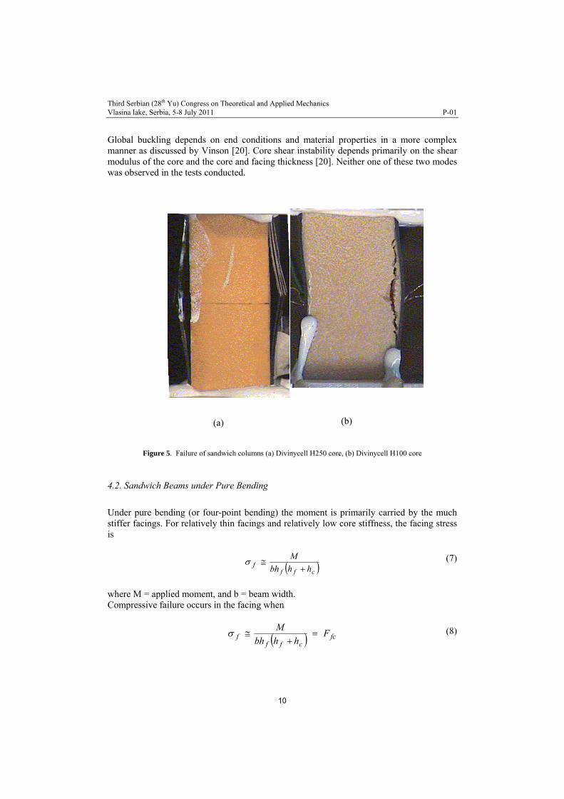
Global buckling depends on end conditions and material properties in a more complex manner as discussed by Vinson [20]. Core shear instability depends primarily on the shear modulus of the core and the core and facing thickness [20]. Neither one of these two modes was observed in the tests conducted.
(b) (a)
Figure 5. Failure of sandwich columns (a) Divinycell H250 core, (b) Divinycell H100 core
4.2. Sandwich Beams under Pure Bending
Under pure bending (or four-point bending) the moment is primarily carried by the much stiffer facings. For relatively thin facings and relatively low core stiffness, the facing stress is
cfff hhbh
M
(7)
where M = applied moment, and b = beam width. Compressive failure occurs in the facing when
fc
cfff F
hhbh
M
(8)
10

Third Serbian (28th Yu) Congress on Theoretical and Applied Mechanics Vlasina lake, Serbia, 5-8 July 2011 P-01
where Ffc = compressive strength of facing material. This mode of failure occurs in beams with cores of sufficiently high stiffness in the core direction, such as aluminum honeycomb. Fig. 6 shows experimental and predicted moment-strain curves for facings of a beam under four-point bending where the failure mode was compressive failure of the skin as predicted by Eq. (8).
Figure 6. Experimental and predicted moment-strain curves for two facings of composite sandwich beam under four-point bending (dimensions are in cm)
For lower stiffness cores, a more likely failure mode is facing wrinkling as predicted by the modified Heath expression, Eq. (6). Facing wrinkling failure will occur when the predicted critical stress by Eq. (6) is less than the compressive strength of the facing material. The value of core modulus at transition from skin wrinkling to facing compressive failure is obtained from Eqs (6) and (8) as
2fc
1f
3113
f
c3c F
E
νν1
h
h
2
3E
(9)
For values of the core modulus greater than calculated by Eq. (9), failure is governed by the compressive strength of the facing material. For core moduli lower than calculated above, facing wrinkling failure takes place and is controlled by the core modulus. Fig. 7 shows moment-strain curves for two beams with Divinycell H100 foam cores under four-point bending. Failure in both cases is due to facing wrinkling. The measured facing stress at failure is relatively close to the predicted critical wrinkling stress by Heath’s formula, Eq. (6).
0
0.5
1
1.5
0 0.2 0.4 0.6 0.8 1 1.2 1.4
Strain, (%)
Mo
men
t (k
N-m
)
Tension FacingsCompression Facings
1.6
0
2
4
6
8
10
12
Mo
men
t (k
ip-i
n)
Experimental Model (Linear Strain)
Model (Constant Strain)
2.6
2.7
P/2
40.6
P/2
17.8
11
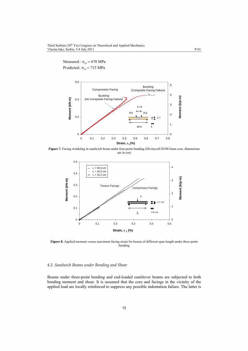
Third Serbian (28th Yu) Congress on Theoretical and Applied Mechanics Vlasina lake, Serbia, 5-8 July 2011 P-01
MPa670σ:Measured cr MPa715σ:edictedPr cr
0
0.2
0.4
0.6
0 0.1 0.2 0.3 0.4 0.5 0.6 0.7 0.8
Strain, 1 (%)
Mo
men
t (k
N-m
)
0
1
2
3
4
5
Mo
men
t (k
ip-i
n)
Compression FacingBuckling
(Composite Facing Failure)
Buckling (No Composite Facing Failure)
2.7
2.
P/2
40.6
P/2
17.8
Figure 7. Facing wrinkling in sandwich beam under four-point bending (Divinycell H100 foam core, dimensions
are in cm)
0
0.1
0.2
0.3
0.4
0.5
0 0.1 0.2 0.3 0.4 0.5
Strain, 1 (%)
Mo
me
nt
(kN
-m)
0
1
2
3
4
Mo
me
nt
(kip
-in
)
Tension FacingsCompression Facings
L = 40.6 cm L = 20.3 cm L = 10.2 cm
2.7 cm
2.6 cm
P
L
Figure 8. Applied moment versus maximum facing strain for beams of different span length under three-point bending
4.3. Sandwich Beams under Bending and Shear
Beams under three-point bending and end-loaded cantilever beams are subjected to both bending moment and shear. It is assumed that the core and facings in the vicinity of the applied load are locally reinforced to suppress any possible indentation failure. The latter is
12

Third Serbian (28th Yu) Congress on Theoretical and Applied Mechanics Vlasina lake, Serbia, 5-8 July 2011 P-01
the subject of another study [5, 9, 21]. The bending moment is primarily carried by the facings and the shear by the core. Excluding indentation, possible failure modes include core shear failure, core failure under combined shear and compression, facing wrinkling and facing compressive failure. Sandwich beams with aluminum honeycomb cores under three-point bending failed due to early shear crimping of the core. The shear force at failure remained nearly constant for varying span lengths. This means that as the span length increases, the applied maximum moment and, thereby, the maximum face sheet strains at failure increase (Fig. 8). The results also indicate that the bending moment is carried almost entirely by the face sheets. The average shear stress at failure from the three tests represented in Fig. 8 is
which compares well with the measured shear strength of the honeycomb
material of MPa59.3τu
Fc MPa59.3
Figure 9. Moiré fringe patterns corresponding to horizontal and vertical displacements in sandwich beam under three-point bending (12 lines/mm, Divinycell H250 core)
The deformation and failure mechanisms in the core were studied experimentally by means of moiré gratings and birefringent coatings. Fig. 9 shows moiré fringe patterns for the vertical, w, and horizontal, u, displacements in the core of a sandwich beam with Divinycell H250 foam core under three-point bending. They were obtained with specimen gratings of 11.8 lines/mm and a master grating of the same pitch with lines parallel to the longitudinal and vertical directions. The moiré fringe patterns of Fig. 9 corresponding to the horizontal (u) displacements away from the applied load consist of nearly parallel and equidistant fringes from which it follows that
1x Cz
u,0
x
uε
(10)
z
P
W U
13

Third Serbian (28th Yu) Congress on Theoretical and Applied Mechanics Vlasina lake, Serbia, 5-8 July 2011 P-01
where C1is a constant. Similarly, the moiré fringe patterns corresponding to the vertical (w) displacements away from the applied load consist of nearly parallel and equidistant fringes from which it follows that
22 C
x
w,0
z
wε
(11)
where C2 is constant. From Eqs (10) and (11) it follows that
x
w
z
uγxz
constant (12)
Eq. (12) indicates that the core is under nearly uniform shear strain, and therefore, under nearly uniform shear stress. Furthermore, Eqs (10) and (11) indicate that the normal strains εx and εz in the core are nearly zero or very small compared to the shear strain. This is in accordance with the classical bending theory of sandwich beams. The bending moment is taken mainly by the tensile and compressive facings. This results in high facing normal stresses with low normal strains due to the high Young’s modulus of the facings. On the other hand the shearing force is taken mainly by the core, resulting in high core strains due to the low shear modulus of the core. Thus, the core is under nearly uniform shear stress. This is true only in the linear range as shown by the isochromatic fringe patterns of the birefringent coating in Fig. 10. In the nonlinear and plastic region the core begins to yield and the shear strain becomes highly nonuniform peaking at the center. From fringe patterns like those of Fig. 10 it was found that the shear deformation starts becoming nonuniform at an applied load of 3.29 kN which corresponds to an average shear stress of 2.55 MPa. This is close to the proportional limit of the shear stress-strain curve of Fig. 3. As the load increases the shear strain in the core becomes nonuniform peaking at the center is illustrated in Fig. 4. Core failure is accelerated when compressive and shear stresses are combined. This critical combination is evident from the failure envelope of Fig. 4. The criticality of the compression/shear stress biaxiality was tested with a cantilever sandwich beam loaded at the free end. The cantilever beam was 25.4 cm long. A special fixture was prepared to provide the end support of the beam. The isochromatic fringe patterns of the birefringent coating in Fig. 10 show how the peak birefringence moves towards the fixed end of the beam at the bottom where the compressive strain is the highest and superimposed on the shear strain.
14

Third Serbian (28th Yu) Congress on Theoretical and Applied Mechanics Vlasina lake, Serbia, 5-8 July 2011 P-01
Birefringent Coating
P = 2.1 kN (474 lb) P = 2.4 kN (532 lb)
P = 2.44 kN (549 lb) P = 2.47 kN (555 lb)
P = 2.48 kN (558 lb) P = 2.47 kN (554 lb)
P
Birefringent Coating
P = 2.1 kN (474 lb) P = 2.4 kN (532 lb)
P = 2.44 kN (549 lb) P = 2.47 kN (555 lb)
P = 2.48 kN (558 lb) P = 2.47 kN (554 lb)
P
Figure 10. Isochromatic fringe patterns in birefringent coating of a cantilever sandwich beamunder end load
Plastic deformation of the core, whether due to shear alone or a combination of compression and shear, degrade the supporting role of the core and precipitate other more catastrophic failure modes, such as facing wrinkling. In the present case of beams subjected to bending and shear, compression facing wrinkling is influenced by the shear as well as the axial stiffnesses of the core in the through-the-thickness direction. A prediction of the critical facing wrinkling stress for this case was given by Hoff and Mautner [22].
3/113c3c1fcr GEEcσ (13)
where c is a constant usually taken equal to 0.5. In this relation the core moduli are the initial elastic moduli if wrinkling occurs while the core is still in the linear elastic range. This requires that the shear force at the time of wrinkling be low enough or, at least, csc FAV (14)
where Ac = core cross sectional area Fcs = core shear strength Sandwich beams with Divinycell H250 foam cores were tested under three-point bending and as cantilever beams, while monitoring strain on the face sheets, at points of highest compressive stress. Moment-strain curves for three such beams are shown in Fig. 11. The maximum moment recorded is an indication of facing wrinkling. For the cantilever beam and one of the beams loaded in three-point bending, the facing wrinkling obtained from the experiments are:
15

Third Serbian (28th Yu) Congress on Theoretical and Applied Mechanics Vlasina lake, Serbia, 5-8 July 2011 P-01
(cantilever) MPa910σcr (three-point bending) MPa715σcr The calculated value from eq. (11) is MPa945σcr In the case of the short beam the experimental critical stress at facing wrinkling is cr=500 MPa. This lower than predicted value is attributed to the fact that the shear loading component is significant and core failure precedes facing wrinkling. Core failure takes the form of core yielding, which results in reduced Young’s modulus. This reduces the core support of the facing and precipitates facing wrinkling at a lower stress. The critical wrinkling stress in this case could be predicted by a modification of expression (13) as 3/1
13c3c1fcr GEE5.0σ (15)
Figure 11. Moment-strain curves for beams in three-point bending
where and are the reduced core moduli. The determination of these moduli
would require an exact elastic-plastic stress analysis of the beam. 3cE 13cG
It is obvious from the above that failure modes, their initiation, sequence and interaction depend on loading conditions. In the case of beams under three-point bending this is illustrated by varying the span length. For short spans, core failure occurs first and then it triggers facing wrinkling. For long spans, facing wrinkling can occur before any core failure. Core failure initiation can be described by calculating the state of stress in the core and applying the Tsai-Wu failure criterion. This yields a curve for critical load (at core failure initiation) versus span length. On the other hand, in the absence of core failure,
16

Third Serbian (28th Yu) Congress on Theoretical and Applied Mechanics Vlasina lake, Serbia, 5-8 July 2011 P-01
facing wrinkling can be predicted by Eq. (11) and expressed in terms of a critical load as a function of span length. Fig. 12 shows curves of the critical load versus span length for initiation of the two failure modes discussed above. Their intersection defines the transition from core failure initiation to facing wrinkling initiation. For a beam with carbon/epoxy facings (8-ply unidirectional AS4/3501) and PVC foam core (Divinycell H250) of 2.5 x 2.5 cm cross section, the span length for failure mode transition is L = 35 cm. Although the results above are at least qualitatively explained by available theory, it is apparent that better theoretical modeling is needed. The theoretical prediction of facing wrinkling, Eq. (13), gives equal weight to the three moduli involved and is independent of facing and core dimensions. A more sound theory should take into consideration the nonlinear and inelastic biaxial stress-strain behavior of the core material and the stress/strain redistribution following core yielding.
0 25 50 7
L (cm)
Pcri
t (N
)
0
2000
4000
6000
8000
Core Failure
5
1"
1"
P
L
Facing Wrinkling
Figure 12: Critical load versus span length for initiation of core failure and facing wrinkling.
4.4 Facing debonding
Facesheet debonding may develop during fabrication of sandwich panels or may be caused by external loading such as impact. Debonding reduces the stiffness of the structure and makes it susceptible to buckling under in-plane compression. Facesheet/core debonding failures and interfacial cracking have been studied by many investigators over the last two decades by means of experimental, numerical and analytical methods [23-30]. Debonding failures are not typically observed in many sandwich beam specimens under usual quasi-static loading configurations. In the case of foam cores no debonding was observed under quasi-static loading due to the relatively high interface fracture toughness. Under impact, delamination failures of the compressive face sheet have been observed, but no interfacial debonding. Beams with aluminum honeycomb cores (Fig. 13) showed some premature debonding failure in some cases due to the very small bonded area of the honeycomb cross section.
17

Third Serbian (28th Yu) Congress on Theoretical and Applied Mechanics Vlasina lake, Serbia, 5-8 July 2011 P-01
Figure 13. Double cantilever sandwich beam specimen.
The strain energy release rate for interfacial crack growth is given by
2 2int Ι ΙΙ
1 2
1 1 1(
2
G K
E E)K (16)
where 21 j jE E j for plane strain, and jE E j for plane stress, and for crack
growth in a monolithic elastic material by
2 2Ι Ι
vol
ΙK K
GE
(17)
The interfacial crack may propagate along the interface or kink into one of the adjoining materials. The angle of initial crack propagation, Ω, is given, according to the maximum tangential (hoop) stress criterion, by:
2
II I1
II I
1 8 12tan
4
K K
K K (18)
Kinking of the interfacial crack into the core occurs when the following inequality is satisfied:
18
Third Serbian (28th Yu) Congress on Theoretical and Applied Mechanics Vlasina lake, Serbia, 5-8 July 2011 P-01
I,cr cr intcore
max
G G
G G
(19)
The critical strain energy release rate for the core material in mode I, , and the critical
interfacial strain energy release rate, I,crG
crG , as function of mode mixity, are determined
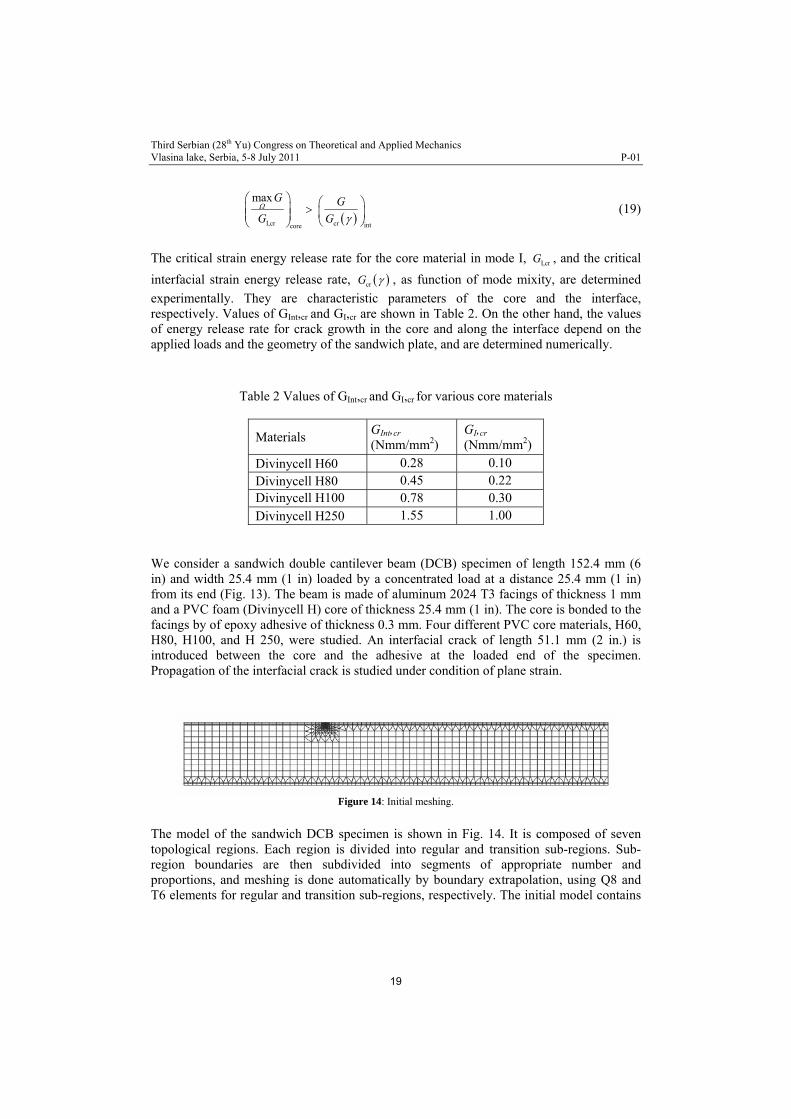
experimentally. They are characteristic parameters of the core and the interface, respectively. Values of GInt,cr and GI,cr are shown in Table 2. On the other hand, the values of energy release rate for crack growth in the core and along the interface depend on the applied loads and the geometry of the sandwich plate, and are determined numerically.
Table 2 Values of GInt,cr and GI,cr for various core materials
Materials GInt,cr (Nmm/mm2)
GI,cr (Nmm/mm2)
Divinycell H60 0.28 0.10 Divinycell H80 0.45 0.22 Divinycell H100 0.78 0.30 Divinycell H250 1.55 1.00
We consider a sandwich double cantilever beam (DCB) specimen of length 152.4 mm (6 in) and width 25.4 mm (1 in) loaded by a concentrated load at a distance 25.4 mm (1 in) from its end (Fig. 13). The beam is made of aluminum 2024 T3 facings of thickness 1 mm and a PVC foam (Divinycell H) core of thickness 25.4 mm (1 in). The core is bonded to the facings by of epoxy adhesive of thickness 0.3 mm. Four different PVC core materials, H60, H80, H100, and H 250, were studied. An interfacial crack of length 51.1 mm (2 in.) is introduced between the core and the adhesive at the loaded end of the specimen. Propagation of the interfacial crack is studied under condition of plane strain.
Figure 14: Initial meshing.
The model of the sandwich DCB specimen is shown in Fig. 14. It is composed of seven topological regions. Each region is divided into regular and transition sub-regions. Sub-region boundaries are then subdivided into segments of appropriate number and proportions, and meshing is done automatically by boundary extrapolation, using Q8 and T6 elements for regular and transition sub-regions, respectively. The initial model contains
19
Third Serbian (28th Yu) Congress on Theoretical and Applied Mechanics Vlasina lake, Serbia, 5-8 July 2011 P-01
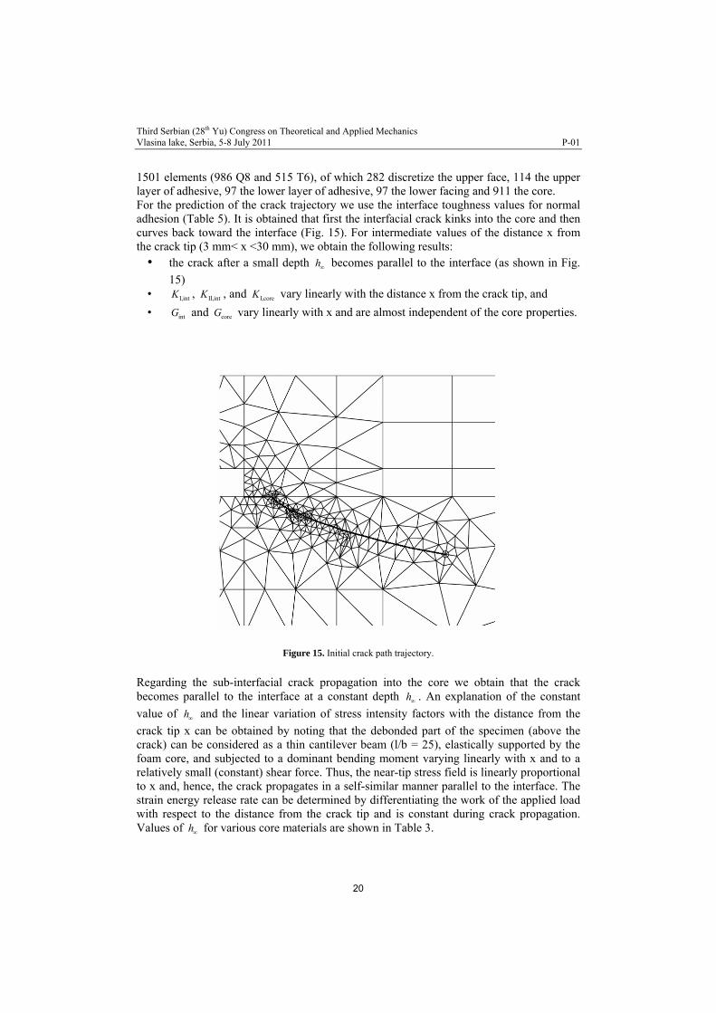
1501 elements (986 Q8 and 515 T6), of which 282 discretize the upper face, 114 the upper layer of adhesive, 97 the lower layer of adhesive, 97 the lower facing and 911 the core. For the prediction of the crack trajectory we use the interface toughness values for normal adhesion (Table 5). It is obtained that first the interfacial crack kinks into the core and then curves back toward the interface (Fig. 15). For intermediate values of the distance x from the crack tip (3 mm< x <30 mm), we obtain the following results:
• the crack after a small depth h becomes parallel to the interface (as shown in Fig.
15) • I,intK , , and vary linearly with the distance x from the crack tip, and II,intK I,coreK
• and vary linearly with x and are almost independent of the core properties. intG coreG
Figure 15. Initial crack path trajectory.
Regarding the sub-interfacial crack propagation into the core we obtain that the crack becomes parallel to the interface at a constant depth h . An explanation of the constant
value of and the linear variation of stress intensity factors with the distance from the
crack tip x can be obtained by noting that the debonded part of the specimen (above the crack) can be considered as a thin cantilever beam (l/b = 25), elastically supported by the foam core, and subjected to a dominant bending moment varying linearly with x and to a relatively small (constant) shear force. Thus, the near-tip stress field is linearly proportional to x and, hence, the crack propagates in a self-similar manner parallel to the interface. The strain energy release rate can be determined by differentiating the work of the applied load with respect to the distance from the crack tip and is constant during crack propagation. Values of for various core materials are shown in Table 3.
h
h
20

Third Serbian (28th Yu) Congress on Theoretical and Applied Mechanics Vlasina lake, Serbia, 5-8 July 2011 P-01
The core stiffness appears to be the main factor that influences the value of the asymptotic depth . Indeed, it can be obtained from Table 3 that the product h Eh is almost constant
and equal to 60 N/mm for the three PVC foam materials H60, H80 and H250. For H100 it takes the value 70 N/mm. Thus, the depth h is inversely proportional to the modulus of
elasticity of the core material. Table 3. Values of critical distance h∞
E h Eh
(GPa) (mm) (N/mm
) H 60 0.059 1.01 59.6 H 80 0.087 0.70 60.9 H 100 0.107 0.65 69.6 H 250 0.308 0.20 61.6
Under such conditions and for a critical applied load, debonding propagates along the interface only when the adhesion between the interface and the core is weak. Otherwise, the crack kinks into the core and after a small initial curved path it propagates parallel to the interface at a depth . The value of h h is inversely proportional to the modulus of
elasticity of the core. This behavior is independent of the core thickness, which is an order of magnitude larger than the thickness of the facing and the adhesive. Away from boundary effects (e.g., concentrated loads, beam supports, crack kinking, etc.) both stress intensity factors and strain energy release rate can be approximated as linear functions of the crack length.
5. Conclusions
The initiation of the various failure modes in composite sandwich beams depends on the material properties of the constituents (facings, adhesive, core), geometric dimensions and type of loading. The appropriate failure criteria should account for the complete state of stress at a point, including two- and three-dimensional effects. Failure modes were discussed according to the type of loading applied. In sandwich columns under compression, or beams in pure bending, compressive failure of the skins takes place if the core is sufficiently stiff in the through-the-thickness direction. Otherwise, facing wrinkling takes place, which can be predicted by Heath’s formula. Experimental results were close to predicted ones. In the case of beams subjected to bending and shear the type of failure initiation depends on the relative magnitude of the shear component. When the shear component is low (long beams), facing wrinkling occurs first while the core is still in the linear elastic range. The critical stress at wrinkling can be predicted satisfactorily by an expression by Hoff and Mautner and depends only on the facing and core moduli. When the shear component is
21

Third Serbian (28th Yu) Congress on Theoretical and Applied Mechanics Vlasina lake, Serbia, 5-8 July 2011 P-01
relatively high (e.g., short beams), core shear failure takes place first and is followed by compression facing wrinkling. Wrinkling failure follows but at a lower than predicted critical stress. The predictive expression must be adjusted to account for the reduced core moduli.
References [1] Allen H G (1969) Analysis and Design of Structural Sandwich Panels, Pergamon Press, London. [2] Hall D J and Robson B L (1984) A Review of the Design and Materials Evaluation Programme for the
GRP/Foam Sandwich Composite Hull of the RAN Minehunter, Composites, 15, pp 266-276. [3] Zenkert D (1995) An Introduction to Sandwich Construction, Chameleon, London. [4] Daniel, I M, Gdoutos E E, Wang, K-A and Abot J L (2002), Failure Modes of Composite Sandwich Beams,
International Journal of Damage Mechanics, 11, pp. 309-334. [5] Gdoutos E E., Daniel I M and Wang K-A (2001) Indentation Failure of Sandwich Panels," Proceedings of the 6th Greek
National Congress on Mechanics, E C Aifantis and A N Kounadis (Eds.), July 19-21, 2001, Thessaloniki, Greece, pp. 320-326.
[6] Daniel I M, Gdoutos E E and Wang K-A (2001) Failure of Composite Sandwich Beams, Proceedings of the Second Greek National Conference on Composite Materials, HELLAS-COMP 2001, Patras, Greece, 6-9 June 2001.
[7] Daniel I M, Gdoutos E E, Abot J L and Wang K-A (2001) Core Failure Modes in Composite Sandwich Beams, ASME International Mechanical Engineering Congress and Exposition, New York, November 11-16, 2001, Contemporary Research in Engineering Mechanics, G A Kardomateas and V. Birman (Eds.), AD-Vol. 65, AMD-Vol. 249, pp. 293-303.
[8] Gdoutos E E, Daniel I M, Abot J L and Wang K-A (2001) Effect of Loading Conditions on Deformation and Failure of Composite Sandwich Structures, Proceedings of ASME International Mechanical Engineering Congress and Exposition, New York, November 11 -16.
[9] Gdoutos E E, Daniel I M and Wang K-A (2001) Indentation Failure in Composite Sandwich Structures, Experimental Mechanics, 42, pp. 426-431.
[10] Daniel I M, Gdoutos E E and Wang K-A (2002) Failure of Composite Sandwich Beams, Advanced Composites Letters, 11, pp. 49-57.
[11] Abot J.L., Daniel, I M, and Gdoutos E E (2002) Failure Mechanisms of Composite Sandwich Beams Under Impact Loading, Proceedings of the 14th European Conference on Fracture, Cracow, September 8-13, 2002, edited by A. Neimitz et al, Vol. I, pp. 13-19.
[12] Abot J L, Daniel, I M and E E Gdoutos (2002) Contact Law for Composite Sandwich Beams, Journal of Sandwich Structures and Materials, 4, pp. 157-173.
[13] Gdoutos E E, Daniel I M, Wang K –A (2003) Compression Facing Wrinkling of Composite Sandwich Structures, Mechanics of Materials, 35, pp. 511-522.
[14] Daniel I M, Gdoutos E E, Abot J L and Wang K –A (2003) Core Failure of Sandwich Beams,” in “Recent Advances in Composite Materials, E E Gdoutos and Z P Marioli-Riga (Eds.), Kluwer Academic Publishers, pp. 279-290.
[15] Daniel I M, Gdoutos E E and Abot J L (2003) Optical Methods for Analysis of Deformation and Failure of Composite Sandwich Beams, Proceedings of the 2003 SEM Annual Conference, June 2-4, 2003, Charlotte, North Carolina.
[16] Hsiao H M, Daniel I M and Wooh S C (1995) A New Compression Test Method for Thick Composites, Journal of Composite Materials, 29, pp. 1789-1806.
[17] Daniel I M and Abot J L (2000) Fabrication, Testing and Analysis of Composite Sandwich Beams, Composites Science and Technology, 60, pp. 2455-2463.
[18] Gdoutos E E, Daniel I M. and Wang K-A (2002) Failure of Cellular Foams under Multiaxial Loading, Composites, Part A, 33, pp. 163-176.
[19] Heath W G (1969) Sandwich Construction, Part 2: The Optimum Design of Flat Sandwich Panels, Aircraft Engineering, 32, pp. 230-235.
[20] Vinson J R (1999) The Behavior of Sandwich Structures of Isotropic and Composite Materials, Technomic Publishing Co., Lancaster, PA, USA.
[21] Gdoutos E E, Daniel I M and Wang K-A (2001) Indentation Failure in Composite Sandwich Structures, Proceedings 2001 SEM Annual Conf., June 4-6, 2001, Portland, Oregon, USA, pp. 528-531.
[22] Hoff N J and Mautner S E (1945) The Buckling of Sandwich-Type Panels, Journal of Aerospace Sciences, 12, pp. 285-297.
[23] Prasad S and Carlsson L A (1994) Debonding and Crack Kinking in Foam Core Sandwich Beams. 1. Analysis of Fracture Specimens, Engineering Fracture Mechanics, 47, pp. 813-824.
22

Third Serbian (28th Yu) Congress on Theoretical and Applied Mechanics Vlasina lake, Serbia, 5-8 July 2011 P-01
[24] Prasad S and Carlsson L A (1994) Debonding and Crack Kinking in Foam Core Sandwich Beams. 2.
Experimental Investigation, Engineering Fracture Mechanics, 47, pp. 825-841. [25] Grau D L, Qiu X S, Sankar B V (2006) Relation Between Interfacial Fracture Toughness and Mode-Mixity in
Honeycomb Core Sandwich Composites, Journal of Sandwich Structures and Materials, 8, pp. 187-203. [26] Minakuchi S, Okabe Y and Takeda N (2007) Real-Time Detection of Debonding Between Honeycomb Core
and Facesheet Using Small Diameter FBG Sensor Embedded in Adhesive Layer, Journal of Sandwich Structures and Materials, 9, pp. 9-33.
[27] Berggreen C, Simonsen B C and Borum K K (2007) Experimental and Numerical Study of Interface Crack Propagation in Foam-Cored Sandwich Beams, Journal of Composite Materials, 41, pp. 493-520.
[28] Aviles F and Carlsson L A (2008) Analysis of the Sandwich DCB Specimen for Debond Characterization, Engineering Fracture Mechanics, 75, pp. 153-168.
[29] Østergaard R C, Sørensen B F and Brøndsted P (2007) Measurement of Interface Fracture Toughness of Sandwich Structures under Mixed Mode Loadings, Journal of Sandwich Structures and Materials, 9, pp. 445-466.
[29] Berggreen C, Simonsen B C and Borum K K (2007) Experimental and Numerical Study of Interface Crack Propagation in Foam-cored Sandwich Beams, Journal of Composite Materials, 41, pp. 493-520.
[30] Daniel I M and Gdoutos E E (2009) Failure Modes in Composite Sandwich Beams, in Major Accomplishments in Composite Materials and Sandwich Structures, Daniel I M, Gdoutos E E and Y.D.S. Rajapakse (Eds.), Springer, pp. 197-227.
23

Third Serbian (28th Yu) Congress on Theoretical and Applied Mechanics Vlasina lake, Serbia, 5-8 July 2011 P-02
Brief Review of Development of The Smooth Particle Hydrodynamics
(SPH) Method
Rade Vignjevic, James Campbell Cranfield University Crashworthiness, Impact and Structural Mechanics (CISM) [email protected]
Abstract
The paper gives an overview of developments of the SPH method. Especial attention is given to the main shortcomings of the original form of the method naimly consistency, tensile instability and zero energy modes. An example of derivation of correction necessary to assure first order consistency is given. The origin of the tensile instability and few proposed solutions to this problem are described. Similar consideration is given with respect to the zero energy modes typical for the collocational SPH method.
Introduction
This paper discusses the development of the Smooth Particle Hydrodynamics (SPH) method in its original form based on updated Lagrangian formalism. SPH is a relatively new numerical technique for the approximate integration of partial differential equations. It is a meshless Lagrangian method that uses a pseudo-particle interpolation method to compute smooth field variables. Each pseudo-particle has a mass, Lagrangian position, Lagrangian velocity, and internal energy; other quantities are derived by interpolation or from constitutive relations. The advantage of the meshless approach is its ability to solve problems that cannot be effectively solved using other numerical techniques. It does not suffer from the mesh distortion problems that limit Lagrangian approaches based on structured mesh when simulating large deformations. As it is a Lagrangian method it naturally tracks material history information, such as damage, without the diffusion that occurs in Eulerian approaches due to advection. Gingold and Lucy initially developed SPH in 1977 for the simulation of astrophysics problems. Their breakthrough was a method for the calculation of derivatives that did not require a structured computational mesh. Review papers by Benz and Monaghan (1982) cover the early development of SPH. Libersky and Petchek (1990) extended SPH to work with the full stress tensor in 2D. This addition allowed SPH to be used in problems where material strength is important. The development SPH with strength of materials continued
24

Third Serbian (28th Yu) Congress on Theoretical and Applied Mechanics Vlasina lake, Serbia, 5-8 July 2011 P-02
with extension to 3D Libersky (1993), and the linking of SPH with existing finite element codes Attaway, Johnson (1994). The introduction of material strength highlighted shortcomings in the basic method: accuracy, tensile instability, zero energy modes and artificial viscosity. These shortcomings were identified in a first comprehensive analysis of the SPH method by Swegle, Wen. The problems of consistency and accuracy of the SPH method, identified by Belytschko (1996), were addressed by Randles and Libersky (1996) and Vignjevic and Campbell (2000). This resulted in a normalised first order consistent version of the SPH method with improved accuracy. The attempts to ensure first order consistency in SPH led to the development of a number of variants of the SPH method, such as Element Free Galerkin Mehod (EFGM) Belytschko (1994), Kongauz (1997), Reproducing Kernel Particle Method (RKPM) Liu (1995, 1997), Moving Least Square Particle Hydrodynamics (MLSPH) Dilts, Meshless Local Petrov Galerkin Method (MLPG) Atluri (2000). These methods allow the restoration of consistency of any order by means of a correction function. It has been shown by Atluri that the approximations based on corrected kernels are identical to moving least square approximations. The issue of stability was dealt with in the context of particle methods in general by Belytschko (2002), and independently by Randles (1999). They reached the same conclusions as Swegle in his initial study. In spite of these improvements, the crucial issue of convergence in a rigorous mathematical sense and the links with conservation have not been well understood. Encouraging preliminary steps in this direction have already been put forward very recently by Ben Moussa, who proved convergence of their meshless scheme for non-linear scalar conservation laws; see also Ben Mousa and Vila. This theoretical result appears to be the first of its kind in the context of meshless methods. Furthermore, Ben Moussa proposed an interesting new way to stabilise normalised SPH and allow for treatment of boundary conditions by incorporating upwinding, an approach usually associated with finite volume shock-capturing schemes of the Godunov type, see Toro (1991, 1995, 1999). The task of designing practical schemes along these lines is pending, and there is scope for cross-fertilisation between engineers and mathematicians and between SHP specialists and Godunov-type schemes specialists. The improvements of the methods in accuracy and stability achieved by kernel re-normalisation or correction, have not, however, come for free; now it is necessary to treat the essential boundary conditions in a rigorous way. The approximations in SPH do not have the property of strict interpolants so that in general they are not equal to the particle value of the dependent variable, i.e. u x x u uh
j II
j I J( ) ( )
uI
. Consequently it does
not suffice to impose zero values for at the boundary positions to enforce homogeneous
boundary conditions. The treatment of boundary conditions and contact was neglected in the conventional SPH method. If the imposition of the free surface boundary condition (stress free condition) is simply ignored, then conventional SPH will behave in an approximately correct manner, giving zero pressure for fluids and zero surface stresses for solids, because of the deficiency of particles at the boundary. This is the reason why conventional SPH gives physically
25

Third Serbian (28th Yu) Congress on Theoretical and Applied Mechanics Vlasina lake, Serbia, 5-8 July 2011 P-02
reasonable results at free surfaces. Contact between bodies occurs by smoothing over all particles, regardless of material. Although simple this approach gives physically incorrect results. Campbell [30] made an early attempt to introduce a more systematic treatment of boundary condition by re-considering the original kernel integral estimates and taking into account the boundary conditions through residual terms in the integral by parts. Probably the most sophisticated work on boundary conditions in SPH is due to Takeda et al. [31], who have applied SPH to a variety of viscous flows. A similar approach has also been used to a limited extent by Libersky [8] with the ghost particles added to accomplish a reflected symmetrical surface boundary condition. In, Belytschko, Lu and Gu [19] the essential boundary conditions were imposed by the use of Lagrange multipliers leading to an awkward structure of the linear algebraic equations, which are not positive definite. Krongauz and Belytschko [32] proposed a simpler technique for the treatment of the essential boundary conditions in meshless methods, by employing a string of finite elements along the essential boundaries. This allowed for the boundary conditions to be treated accurately, but reintroduced the shortcomings inherent to structured meshes. Randles et al. [18, 33] were first to propose a more general treatment of boundary conditions based on an extension of the ghost particle method. In this, the boundary is considered to be a surface one half of the local smoothing length away from the so-called boundary particles. A boundary condition is applied to a field variable by assigning the same boundary value of the variable to all ghost particles. A constraint is imposed on the boundary by interpolating it smoothly between the specified boundary particle value and the calculated values on the interior particles. This serves to communicate to the interior particles the effect of the specific boundary condition. There are two main difficulties in this:
Definition of the boundary (surface normal at the vertices). Communication of the boundary value of a dependent variable from the boundary to
internal particles. A penalty contact algorithm for SPH was developed at Cranfield by Campbell and Vignjevic (2000). This algorithm was tested on normalised SPH using the Randles approach for free surfaces. The contact algorithm considered only particle-particle interactions, and allowed contact and separation to be correctly simulated. However tests showed that this approach often excited zero-energy modes. Another unconventional solution to the SPH tensile instability problem was first proposed by Dyka in which the stresses are calculated at the locations other than the SPH particles. The results achieved in 1D were encouraging but a rigorous stability analysis was not performed. A 2D version of this approach was investigated by Vignjevic (2000), based on the normalised version of SPH. This investigation showed that extension to 2D was possible, although general boundary condition treatment and simulation of large deformations would require further research. To utilise the best aspects of the FE and SPH methods it was necessary to develop interfaces for the linking of SPH nodes with standard finite element grids (see Johnson,
26

Third Serbian (28th Yu) Congress on Theoretical and Applied Mechanics Vlasina lake, Serbia, 5-8 July 2011 P-02
(1993, 1994) and contact algorithms for treatment of contact between the two particles and elements De Vuyst and Vignjevic . From the review of the development of meshless methods, given above, the following major problems can be identified: consistency, stability and the treatment of boundary conditions. Basic Formulation
The spatial discretisation of the state variables is provided by a set of points. Instead of a grid, SPH uses a kernel interpolation to approximate the field variables at any point in a domain. For instance, an estimate of the value of a function ( )f x at the location x is
given in a continuous form by an integral of the product of the function and a kernel (weighting) function : ( ',W x x h )
( ) ( ') ( ', ) 'f x f x W x x h d x (1)
Where: the angle brackets denote a kernel approximation
h is a parameter that defines size of the kernel support known as the smoothing length 'x is new independent variable.
The kernel function usually has the following properties:
- Compact support, which means that it’s zero everywhere but on a finite domain inside the range of the smoothing length 2h:
( ', )W x x h 0 for ' 2x x h
1
(2)
- Normalised
( ', ) 'W x x h dx (3)
These requirements, formulated by Lucy (1977), ensure that the kernel function reduces to the Dirac delta function when tends to zero: h
0lim ( ', ) ( ', )h
W x x h x x h
(4)
And therefore, it follows that:
0lim ( ) ( )h
f x f x
(5)
If the function ( )f x is only known at discrete points, the integral of equation 5.1 can
be approximated by a summation:
N
1
( ) ( ) ( , )jN
jj
j
m jf x f x W x x
h (6)
where j
j
m
is the volume associated to the point or particle j . In SPH literature, the term
particles is misleading as in fact these particles have to be thought of as interpolation points rather than mass elements.
27

Third Serbian (28th Yu) Congress on Theoretical and Applied Mechanics Vlasina lake, Serbia, 5-8 July 2011 P-02
Equation 6 constitutes the basis of SPH method. The value of a variable at a particle, denoted by superscript i , is calculated by summing the contributions from a set of neighbouring particles (Figure 1), denoted by superscript j and for which the kernel
function is not zero:
1
( ) ( ) ( , )jN
i j ij
j
m jf x f x W x
x h (7)
Figure 1: Set of neighbouring particles Conservation Equations The conservation equations in Lagrangian framework are given by:
vd
dt x
(8)
1dv
dt x
or 2
dv
dt x x
(9a) and (9b)
vdE
dt x
or
2 2
vvdE
dt x x
(10a) and (10b)
with dx
vdt
The subscripts α and β denote the component. Equations 9b and 10b are the forms proposed by Monaghan (1983). The kernel interpolation allows the derivation of the basic SPH form of these conservation equations as:
'' '
'
vdW d
dt x
x (11)
28

Third Serbian (28th Yu) Congress on Theoretical and Applied Mechanics Vlasina lake, Serbia, 5-8 July 2011 P-02
2
' ' ''
' ' ' '
dvW dx W
dt x x
'dx (12)
2 2
' '' ' ''
' ' ' '
vvdEW dx W
dt x x
''dx
(13)
All the equations above contain integrals of the form: ( ')
( ') ''
g xW f x dx
x
(14)
Using a development in a Taylor series about 'x x , it follows:
( ') ( ) ( )( ') ' ( ) ( ') ( ) ... '
'
g x g x d g xW f x dx f x x x f x W dx
x x dx x
(15)
As W is an even function, the terms containing odd powers of 'x x vanish. Neglecting second and higher order terms, which is consistent with the overall order of the method, gives:
'
( ') ( ')( ') ' ( ')
' ' x x
g x g xW f x dx f x
x x
(16)
Substituting ( )g x
x
for ( )g x
x
gives:
'
( ') ( ')( ') ( ) '
' 'x x
g x g xf x f x W
x x
dx (17)
Using the last relation in equations 5.11, 5.12 and 5.13 gives
''
'
vdW d
dt x
x (18)
2
' ''
' ' '
dvW dx W
dt x x
'dx (19)
2 2
' ' ''
' '
vvdEW dx W
dt x x
'dx
(20)
All equations include kernel approximations of spatial derivatives:
( ) ( ')'
'
f x f xW d
x x
x (21)
Integrating by part gives:
( )( ) ( ) '
'
f x WW f x f x dx
x
x (22)
29

Third Serbian (28th Yu) Congress on Theoretical and Applied Mechanics Vlasina lake, Serbia, 5-8 July 2011 P-02
The first term of the second member can be rewritten:
( ')( ) '
'
W f xW f x dx
x
(23)
Using Green’s theorem, it follows:
( ')' ( ')
' i
S
W f xdx W f x n dS
x
(24)
The surface integral is zero if the domain of integration is larger than the compact support of W or if the field variable assumes zero value on the boundary of the body (free surface). If none of these conditions is satisfied, modifications should be made to account for boundary conditions. One should note that in Equations 18, 19 and 20 the spatial derivatives of the field variables are substituted by the derivatives of the kernel:
( ')' ( ) ' (25)
' '
f x WW dx f x dx
x x
It follows:
' ''
d Wv d
dt x
x (26)
2
'' '
' ' '
dv W Wdx dx
dt x x
'
(27)
2 2' ' ' ' '
' '
vdE W Wv dx d
dt x x
x
(28)
The final step is to convert the continuous volume integrals to sums over discrete interpolation points. Finally, after a few arrangements in order to improve the consistency between all equations, the most common form of the SPH discretised conservation equations are obtained:
1
i jNi j i
jj
d mv v
dt x
ij
i
W
(29)
2 21
j ii ijNj
j i ij
dv Wm
dt x
(30)
21
ii ijNj j i
ij
dE Wm v v
dt x
i
(31)
where ),( hxxWW jiij Kernel Function
30

Third Serbian (28th Yu) Congress on Theoretical and Applied Mechanics Vlasina lake, Serbia, 5-8 July 2011 P-02
To complete the discretisation one has to define the kernel function. Numerous possibilities exist. A large number of kernel function types are discussed in literature, ranging from polynomial to Gaussian. The most common is the B-spline kernel that was proposed by Monaghan (1983):
2 3
3
3 31 1
2 4
1( , ) 2 1 2
40
D
v v v
CW v h v v
hotherwise
(32)
where
'x xv
h
,
D is the number of dimensions of the problem (i.e. 1, 2 or 3), C is the scaling factor which depends on the number of dimensions and ensures that the consistency conditions 2 and 3 are satisfied:
21
310
271
3
D
C
D
D (33)
Variable Smoothing Length If large deformations occur, particles can largely separate from each other. If the smoothing length remains constant, the particle spacing can become so large than particles will no more interact. On the other hand, in compression, a lot of particles might enter in the neighbouring of each other, which can significantly slow down the calculation. In order to avoid these problems, Benz (1990) proposed the use of a variable smoothing length. The intent was to maintain a healthy neighbourhood as continuum deforms. The equation for evolution of h derived by Benz (1990) is:
1
00
n
h h
(34)
where and 0h 0 are initial smoothing length and density and is the number of
dimensions of the problem.
n
Another frequently used equation of evolution based on conservation of mass is:
31

Third Serbian (28th Yu) Congress on Theoretical and Applied Mechanics Vlasina lake, Serbia, 5-8 July 2011 P-02
1
div( )dh
h vdt n
(35)
where div is the divergence of velocity. . ( )v Neighbour Search An important step in the SPH computation is the neighbour search. This task can be extremely time consuming. The neighbour search routine lists the particles that are inside the neighbourhood of each particle at each time step. A direct search between every particle is particularly inefficient. A bucket sort algorithm is more efficient. In this method, an underlying grid of side 2h is generated and the particles are sorted according to the box in which they are located (Figure 2). Then for each particle, the neighbours are searched among the particles contained in the same box and the surrounding boxes. This allows the computational time to be cut down from a default time proportional to N² for a direct search to NlogN, where N is the total number of particles.
Figure 2: Bucket sort and neighbour search SPH Shortcomings The basic SPH method has shown several problems when used to model a solid body:
- Consistency - Tensile instability - Zero-energy modes
Consistency The SPH method in its continuous form is inconsistent within 2 h of the domain boundaries due to the kernel support incompleteness. In its discrete form the method loses its 0th order consistency not only in the vicinity of boundaries but also over the rest of the domain if particles have an irregular distribution. Meglicki (1995) showed that node disorder results
32

Third Serbian (28th Yu) Congress on Theoretical and Applied Mechanics Vlasina lake, Serbia, 5-8 July 2011 P-02
in a systematic error. Therefore, a proper SPH grid should be as regular as possible and not contain large discrepancies in order to perform most accurate simulation. The first order consistency of the method can be achieved in two ways. Firstly, by correcting the kernel function, second, by correcting the discrete form of the convolution integral of the SPH interpolation. Johnson (1996) uses this correction procedure and proposed the Normalised Smoothing Function. Vignjevic (1999) also implemented a kernel normalisation and correction to lead to a Corrected Normalised Smooth Particle Hydrodynamics (CNSPH) method which is first order consistent. The full derivation of this correction is given below. In SPH methods based on a corrected kernel, it is no-longer possible to ignore boundary conditions. In basic SPH, free surface boundary conditions are not imposed and are simply ignored as variables tends to zero at boundaries because of the deficiency of neighbour particles. Derivation of Normalised Corrected Gradient SPH formula The approximation of fields using a Normalised Corrected SPH (NCSPH) interpolation has been published Libersky&Randles (1999), Vignjevic (2000), Bonet (2000). Some authors have chosen to use properties of the integrals of motion (linear and angular momentum) to derive Normalisation and Gradient Correction for kernel interpolation, see Bonet. This approach lacks generality and does not provide the insight into the origin and the nature of the problem. A full derivation of the correction proposed by Vignjevic (2000), which has not been published before, is given below. The derivation is based on the homogeneity and isotropy of space, the space properties, which have as a consequence conservation of linear and angular momentum, see Landau. The mixed correction insures that homogeneity and isotropy of space are preserved in the process of spatial discretisation. An interpolation technique should not affect homogeneity of space. One way of demonstrating this is to prove that the interpolation of the solution space itself is independent of a translation of the coordinate axes. In order to express this statement mathematically one can start by writing the general expression for the SPH interpolation of a vector field:
j
jijj
j Wm
i
xxxFxFxx
(36)
If the field to be interpolated is the solution space then xF
and Equation 36 becomes:
jjij
j
j Wm
i
xxxxxx
(37)
In a different, translated coordinate system, this equation is:
jjij
j
j Wm
i
xxxxxx
(38)
33

Third Serbian (28th Yu) Congress on Theoretical and Applied Mechanics Vlasina lake, Serbia, 5-8 July 2011 P-02
oWhere is the coordinate vector in the new coordinate system. If the translation vector by which the origin f the coordinate system was moved is defined as
x
x
then the r lationship between xe
and x
is: xxx
(39) If the interpolated coordinates of a point are independent of the translation of coordinate axes then the following should hold:
xΔxx
(40)
By substituting Equation 40 into Equation 39 for both ix
and jx
one obtains:
j
jij
j
jjij
j
j Wm
Wm
xxxxxxx (41)
or
j
jij
j Wm
xxxxx (42)
By comparison of Equation 42 and Equation 40 it is clear that the discretised space will only be homogeneous if the following condition is satisfied:
1Wm
jji
j
j xx
(43)
Similarly, an interpolation technique should not affect isotropy of space. One way of demonstrating this is to prove that the interpolation of the solution space itself is independent of a rotation of the coordinate axes. The same holds for the SPH approximation. The change in coordinates due to a rotation of the coordinate axes is:
xCx
(45) where C is the rotation matrix. For small rotations this can also be written as:
xxx
(46)
where
is the rotation vector.
If one wants to ensure that the SPH approximation does maintain the fact that space is isotropic then the approximation has to satisfy the following condition:
xCxCx
(47)
or
CC (48)
34

Third Serbian (28th Yu) Congress on Theoretical and Applied Mechanics Vlasina lake, Serbia, 5-8 July 2011 P-02
This means that the rotation matrix has to be approximated exactly. In order to develop this equation one can start by rewriting
xI
xx
xxx
xxx
x
x (49)
where is a skew-symmetric matrix: x
0
0
0
xy
xz
yzx (50)
This means that, for small rotations, the rotation matrix is given by:
xIC (51)
The approximation of the rotated coordinates is:
xIxCxCx x (52)
This means that the requirement on the interpolation is:
xx II (53)
or
xx (54)
Expanding this expression leads to:
35

Third Serbian (28th Yu) Congress on Theoretical and Applied Mechanics Vlasina lake, Serbia, 5-8 July 2011 P-02
jjij
j
jx
jjij
x
j
j
jjij
j
jx
xxWxm
xxWxm
xxWxm
(55)
Therefore to preserve space isotropy, i.e. xx the following condition has to be
satisfied.
I
jjij
j
j xxWxm
(56)
The form of the normalised kernel function and the approximation of the first order derivatives which provides first order consistency is given in Table 1. below. Space Homogeneity Space Anisotropy Condit.
1),(1
hxxWmnnbr
jji
j
j
1x
),(1
hxxWmnnbr
jjij
j
j
Normalised - Corrected
),(
),(~
1
hxxWm
hxxWW nnbr
jji
j
j
jiij
1
1
~~~~
nnbr
jijj
j
jijij x
mWWW
Table 1. Corrected forms of the kernel function and its gradient Using the NCSPH approximations the conservation equations assume the following form:
nnbr
jijij
j
jii
m
1
~~Wvv
(57)
ij
nnbr
j j
j
i
ijm W
σσv i
~~
122
(58)
nnbr
jijijj
i
i me1
2
~~Wvv
σ
(59)
36
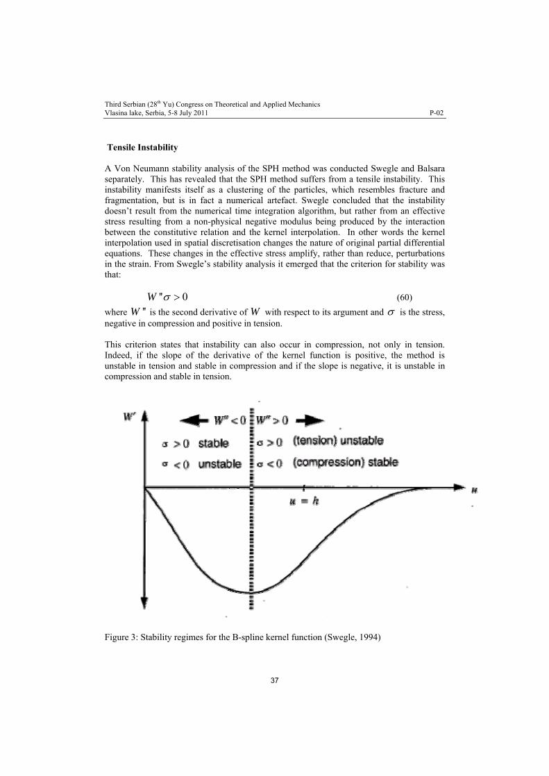
Third Serbian (28th Yu) Congress on Theoretical and Applied Mechanics Vlasina lake, Serbia, 5-8 July 2011 P-02
Tensile Instability A Von Neumann stability analysis of the SPH method was conducted Swegle and Balsara separately. This has revealed that the SPH method suffers from a tensile instability. This instability manifests itself as a clustering of the particles, which resembles fracture and fragmentation, but is in fact a numerical artefact. Swegle concluded that the instability doesn’t result from the numerical time integration algorithm, but rather from an effective stress resulting from a non-physical negative modulus being produced by the interaction between the constitutive relation and the kernel interpolation. In other words the kernel interpolation used in spatial discretisation changes the nature of original partial differential equations. These changes in the effective stress amplify, rather than reduce, perturbations in the strain. From Swegle’s stability analysis it emerged that the criterion for stability was that:
'' 0W (60)
where is the second derivative of with respect to its argument and ''W W is the stress, negative in compression and positive in tension. This criterion states that instability can also occur in compression, not only in tension. Indeed, if the slope of the derivative of the kernel function is positive, the method is unstable in tension and stable in compression and if the slope is negative, it is unstable in compression and stable in tension.
Figure 3: Stability regimes for the B-spline kernel function (Swegle, 1994)
37
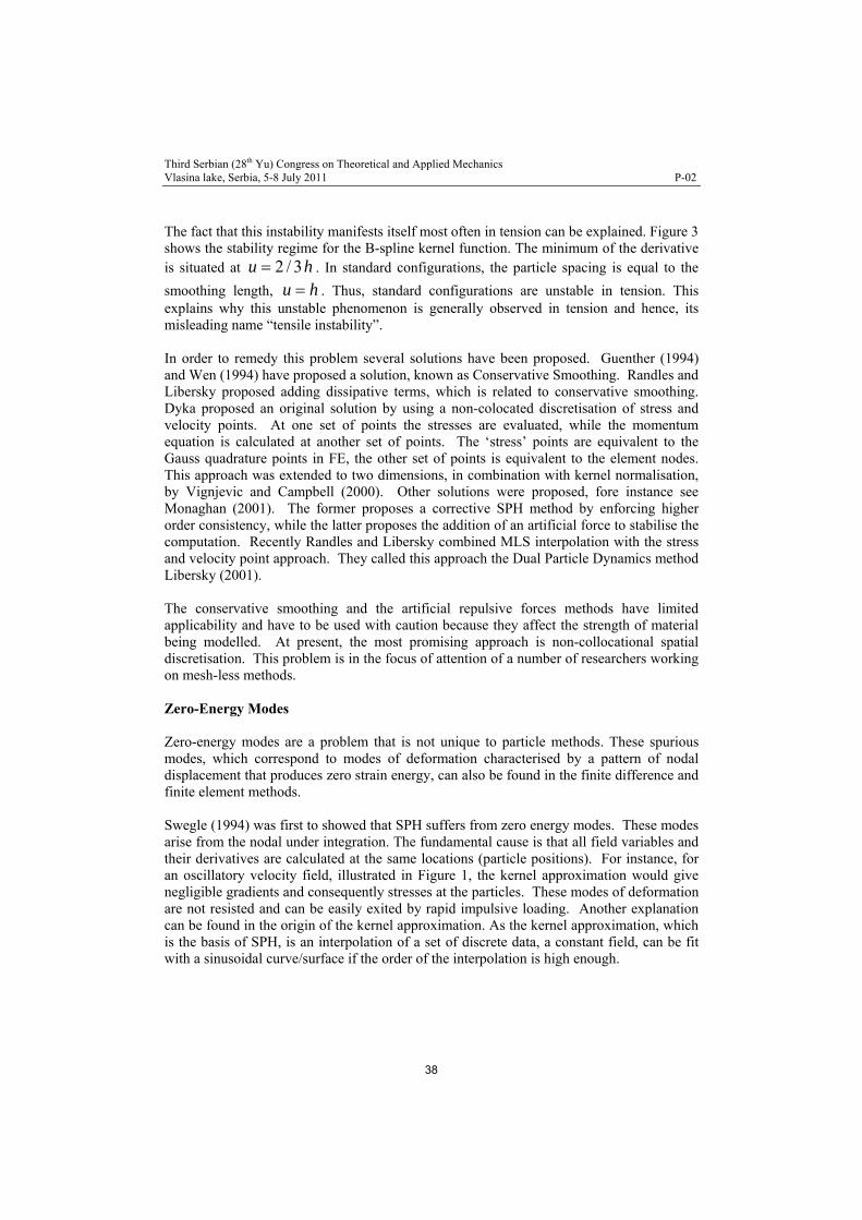
Third Serbian (28th Yu) Congress on Theoretical and Applied Mechanics Vlasina lake, Serbia, 5-8 July 2011 P-02
h
The fact that this instability manifests itself most often in tension can be explained. Figure 3 shows the stability regime for the B-spline kernel function. The minimum of the derivative is situated at 2 / 3u . In standard configurations, the particle spacing is equal to the
smoothing length, u . Thus, standard configurations are unstable in tension. This explains why this unstable phenomenon is generally observed in tension and hence, its misleading name “tensile instability”.
h
In order to remedy this problem several solutions have been proposed. Guenther (1994) and Wen (1994) have proposed a solution, known as Conservative Smoothing. Randles and Libersky proposed adding dissipative terms, which is related to conservative smoothing. Dyka proposed an original solution by using a non-colocated discretisation of stress and velocity points. At one set of points the stresses are evaluated, while the momentum equation is calculated at another set of points. The ‘stress’ points are equivalent to the Gauss quadrature points in FE, the other set of points is equivalent to the element nodes. This approach was extended to two dimensions, in combination with kernel normalisation, by Vignjevic and Campbell (2000). Other solutions were proposed, fore instance see Monaghan (2001). The former proposes a corrective SPH method by enforcing higher order consistency, while the latter proposes the addition of an artificial force to stabilise the computation. Recently Randles and Libersky combined MLS interpolation with the stress and velocity point approach. They called this approach the Dual Particle Dynamics method Libersky (2001). The conservative smoothing and the artificial repulsive forces methods have limited applicability and have to be used with caution because they affect the strength of material being modelled. At present, the most promising approach is non-collocational spatial discretisation. This problem is in the focus of attention of a number of researchers working on mesh-less methods. Zero-Energy Modes Zero-energy modes are a problem that is not unique to particle methods. These spurious modes, which correspond to modes of deformation characterised by a pattern of nodal displacement that produces zero strain energy, can also be found in the finite difference and finite element methods. Swegle (1994) was first to showed that SPH suffers from zero energy modes. These modes arise from the nodal under integration. The fundamental cause is that all field variables and their derivatives are calculated at the same locations (particle positions). For instance, for an oscillatory velocity field, illustrated in Figure 1, the kernel approximation would give negligible gradients and consequently stresses at the particles. These modes of deformation are not resisted and can be easily exited by rapid impulsive loading. Another explanation can be found in the origin of the kernel approximation. As the kernel approximation, which is the basis of SPH, is an interpolation of a set of discrete data, a constant field, can be fit with a sinusoidal curve/surface if the order of the interpolation is high enough.
38

Third Serbian (28th Yu) Congress on Theoretical and Applied Mechanics Vlasina lake, Serbia, 5-8 July 2011 P-02
Figure 4 illustrates this spurious mode for a field in 1D SPH. If one would approximate the derivative of the field shown in Figure 4 with a central difference formula:
1i1i
1i1i
xx xx
xfxf
dx
df
i
(61)
then one would obtain:
0dx
df
ixx
(62)
at all points. Hence this mode can not be detected, and can grow unhindered. This means that this mode could grow to a level where it dominates the solution.
Figure 4: Zero Energy Modes. Zero energy or spurious modes are characterised by a pattern of nodal displacement that is not a rigid body but produces zero strain energy. One of the key ideas to reduce spurious oscillations is to compute derivatives away from the particles where kernel functions have zero derivatives. Randles (1999) proposed a stress point method. Two sets of points are created for the domain discretisation, one carries velocity, and another carries stress. The velocity gradient and stress are computed on stress points, while stress divergence is sampled at the velocity points using stress point neighbours. According to Swegle (1994), these spurious modes can be eliminated by replacing the strain measure by a non-local approximation based on gradient approach. Beissel (1996) proposed another way to stabilise nodal integration, the least square stabilisation method.
39

Third Serbian (28th Yu) Congress on Theoretical and Applied Mechanics Vlasina lake, Serbia, 5-8 July 2011 P-02
Summary The paper gives an overview of developments of the SPH method. Especial attention is given to the main shortcomings of the original form of the method naimly consistency, tensile instability and zero energy modes. An example of derivation of correction necessary to assure first order consistency is given. The origin of the tensile instability and few proposed solutions to this problem are described. Similar consideration is given with respect to the zero energy modes typical for the collocational SPH method. References Atluri S., T. Zhu. (2000) A new mesless Local Petrov Galerkin (MLPG) approach in computational mechanics, Computational Mechanics, Vol 22, pp 117-127 Atluri S., H. G. Kim, J. Y. Cho, (2000)A critical assessment of the truly mesless local Petrov Galerkin (MLPG) and local boudary integral equation (LBIE), Computational Mechanics, Vol 24, pp 348-372 Attaway S. W., M.W. Heinstein, and J.W. Swegle. (1994) Coupling of smooth particle hydrodynamics with the finite element method. Nuclear Engineering and Design, 150:199—205. Beissel, S. and Belytschko, T. (1996). Nodal integration of the element-free Galerkin method. Computational Methods Applied Mechanical Engineering, Vol. 139 , pp. 49–71. Belytschko T., Y. Krongauz, D. Organ, M. Fleming, P. Krysl. (1996) Meshless Methods: An overview and recent developments Computer methods in applied mechanics and engineering, 139:3--47. Belytschko T., Y.Y. Lu, and L. Gu. (1994) Element-free Galerkin methods. International Journal for Numerical methods in Engineering, 37:229--256, 1994. Belytschko T., Xiao S. (2002), ‘Stability Analysis of Particle Methods with Corrected Derivatives’, http://www.tam.northwestern.edu/xiaop/stable.html Benz, W. (1990). Smooth particle hydrodynamics: a review. In J.R. Buchler, editor, The Numerical Modelling of Nonlinear Stellar Pulsatations, pp. 269-288. Kluwer Academic Publishers. Cited in: Camplbell, J. (1998). Lagrangian hydrocode modelling of hypervelocity impact on spacecraft. PhD thesis, Cranfield University. Bonet, J. and Kulasegaram, S. (1999). Correction and stabilization of smooth particle hydrodynamics methods with application in metal forming simulation. International Journal of Numerical Methods Engineering, Vol. 47, pp. 1189–1214. Campbell J., R. Vignjevic, L. Libersky: (2000) A Contact Algorithm for Smoothed Particle Hydrodynamics, Computer Methods in Applied Mechanics and Engineering, Vol. 184/1, pp 49-65, March 2000. Campbell P. M. (1989). Some new algorithms for boundary value problems in smooth particle hydrodynamics. Technical Report DNA-TR-88-286, Mission Research Corporation. Dilts G. A. (1997). Moving –least squares-particle hydrodynamics I, consistency and stability. Submited to International Journal for Numerical Methods in Engineering. Dyka C. T. and R.P. Ingel. (1995). An approach for tension instability in smoothed particle hydrodynamics (SPH). Computers and Structures, 57(4):573--580. Gingold, R.A. and Monaghan, J.J. (1977). Smoothed particle hydrodynamics: theory and application to non-spherical stars. Monthly Notices Royal Astronomical Society, Vol. 181, pp. 375-389.
40

Third Serbian (28th Yu) Congress on Theoretical and Applied Mechanics Vlasina lake, Serbia, 5-8 July 2011 P-02
Guenther, C., Hicks, D.L. qnd Swegle, J.W. (1994). Conservative smoothing versus artificial viscosity. Technical Report SAND94-1853. Harten A., P. D. Lax P. D.. and van Leer B., (1983). On upstream differencing and Godunov-type schemes for hyperbolic conservation laws, SIAM Review, V 25, no 1, pp 35 –61. Hughes T. J. R. (1987). The finite element method, Prentice Hall. Johnson, G.R., Petersen, E.H. and Stryk, R.A. (1993). Incorporation of an SPH option in the EPIC code for a wide range of high velocity impact computations. International Journal of Impact Engineering, Vol. 14, pp. 385-394. Johnson, G.R. (1994). Linking of Lagrangian particle methods to standard finite element methods for high velocity impact computations Nuclear Engineering and Design, Vol. 150, pp. 265-274. Johnson G. R. and S.R. Beissel. (1996). Normalised smoothing functions for SPH impact computations. International Journal for Numerical Methods in Engineering, 39:2725--2741. Johnson, G.R., Stryk, R.A. and Beissel, S.R. (1996). SPH for high velocity impact computations. Computer Methods in Applied Mechanics and Engineering, Vol. 139, pp. 347-373. Krongauz Y., Belytschko T. (1997). Enforcement of essential boundary conditions in measles approximations using finite elements. Submited to International Journal for Numerical Methods in Engineering. Krongauz Y., Belytschko T. (1997). Consitent pseudo derivatives in meshless methods Computer methods in applied mechanics and engineering, 146:371--386. Landau L. D. Lifshitz E.M. (1960). Mechanics, Course of Theoretical Physics, V 1, Pergamon Press Lattanzo J. C., J.J. Monaghan, H. Pongracic, P. Schwarz. (1996). Controlling penetration. SIAM, Journal for Scientific and Statistic Computation, V 7, No 2, pp 591—598. Libersky, L.D. and Petschek, A.G. (1990). Smooth particle hydrodynamics with strength of materials. Advances in the Free Lagrange Method, Lecture Notes in Physics, Vol. 395, pp. 248-257. Libersky, L.D., Petschek, A.G., Carney, T.C., Hipp, J.R. and Allahdadi, F.A. (1993). High Strain Lagrangian Hydrodynamics: A Three-Dimensional SPH Code for Dynamic Material Response, Journal of Computational Physics, Vol. 109, Issue 1, November, pp. 67-75. Lucy, L.B. (1977). A numerical approach to the testing of fusion process. Astronomical journal, Vol. 88, pp. 1013-1024. Meglicki, Z., Analysis and Application of Smoothed Particle Magnetohydrodynamics. PhD thesis, Australian National Univerty. Cited in Campbell, J. (1998).Lagrangian hydrocode modelling of hypervelocity impact on spacecraft. Cranfield University, College of Aeronautics, PhD thesis. Mitchell A. R. and D. F. Griffits, (1980). The finite difference method in partial differential equations, John Wiley. Monaghan J.J. (1982) Why particle methods work. SIAM Journal on Scientific and Statistical Computing, 3(4):422--433 Monaghan, J.J. and Gingold, R.A. (1983). Shock simulation by the particle method SPH. Journal of Computational Physics, Vol. 52, pp. 374-389. Monaghan, J.J. and Lattanzio, J.C. (1985). A refined particle method for astrophysical problems. Astronomy and Astrophysics, Vol. 149, Issue 1, pp. 135-143.
41

Third Serbian (28th Yu) Congress on Theoretical and Applied Mechanics Vlasina lake, Serbia, 5-8 July 2011 P-02
Monaghan and H. Pongracic (1985). Artificial viscosity for particle methods. Applied Numerical Mathematics, 1:187—194. Monaghan J.J. (1989). On the problem of penetration in particle methods. Journal of Computational Physics, 82:1--15, 1989. Monaghan J.J. (1992). Smoothed Particle Hydrodynamics. Annual Review of Astronomy and Astrophysics, 30:543--574, 1992. Monaghan, J.J. (2002). SPH without a Tensile Instability. Journal of Computational Physics, Vol. 159, pp. 290-311. Moussa B., Meshless (2000). Particle methods: Recent developments for non-linear conservation laws in bounded domain, in Godunov Methods: Theory and Applications, E. F. Toro (Editor), Kluwer Academic/Plenum Publishers. Moussa B., J. P. Vila, (2000). Convergence of the SPH method for scalar nonlinear conservation laws, SIAM Journal of Numerical Analysis, Vol 37 number 3, pp 863-887. Petschek, A.G. and Libersky, L.D. (1993). Cylindrical smoothed particle hydrodynamics. Journal of Computational Physics, Vol. 109, pp. 76-83. Randles P. W. and L.D. Libersky. (1996). Smoothed particle hydrodynamics: Some recent improvements and applications. Computer methods in applied mechanics and engineering, 139:375—408. Randles, P.W., Libersky, L.D. and Petschek, A.G. (1999). On neighbors, derivatives, and viscosity in particle codes, in: Proceedings of ECCM Conference, Munich, Germany, 31 August–3 September. Resnyansky, A. D. (2002). DYNA-modelling of the high-velocity impact problems with a split-element algorithm, International Journal of Impact Engineering, Vol. 27, Issue 7, pp. 709-727. Stryk R. A. (1996). G.R. Johnson and S.R. Beissel. SPH for high velocity impact computations. Computer methods in applied mechanics and engineering, 139:347--373. Swegle, J.W., Attaway, S.W., Heinstein, M.W., Mello, F.J. and Hicks, D.L. (1994). An analysis of smooth particle hydrodynamics. Sandia Report SAND93-2513. Takeda H. T., S. M. Miyama, M. Sekiya. (1994). Numerical simulation of viscous flow by smooth particle hydrodynamics, Progress of Theoretical Physics, 92 pp 939—960. Toro E. F., (1991). A Linearised Riemann Solver for the time dependent Euler equations of gas dynamics, Proc. Roy. Soc. London, V A434, pp 683—693. Toro E. F., (1995). Direct Riemann solvers for the time-dependent Euler equations, Shock Waves, V 5, pp 75-80. Toro E. F., (1999). Riemann Solvers and Numerical Methods for Fluid Dynamics, Second edition, Springer Verlag. Van der Vegt LJ. J. W., H van der Ven and O. J. Boelens, (1995). Discontinuous galerkin methods for partial differential equations, in Godunov Methods: Theory and Applications. Vignjevic R., J. Campbell, L. Libersky. (2000). A Treatment of Zero Energy Modes in the Smoothed Particle Hydrodynamics Method, Computer Methods in Applied Mechanics and Engineering, Vol. 184/1, pp 67-85. Vignjevic, R., De Vuyst, T., Campbell, J. (2002a). The use of a homogeneous repulsive force for contact treatement in SPH. Fifth World Congress on Computational Mechanics, Vienna, Austria, July 7-12 Vignjevic, R., Hughes, K. and Taylor E.A. (2002b). Finite element modelling of failure of a multi-material target due to high velocity space debris impacts. Space Debris, Vol. 2, pp. 41-50.
42
Third Serbian (28th Yu) Congress on Theoretical and Applied Mechanics Vlasina lake, Serbia, 5-8 July 2011 P-02
Vignjevic R., De Vuyst T., Gourma M. (2001), Interpolation Techniques in Meshless Methods, Computer Modelling in Engineering and Science Journal, V 2, No. 3, pp 319-337. Wen, Y., Hicks, D.L. and Swegle, J.W. (1994). Stabilising SPH with conservative smoothing. Technical Report SAND94-1932. Liu W. L., S. Jun, S. Li, J. Adee, and T. Belytschko. (1995). Reproducing kernel particle methods for structural dynamics. International Journal for Numerical Methods in Engineering, 38:1655--1679. Liu W. L., S. Jun, S. Li, J. Adee, and T. Belytschko. (1997) Reproducing kernel particle methods for nearly incompressible hyperelastic solids. Submited to International Journal for Numerical Methods in Engineering Bibliography Campbell, J. and Vignjevic, R. (1997). Development of lagrangian hydrocode modelling for debris impact damage prediction. International Journal of Impact Engineering, Vol. 20, pp. 143-152. MCM (2002). A 1D/2D/3D Meshless Continuum Mechanic Code for solid and fluid mechanics. User Manual. Scholl of Engineering, Cranfield University. Version 2.0. August 2002. Campbell, J. (1998). Lagrangian hydrocode modelling of hypervelocity impact on spacecraft. PhD thesis, College of Aeronautics, Cranfield University.
43

Third Serbian (28th Yu) Congress on Theoretical and Applied Mechanics Vlasina lake, Serbia, 5-8 July 2011 P-03
STABILITY OF FRACTIONAL ORDER TIME DELAY SYSTEMS
M.P.Lazarević University of Belgrade, Faculty of Mechanical Engineering, Department of Mechanics; Kraljice Mrije 16, 11020 Belgrade 35,Serbia e-mail: [email protected]
Abstract. In this paper, some basic results of the stability criteria of fractional order system with time delay as well as free delay are presented. Also, they are obtained and presented sufficient conditions for finite time stability for (non)linear (non)homogeneous as well as perturbed fractional order time delay systems. Several stability criteria for this class of fractional order systems are proposed using a recently suggested generalized Gronwall inequality as well as “classical” Bellman-Gronwall inequality. Some conclusions for stability are similar to that of classical integer-order differential equations. Last, a numerical example is given to illustrate the validity of the proposed procedure.
1. Introduction The question of stability is of main interest in control theory. Also, the problem of investigation of time delay system has been exploited over many years. Delay is very often encountered in different technical systems, such as electric, pneumatic and hydraulic networks, chemical processes, long transmission lines, etc.,[1]. Delays are inherent in many physical and engineering systems. In particular, pure delays are often used to ideally represent the effects of transmission, transportation, and inertial phenomena. This is because these systems have only limited time to receive information and react accordingly. Such a system cannot be described by purely differential equations, but has to be treated with differential difference equations or the so called differential equations with difference variables. Delay differential equations (DDEs) constitute basic mathematical models for real phenomena, for instance in engineering, mechanics, and economics, [2]. The basic theory concerning the stability of systems described by equations of this type was developed by Pontryagin in 1942. Also,important works have been written by Bellman and Cooke in 1963, [3]. The presence of time delays in a feedback control system leads to a closed-loop characteristic equation which involves the exponential type transcendental terms. The exponential transcendentality brings infinitely many isolated roots, and hence it makes the stability analysis of time-delay systems a challenging task. It is well recognized that there is no simple and universally applicable practical algebraic criterion, like the Routh–Hurwitz criterion for stability of delay-free systems, for assessing the stability of linear time-invariant time-delayed (LTI-TD) systems. On the other side, the existence of pure time delay, regardless if it present in the control or/and state, may cause undesirable system transient response, or generally, even an instability. Numerous reports have been published on this matter, with particular emphasis on the application of Lyapunov`s second method, or on using idea of matrix measure,[4-7]. The analysis of time-delay systems can
44
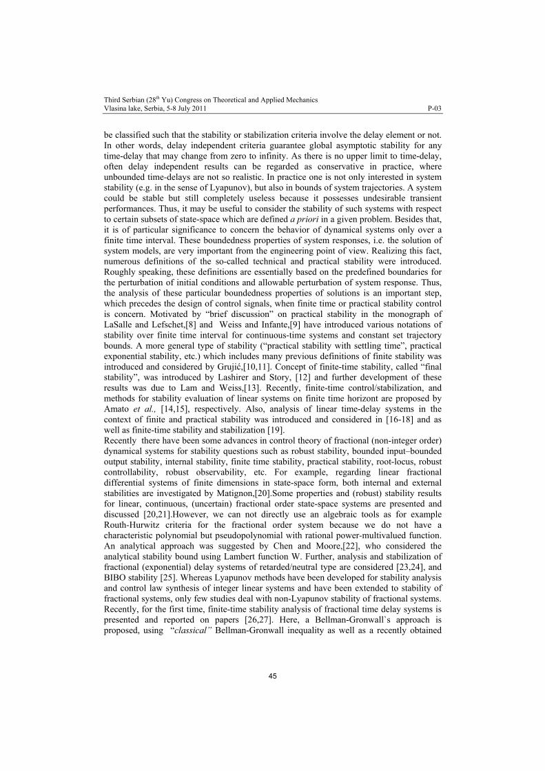
Third Serbian (28th Yu) Congress on Theoretical and Applied Mechanics Vlasina lake, Serbia, 5-8 July 2011 P-03
be classified such that the stability or stabilization criteria involve the delay element or not. In other words, delay independent criteria guarantee global asymptotic stability for any time-delay that may change from zero to infinity. As there is no upper limit to time-delay, often delay independent results can be regarded as conservative in practice, where unbounded time-delays are not so realistic. In practice one is not only interested in system stability (e.g. in the sense of Lyapunov), but also in bounds of system trajectories. A system could be stable but still completely useless because it possesses undesirable transient performances. Thus, it may be useful to consider the stability of such systems with respect to certain subsets of state-space which are defined a priori in a given problem. Besides that, it is of particular significance to concern the behavior of dynamical systems only over a finite time interval. These boundedness properties of system responses, i.e. the solution of system models, are very important from the engineering point of view. Realizing this fact, numerous definitions of the so-called technical and practical stability were introduced. Roughly speaking, these definitions are essentially based on the predefined boundaries for the perturbation of initial conditions and allowable perturbation of system response. Thus, the analysis of these particular boundedness properties of solutions is an important step, which precedes the design of control signals, when finite time or practical stability control is concern. Motivated by “brief discussion” on practical stability in the monograph of LaSalle and Lefschet,[8] and Weiss and Infante,[9] have introduced various notations of stability over finite time interval for continuous-time systems and constant set trajectory bounds. A more general type of stability (“practical stability with settling time”, practical exponential stability, etc.) which includes many previous definitions of finite stability was introduced and considered by Grujić,[10,11]. Concept of finite-time stability, called “final stability”, was introduced by Lashirer and Story, [12] and further development of these results was due to Lam and Weiss,[13]. Recently, finite-time control/stabilization, and methods for stability evaluation of linear systems on finite time horizont are proposed by Amato et al., [14,15], respectively. Also, analysis of linear time-delay systems in the context of finite and practical stability was introduced and considered in [16-18] and as well as finite-time stability and stabilization [19]. Recently there have been some advances in control theory of fractional (non-integer order) dynamical systems for stability questions such as robust stability, bounded input–bounded output stability, internal stability, finite time stability, practical stability, root-locus, robust controllability, robust observability, etc. For example, regarding linear fractional differential systems of finite dimensions in state-space form, both internal and external stabilities are investigated by Matignon,[20].Some properties and (robust) stability results for linear, continuous, (uncertain) fractional order state-space systems are presented and discussed [20,21].However, we can not directly use an algebraic tools as for example Routh-Hurwitz criteria for the fractional order system because we do not have a characteristic polynomial but pseudopolynomial with rational power-multivalued function. An analytical approach was suggested by Chen and Moore,[22], who considered the analytical stability bound using Lambert function W. Further, analysis and stabilization of fractional (exponential) delay systems of retarded/neutral type are considered [23,24], and BIBO stability [25]. Whereas Lyapunov methods have been developed for stability analysis and control law synthesis of integer linear systems and have been extended to stability of fractional systems, only few studies deal with non-Lyapunov stability of fractional systems. Recently, for the first time, finite-time stability analysis of fractional time delay systems is presented and reported on papers [26,27]. Here, a Bellman-Gronwall`s approach is proposed, using “classical” Bellman-Gronwall inequality as well as a recently obtained
45

Third Serbian (28th Yu) Congress on Theoretical and Applied Mechanics Vlasina lake, Serbia, 5-8 July 2011 P-03
generalized Gronwall inequality reported in [28] as a starting point. The problem of sufficient conditions that enable system trajectories to stay within the a priori given sets for the particular class of (non)linear (non)autonomous fractional order time-delay systems has been examined.
2. Fundamentals of fractional calculus
Fractional calculus (FC) as an extension of ordinary calculus has a 300 years old history. FC was initiated by Leibniz and L`Hospital as a result of a correspondence which lasted several months in 1695. Both Leibniz and L`Hospital, aware of ordinary calculus, raised the question of a noninteger differentiation (order 1/ 2n ) for simple functions. Subsequent mention of fractional derivatives was made, in some context or the other by (for example) Euler in 1730, Lagrange in 1772, Laplace in 1812, Lacroix in 1819, Fourier in 1822, Riemann in 1847, Green in 1859, Holmgren in 1865, Grunwald in 1867, Letnikov in 1868, Sonini in 1869, Laurent in 1884, Nekrassov in 1888, Krug in 1890, and Weyl in 1919, etc. [29]. In that way, the theory of fractional-order derivative was developed mainly in the 19th century. Since from 19th century as a foundation of fractional geometry and fractional dynamics, the theory of FO, in particular, the theory of FC and FDEs and researches of application have been developed rapidly in the world. The modern epoch started in 1974 when a consistent formalism of the fractional calculus has been developed by Oldham and Spanier,[4], and later Podlubny,[6]. Applications of FC are very wide nowadays, in rheology, viscoelasticity, acoustics, optics, chemical physics, robotics, control theory of dynamical systems, electrical engineering, bioengineering and so on, [4-12]. In fact, real world processes generally or most likely are fractional order systems. The main reason for the success of applications FC is that these new fractional-order models are more accurate than integer-order models, i.e. there are more degrees of freedom in the fractional order model. Furthermore, fractional derivatives provide an excellent instrument for the description of memory and hereditary properties of various materials and processes due to the existence of a ”memory” term in a model. This memory term insure the history and its impact to the present and future. A typical example of a non-integer (fractional) order system is the voltage-current relation of a semi-infinite lossy transmission line [17] or diffusion of the heat through a semi-infinite solid, where heat flow is equal to the half-derivative of the temperature [6].In his 700 pages long book on Calculus, 1819 Lacroix [30]
developed the formula for the n-th derivative of , m – is a positive integer, mxy
!
!n m m nm
D xm n
x
where is an integer. Replacing the factorial symbol by the
Gamma function, he further obtained the formula for the fractional derivative
n m
1
1D x x
(1)
where and are fractional numbers and Gamma function z is defined for 0z
by the so-called Euler integral of the second kind:
(2) 1
0
, ( 1) ( )x zz e x dx z z z
46

Third Serbian (28th Yu) Congress on Theoretical and Applied Mechanics Vlasina lake, Serbia, 5-8 July 2011 P-03
On the other hand, Liouville (1809-1882) formally extended the formula for the derivative of integral order n
. (3) ,n ax n ax ax axD e a e D e a e arbitrary order
Using the series expansion of a function, he derived the formula known as Liouville`s first formula for fractional derivative, where may be rational, irrational or complex.
(4) 0
( ) na xn n
n
D f x c a e
where . However, it can be only used for functions of the
previous form. Also, it was J. B. J. Fourier,[31] who derived the functional representation of function
0
exp( ), Re 0n n n
n
f x c a x a
1( ) cos
2R R
f t f x d d
, (5)
where he also formally introduced the fractional derivative version. In 1823, Abel considered a mechanical problem, namely Abel’s mechanical problem [32]. In the absence of friction, the problem is reduced to an integral equation
1/ 2
0
( ) 2 ( ), 0,y
y z u z dz g f y y H
, (6)
where 21 ( ) ,u z z z is an increasing function, g is the constant downward
acceleration, f y is a prescribed function. Then Abel solved (6) in [33]. Also an Abel
transform of a sufficiently well behaved function u was generalized to
1
1( ) ,
x
a
x t u t dt a x b
1
, (7)
where and , 0,a b (.) is the well known Euler's gamma function. Here,
it is assumed the solution of classical Abel integral equation exists and the fractional
derivative with order 1,0 exists in , [34], so we have following results: ),ba(1L
Lemma1.Consider, for ba,1,0 , the classical Abel integral equation
x
a
bxaxfdttutx ),()(1 1
, (8)
Then there exists at most one solution of equation (8) in . Moreover, if the
function is absolutely continuous on [a, b], then equation (8) has a solution in ,
given by (9)
),(1 baL
f ),(1 baL
47

Third Serbian (28th Yu) Congress on Theoretical and Applied Mechanics Vlasina lake, Serbia, 5-8 July 2011 P-03
x
a
bxaxfdttftxdx
dxu ),()(
1
1)(
, (9)
If and are finite, then a af
bxadttftxaxafxux
a
,,)(
1
1)(
, (10)
If is finite and is extended by 0 to the left of , then a f a
bxatdftxxux
a
,)(1
1)(
0
, (11)
If is finite and a 0)(lim 1 xfxx
then
bxtdftxxux
,)(1
1)(
, (12)
From the viewpoint of fractional calculus, we can see that (9)–(12) are just some other forms of fractional derivatives, with order 1,0 , under some different hypotheses on .
Fractional derivatives are typically treated as a particular case of pseudo-differential operators. Since they are nonlocal and have weakly singular kernels, the study of fractional differential equations seems to be more difficult and less theories have been established than for classical differential equations. In 1832-1837 a series of papers by Liouville [35,36] reported the earliest form of the fractional integral, though not quite rigorously from the mathematical point of view. The formula was taken as follows
f
0
1 0,,1
1)( pxdtttx
pxD p
pp , (13)
That is now called the Liouville form of fractional integral with the factor being
omitted. Next the significant work was done by Riemann [37], who wrote that paper in 1847 when he was just a student. But it was published until 1876, ten years after his death. Riemann had arrived at the expression
p1
10
1,RL D x d x
x
0 (14)
for fractional integration. Furthermore, we have the most useful forms of left-hand and right-hand Riemann- Liouville (RL) derivatives defined as follows
48

Third Serbian (28th Yu) Congress on Theoretical and Applied Mechanics Vlasina lake, Serbia, 5-8 July 2011 P-03
1
,
1
,
1,
1,
xmm
RL a x m
a
m bmm
RL x b m
x
dD f x x f d
m dx
dD f x x f d
m dx
(15)
where 1m m , a, b are the terminal points of the interval ,a b , which can also be
. The definition (15) of the fractional differentiation of Riemann-Liouville type leads a conflict between the well-established and polished mathematical theory and proper needs, such as the initial problem of the fractional differential equation, and the nonzero problem related to the Riemann-Liouville derivative of a constant, and so on. A certain solution to this conflict was proposed by Caputo first in his paper [38] (1967) .Caputo’s definitions can be written as
,
1
,
1
,
1,
1,
xm m
C a x
a
m bmm
C x b m
x
D f x x f dm
dD f x x f d
m dx
(16)
where . Obviously, the Caputo derivative is more strict than Riemann-Liouville derivative, one reason is that the m-th order derivative is required to exist. The Caputo and Riemann-Liouville formulation coincide when the initial conditions are zero. Besides, the RL derivative is meaningful under weaker smoothness requirements. Also, the RL derivative can be presented as:
1m m
, ( ), 1, ,n nRL x a xD f x D D f x n n (17)
and the Caputo derivative
, ,( ) ( ), 1, ,n nC a x a xD f x D D f x n n n (18)
where is the classical -order derivative. Moreover, previous expressions show that the fractional-order operators are global operators having a memory of all past events, making them adequate for modeling hereditary and memory effects in most materials and systems. Also, for the RL derivative, we have
nDZn , n
1
1
)1(
)()(lim
n
n
tRL
an dt
txdtxD
and
n
n
tRL
an dt
txdtxD
)()(lim
(19)
But for the Caputo derivative, we have
)()(
)(lim )1(1
1
)1(axD
dt
txdtxD n
n
n
tCa
n
and n
n
tCa
n dt
txdtxD
)()(lim
(20)
Obviously, varies continuously with , but the Caputo derivative
cannot do this. On the other side, initial conditions of fractional differential equations with Caputo derivative have a clear physical meaning and Caputo derivative is extensively used in real applications. On the other side, Grunwald [39] (in 1867) and Letnikov [40] (in 1868) developed an approach to fractional differentiation based on the definition
, ,RL aD n n
49

Third Serbian (28th Yu) Congress on Theoretical and Applied Mechanics Vlasina lake, Serbia, 5-8 July 2011 P-03
00
( ) lim , 1 , 0,h j
GL x hhj
f xD f x f x f x jh h
jh
(21)
which is the left Grunwald-Letnilov (GL) derivative as a limit of a fractional order backward difference. Similarly, we have the right one as
00
( ) lim , 1 , 0,h j
GL x hhj
f xD f x f x f x jh h
jh
(22)
Therefore, one can define the new form of Grunwald-Letnikov derivative as follows
0
1( ) lim ,
2cos2
h h
GL x h
f f xD f x
h
(23)
which is called the Grunwald-Letnikov-Riesz derivative. As indicated above, the previous definition of GL is valid for α > 0 (fractional derivative) and for α < 0 (fractional integral) and, commonly, these two notions are grouped into one single operator called differintegral. The GL derivative and RL derivative are equivalent if the functions they act on are sufficiently smooth. For numerical calculation of fractional–order differ-integral operator one can use relation derived from the GL definition.
(24)
0
N( x )
x j( x Lj
D f ( x ) h b f ( x jh )
where L is the "memory length", h is the step size of the calculation,
( ) , ,x L
N t minh h
(25)
x is the integer part of x and jb
is the binomial coefficient given by
0
11 1( ) ( )
jb , b bj
1j
(26)
For convenience, Laplace domain is usually used to describe the fractional integro-differential operation for solving engineering problems. The formula for the Laplace transform of the RL fractional derivative has the form:
1
10 0 0
00
nsx k k
RL ,x RL ,x xk
e D f ( x )dx s F( s ) s D f ( x )
(27)
Where for 0 (i.e., for the case of a fractional integral) the sum in the right-hand side must be omitted). Also, Laplace transform of the Caputo fractional derivative is:
1
1 ( )0
00
( ) ( ) (0), 1n
st k kt
k
e D f t dt s F s s f n
n (28)
which implies that all the initial values of the considered equation are presented by a set of only classical integer-order derivatives. Besides that, a geometric and physical interpretation of fractional integration and fractional differentiation can be found in Podlubny’s work [41].
50

Third Serbian (28th Yu) Congress on Theoretical and Applied Mechanics Vlasina lake, Serbia, 5-8 July 2011 P-03
3. Preliminaries on integer time-delay systems
A linear, multivariable time-delay system can be represented by differential equation:
0 1
( )( ) ( )
dx tA x t A x t
dt (29)
and with associated function of initial state:
( ) ( ), 0,xx t t t (30)
Equation (29) is referred to as homogenous state equation. Also, more general a linear, multivariable time-delay system can be represented by following differential equation:
0 1 0 1
( )( ) ( ) ( ) ( ),
dx tA x t A x t B u t B u t
dt (31)
and with associated function of initial state and control: ( ) ( ), 0,
( ) ( ),x
x
x t t t
u t t
(32)
Equation (31) is referred to as nonhomogenous or the unforced state equation, ( )x t is state
vector, control vector, ( )u t 0 1 0, ,A A B and are constant system matrices of appropriate
dimensions, and 1B
is pure time delay, =const. ( >0). Moreover, here it is considered a class of non-linear system with time delay described by the state space equation:
0 1 0 1
1 1
( )( ) ( ) ( ) ( ) ( ) ( ) ,
n m
i j
i j
d tA t A t B t B t f t f t
dt
xx x u u x x (33)
with the initial functions (32) of the system. Vector functions , , 1, , 1,i jf f i n j m
( )tx ( )t
present nonlinear parameter perturbations of system in respect to and x
respectively. Also, it is introduced next assumption that:
( , 1, 0,
( , 1, ,
i i
j j
f (t)) c (t) i n t
f (t - )) c (t - ) j m t
0, )
x x
x x (34)
where ,i jc c R are known real positive numbers. Moreover, a linear multivariable time-
varying delay system can be represented by differential equation
0 1 0( )
( ) ( ) ( ),dx t
A x t A x t t B u tdt
(35)
and with associated function of initial state ( ) ( ), 0.x Mx t t t (36)
where t is an unknown time–varying parameter which satisfies
0 , , , ,M o ot t J J t t T J R (37)
Moreover, here it is considered a class of perturbed non-linear system with time delay described by the state space equation
51

Third Serbian (28th Yu) Congress on Theoretical and Applied Mechanics Vlasina lake, Serbia, 5-8 July 2011 P-03
0 0 1 1 0 0( )
( ) ( ( )) ( ) ( ), ( ( )) ,dx t
A A x t A A x t t B u t f x t x t tdt
(38)
with the given initial functions of the system and vector function 0f .Vector function 0f
present nonlinear parameter perturbations of system in respect to ( )x t and ( ( ))x t t
respectively and matrices present perturbations of system, too. Also, it is
assumed that next assumption is true. 0 ,A A 1
0 0 1( ( ), ( ( ))) ( ) ( ( )) , 0, ,f x t x t - t c x t c x t - t t (39)
where are known real positive numbers. Dynamical behavior of system
(29),(31) or (33) with initial functions (30),or (32) is defined over time interval 0 1,c c R
t To o , J t , where quantity T may be either a positive real number or symbol + ,
so finite time stability and practical stability can be treated simultaneously. It is obvious that
J R . Time invariant sets, used as bounds of system trajectories, are assumed to be open, connected and bounded. Let index "" stands for the set of all allowable states of system and index for the set of all initial states of the system, such that the set
. In general, one may write:
""
SS
2: ( ) , ,
QS t x x , (40)
where Q will be assumed to be symmetric, positive definite, real matrix. u
S denotes the
set of the all allowable control actions. Let .x be any vector norm (e.g., ) and . 1,2,
(.) the matrix norm induced by this vector. Matrix measure has been widely used in the
literature when dealing with stability of time delay systems. The matrix measure for any
matrix is defined as follows: n nA C
0
1lim
I AA
(41)
The matrix measure defined in (36) can be subdefined in three different ways, depending on the norm utilized in its definitions,[42].
11
max Ren
kk ikk
ii k
A a
a , (42)
21
max Ren
kk ikk
ii k
A a
a , (43)
52

Third Serbian (28th Yu) Congress on Theoretical and Applied Mechanics Vlasina lake, Serbia, 5-8 July 2011 P-03
and 1
max Ren
ii kii
ii k
A a
a (44)
Expression (32) can be written in it’s general form as:
( ) ( ), 0, ( ) ,
( ) ( ), 0, ( ) , 0
o x x
o u u
t C
t C
x
u
0, (45)
where is the initial time of observation of the system (29) and ot ,0C -τ is a Banach
space of continuous functions over a time interval of length , mapping the interval
into R with the norm defined in the following manner:
τ
t,t n
0
max ( )C
, (46)
It is assumed that the usual smoothness condition is present so that is no difficulty with questions of existence, uniqueness, and continuity of solutions with respect to initial data. 3.1 Some previous results related to integer time-delay systems
The existing methods developed so far for stability check are mainly for integer-order systems. Definition 1: System given by (31) with 0,t - t u ,satisfying initial condition (4) is
finite stable w.r.t 0( ), , , , ,ut J 0 ,A if and only if:
,x S t , 0 (47)
and
,u
t S t J u (48)
imply: 0( ; , ) , 0,t t S t T 0x x (49)
Illustration of preceding definition is pictured on Fig. 1.
Fig.1 Finite time stability concept illustration
53
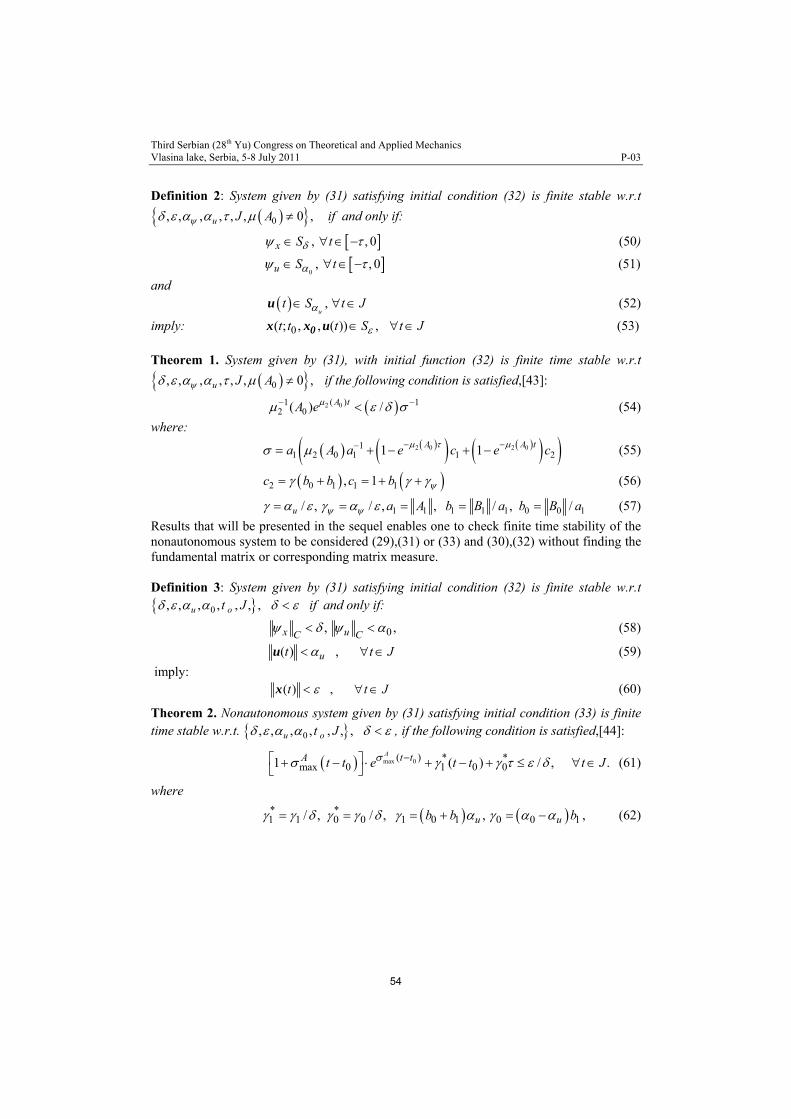
Third Serbian (28th Yu) Congress on Theoretical and Applied Mechanics Vlasina lake, Serbia, 5-8 July 2011 P-03
Definition 2: System given by (31) satisfying initial condition (32) is finite stable w.r.t
if and only if: 0, , , , , , 0 ,u J A
,x S t , 0 (50)
0, ,u S t 0 (51)
and (52) ,
ut S t J u
imply: 0( ; , , ( )) ,t t t S t J 0x x u (53)
Theorem 1. System given by (31), with initial function (32) is finite time stable w.r.t
if the following condition is satisfied,[43]: 0, , , , , , 0 ,u J A 2 0( )1 1
2 0( ) /A tA e (54)
where:
2 0 2 011 2 0 1 1 21 1A Aa A a e c e c t (55)
2 0 1 1 1, 1c b b c b (56)
1 1 1 1 1 0 0/ , / , , / , /u a A b B a b B a 1 (57)
Results that will be presented in the sequel enables one to check finite time stability of the nonautonomous system to be considered (29),(31) or (33) and (30),(32) without finding the fundamental matrix or corresponding matrix measure. Definition 3: System given by (31) satisfying initial condition (32) is finite stable w.r.t
0, , , , , , ,u ot J if and only if:
0,x uC C , (58)
( ) ,ut u t J (59)
imply: ( ) ,t t x J (60)
Theorem 2. Nonautonomous system given by (31) satisfying initial condition (33) is finite time stable w.r.t. 0, , , , , , ,u ot J , if the following condition is satisfied,[44]:
(61) max 0( ) * *max 0 1 0 01 ( )
A t tA t t e t t t J / , .
where
* *1 1 0 0 1 0 1 0 0/ , / , ,ub b b 1u , (62)
54

Third Serbian (28th Yu) Congress on Theoretical and Applied Mechanics Vlasina lake, Serbia, 5-8 July 2011 P-03
4. Preliminaries on stability of fractional order systems including time-delays
In the field of fractional-order control systems, there are many challenging and unsolved problems related to stability theory such as robust stability, bounded input – bounded output stability, internal stability, root-locus, robust controllability, robust observability, etc. In engineering, the fractional order is often less than 1, so we restrict as
usual. Even if
0,1
1 , we can translate the fractional systems into systems with the same
fractional order which lies in provided some suitable conditions are satisfied [45]. To
demonstrate the advantage of fractional calculus in characterizing system behavior,here, stability properties, let us consider the following illustrative example, [46].
0,1
Example 1: Compare the following two systems with initial condition (0)x for 0 1 ,
1 10,( ) , ( ) , 0 1.C t
dx t t D x t t
dt (63)
The analytical solutions of previous systems are and (0)t x
1( )(0)
tx
,
respectively. One may conclude, the integer-order system is unstable for any .
However, the second,given fractional dynamic system is stable as
0,1 0 1 , which
implies that fractional-order system may have additional attractive feature over the integer-order system. Also, in [47], Tarasov proposed that stability is connected to motion changes at fractional changes of variables where systems which are unstable “in sense of Lyapuov”' can be stable with respect to fractional variations. In 1996, Matignon [48] studied the following fractional differential system involving Caputo derivative
0, 0, (0) , 0,1C t
d xD Ax t x x
dt
(64)
where 1 2, ,...,T
n x x x x with initial value 0 10 20 0, ,..., ,T n n
nx x x x A R .The stability of
the equilibrium of system (64) was first defined and established by Matignon as follows. Definition 4. The autonomous fractional order system (64) is said to be
(a) stable iff for any 0x , there exists 0 such that (65)
x for 0t
(b) asymptotically stable iff lim 0t x t (66)
Also,Matignon [48] proposed definition of the BIBO stability for fractional differential system. Definition 5. An input/output linear fractional system (67)
0, (0)d x
Ax Bu x xdty Cx
(67)
,n px R y R is externally stable or bounded-input bounded-output (BIBO) iff
, , ,mR y h u L R R pu L R which is equivalent to: 1 , p mh L R R .
55

Third Serbian (28th Yu) Congress on Theoretical and Applied Mechanics Vlasina lake, Serbia, 5-8 July 2011 P-03
Also, in [49] authors give two definitions of the stability for differential systems with the Caputo derivative and Riemann-Liouville derivative, respectively. Besides, the asymptotical stability of higher-dimensional linear fractional differential systems with the Riemann-Liouville fractional order and Caputo fractional order were studied where the asymptotical stability theorems were also derived. Definition 6. The zero solution of the following differential system with the α-th order Caputo derivative in which 0 < α < 1
0,C tD X AX (68)
is said to be:
(i) Stable, if 0, 0, when 0X , the solution X t to (68) with the initial
condition 0X t X satisfies ( )X t for any . (69) 0t (ii) Asymptotically stable, if the zero solution to (68) is stable, and it is locally attractive,
i.e., there exists a 0 such that 0X 0 implies that
lim ( ) 0t
X t
(70)
Definition 7. The zero solution of the following differential system with the α-th order Riemann- Liouville derivative in which 0 < α < 1
0,RL tD X AX (71)
is said to be:
(i) Stable, if 0, 0, when 0X , the solution X t to (71) with the initial
condition satisfies 10, 0RL t t
D X t
0X
( )X t for any . (72) 0t (ii) Asymptotically stable, if the zero solution to (71) is stable, and it is locally attractive, i.e., there exists a 0 such that 0X 0 implies that
lim ( ) 0t
X t
(73)
Next, one may study the stability of fractional differential systems in two spatial dimensions, and then study the fractional differential systems with higher dimensions. Now, it is studied the fractional differential system with the Caputo derivative,
* 0, , 0,1 , n ntD X AX A R (74)
where fractional derivative * 0 . They studied the
fractional differential system with the Caputo derivative,as follows: , 0, 0,(..) (..) (..)t C t RL tD D or D
0, , 0,1 ,CtD X AX A R n n (75)
Theorem 3. If the real parts of all the eigenvalues of A are negative, then the zero solution to system (75) is asymptotically stable. Also for fractional differential system with the Riemann-Liouville derivative
0, , 0,1 ,RLtD X AX A R n n (76)
they stated following theorem. Theorem 4. If the real parts of all the eigenvalues of A are negative, then the zero solution to system (76) is asymptotically stable.
56

Third Serbian (28th Yu) Congress on Theoretical and Applied Mechanics Vlasina lake, Serbia, 5-8 July 2011 P-03
A fractional-order linear time invariant system can be represented in the following pseudostate space form:
( )( ) ( )
( ) ( )
d x tAx t Bu t
dty t Cx t
(77)
where the notation /d dt indicates the Caputo fractional derivative of fractional
commensurate order , ,n mx R u R and py Rn nA R
are pseudo-state, input, and output
vectors of the system, respectively, and , ,n m p nB R C R . It is worth mentioning that the state space form Eq. (77) is a pseudo-representation because the
knowledge of vector x at time 0t t and input vector u t 0t t
0t
for are not entirely
sufficient to know the behavior of system (77) for . A fractional-order model is in
fact infinite dimensional, therefore its true state vector should be also infinite dimensional.
t
Theorem 5[48]: The following autonomous system,(64)
0 0
( )( ), , 0 1
d x tAx t x t x
dt
(78)
nx R , and A is an matrix, is asymptotically stable if and only if n n / 2arg is
satisfied for all eigenvalues of matrix A. In this case, each component of the states
decays toward 0 such as t . Also, this system is stable if and only if / 2arg is
satisfied for all eigenvalues of matrix A with those critical eigenvalues satisfying
/ 2arg have geometric multiplicity of one.
Demonstration of this theorem is based on the computation of state vector of system
, 0, 0x t Nt t . response to non-zero initial conditions. However, this result
remains valid whatever the definition used given that for a linear system without delay, an autonomous system with non-zero initial conditions can be transformed into a non-autonomous system with null initial condition. Also, the stable and unstable regions for
10 is shown in Fig. 2 and they denote the stable and unstable regions for
10 by and , respectively. C
C
57

Third Serbian (28th Yu) Congress on Theoretical and Applied Mechanics Vlasina lake, Serbia, 5-8 July 2011 P-03
Fig. 2 Stability region of fractional-order linear time invariant system with order 0 1
For a minimal realization of (77), Matignon has also demonstrated the following theorem,[48]. Theorem 6. In [48], consider a system given by the following linear pseudostate space form with inner dimension n:
0
( )( ) ( ), (0)
( ) ( )
d x tAx t Bu t x x
dty t Cx t
(79)
where 0 1 . Also, assume that the triplet (A,B,C) is minimal. System (79) is bounded-
input bounded-output (BIBO) stable if and only if arg / 2 is satisfied for all
eigenvalues of matrix A. When system (79) is externally stable, each component of its
impulse response behaves like 1t at infinity. Exponential stability thus cannot be used to characterize asymptotic stability of fractional systems. A new definition is introduced.
Definition 8. t stability
Trajectory x(t) = 0 of system / ,d x t dt f t x t (unforced system) is t
asymptotically stable if the uniform asymptotic stability condition is met and if there is a positive real such that:
0 , ox t c Q x t such that 0 ,t t x t Qt (80)
t stability will thus be used to refer to the asymptotic stability of fractional systems.As
the components of the state x t slowly decay towards 0 following t , fractional
systems are sometimes called long memory systems.
5. Stability of fractional delay system
In spite of intensive researches, the stability of fractional order (time delay) systems remains an open problem. As for linear time invariant integer order systems, it is now well known that stability of a linear fractional order system depends on the location of the system poles in the complex plane. However, poles location analysis remains a difficult
58

Third Serbian (28th Yu) Congress on Theoretical and Applied Mechanics Vlasina lake, Serbia, 5-8 July 2011 P-03
task in the general case. For commensurate fractional order systems, powerful criteria have been proposed. The most well known is Matignon's stability theorem [48]. It permits us to check the system stability through the location in the complex plane of the dynamic matrix eigenvalues of the state space like system representation. Matignon's theorem is in fact the starting point of several results in the field. As we know, due to the presence of the exponential function se , this equation has an infinite number of roots, which makes the analytical stability analysis of a time-delay system extremely difficult. In the literature few theorems are available for stability testing of fractional-delay systems. Almost all of these theorems are based on the locations of the transfer function poles [24,50] and since there is no universally applicable analytical method for solving fractional-delay equations in s domain, the numerical approach is commonly used. In the field of infinite-dimensional fractional-delay systems most studies are concerned about the stability of a class of
distributed systems whose transfer functions involve s and/or se ,[51]. Many examples of fractional differential systems with delay can be found in the literature. Simple examples
such as ( ) exp( ) / , 0G s a s s a
G s
arising in theory of transmission lines [52], or one can
find in [53] fractional delay systems with transfer function of linked to the heat equation which leads to transfer functions such as ( )
cosh( )( ) , 0 1
sinh( )
x sG s x
s s or
2
2( )
(1 )
a s
a s
eG s
b e
(82)
For example, Hotzel [54] presented the stability conditions for fractional-delay systems
with the characteristic equation 0sas b cs d e
as
. Chen and Moore [22]
analyzed the stability of a class of fractional-delay systems whose characteristic function
can be represented as the product of factors of the form 0r csb e d where the
parameters ,and r are all real numbers. In fact, they computed the characteristic roots of the system using the Lambert W function, which has become a standard library function of many mathematical software. In other words, they got a stability condition of (83), given by a transcendent inequality via the Lambert function [22,55]. They considered the following delayed fractional equation
dcba ,,,
( )(
q
pq
d y tK y t
dt) (83)
where q and Kp are real numbers and 0 < q < 1, time delay τ is a positive constant and all the initial values are zeros. We are interested in telling whether the system (10) is stable or not for a given set of combination of the three parameters: q, Kp and τ. The stability condition is that for all possible q , r and Kp
1/0
qp
qW K
r
(84)
In inequality,W(.) denotes the Lambert function such that ( )( ) W xW x e x . However, such
a bound remains analytic and is difficult to use in practice. In paper [55], the application of Lambert W function to the stability analysis of time-delay systems is re-examined through actually constructing the root distributions of the derived a transcendental characteristic equation’s (TCE) of some chosen orders. It is found that the rightmost root of the original TCE is not necessarily a principal branch Lambert W function solution, and that a derived
59

Third Serbian (28th Yu) Congress on Theoretical and Applied Mechanics Vlasina lake, Serbia, 5-8 July 2011 P-03
TCE obtained by taking the nth power of the original TCE introduces superfluous roots to the system. Further, Matignon's theorem has been used in [56] to investigate fractional differential systems with multiple delays stability. The proposed stability conditions are based on the root locus of the system characteristic matrix determinant but the proposed conditions are thus difficult to use in practice. Authors used fractional derivative Caputo definition of derivative where by using the Laplace transform, it is introduced a characteristic equation for the above system with multiple time delays. They discovered that if all roots of the characteristic equation have negative parts, then the equilibrium of the above linear system with fractional order is Lyapunov globally asymptotical stable if the equilibrium exist that is almost the same as that of classical differential equations. Namely, the following n-dimensional linear fractional differential system with multiple time delays:
1
1
2
2
111 1 11 12 2 12 1 1
221 1 21 22 2 22 2 2
1 1 1 2 2 2
( )( ) ( ) ... ( ),
( )( ) ( ) ... (
..............
( )( ) ( ) ... (
n
n
q
n n nq
q
n n nq
qn
n n n n nn n nq
d x ta x t a x t a x t
d t
d x ta x t a x t a x t
d t
d x ta x t a x t a x t
d t
),
),n
(85)
where is real and lies in (0,1), the initial values iq ( ) ( )i ix t t are given for−
and , maxmax 0i j t ij 1, 2,...,i n . In this system, time-delay matrix
n n
ij R
n nT
, coefficient matrix ij n n
A a
, state variables , ,i i ijx t x t R
and initial values i t C 0 ,0m ax 0, ,ij
. Its fractional order is defined as
. If and ..., nq q q iq 1 2, ,q jq 1,2,i j ..., n , then system (85) is actually the
one considered in [56].
11 11 12
221 2 22
1 2
11 12 1
21 22 2
1 2
...
...
...
n
n
n n n
sq s sn
ss q sn
s s qn n nn
s a e a e a e
a e s a e a es
a e a e s a e
nns
(86)
where s denotes a characteristic matrix of system (1) and det s a characteristic
polynomial of (86). The distribution of det s ’s eigenvalues totally determines the
stability of system (86).
Theorem 7. If all the roots of the characteristic equation 0det s have negative
real parts, then the zero solution of system (1) is Lyapunov globally asymptotically stable. If n = 1, then (86) is reduced to the system studied in [56]. Bonnet and Partington [23,24] analyzes the BIBO stability of fractional exponential delay systems which are of retarded or neutral type. Conditions ensuring stability are given and these conditions can be expressed in terms of the location of the poles of the system. In view of constructing robust BIBO stabilizing controllers, explicit expressions of coprime and B´ezout factors of these systems are determined.Also,they have handled the robust
60

Third Serbian (28th Yu) Congress on Theoretical and Applied Mechanics Vlasina lake, Serbia, 5-8 July 2011 P-03
stabilization of fractional exponential delay systems of retarded type. The determination of coprime and B´ezout factors in the case of neutral systems is under study in both cases. However, all these contributions do not provide universally acceptable practical effective algebraic criteria or algorithms for testing the stability of a given general fractional delay system. Although the stability of the given general characteristic equation can be checked with the Nyquist criterion or the Mikhailov criterion, it becomes sufficiently difficult when a computer is used since one should find an angle of turn of the frequency response plot for an infinite variation of the frequency . A visual conclusion on stability with respect to the constructed part of the plot is not practically reliable, since, along with an infinite spiral, the delay generates loops whose number is infinite. As is evidenced from the literature the lack of universally acceptable algebraic algorithms for testing the stability of the characteristic equation has hindered the advance of control system design for fractional delay systems. This is particularly true in the case of designing fixed-structure fractional-order controller,
e.g., . On the other side, Hwang and Cheng [57] proposed a numerical algorithm which use methods that are based on the Cauchy integral theorem and suggested the modified complex integral in the form of
DPI
1 2 2( )
i
k ki
f sJ ds
s h ih f ih
(87)
where and are randomly chosen real constants lying in a specified interval and k
is a positive integer. The randomness of the parameters h1 and h2 makes the probability of the zero sum of the residues of all poles of the integrand being practically zero. Hence, the stability of a given fractional-delay system can be achieved by evaluating the integral
1 0h 2h
kJ and comparing its value with zero. Also, the proposed algorithm provides no idea about
the number and the location of unstable poles. In paper [58], an effective numerical algorithm for determining the location of poles and zeros on the first Riemann sheet is presented. The proposed method is based on the Rouche’s theorem and can be applied to all multi-valued transfer functions defined on a Riemann surface with finite number of Riemann sheets where the origin is a branch point. This covers all practical (finite-dimensional) fractional-order transfer functions and fractional-delay systems. 5.1 Finite time stability and stabilization of fractional order time delay systems As we know, the boundedness properties of system responses are very important from the engineering point of view. That is to say, enable system trajectories to stay within a priori given sets for the fractional order time-delay systems in state-space form, i.e., system stability from the non-Lyapunov point of view is considered. From this fact and our the best knowledge, we firstly introduced and defined finite-time stability for fractional order time delay systems [26-27, 60,62-63]. We also need the following definitions to analyze the case of fractional order systems with time-delay from non-Lyapunov point of view. First, we introduce the same order fractional differential system with time-delay (88) as well as multiple time delays (90) represented by the following differential equations:
* , 0 1 0
( )( ) ( ) ( ) ( ), 0 1,to t
d tD x t A t A t B u t
dt
x
x x (88)
with the associated function of initial state:
61
Third Serbian (28th Yu) Congress on Theoretical and Applied Mechanics Vlasina lake, Serbia, 5-8 July 2011 P-03
0( ) ( ) ,0 , 0xt t t C t x . (89)
Moreover, it is shown in [26] that fractional-order time delay state space model of PD control of Newcastle robot can be presented by (88) in state space form. Here, * , (.)to tD
denotes either Caputo fractional derivative , (.)C to tD or Riemann-Liouville fractional
derivative , (.)RL to tD . Also, fractional differential system with multiple time delays can be
presented as follows:
* , 0 0
1
1 2
( )( ) ( ) ( ) ( ), 0 1,
0 ... ...
n
to t i i
i
i m
d tD x t A t A t B u t
dt
xx x
(90)
with the associated function of initial state:
0( ) ( ) ,0 ,xx t t t C t 0. (91)
and where 0( 0,1,..., ),iA i m B are constant system matrices of appropriate dimensions, and
0 (i 1,2,..., )i m are pure time delays. Definition 9.[59] System given by (88), ( 0u t ) satisfying initial condition (89) is finite
stable w.r.t , , , , ,ot J if and only if:
,x C (92)
implies: ( ) , , x t t J (93)
Definition 10.[59] System given by (90), ( 0u t ) satisfying initial condition (91) is finite
stable w.r.t , , , , ,ot J if and only if:
,x C , , 0 t J J R , (94)
implies: ( ) , , x t t J (95)
Definition 11.[27,62]System given by (90) satisfying initial condition (91) is finite stable w.r.t , , , , , , ,u ot J if and only if:
, , ,0x Ct J J R (96)
and ( ) , , 0ut t J u u (97)
imply: ( ) ,t x t J (98)
Also, nonlinear fractional differential system with time delay in state and control can be presented as follows:
* , 0 1 0 1
1 1
( )( ) ( ) ( ) ( ) ( )
( ) ( ) , 0 1,
to t
n m
i j
i j
d tD x t A t A t B t B t
dt
f t f t
xx x u u
x x (99)
62

Third Serbian (28th Yu) Congress on Theoretical and Applied Mechanics Vlasina lake, Serbia, 5-8 July 2011 P-03
and with associated function of initial state and control:
( ) ( ), ( ) ( ), 0x ut t t t t x u (100)
Equation (99) is referred to as nonlinear nonhomogenous state equation, 0 1 0, ,A A B and
are constant system matrices of appropriate dimensions, and vector functions 1B
, , 1, , 1,i jf f i n j m
( )t
present nonlinear parameter perturbations of system in respect to
and ( )tx x respectively.
Definition 12: System given by (99) satisfying initial condition (100) is finite stable w.r.t
0, , , , , , ,u ot J if and only if:
0, ,x uC C (101)
( ) ,ut u t J (102)
imply: ( ) ,t x t J (103)
In what follows, we introduce the sufficient conditions on finite-time stability. In [59], we considered the fractional time-delay systems (88),(90) in the case of 0u t .
Theorem 8.(A) Autonomous system given by (88) satisfying initial condition (89) is finite time stable w.r.t. , , , , , ,ot J , if the following condition is satisfied:
max 0( )
1max 011
A t tA t te
/ , .t J (104)
where being the largest singular value of matrix (.), namely: (.)max
max max 0 max 1A A A , (105)
and is the Euler's gamma function. .
B) Autonomous system given by (90) satisfying initial condition (91) is finite time stable w.r.t. , , , , , ,ot J , if the following condition is satisfied:
( )
1max 0
0max
11
t tA
A
t te
/ , .t J (106)
where of matrices Amax i i
i
(.) A ,iA i = 0,1,2,...,n
n,...,2
. where being the
largest singular value of matrix
(.)max
iAi ,1,0, .
The above stability results for linear time-delay fractional differential systems were derived
by applying Bellman -Gronwall’s inequality. In that way, one can check system stability over finite time interval. Remark 1[60]: If 1 , case A, one can obtain same conditions which related to integer order time delay systems (1) as follows:
63

Third Serbian (28th Yu) Congress on Theoretical and Applied Mechanics Vlasina lake, Serbia, 5-8 July 2011 P-03
1
max 0( )1max 0 11 / ,
1
A t tA t te t J
, (2) 1 (107)
For the nonautonomous case,Zhang [61] also considered the following initial value problem
0, 0 1( ) ( ) ( ), 0; , ,0RL tD x t A x t A x t f t t x t t t (108)
where 0 < α < 1, is a given continuous function on [−τ, 0], 0A and 1A are constant
system matrices of appropriate dimensions, and is a constant with 0 . The system is defined over time interval 0,J T , where T is a positive number, f(t) is
a given continuous function on [0, T]. Similarly, the sufficient conditions of finite-time stability were derived by applying Bellman-Gronwall’s inequality. Theorem 9. System given by (108) satisfying initial condition is finite-time stable w.r.t 0, J, δ, ε, τ, δ <ε, if the following condition is satisfied:
( )
1 1max
/ , ,1
tAM t
e
t J (109)
Where /M f , and . is the Euler’s gamma function, 0sup
max max 0 max 1 1 max 1,A A A A . In paper [62], we considered a class of fractional non-linear perturbed autonomous system with time delay described by the state space equation:
0 0 1 1 0
( )( ) ( ) ( ) ,
d t A A t A A t f tdt
x
x x x (110)
with the initial functions (89)of the system and vector functions satisfied (34). 0f
Theorem 10. Nonlinear perturbed autonomous system given by (110) satisfying initial condition (89) and (34) is finite time stable w.r.t. , , , , , ot J , if the following
condition is satisfied:
0
0 1( )1 /
1
p t t
p t te , t J
1.
, (111)
where Euler's gamma function, and (.)0 10 1 1, ,Aoco Ao A A A Ac
1 1, ,p Aoco A Ao Ao A A
Remark 2: If we have no perturbed system 0 1 00, 0, ( (t)) 0 A A f x one can obtain
same conditions which related to Theorem 7. Further, paper [63] presents natural extension of the our paper [59] where it is obtained new stability criteria for nonautonomous fractional order time delay system (88). Theorem 11. Nonautonomous system given by (88) satisfying initial condition (89) is finite time stable w.r.t. 0, , , , , , ,u ot J , if the following condition is satisfied:
64

Third Serbian (28th Yu) Congress on Theoretical and Applied Mechanics Vlasina lake, Serbia, 5-8 July 2011 P-03
( )
1max 0 0
max 0 ( )1 /
1 1
t tAA
t t t te t
, .J (112)
where 0 0/ ,ub B 0b .
Remark 3. If 1 1B, one can obtain same conditions which related to integer order time
delay systems (31) , as follows, [18]: 0
1
max 0( )1 1max 0 01 ( )
1 /1 1
A t tA t t t te t
, , (2) 1J (113)
Moreover, in same paper [63], it is proposed finite time stability criteria for a class of fractional non-linear nonautonomous system with time delay in state and in control as follows:
0 1 0 1 0 1
( )( ) ( ) ( ) ( ) ( ) ( ) ,
d tA t A t B t B t f t f t
dt
x
x x u u x x (114)
with the initial functions (99) of the system and vector functions satisfied (34). 0 1,f f
Theorem 12: Nonlinear nonautonomous system given by (114) satisfying initial condition (99) is finite time stable w.r.t. 0, , , , , , ,u ot J , if the following condition is
satisfied: (115)
1 0 0 1 0 01max 01 0
0max 01( )1 / ,
1 1 1 1
t t
u uc
c t t t tt te t
J
b
where 0 0 1 1 01 0 1/ , / , /u u u ub b .
Recently, we studied and reported in paper,[27] finite-time stability analysis of linear fractional order single time delay systems where a Bellman-Gronwall`s approach is proposed, using as the starting point a recently obtained generalized Gronwall inequality reported in [28].
Theorem 13. The linear nonautonomous system given by (88) satisfying initial condition ( ) ( ), 0xx t t t is finite time stable w.r.t. 0, , , , ,u J , if the following
condition is satisfied:
max 01 0max 01 01 /
1 1ut t
E t t J
, 0,T , (116)
where 0 0 / ,u ub
max 01 max 0
and being the largest singular value of matrix (.),
where:
(.)max 1maxA A and .E denotes Mittag-Leffler function (see
Appendix). Remark 4. If 1
1B, one can obtain same conditions which related to integer order time
delay systems (31), as follows [18]: 0
65

Third Serbian (28th Yu) Congress on Theoretical and Applied Mechanics Vlasina lake, Serbia, 5-8 July 2011 P-03
1 ( ) 1max 0 01
1
1max 0 ( )
1 / ,1 1
( )
A t t
z
At t t t
e t
E z e
, (2) 1,J (117)
Theorem 14. The linear autonomous system given by Eq. (88) 0 0B , satisfying initial
condition ( ) ( ), 0xx t t t is finite time stable w.r.t. 0, , ,J , , if the
following condition is satisfied:
max 01max 01 01
1
tE t t
/ , J , (118)
Remark 5. In same manner, one may conclude that if 1 , see (21), it follows same conditions [60],Eq. (107) which relate to integer order time delay systems (29).
5.2 An illustrative example
Using a Time-Delay PD compensator on a linear system of equations with respect to the small perturbation , one may obtain: ( )e t y( ) ( )dt y t
( ) ( ) ( ) ( ) / ( ),P De t e t K e t K de t dt u t (119)
where: 1/ 2, 2, 3, 4,p DK K u
1 2( ) ( ), ( )
t -feedforward control. Also, all initial values
are zeros. Introducing: 1/ 2 1/ 2( ) /x t e t x t
( ) ,T
1 2t x xx
d e t dt ,one may write (119) in state-
space form, :
1 11/2
2 2
( ) ( )0 1 0 0 0( ) ( )
( ) ( )2 0 3 4 1tx t x t
D t u tx t x t
x , (120)
with an associated function of the initial state: ( ) ( ) 0, 0.xt t t x Now, we can
check the finite time stability wrt 0 0, 0,2 , 0.1, 100, 0.1, 1 ,ut J where
( ) 0, 0.1,0x t t . From the initial data and the Eq.(120) it yields:
max 0 max 1 max 0,1( ) 0.1, 2, 5, 7x Ct A A (121)
Applying the condition of the Theorem 13 (116) one can get:
0.5 0.5
0.50.5
7 101 7 100/ 0.1 0.1 .
0.886 0.886e e
e eT T
E T T
s (122)
eT being “estimated time” of finite time stability.
Conclusion In this paper, we have studied and presented the finite time stability of perturbed (non)linear fractional order time delay systems. We have employed the “classical” and the
66

Third Serbian (28th Yu) Congress on Theoretical and Applied Mechanics Vlasina lake, Serbia, 5-8 July 2011 P-03
generalization of Gronwall Belmann lemma to obtain finite time stability criteria for proposed class of time delay system. Also, they are presented some basic results on the stability of fractional order time delay systems as well as free delay systems. Finally, a numerical example is given to illustrate the validity of the proposed procedure. Acknowledgement. This work is partially supported by EUREKA program- E!4930 and the Ministry of Science and Environmental Protection of Republic of Serbia as Fundamental Research Project 41006 and 35006. Appendix Mittag-Leffler Function Similar to the exponential function frequently used in the solutions of integer-order systems, a function frequently used in the solutions of fractional-order systems is the Mittag-Leffler function defined as
0
,1
k
k
zE z
k
(A1)
where 0 and . The Mittag-Leffler function with two parameters appears most frequently and has the following form
z C
,
0
,k
k
zE z
k
(A2)
where 0, 0 , and . For z C 1 we obtain ,1E z E z and 1,1zE z e
Lemma (Gronwall Inequality). Suppose that ( )g t and are continuous in t 0 1, , 0, 0t t g t and are two
constants. If
0r
0
( )t
t g s s r ds (A3)
then 1 0 0 1
0
( ) exp ,
t
t r t t g s ds t t t A4)
Theorem A ([28] Generalized Gronwall inequality) Suppose ( ), ( )x t a t are nonnegative
and local integrable on ,and 0 ,t T some T ( )g t
con
is a nonnegative, nondecreasing
continuous function defined on 0 , (t T g t) M st , 0 with
1
0
( ) ( ) ( ) ( )
t
x t a t g t t s x s d s (A5)
on this interval.Then
1
10
( )( ) ( ) ( ) , 0
ntn
n
g tx t a t t s a s ds t T
n
(A6)
67

Third Serbian (28th Yu) Congress on Theoretical and Applied Mechanics Vlasina lake, Serbia, 5-8 July 2011 P-03
Corollary 2.1 of (Theorem A) [28] Under the hypothesis of Theorem 2.2, let be a
nondecreasing function on . Then holds:
( )a t
0,T
( ) ( )x t a t E g t t (A7)
References [1] Zavarei M., Jamshidi M.(1987),Time-Delay Systems: Analysis,Optimization and Applications,North-Holland,
Amsterdam. [2] Gorecki H., Fuksa, S., Grabowski, P., and Korytowski, A., (1989), Analysis and Synthesis of Time Delay
Systems, John Wiley and Sons, PWN-Polish Scientific Publishers-Warszawa. [3] Bellman, R.,Cooke, K. L., (1963), Differential-Difference Equations, Academic Press, New York. [4] Lee, T.N., Diant T.S.,(1981), Stability of Time Delay Systems, IEEE Trans. Automat. Cont. AC31(3) 951 953. [5] Mori,T.:,(1985),Criteria for Asymptotic Stability of Linear Time Delay Systems, IEEE Trans. Automat.
Control, AC-30, 158-161. [6] Hmamed,A.,(1986), On the Stability of Time Delay Systems: New Results, Int. J. Control 43, (1),321-324. [7] Chen,J., Xu,D., Shafai,B.,(1995), On Sufficient Conditions for Stability Independent of Delay, IEEE Trans.
Automat Control AC-40 (9) 1675-1680. [8] La Salle, Lefschet S.(1961), Stability by Lyapunov’s Direct Method,Academic Press, New York. [9] Weiss, L., F. Infante, (1965),On the Stability of Systems Defined over Finite Time Interval. Proc. National
Acad. Science 54(1). 44-48. [10] Grujić, Lj. T.,(1975a),Non-Lyapunov Stability Analysis of Large-Scale Systems on Time-Varying Sets. Int.
J. Control 21(3),401-405. [11] Grujić, Lj. T.,(1975b),Practical Stability with Settling Time on Composite Systems, Automatika, T.P. 9,1. [12] Lashirer, A. M., C. Story, (1972),Final-Stability with Applications, J. Inst. Math. Appl., 9, 379-410,1972. [13] Lam,L., L.Weiss,(1974),Finite Time Stability with Respect to Time-Varying Sets,J. Franklin Inst., 9,415-421. [14] Amato F., M. Ariola, and P. Dorato,(2001)Finite-time control of linear subject to parametric uncertainties and
disturbances,Automatica (IFAC),Vol. 37,pp. 1459-1463. [15] Amato F.,M. Ariola, and P. Dorato,(2007),Finite-time stabilization via dynamic output feedback, Automatica
(IFAC),Vol. 42, 337-342. [16] Debeljković, D. Lj, Lazarević M. P., Dj. Koruga, S. Tomašević,(1997),On Practical Stability of Time Delay
System Under Perturbing Forces,AMSE 97, Melbourne, Australia,October 29-31, 447-450. [17] Debeljković D. Lj., M. Lazarević, S. Milinković and M. Jovanović, (1998),Finite Time Stability Analysis of
Linear Time Delay System: Bellman-Gronwall Approach, IFAC International Workshop Linear Time Delay Systems, Grenoble,6-7 July,France, pp.171-176.
[18] Debeljković, Lj. D., Lazarević, M. P. et. a.,(2001),Further Results On Non-Lyapunov Stability of the Linear Nonautonomous Systems with Delayed State,Journal Facta Uversitatis,Vol.3,No 11,231-241,Niš, Serbia.
[19] Moulaya E.,M. Dambrineb,N. Yeganefarc,and W Perruquettic,(2008), Finite-time stability and stabilization of time-delay systems,Systems & Control Letters, 57, pp. 561–566.
[20] Matignon, D.,(1996),Stability result on fractional differential equations with applications to control processing. In IMACS - SMC Proceeding, July, Lille, France, 963- 968.
[21] Matignon,D.,(1998),Stability properties for generalized fractional differential systems, ESAIM: Proceedings, 5: 145 – 158, December.
[22] Chen, Y. Q., Moore K.L.,(2002), Analytical Stability Bound for a Class of Delayed Fractional-Order Dynamic Systems, Nonlinear Dynamics, Vol.29: 191-202.
[23] Bonnet C., J.R Partington,(2001)Stabilization of fractional exponential systems including delays,Kybernetika, 37,pp.345-353.
[24] Bonnet C., J.R Partington,(2002),Analysis of fractional delay systems of retarded and neutral type, Automatica, 38, pp.1133-1138.
[25] Hotzel, R., Fliess M.,(1998),On linear systems with a fractional derivation: Introductory theory and examples, Mathematics and Computers in Simulations,45 385-395.
[26] Lazarević,M., (2006),Finite time stability analysis of PD fractional control of robotic time-delay systems, Mechanics Research Communications,33, 269–279.
[27] Lazarević M., A.Spasić, (2009),Finite-Time Stability Analysis of Fractional Order Time Delay Systems: Gronwall`s Approach, Mathematical and Computer Modelling.
[28] H. Ye., J.Gao., Y. Ding.,(2007),A generalized Gronwall inequality and its application to a fractional differential equation, J. Math. Anal. Appl. 328 ,1075–1081.
[29] A.A. Kilbas, H.M. Srivastava, J.J. Trujillo, (2006),Theory and applications of Fractional Differential equations, edited by J.V. Mill (Elsevier, Amsterdam.
68

Third Serbian (28th Yu) Congress on Theoretical and Applied Mechanics Vlasina lake, Serbia, 5-8 July 2011 P-03
[30] Lacroix, S.F., (1819),Traite Du Calcul Differential et du Calcul Integral,2nd .Vol .3 Paris Courcier,409-410. [31] Fourier J. (1822),Théorie analytique de la chaleur. Paris. [32] R. Gorenflo, S. Vessella, (1991),Abel Integral Equations: Analysis and Applications, Lecture Notes in
Mathematics (Springer, Berlin Heidelberg). [33] N.H. Abel, Mag. (1823),Naturvidenskaberne 1, 11. [34] L. Tonelli, (1928),Su un problema di AbelAnna. Math. 99, 183. [35] Liouville, J.(1832),Memoire sur quelques questions e geometrie e de mecanique, et sur un noveaux genre de
calcul pour resoudre ces questions. J. l'Ecole Roy.Polytechn., 13, Sect. 21, 1-69. [36] Liouville, J. (1832),Memoire sur le calcul des dierentielles µa indice quelcon-ques. J. l'Ecole Roy. Polytechn.,
13, Sect. 21, 71-162. [37] B. Riemann, (1876),Gesamm. Math. Werke Wissensch. 331. [38] Caputo M., (1967),Linear models of dissipation whose Q is almost frequency independent. Part II. J Roy
Austral Soc. ;13:529-539. [39] A.K. Gr¨unwald,(1867), Z. Angew. Math. Phys. 12, 441. [40] A.V. Letnikov,(1868), Theory of differentiation offractional order,Mat. Sb. 3, 1. [41] Podlubny, I. (1999), Fractional Differential Equations, Academic Press, San Diego. [42] Desoer,C. A., M. Vidysagar,(1975),Feedback System:Input-Output Properties, Academic Press,New York . [43] Debeljković, D. Lj, Lazarević M. P., Dj. Koruga, S. Tomašević, (1997),On Practical Stability of Time Delay
System Under Perturbing Forces,AMSE 97, Melbourne, Australia,October 29-31, 447-450. [44] Debeljković, Lj. D., Lazarević M. P. et. al (2001), Further Results On Non-Lyapunov Stability of the Linear
Nonautonomous Systems with Delayed State, Journal Facta Uversitatis,Vol.3,No 11, 231-241, Niš, Serbia,Yugoslavia.
[45] C.P.Li and W.H. Deng ,(2007), Remarks on fractional derivatives, Applied Mathematics and Computation, 187, 777–784.
[46] Y. Li, Y.Quan Chen, I. Podlubny,(2010), Stability of fractional-order nonlinear dynamic systems: Lyapunov direct method and generalized Mittag_Leffler stability, Computers and Mathematics with Applications, 59. pp. 1810-1821.
[47] V.E. Tarasov,(2007), Fractional stability, arXiv.org>physics> http://arxiv.org/abs/0711.2117. [48] Matignon, D., (1996)Stability Results for Fractional Differential Equations With Applications to Control
Processing, Computational Engineering in Systems and Application Multi-Conference, IMACS, IEEE-SMC Proceedings, Lille, France, Vol. 2, pp. 963–968.
[49] LI Chang-pin , Zhao Zhen-gang ,(2009),Asymptotical stability analysis of linear fractional differential systems, J Shanghai Univ (Engl Ed), 13(3): 197–206
[50] D. Matignon,(1994), Repr´esentations en variables d’´etat de mod`eles de guides d’ondes avec d´erivation fractionnaire. Th`ese de doctorat, Univ. Paris XI,.
[51] Ozturk N, Uraz A.(1985), An analytic stability test for a certain class of distributed parameter systems with delay, IEEE Transactions on CAS ,32(4):393-39.
[52] Weber E,(1956), Linear Transient Analysis. Volume II. Wiley, New York . [53] Loiseau J. and H. Mounier,(1998), Stabilisation de l’´equation de la chaleur command´ee en flux. Syst`emes
Diff´erentiels Fractionnaires, Mod`eles, Methodes et Applications.ESAIM Proceedings 5 , 131–144. [54] Hotzel R.(1998), Some stability conditions for fractional delay systems. Journal of Mathematical Systems,
Estimation, and Control,8(4):1-19. [55] Chyi Hwang and Yi-Cheng Cheng, (2005),Use of Lambert W Function to Stability Analysis of Time-Delay
Systems, ACC2005. June 8-10, 2005. Portland, OR, USA,pp 4283-4288. [56] Deng W, C. Li, J. Lu,(2007), Stability analysis of linear fractional differential system with multiple time
delay, Nonlinear Dynamics 48, 409-416. [57] Hwang C, Cheng Y-C, (2006) A numerical algorithm for stability testing of fractional delay systems.
Automatica 42:825–831 [58] Farshad Merrikh-Bayat, (2007),New Trends in Nanotechnology and Fractional Calculus
Applications,chapter , Stability of Fractional-Delay Systems:A Practical Approach,pp 163-170. [59] Lazarević M., D.Debeljković,(2005),Finite Time Stability Analysis of Linear Autonomous Fractional Order
Systems with Delayed State,Asian Journal of Control,Vol.7, No.4. [60] Lazarević M, Debeljković,Lj.D., Nenadić,Z.Lj. and Milinković,SA,(2000), Finite Time Stability of Time
Delay Systems, IMA Journal of Math. Cont. and Inf. 17, 101-109. [61] ZhangX.,(2008),Some results of linear fractional order time-delay system,Appl. Math. Comput.197, 407-411. [62] Lazarević M., D. Debeljković,(2008), Robust Finite Time Stability of Nonlinear Fractional Order Time Delay
Systems, International Journal of Information and Systems Sciences,Vol.4.No.2, pp.301-315. [63] Lazarević P. M.(2007), On finite time stability of nonautonomous fractional order time delay systems, Int.
Journal: Problems of Nonlinear Analysis in Engineering Systems, 1(27),pp.123-148.
69
Third Serbian(28th Yu) Congress on Theoretical and Applied MechanicsVlasina lake, Serbia, 5-8 July 2011 P-04
INTERA CTION OF EIGENVALUES WITHAPPLICATIONS IN MECHANICS AND PHYSICS
Alexander P. SeyranianInstitute of MechanicsLomonosov Moscow State UniversityRussiae-mail:[email protected]
Abstract. This is a review paper presenting a general theory of interaction of eigenvaluesof complex matrices of an arbitrary dimension depending on real parameters. The cases ofweak and strong interaction are distinguished and their geometric interpretation in two andthree-dimensional spaces is given. General asymptotic formulae for eigenvalue surfaces neardiabolic and exceptional points are presented demonstrating crossing and avoided crossingscenarios. A physical example on propagation of light in a homogeneous non-magnetic crystalillustrates effectiveness and accuracy of the presented theory. As applications in mechanicsstability problems for a pendulum with periodically varying length and stabilization effect fora buckled elastic rod by longitudinal vibrations are considered.
Keywords: Coupling of eigenvalues, stability problems, physics, mechanics.
1. Introduction
The behavior of eigenvalues of matrices and differential operators dependent on parameters isa problem of general interest having many important applications in natural and engineeringsciences. In modern physics, e.g. quantum mechanics, crystal optics, physical chemistry,acoustics and mechanics, singular points of matrix spectra associated with specific effectshave attracted great interest of researchers since the papers [15] and [14]. These are the pointswhere matrices possess multiple eigenvalues. In applications the case of double eigenvaluesis the most important. With a change of parameters, coupling and decoupling of eigenvalueswith crossing and avoided crossing scenarios occur. In recent papers two important casesare distinguished: the diabolic points (DPs) and the exceptional points (EPs). From themathematical point of view DP is a point where the eigenvalues coalesce (become double),while corresponding eigenvectors remain different (linearly independent); and EP is a pointwhere both eigenvalues and eigenvectors merge forming a Jordan block. Both the DP andEP cases are interesting in applications and were observed in experiments. In early studiesonly real and Hermitian matrices were considered while modern physical systems require thestudy of complex symmetric and non-symmetric matrices.
In this paper we present the results on interaction of eigenvalues of complex matrices ofarbitrary dimension smoothly depending on multiple real parameters. Two essential cases ofweak and strong coupling based on a Jordan form of the system matrix are distinguished.These two cases correspond to diabolic and exceptional points, respectively. We derivegeneral formulae describing coupling and decoupling of eigenvalues, crossing and avoided
70

crossingof eigenvalue surfaces. We present typical (generic) pictures showing the movementof eigenvalues, the eigenvalue surfaces and their cross-sections. It is emphasized that thetheory of coupling of eigenvalues of complex matrices gives not only qualitative, but alsoquantitative results on the behavior of eigenvalues based only on the information taken at thesingular points.
Interaction of eigenvalues for real matrices depending on multiple parameters withmechanical applications is given in the book [10] where significant mechanical effects relatedto diabolic and exceptional points were studied. These include transference of instabilitybetween eigenvalue branches, bimodal solutions in optimal structures under stabilityconstraints, flutter and divergence instabilities in undamped nonconservative systems, effectof gyroscopic stabilization, destabilization of a nonconservative system by infinitely smalldamping, which were described and explained from the point of view of coupling ofeigenvalues. The presented theory for complex matrices is based on the papers [9, 4].
The paper is organized as follows. In section 2 we present general results on weak andstrong interaction of eigenvalues of complex matrices depending on parameters. These twocases correspond to the study of eigenvalue behavior near diabolic and exceptional points.Section 3 is devoted to a physical example of propagation of light in a homogeneous non-magnetic crystal. Section 4 presents applications in mechanics, and the conclusion is givenin section 5.
2. Interaction of Eigenvalues
Let us consider the eigenvalue problem
Au = λu (1)
for a generalm×m complex matrix A smoothly depending on a vector ofn real parametersp = (p1, . . . , pn). Assume that, atp = p0, the eigenvalue coupling occurs, i.e., the matrixA0 = A(p0) has an eigenvalueλ0 of multiplicity 2 as a root of the characteristic equationdet(A0 − λ0I) = 0; I is the identity matrix. This double eigenvalue can have one ortwo linearly independent eigenvectorsu, which determine the geometric multiplicity. Theeigenvalue problem adjoint to (1) is
A∗v = ηv, (2)
whereA∗ = AT
is theadjointmatrix operator (Hermitian transpose). The eigenvaluesλ andη of problems (1) and (2) are complex conjugate:η = λ .
Double eigenvalues appear at sets in parameter space, whose codimensions dependon the matrix type and the degeneracy (EP or DP). In this paper we analyze general(nonsymmetric) complex matrices. The EP degeneracy is the most typical for this typeof matrices. In comparison with EP, the DP degeneracy is a rare phenomenon in systemsdescribed by general complex matrices. However, some nongeneric situations may beinteresting from the physical point of view. As an example, we mention complex non-Hermitian perturbations of symmetric two-parameter real matrices, when the eigenvaluesurfaces have coffee-filter singularity.
71

Let us considera smooth perturbation of parameters in the formp = p(ε), wherep(0) = p0 andε is a small real number. For the perturbed matrixA = A(p(ε)), we have
A = A0 + εA1 + 12ε2A2 +o(ε2),
A0 = A(p0), A1 =n
∑i=1
∂A∂ pi
dpi
dε,
A2 =n
∑i=1
∂A∂ pi
d2pi
dε2 +n
∑i, j=1
∂ 2A∂ pi∂ p j
dpi
dεdpj
dε.
(3)
The double eigenvalue λ0 generally splits intoa pair of simple eigenvalues under theperturbation. Asymptotic formulae for these eigenvalues and corresponding eigenvectorscontain integer or fractional powers ofε.
2.1. WeakInteraction of Eigenvalues
Let usconsiderthe interaction of eigenvalues in the case ofλ0 with two linearly independenteigenvectorsu1 andu2. This interaction point is known as a diabolic point. Let us denoteby v1 andv2 two eigenvectors of the complex conjugate eigenvalueη = λ for the adjointeigenvalue problem (2) satisfying the normalization conditions
(u1,v1) = (u2,v2) = 1,
(u1,v2) = (u2,v1) = 0,(4)
where (u,v) = ∑ni=1uivi denotesthe Hermitian inner product. Conditions (4) define the
unique vectorsv1 andv2 for givenu1 andu2.For nonzero smallε, the two eigenvaluesλ+ andλ− resulting from thebifurcation ofλ0
and the correspondingeigenvectorsu± are given by
λ± = λ0 + µ±ε +o(ε),
u± = α±u1 +β±u2 +o(1).(5)
Thecoefficientsµ±, α±, andβ± are found from the 2×2 eigenvalue problem, see e.g. [10](
(A1u1,v1) (A1u2,v1)(A1u1,v2) (A1u2,v2)
)(α±β±
)= µ±
(α±β±
). (6)
Solvingthecharacteristicequation for (6), we find
µ± =(A1u1,v1)+(A1u2,v2)
2±
√D2 +(A1u1,v2)(A1u2,v1),
D = 12((A1u1,v1)−(A1u2,v2)).
(7)
We note that for Hermitian matricesA one can takev1 = u1 and v2 = u2 in (6), wherethe eigenvectorsu1 andu2 are chosen satisfying the conditions(u1,u1) = (u2,u2) = 1 and(u1,u2) = 0, and obtain the well-known formula.
72

Figure1. Eigenvalue interaction: (a) weak, (b) strong.
As the parameter vector passes the interaction pointp0 along the curvep(ε) in parameterspace, theeigenvaluesλ+ andλ− change smoothly and cross each other atλ0, see Figure 1a.At the same time, the corresponding eigenvectorsu+ and u− remain different (linearlyindependent) at all values ofε including the pointp0. We call this interactionweak. Bymeans of eigenvectors, the eigenvaluesλ± are well distinguished during the weak interaction.
We emphasizethat despite the eigenvaluesλ± and the eigenvectorsu± dependsmoothlyona single parameterε, they are non-differentiable functions of multiple parameters atp0 inthe senseof Frechét.
2.2. Strong Interaction of Eigenvalues
Let us considerinteraction of eigenvalues atp0 with a double eigenvalueλ0 possessing asingle eigenvectoru0. This case corresponds to the exceptional point. The second vector ofthe invariant subspace corresponding toλ0 is called an associated vectoru1 (also calledageneralized eigenvector; it is determined by the equation
A0u1 = λ0u1 +u0. (8)
An eigenvectorv0 and an associated vectorv1 of the matrixA∗ are determined by
A∗0v0 = λ 0v0, A∗
0v1 = λ 0v1 +v0,
(u1,v0) = 1, (u1,v1) = 0,(9)
wherethelasttwo equations are the normalization conditions determiningv0 andv1 uniquelyfor a givenu1.
Bifurcation of λ0 into two eigenvaluesλ± and the corresponding eigenvectorsu± aredescribedby, see [10]
λ± = λ0±√µ1ε + µ2ε +o(ε),
u± = u0±u1√µ1ε
+(µ1u0 + µ2u1−G−1A1u0)ε +o(ε),
(10)
whereG = A0−λ0I +u1v∗1. The coefficientsµ1 andµ2 are
µ1 = (A1u0,v0),
µ2 =((A1u0,v1)+(A1u1,v0)
)/2.
(11)
73

With a change ofε from negative to positive values, the two eigenvaluesλ± approach,collide with infinite speed (derivative with respect toε tends to infinity) atλ0, and divergein theperpendicular direction, see Figure 1b. The eigenvectors interact too. Atε = 0, theymergeto u0 up to a scalar complex factor. At nonzeroε, the eigenvectorsu± differ from u0
by the leading term±u1√µ1ε . This term takes the purely imaginary factori asε changes the
sign, forexample altering from negative to positive values.We call such an interaction of eigenvalues asstrong. An exciting feature of the strong
interaction is that the two eigenvalues cannot be distinguished after the interaction. Indeed,there is no natural rule telling how the eigenvalues before interaction correspond to thoseafter the interaction.
3. Applications in Physics
As a physical example, we consider propagation of light in a homogeneous non-magneticcrystal in the general case when the crystal possesses natural optical activity (chirality)and dichroism (absorption) in addition to biaxial birefringence, see [2] for the generalformulation. The optical properties of the crystal are characterized by the inverse dielectrictensorηηη . The vectors of electric fieldE and displacementD arerelated asE = ηηηD [5]. Thetensorηηη is described by a non-Hermitian complex matrix. The electric fieldE and magneticfield H in the crystal are determined by Maxwell’s equations
rotE =−1c
∂H∂ t
, rotH =1c
∂D∂ t
, (12)
wheret is timeandc is the speed of light in vacuum.A monochromatic plane wave of frequencyω that propagates in a direction specified by
a realunit vectors= (s1,s2,s3) has the form
D(r , t) = D(s)expiω(
n(s)c sT r − t
)
H(r, t) = H(s)expiω(
n(s)c sT r − t
),
(13)
wheren(s) is a refractive index, andr = (x1,x2,x3) is the real vector of spatial coordinates.Substituting the wave (13) into Maxwell’s equations (12), we find
H = n[s,ηηηD], D =−n[s,H], (14)
wheresquarebrackets indicate cross product of vectors [5]. Then we obtain an eigenvalueproblem for the complex non-Hermitian matrixA(s) dependent on the vector of parameterss= (s1,s2,s3):
Au = λu, A(s) = (I −ssT)ηηη(s), (15)
whereλ−2, u = D, andI is theidentity matrix. Multiplying the matrixA by the vectors fromthe left we conclude thatsTA = 0, i.e., the vectors is the left eigenvector with the eigenvalueλ = 0. Zero eigenvalue always exists, because det(I−ssT)≡ 0, if ‖s‖= 1.
The matrix A(s) defined by equation (15) is a product of the matrixI − ssT and theinverse dielectric tensorηηη(s). The symmetric part ofηηη constitutes the anisotropy tensordescribing the birefringence of the crystal. It is represented by the complex symmetricmatrixU, which is independent of the vector of parameterss. The antisymmetric part ofηηη is
74

determinedby theoptical activity vectorg(s) = (g1,g2,g3), describing the chirality (opticalactivity) of the crystal. It is represented by the skew-symmetric matrix
G = i
0 −g3 g2
g3 0 −g1
−g2 g1 0
. (16)
The vectorg is given by the expressiong(s) = γγγs, whereγγγ is the optical activity tensorrepresented bya symmetric complex matrix. Thus, the matrixG(s) depends linearly on theparameterss1, s2, s3.
In the presentformulation, the problem was studied in [2]. Below we present a specificnumerical example in case of a non-diagonal matrixγγγ, for which the structure of singularitieswasnot fully investigated. Unlike [2], where the reduction to two dimensions was carriedout, we work with the three-dimensional form of problem (15). Our intention here is to giveguidelines for using our theory by means of the relatively simple 3×3 matrix family, keepingin mind that the main area of applications would be higher dimensional problems.
For numericalexample, we choose the inverse dielectric tensor in the form
ηηη =
3 0 00 1 00 0 2
+ i
0 1 21 0 02 0 0
+ i
0 −s1 0s1 0 −s3
0 s3 0
(17)
wheres3 =√
1−s21−s2
2. The crystaldefined by (17) is dichroic and optically active withthe non-diagonal matrixγγγ. Whens1 = 0 ands2 = 0 the spectrum of the matrixA consistsof the double eigenvalueλ0 = 2 and the simplezero eigenvalue. The double eigenvaluepossesses the eigenvectorsu0, v0, and associated vectorsu1, v1. Calculating the derivativesof the matrixA(s1,s2) at the points0 = (0,0,1) and substituting it together with the vectorsof Jordan chainsu0, u1 andv0, v1 yields the vectorsf, g andh, r as
f = (0,4), g = (−4,0), h = (0,0), r = (−4,0). (18)
With these vectors we find from the approximations of the eigensurfaces Reλ (s1,s2) andImλ (s1,s2) in the vicinity of the points0 = (0,0,1):
Reλ± = 2±√
2s2 +2√
s21 +s2
2,
Imλ± =−2s1±√−2s2 +2
√s21 +s2
2.
(19)
Calculation of the exact solution of the characteristic equation for the matrixA withthe inverse dielectric tensorηηη defined by equation (17) shows a good agreement of theapproximations (19)with the numerical solution, see Figure 2. One can see that the bothsurfaces of real and imaginary parts have a Whitney umbrella singularity at the interactionpoint; the surfaces self-intersect along different rays, which together constitute a straight linewhen projected on parameter plane. Other physical examples related to strong and weakinteraction of eigenvalues are presented in [9, 4, 6].
75

Figure2. Eigensurfaces of a crystal and their approximations
4. Mechanical Applications
In this section we consider applications in mechanics. First we study oscillations and stabilityproblems for a pendulum with periodically varying length. It is a model of child’s swing.Then we consider stabilization effect for an elastic rod, compressed by a longitudinal forcegreater than the critical Euler’s value, by longitudinal vibrations applied to the rod end. Thisis called Chelomei’s problem.
4.1. Stability of a Pendulum with Variable Length
Oscillations of a pendulum with variable length is among classical problems of mechanics.Usually, the pendulum with periodically varying length is associated with a child’s swing.As probably everyone can remember, to swing a swing one must crouch when passingthrough the middle vertical position and straighten up at the extreme positions, i.e. performoscillations with a frequency which is approximately twice the natural frequency of the swing.Despite popularity of the swing, in the literature on oscillations and stability there are notmany analytical and numerical results on behavior of the pendulum with periodically varyinglength dependent on parameters. In this paper the stability of the lower vertical position ofthe pendulum with damping and arbitrary periodic excitation function is investigated.
Equation for motion of the swing can be derived with the use of angular momentumalteration theorem. Taking into account also linear damping forces we obtain
ddt
(ml2
dθdt
)+ γ l2 dθ
dt+mglsinθ = 0, (20)
wherem is themass,l is the length,θ is the angle of the pendulum deviation from the verticalposition,g is theacceleration due to gravity, andt is the time, Fig. 3.
It is assumedthat the length of the pendulum changes according to the periodic law
l = l0 +aϕ(Ωt),∫ 2π
0ϕ(τ)dτ = 0, (21)
where l0 is the meanpendulum length,a and Ω are the amplitude and frequency of theexcitation,ϕ(τ) is the smooth 2π-periodic function with zero mean value.
76

Figure3. Schemesof the pendulum with periodically varying length.
Figure4. Stabilizationregion in Chelomei’s problem
We introduce the following dimensionless parameters and variables
τ = Ωt, ε =al0
, Ω0 =√
gl0
, ω =Ω0
Ω, β =
γmΩ0
. (22)
Then,equation(20)can be written in the following form
θ +(
2εϕ(τ)1+ εϕ(τ)
+βω)
θ +ω2sinθ
1+ εϕ(τ)= 0 (23)
Here the dotdenotes differentiation with respect to new timeτ. Behavior of the systemgoverned by equation (23) will be studied in the following sections via analytical andnumerical techniques depending on three dimensionless problem parameters: the excitationamplitudeε, the damping coefficientβ , and the frequencyω under the assumptionε ¿ 1,β ¿ 1. It is convenient to change the variable by the substitutionq = θ(1+ εϕ(τ)). Withthis substitutionwe obtain a nonlinear equation forq which is useful for stability study of thevertical position of the pendulum as well as analysis of small oscillations. Equation (23) isused for stability and dynamics study of the pendulum with variable length. It is shown thatthe instability (parametric resonance) regions are semi-cones in three-dimensional parameterspace with singularities at the DP, see also [7, 1].
77

4.2. Chelomei’sproblem
The possibility to increase the stability of elastic systems by means of vibrations wasoriginally pointed out in [3]. In particular, he arrived at the conclusion that an elastic rodcompressed by a longitudinal force greater than the critical Euler’s value can be stabilized byhigh-frequency longitudinal vibrations applied to the rod end. In this study, formulas for theupper and lower critical frequencies of rod stabilization are derived and analyzed. It is shownthat, in contrast to the case of high-frequency stabilization of an inverted pendulum with avibrating suspension point, the rod is stabilized at excitation frequencies of the order of thenatural frequency of transverse oscillations belonging to a certain region.
We consider a straight elastic rod of constant cross section, loaded by a periodiclongitudinal forceP(t) = P0 + Ptφ(ωt) applied to itsend. The equation of transverseoscillations of the rod can be written as
m∂ 2u∂ t2 + γ
∂u∂ t
+P(t)∂ 2u∂x2 +EJ
∂ 4u∂x4 = 0, (24)
wherex is the coordinatealong the rod axis;t is the time;u(x, t) is the rod deflection function;m is the mass per unit length;EJ is the flexural rigidity;γ is the damping coefficient;Pt andω are the excitation amplitude and frequency of the longitudinal vibration, respectively. It isconvenient to introduce non-dimensional parametersε = Pt/P1 andα = P0/P1−1 whereP1
is the firstEuler buckling load. The simply supported ends of the rod are considered. Fig.4 presents the stabilization region in Chelomei’s problem. The singularities related to thepoints DP and EP are discussed, see also [13, 12].
5. Conclusion
We have discussed interaction of eigenvalues of systems smoothly depending on multiple realparameters. Diabolic and exceptional points have been mathematically described and generalformulae for interaction of eigenvalues at these points have been derived. This theory has avery broad field of applications since any physical or mechanical system contains parameters.Last applications of the interaction theory of eigenvalues are presented in [8, 11].
References
[1] Belyakov, A.O., Seyranian, A.P. and Luongo, A. (2009) Dynamics of the pendulum with periodically varyinglength.Physica D,238, pp. 1589–1597.
[2] Berry, M. V. and Dennis, M. R. (2003) The optical singularities of birefringent dichroic chiral crystals.Proc.R. Soc. Lond. A, 459, pp. 1261–1292.
[3] Chelomei, V.N. (1956) On possibility to increase stability of elastic systems by vibration.Doklady Akad. NaukSSSR, 110(3), pp. 345-347.
[4] Kirillov, O. N., Mailybaev, A. A. and Seyranian, A. P. (2005) Unfolding of eigenvalue surfaces near a diabolicpoint due to a complex perturbation.J. Phys. A: Math. Gen., 38, pp. 5531–5546.
[5] Landau, L. D., Lifshitz, E. M. and Pitaevskii, L. P. (1984)Electrodynamics of continuous media. Pergamon.Oxford.
[6] Mailybaev, A. A., Kirillov, O. N. and Seyranian, A. P. (2005), Physiscal Review A, 72, (014104), pp. 1–4[7] Seyranian, A. P. (2004) The swing: parametric resonance.Journal of Applied Mathematics and Mechanics,
68(5), pp. 757–764.[8] Seyranian, A.P. and Belyakov, A.O. (2011). How to twirl a hula hoop.American Journal of Physics(to appear).[9] Seyranian, A. P., Kirillov, O. N. and Mailybaev, A. A. (2005) Coupling of eigenvalues of complex matrices at
diabolic and exceptional points.J. Phys. A: Math. Gen., 38, pp. 1723U-1740.
78

[10] Seyranian,A. P. and Mailybaev, A. A. (2003)Multiparameter Stability Theory with Mechanical Applications.World Scientific. New Jersey.
[11] Seyranian, A.P. and Mailybaev, A.A. (2011). Paradox of Nicolai and related effects.ZAMP(to appear).[12] Seyranian, A.A. and Seyranian, A.P. (2006). The stability of an inverted pendulum with a vibrating suspension
point.Journal of Applied Mathematics and Mechanics, 70, pp. 754–761.[13] Seyranian, A.A. and Seyranian, A.P. (2008). Chelomei’s problem of the stabilization of a statically unstable
rod by means of a vibration.Journal of Applied Mathematics and Mechanics, 72, pp. 649–652.[14] Teller, E. (1937) The crossing of potential surfaces.J. Phys. Chemistry, 41, pp. 109–116.[15] Von Neumann, J. and Wigner, E. P. (1929) Über das Verhalten von Eigenwerten bei adiabatischen Prozessen.
Zeitschrift für Physik, 30, pp. 467–470.
79

Third Serbian (28th Yu) Congress on Theoretical and Applied Mechanics Vlasina lake, Serbia, 5-8 July 2011 P-05
NUMERICAL METHODS IN FRACTURE MECHANICS
M. Živković1, G. Jovičić2 1 Faculty of Mechanical Engineering, The University of Kragujevac, Sestre Janjic 6, 34000 Kragujevac e-mail: [email protected] 2 Faculty of Mechanical Engineering, The University of Kragujevac, Sestre Janjic 6, 34000 Kragujevac e-mail: [email protected]
Abstract. Numerical methods, especially the finite element method (FEM), have been widely used in computational fracture mechanics. However, modeling of the crack and its growth in the standard FE framework require that FE mesh coincidences with the internal boundary of the crack and desire some technique for remeshing. In the PAK FM&F software that is developed on the Faculty of Mechanical Engineering of the University of Kragujevac, beside standard FEM XFEM (eXtended Finite Element Method) and EFG (Element Free Galerkin Method) is incorporated. The XFEM is recently developed technique for modeling cracking within the finite element framework that use meshes independent of the crack configuration and thus avoid remeshing. In the XFEM a discontinuous function and asymptotic crack-tip displacement fields are added to the finite element approximation to account for the crack using the notion of partition of unity (PU). This enables the domain to be modeled by finite elements with no explicit meshing of the crack. Numerical integration for the enriched elements, linear dependence and the corresponding solution techniques for the system of equations, as well as the accuracy of the crack tip fields are addressed. For calculation stress intensity factors (SIFs) we used J-integral. In this paper equivalent domain integral (EDI) method for evaluation of the J-integral is presented. The developed numerical model for J-EDI method is incorporated in the PAK FM&F software. The J-EDI method for determination SIFs in the traditional FE, XFEM and EFG framework is used.
Key words: Finite Element Method (FEM); eXtended Finite Element Method (XFEM); Element Free Galerkin Method (EFG); Partition of Unity Method (PUM); Stress Intensity Factors (SIFs); J-Equivalen Domain Integral Method (J-EDI method).
1. Introduction The classical overall objective of fracture mechanics is the determinate of the rate of change of the shape of an existing crack. The corresponding computational requirement has been to obtain the fields - displacement, strain, stress and energy - from which driving force for crack propagation might be extracted. To determinate the distribution of stresses and strains fields in a cracked body subject to external loads or displacements there are many numerical methods: finite Difference Method, Finite Element Method, Boundary Element Methods, Extended Finite Element Method, Generalized Finite Element Method, and Element Free Galerkin Method.
For physical problems whose solutions exhibit kinks, jumps, singularities or other special solution, the standard finite approximation requires considerable mesh refinement to resolve such features if the elements edges are not aligned with the discontinuities. Further if the discontinuity evolves with time, the nodes and elements must be updated continuously. For multiple discontinuities and three dimensional problems becomes rapidly
80

Third Serbian (28th Yu) Congress on Theoretical and Applied Mechanics Vlasina lake, Serbia, 5-8 July 2011 P-05
intractable. These provide the motivation for the development of a new class of computational methods called enriched finite element methods. Enriched methods have been concurrently developed by two research groups; in one, they are called the Extended Finite Element Method (XFEM), and other, they referred to as Generalized Finite Element Method (GFEM). Both methods rely on the partition of unity (PUM) approach introduced by Melenk and Babuska [1].
The eXtended Finite Element Method, XFEM, attempts to alleviate the computational challenges associated with mesh generation by not requiring the finite element mesh to conform to cracks, and in addition, provides using of higher-order elements or special finite elements without significant changes in the formulation. Basis of the method proposed by Belytchko and Black [2], were presented in [3-10] for the two-dimensional cracks.
The essence of the XFEM lies in sub-dividing a model problem into two distinct parts: mesh generation for the geometric domain (cracks not included), and enriching the finite element approximation by additional functions that model the flaws and other geometric entities. Modeling crack growth in a traditional finite element framework is cumbersome due to need for the mesh to match the geometry of the discontinuity. Many methods require remeshing of the domain at each time step. In the XFEM there is no need for the remeshing, because the mesh is not changed as the crack grows and is completely independent of the location and geometry of the crack. The discontinuities across the crack are modeled by enrichment functions.
The Element Free Galerkin methods (EFG) [11-15] are methods for solving partial differential equations with moving least squares interpolate. EFG methods require only nodal data; no element connectivity is needed. In a previous implementation of the EFG method, Lagrange multipliers were used to enforce the essential boundary condition. However, the use of Lagrange multipliers increases the cost of solving the linear algebraic equations. A new implementation is developed based on a modified variational principle in which the Lagrange multipliers are replaced at the outset by their physical meaning so that the discrete equations are banded. In addition, weighted orthogonal basis functions are constructed so the need for solving equations at each quadrature point is eliminated. Numerical examples show that the present implementation effectively computes stress concentrations and stress intensity factors at cracks with very irregular arrangements of nodes; the latter makes it very advantageous for modeling progressive cracking.
2. The standard finite element method The standard finite element method (FEM) is a numerical approach by which this partial differential equation can be approximated. For physical problems whose solutions exhibit singularities standard finite element approximation requires mesh refinement. Finite element mesh must be such that the stress field characteristics are reproduced in the numerical solutions around of the crack tip. In homogeneous, isotropic, elastic material, the
stress field at crack tip exhibit a 1/ r singularity. Quarter Point (QP) Singular Elements is used for solution Fracture Mechanics problems. In 8-nodes isoparametric quadrilateral elements placing the mid-side nodes on or outside the ¼ of the side causes the Jacobian of
transformation to become non positive definite. The 1/ r singularity is obtained.
81

Third Serbian (28th Yu) Congress on Theoretical and Applied Mechanics Vlasina lake, Serbia, 5-8 July 2011 P-05
Figure 1. QP-element near tip of the crack tip
The Stress Intensity Factors (SIF) by using QP elements is:
2 2 1 1
2 2 1 1
2 2 2 2
1 1 1 1
24 4
1 2
24 4
1 2
B C B CI
B C B CII
K u u uh
K u u uh
u
u
(1)
where are: i sliding and opening components of the displacement in the 1B 2 1
2C oint (see fig. 1). 1u 2u , B , C or
p
High degree of mesh refinement is required for engineering accuracy even for simple geometry, loading and a single crack. Use QP elements in the standard FEM is necessary
for achieved 1/ r singularity around of the crack tip.
3. Extended finite element method (XFEM)
In this paper, the method of discontinuous enrichment is presented in general framework. We illustrate how the two-dimensional formulation can be enriched for the crack model. The concept of incorporating local enrichment in the finite element partition of unity was introduced in Melenk and Babuska [1]. The essential feature is multiplication of the enrichment functions by nodal shape functions. The approximation for a vector-valued function with the partition of unity enrichment has the general form [1]: ( )hu x
82
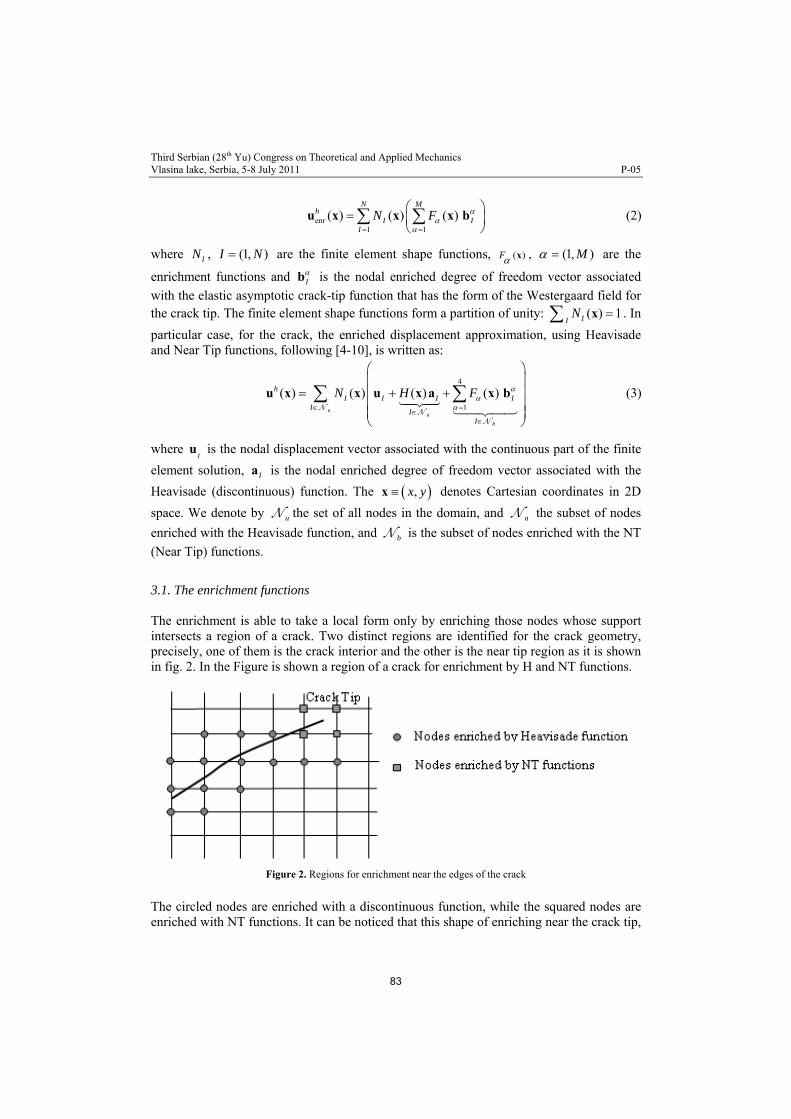
Third Serbian (28th Yu) Congress on Theoretical and Applied Mechanics Vlasina lake, Serbia, 5-8 July 2011 P-05
enr1 1
( ) ( ) ( )N M
hI I
I
N F
u x x x b
(2)
where IN , (1, )I N are the finite element shape functions, , ( )F x (1, )M are the
enrichment functions and Ib is the nodal enriched degree of freedom vector associated
with the elastic asymptotic crack-tip function that has the form of the Westergaard field for the crack tip. The finite element shape functions form a partition of unity: ( )II
N 1 x . In
particular case, for the crack, the enriched displacement approximation, using Heavisade and Near Tip functions, following [4-10], is written as:
4
1
( ) ( ) ( ) ( )u
a
b
hI I I I
II
I
N H F
u x x u x a x b
(3)
where I
u is the nodal displacement vector associated with the continuous part of the finite
element solution, Ia is the nodal enriched degree of freedom vector associated with the
Heavisade (discontinuous) function. The ,x yx denotes Cartesian coordinates in 2D
space. We denote by u the set of all nodes in the domain, and a the subset of nodes
enriched with the Heavisade function, and b is the subset of nodes enriched with the NT
(Near Tip) functions.
3.1. The enrichment functions The enrichment is able to take a local form only by enriching those nodes whose support intersects a region of a crack. Two distinct regions are identified for the crack geometry, precisely, one of them is the crack interior and the other is the near tip region as it is shown in fig. 2. In the Figure is shown a region of a crack for enrichment by H and NT functions.
Figure 2. Regions for enrichment near the edges of the crack
The circled nodes are enriched with a discontinuous function, while the squared nodes are enriched with NT functions. It can be noticed that this shape of enriching near the crack tip,
83

Third Serbian (28th Yu) Congress on Theoretical and Applied Mechanics Vlasina lake, Serbia, 5-8 July 2011 P-05
is used in [6-10]. In this paper we modified the modality of the nodes enriching near the crack tip (see next sections).
3.1.1 Generalized heavisade function The interior of the crack ( is the enrichment – domain) is modeled by the generalized
Heavisade enrichment function , where takes the value +1 above the crack and
–1 below the crack [6-10]:
c( )H X ( )H X
Figure 3. Illustration of the values of Heaviside function above and below of the crack
*1 if ( ) 0
( )*1 if ( ) 0
H
X X nX
X X n (4)
where is the sample (Gauss) point, (lies on the crack) is the closest point to , and
is unit outward normal to crack at (see fig. 3).
X *X*X
X
nIt can be seen that in the first published works [2], [3] above shape modeling of the discontinuity was not used. The formulation (4) begins to use due to practical numerical reasons.
3.1.2 The near-tip crack functions The crack tip enriched functions ensure that the crack terminates precisely at the location of the crack-tip. The linear elastic asymptotic crack-tip fields serve as suitable enrichment functions for providing the correct near-tip behavior, and in addition, their use also leads to better accuracy on relatively coarse finite element meshes in 2D [2-10]. The crack tip enrichment functions in isotropic elasticity have form of the Westergaard field for the crack tip:
1 2 3 4( ) , , , cos , sin , sin sin , cos sin2 2 2 2
F F F F F r r r r
x (5)
where and r denote polar coordinates in the local system at the crack tip. It can be noted that the second function of the set (5) is discontinuous over there crack faces [2], [3]. The discontinuity over the crack faces can be obtained using other functions like Heavisade
84

Third Serbian (28th Yu) Congress on Theoretical and Applied Mechanics Vlasina lake, Serbia, 5-8 July 2011 P-05
function (3), which have discontinuity. Let the element which contain the crack tip is denoted as CT element. In the papers [6-10] the discontinuity behind the tip in the CT element is accomplished by second function of the set (5). In this paper, the discontinuity in the CT element we have achieved with Heavisade function (4).
3.2. The level set representation of the crack In this paper a crack is presented using the set of the linear segments. The crack is described by means of the tip position and level set of a vector valued mapping. A signed distance function ( ) x is defined over computational domain using:
*( ) ( ) minc
sign
xx n X X X X* (6)
where is the unit normal to and is the closest point to , see fig. 3. The crack is
then represented as the zero level set of the function
n c*X X
( ) X , i.e.:
( ) 0 X (7)
The position related to the crack tip is defined through the following functions:
( ) ( )CT X X X t (8)
where is the unit tangent to at the crack tip t c c and is coordinate of . The value CTX c( ) 0 X corresponds to the crack tip. We defined LS functions ( ) X and ( ) X in the
whole computational domain. The crack and the crack tip are represented like:
(9) : ( , ) 0 ( , ) 0c t t X X X
In fig. 4, the definition of the ( ) x and ( ) x around the crack is shown. For the crack
representations linear interpolation has been used.
Figure 4. Definition of the level set functions ( ) X and ( ) X around the crack
The Heavisade step function (4) is modified using the LS function ( , )t X :
85

Third Serbian (28th Yu) Congress on Theoretical and Applied Mechanics Vlasina lake, Serbia, 5-8 July 2011 P-05
0
0
1 ( )( ( ))
1 ( )
ifH
if
XX
X (10)
The Near Tip functions ( , ), 1,4F r , that have form of the Westergaard field for the
crack tip [3], also should be defined using the LS functions [6-9], to obtain polar coordinates in the local system at the crack tip (see fig. 5):
2 2 1 ( )( ) ( ) ( ) ( ) tan .
( )r and
X
X X X XX
(11)
Apart from the other authors [6-10] we used NT functions only ahead the crack tip ( ( , ) 0t X ), while behind the crack tip ( ( , ) 0t X ), we ensured discontinuity across the
crack ( ( , ) 0t X ), using only the step function ( ( ))H X . Therefore, the Westergaard
field was used only for derivation of the asymptotic stress field ahead of the location near the tip i.e., ( , )t 0 X [6-9].
4. Element free Galerkin method Unlike the representational methods discussed mesh free methods rely on a field solver different from standard FEM. EFG method is a mesh free method in which the approximating function is a linear combination of a basis function and is fit to data by a weighted quadratic function. The Moving Least-Square (MLS) approximation constructed entirely in terms of a set of interior nodes and a description of the boundaries of the model. The value of the desired function i.e., displacements, at any point is obtained by solving a set of linear equations [11-15].
Figure 5. Free points domain in relation to integration point
86
Third Serbian (28th Yu) Congress on Theoretical and Applied Mechanics Vlasina lake, Serbia, 5-8 July 2011 P-05
the EFG method, due to the application of the MLS a
is [11-15]:
he
oef hich are the functions of spatial coor
two-d i
In pproximation, displacement
( , , ) ( )h hu x y z u x
1
( ) ( ) ( ) ( ) ( )m
h Tj j
j
u p a
x x x p x a x (12)
where ( )p x are the basis functions of the coordinates of free points, and ( )a x are tj
ficients, wj
c dinates x . In general case, the basis
functions for imensional problems (in th s paper, we have used linear base m =3):
( ) [1, , ]T x yp x (13)
oefficients in (12) for every point has obtained b
form:
(14)
e t
C y minimization of middling ( )a x x
2
1
( ) ( )[ ( ) ( ) ]n IT
I II
w u
x x p x a x
and hav he value:
1( ) ( ) ( )Ta x A x P W x u (15)
: where Iu is displacement of the free point I weight function of the free point I, and
ber of free points which influence to t
efined in the following way:
(16)
here:
, ( )Iw x
n he integration point, fig. 5. Matrix is the num
s d( )A x ha
( ) ( )TA x P W x P
w( )IJ J Jw w IJ x x (17)
and T
I IP p (18)
In the EFG method, the weight functions ( )w x are generally monotonously falling
functions of distanceI
Ix x
( )a x from
. These functions i nce to the displacement . This
is obvious when (16) is replaced in this paper, we used d
rm of weight function:
nflue
(12). In
( )hu x
the followe
fo22
max
2 max
max
( )1
0
max
kk II II
k III
I
ddcc
I
e ed d
9) d
I Ic
I
w de
d d
(1
87

Third Serbian (28th Yu) Congress on Theoretical and Applied Mechanics Vlasina lake, Serbia, 5-8 July 2011 P-05
here Ix to interpolated point x , and max I
d I Id x xw is distance from free point
defines the maximal area of weight function influe ce for each free point–influence radius.
Coefficient
n
c has differently defined in literature. In this paper, we have used definition
ccording to [14-15]: a max I
c d (20)
In this case, the recommendation for the value of is 0.4. We have adopted value for the coefficient 1Ik .
5 gral . Equialent domain integral method (EDI) for evaluation J-inte
6] r J-integral for two-dimensional crack s als. As shown in the fig. 6, J is the line
integral surrounding a two-dimensional crack tip and is defined as:
Rice [1 defined a path-independent contouproblem in linear and nonlinear elastic materi
1 1 ,10lim , , 1,2
Sj ij i jJ W u n d i j
S
where W is the strain nergy density give by:
e n
(21)
1 1W C , , , , 1, 2
2 2ij ij ijkl kl ij i j k l (22)
and jn is the outward normal vector to the contour integration, S is around the crack tip
(as s wn in fig. 6)ho , ij is stress tensor, ij is strain tensor, is constitutive tensor and
ponent of the displacement.
ijC kl
iu is com of vector
Figure 6. Conversion of the contour integral into an EDI
88

Third Serbian (28th Yu) Congress on Theoretical and Applied Mechanics Vlasina lake, Serbia, 5-8 July 2011 P-05
ntegral given (21) is rewritten, by int the ED en efine the w o
d (23)
where is contour (fig. 6),
The EDI approach has the advantage that the effect of variable body forces can be included easily. The standard J-contour i by Eq. roducing a weight function ,q x x into I. H ce, we d follo ing cont ur integral: 1 2
1(W ,1 )j ij i ju m q
0 S jm is a unit vector outward normal to the
orresponding contour (i.e. j jm n and j jm n c on 0 on S ), and is a
functio
q weight
n defined as 1q inside the contour and 0q for the doma de .
Taking the limit
in outsi 0S leads to [18, 19]:
,
4)
pplying the divergence theorem to Eq. (24), we obtain the
0
,0
,
lim ( )
lim ( ) lim
SSkj ij i k j
kj ij i k j
W u m qd
W u m qd
(2
0
,0 0
0 0( ) .
S S
S S
kj ij i k j
kj ij i k jW u m qd
lim lim ( )W u m qd
S
A following expression:
, , ,,
k ij i k kj j ij i k kjA A jJ u W q dA u W qdA (25)
wvanish
here is the area enclosed by . Note that the addend in the above equation must for linear-elastic materials [6, 17, 20], so we have: A G
, ,k ij i k kj jAJ u W q d A (26)
. Due to fact that there is no analytical solution for this xample, numerical results obtained with EFG and XFEM were compared with
corresponding ones obtained using standard FEM. In the standard FEM and EFG method, 2D mesh with eight nodes per element is used. In the XFEM, linear four nodes elements are used. Effective stress for 2D turbine model without insulation, for the crack length 30 mm using FEM and XFEM is shown in fig. 7.
This expression is analogous to the one proposed for a Surface Integral Based Method, to evaluate stress intensity factors.
7. Numerical example In this example the stress intensity factor of the crack located in the steam turbine housing 4 Thermal plant Kolubara is calculatede
89
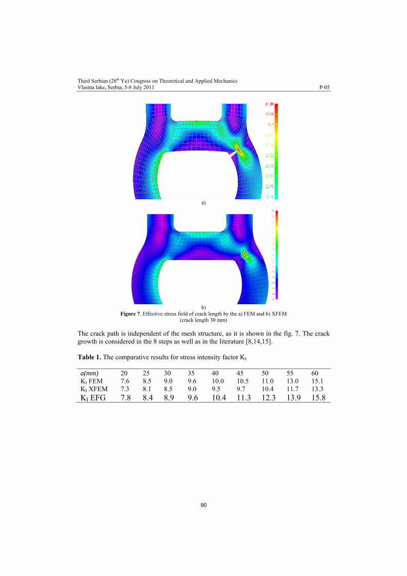
Third Serbian (28th Yu) Congress on Theoretical and Applied Mechanics Vlasina lake, Serbia, 5-8 July 2011 P-05
b) Figure 7. Effective stress field of crack length by the a) FEM and b) XFEM
(crack length 30 mm)
The crack path is independent of the mesh structure, as it is shown in the fig. 7. The crack growth is considered in the 8 steps as well as in the literature [8,14,15]. Table 1. The comparative results for stress intensity factor KI
a(mm) 20 25 30 35 40 45 50 55 60
a)
KI FEM 7.6 8.5 9.0 9.6 10.0 10.5 11.0 13.0 15.1 KI XFEM 7.3 8.1 8.5 9.0 9.5 9.7 10.4 11.7 13.3 KI EFG 7.8 8.4 8.9 9.6 10.4 11.3 12.3 13.9 15.8
90

Third Serbian (28th Yu) Congress on Theoretical and Applied Mechanics Vlasina lake, Serbia, 5-8 July 2011 P-05
FEM
XFEM
EFG
20.00 25.00 30.00 35.00 40.00 45.00 50.00 55.00 60.00 65.00
0
2
4
6
Crack length [mm] Figure 8. Relationship between Stress Intensity Factor KI and crack length
The results shown in the Table 1 were obtained using standard FEM, EFG and XFEM. The J-EDI approach for defining stress intensity factor was used in those methodologies. We have displayed only the opening mode stress intensity factor, KI, because it is dominating in this example. In the fig. 8, the relationship between stress intensity factor KI and crack length is shown. Increasing of the crack length from 20 mm to 60 mm causes increasing of the stress intensity factor, as it is illu
12
14
16
18
]1/2
8
10
strated in the fig. 8. The some difference in numerical sults colud be adressed to different order of element interpolation which is used in the FEM and EFG.
8. Conclusion
n by relatively high values
pproaches, some numerical method
(LSM). In the XFEM the Finite-element approximation is enriched by appropriate functions
natural since the enrichment can be described and even constructed in terms of level set
d programme is based on the standard FEM, EFG and XFEM. The advantage of XFEM and EFG related
Str
ess
Inte
sity
Fac
tor
[MP
am
reX
Crack propagation is a process of evolutionary geometry driveand gradients in crack front fields. The integration of all three fundamental aspect of the problem – computing local field quantities, ascertaining resulting material damage, and evolving the crack- can be had with a reach variety of aas well as: XFEM, EFG, LSM, J-EDI. For the numerical simulation we apply a combination of the eXtended Finite-element method (XFEM) and the Level Set Method
through the concept of partition of unity. The geometry of material interfaces and cracks is described by the LSM. The combination of both, XFEM and LSM, turns out to be very
functions. The programme was write in FORTRAN and integrated in PAK FM&F [10] for considering different methodologies and its influence on the results. Develope
to the standard FEM is feasibility to use fixed finite element mesh, whereby the crack growth is independent of the mesh.
91

Third Serbian (28th Yu) Congress on Theoretical and Applied Mechanics Vlasina lake, Serbia, 5-8 July 2011 P-05
and I. Babuska, The partition of unity finite element method: Basic theory and applications.
Numerical Methods in Engineering. 45(5):601-620,1999.
:131-150,1999.
merical Methods in Engineering 48(12),1741-1760, 2000.
lids and Structures 40,7513-7537, 2003.
2005.
20
ć, D., Improvement of algorithm for numerical
owth by Element Free Galerkin Methods,
namic Fracture Problems Using the Element-Free Galerkin Method,
e, First South-East European Conference on Computational echanics, SEECCM-06, Kragujevac, 2006.
[15] Jovičić G., Živković M., Vukadinović V., Numerical Methods for Determination of krack Growth of the Real Structure, 1ST International Congress of Serbian Society of Mechanics- IConSSM –Kopaonik, 2007.
[16] Rice J.R., A Path Independent Integral and Approximate Analysis of Strain Concentration by Notches and Cracks, Journal of Applied Mechanics, 35, 379-386, 1968.
5. References
[1] J. M. Melenk Computer Methods in Applied Mechanics and Engineering 39, 289-314, 1996.
[2] T. Belytschko and T. Black, Elastic crack growth in finite elements with minimal remeshing. International Journal for
[3] N. Moes, J. Dolbow, and T. Belytschko, A finite element method for crack growth without remeshing. International Journal for Numerical Methods in Engineering. 46(1)
[4] C. Daux, N. Moes, J.Dolbow, N. Sukumur, T. Belytschko, Arbitrary cracks and holes with the extended finite element method, International Journal for Nu
[5] Sukumur N. and J.H. Prevost, Modeling quasi-static crack growth with the extended finite element method Part I: Computer implementation, International Journal of So
[6] Jovičić G., An Extended Finite Element Method for Fracture Mechanics and Fatigue Analysis, Ph. D. Thesis, Faculty of Mechanical Engineering, University Kragujevac,
[7] Jovičić G., Živković M., Jovičić N., Numerical Simulation of Crack Modeling using Extended Finite Element Method, Journal of Mechanical Engineering, Vol.55, No.9 pp. 549-554, UDC 620.178, ISSN 0039-2480, 2009.
[8] Jovičić G., Grabulov V., Maksimović S., Živković M., Jovičić N., Bosković G., Maksimović K., Residual Life Estimation of Power Plant Component the High Pressure Turbine Housing Case, Thermal Science, Vol. 13, No. 4, pp. 99-106, 09
[9] Jovičić, G., Živković, M., Sedmak, A., Jovičić, N., Milovanovicrack modeling, Archieves of Civil and Mechanical Engineering, Vol. 10, No. 3, pp. 19-35, ISSN 1644-9665, 2010.
[10] Živković M., Jovičić G., Kojić M., Slavković R., Grujović N., Vulović S., PAK FM&F softvare, TR-22/2010, University of Kragujevac, Faculty of Mechanical Engineering,
[11] Belytschko T., Gu L., Lu Y.Y., Fracture and Crack GrNorthwestern university, Evanston, 1993.
[12] Organ J.D., Numerical Solutions to DyPhD thesis, Northwestern university, Evanston, 1996.
[13] Belytschko T., Krongaus Y., Organ D., Fleming M., Krysl P., Meshless methods: An Overview and Recent Developments, Northwestern University, Evanston, 1996.
[14] Živković M., Jovičić G., Vukadinović V., Đordjević N., Kojić M. , Comparison of EFG, X-FEM and FEM in Fracture Mechanics Analysis of Real StructurM
92
Third Serbian (28th Yu) Congress on Theoretical and Applied Mechanics Vlasina lake, Serbia, 5-8 July 2011 P-05
[17] Lin C-Y., Determination of the Fracture Parameters in a Stiffened Composite Panel, Ph.D. Thesis, North Carolina State University, 2000.
[18] Kim J.-H., Paulino G.H., Mixed-mode J-integral formulation and implementation using graded elements for fracture analysis of no homogeneous orthotropic materials, Mechanics of Materials 35 pp. 107-128; 2002.
[19] Enderlein M. Kuna M., Comparison of finite element techniques for 2D and 3D crack analysis under impact loading, International Journal for Solid and Structures, 40, 2003.
[20] Jovičić G., Živković M., Kojić M., Vulović S., Numerical programs for life assessment of the steam turbine housing of the thermal power plant, From Fracture Mechanics to Structural Integrity Assessment, Monography, Editors: S Sedmak, Z. Radaković, 2004.
[21] Rye A. M., Fatigue Crack Initiation and Growth in Ship Structures, PhD Thesis, Department of Naval Architecture and Offshore Engineering Technical University of Denmark, 1998.
[22] Iida S. and A. S. Kobayashi, “Crack-Propagation Rate in 7075-T6 Plates under Cyclic Tensile and Transverse Shear Loadings”, Journal of Basic Engineering, 764-769, 1969.
[23] Tanaka K., “Fatigue Crack Propagation from a Crack Inclined to the Cyclic Tensile Axis”, Engineering Fracture Mechanics, 6, 493-507, 1974.
93

Third Serbian (28th Yu) Congress on Theoretical and Applied Mechanics Vlasina lake, Serbia, 5-8 July 2011 P-06
REDUCED ORDER MODELS FOR ANALYSIS AND CONTROL OF NONLINEAR SYSTEMS WITH PERIODIC COEFFICIENTS
S. C. Sinha1 and A. Gabale2
1 Department of Mechanical Engineering Auburn University, Auburn, AL, USA e-mail: [email protected] 2 Corporate Research and Development, Cummins Inc., Columbus, IN, USA e-mail: [email protected]
ABSTRACT. This work presents some methodologies for order reduction of parametrically excited nonlinear systems subjected to external inputs. This important class of problems arises in the analysis and control of structures with rotating components and periodic in-plane loads or systems described by nonlinear differential equations representing dynamics about a periodic motion. The techniques presented are based on construction of a time-varying invariant manifold. Two types of inputs are considered; namely, an external periodic excitations and a nonlinear, stabilizing state feedback control.
In the first case we are interested in approximating an dimensional time-periodic nonlinear system of the form
n
( ) ( , ) ( )rt t t x A x f x G (1)
by a system of differential equations of a smaller dimension
. In the above equation m n is a small positive number and is a given
periodic input. Order reduction for all three cases (viz., fundamental, sub and super harmonic) are considered. The second problem deals with Next we consider an order reduction of a parametrically excited nonlinear closed-loop system of the form
( )tG
0 1, ,r rt t t t u x Α x f x g g xu
(2)
where is a scalar state feedback. In both cases we apply Lyapunov-Floquét (LF) transformation and separate the dominant and the non-dominant (slave) states. Then the dominant dynamics represented by the reduced order model, can be decoupled from the non-dominant dynamics by constructing an invariant manifold relating the non-dominant states as nonlinear periodic functions of the dominant states [1]. The control problem (given by equation (2)) involves design of a linear as well as a nonlinear controller where the linear controller is designed using a symbolic approach that can place the Floquét multipliers in the desired locations [2]. Examples are included to demonstrate the effectiveness of the method.
Keywords: Floquét multipliers, Time-periodic systems, Lyapunov- Floquét transformation, Order reduction, Invariant manifold
References [1] Amit P. Gabale* and S. C. Sinha, Construction of Reduced Order Controllers for
Nonlinear Systems with Periodic Coefficients, To appear in Journal of Vibration and Control, 2010.
[2] Sinha, S. C., Gourdon, E., Zhang, Y., 2005, Control of time-periodic systems via symbolic computation with application to chaos control, Communications in Nonlinear Science and Numerical Simulations, 10, pp. 835-854.
94