A wind profiler trajectory tool for air quality transport applications

A wind profiler trajectory tool for air quality transport applications

Allen B. White,1,2 Christoph J. Senff,1,2 Ann N. Keane,3 Lisa S. Darby,3

Irina V. Djalalova,1,2 Dominique C. Ruffieux,1,4 David E. White,1,2

Brent J. Williams,5 and Allen H. Goldstein5

Received 3 May 2006; revised 13 September 2006; accepted 27 September 2006; published 12 December 2006.

[1] Horizontal transport is a key factor in air pollution meteorology. In several recentair quality field campaigns, networks of wind profiling Doppler radars have been deployedto help characterize this important phenomenon. This paper describes a Lagrangianparticle trajectory tool developed to take advantage of the hourly wind observationsprovided by these special profiler networks. The tool uses only the observed wind profilesto calculate trajectory positions and does not involve any model physics orparameterizations. An interpolation scheme is used to determine the wind speed anddirection at any given location and altitude along the trajectory. Only the horizontal windsmeasured by the profilers are included because the type of profiling radars used in thisstudy are unable to resolve synoptic-scale vertical motions. The trajectory tool is appliedto a case study from the International Consortium for Research on Transportand Transformation air quality experiment conducted during the summer of 2004(ICARTT-04). During this international field study, air chemistry observations werecollected at Chebogue Point, a coastal station in southwestern Nova Scotia, and factoranalysis was used to identify time periods when air pollution from the United Statesarrived at the site. The profiler trajectories are compared to trajectories produced fromnumerical model initialization fields. The profiler-based trajectories more accuratelyreflect changes in the synoptic weather pattern that occurred between operational upper airsoundings, thereby providing a more accurate depiction of the horizontal transportresponsible for air pollution arriving in Nova Scotia.

Citation: White, A. B., C. J. Senff, A. N. Keane, L. S. Darby, I. V. Djalalova, D. C. Ruffieux, D. E. White, B. J. Williams, and

A. H. Goldstein (2006), A wind profiler trajectory tool for air quality transport applications, J. Geophys. Res., 111, D23S23,

doi:10.1029/2006JD007475.

1. Introduction

[2] Lagrangian-based particle trajectory models are usefulfor studying the transport of atmospheric constituents suchas aerosols, ozone, and water vapor. Several model-basedtrajectory tools already exist. The HYbrid Single-ParticleLagrangian Integrated Trajectory (HYSPLIT) model devel-oped by the NOAA Air Resources Laboratory (http://www.arl.noaa.gov/ready/hysplit4.html) and the FLEXPARTmodel developed by the Norwegian Institute of AirResearch (http://zardoz.nilu.no/�andreas/flextra+flexpart.html) are two commonly used approaches.[3] The NOAA Earth System Research Laboratory

(NOAA/ESRL) has developed an observationally based

trajectory tool that uses data from wind profiler networksto calculate forward or backward particle trajectories. Thetool is purely observationally based, i.e., there are no modelphysics or parameterizations involved. The trajectory algo-rithm applies an inverse distance squared weighting func-tion to the observations from profiler networks in order todetermine the hourly position of the trajectories.[4] The profiler trajectory tool was first developed for the

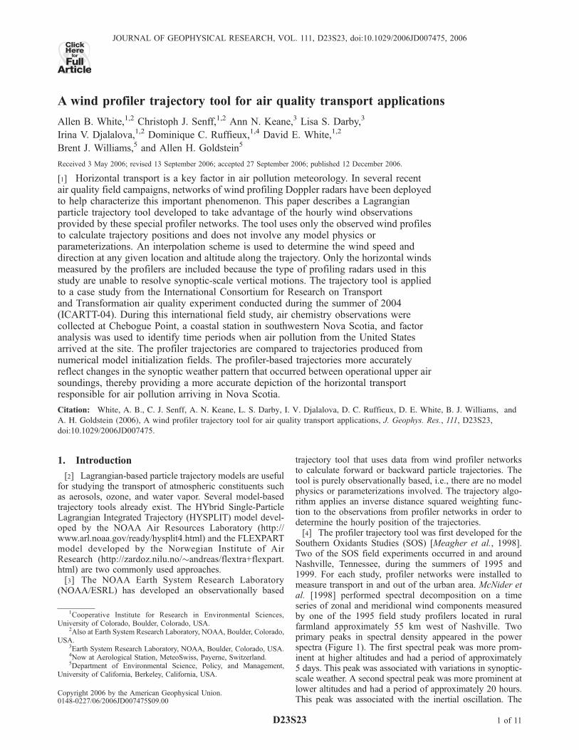
Southern Oxidants Studies (SOS) [Meagher et al., 1998].Two of the SOS field experiments occurred in and aroundNashville, Tennessee, during the summers of 1995 and1999. For each study, profiler networks were installed tomeasure transport in and out of the urban area. McNider etal. [1998] performed spectral decomposition on a timeseries of zonal and meridional wind components measuredby one of the 1995 field study profilers located in ruralfarmland approximately 55 km west of Nashville. Twoprimary peaks in spectral density appeared in the powerspectra (Figure 1). The first spectral peak was more prom-inent at higher altitudes and had a period of approximately5 days. This peak was associated with variations in synoptic-scale weather. A second spectral peak was more prominent atlower altitudes and had a period of approximately 20 hours.This peak was associated with the inertial oscillation. The

JOURNAL OF GEOPHYSICAL RESEARCH, VOL. 111, D23S23, doi:10.1029/2006JD007475, 2006ClickHere

for

FullArticle

1Cooperative Institute for Research in Environmental Sciences,University of Colorado, Boulder, Colorado, USA.

2Also at Earth System Research Laboratory, NOAA, Boulder, Colorado,USA.

3Earth System Research Laboratory, NOAA, Boulder, Colorado, USA.4Now at Aerological Station, MeteoSwiss, Payerne, Switzerland.5Department of Environmental Science, Policy, and Management,

University of California, Berkeley, California, USA.

Copyright 2006 by the American Geophysical Union.0148-0227/06/2006JD007475$09.00

D23S23 1 of 11

http://dx.doi.org/10.1029/2006JD007475

inertial period is given by 2p/f, where f is the Coriolisparameter. For the profiler site used in this analysis, f =8.624 � 10�5 s�1. The theoretical inertial period is then 20.2hours, which agrees well with the period of the observedspectral peak in the zonal and meridional wind componentpower spectra produced from the wind profiler data.[5] Under weak synoptic forcing, a nocturnal low-level

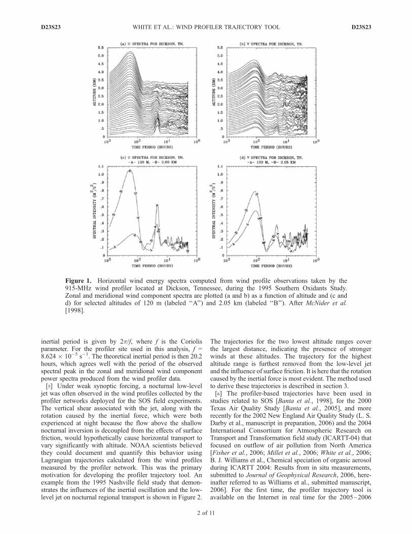
jet was often observed in the wind profiles collected by theprofiler networks deployed for the SOS field experiments.The vertical shear associated with the jet, along with therotation caused by the inertial force, which were bothexperienced at night because the flow above the shallownocturnal inversion is decoupled from the effects of surfacefriction, would hypothetically cause horizontal transport tovary significantly with altitude. NOAA scientists believedthey could document and quantify this behavior usingLagrangian trajectories calculated from the wind profilesmeasured by the profiler network. This was the primarymotivation for developing the profiler trajectory tool. Anexample from the 1995 Nashville field study that demon-strates the influences of the inertial oscillation and the low-level jet on nocturnal regional transport is shown in Figure 2.

The trajectories for the two lowest altitude ranges coverthe largest distance, indicating the presence of strongerwinds at these altitudes. The trajectory for the highestaltitude range is furthest removed from the low-level jetand the influence of surface friction. It is here that the rotationcaused by the inertial force is most evident. The method usedto derive these trajectories is described in section 3.[6] The profiler-based trajectories have been used in

studies related to SOS [Banta et al., 1998], for the 2000Texas Air Quality Study [Banta et al., 2005], and morerecently for the 2002 New England Air Quality Study (L. S.Darby et al., manuscript in preparation, 2006) and the 2004International Consortium for Atmospheric Research onTransport and Transformation field study (ICARTT-04) thatfocused on outflow of air pollution from North America[Fisher et al., 2006; Millet et al., 2006; White et al., 2006;B. J. Williams et al., Chemical speciation of organic aerosolduring ICARTT 2004: Results from in situ measurements,submitted to Journal of Geophysical Research, 2006, here-inafter referred to as Williams et al., submitted manuscript,2006]. For the first time, the profiler trajectory tool isavailable on the Internet in real time for the 2005–2006

Figure 1. Horizontal wind energy spectra computed from wind profile observations taken by the915-MHz wind profiler located at Dickson, Tennessee, during the 1995 Southern Oxidants Study.Zonal and meridional wind component spectra are plotted (a and b) as a function of altitude and (c andd) for selected altitudes of 120 m (labeled ‘‘A’’) and 2.05 km (labeled ‘‘B’’). After McNider et al.[1998].

D23S23 WHITE ET AL.: WIND PROFILER TRAJECTORY TOOL

2 of 11

D23S23

Texas air quality study (TEXAQS-II). In section 4 we applythe profiler-based trajectory method to a case study fromICARTT-04.

2. Wind Profilers

[7] Wind profilers are Doppler radars that operate mostoften in the UHF or VHF frequency bands. Four primarytypes of wind profilers were in operation in the UnitedStates at the time of this publication. The NOAA ProfilerNetwork (NPN) profilers are fixed radars that operate at afrequency of 404 MHz [Chadwick, 1988], although afrequency conversion to 449 MHz has been mandated bythe Federal Communications Commission. A smaller, trans-portable, wind profiler used by NOAA research and otheragencies is the 915-MHz boundary layer wind profiler[Carter et al., 1995]. The NPN profilers provide the deepestcoverage of the atmosphere, but lack coverage in theplanetary boundary layer (PBL). The 915-MHz profilersprovide the best coverage of winds in the PBL, but they lackheight coverage much above the PBL. A third type of windprofiler that operates at 449 MHz (the so-called1=4-scale 449-MHz profiler) combines the best sampling attributes of theother two systems. The U.S. Air Force has recently installedseveral of these radars along the southern U.S. border. The50-MHz wind profiler is the oldest type of radar windprofiler produced in the United States [Ecklund et al.,1979]. It is useful for deep atmospheric probing, butprovides very little information in the boundary layer[Frisch et al., 1986].

[8] Wind profilers transmit pulses of electromagneticradiation vertically and in at least two slightly off-vertical(�75� elevation) directions in order to resolve the three-dimensional vector wind. A small amount of the energytransmitted in each direction is reflected or backscattered tothe radar antenna. The backscatter returns are Dopplershifted by the motion of the scattering media. Profilersreceive backscatter returns from atmospheric features (tur-bulence, clouds, precipitation) and nonatmospheric features(insects, birds, trees, airplanes, radio-frequency interfer-ence). The challenge in signal processing is to avoid thereturns from nonatmospheric scattering targets and focus onthe atmospheric returns. To do this, profilers samplethousands of consecutive transmitted pulses to boost thesignal-to-noise ratio of the atmospheric returns, a processknown as ‘‘coherent integration.’’[9] The return signals are sampled at discrete intervals

called range gates. The size of the range gates is determinedby the length of the transmitted pulse, which is usually onthe order of hundreds to thousands of nanoseconds (ns). Forexample, a 700-ns pulse translates into a true range resolu-tion (i.e., one without oversampling) of 105 m. Once therange-gated Doppler shifts from a set of beams have beendetermined, a wind profile is calculated. This processusually occurs over an observing period of 30 to 90 s.The wind profiles measured within a specified averagingperiod (15 min to 60 min) are averaged together using aconsensus routine. The consensus routine filters outliersusing threshold and acceptance windows. The consensuswind profiles are archived on site and transmitted back to adata hub in Boulder, Colorado, via phone lines or, in remoteareas, via satellite communications. Postprocessing dataquality control is applied using the continuity methoddeveloped by Weber et al. [1993]. The accuracy of hori-zontal winds measured by the profiler is better than 1 m s�1

on the basis of comparison with balloon soundings [Martneret al., 1993]. The accuracy of profiler vertical-velocitymeasurements is less certain [e.g., Worthington, 2002].

3. Wind Profiler Trajectory Tool

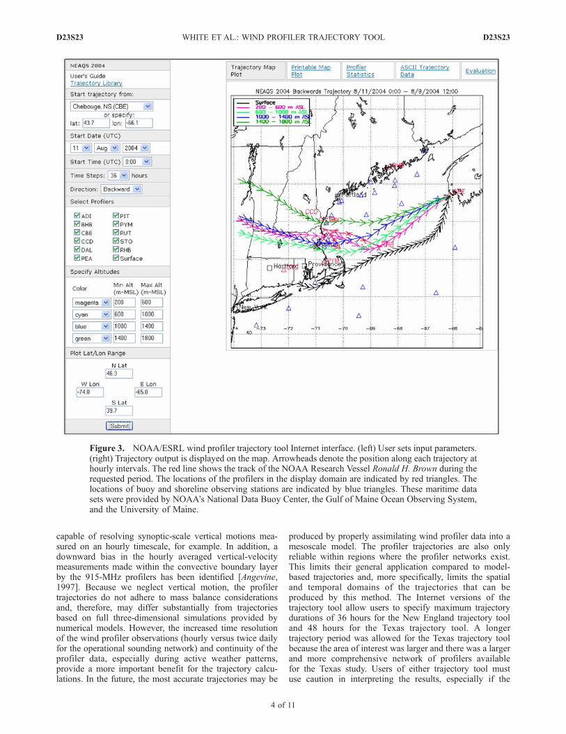
[10] The wind profiler data arriving from field sites areconverted to a common format and placed in a database foruse by the trajectory tool. The tool can be used in post-experiment analysis activities, and beginning with theTEXAQS-II study in 2005 (http://esrl.noaa.gov/csd/2006/),in near real time to support mission planning activitiesand NWS forecast operations (see http://www.etl.noaa.gov/programs/2006/texaqs/traj/). The user has the optionof calculating forward or backward trajectories and speci-fying the start/end point location and the period over whichto calculate the trajectories. Other options include specify-ing multiple altitude ranges and the number of profilers touse or exclude in the calculations. For locations over water,the user may request surface trajectories that are producedfrom available buoy and shoreline surface wind observa-tions and upper air trajectories that include wind profileobservations from the NOAA Research Vessel Ronald H.Brown, when available (see Figure 3 or http://www.etl.noaa.gov/programs/2004/neaqs/traj/).[11] The profiler trajectory tool uses only the horizontal

winds measured by the profilers. Wind profilers are not

Figure 2. Forward trajectories for the dates, times, andaltitudes shown at the bottom left. The trajectories arecalculated from wind profiler observations collected duringthe 1995 Southern Oxidants Study Nashville/MiddleTennessee intensive. The locations of the wind profilersare indicated by the stars. These overnight trajectoriesdemonstrate the combined effects of a nocturnal low-leveljet and the inertial oscillation on regional transport.


3 of 11

D23S23

capable of resolving synoptic-scale vertical motions mea-sured on an hourly timescale, for example. In addition, adownward bias in the hourly averaged vertical-velocitymeasurements made within the convective boundary layerby the 915-MHz profilers has been identified [Angevine,1997]. Because we neglect vertical motion, the profilertrajectories do not adhere to mass balance considerationsand, therefore, may differ substantially from trajectoriesbased on full three-dimensional simulations provided bynumerical models. However, the increased time resolutionof the wind profiler observations (hourly versus twice dailyfor the operational sounding network) and continuity of theprofiler data, especially during active weather patterns,provide a more important benefit for the trajectory calcu-lations. In the future, the most accurate trajectories may be

produced by properly assimilating wind profiler data into amesoscale model. The profiler trajectories are also onlyreliable within regions where the profiler networks exist.This limits their general application compared to model-based trajectories and, more specifically, limits the spatialand temporal domains of the trajectories that can beproduced by this method. The Internet versions of thetrajectory tool allow users to specify maximum trajectorydurations of 36 hours for the New England trajectory tooland 48 hours for the Texas trajectory tool. A longertrajectory period was allowed for the Texas trajectory toolbecause the area of interest was larger and there was a largerand more comprehensive network of profilers availablefor the Texas study. Users of either trajectory tool mustuse caution in interpreting the results, especially if the

Figure 3. NOAA/ESRL wind profiler trajectory tool Internet interface. (left) User sets input parameters.(right) Trajectory output is displayed on the map. Arrowheads denote the position along each trajectory athourly intervals. The red line shows the track of the NOAA Research Vessel Ronald H. Brown during therequested period. The locations of the profilers in the display domain are indicated by red triangles. Thelocations of buoy and shoreline observing stations are indicated by blue triangles. These maritime datasets were provided by NOAA’s National Data Buoy Center, the Gulf of Maine Ocean Observing System,and the University of Maine.


4 of 11

D23S23

trajectories pass outside the domain of the profiler network,where they become increasingly unreliable as the distancebetween the trajectory and the closest profiler observing siteincreases.[12] For each hour in the requested trajectory period, the

profiler trajectory algorithm uses all user-selected profilersin the network. The user has the option of deselecting one ormore of the profilers, for example, if it is known that aprofiler is malfunctioning, or to test the impact of aparticular profiler or a set of profilers on the trajectoryalgorithm output. The algorithm computes the distance fromthe trajectory start point to all requested profiler locations,calculates the average wind speed and direction using aninverse distance squared weighting function, and calculatesthe trajectory for the first hour. If the trajectory starts or endsabove a profiler location, or if the trajectory passes directlyover a profiler site, a minimum distance of 0.01 km isassigned in order to avoid dividing by zero. Then thisprocess is repeated for the remaining hours of the trajectoryperiod using the trajectory end point of the previous hour asthe reference point for the distance calculation. The weight-ing function technique is similar to creating a new set ofgridded profiler winds for each hour in the trajectory period.Creating a full grid is not necessary because we are onlyinterested in the one grid point that lies along the trajectory.

[13] If data from one of the requested profilers are notavailable at any given hour during the trajectory period,the weighted average will be computed from the remain-ing profilers. If the same profiler provides useable data ata later point in time during the trajectory period, it is againincluded in the average. If all selected profilers have adata outage at the same time, then the trajectory calcula-tion is stopped at the hourly time step preceding theoutage. No interpolation across data gaps is performed.Therefore a 1-hour data gap in all selected profilerstruncates the trajectory.[14] Profiler data measured at altitudes above mean sea

level (msl) that fall into each of the user-specified altitudebins are averaged together. A future version of the profilertrajectory tool will allow users to choose the vertical frameof reference for the profiler data; either above msl or aboveground level (agl). The agl frame of reference would bemore appropriate to use, for example, when calculating low-level trajectories over complex terrain.[15] Once the trajectory output has been plotted, the user

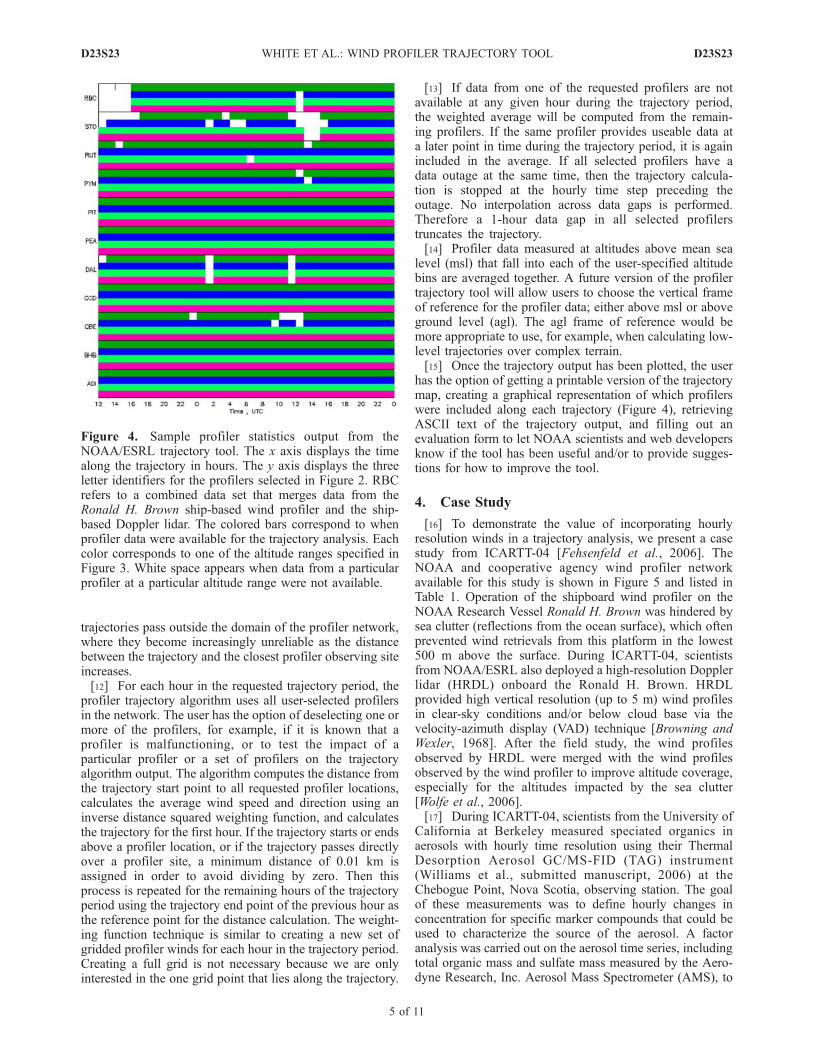
has the option of getting a printable version of the trajectorymap, creating a graphical representation of which profilerswere included along each trajectory (Figure 4), retrievingASCII text of the trajectory output, and filling out anevaluation form to let NOAA scientists and web developersknow if the tool has been useful and/or to provide sugges-tions for how to improve the tool.

4. Case Study

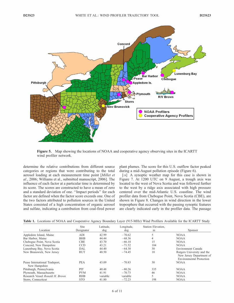
[16] To demonstrate the value of incorporating hourlyresolution winds in a trajectory analysis, we present a casestudy from ICARTT-04 [Fehsenfeld et al., 2006]. TheNOAA and cooperative agency wind profiler networkavailable for this study is shown in Figure 5 and listed inTable 1. Operation of the shipboard wind profiler on theNOAA Research Vessel Ronald H. Brown was hindered bysea clutter (reflections from the ocean surface), which oftenprevented wind retrievals from this platform in the lowest500 m above the surface. During ICARTT-04, scientistsfrom NOAA/ESRL also deployed a high-resolution Dopplerlidar (HRDL) onboard the Ronald H. Brown. HRDLprovided high vertical resolution (up to 5 m) wind profilesin clear-sky conditions and/or below cloud base via thevelocity-azimuth display (VAD) technique [Browning andWexler, 1968]. After the field study, the wind profilesobserved by HRDL were merged with the wind profilesobserved by the wind profiler to improve altitude coverage,especially for the altitudes impacted by the sea clutter[Wolfe et al., 2006].[17] During ICARTT-04, scientists from the University of

California at Berkeley measured speciated organics inaerosols with hourly time resolution using their ThermalDesorption Aerosol GC/MS-FID (TAG) instrument(Williams et al., submitted manuscript, 2006) at theChebogue Point, Nova Scotia, observing station. The goalof these measurements was to define hourly changes inconcentration for specific marker compounds that could beused to characterize the source of the aerosol. A factoranalysis was carried out on the aerosol time series, includingtotal organic mass and sulfate mass measured by the Aero-dyne Research, Inc. Aerosol Mass Spectrometer (AMS), to

Figure 4. Sample profiler statistics output from theNOAA/ESRL trajectory tool. The x axis displays the timealong the trajectory in hours. The y axis displays the threeletter identifiers for the profilers selected in Figure 2. RBCrefers to a combined data set that merges data from theRonald H. Brown ship-based wind profiler and the ship-based Doppler lidar. The colored bars correspond to whenprofiler data were available for the trajectory analysis. Eachcolor corresponds to one of the altitude ranges specified inFigure 3. White space appears when data from a particularprofiler at a particular altitude range were not available.


5 of 11

D23S23

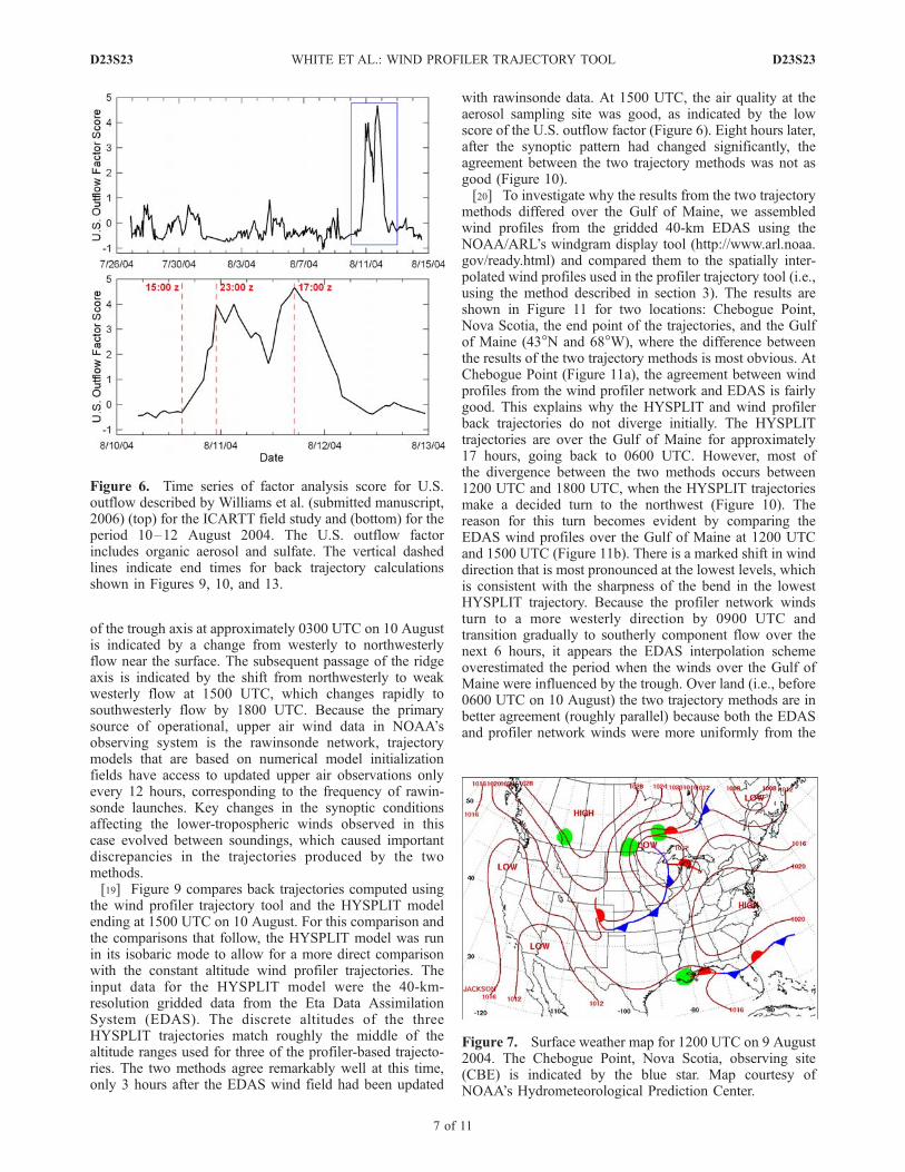
determine the relative contributions from different sourcecategories or regions that were contributing to the totalaerosol loading at each measurement time point [Millet etal., 2006; Williams et al., submitted manuscript, 2006]. Theinfluence of each factor at a particular time is determined byits score. The scores are constructed to have a mean of zeroand a standard deviation of one. ‘‘Impact periods’’ for eachfactor are defined when the factor score exceeds one. One ofthe two factors attributed to pollution sources in the UnitedStates consisted of a high concentration of organic aerosoland sulfate, indicating a contribution from coal-fired power

plant plumes. The score for this U.S. outflow factor peakedduring a mid-August pollution episode (Figure 6).[18] A synoptic weather map for this case is shown in

Figure 7. At 1200 UTC on 9 August, a trough axis waslocated to the west of Nova Scotia and was followed furtherto the west by a ridge axis associated with high pressurecentered over the mid-Atlantic U.S. coastline. The windprofiler data from Chebogue Point, Nova Scotia (CBE), areshown in Figure 8. Changes in wind direction in the lowertroposphere that occurred with the passing synoptic featuresare clearly indicated early in the profiler data. The passage

Figure 5. Map showing the locations of NOAA and cooperative agency observing sites in the ICARTTwind profiler network.

Table 1. Locations of NOAA and Cooperative Agency Boundary Layer (915-MHz) Wind Profilers Available for the ICARTT Study

LocationSite

DesignatorLatitude,

degLongitude,

degStation Elevation,

m Sponsor

Appledore Island, Maine ADI 42.99 �70.62 5 NOAABar Harbor, Maine BHB 44.44 �68.36 4 NOAAChebogue Point, Nova Scotia CBE 43.70 �66.10 15 NOAAConcord, New Hampshire CCD 43.21 �71.52 104 NOAALunenburg Bay, Nova Scotia DAL 44.40 �64.30 30 Environment CanadaNew Brunswick, New Jersey RUT 40.50 �74.45 10 Rutgers University and the

New Jersey Department ofEnvironmental Protection

Pease International Tradeport,New Hampshire

PEA 43.09 �70.83 30 NOAA

Pittsburgh, Pennsylvania PIT 40.48 �80.26 335 NOAAPlymouth, Massachusetts PYM 41.91 �70.73 46 NOAAResearch Vessel Ronald H. Brown RHB variable variable 5 NOAAStorrs, Connecticut STO 41.80 �72.23 198 NOAA


6 of 11

D23S23

of the trough axis at approximately 0300 UTC on 10 Augustis indicated by a change from westerly to northwesterlyflow near the surface. The subsequent passage of the ridgeaxis is indicated by the shift from northwesterly to weakwesterly flow at 1500 UTC, which changes rapidly tosouthwesterly flow by 1800 UTC. Because the primarysource of operational, upper air wind data in NOAA’sobserving system is the rawinsonde network, trajectorymodels that are based on numerical model initializationfields have access to updated upper air observations onlyevery 12 hours, corresponding to the frequency of rawin-sonde launches. Key changes in the synoptic conditionsaffecting the lower-tropospheric winds observed in thiscase evolved between soundings, which caused importantdiscrepancies in the trajectories produced by the twomethods.[19] Figure 9 compares back trajectories computed using

the wind profiler trajectory tool and the HYSPLIT modelending at 1500 UTC on 10 August. For this comparison andthe comparisons that follow, the HYSPLIT model was runin its isobaric mode to allow for a more direct comparisonwith the constant altitude wind profiler trajectories. Theinput data for the HYSPLIT model were the 40-km-resolution gridded data from the Eta Data AssimilationSystem (EDAS). The discrete altitudes of the threeHYSPLIT trajectories match roughly the middle of thealtitude ranges used for three of the profiler-based trajecto-ries. The two methods agree remarkably well at this time,only 3 hours after the EDAS wind field had been updated

with rawinsonde data. At 1500 UTC, the air quality at theaerosol sampling site was good, as indicated by the lowscore of the U.S. outflow factor (Figure 6). Eight hours later,after the synoptic pattern had changed significantly, theagreement between the two trajectory methods was not asgood (Figure 10).[20] To investigate why the results from the two trajectory

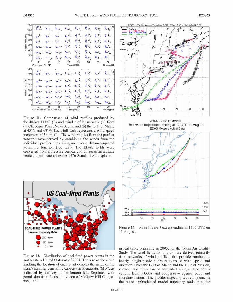
methods differed over the Gulf of Maine, we assembledwind profiles from the gridded 40-km EDAS using theNOAA/ARL’s windgram display tool (http://www.arl.noaa.gov/ready.html) and compared them to the spatially inter-polated wind profiles used in the profiler trajectory tool (i.e.,using the method described in section 3). The results areshown in Figure 11 for two locations: Chebogue Point,Nova Scotia, the end point of the trajectories, and the Gulfof Maine (43�N and 68�W), where the difference betweenthe results of the two trajectory methods is most obvious. AtChebogue Point (Figure 11a), the agreement between windprofiles from the wind profiler network and EDAS is fairlygood. This explains why the HYSPLIT and wind profilerback trajectories do not diverge initially. The HYSPLITtrajectories are over the Gulf of Maine for approximately17 hours, going back to 0600 UTC. However, most ofthe divergence between the two methods occurs between1200 UTC and 1800 UTC, when the HYSPLIT trajectoriesmake a decided turn to the northwest (Figure 10). Thereason for this turn becomes evident by comparing theEDAS wind profiles over the Gulf of Maine at 1200 UTCand 1500 UTC (Figure 11b). There is a marked shift in winddirection that is most pronounced at the lowest levels, whichis consistent with the sharpness of the bend in the lowestHYSPLIT trajectory. Because the profiler network windsturn to a more westerly direction by 0900 UTC andtransition gradually to southerly component flow over thenext 6 hours, it appears the EDAS interpolation schemeoverestimated the period when the winds over the Gulf ofMaine were influenced by the trough. Over land (i.e., before0600 UTC on 10 August) the two trajectory methods are inbetter agreement (roughly parallel) because both the EDASand profiler network winds were more uniformly from the

Figure 6. Time series of factor analysis score for U.S.outflow described by Williams et al. (submitted manuscript,2006) (top) for the ICARTT field study and (bottom) for theperiod 10–12 August 2004. The U.S. outflow factorincludes organic aerosol and sulfate. The vertical dashedlines indicate end times for back trajectory calculationsshown in Figures 9, 10, and 13.

Figure 7. Surface weather map for 1200 UTC on 9 August2004. The Chebogue Point, Nova Scotia, observing site(CBE) is indicated by the blue star. Map courtesy ofNOAA’s Hydrometeorological Prediction Center.


7 of 11

D23S23

west-northwest, demonstrating the actual position and peri-od of influence of the trough passage.[21] The reason for the significant vertical motion in the

HYSPLIT trajectories evident prior to 0600 UTC inFigure 10 is not certain, however the sinking motionindicated from about 0000 UTC to 0600 UTC is consistentwith downslope flow on the east side of the AppalachianMountains in northern New Hampshire and western Maine.In addition, the synoptic-scale vertical motion diagnosedby the pressure vertical velocity (w) calculated from theEDAS fields (not shown) indicated persistent downwardmotion throughout the lower to mid troposphere (surface to500 mbar) over Maine during this period.[22] Transport of U.S. air pollution increased by 2300

UTC, as indicated by the local peak in the U.S. outflowfactor score (Figure 6). It is unlikely that the pollutionplume with high sulfate content sampled at Chebogue Point,Nova Scotia, originated in northern New England andpassed over western Maine, as indicated by the HYSPLITtrajectories, because there are only a few small coal-firedpower plants located there. It is more likely that thepollution originated further south, as indicated by theprofiler-based trajectories, where a higher concentration oflarge coal-fired power plants exists (see Figure 12).

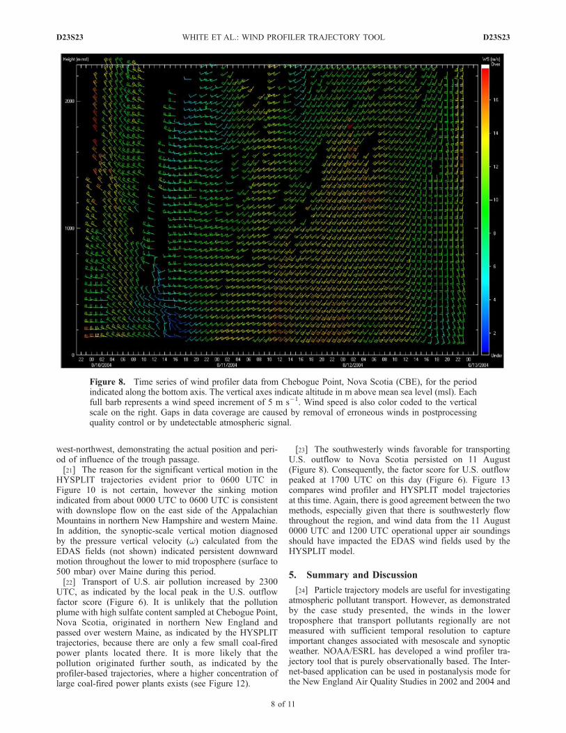
[23] The southwesterly winds favorable for transportingU.S. outflow to Nova Scotia persisted on 11 August(Figure 8). Consequently, the factor score for U.S. outflowpeaked at 1700 UTC on this day (Figure 6). Figure 13compares wind profiler and HYSPLIT model trajectoriesat this time. Again, there is good agreement between the twomethods, especially given that there is southwesterly flowthroughout the region, and wind data from the 11 August0000 UTC and 1200 UTC operational upper air soundingsshould have impacted the EDAS wind fields used by theHYSPLIT model.

5. Summary and Discussion

[24] Particle trajectory models are useful for investigatingatmospheric pollutant transport. However, as demonstratedby the case study presented, the winds in the lowertroposphere that transport pollutants regionally are notmeasured with sufficient temporal resolution to captureimportant changes associated with mesoscale and synopticweather. NOAA/ESRL has developed a wind profiler tra-jectory tool that is purely observationally based. The Inter-net-based application can be used in postanalysis mode forthe New England Air Quality Studies in 2002 and 2004 and

Figure 8. Time series of wind profiler data from Chebogue Point, Nova Scotia (CBE), for the periodindicated along the bottom axis. The vertical axes indicate altitude in m above mean sea level (msl). Eachfull barb represents a wind speed increment of 5 m s�1. Wind speed is also color coded to the verticalscale on the right. Gaps in data coverage are caused by removal of erroneous winds in postprocessingquality control or by undetectable atmospheric signal.


8 of 11

D23S23

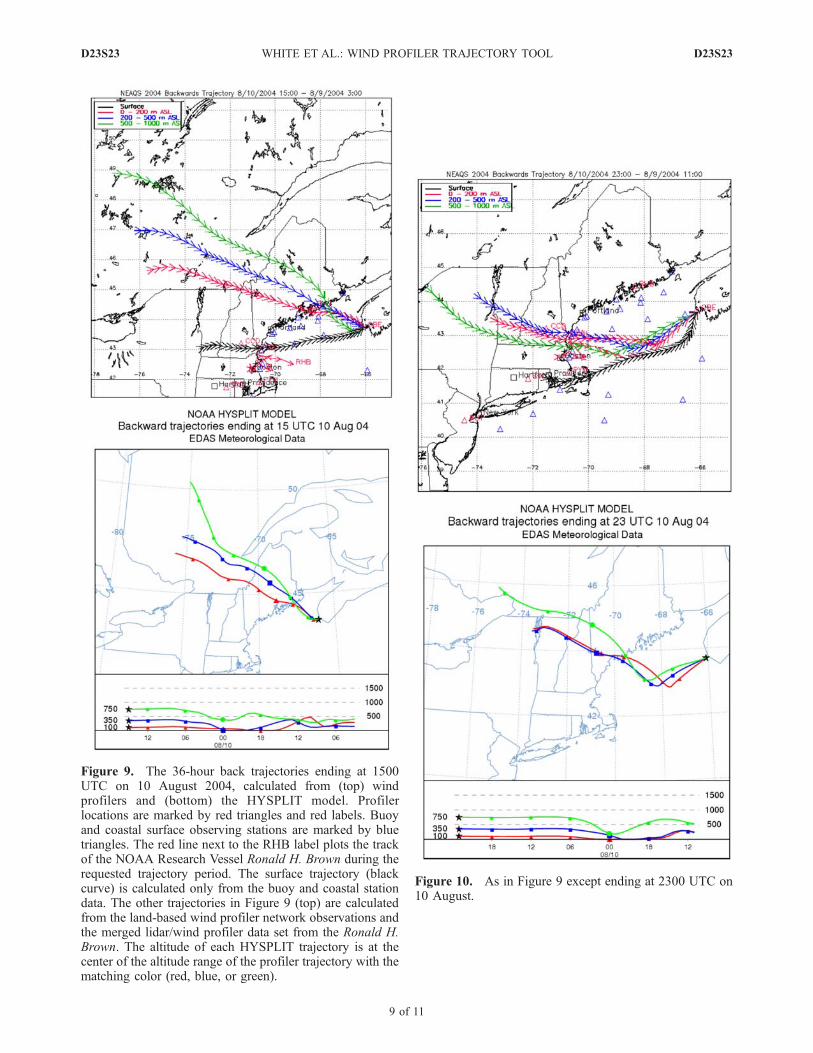
Figure 9. The 36-hour back trajectories ending at 1500UTC on 10 August 2004, calculated from (top) windprofilers and (bottom) the HYSPLIT model. Profilerlocations are marked by red triangles and red labels. Buoyand coastal surface observing stations are marked by bluetriangles. The red line next to the RHB label plots the trackof the NOAA Research Vessel Ronald H. Brown during therequested trajectory period. The surface trajectory (blackcurve) is calculated only from the buoy and coastal stationdata. The other trajectories in Figure 9 (top) are calculatedfrom the land-based wind profiler network observations andthe merged lidar/wind profiler data set from the Ronald H.Brown. The altitude of each HYSPLIT trajectory is at thecenter of the altitude range of the profiler trajectory with thematching color (red, blue, or green).

Figure 10. As in Figure 9 except ending at 2300 UTC on10 August.


9 of 11

D23S23

in real time, beginning in 2005, for the Texas Air QualityStudy. The wind fields for this tool are derived primarilyfrom networks of wind profilers that provide continuous,hourly, height-resolved observations of wind speed anddirection. Over the Gulf of Maine and the Gulf of Mexico,surface trajectories can be computed using surface obser-vations from NOAA and cooperative agency buoy andshoreline stations. The profiler trajectory tool complementsthe more sophisticated model trajectory tools that, for

Figure 11. Comparison of wind profiles produced bythe 40-km EDAS (E) and wind profiler network (P) from(a) Chebogue Point, Nova Scotia, and (b) the Gulf of Maineat 43�N and 68�W. Each full barb represents a wind speedincrement of 5.0 m s�1. The wind profiles from the profilernetwork were derived by combining the winds from theindividual profiler sites using an inverse distance-squaredweighting function (see text). The EDAS fields wereconverted from a pressure vertical coordinate to an altitudevertical coordinate using the 1976 Standard Atmosphere.

Figure 12. Distribution of coal-fired power plants in thenortheastern United States as of 2004. The size of the circlemarking the location of each plant denotes the range of theplant’s summer generating capacity in Megawatts (MW), asindicated by the key at the bottom left. Reprinted withpermission from Platts, a division of McGraw-Hill Compa-nies, Inc.

Figure 13. As in Figure 9 except ending at 1700 UTC on11 August.


10 of 11

D23S23

example, can be run automatically on a regular basis fortime receptor analysis or conceptual model development.[25] The backbone of the nation’s operational, all-weather,

upper air wind observing system is still the rawinsonde,which provides wind profiles throughout the atmosphericcolumn at 12-hour intervals. Unfortunately, the denseprofiler networks that provide continuous hourly windsfor documenting regional transport are generally onlyavailable in specialized research field campaigns, and thereis still work that needs to be done to improve real-timeinstrument performance, especially with regard to removinginterfering signals that lead to erroneous wind measure-ments (e.g., radio frequency interference, ground clutter,migrating birds). Once these problems are solved, it is ourhope that the observing gap for atmospheric transport willbe addressed in future upgrades to the nation’s upper airobserving system.

[26] Acknowledgments. We thank the dedicated engineering staffs inthe Physical and Chemical Sciences Divisions of NOAA/ESRL for install-ing and maintaining the NOAA profilers used in this study. We thank theindividual cooperative agency profiler operators and the Global SystemsDivision of NOAA/ESRL for providing cooperative agency profiler data.We thank Tom Shyka of the Gulf of Maine Ocean Observing System(GoMOOS) and the Physical Oceanography Group at the University ofMaine for providing the GoMOOS and NOOA buoy and C-MAN stationdata used in the New England trajectory tool. The critical review providedby J. W. Bao and two anonymous reviewers helped improve the manuscript.The air quality study wind profiler deployments and related research weresupported by the NOAA Health of the Atmosphere Program. We thankSusanne Hering and Nathan Kreisberg of Aerosol Dynamics for their workin developing and helping to deploy TAG. TAG measurements weresupported by a U.S. Department of Energy SBIR Phase I and II grant(DE-FG02-02ER83825) and a graduate research fellowship for BrentWilliams from DOE’s Global Change Education Program.

ReferencesAngevine, W. M. (1997), Errors in mean vertical velocities measured byboundary layer wind profilers, J. Atmos. Oceanic Technol., 14, 565–569.

Banta, R. M., et al. (1998), Daytime buildup and nighttime transport ofurban ozone in the boundary layer during a stagnation episode, J. Geo-phys. Res., 103(D17), 22,519–22,544.

Banta, R. M., C. J. Senff, J. Nielsen-Gammon, L. S. Darby, T. B. Ryerson,R. J. Alvarez, S. P. Sandberg, E. J. Williams, and M. Trainer (2005), Abad air day in Houston, Bull. Am. Meteorol. Soc., 86(5), 657–669,doi:10.1175/BAMS-86-5-657.

Browning, K. A., and R. Wexler (1968), The determination of kinematicproperties of a wind field using Doppler radar, J. Appl. Meteorol., 7,105–113.

Carter, D. A., K. S. Gage, W. L. Ecklund, W. M. Angevine, P. E. Johnston,A. C. Riddle, J. Wilson, and C. R. Williams (1995), Developments inUHF lower tropospheric wind profiling at NOAA’s Aeronomy Labora-tory, Radio Sci., 30, 977–1001.

Chadwick, R. B. (1988), The Wind Profiler Demonstration Network paperpresented at Symposium on Lower Tropospheric Profiling: Needs andTechnologies, Am. Meteorol. Soc., Boulder, Colo., 31 May to 3 June.

Ecklund, W. L., D. A. Carter, and B. B. Balsley (1979), Continuousmanagement of upper atmospheric winds and turbulence using a VHFDoppler radar: Preliminary results, J. Atmos. Terr. Phys., 41, 983–984.

Fehsenfeld, F. C., et al. (2006), International Consortium for AtmosphericResearch on Transport and Transformation (ICARTT): North America toEurope: Overview of the 2004 summer field study, J. Geophys. Res.,doi:10.1029/2006JD007829, in press.

Fisher, E., A. Pszenny, W. Keene, J. Maben, A. Smith, J. Stutz, R. Talbot,C. Senff, and A. White (2006), Nitric acid phase partitioning and cyclingin the New England coastal atmosphere, J. Geophys. Res., 111, D23S09,doi:10.1029/2006JD007328.

Frisch, A. S., B. L. Weber, R. G. Strauch, D. A. Merritt, and K. P. Moran(1986), The altitude coverage of the Colorado wind profilers at 50, 405,and 915 MHz, J. Atmos. Oceanic Technol., 3, 680–692.

Martner, B. E., D. B. Wuertz, B. B. Stankov, R. G. Strauch, E. R. Westwater,K. S. Gage, W. L. Ecklund, C. L. Martin, and W. F. Dabberdt (1993),An evaluation of wind profiler, RASS, and microwave radiometerperformance, Bull. Am. Meteorol. Soc., 74, 599–613.

McNider, R., W. B. Norris, A. J. Song, R. L. Clymer, S. Gupta, R. M.Banta, R. J. Zamora, A. B. White, and M. Trainer (1998), Meteorologicalconditions during the 1995 SOS Nashville/Middle Tennessee field inten-sive, J. Geophys. Res., 103(D17), 22,225–22,243.

Meagher, J. F., E. B. Cowling, F. C. Fehsenfeld, and W. J. Parkhurst (1998),Ozone formation and transport in southeastern United States: Overviewof the SOS Nashville/Middle Tennessee Ozone Study, J. Geophys. Res.,103(D17), 22,213–22,223.

Millet, D. B., et al. (2006), Chemical characteristics of North Americansurface layer outflow: Insights from Chebogue Point, Nova Scotia,J. Geophys. Res., 111, D23S53, doi:10.1029/2006JD007287.

Weber, B. L., D. B. Wuertz, D. C. Welsh, and R. McPeek (1993), Qualitycontrols for profiler measurements of winds and RASS temperatures,J. Atmos. Oceanic Technol., 10, 452–464.

White, A. B., et al. (2006), Comparing the impact of meteorologicalvariability on surface ozone during the NEAQS (2002) and ICARTT(2004) field campaigns, J. Geophys. Res., doi:10.1029/2006JD007590,in press.

Wolfe, D. W., et al. (2006), Shipboard multi-sensor wind profiles fromNEAQS 2004, J. Geophys. Res., doi:10.1029/2006JD007344, in press.

Worthington, R. M. (2002), Comment on ‘‘Comparison of radar reflectivityand vertical velocity observed with a scannable C-band radar and twoUHF profilers in the lower troposphere’’, J. Atmos. Oceanic Technol., 20,1221–1223.

��L. S. Darby and A. N. Keane, Earth System Research Laboratory,

NOAA, Boulder, CO 80305, USA.I. V. Djalalova, C. J. Senff, A. B. White, and D. E. White, Cooperative

Institute for Research in Environmental Sciences, University of Colorado,Boulder, CO 80309, USA. ([email protected])A. H. Goldstein and B. J. Williams, Department of Environmental

Science, Policy, and Management, University of California, Berkeley, CA94720, USA.D. C. Ruffieux, Aerological Station, MeteoSwiss, CH-1530 Payerne,

Switzerland.


11 of 11

D23S23

Documents

A wind profiler trajectory tool for air quality transport applications