Wavelet based methods for improved wind profiler signal processing

Annales Geophysicae (2001) 19: 825–836c© European Geophysical Society 2001Annales

Geophysicae

Wavelet based methods for improved wind profiler signal processing

V. Lehmann1 and G. Teschke2

1Deutscher Wetterdienst, Meteorologisches Observatorium Lindenberg, D-15864 Lindenberg, Germany2Zentrum fur Technomathematik, Universitat Bremen, D-28334 Bremen, Germany

Received: 8 August 2000 – Revised: 28 February 2001 – Accepted: 8 March 2001

Abstract. In this paper, we apply wavelet thresholding forremoving automatically ground and intermittent clutter (air-plane echoes) from wind profiler radar data. Using the con-cept of discrete multi-resolution analysis and non-parametricestimation theory, we develop wavelet domain thresholdingrules, which allow us to identify the coefficients relevant forclutter and to suppress them in order to obtain filtered recon-structions.

Key words. Meteorology and atmospheric dynamics (in-struments and techniques) – Radio science (remote sensing;signal processing)

1 Introduction

Radar Wind Profilers (RWP) are versatile tools used to rou-tinely probe the Earth’s atmosphere. This technology origi-nally developed for studying the dynamics of the middle at-mosphere in the seventies (Hardy and Gage, 1990) is, mean-while, very prominent in the meteorological research com-munity. Meteorological services started using these systemsoperationally within the Global Observing System (GOS)(see Monna and Chadwick (1998)).

Most of these RWP employ the Doppler-beam swinging(DBS) method for the determination of the vertical profile ofthe horizontal wind and, under certain conditions, the verticalwind component. These radars transmit short electromag-netic pulses in a fixed beam direction and sample the smallfraction of the electromagnetic field backscattered to the an-tenna. At least three linear independent beam directions arerequired to transform the measured ’line-of-sight’ radial ve-locities into the wind vector. Due to the nature of the act-ing atmospheric scattering processes, the received signal isseveral orders of magnitude weaker than the transmitted sig-nal. The received signal is Doppler shifted, which is usedto determine the velocity component of “the atmosphere”projected onto the beam direction. As the bandwidthB of

Correspondence to:V. Lehmann ([email protected])

a transmitted electromagnetic pulse of durationτ is muchlarger (B ∝ 1/τ ≈ 100...1000 kHz) than the Doppler shift(fd ≈ 10...500 Hz), the frequency shift cannot be deter-mined from the processing of a single pulse. Instead, the re-turn of many pulses is evaluated to compute the Doppler fre-quency from the slowly changing phase of the received sig-nals (Burgess and Ray, 1986). Sampling is done after the re-ceivers quadrature detector (for the in-phase and quadrature-phase components of the signal) using sample and hold cir-cuits prior to the A/D conversion. The sampling rate is deter-mined by the pulse repetition periodT . The samples at eachrange gate form a discrete complex time series, which is theraw dataof the measurement at this gate. The following digi-tal signal processing has the purpose of extracting the desiredatmospheric information from the radar echoes. More de-tails about coherent radar technology and in particular, windprofilers, can be found in standard textbooks (Gossard andStrauch, 1983; Doviak and Zrnic, 1993) and in several re-view papers, e.g. Rottger and Larsen (1990).

In this paper, we propose a modified signal processingtechnique for RWPs. It must be noted that signal processingincludes all operations that are performed on the radar signal,i.e. analog1 as well as digital processing2. However, in thefollowing, we will only concentrate on digital signal process-ing. The incredible development of fast digital processorsopens up new opportunities to optimize this latter part of thesignal processing chain. The goals of signal processing, assummarized by Keeler and Passarelli (1990), are:

– to provide accurate, unbiased estimates of the character-istics of the desired atmospheric echoes;

– to estimate the confidence/accuracy of the measurement;

– to mitigate effects of interfering signals;

– to reduce the data rate.

1amplification, mixing and matched filtering2after A/D conversion

826 V. Lehmann and G. Teschke: Wavelet based methods for improved wind profiler signal processing

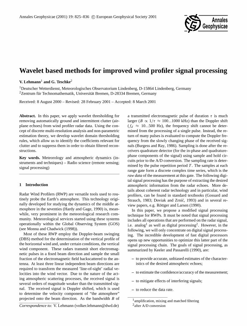
Range-gated and digitized received Signal

↓

Coherent Integration (Time-Domain Averaging)

↓

Fourier Analysis (Spectral Averaging)

↓

Spectral Parameter Estimation (Moments)

↓

Wind Estimation

Fig. 1. The figure shows the flow diagram of ’classical’ digital sig-nal processing.

The fundamental base parameters of the atmospheric sig-nal are the reflected power, the radial velocity and the veloc-ity variance (e.g. the first three moments of the Doppler spec-trum). Signal processing ends with the estimation of the mo-ments of the Doppler spectrum and further data processing isthen performed to finally determine the wind and other me-teorological parameters using measurements from all radarbeams. This distinction, which goes back originally to Keelerand Passarelli (1990), has become more and more blurred,since some modern algorithms make use of the moments ofthe Doppler spectrum with the help of continuity and otherinformation (Wilfong et al., 1999b). However, we will referhere to the usually applied and well established “classical”signal processing, as described by Tsuda (1989), Rottger andLarsen (1990), among others.

2 Statement of the problem

Before we discuss the problems that are associated with the“classical” processing, let us briefly repeat the steps as visu-alized in Fig. 1. In particular, we refer to the signal process-ing as it is implemented in the RWP, whose data are used inthis study.

Digital signal processing in a system using an analog re-ceiver3 starts with the sampling of the in- and quadrature-phase components of the received signal at a rate that is de-termined by the pulse repetition periodT . To reduce the datarate for further processing, hardware adder circuits performa so-called coherent integration (Barth et al., 1994; Carteret al., 1995; Wilfong et al., 1999a), adding someN (typi-cally ten to hundred) complex samples together. Mathemati-cally, this operation can be seen as a combination of a digitalboxcar filtering, followed by an undersampling at a rate ofNT (Schmidt et al., 1979; Farley, 1985). If the radar systemuses pulse compression techniques (e.g. phase coding using

3For future systems, digital receivers will slightly change thesignal processing but this has no consequence here.

complementary sequences), then the next step is decoding(Schmidt et al., 1979; Sulzer and Woodman, 1984; Farley,1985; Ghebrebrhan and Crochet, 1992; Spano and Ghebre-brhan, 1996). The coherently averaged and decoded samplesare then used to compute the Doppler spectrum using theWindowed Fourier Transform (FFT) and the Periodogrammethod (see Keeler and Passarelli, 1990). In our system, aFourier transformed Hanning-window is convolved with theresult of the FFT. A number (typically some ten) of individ-ual Doppler spectra is then incoherently averaged to improvethe detectability of the signal (Tsuda, 1989, see). Finally, thenoise level is estimated with the method proposed by Hilde-brand and Sekhon (1974), and the moments of the maximumsignal in the spectrum are computed over the range where thesignal is above the noise level (May and Strauch, 1989).

The problem with this type of signal processing is the un-derlying assumption that the signal consists of only two parts:the signal, that is produced by one atmospheric scatteringprocess, and noise (different sources, mainly thermal elec-tronic noise and cosmic noise). This is certainly not true,especially at UHF, where the desired atmospheric signal it-self is often the result of two distinct scattering processes,namely scattering at inhomogenities of the refractive index(Bragg scattering) and scattering at particles, such as dropletsor ice crystals (Rayleigh scattering) (see, for instance, Gos-sard, 1979; Gossard and Strauch, 1981, 1983; Ralph et al.,1995, 1996; Gage et al., 1999). Therefore, even the desiredatmospheric signal may have different characteristics. But,as experience shows us, the most serious problems are causedby the following contributions to the signal:

Ground Clutter. Echo returns from the ground surrounding the site,which emerge from antenna’s sidelobes;

Intermittent Clutter. Returns from unwanted targets, such as air-planes or birds, from both the antenna’ss main lobe and the side-lobes;

Radio Frequency Interference (RFI). RFI can emerge from exter-nal radio-frequency transmissions within the passband of the re-ceiver (matched filter), or it can be generated internally due to im-perfections of the radar hardware.

Recently, much work has and continues to be done to de-velop frequency domain processing algorithms, i.e. to im-prove the process of moment estimation. The purpose ofthese methods is to select the “true” atmospheric signal inthe Doppler spectrum even in the presence of severe contam-ination. Only this signal will then be used for the determina-tion of the wind vector. Several criteria are used to make an“intelligent” selection of the signal (Clothiaux et al., 1994;Gossard, 1997; Griesser, 1998; Cornman et al., 1998; Schu-mann et al., 1999; Wilfong et al., 1999b; Morse et al., 2000).The emphasis on frequency domain processing was probablycaused by the fact that it is much easier to handle spectraldata, as the data volume is significantly reduced due to thedata compression effect of the periodogram computation andthe spectral integration. Some of these “multiple moment es-timation” algorithms additionally assign a quality indicator

V. Lehmann and G. Teschke: Wavelet based methods for improved wind profiler signal processing 827

to the computed wind values, which does not only dependson the quality of the moment estimation, but also uses con-tinuity criteria (Wilfong et al., 1999b) and the testing of as-sumptions that are inherent to the DBS method (Goodrichet al., 2000). First evaluations have indeed shown a verypromising improvement of those new algorithms (Cohn et al.,2000), but no long-term evaluation against independent mea-surement systems, such as the Rawinsonde, has been per-formed so far.

Modified time domain processing has been proposed toreduce the problems caused by contaminating signals. Oneproblem emerges from the fact that the receiver filter of theradar is matched to the transmitted pulse in order to optimizethe single pulse signal-to-noise ratio for improved signal de-tection in the presence of noise (Tsuda, 1989; Papoulis, 1991;Doviak and Zrnic, 1993). This implies a receiver bandwidthof B ∝ 1/τ . Yet, the sampling is done at a rate ofT (with-out coherent averaging) or evenNT (with coherent averag-ing). Thus, the Nyquist frequency, after coherent averaging,is severely smaller than the frequency that a received signalmight have. Of course, it is true that the desired atmosphericsignal is band-limited by a sufficiently long coherence timeof the scattering process, so that this undersampling has noconsequences (aside from some modification due to the fil-tering characteristics of the coherent integration). If there is,however, some artificial signal, such as RFI present, whosespectrum falls into the receiver passband, the complex I/Q-timeseries then represents a process that is only band-limitedby the receiver hardware. The consequence of undersam-pling is frequency aliasing of higher frequency componentsinto the atmospheric band of interest. This problem is espe-cially critical in the U.S., where profilers at 449 MHz operatesimultaneously with amateur radios. Although the problemof principal undersampling cannot be solved due to the factthat 1/τ � 1/T , Wilfong et al. (1999a) achieved an im-proved time domain filtering using a four-term Blackman-Harris filter (Harris, 1978), instead of the usually appliedboxcar filter of coherent averaging. While this kind of digitalfiltering helps to reject RFI, it is not helpful in the presenceof ground and intermittent clutter. Those clutter signals fallwell into the region of the desired atmospheric signal. Mayand Strauch (1998) proposed the use of linear convolutionfilters (digital FIR4 filters) with a band rejection characteris-tic around zero Doppler shift (DC). This requires, however,a long filter sequence and also does not protect against in-termittent clutter signals, which can occur at any frequency.Additionally, the transfer characteristic is fixed for a set ofgiven filter coefficients. For that reason, wavelet domain fil-tering of ground and intermittent clutter (Jordan et al., 1997;Boisse et al., 1999) has been proposed. The main purposeof all these time domain operations is the filtering aspect,i.e. the intention is to “clean” the raw data from contami-nating signals while leaving the desired atmospheric contri-bution ideally intact. In the following, we will concentrateon the clutter problem and investigate the properties of these

4Finite Impulse Response

Table 1. Technical specification of RWP and radar operating pa-rameters

Site name Lindenberg482 MHz Profiler

Latitude 52.21 NLongitude 14.13 EAltitude 101 m mslFrequency 482.0078 MHzOne-way beamwidth 3 degreesNumber of beams 5Zenith distance (oblique beams) 15 degreesEffective antenna area 140 m2

Pulse peak power 16 kWAltitude Range 0.5–8.0 km

(Low Mode)Beamdirection during raw data sampling East

(Azimuth: 79 Elev. 75)InterPulsePeriod (T) 61µsPulsewidth (τ ) 1700 ns (Low Mode)Delay to first gate 4800 nsGate Spacing 1700 nsNumber of gates 30# of coherent integrations (N) 144# of spectral integrations 1 (none)# of points in online FFT 2048System Delay (w/ 1700 ns pulse) 1550 ns

signals and the possibility of applying nonlinear wavelet fil-ters. There are not many investigations about the propertiesof RWP raw data. Normally, using statistical arguments, oneassumes simply a Gaussian signal characteristic for atmo-spheric and clutter signals, as well as for noise (Doviak andZrnic, 1993; Petitdidier et al., 1997). Recently, Muschin-ski et al. (1999) used data from a large-eddy simulation toderive I/Q signals for clear air scattering, and Capsoni andD’Amico (1998) presented a software-based radar simulatorfor generating time series from a synthetic distribution of hy-drometeors. For our purpose, we assume that the Gaussianmodel describes sufficiently well both the atmospheric scat-tering component and the ground clutter signal. Intermittentclutter returns can be described by the simple model givenby Boisse et al. (1999), with their main property being thetransient character.

The 482 MHz wind profiler, whose data are used in thisstudy, was installed at the Meteorological Observatory Lin-denberg during the summer of 1996. The system is the pro-totype for three additional profilers to be installed in Ger-many in the future to supplement the operational aerologicalnetwork of the Deutscher Wetterdienst (DWD). A summaryof the main characteristics of the system is given in Table1. For a more detailed description, the reader is referredto Steinhagen et al. (1998). The system is operated quasicontinuously using a five beam configuration. All the mainsystem parameters can be freely programmed which easesspecial investigations, such as the investigation of the detri-mental ground clutter signal that was present in the system’s


Northerly Wind

Calm

< 1.25 m/s

2.50 m/s

5.00 m/s

7.50 m/s

10.00 m/s

15.00 m/s

17.50 m/s

22.50 m/s

25.00 m/s

35.00 m/s

37.50 m/s

50.00 m/s

DWD-TWP Profiler DataLindenberg, Germany (TWP) Date: 11/30/99 - 12/1/99

Elev. (m): 103

WS (m/s)

Time (UTC)

Height(m-agl)

Validation Level: 0.5Printed: 12/2/99

20

30

40

50

Under

Over

17 18 19 20 21 22 23 0012/1/99

01 02 03 04 05 06 07 08 09 10 11 12 13 14 15 160

1000

2000

3000

4000

5000

6000

7000

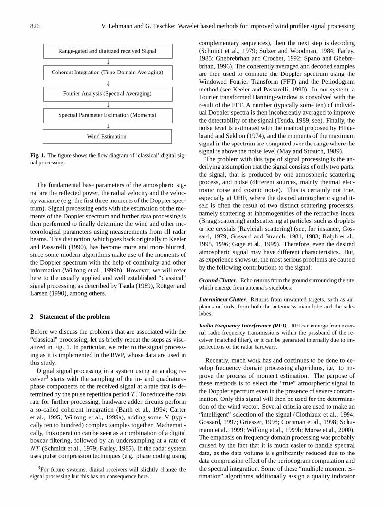
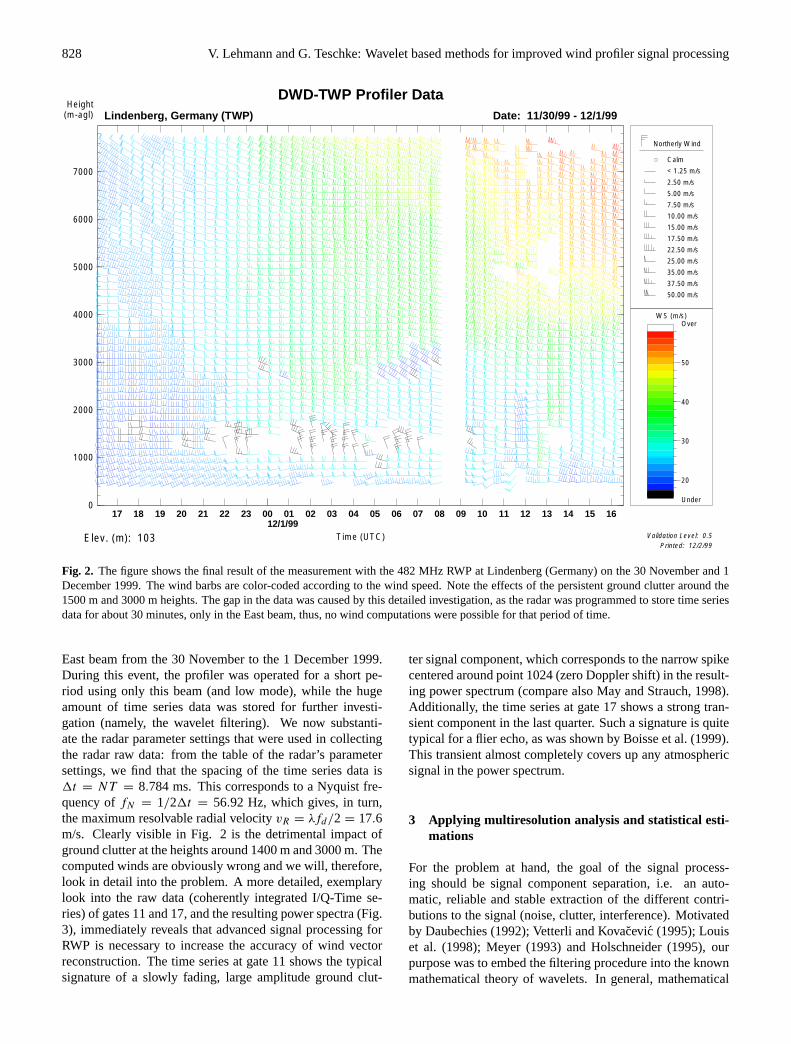
Fig. 2. The figure shows the final result of the measurement with the 482 MHz RWP at Lindenberg (Germany) on the 30 November and 1December 1999. The wind barbs are color-coded according to the wind speed. Note the effects of the persistent ground clutter around the1500 m and 3000 m heights. The gap in the data was caused by this detailed investigation, as the radar was programmed to store time seriesdata for about 30 minutes, only in the East beam, thus, no wind computations were possible for that period of time.

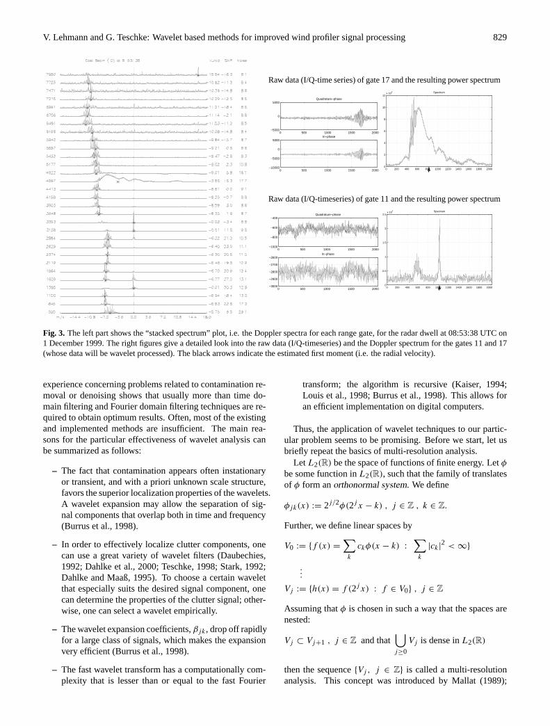
East beam from the 30 November to the 1 December 1999.During this event, the profiler was operated for a short pe-riod using only this beam (and low mode), while the hugeamount of time series data was stored for further investi-gation (namely, the wavelet filtering). We now substanti-ate the radar parameter settings that were used in collectingthe radar raw data: from the table of the radar’s parametersettings, we find that the spacing of the time series data is1t = NT = 8.784 ms. This corresponds to a Nyquist fre-quency offN = 1/21t = 56.92 Hz, which gives, in turn,the maximum resolvable radial velocityvR = λfd/2 = 17.6m/s. Clearly visible in Fig. 2 is the detrimental impact ofground clutter at the heights around 1400 m and 3000 m. Thecomputed winds are obviously wrong and we will, therefore,look in detail into the problem. A more detailed, exemplarylook into the raw data (coherently integrated I/Q-Time se-ries) of gates 11 and 17, and the resulting power spectra (Fig.3), immediately reveals that advanced signal processing forRWP is necessary to increase the accuracy of wind vectorreconstruction. The time series at gate 11 shows the typicalsignature of a slowly fading, large amplitude ground clut-

ter signal component, which corresponds to the narrow spikecentered around point 1024 (zero Doppler shift) in the result-ing power spectrum (compare also May and Strauch, 1998).Additionally, the time series at gate 17 shows a strong tran-sient component in the last quarter. Such a signature is quitetypical for a flier echo, as was shown by Boisse et al. (1999).This transient almost completely covers up any atmosphericsignal in the power spectrum.

3 Applying multiresolution analysis and statistical esti-mations

For the problem at hand, the goal of the signal process-ing should be signal component separation, i.e. an auto-matic, reliable and stable extraction of the different contri-butions to the signal (noise, clutter, interference). Motivatedby Daubechies (1992); Vetterli and Kovacevic (1995); Louiset al. (1998); Meyer (1993) and Holschneider (1995), ourpurpose was to embed the filtering procedure into the knownmathematical theory of wavelets. In general, mathematical


Raw data (I/Q-time series) of gate 17 and the resulting power spectrum

0 500 1000 1500 2000−5000

0

5000Quadrature−phase

0 500 1000 1500 2000−10000

−5000

0

5000In−phase

0 200 400 600 800 1000 1200 1400 1600 1800 20000

2

4

6

8

10

12x 10

4 Spectrum

Raw data (I/Q-timeseries) of gate 11 and the resulting power spectrum

0 500 1000 1500 2000−1000

−800

−600

−400Quadrature−phase

0 500 1000 1500 2000−3000

−2900

−2800

−2700

−2600In−phase

0 200 400 600 800 1000 1200 1400 1600 1800 20000

0.5

1

1.5

2

2.5x 10

4 Spectrum

Fig. 3. The left part shows the “stacked spectrum” plot, i.e. the Doppler spectra for each range gate, for the radar dwell at 08:53:38 UTC on1 December 1999. The right figures give a detailed look into the raw data (I/Q-timeseries) and the Doppler spectrum for the gates 11 and 17(whose data will be wavelet processed). The black arrows indicate the estimated first moment (i.e. the radial velocity).

experience concerning problems related to contamination re-moval or denoising shows that usually more than time do-main filtering and Fourier domain filtering techniques are re-quired to obtain optimum results. Often, most of the existingand implemented methods are insufficient. The main rea-sons for the particular effectiveness of wavelet analysis canbe summarized as follows:

– The fact that contamination appears often instationaryor transient, and with a priori unknown scale structure,favors the superior localization properties of the wavelets.A wavelet expansion may allow the separation of sig-nal components that overlap both in time and frequency(Burrus et al., 1998).

– In order to effectively localize clutter components, onecan use a great variety of wavelet filters (Daubechies,1992; Dahlke et al., 2000; Teschke, 1998; Stark, 1992;Dahlke and Maaß, 1995). To choose a certain waveletthat especially suits the desired signal component, onecan determine the properties of the clutter signal; other-wise, one can select a wavelet empirically.

– The wavelet expansion coefficients,βjk, drop off rapidlyfor a large class of signals, which makes the expansionvery efficient (Burrus et al., 1998).

– The fast wavelet transform has a computationally com-plexity that is lesser than or equal to the fast Fourier

transform; the algorithm is recursive (Kaiser, 1994;Louis et al., 1998; Burrus et al., 1998). This allows foran efficient implementation on digital computers.

Thus, the application of wavelet techniques to our partic-ular problem seems to be promising. Before we start, let usbriefly repeat the basics of multi-resolution analysis.

LetL2(R) be the space of functions of finite energy. Letφ

be some function inL2(R), such that the family of translatesof φ form anorthonormal system. We define

φjk(x) := 2j/2φ(2jx − k) , j ∈ Z , k ∈ Z.

Further, we define linear spaces by

V0 := {f (x) =

∑k

ckφ(x − k) :

∑k

|ck|2 < ∞}

...

Vj := {h(x) = f (2jx) : f ∈ V0} , j ∈ Z

Assuming thatφ is chosen in such a way that the spaces arenested:

Vj ⊂ Vj+1 , j ∈ Z and that⋃j≥0

Vj is dense inL2(R)

then the sequence{Vj , j ∈ Z} is called a multi-resolutionanalysis. This concept was introduced by Mallat (1989);


Meyer (1993).φ is called the father wavelet. Furthermore,one may define subspacesWj by

Vj+1 := Vj ⊕Wj

and iterating this we have⋃Vj = V0 ⊕

⊕j

Wj andL2(R) = V0 ⊕

⊕j

Wj .

Assuming that our data may be described by somef ∈ L2(R),we can represent the signal as a series

f (x) =

∑k

αkφ0k(x)+

∑j

∑k

βjkψjk(x),

where{ψjk}, k ∈ Z is an orthonormal basis inWj . Thefunctionψ is called mother wavelet.

This expansion is a special kind of orthogonal series.Hence, it would be useful to search in the framework ofnonparametric statistical estimation theory for an applicablemethod to solve our problem (Donoho and Johnstone, 1992).In case of orthogonal series estimation, the idea of recon-structing the desired atmospheric signal is simple. Basically,we replace the unknown wavelet coefficients in the waveletexpansion by estimates which are based on observed data.For that, we need a selection procedure to choose relevantcoefficients since the main emphasis of performing waveletdomain filtering is to create a suitable, i.e. problem matched,coefficient selecting procedure. To separate the atmosphericsignal component, we apply statistical estimation theory. Aside effect of using statistics is to obtain a measure of recon-struction quality. A typical quality measure is a loss func-tion/estimation error. Minimizing the error function revealsan objective evaluation and a self-acting filter algorithm.

The following sub-section describes the construction ofour atmospheric-signal-estimator. In advance, we briefly re-mark that in the following section, we assume that our sig-nal belongs to some Besov space, i.e. a generalized math-ematical function space. One special example is the pre-viously introduced function spaceL2(R). But sometimesit makes more sense to suppose that the derivatives of oursignal are of finite energy as well. In this and other situa-tions, the framework of Besov spaces is an adequate mathe-matical tool for our application. A Besov space, denoted byBspq , depends on three parameters:s smoothness, the num-ber of bounded derivatives andp, q which describe the un-derlying function spaceLq(lp). In the following, we makeuse of some well-known facts of estimation theory, whichare valid for almost all Besov spaces (Donoho and John-stone, 1992; Donoho et al., 1993; Johnstone and Silverman,1995; v. Sachs and MacGibbon, 1998; Dahlhaus et al., 1998;Hardle et al., 1998). If our signal is an element of one ofthese spaces (which is true for all practical signals), we canadapt wavelet threshold estimators. The main advantage ofthis framework is that we can use existing rules for evaluatingbounds and rates of convergence for our loss function, whichdescribes the quality of our reconstructed atmospheric signalcomponent. By optimizing bounds and rates of convergence,we obtain self acting algorithms.

For our purpose, we only need the following characteriza-tion of Besov spaces: A functionf belongs toBspq if

J spq(f ) = ‖α.‖lp +

(∑j≥0

(2j (s+1/2−1/p)‖βj.‖lp )

q

)1/q

< ∞.

We are looking for optimal reconstructions of functions be-longing to some subsetF spq(M) = {f ∈ Bspq : J spq < M}.For our calculations, we assume that the function is inL2(R)ands is small.

From given measurements(Y1, . . . , Yn), we want to esti-mate the functionf in the simple model

Yi = f (Xi)+ εi .

We assume that we have theXi on a regular grid andε isa random variable (a stochastic process which describes allnon-atmospheric components). The basic idea is to replacethe wavelet coefficients in the series expansion by empiricalestimates

αk =1

n

n∑i=1

Yi · ϕ0k(Xi) and βjk =1

n

n∑i=1

Yi · ψjk(Xi),

where theXi are time stamps and theYi are observations. Astraightforward linear estimation is given by the projectiononto a subspaceVj1

fj1(x) =

∑k

αkϕ0k(x)+

j1∑j=0

∑k

βjkψjk(x).

To appraise this estimator, it is known that one may mea-sure the expected loss or the risk (inL2 sense)E‖fj1 − f ‖

22.

This measure is the so-called MISE (mean integrated squarederror). To determine the MISE, one may decompose it intoE‖fj1 −Efj1‖

22 (stochastic contribution) andE‖Efj1 −f ‖

22

(deterministic contribution). Under certain conditions, onemay find bounds for MISE:

supF s22(M)

‖Efj1 − f ‖2 ≤ C12−j1s

and

E‖fj1 − Efj1‖22 ≤ C2

2j1+1

n

and hence,

supf∈F s22(M)

E‖fj1 − f ‖22 ≤ C3

2j1

n+ C42−j1s .

A minimum of the sum is given by

supf∈F s22(M)

E‖fj1 − f ‖22 ≤ C5n

−2s/(2s+1),

furthermore, one can generalize this result forp > 2

supf∈F spq (M)

E‖fj1 − f ‖pp ≤ C5n

−ps/(2s+1).


This gives us an upper bound for the maximum risk. Thisbound becomes small if the number of observation increasesand if j1(n) is determined in such a way that the bias andstochastic bound are balanced (for detailed computations ofbounds, see v. Sachs and MacGibbon, 1998; Donoho et al.,1993; Donoho and Johnstone, 1992; Dahlhaus et al., 1998).

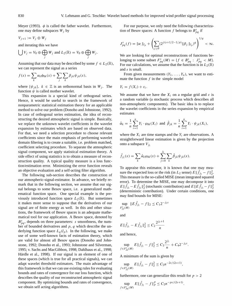
Obviously, this kind of linear estimation includes oscillat-ing components, in particular, the clutter components. Thisphenomenon occurs because we have taken the whole set ofwavelet coefficients up to scalej1, i.e. we have not per-formed any filtering step thus far. In the following, we needa suitable selection procedure for the coefficients in order toperform the necessary filtering step. We apply a so-calledhard thresholding and soft thresholding, respectively. Thismethodology was introduced and adapted to several prob-lems by Donoho and Johnstone (1992); Donoho et al. (1993).It is based on taking the discrete wavelet transform (usinga multiresolution analysis), passing the transform througha threshold (actually, the expansion coefficients are thresh-olded) and then taking the inverse DWT to obtain a filteredreconstruction. Note that this type of thresholding is usuallyapplied in a different way, by removing coefficientsbelowa certain threshold in order to “de-noise” the data (Burruset al., 1998, see Fig. 4). The functions for hard and softthresholding are defined by

θh(u) :=

{u, |u| ≥ λ

0, |u| < λ, θ s(u) :=

{(u−

λu|u|), |u| ≥ λ

0, |u| < λ

and the modified functions used here for hard and soft thresh-olding are given by the ruleη∗(u) = u− θ∗(u):

ηh(u) =

{u, |u| < λ

0, |u| ≥ λ, ηs(u) =

{u, |u| < λ

λ u|u|, |u| ≥ λ

.

Here,λ is an adequate threshold. Applying this rule to ourlinear wavelet estimator, we obtain a nonlinear estimator

f ∗(x) =

∑k

η∗(αk)ϕ0k(x)+

j1∑j=j0

∑k

η∗(βjk)ψjk(x),

whereη∗ is ηs or ηh, respectively.If the thresholdλ is specified according to the asymptotic

distribution of the empirical coefficients, then only those co-efficients remain which are supposed to carry significant sig-nal information. These are finally used for the reconstruc-tion by the inverse wavelet transform. For the correct levelof significance, an appropriate choice of the thresholdλ isneeded. In general, this does not only depend on the sam-ple sizen, but also on the resolution scalej , and locationk of the coefficients. In the case of regression with non-stationary errors, we have to use both a level and locationdependent threshold rule (v. Sachs and MacGibbon, 1998).The resulting non-linear estimator does not only provide lo-cal smoothers, but, in many situations, achieves the near-minimaxL2-rate for the risk of estimation, i.e. v. Sachs andMacGibbon (1998) for (random) thresholdsλjk satisfying

−2 −1 0 1 2−2

−1

0

1

2soft thresholding, λ=1

θs (u)

u−2 −1 0 1 2

−2

−1

0

1

2modified soft thresholding, λ=1

ηs (u)

u

−2 −1 0 1 2−2

−1

0

1

2hard thresholding, λ=1

θh (u)

u−2 −1 0 1 2

−2

−1

0

1

2modified hard thresholding, λ=1

ηh (u)

u

Fig. 4. This figure shows hard and soft thresholding.

σjk√

2 logMj ≤ λjk ≤ C

√lognn

for any positive constantC:

supf∈F s22(M)

E‖f ∗− f ‖

22 = O

((log(n)/n)2s/(2s+1)

),

whereσjk is the variance andMj denotes the number ofthe coefficients used in the nonlinear estimator. The opti-mal threshold rate(1/n)2s/(2s+1) is attained only for the idealthreshold. However, in practice, this is unknown. Therefore,we have to replaceσjk by some estimationσjk, which resultsin random thresholdsλjk = σjk

√2 logMj . Hence, the log-

term has to be understood as the price for some data-driventhreshold rule, and it originates due to the estimation of theunknown varianceσ 2

jk = Var(βjk).We conclude that we may adapt an estimation rule for our

desired atmospheric signal component where the quality ismeasurable in the sense ofL2-risk. This means the procedureused displays bounds for our reconstruction, and we may eas-ily determine the rate of convergence. The calculation of thewavelet coefficients can be done by using the fast waveletalgorithm which is easily implemented.

4 Removing clutter

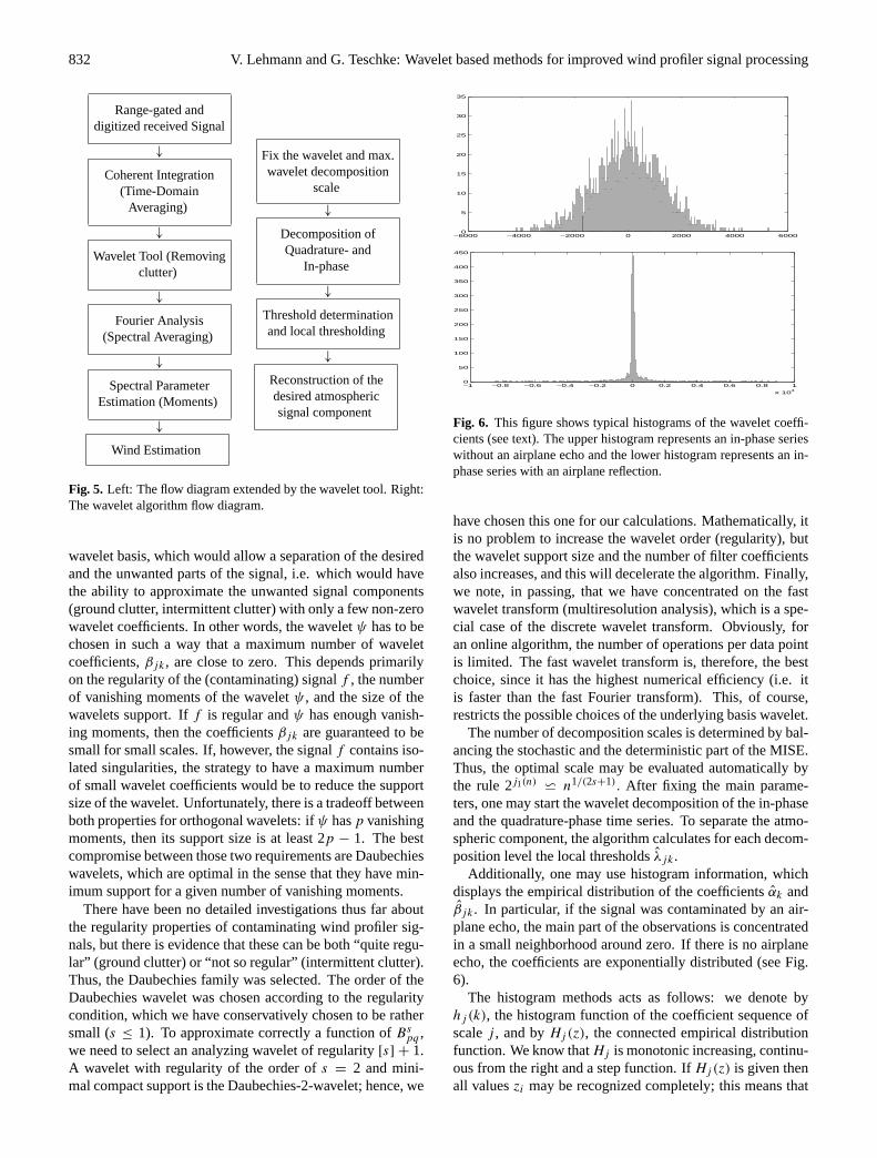
In this section, we will demonstrate the performance of non-linear wavelet filtering. This is done both with simulated andwith real data. For a better understanding, we particularizeFig. 1 to see where we have inserted the wavelet tool. Toapply our procedure, a more substantiated algorithm flow di-agram is shown in Fig. 5.

Following the first box in the algorithm flow diagram, onehas first to determine the analyzing wavelet (high and lowpass filter coefficients). Usually, the decomposition of a sig-nal in a basis (i.e. a wavelet series) has the goal of highlight-ing particular properties of the signal (Mallat, 1999). In theproblem of wind profiler signal filtering, the desired atmo-spheric signal component can be contaminated with spurioussignal components. The ultimate goal is obviously to find a


Range-gated anddigitized received Signal

↓

Coherent Integration(Time-Domain

Averaging)

↓

Wavelet Tool (Removingclutter)

↓

Fourier Analysis(Spectral Averaging)

↓

Spectral ParameterEstimation (Moments)

↓

Wind Estimation

Fix the wavelet and max.wavelet decomposition

scale

↓

Decomposition ofQuadrature- and

In-phase

↓

Threshold determinationand local thresholding

↓

Reconstruction of thedesired atmosphericsignal component

Fig. 5. Left: The flow diagram extended by the wavelet tool. Right:The wavelet algorithm flow diagram.

wavelet basis, which would allow a separation of the desiredand the unwanted parts of the signal, i.e. which would havethe ability to approximate the unwanted signal components(ground clutter, intermittent clutter) with only a few non-zerowavelet coefficients. In other words, the waveletψ has to bechosen in such a way that a maximum number of waveletcoefficients,βjk, are close to zero. This depends primarilyon the regularity of the (contaminating) signalf , the numberof vanishing moments of the waveletψ , and the size of thewavelets support. Iff is regular andψ has enough vanish-ing moments, then the coefficientsβjk are guaranteed to besmall for small scales. If, however, the signalf contains iso-lated singularities, the strategy to have a maximum numberof small wavelet coefficients would be to reduce the supportsize of the wavelet. Unfortunately, there is a tradeoff betweenboth properties for orthogonal wavelets: ifψ hasp vanishingmoments, then its support size is at least 2p − 1. The bestcompromise between those two requirements are Daubechieswavelets, which are optimal in the sense that they have min-imum support for a given number of vanishing moments.

There have been no detailed investigations thus far aboutthe regularity properties of contaminating wind profiler sig-nals, but there is evidence that these can be both “quite regu-lar” (ground clutter) or “not so regular” (intermittent clutter).Thus, the Daubechies family was selected. The order of theDaubechies wavelet was chosen according to the regularitycondition, which we have conservatively chosen to be rathersmall (s ≤ 1). To approximate correctly a function ofBspq ,we need to select an analyzing wavelet of regularity[s] + 1.A wavelet with regularity of the order ofs = 2 and mini-mal compact support is the Daubechies-2-wavelet; hence, we

−6000 −4000 −2000 0 2000 4000 60000

5

10

15

20

25

30

35

−1 −0.8 −0.6 −0.4 −0.2 0 0.2 0.4 0.6 0.8 1

x 104

0

50

100

150

200

250

300

350

400

450

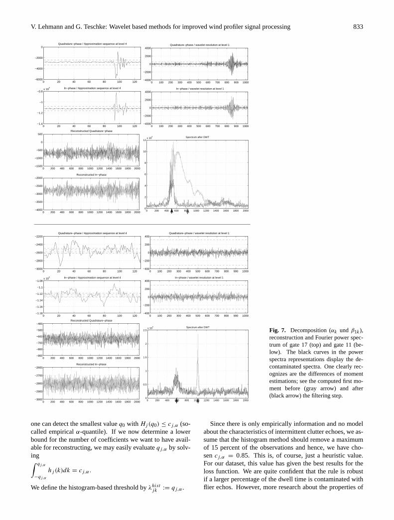
Fig. 6. This figure shows typical histograms of the wavelet coeffi-cients (see text). The upper histogram represents an in-phase serieswithout an airplane echo and the lower histogram represents an in-phase series with an airplane reflection.

have chosen this one for our calculations. Mathematically, itis no problem to increase the wavelet order (regularity), butthe wavelet support size and the number of filter coefficientsalso increases, and this will decelerate the algorithm. Finally,we note, in passing, that we have concentrated on the fastwavelet transform (multiresolution analysis), which is a spe-cial case of the discrete wavelet transform. Obviously, foran online algorithm, the number of operations per data pointis limited. The fast wavelet transform is, therefore, the bestchoice, since it has the highest numerical efficiency (i.e. itis faster than the fast Fourier transform). This, of course,restricts the possible choices of the underlying basis wavelet.

The number of decomposition scales is determined by bal-ancing the stochastic and the deterministic part of the MISE.Thus, the optimal scale may be evaluated automatically bythe rule 2j1(n) w n1/(2s+1). After fixing the main parame-ters, one may start the wavelet decomposition of the in-phaseand the quadrature-phase time series. To separate the atmo-spheric component, the algorithm calculates for each decom-position level the local thresholdsλjk.

Additionally, one may use histogram information, whichdisplays the empirical distribution of the coefficientsαk andβjk. In particular, if the signal was contaminated by an air-plane echo, the main part of the observations is concentratedin a small neighborhood around zero. If there is no airplaneecho, the coefficients are exponentially distributed (see Fig.6).

The histogram methods acts as follows: we denote byhj (k), the histogram function of the coefficient sequence ofscalej , and byHj (z), the connected empirical distributionfunction. We know thatHj is monotonic increasing, continu-ous from the right and a step function. IfHj (z) is given thenall valueszi may be recognized completely; this means that


0 20 40 60 80 100 120−6000

−4000

−2000

0Quadrature−phase / Approximation sequence at level 4

0 20 40 60 80 100 120−1.4

−1.2

−1

−0.8x 10

4 In−phase / Approximation sequence at level 4

0 100 200 300 400 500 600 700 800 900 1000−4000

−2000

0

2000

4000Quadrature−phase / wavelet resolution at level 1

0 100 200 300 400 500 600 700 800 900 1000−4000

−2000

0

2000

4000In−phase / wavelet resolution at level 1

0 200 400 600 800 1000 1200 1400 1600 1800 2000−1500

−1000

−500

0

500Reconstructed Quadrature−phase

0 200 400 600 800 1000 1200 1400 1600 1800 2000−4000

−3500

−3000

−2500

−2000Reconstructed In−phase

0 200 400 600 800 1000 1200 1400 1600 1800 20000

2

4

6

8

10

12x 10

4 Spectrum after DWT

0 20 40 60 80 100 120−3000

−2800

−2600

−2400

−2200Quadrature−phase / Approximation sequence at level 4

0 20 40 60 80 100 120−1.18

−1.16

−1.14

−1.12

−1.1

−1.08x 10

4 In−phase / Approximation sequence at level 4

0 100 200 300 400 500 600 700 800 900 1000−400

−200

0

200

400Quadrature−phase / wavelet resolution at level 1

0 100 200 300 400 500 600 700 800 900 1000−400

−200

0

200

400In−phase / wavelet resolution at level 1

0 200 400 600 800 1000 1200 1400 1600 1800 2000−900

−800

−700

−600

−500

−400Reconstructed Quadrature−phase

0 200 400 600 800 1000 1200 1400 1600 1800 2000−3000

−2900

−2800

−2700

−2600Reconstructed In−phase

0 200 400 600 800 1000 1200 1400 1600 1800 20000

0.5

1

1.5

2

2.5x 10

4 Spectrum after DWT

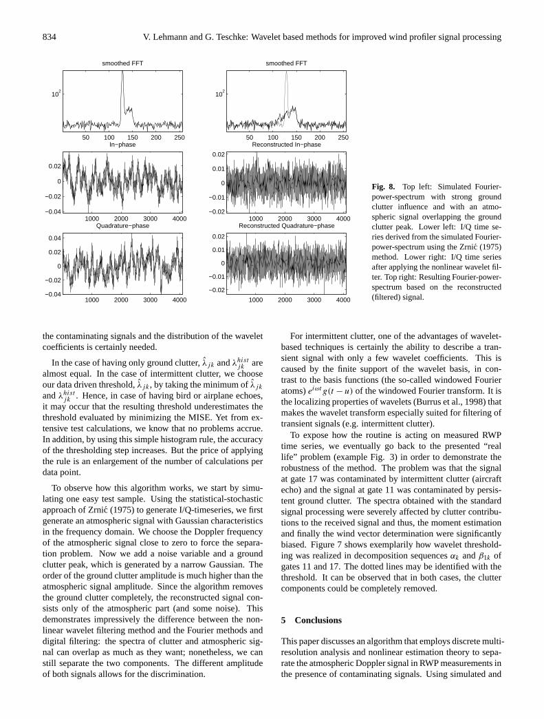
Fig. 7. Decomposition (αk und β1k),reconstruction and Fourier power spec-trum of gate 17 (top) and gate 11 (be-low). The black curves in the powerspectra representations display the de-contaminated spectra. One clearly rec-ognizes are the differences of momentestimations; see the computed first mo-ment before (gray arrow) and after(black arrow) the filtering step.

one can detect the smallest valueq0 with Hj (q0) ≤ cj,α (so-called empiricalα-quantile). If we now determine a lowerbound for the number of coefficients we want to have avail-able for reconstructing, we may easily evaluateqj,α by solv-ing∫ qj,α

−qj,α

hj (k)dk = cj,α.

We define the histogram-based threshold byλhistjk := qj,α.

Since there is only empirically information and no modelabout the characteristics of intermittent clutter echoes, we as-sume that the histogram method should remove a maximumof 15 percent of the observations and hence, we have cho-sencj,α = 0.85. This is, of course, just a heuristic value.For our dataset, this value has given the best results for theloss function. We are quite confident that the rule is robustif a larger percentage of the dwell time is contaminated withflier echos. However, more research about the properties of


50 100 150 200 250

102

smoothed FFT

1000 2000 3000 4000−0.04

−0.02

0

0.02

0.04

Quadrature−phase1000 2000 3000 4000

−0.04

−0.02

0

0.02

In−phase

1000 2000 3000 4000−0.02

−0.01

0

0.01

0.02

Reconstructed In−phase

1000 2000 3000 4000

−0.02

−0.01

0

0.01

0.02

Reconstructed Quadrature−phase

50 100 150 200 250

102

smoothed FFT

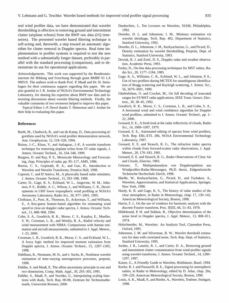
Fig. 8. Top left: Simulated Fourier-power-spectrum with strong groundclutter influence and with an atmo-spheric signal overlapping the groundclutter peak. Lower left: I/Q time se-ries derived from the simulated Fourier-power-spectrum using the Zrnic (1975)method. Lower right: I/Q time seriesafter applying the nonlinear wavelet fil-ter. Top right: Resulting Fourier-power-spectrum based on the reconstructed(filtered) signal.

the contaminating signals and the distribution of the waveletcoefficients is certainly needed.

In the case of having only ground clutter,λjk andλhistjk arealmost equal. In the case of intermittent clutter, we chooseour data driven threshold,λjk, by taking the minimum ofλjkandλhistjk . Hence, in case of having bird or airplane echoes,it may occur that the resulting threshold underestimates thethreshold evaluated by minimizing the MISE. Yet from ex-tensive test calculations, we know that no problems accrue.In addition, by using this simple histogram rule, the accuracyof the thresholding step increases. But the price of applyingthe rule is an enlargement of the number of calculations perdata point.

To observe how this algorithm works, we start by simu-lating one easy test sample. Using the statistical-stochasticapproach of Zrnic (1975) to generate I/Q-timeseries, we firstgenerate an atmospheric signal with Gaussian characteristicsin the frequency domain. We choose the Doppler frequencyof the atmospheric signal close to zero to force the separa-tion problem. Now we add a noise variable and a groundclutter peak, which is generated by a narrow Gaussian. Theorder of the ground clutter amplitude is much higher than theatmospheric signal amplitude. Since the algorithm removesthe ground clutter completely, the reconstructed signal con-sists only of the atmospheric part (and some noise). Thisdemonstrates impressively the difference between the non-linear wavelet filtering method and the Fourier methods anddigital filtering: the spectra of clutter and atmospheric sig-nal can overlap as much as they want; nonetheless, we canstill separate the two components. The different amplitudeof both signals allows for the discrimination.

For intermittent clutter, one of the advantages of wavelet-based techniques is certainly the ability to describe a tran-sient signal with only a few wavelet coefficients. This iscaused by the finite support of the wavelet basis, in con-trast to the basis functions (the so-called windowed Fourieratoms)eiωtg(t − u) of the windowed Fourier transform. It isthe localizing properties of wavelets (Burrus et al., 1998) thatmakes the wavelet transform especially suited for filtering oftransient signals (e.g. intermittent clutter).

To expose how the routine is acting on measured RWPtime series, we eventually go back to the presented “reallife” problem (example Fig. 3) in order to demonstrate therobustness of the method. The problem was that the signalat gate 17 was contaminated by intermittent clutter (aircraftecho) and the signal at gate 11 was contaminated by persis-tent ground clutter. The spectra obtained with the standardsignal processing were severely affected by clutter contribu-tions to the received signal and thus, the moment estimationand finally the wind vector determination were significantlybiased. Figure 7 shows exemplarily how wavelet threshold-ing was realized in decomposition sequencesαk andβ1k ofgates 11 and 17. The dotted lines may be identified with thethreshold. It can be observed that in both cases, the cluttercomponents could be completely removed.

5 Conclusions

This paper discusses an algorithm that employs discrete multi-resolution analysis and nonlinear estimation theory to sepa-rate the atmospheric Doppler signal in RWP measurements inthe presence of contaminating signals. Using simulated and


real wind profiler data, we have demonstrated that waveletthresholding is effective in removing ground and intermittentclutter (airplane echoes) from the RWP raw data (I/Q time-series). The presented wavelet based filtering technique isself-acting and, therewith, a step toward an automatic algo-rithm for clutter removal in Doppler spectra. Real time im-plementation in profiler systems is required to test the newmethod with a substantially longer dataset, preferably in par-allel with the standard processing (comparison), and to de-monstrate its use for operational applications.

Acknowledgements.This work was supported by the Bundesmin-isterium fur Bildung und Forschung through grant BMBF 01 LA9905/9. The authors wish to thank Prof. P. Maaß and Dr. H. Stein-hagen for their continuous support regarding this paper. We arealso grateful to J. R. Jordan of NOAA’s Environmental TechnologyLaboratory, for sharing his expertise about RWP raw data and in-teresting discussions about wavelet filtering methods. Finally, thevaluable comments of two reviewers helped to improve this paper.

Topical Editor J.-P. Duvel thanks T. Shimomai and J. Jordan fortheir help in evaluating this paper.

References

Barth, M., Chadwick, R., and van de Kamp, D., Data processing al-gorithms used by NOAA’s wind profiler demonstration network,Ann. Geophysicae, 12, 518–528, 1994.

Boisse, J.-C., Klaus, V., and Aubagnac, J.-P., A wavelet transformtechnique for removing airplane echos from ST radar signals, J.Atmos. Oceanic Technol., 16, 334–346, 1999.

Burgess, D. and Ray, P. S., Mesoscale Meteorology and Forecast-ing, chap. Principles of radar, pp. 85–117, AMS, 1986.

Burrus, C. S., Gopinath, R. A., and Guo, H., Introduction toWavelets and Wavelet Transforms, Prentice Hall, 1998.

Capsoni, C. and D’Amico, M., A physically based radar simulator,J. Atmos. Oceanic Technol., 15, 593–598, 1998.

Carter, D., Gage, K. S., Ecklund, W. L., Angevine, W. M., John-ston, P. E., Riddle, A. C., Wilson, J., and Williams, C. R., Devel-opments in UHF lower tropospheric wind profiling at NOAA’sAeronomy Laboratory, Radio Sci., 30, 977–1001, 1995.

Clothiaux, E., Penc, R., Thomson, D., Ackerman, T., and Williams,S., A first-guess feature-based algorithm for estimating windspeed in clear-air doppler radar spectra, J. Atmos. Oceanic Tech-nol., 11, 888–908, 1994.

Cohn, S. A., Goodrich, R. K., Morse, C. S., Karplus, E., Mueller,S. W., Cornman, L. B., and Weekly, R. A., Radial velocity andwind measurement with NIMA: Comparisons with human esti-mation and aircraft measurements, submitted to J. Appl. Meteor.,1–25, 2000.

Cornman, L. B., Goodrich, R. K., Morse, C. S., and Ecklund, W. L.,A fuzzy logic method for improved moment estimation fromDoppler spectra, J. Atmos. Oceanic Technol., 15, 1287–1305,1998.

Dahlhaus, R., Neumann, M. H., and v. Sachs, R., Nonlinear waveletestimation of time-varying autoregressive processes, preprint,1998.

Dahlke, S. and Maaß, P., The affine uncertainty principle in one andtwo dimensions, Comp. Math. Appl., 30, 293–305, 1995.

Dahlke, S., Maaß, P., and Teschke, G., Interpolating scaling func-tions with duals, Tech. Rep. 00-08, Zentrum fur Technomathe-matik, Universitat Bremen, 2000.

Daubechies, I., Ten Lectures on Wavelets, SIAM, Philadelphia,1992.

Donoho, D. L. and Johnstone, I. M., Minimax estimation viawavelet shrinkage, Tech. Rep. 402, Department of Statistics,Stanford University, 1992.

Donoho, D. L., Johnstone, I. M., Kerkyacharian, G., and Picard, D.,Density estimation by wavelet thresholding, Preprint, Dept. ofStatistics, Stanford University, 1993.

Doviak, R. J. and Zrnic, D. S., Doppler radar and weather observa-tion, Academic Press, 1993.

Farley, D., On-line data processing techniques for MST radars, Ra-dio Sci., 20, 1177–1184, 1985.

Gage, K. S., Williams, C. R., Ecklund, W. L., and Johnston, P. E.,Use of two profilers during MCTEX for unambiguous identifica-tion of Bragg scattering and Rayleigh scattering, J. Atmos. Sci.,56, 3679–3691, 1999.

Ghebrebrhan, O. and Crochet, M., On full decoding of truncatedranges for ST/MST radar applications, IEEE Trans. Geosci. Elec-tron., 30, 38–45, 1992.

Goodrich, R. K., Morse, C. S., Cornman, L. B., and Cohn, S. A.,A horizontal wind and wind confidence algorithm for Dopplerwind profilers, submitted to J. Atmos. Oceanic Technol., pp. 1–22, 2000.

Gossard, E. E., A fresh look at the radar reflectivity of clouds, RadioSci., 14, 1089–1097, 1979.

Gossard, E. E., Automated editing of spectra from wind profilers,Tech. Rep. ERL-ETL 286, NOAA Environmental TechnologyLaboratory, 1997.

Gossard, E. E. and Strauch, R. G., The refractive index spectrawithin clouds from forward-scatter radar observations, J. Appl.Meteor., 20, 170–183, 1981.

Gossard, E. E. and Strauch, R. G., Radar Observations of Clear Airand Clouds, Elsevier, 1983.

Griesser, T., Multipeakanalyse von Dopplerspektren ausWindprofiler-Radar-Messungen, Ph.D. thesis, EidgenossischeTechnische Hochschule Zurich, 1998.

Hardle, W., Kerkyacharian, G., Picard, D., and Tsybakov, A.,Wavelets, Approximation, and Statistical Applications, Springer,New York, 1998.

Hardy, K. R. and Gage, K. S., The history of radar studies of theclear atmosphere, in Radar in Meteorology, chap. 17, 130–142,American Meteorological Society, Boston, 1990.

Harris, F. J., On the use of windows for harmonic analysis with thediscrete Fourier transform, Proc. IEEE, 66, 51–83, 1978.

Hildebrand, P. H. and Sekhon, R., Objective determination of thenoise level in Doppler spectra, J. Appl. Meteor., 13, 808–811,1974.

Holschneider, M., Wavelets: An Analysis Tool, Clarendon Press,Oxford, 1995.

Johnstone, I. M. and Silverman, B. W., Wavelet threshold estima-tors for data with correlated noise, Tech. Rep. Dept. of Statistics,Stanford University, 1995.

Jordan, J. R., Lataitis, R. J., and Carter, D. A., Removing groundand intermittent clutter contamination from wind profiler signalsusing wavelet transforms, J. Atmos. Oceanic Technol., 14, 1280–1297, 1997.

Kaiser, G., A Friendly Guide to Wavelets, Birkhauser, Basel, 1994.Keeler, R. J. and Passarelli, R. E., Signal processing for atmospheric

radars, in Radar in Meteorology, edited by D. Atlas, chap. 20a,199–229, American Meteorological Society, Boston, 1990.

Louis, A. K., Maaß, P., and Rieder, A., Wavelets, Teubner, Stuttgart,1998.


Mallat, S., Multiresolution approximations and wavelet orthonor-mal bases ofL2(R)., Trans. Amer. Math. Soc., 69–87, 1989.

Mallat, S., A Wavelet Tour of Signal Processing, Academic Press,1999.

May, P. T. and Strauch, R. G., An examination of wind profiler sig-nal processing algorithms, J. Atmos. Oceanic Technol., 6, 731–735, 1989.

May, P. T. and Strauch, R. G., Reducing the effect of ground clut-ter on wind profiler velocity measurements, J. Atmos. OceanicTechnol., 15, 579–586, 1998.

Meyer, Y., Wavelets: Algorithms and Applications, SIAM,Philadelphia, 1993.

Monna, W. A. and Chadwick, R. B., Remote-sensing of upper-airwinds for weather forecasting: Wind-profiler radar, Bull. WMO,47, 124–132, 1998.

Morse, C. S., Goodrich, R. K., and Cornman, L. B., The NIMAmethod for improved moment estimation from Doppler spectra,submitted to J. Atmos. Oceanic Technol., 1–24, 2000.

Muschinski, A., Sullivan, P. P., Wuertz, D. B., Hill, R. J., Cohn,S. A., Lenschow, D. H., and Doviak, R. J., First synthesis ofwind-profiler signals on the basis of large-eddy simulation data,Radio Sci., 34, 1437–1459, 1999.

Papoulis, A., Probability, Random Variables and Stochastic Pro-cesses, McGraw-Hill, 3 edn., 1991.

Petitdidier, M., Sy, A., Garrouste, A., and Delcourt, J., Statisticalcharacteristics of the noise power spectral density in UHF andVHF wind profilers, Radio Sci., 32, 1229–1247, 1997.

Ralph, F. M., Neiman, P. J., van de Kamp, D. W., and Law, D. C.,Using spectral moment data from NOAA’s 404-MHz radar windprofilers to observe precipitation, Bull. Amer. Meteorol. Soc., 76,1717–1739, 1995.

Ralph, F. M., Neiman, P. L., and Ruffieux, D., Precipitation identi-fication from radar wind profiler spectral moment data: Verticalvelocity histograms, velocity variance, and signal power – ver-tical velocity correlation, J. Atmos. Oceanic Technol., 13, 545–559, 1996.

Rottger, J. and Larsen, M., UHF/VHF radar techniques for atmo-spheric research and wind profiler applications, in Radar in Me-teorology, chap. 21a, 235–281, American Meteorological Soci-ety, Boston, 1990.

Schmidt, G., Ruster, R., and Czechowsky, P., Complementary codeand digital filtering for detection of weak VHF radar signals

from the Mesosphere, IEEE Trans. Geosci. Electron., GE-17,154–161, 1979.

Schumann, R. S., Taylor, G. E., Merceret, F. J., and Wilfong, T. L.,Performance characteristics of the Kennedy Space Center 50MHz Doppler Radar wind profiler using the median filter /first-guess data reduction algorithm, J. Atmos. Oceanic Technol., 16,532–549, 1999.

Spano, E. and Ghebrebrhan, O., Pulse coding techniques forST/MST radar systems: A general approach based on a matrixformulation, IEEE Trans. Geosci. Remote Sensing, 34, 304–316,1996.

Stark, H.-G., Continuous wavelet transform and continuous multi-scale analysis, Math. Anal. and Appl., 169, 179–196, 1992.

Steinhagen, H., Dibbern, J., Engelbart, D., Gorsdorf, U., Lehmann,V., Neisser, J., and Neuschaefer, J. W., Performance of the firstEuropean 482 MHz wind profiler radar with RASS under opera-tional conditions, Meteorol. Z., N.F.7, 248–261, 1998.

Sulzer, M. and Woodman, R., Quasi-complementary codes: A newtechnique for MST radar sounding, Radio Sci., 19, 337–344,1984.

Teschke, G., Komplexwertige Wavelets und Phaseninformation,Anwendungen in der Signalverarbeitung, Diplomarbeit, Institutfur Mathematik, Universitat Potsdam, 1998.

Tsuda, T., Middle Atmosphere Program – Handbook for MAP,vol. 30, chap. Data Acquisition and Processing, pp. 151–183, ICSU Scientific Committee on Solar-Terrestrial Physics(SCOSTEP), ISAR 24–28 November 1988, Kyoto, 1989.

v. Sachs, R. and MacGibbon, B., Nonparametric curve estimationby wavelet thresholding with locally stationary errors, preprint,1998.

Vetterli, M. and Kovacevic, J., Wavelets and Subband Coding, Pren-tice Hall PTR, New Jersey, 1995.

Wilfong, T. L., Merritt, D. A., Lataitis, R. J., Weber, B. L., Wuertz,D. B., and Strauch, R. G., Optimal generation of radar wind pro-filer spectra, J. Atmos. Oceanic Technol., 16, 723–733, 1999a.

Wilfong, T. L., Merritt, D. A., Weber, B. L., and Wuertz, D. B.,Multiple signal detection and moment estimation in radar windprofiler spectral data, submitted to J. Atmos. Oceanic Technol.,1999b.

Zrnic, D. S., Simulation of weatherlike Doppler spectra and signals,J. Appl. Meteor., 14, 619–620, 1975.

Documents

Wavelet based methods for improved wind profiler signal processing