Embed Size (px)
Citation preview

!ETA - GAMMA - GAMMA CORRELATION IN Mn56 :
A TEST OF TIME REVERSAL !NV ARIANCE
by
Martin Henry Garrell !.A., Princeton University, 1960
M.s., University o~ Illinois, 1963
Ph.D. Dissertation June, 1966
!ETA..;GAMMA·GAMMA CORRELATION,IN Mn56
A TEST OF TIME REVERSAL INVARIANCE
Martin Henry Garrell, Ph.D.
Department of Physics
University of Illinois, 1966
An experiment to measure time reversal violation in two p-r-o cas-56
cades of Mn {2.58 h) is discussed. We show how one measures the inter-
ference terms in f-Y-( correlations using experimental quantities. We
explain in detail the systematic errors involved in an accurate correlation
experiment and point out the inherent limitations of such an experiment
for time reversal measurements. Particular attention is given to descrip-
tions of the electronics system used. From measurements of the interference 56
terms in two 0 transitions of Mn , we conclude that the phase difference
between Ml and E2 reduced matrix elements is { 3.3 ± 3.0 )·10-2 and { -4.3 ~ -2 4.0 )•10 for the 1.81 and 2.12 MeV transitions respectively.
ACKNOWLEDGEMENTS
The author wishes to express sincere appreciation to the following
people who aided him in this experiment:
Professor Hans Frauenfelder, who provided ideas~ impetus, and
understanding of many of the basic problems. With him, the many years
of graduate study have been often hectic, but always thoroughly
enjoyable and educational.
Professor David Sutton, without whose knowledge of electronics
and insight into experimental physics, the experiment could not have
been performed.
Mr. Daniel Ganek, whose help in setting up the electronics, pre-
paring sources, and programming data was invaluable.
The staff of the University of Illinois Reactor Laboratory,
especially Messrs. Gerald Beck, Paul Hesselman, and Sidney Boudreaux,
who put in long hours and weeks irradiating our samples.
The staff of the Physics Research Laboratory, who made available
the facilities and apparatus needed for the experiment.
Mrs. Barbara Anderson, who typed this thesis.
iti
The author also wishes to thank many others who helped him in his
academic career, including Professors Peter Debrunner, Giovanni DePasquali,
Hendrik de Waard, and Gerald Almy, Mr. Muzaffer Atac, and Drs. Rollin
Morrison and David Hafemeister.
The author wishes to express his appreciation to his wife Janet,
whose understanding and encouragement were vital to him in the sometimes
discouraging years of research and graduate study.
Finally, the author acknowledges the inspiration given to him by
the fields and streams of the Midwest.
TABLE OF CONTENTS
I. INTRODUCTION •
II.
III.
IV.
DECAY OF Mn56 • • •
A. The Cascade
!. The Reduced Matrix Element Ratios
C. Scintillation Spectra
THEORY •
A. Inspection of £ •
!. Experimental Measurement of Triple Correlations ~ C. Another Method for Determining ~ ,.
D. Statistics for Determination of E.
EQUIPMENT AND PROCEDURES •
A. Physical Layout
1. Detectors • •
2. Sources and Source Frame • •
!. Procedure
c. Electronics • •
1. Accidental Count Rates . 2. Pulse Sampling • •
3. Twofold Fast Coincidences
4. Pulse Height Analysis •
5. Trigger Gating • • •
6. Slow Coincidence Network . •
7. Isolation
iv
1
5
5
5
8
. 13
. 13
. 15
• 22
• 23
• 26
• 26
• 26
• 26
• • 27
• • 27
• • 27
• 31
• • 31
• 31
• 32
• 32
• 33
v
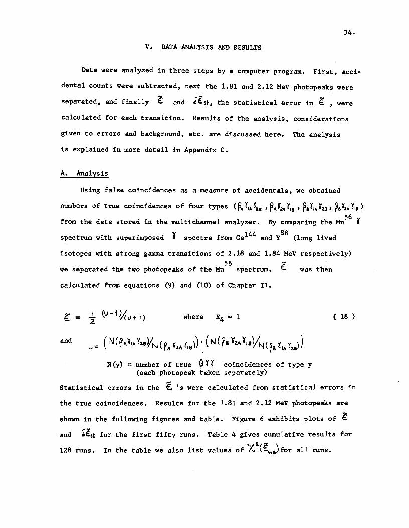
V. DATA ANALYSIS AND RESULTS • • • • • • • • • • • • • • • • • • • 34
A. Analysis . . . . . • • • 0 • • • • • • • • • • • • • • • • 34
!. :Background Effects • • . . . . . . . . . . . . . . . . . . 38
1. Compton Scattering . . . . . . . . . . . . . . . . . . 38
2. Na24 :Background • . . . . . . . . . . . . . . . . . . . 41
c. Checks for Additional Errors . . . . . . . . . . . . . . . 41
D. Normalizing by Using.·~ 4 Coincidences . - . . . . . . . . . 41
E. Conclusion . . . . . . . . . . . . . . . . . . . . . . . . 42
APPENDIX A. !ETA-GAMMA-GAMMA CORRELATION . . . . . . . . . . . . . . 45
APPENDIX !. ELECTRONICS ••••••• . . . . . . . . . . . . . . . . 51
1. Fast Coincidence Circuitry . . . . . . . . . . . . . . . . 51
2. Coincidence Efficiencies . . . . . . . . . . . . . . . . . 56
3. Miscellaneous Tests . . . . . . . . . . . . . . . . . . . . 61
APPENDIX C. DATA PROCESSING . . . . • • • • • • • . . . . . . . . . . 62
1. Correcting for Accidental Coincidences . . . . . . . . 62
2. Separation of 1.81 and 2.12 MeV Photopeaks •••••••• 73
3. ,.. &-Calculation of €. and . €.. st. from Data • • • • • ••••• 74
4. Normalization Using Coincidences • • . . . . . . . . . 74
!I!LIOGRAPHY • • • • • • . . . . . . . . . . . . . . . . . . . . . . . 76
1.
I • INTRODUCTION
In 1957, when parity (P) and charge conjugation (C) violation were
found for weak interactions, physicists began to ask whether time reversal
(T) invariance existed for every physical process. At that time and for
seven years afterwards, all experiments indicated T invariance.* Because
all present field theories are invariant with respect to the product of
C, P, and T taken in any order, T invariance implies invariance of the
combined operation CP.
Then, in 1964, Christenson, Cronin,
the two-pion-decay mode of the long-lived
Fitch, and Turlay 1/discovered 0
component K2 of the neutral K
meson. Since the two-pion-decay mode is of different CP than the predominant 0
three-pion mode, the K2 decay violates CP invariance. Because of the CPT
theorem, CP breakdown implies T violation. Many suggestions were offered
as explanations for the violation of CP and T. The hypothesis of !ern-
stein, Feinberg, and Lee~that T violation could arise in the electro-
magnetic interaction is of particular interest to us for ou~ experiment. 11 From the work of Lloyd one can show that T invariance has the follow-
ing consequence: The ratio of certain reduced matrix elements which occur
in the theory of angular correlations is real. Thus, one possible way to
test for T violation is to look at the interference term in a mixed ~
transition and to try to detect the imaginary part of the reduced matrix
element ratio. Because this interference term is small, it is difficult
to measure.
*For discussions of the symmetry principles, see J. J. Sakurai, Invariance Princi les and Elementa Particles, (Princeton University Press, Prince-ton, 1964 and T .• D. Lee, Phys. Today 12., 1!3, 23 (1966).

My thesis is based on a suggestion of Lee and Yan~ -- amplified
by Henley and Jacobsohn~ Stichel~ and DeSabbataZI-- that T invariance
2.
can be tested in nuclear interactions by means of {3- "( - 0 angular corre-
lation experiments. Fuschini, Gadjokov, Maroni, and Veronesi~ performed 47 106 experiments of this type in 1963-1964 with Ca and Rh • In the latter
"' -4 case, they claimed to have measured an interference term € = (5 ± 7) • 10
from which they found the phase angle of the reduced matrix element ratio -2
~~sin 7. = (3 ± 4) • 10 •
We have tested time reversal invariance using two triple cascades
in Mn56 (2.58 h). In each cascade a Gamow-Teller decay is followed by an
electromagnetic Ml-E2 mixed transition and then by a pure E2 transition. 56
We chose Mn for our experiment for two reasons. The two cascades have
mixing ratios that are different in sign and magnitude, and o's of interest
are easily resolved by scintillation detectors.
Our experiment differs from its predecessors in several respects.
We used an elaborate system of modular electronics in order to obtain over-
all stability, high coincidence counting efficiency, and accurate accidental
count rate corrections. We arranged our counters and interpreted our data
in such a way as to reduce systematic errors. Finally, we were able to
obtain smaller statistical errors in the measurement of the interference
term. For the two cascades observed, we found the results given in Table 1.
The second chapter of this thesis is devoted to a brief discussion 56 of the decay of Mn • The following chapter deals with the triple corre-
lation equation and its application to our experiment. The physical con-
figurations of the experiment (sources, counters, etc.), the conditions for
running the experiment, and the essentials of the electronics circuitry
are described in Chapter IV. The final chapter presents the data that
3.
Table 1 ,...,
Experimental Results for E:., ( &rz.>, and ~
Er 1.81 MeV 2.12 MeV
& 0.18 -0.28
"' (3 .1±. 2 .9)• 10-4 E: (6.5±6.0)•10 -4
(6rz.) + -3 (5.9- !).5)•10 (12 .2 ± 11.2) •10-3
~ (3.3± 3.0)·10-2 + -2 (-4.3-4.0)•10
4.
were accumulated and an interpretation of these data.
Three appendices follow.
method for analyzing the
7/ The first is a summary of DeSabbata's-56 correlation as it applies to the Mn
cascades, the second is a detailed discussion of the electronics, and the
last presents an example of data analysis for a typical run.
5.
II. DECAY OF Mn56
A. The Cascade
The decay of Mn56 , as illustrated in Figure 1, has two branches that + + + .... follow the 3 -2- 2 --o spin sequence. I shall refer to these branches
in all that follows as the 1.81 MeV or 24% branch and the 2.12 MeV or 15%
branch, according to the ~nergies of the first (mixed)gammas of the cas-
cades or according to the branching ratios.
B. The Reduced Matrix Element Ratios
The reduced matrix element ratio for a mixed gamma transition enters
into the ~¥o correlation equations, as shown in Appendix A. Its role in
the determination of the time reversal violation is discussed in the follow-
ing chapter. Several authors have measured the reduced matrix element
ratios for both mixed gammas. 9•10 •11/ Averaging their experimental values,
one obtains = +0.18±"0.03 for the 1.81 MeV transition and -0.28±0.03
for the 2.12 MeV transition. As a check on our coincidence circuitry, we
also measured these reduced matrix element ratios by means of standard
correlation techniques. We found values of 0.13±0.03 and -0.24±0.02, in
reasonable agreement with the above.
Having two cascades of about equal energy but with different d's
is advantageous for our experiment. By a suitable choice of energy dis-
criminator levels, we can observe triple correlations for both cascades in
the same experiment. We expect to get two independent determinations of
time reversal violation in this manner.

6.
Figure 1. Decay scheme of Mn56 • Only predominant branches are shown.
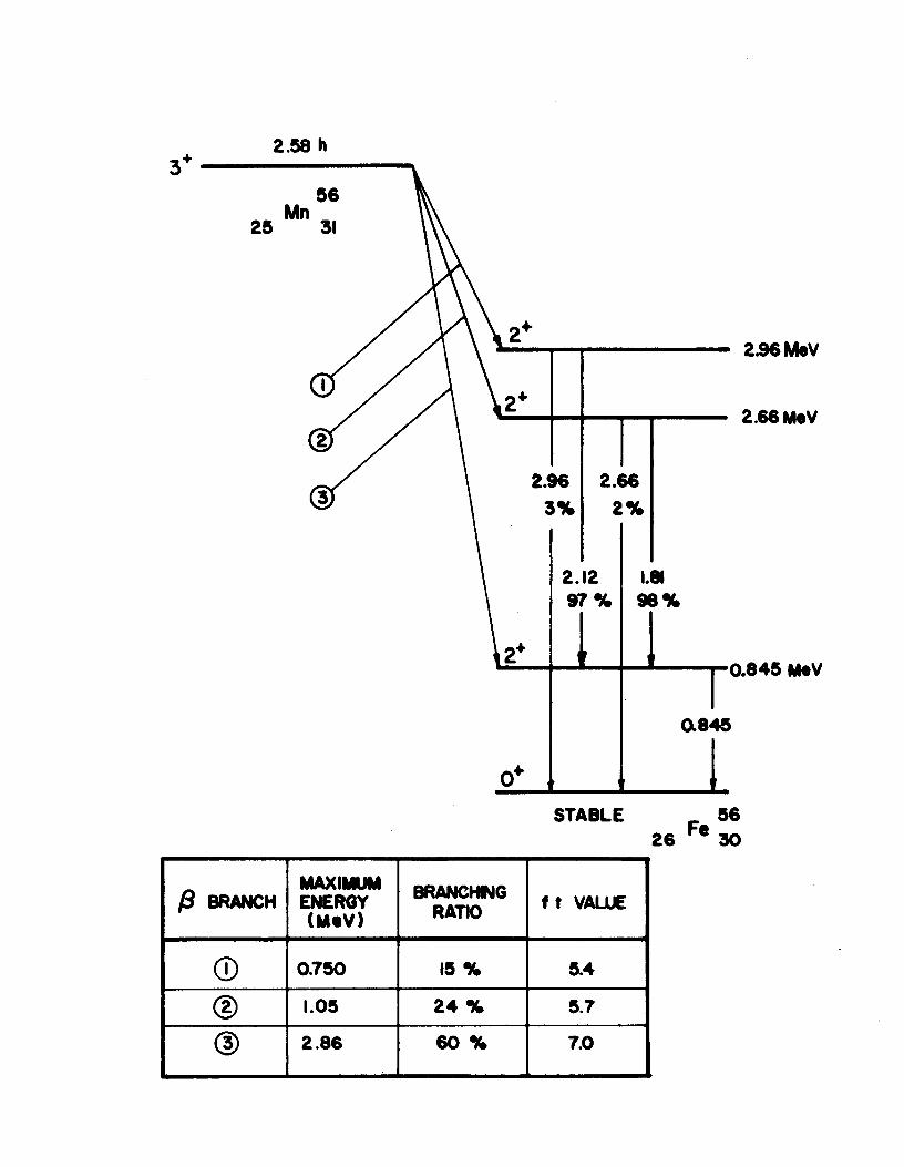
2.58 h 3·--------------~
56 Mn
25 31
~ BRANCH MAXIMUM ENERGY (MeV)
CD 0.750
® I.O!S
@ 2.86
BRANCHWG RATIO
15%
24%
60%
2.66MeV
2.96 2.66 3% 2%
2.12 1.81 97% 98%
0.845
STABLE F 56 26 • 30
f t VAl..LE
5.4
5.7
7.0

8.
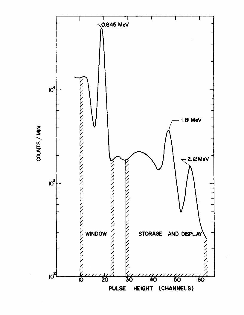
C. Scintillation Spectra
The typical gamma and beta spectra of Mn56 which are shown in
Figures 2a and 2b were obtained with our scintillation detectors (described
in Chapter IV). The shaded portions of the spectra show the energies of
interest for the coincidence experiment.
9.
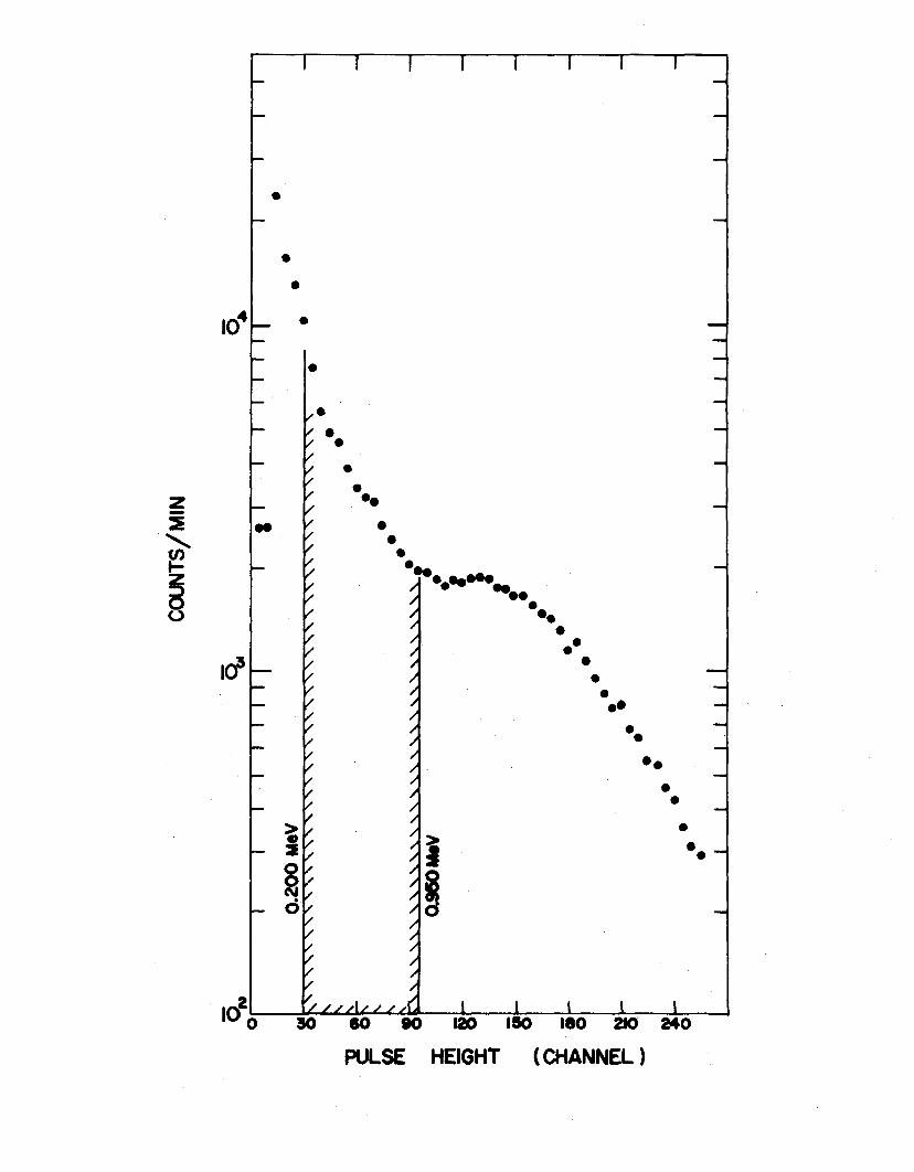
Figure 2a. 56 Typical gamma spectrum of Mn source. The shaded
portions are regions used for the coincidence experiment,
The lower shaded portion is the 0.845 MeV window, and
the upper shaded portion is used for display and storage
in the multichannel analyzer.
~ r l
:4 10 ·-·
"'-0.845 MeV
/ 1.81MeV
~.12MeV
STORAGE AND DISPLAY
PULSE HEIGHT (CHANNELS)
11.
56 Figure 2b. Typical beta spectrum of Mn Shaded portion is used
for (3 r 1 coincidences.
•
• •
1cr
• • • •
• •• • • • ... ......... .. •• • • •• • • • ••
•• ••
• • • ••
PULSE HEIGHT (CHANNEL )
13.
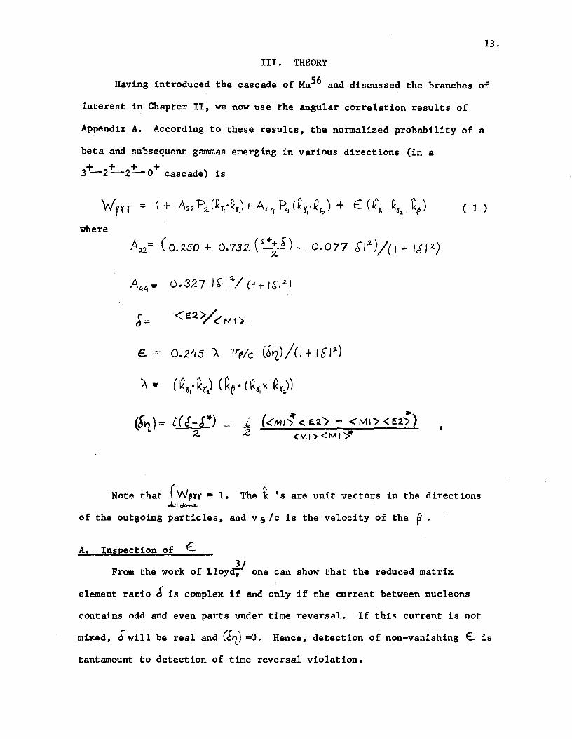
III. THEORY
Having introduced the cascade of Mn56 and discussed the branches of
interest in Chapter II, we now use the angular correlation results of
Appendix A. According to these results, the normalized probability of a
beta and subsequent gammas emerging in various directions (in a + + + + 3 -2 -2-0 cascade) is
where
= i_ (<Mt{ < E.2.) - <MI"> <E.2.~) Z <MI'> <MI >>It
( 1 )
•
Note that Jl~!:r = 1. The k 's are unit vectors in the directions
of the outgoing particles, and v f> I c is the velocity of the ~ •
A. Inspection of f:
From the work of Lloy~ one can show that the reduced matrix
element ratio J is complex if and only if the current between nucleons
contains odd and even parts under time reversal. If this current is not
mixed, ~will be real and (J'?.) =0. Hence, detection of non-vanishing E. is
tantamount to detection of time reversal violation.
14.
We can now interpret {J"()in terms of real and imaginary parts of
E (~-
tf we let (Ml> aM+ im and <E2) •E + ie,
~) • ( 2 )
complex reduced matrix elements.
where M :»m and E ~e, then
M M
This is seen to be cons is tent with (!rz) = ~ ( & - S .t) if we take
a= E+ ie. M+tm
E. ( • ( .!.. - 1'\"\ )) ~ M 1+ L E M •
(~?_) can be written
where
l~l'l) ': - JM ( ~) :! d" ( '(,Mt- 7.M~)
j = E:./M
~~ = 'M/"1
~a= e./E
( 3 )
( 4 )
Because the quantity l corresponds in first order to the experimental
reduced matrix element ratio which has been accurately determined for both
1.81 MeV and 2.12 MeV transitions from ~o correlations, and because A and
v ~ I c can also be calculated for our experiment, we can therefore measure
the phase difference ? :. (~M,-1£1) • ~- f If the hypothesis of :Bernstein,
Feinberg and Lee Y is correct, we should expect the ratios e/E and m/M
to be CJ(~~) , since these quantities are proportional to the ratios
* of even currents to odd currents.
*tn accord with a recent paper by Henley and Jacobsohn,l1/ we have assumed in all the above discussion that, although a breakdown of the :Born approx-imation may also be responsible for nonvanishing (~~),the effect of this breakdown will be several orders of magnitude smaller than the effect of time reversal-violating nuclear currents.
15.
!. Experimental Measurement of Triple Correlations.
In an experiment in which we are counting true triple coincidences
using three arbitrary counters and two two-fold coincidence circuits,
the number of true triple coincidences per second is
where
( 5 )
N0 a number of disintegrations per second.
Pt D probability Of emiSSiOn Of particle lo
P1-a = probability for emission of particle 2 if particle 1 has been
emitted.
P1a.-3 a probability for emission of particle 3 if particles 1 and 2
have been emitted. th relative width of energy selection fori particle •.
th th efficiency of i counter for detecting i particle. th solid angle subtended by i detector at the source.
E1 l2. = coincidence efficiency of the first two-fold circuit that
fires on each coincidence between particles 1 and 2.
~~3 = coincidence efficiency of the second two-fold circuit that
fires whenever the output of the first circuit is in coin-
cidence with a pulse due to particle 3.
W 1~3 a probability for detecting triple coincidences as a function
Of particle directions t defined SUCh that: ( wi"J.3 D 1. o.il cli......C.
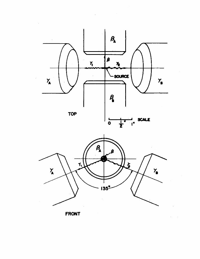
In the arrangement that we used (detectors are shown in Figure 3)
four possible types of triple coincidences can be detected. These possi-
bilities are illustrated in Figure 4.
16.
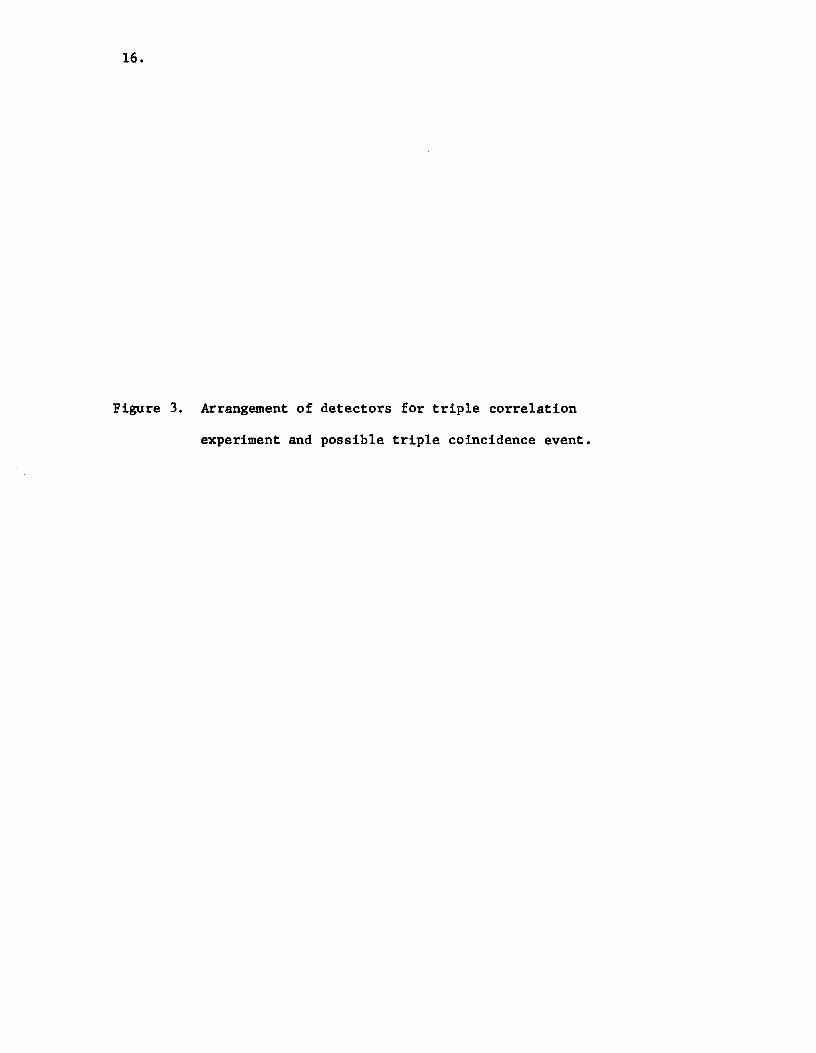
Figure 3. Arrangement of detectors for triple correlation
experiment and possible triple coincidence event.
TOP
FRONT
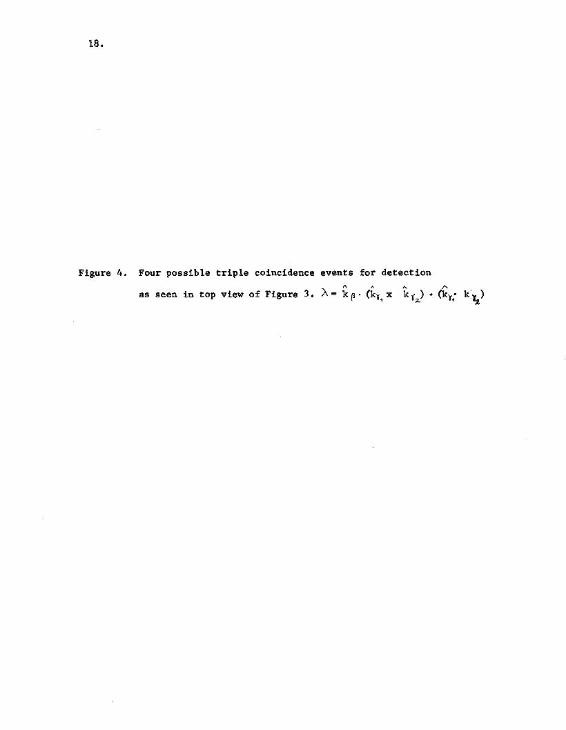
18.
Figure 4. Four possible triple coincidence events for detection 1\ " " I' as seen in top view of Figure 3. ~ = k (3 • (k\', x k '62.) • (kyt k l.2.)
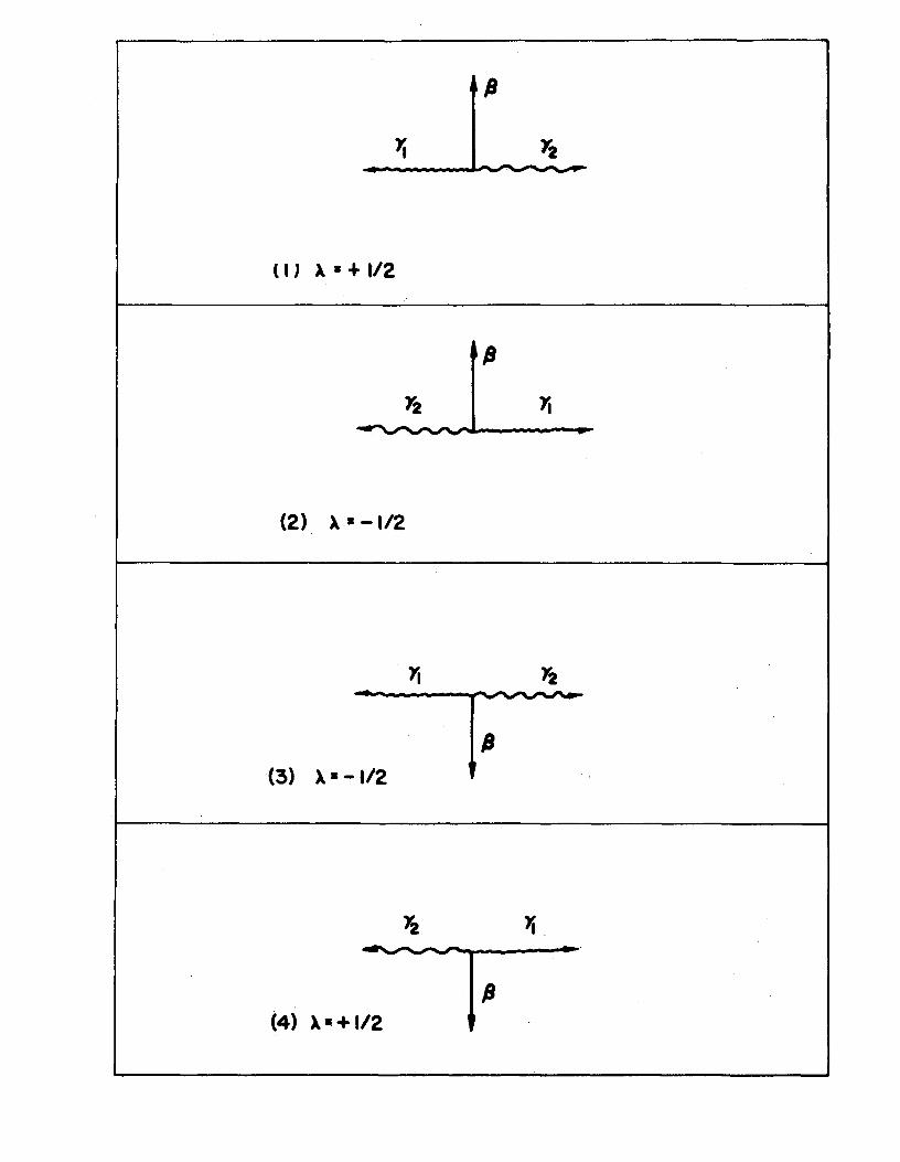
fJ
'i 1'2 ~- -·- -
(IJ A • + t/2
fJ
1'2 Yi -"'-""'"-
(2) ~. -1/2
Yi y2 - ----------fJ
(3) ~. -1/2
)i )i ~----
fJ (4) ~·+ 1/2

' 20.
TYPE 1 nflA-r,Ar:aa = No P@ "P!i-l, PPt.-ta F~A E.p,. n~A. Fr,A Er,~, JlrA F'"r2., ~8 .n.re'>< ( 6 )
I( E. ~.,..r2.e C(t,A ra.a> flA w+
TYPE 2 n~A 'fv.'(IIJ = Nof¥ ]1-r, P.r,-r .. F PA c~A n~A F O'u. E.rv. Q.A f)-,6 E.r,, nrs" I( ey2.A'~II Etr\A~II)~A w-
TYPE 3 n fie r,,. 'faa. No 'P~ P~-t,'!lr.-r .. F,IS 'C-~8 n.~e 'F¥,,. E.y,,. .nr,. Fr:Le er, • ..n 'I'&)(
~ E.'t 1,.~:a.e E<r 111 r~a)Pe W-
TYPE 4 n ,.,. YzA ~.... No'?~ 'P~-r. 'P~Y.-ra. Fl. c. @a ~8 FtlA E.y.lAnrA F(,, E.r,, .C'lr, )( ~ e.r,e.r ..... E.(tll~ll'u,)@a w+
. + -W is the function ( 1 ), and we define W and W according to the sign
of A . Then, in the experfmental situation
( 7 )
where • ( 8 )
1)1 • 1/2 for particles directed along the axes of Figure 3.
Q1, Q22 , and Q44 are the geometrical attenuation coefficients due to the
solid angles subtended by the counters at the source. If we measure the
numbers of true coincidences of all four types during the same period of
time and combine these numbers in the ratio
(TYPE 1/TYPE 2) • (TYPE 4/TYPE 3)
· ( n P! r,& r,,. / n ) far,,. r.aa
21.
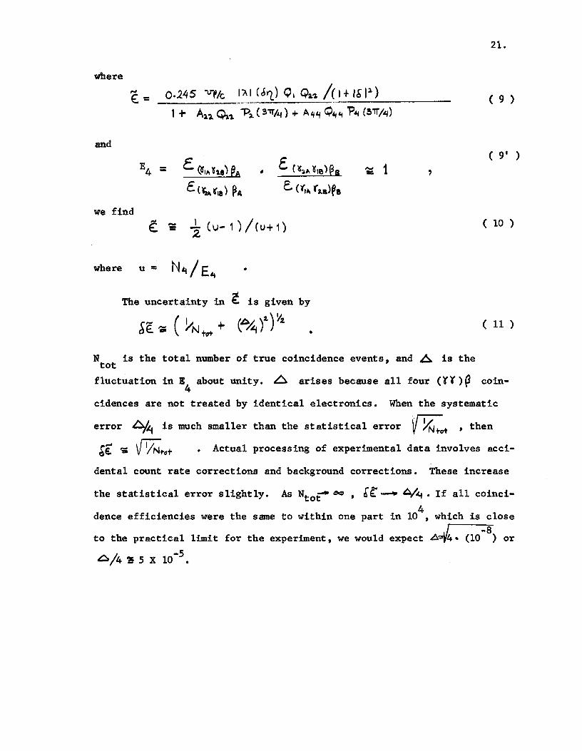
where €= o.245 v~/c I'AI(Jyt)O,Q:a.~/(1+1&1~) ( 9 )
1 + A2.'1 Q,'2. -p,_ ( 3"\TfLf) +- Aijl.j Q'l'i 'Pot; (~'TT'/"1)
and
E4 = E (ls,~ he) @A • E. C~,~. ~,e)@a ,..., 1 = ( 9' )
' E ( r_ t,a) PA e (f,~ fn)~a
we find e: :: 1<u-1)/<u+1) ( 10 )
where u = N'l / E't • ..!
The uncertainty in E: is given by
( I I.Ah, )a.. ) Y:t $€. ; liN to+ + \. ., ( 11 )
N is the total number of true coincidence events, and A is the tot fluctuation in E
4 about unity. 6 arises because all four ('r'r )~ coin-
cidences are not treated by identical electronics. When the systematic
error ~4 is much smaller than the statistical error V ~~+ , then
~~ -;; V 1/Ntct Actual processing of experimental data involves acci-
dental count rate corrections and background corrections. These increase
the statistical error slightly. As Ntot ec , [t--"" ~/41. If all coinci-
dence efficiencies were the same to within one part
to the practical limit for the experiment, we would
~/4 ~ s x 10-5 •
4 in 10 , which is close
expect ~~4• (10-S) or
22.
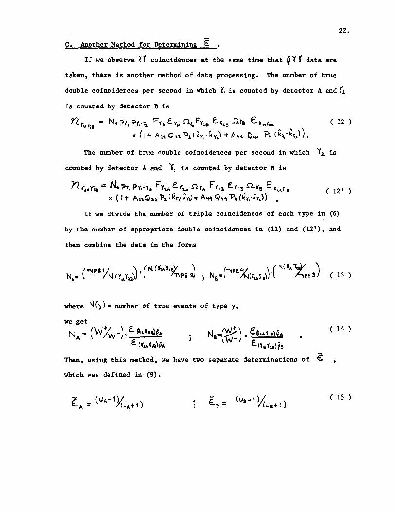
c. Another Method for Determining E . If we observe fr coincidences at the same time that ~ 't r data are
taken, there is another method of data prQcessing. The number of true
double coincidences per second in which~~ is counted by detector A and(~
is counted by detector B is
n ~A 1'2. .. No ?d I Pr,·ra. FtiA E. r,,. n·~ Fr2.5 e..l2.B n~, . e. r,,r.aa ~t (I+ AuGh~ l>a,(Qr,·ty~.) + A"'tt Q,.."1 "P4t (kr,·k.)).
( 12 )
The number of true double coincidences per second in which ~~ is
counted by detector A and 11 is counted by detector B is
Yl.r~AV"ia= No-pt,?'t,·Ya. Fy'lAE.r~.nr" ~=="r,a E.r~~~nrs E'~':~.Ar•s x ( 1 t AnOn 1>1 ( ~r,·k.-,) + A'f'l C¥ .. .~t "P~~ (kr,·ICr,)) •
( 12' )
If we divide the number of triple coincidences of each type in (6)
by the number of appropriate double coincidences in (12) and (12'), and
then combine the data in the forms
where N(~) = number of true events of type y,
we get NA .. (W;;w-). E. Cti,.ISi!i)fA
£ ( .. ,a,.(,a)PA
( 14 ) •
Then, using this method, we have two separate determinations of € which was defined in (9).
• ( 15 ) )
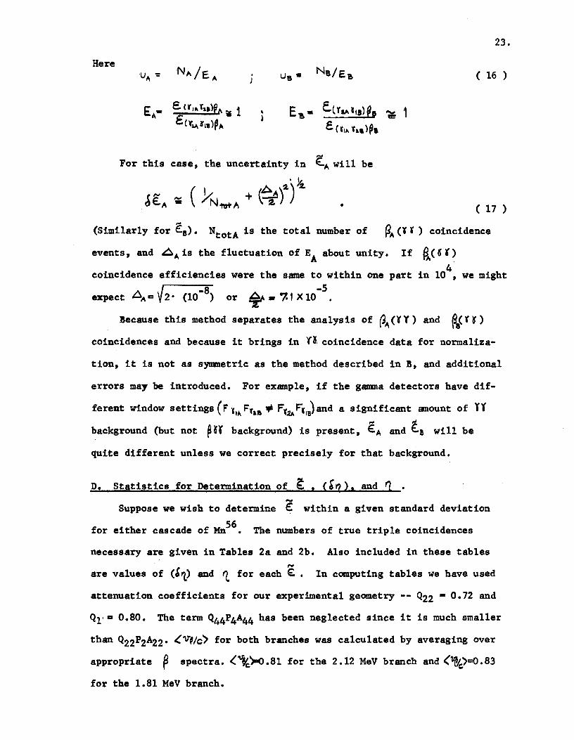
Here N~/E.A Ne/E& u" -: . \Je = )
E:A• E. U ,,.. fu)fr- 1! 1 E'&= E.t raA .,,) ~' E C'tu,l,, )P~ e. c ,,,.. t ... ),.
-For this ease, the uncertainty in E:.,.. will be
~ 2.·)~ ~e: ... ~ ( YN~tA + (~) •
23.
( 16 )
-1 e
( 17 )
(Similarly for €8). NtotA is the total number of ~~~ (¥ J' ) coincidence
events, and .6" is the fluctuation of EA about unity. If g_c ~ t) coincidence efficiencies were the same to within one part in 104, we might
~ " -8 -5 expect "• V 2 • (10 ) or ~ • '7- 1 X 10 •
Because this method separates the analysis of ~~ (l Y) and @a< t ~)
coincidences and because it brings in Y~ coincidence data for normaliza-
tion, it is not as symmetric as the method described in B, and additional
errors may be introduced. For example, if the gamma detectors have dif-
ferent window settings (F t,~ Ft,a.,;. F'r2AFr,8)and a significant amount of Y'( .... ..!.
background (but not @ rr background) is present, €." and €.a will be
quite different unless we correct precisely for that background.
D. Statistics for Determination of ~ 1 ( b 2) 1 and f1. •
Suppose we wish to determine ~ within a given standard deviation
for either cascade of Mn56 • The numbers of true triple coincidences
necessary are given in Tables 2a and 2b. Also included in these tables ,..
are values of (S rt,) and tt for each E:. • In computing tables we have used
attenuation coefficients for our experimental geometry Q22 • 0. 72 and
Q1·• 0.80. The term Q44P4A44 has been neglected since it is much smaller
than Q22P2A22• ~V,/c) for both branches was calculated by averaging over
appropriate ~ spectra. ~~).o.81 for the 2.12 MeV branch and ('k)a0.83
for the 1.81 MeV branch.

24.
Table 2a -E. , (&~) , ~ , and Stati$tics Needed for 24% !ranch (1.81 MeV)
Statistics (6rl)= 19.1 X €, ~ to Measure Std. 5.55 X Cd'l) ~ 7=
Deviation of t l
10-2 104 -2 19.1 X 10 1.06
5 X 10·3 4 X 10 4 9~55 X 10-2 5.30 X 10⁻¹
-3 6 -3 1.06 X 10⁻¹ 10 10 19.1 X 10
5 X 10•4 4 X 10⁶ 9.55 X 10⁻³ 5.30 X 10·2
10-4 8 -3 1.06 X 10⁻² 10 1.91 X 10
10-5 10 10
1.91 X 10 -4 1.06 X 10 -j

25.
Table 2b
~, a'l.), ~,and Statistics Needed for 15% !ranch (2.12 MeV)
.-4 Statistics (~'()= 18.7 X €_ e: to Measure Std. 't = -3.57 x a7.l
Deviation of :!: f.
10-2 4 -2 -1 10 18.7X10 -6.67 X 10
5 X 10•3 4 X 10⁴ -2 -1 9.35 X 10 -3.34 X 10
10-3 106 1.87 X 10⁻² -6.67 X 10 -2
5 X 10 -4
4 X 10⁶ 9.35 X 10⁻³ •3.34 X 10 -2
lo-4 108 1.87 X 10⁻³ -6.67 X 10 -3
. -5 1010 -4 -6.67 X 10⁻⁴ 10 1.87 X 10

26.
IV. EQUIPMENT AND PROCEDURES
In this chapter, we first describe the physical layout used for the
expertment including detectors, sources, and source holders. The pro-
cedure is also discussed, and typical counting data are given. For coin-
cidence measurements, we used a system of modular logic circuits. The
essential aspects of the circuits are mentioned here, and a more detailed
description follows in Appendix B.
A. Physical Layout
1. Detectors. The arrangement of our scintillation counters was
shown in the last chapter (Figure 3). The gamma detectors were Harshaw
2" X 3" Nai(Tl) Xtals with 1/4" (45 °) bevelled faces mounted on high
quantum efficiency RCA 8575 photomultiplier tubes. To eliminate betas
incident on these Xtals, 1/4" thick beryllium discs were mounted in front
of them. The beta detectors were 1-3/4" X 1/4" discs of Pilot A plastic
with 1/8" (45 ° ) bevelled faces mounted on Philips 56AVP photomultiplier
tubes. The plastic detectors were covered with two layers of quarter mil
aluminum foil to exclude all light and were mounted on the phototubes
by means of 1-3/4" X 1" lucite light pipes· and Epox-E Pilot Bond. Each
beta detector subtended a fractional solid angle of 0.200±0.008, and
each gamma detector subtended a fractional solid angle of 0.073i 0.001 at
the center of the source.
2. Sources and Source Frame. The sources were metallic layers of
manganese evaporated onto both sides of quarter mil mylar. Aluminum 2 layers, approximately 0.006 mg/cm served as bases for the manganese
deposits. Several sources were prepared with manganese layers ranging 2 from 0.05 to 0.12 mg/cm • Multiple scattering in the sources was negli-
gible; the mean scattering angle of the lowest energy betas used in the
0 coincidence experiment was less than 12 •
27.
'the entire apparatus was mounted in an aluminum frame made of 1/16"
and 1/32" sheet metal. The sources fitted into slotted lucite holders
which slipped into the frame, and the counters were rigidly fixed to vee-
shaped ways on the frame.
B. Procedure
Sources were inserted in the University of Illinois Triga Mark II
d d fl f 1.8 X 10¹² I 2 reactor an expose to a ux P about neutrons em , sec for
periods ranging from twenty minutes to one hour. Within one hour after
irradiation, the sources were placed in position, and coincidence data
were taken for periods of three to eight hours. Typical counting data
appear in Table 3. Originally, we i~tended to use more active sources,
but we found that increased activity caused severe gain shifts and anode
fatigue in the RCA 857S's.
c. Electronics
The basic block diagram of the electronics appears in Figure 5;
to avoid confusion we show only one of the two ~(rt) coincidence cir-
cuits and only four of the six routing inputs to the multichannel analyzer.
Details are explained in Appendix B. The main features are the following:
1. Accidental Count Rates. Accidental count rates were measured
throughout the experiment. Rather than using separate coincidence cir-
cuitry for this purpose, we employed the same coincidence circuits that
formed the true coincidences; this was done by using doubled pulses for
certain events. Figures are included and details are explained in
Appendix B.
Table 3
Typical Counting Data
Source #3 Irradiation Time: 30 min. Run began 37 min. after irradiation Time of run: 255 min.
Counts/sec Type of Event at !eginning
a. singles 105 1.57 X window
(38 singles window
1.65 X 10⁵
~B singles 3.97 X 10⁴ above 0. 5 MeV
~A singles 4.47 X 10⁴ above 0. 5 MeV
0 r coinc. 5.56 X 10² (true + ace.)
PA a r ) co inc • 6.95 X 10 (true +ace.)
Total Counts During Run
9 1.29 X 10
1.37 X 10⁹
3.36 X 10⁸
3.72 X 10⁸
4.56 X 10⁶
5. 70 X 105
28.
Counts/sec at End of Run
4.32 X 10⁴
4.56 X 10⁴
1.15 X 10⁴
1.26 X 10⁴
1.53 X 10²
1. 92 X 10
29.
Figure 5. Block diagram of logic circuitry and data storage.

>A AN. D't'.l2
ANODE-DYNODE 12 (ANDY A)
CQNC.
1.r
SLOW COINC.
NETWORK
Yaa ~A ___ -t ROUTE 8
TO ADC COINC. INPUTI
ANODI-DYNODI II CAMW I)
ENERGY DISCAM.·
8
1.('
COINC.
(~ JB.t Pa FAIT COINC.
@ 1024 CHANNEL
PHA (STORAGE)
AN TO
F Dl ITAL RTERS
(ltfiUT) (AD C)
F F M COINC.
ROUTING CKT.
I 4 7 I
M INPUT)
M COIN C.
2. Pulse Sampling. We sampled three pulses from each ~ photo-
multiplier tube for use in both fast and slow coincidence circuits.
Eighth dynode pulses from RCA 8575's were amplified by Stirrup double
delay line amplifiers and passed into linear gates. Pulses were taken
from the anodes and twelfth dynodes of the RCA 8575's, and coincidences
were formed by the circuits denoted "AnDy". Fast rising anode pulses
provided the timing, while dynode pulses set lower energy cutoffs of
about 0.5 MeV for these AnDy circuits. AnDy pulses formed ~o. fast
coincidences which opened the linear gates for fifty nsec at the peaks
of the amplified eighth dynode pulses.
31.
3. Twofold Fast Coincidences. Twofold coincidences were used
throughout the network. AnDy•AnDy or ~( fast coincidences mentioned in
the preceding paragraph formed ~( ~ '( ) fast coincidences with ~ pulses
from energy discriminators.
In Chapter III I pointed out the importance of having nearly-identical
coincidence efficiencies (for .the circuits that produce ~(! r ) coinci-
dences). We took delay curves and checked coincidence efficiencies
several times during the data taking, and estimate that E4 was within
2 X 10⁻⁴ of unity. From the delay curves, we estimate the resolving
times to be 12 nsec and 17 nsec for the n· and @ ( ~ r ) fast coincidence
circuits, respectively. Our method of measuring coincidence efficiencies
is discussed in Appendix !.
4. Pulse Height Analxsis. We used a Nuclear Data 1024 channel
pulse height analyzer for storage and display of coincidence information.
We stored and displayed pulse height spectra of 1.81 MeV and 2.12 MeV
coincidence ~'s. To obtain a maximum amount of information, we stored
some of the Compton spectra as well as the photopeaks, as Figure 2a. shows.
32.
To eliminate dead time and pile-up problems, the analyzer was fed signals
from the linear gates CThese signals w~re stretched and amplified to suit
the multichannel analyzer.) whenever the gates were opened by lY coinci-
dences. The energy discriminators and slow ~oincidence network differ-
entiated between 0/A r2! and OlA '(1& coincidences. :Both analog-to-
digital converters of the analy~er were operated in coincidence modes with
coincidence inputs provided by gate generators fed from the slow coinci-
dence network. A selective storage or "routing" circuit in the analyzer
sorted out different kinds of coincidences into sixteen groups of
sixty-four channels. R~ting input signals came from the slow coincidence
circuits.
5. Trigger Gating. We used four gate generators to shut off many
of the triggers in the system (i.e., triggers in the AnDy circuit, in the
~ discriminators, and in the 'If energy discriminators) for several )"sec
whenever coincidence information was stored in the multichannel analyzer.
This was done in order to avoid ambiguous routing.
6. Slow Coincidence Network. Slow coincidences were formed between
100 nsec and 50 nsec pulses produced by trigger circuits in the energy
discriminators. :Because the triggers in the energy discriminators were
gated off after each coincidence pulse and because these triggers fired
~nly when the linear gates were opened by coincidences, there were no
accidental coincidences in the slow network.

33.
7. Isolation. Four separate s~pplies provided power for the modular
equipment. The triggers, AnDy circuits, etc. associated with each
counter were powered by two different supplies, a third supply powered
the ~r coincidence modules, and a fourth supply was used for the trig-
gers and modules associated with ~(Yl) coincidences. In this manner
we avoided interaction between l circuits and prevented the ~r coin-
cidence circuits from knowing about ~ counting. The double delay line
amplifiers were powered by a common supply, however.
34.
V. DATA ANALYSIS AND RESULTS
Data were analyzed in three steps by a computer program. First, acci-
dental counts were subtracted, next the 1.81 and 2.12 MeV photopeaks were
separated, and finally ~ and cf[st, the statistical error in €. , were
calculated for each transition. Results of the analysis, considerations
given to errors and background, etc. are discussed here. The analysis
is explained in more detail in Appendix C.
A. Analysis
Using false coincidences as a measure of accidentals, we obtained
numbers Of true Coincidences of four types (~A ~lA ras t ~~ '(.2A ~IB t ~~riA ~2.5 t @e 'r.2A ~18) 56 from the data stored in the multichannel analyzer. !y comparing the Mn o
spectrum with superimposed 0 spectra from Ce144 and v88 (long lived
isotopes with strong g~a transitions of 2.18 and 1.84 MeV respectively) 56 ~
we separated the two photopeaks of the Mn spectrum. € was then
calculated from equations (9) and (10) of Chapter II.
~ = ~ (u- 1 Vc u + I ) where
and lJ = ( N( PA ~~ ... ~:l..vN( PA ¥ 2.A ~liS))·( N ( Ps Yu 'l',,yN (~a~ lA l1!))
N (y) = number of true ~ ¥ J coincidences of type y (each photopeak taken separately)
,..
( 18 )
Statistical errors in the £ 's were calculated from statistical errors in
the true coincidences. Results for the 1.81 and 2.12 MeV photopeaks are
shown in the following figures and table. Figure 6 exhibits plots of ~
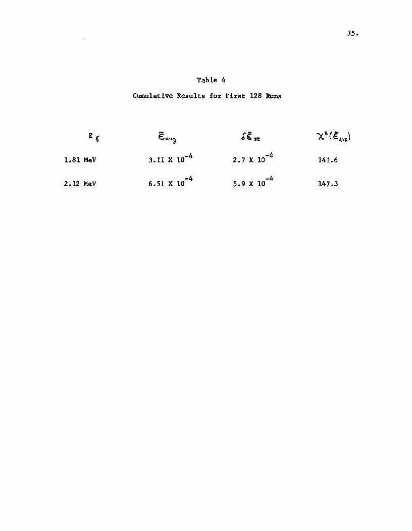
and ~~ for the first fifty runs. Table 4 gives cumulative results for
128 runs. In the table we also list values of X 1 ( ~~~vo) for all runs.
1.81 MeV
2.12 MeV
Table 4
Cumulative Results for First 128 Runs
E:Q.v~
3.11 X 10•4
6.51 X 10⁻⁴
!~rt
2. 7 X 10⁻⁴
-4 5.9 X 10
35.
147.3

36.
Figure 6. Results of first fifty runs. r-J
a. E: versus run number for 1.81 MeV photopeak.
b. ~ versus run number for 2.12 MeV photopeak.
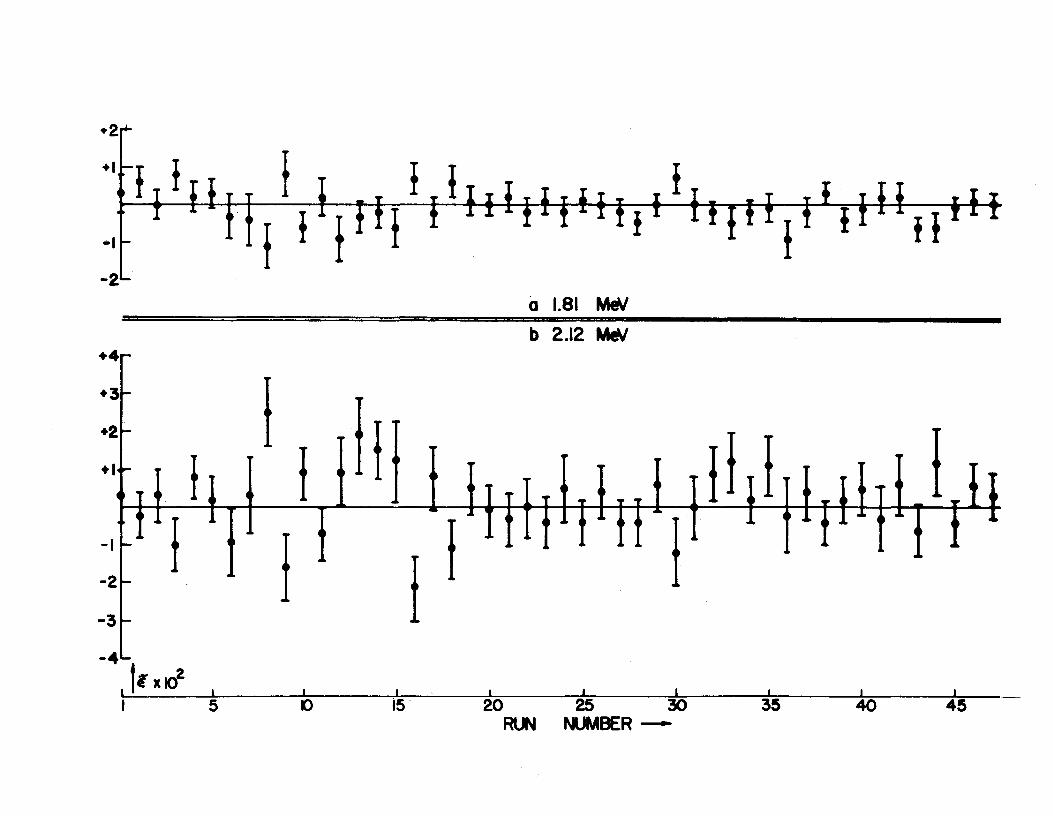
+ll-f t I T I 1 ,. ...
-1r - 1 f ~- f a 1.a1 MfN b 2.12 MfN
+4 r-
+I
~ I . . . . . . II. I . . .. L .
+3
+2
:· I 1 I ...... I .... · .... .. . .. •
I ~
-I
-2
-3
,_
-4 j,-.Kf -~---~--w:-~-~ ;;-=~----!5--w--~ 5 0 15 20 25 30 35 ~ NUMBER-
40 45
38.
( 19 )
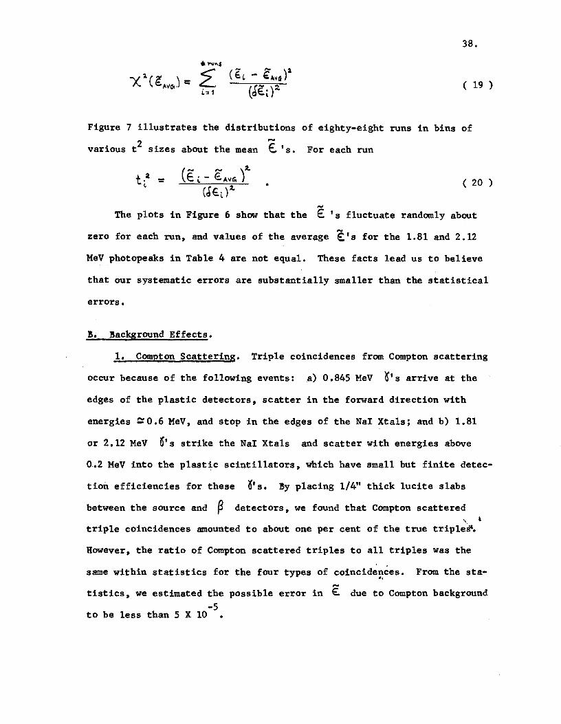
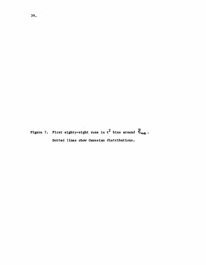
Figure 7 illustrates the distributions of eighty-eight runs in bins of
various t 2 sizes about the mean '€. 's. For each run
• ( 20 )
,... The plots in Figure 6 show that the E 's fluctuate randomly about
,... zero for each run, and values of the average €'s for the 1.81 and 2.12
MeV photopeaks in Table 4 are not equal. These facts lead us to believe
that our systematic errors are substantially smaller than the statistical
errors.
B. Bac!&round Effects.
1. Compton Scattering. Triple coincidences from Compton scattering
occur because of the following events: a) 0.845 MeV ~'s arrive at the
edges of the plastic detectors, scatter in the forward direction with
energies ~0.6 MeV, and stop in the edges of the Nai Xtals; and b) 1.81
or 2.12 MeV 6•s strike the Nai Xtals and scatter with energies above
0.2 MeV into the plastic scintillators, which have small but finite detec-
tion efficiencies for these 6• s. By placing 1/4" thick lucite slabs
between the source and ~ detectors, we found that Compton scattered '- ' triple coincidences amounted to about one per cent of the true triple~.
However, the ratio of Compton scattered triples to all triples was the
same within statistics for the four types of coincidences. From the sta-•· ,.... tistics, we estimated the possible error in ~ due to Compton background
-5 to be less than 5 X 10
39.
Figure 7. 2 ,...
First eighty-eight runs in t bins around E:A'IQ .•
Dotted lines show Gaussian distributions.
20r 20
--, 18 ~---- ~-- ~--,
I I
16 ~ -., 14 114 z I ::) I c 12 I 12
I ~ ~ I 0 010 I 10
i 8~ ---h c .., 8 I
~ 6 i 6 z I
r I L L--,
I I I
~ I I
:r '--l--i_ __ , 4
2
1 __ -·
~--r--
~--
0 0 I 0.27~ I 1.64 I 3.84 I GD
0.708 0.064 0.708 2.71 5.46 t2 __ _ t2 __ _
LSI MeV 2.12 MeV
41.
2. 24 Na Background. 24
Small amounts of Na (15 h) which may contri-
bute to coincidence spectra build up in two ways during the irradiations. 24 First, the aluminum backing on the manganese sources yields Na via (n,o<).
Secondly, improper handling may leave salt from the skin on the samples,
which produces Na24 through neutron absorption. Irradiation of a test
strip of one half mil aluminum foil showed that such background contributes
negligibly to ~l~ coincidences, and that it only contributes by about
0.1% to Yt coincidences when the samples are irradiated repeatedly.
c. Checks for Additional Errors.
As mentioned in Chapter IV and Appendix B, coincidence efficiencies
and effects of routing (the multichannel analyzer) on pulse height spectra ,...
were checked in detail. The maximum systematic error in € due to
routing effects and deviation of E4, the coincidence efficiency ratio of -4 equation (9'), from unity is about 10 • These were our primary sources
of systematic errors. We considered two others, however. Moving the
source diagonally off center by 1/4" produced no noticeable effect in ,... determining E. , and false routing appeared to occur for less than one
7 pulse in 10 •
D. Normalizing by Using lt Coincidences.
The second method of analysis of the data discussed in Chapter II ,...
should, in principle, yield two independent values of € for each of the
photopeaks. (See (13) - (16).)
and where E = E = 1 A B
and u = A
42.
( 21 )
u • B
Surprisingly the average values of E:A and ~ for 128 runs were
many standard deviations from zero for both photopeaks. However, the 2:-and ~;;..s 's were of opposite signs, and their averages were equal to ,..,
the € 's computed by the fourfold ratio of equation (18). This seems
to indicate that a systematic error was introduced by rr normalization,
which did not enter into the fourfold method. Several tests have been
made to determine possible sources of such a systematic error. We first
looked for background contributions by measuring coincidence count ·rates
versus time. Plots of log (count rate) vs. time showed no curvature for
three half lives. During other runs, the 0.845 MeV window of one 0 detector was set well below the photopeak while the other detector con•
tinued to function normally. We hoped in that way to see if o~ back-
ground coupled with a discrepancy in window settings was responsible. No
gross changes in the data were seen in this test. Finally, beta counters
have now been interchanged without any alterations in routing or analysis, N ,..,
in order to see if the deviations in EA and Cs are affected. So far,
we do not have sufficient data to draw conclusions from this last test.
E. Conclusion.
According to the results of Table 4, we have found average values
of t for the 1.81 and 2.12 MeV mixed gmmnas of Mn56 to be (3 .11 ± 2. 7)•
-4 .J.. -4 10 and (6.51•5.9)•10 respectively. If we use a systematic error in
E of 10·4 imposed by the electronics, we find the values given in
Table 5 for €. , C~7.), and 7. Systematic errors due to uncertainties

43.
Table 5 ,..,_
Experimental Results for E: , (c5rc__) , and '(_
E 1.81 MeV 2.12 MeV
0.18 -0.28
,.... + -4 + -4 E. (3 .1- 2. 9) • 10 (6.5- 6.0)•10
(8'l) ( + ) -3 5.9-5.5 •10 + -3 (12.2 -11.2)•10
1 + .. 2 (3.3- 3.0) •10 + -2 (-4.3- 4.0)•10
in counter solid angles and reduced matrix element ratios can be
neglected.
The experiment gives a lower limit o~ time reversal invariance.
If we assume that even and odd matrix elements are of normal order of
magnitude, the limit on time reversal violation is 7 ~ 3 X 10⁻² If,
however, one assumes with Henley and Jacobsohn ~ that the odd term
could be larger than expected, and that the product (67) is the important
number, we get a limit of about 0.5 X 10⁻² •
From our experiment, we conclude that the difficulties in using
~-¥-~ correlation for testing time reversal violation are severe. The
geometrical arrangement and background problems demand that data be
accumulated and treated as symmetrically as possible. No matter how
44.
carefully one tries to exclude systematic errors, such factors as coinci-
dence counting efficiencies of the electronics and effects of pulse
routing on pulse height analysis will always give rise to a lower bound ,....,
for the uncertainty in measuring the interference term € With our
present modular system, we estimate this lower bound to be crclo-4).
Hence, for the cascades of Mn56 , the limiting uncertainty in measuring
the phase difference ~is ()(10-,, and the limiting uncertainty.in ~~)
is ~(10-3). If the recent hypotheses discussed here are correct and
l'l_ or (~'()= O(~v)= 0' (10-3), a p H' triple coincidence experiment may
not conclusively detect time reversal violation until a new generation
of counters and electronics is available.
45.
APPENDIX A. !ETA-GAMMA-GAMMA CORRELATION
For the case of a pure Gamow-Teller beta decay followed by a mixed
gamma transition and then by a pure transition, with nuclear spins
J 1._ J1
v.,, ... ..J.)r J2
(pu~ .. yr J0 , DeSabbata 11 writes the angular correlation
in the form
Wpn-
where 11,1 1• • angular momenta of th~ mixed transition,
12 • angular momentum of the pure transition, and 0 1 a11 , a11 =coefficients which describe the ms = 0
and the m • t 1 states, respectively, of s
the electron-neutrino spin triplet.
(Al)
If the correlation is directional and polarizations are not observed,
k1 and k2 are even, and
max k1 ~ min(21 1, 211', 2 11 1-11'1)
max k2 ~ 212 •
.. ~ The ,.t 's and the "])'J 's are shorthand notations for sums and '-¥ QOC)
products of various coefficients, rotational matrices, and reduced
matrix elements.
(A2)
46.
(A3)
(A4)
(AS)
(A6)
The DL t2 M~(w) are rotation matrices as defined by Rosenfeld ~hich
transform the coordinate systems of the particles one into another. The
< II fL II ') are reduced matrix elements. Also,
and for even arguments
~ i k and X(~ "" " )
0 ? q and<o.Jocd/•@)are Racah, Fano, and
Clebsh-Gordan coefficients, respectively.
(A7)
(AS)
+ p, .. t, + 0:<_ For the transition J = 3 ~J1 = 2 ·-_.,.J2 = 2 --J0
0+ = ' the first gamma is mixed with 11,11 ' • 1 or 2, and the second is pure
with 12= 2. Then we can write
a.;, ~~J <P:~·:'· p~ D::>~··"'") + )J ~. X
~ «O;l.,-'1 ')( ~ 1 k, lea. ,.n 1<', ]) I '(1 1(1 }
't' J.,t,' 't' t,. o 0 o ( w,r) wn)
W~rr = (A9)
•
Explicitly
(AlO)
(All)
(Al2)
The reduced matrix elements may be written < II E2D "> for
< 1 0 11 , li' = 2 and IIMlll":> for li, li' = 1. Also, the ratio a 11/all = v ~ /c, if we assume a real interaction constant for the beta decay and
ignore forbidden beta transitions.
The terms with the rotation matrices become
(Al3)
47.
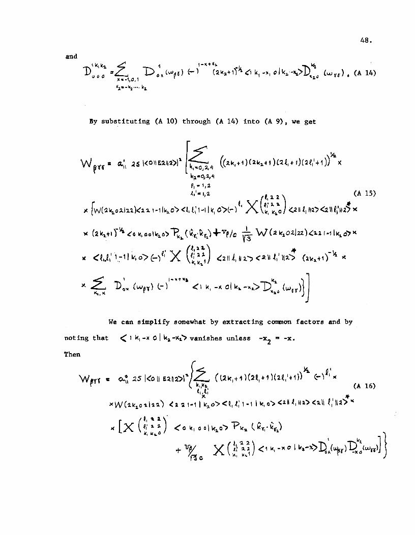
48.
and
!y substituting (A 10) through (A 14) into (A 9), we get
We can simplify somewhat by extracting common factors and by
noting that < 1 k, -l< 0 I k1 -X2.'> vanishes unless -x2 == -x.
Then
[4 .v~ U'
Wtty'f-= o..~, :zs i<ou E~Q:2.">\"' L...- (t21<,+1H:22,+1HH,'+1)) (-) 1 -< r k,,IC~ (A 16)
(,,.t; ~ .
x w ( 2.1< ~ o '2. 1 ~ 2.) < :a -2 1-1 1 ~<,. o > < t, ~: , - 1 1 ~<, o "> < 2. n ~ 1 11 :a.'> < ~ 11 t i 112 '> "
< o 1< 1 o o \ 1<2. o '> "'P '<2. ( k l', • ~r)
+ trp; X ( ~~ ~~) <• "· -• o I k,-~) D' l""rl 1:?"\w.,,l) 1 1(3c:. ~o~., 1<,.1 0)1. F XO )
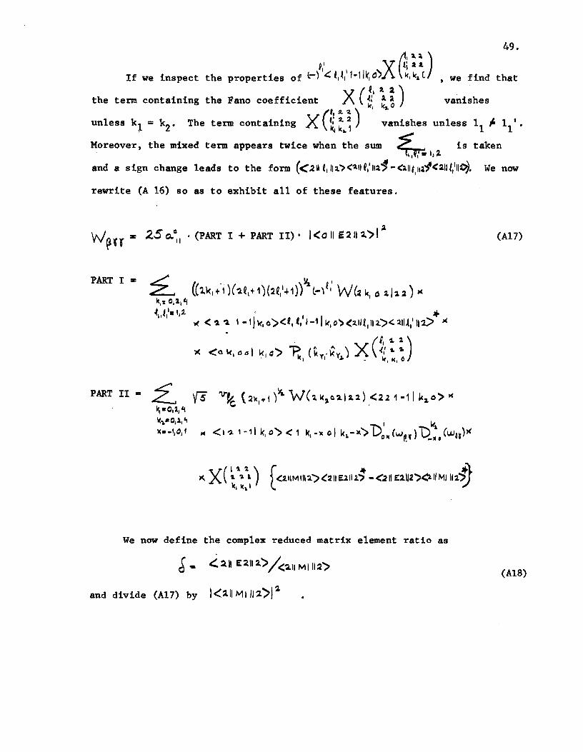
49. P' X f.;~;)
If we inspect the properties of l-)'.(;f,~,'1·11~.~") ~~,kz.t , we find that
X ( ~. a 2.) the term containing the Fano coefficient ~. ~ ~ vanishes
(f, fL '2.) ,.
unless k1 = k2• The term containing X ~ ~ .. ~ vanishes unless 11 1: 11' •
Moreover, the mixed term appears twice when the sum ~ ~IJ2.
is taken
and a sign change leads to the form (<.211 f1 ll:a."><'2.11 Qt'ua'1-ant1 u~-/<~lll1 1 11~. We now
rewrite (A 16) so as to exhibit all of these features.
PART I •
PART II = ~ ~1 •0,21 't \(~•01 a, 'I )(a.11Q1 1
We now define the complex reduced matrix element ratio as
~ • ~ ~~~ E:2.ll2.) /<:'411 Mlll:f>
and divide (A17) by l<2.h~IIIZ)j:a.
(A17)
(Al8)
Then, in PART I there are the following terms:
a) a mixed Ml-E2 term in {~ + 6*)/2 = Re{J), which is multiplied
by the LeGendre polynomial P&(k~·~~)
50.
b) pure Ml terms ( k'2.11MIII'l.':>l'-ll<z.IIMI•~'>I a. = 1 ) which are multiplied
by LeGendre polynomials P0 and P2 , and
c) pure E2 terms in 1$1~ which are multiplied by P0 , P2 , and P4 •
PART II contains a mixed term in -I. a ... _ ~ )j2 = - .J,.,..,( ~) • For convenience, we can also divide {Al7) by ~S o.~J~oiiE.2/12)/2..
times the coefficient of the k1 = O, 11 = 11
' - 1 term in PART I.
Henley and Jacobsoh~/ carried out the evaluation for the cascade,
and bbtained the result
~rr: W~uA2s tl.,~ l<oll Ellt2>12./<:,11Mlll2.)1' (-) v'3i; W (2 ~cal.u)XC•o\ ~))
= 1 + l~lt + (.0.25'0 f o. ':132([•+f) + ojo~~s /[ 11) "P~ l kr,o kr.)
2.
+ o. 32.':1/~ I"' ~ (k~ ·~,) - o. 2~S '1.?/c £ ~;f) k't( kJj w ~r._) (~· kw-.) •
"
{Al9)
As in the previous discussion, the k's are unit vectors in the direc-
tions of the outgoing particles. The reader will note that, according to the
definition above, the total probability for ~~t emission over all angles is
{A20)
APPENDIX B. ELECTRONICS
The basic electronics bas been discussed in Chapter IV. Here, we
treat several aspects of the system in more detail.
1. Fast Coincidence Circuitry.
Figure 1 - A. shows the fast coincidence circuitry with important
delays tAn' 1C , tw' and T. All other delays caused by connecting cables
and by the characteristics of the triggers, coincidence circuits, etc.
have been left out for the sake of simplicity. Only one ~ detector is
shown. Delay times, pulse widths, and energy thresholds are given in
Table 1 - A.
51.
Anode pulses corresponding to gamma energies greater than ~0.15
MeV cause the anode triggers to fire short logic pulses. Whenever anode
trigger pulses, delayed by tAn' are in coincidence with long logic pulses
from the Dy 12 triggers {which have thresholds corresponding to gamma
energies greater than ~0.50 MeV) the appropriate AnDy coincidence cir-
cuit fires. By putting an open cable, whose length corresponds to a ~/2
delay, on the AnDy A coincidence circuit, two short logic pulses ~ apart
are generated for each anode-dynode coincidence. AnDy B, operating in
normal fashion, fires once per anode-dynode coincidence. Timing is ar-
ranged so that an AnDy ~ pulse is in true coincidence with the first
AnDy A pulse and in false coincidence with the second. Because the delay
time 't is well outside the resolving time of the ~A t8 fast coincidence
circuit, the number of such false events that occur·within the course of
a run should statistically correspond to the number of accidental oAoa coincidences which are inseparable from true coincidences. This will be
true to the extent that the resolving time for the false pulse coinci-
dences is identical to the resolving time for the true pulse coincidences.
52.
Table 1 - A.
Typical Delays, Pulse Widths, and Thresholds
Pulse Width Trigger Threshold or Delay nsec (MeV)
tAn 25 An (A,:B) 0.15
'L 50 Dy 12 (A,:B) 0.50
T 325 Lowest Level o (A,!) 1.30 Storage
tw 29 Upper Level ~ (A,!) 0.95 Window
Dy 12 (A,!) 36
An (A,!) 6 Lower Level 0 (A,!) 0.55 Window
AnDy! 6 Lowest~. (A, :B) Disc. 0.10
AnDy A, AnDy A del. 6.6 Level
OArs 8 Lower Level Window ~ (A,!) Disc. 0.20
?AlPs 8.5 Upper Level ~ (A,!) Disc. 0.95
0 '{ ' rr del. 8.5 Disc.
Cor)~Alcrn~s 8
Wide A 50
Wide False oA Ys 50
53.
Figure 1 - A. Fast coincidence circuit and important delays.
~ DETECTOR rr-·---------, I ANODE A r7fr:m A I I TR TR I L:_ --- ___ j
I tAn
.____.-t ANDY A .,. c ,. ...... 'r ... _~-·--·
>; DETECTOR r~-----------;r
I ANODE I r7tNODE 1 I I TR 12 TR I ~--1-------'
t t-.------, ANDY 8 _
L......, c
ANDY A ANrJf I + AWIN A DELAYED 'r f ., ---IYa c ,. 'r/2
l T-'r
T
OPEN
COM· ...,.,
1I OR I WIDE MUlE. l OPEN
t ~ coa••MD
TO (YY) FALSE a .,_ _ _,I SLD. A R
D COINC. 'l ""• DETECTOR r ~.--:;,
FROM r1'f8 8
LG 8
TO PHA
FROM r1'f 8 A 1_
LG A
I
TO PHA
yy +yy DELAYED -r -y-y-
I ~L ...... ,1 -~ ltNERTER h I TR I .. ~
II LOWER I w~ ~ (YY)Ji c
TO (YY) J\ SLO. COINC.
LEVEL 1 r I TR R I I "\ I I c I LoWEST II
LEVEL i I TR tf'11ITI'I"t"-~ I ___ ~ fan
LG • LINEAR GATE
TR • TRIGGER
C • TWO-FOLD COINCDENCE
We have measured these resolving times and have seen that they differ
by less than one half per cent. Since the ratio of false to true coin-
cidences is ()(10-2). this would cause a negligible systematic error
in the determination of the interference term in the correlation.
Note the distinction (in the above) between true, accidental,
55.
and false coincidences. The first two are inseparable, but the last type
is manufactured by the circuitry in order to measure the second.
The false tA l 6 coincidence circuit fires only when a 'rA l6 coincidence
pulse is sufficiently late to be in coincidence with a subsidiary wide
pulse (delayed by tw) from AnDy A, i •. e., the false lrA o6 coincidence circuit
fires only when an AnDy ! pulse is in coincidence with the second
AnDy A pulse.
If a oo coincidence is present, any analysis of it will be sub-
jected to address modification or routing according to whether it was a
false or true coincidence by determining whether the second most signifi-
cant binary bit in the address register is 0 or 1. We have arranged this
address modification so that the false oA~ pulses are advanced four .
groups in the pulse height analyzer storage unit. A total of sixteen
groups is available in the multichannel analyzer. We have observed the
effect of routing which precedes pulse height analysis on that analysis
and found the areas under our photopeaks to be affected by less than one
part in 10-4 •
A second measure of accidental events is provided by the oA~B
coincidence circuit,which sends two pulses, separated by 1C , to the ,PA(~~)
fast coincidence circuit for every OA Oe (or delayed '(ArB ) coincidence.
These separated pulses are denoted '! o and o ~ delayed. Since the
short logic pulses which correspond to 0.20 MeV -:6 Ep..::;; 0.95 MeV are
effectively delayed 't + tA" • a true pA O't coincidence will give rise
56.
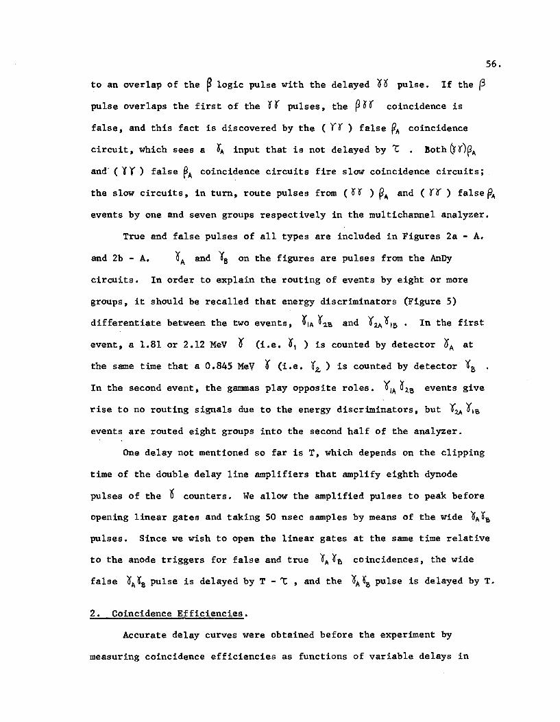
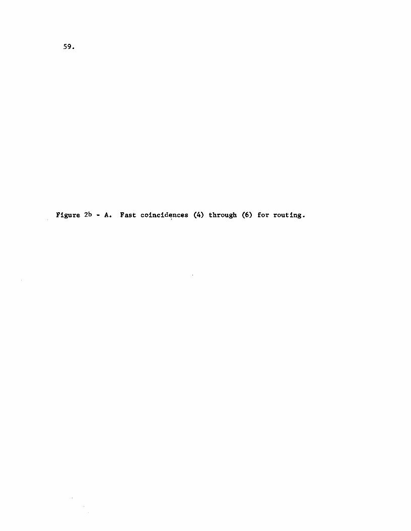
to an overlap of the ~ logic pulse with the delayed o ~ pulse. If the ~
pulse overlaps the first of the 0 r pulses' the p ~ r coincidence is
false, and this fact is discovered by the ( Yr ) false pA coincidence
circuit, which sees a oA input that is not delayed by 't . Both ~ r)~A
and ( Y '( ) false ~A coincidence circuits fire slow coincidence circuits;
the slow circuits, in turn, route pulses from ( ~ r ) ~A and ( (([ ) false ~A
events by one and seven groups respectively in the multichannel analyzer.
True and false pulses of all types are included in Figures 2a - A.
and 2b - A. 0 A and Y8 on the figures are pulses from the AnDy
circuits. In order to explain the routing of events by eight or more
groups, it should be recalled that energy discriminators (Figure 5)
differentiate between the two events, OIA ¥-:ta and ¥2A 018 • In the first
event, a 1.81 or 2.12 MeV ~ (i.e. ~1 ) is counted by detector OA at
the same time that a 0.845 MeV 0 (i.e. 'l'2..) is counted by detector ¥8 •
In the second event, the gammas play opposite roles. 01A ~2.6 events give
rise to no routing signals due to the energy discriminators, but o2A 0,8 events are routed eight groups into the second half of the analyzer.
One delay not mentioned so far is T, which depends on the clipping
time of the double delay line amplifiers that amplify eighth dynode
pulses of the ~ counters. We allow the amplified pulses to peak before
opening linear gates and taking 50 nsec samples by means of the wide OA~a
pulses. Since we wish to open the linear gates at the same time relative
to the anode triggers for false and true oA ~B coincidences, the wide
false OA ~8 pulse is delayed by T - 't , and the OA ~8 pulse is delayed by T.
2. Coincidence Efficiencies.
Accurate delay curves were obtained before the experiment by
measuring coincidence efficiencies as functions of variable delays in

57.
Figure 2a - A. Fast coincidences (1) through (3) for routing.
L= 50 nanoseconds. t = 10 nanoseconds. Table '
applies to cases (1) through (6) inclusive.
( I ) TRUE YY
t-T-l ~---v-· v--
v ~Ya--y
(3) TRUE ~ (YY)
~
---v ~ >a ---v yy --v-v-fl(A OR 8) y ~ (YY) y
(2) FALSE YY
v v v
IF ROUTE
(I) BUT NOT (3), OORI NOT (4)
(2) BUT NOT un. NOT (8) 4 OR 12
IQR2 (3) AND ( I )
9 OR 10
(4) AND ( I ) 3 OR 7 II OR 15
( 5) OR (6) 5 OR 8 - AND (2) 13 OR 14
59.
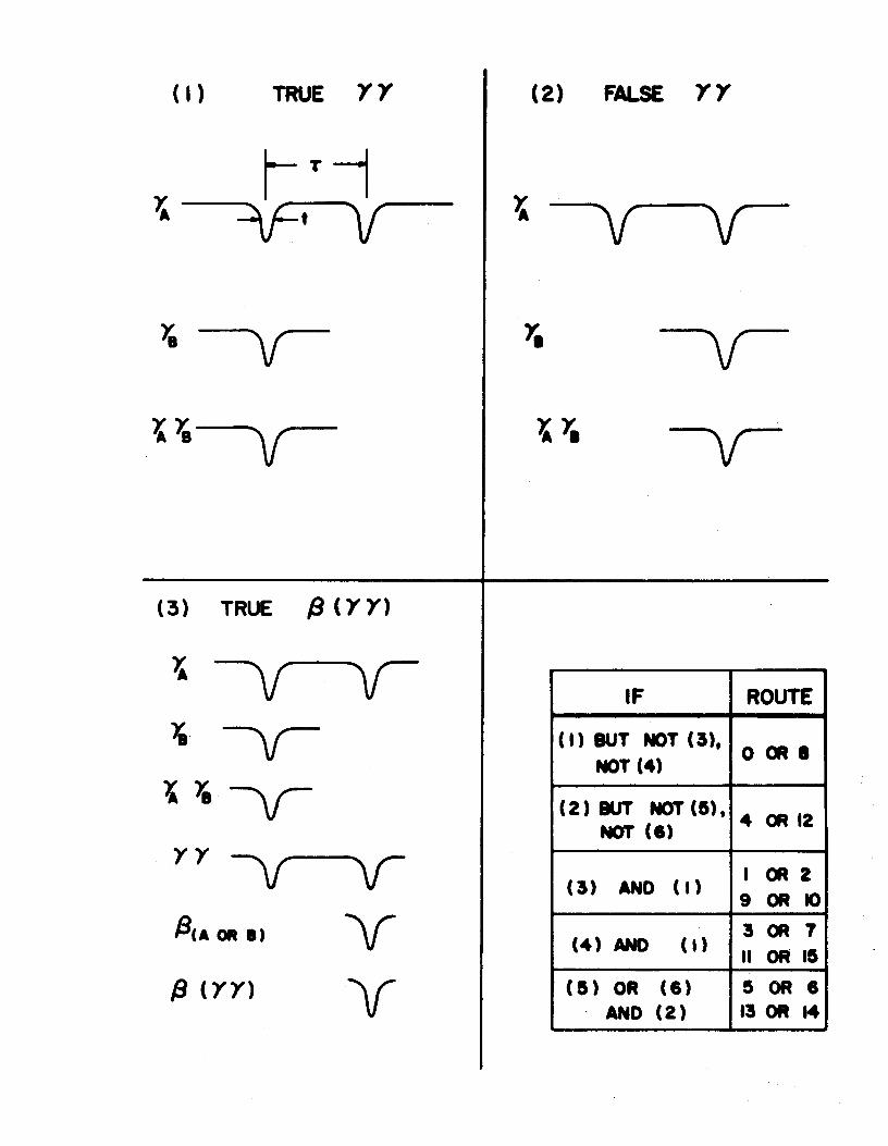
Figure 2b - A. Fast coincidences (4) through (6) for routing.
YA v ·Ya -v .YA·Ya ----v-'YY
BAORB ---v ~~'rn v . (4) FALSE ~ (Yr)
YA v Ya v-
lyA Ya v-Y7
/JAOR 8 --v· /J·(YY) v- (&) fJ ·( FALSE r.y )
.,. Ya -v (6) fj { FALSE y Y)
'7A·Ya -v YY
61.
the system. Periodically during the experiment we checked the coincidence
efficiencies to make sure that our circuits continued to operate at the
same points on the delay curves within 0.7 nsec. In order to obtain
accurate measurements of coincidence efficiencies we tested each important
coincidence circuit with one input pulse at least twice as wide as normal
and compared the performance using the wide input with normal performance.
This was done, in practice, by inserting a parallel coincidence circuit,
which was fed the altered input, into the system. Fast coincidences in
the normally operating circuit were registered as fast coincidences in
the "wide" circuit, but any coincidences in the wide circuit which
failed to register as fast coincidences in the normal circuit showed that
the normal circuit was not completely efficient. By making use of the
analyzer routing, we tested coincidence efficiencies in this fashion to 4 four parts in 10 •
3. Miscellaneous Tests.
As a check on the stability of the 0 counters and amplifiers,
we printed out coincidence pulse height spectra from the photomultiplier
tubes before and after each run, observed the photopeak positions, and
adjusted the threshold settings of the triggers in the gamma energy dis-
criminators whenever necessary. From time to time, the levels of the
beta discriminators were also checked using two conversion electron
sources, Bi207 and cs 137 , and suitable pulse attenuators. During the
course of each run logic pulses were scaled from various triggers and
coincidence circuits. Any gross malfunctions, e.g., a trigger that
latched or double-fired, could be quickly observed by means of the
scalers.

62.
APPENDIX C. DATA PROCESSING
Here we present a detailed description of the data analysis and
show the results for a typical run in Table 2-A.
1. Correcting for Accidental Coincidences.
Multichannel analyzer displays for Run #47 are exhibited in
Figures 3a - A. through 3d - A. If we assume false coincidence spectra
to correspond to accidentals of various types, then from the data stored
in the first half of the analyzer, we get
(A21)
Accidental " v - !=" F - ~ + 15' + 'G'_ IJ lA 0 2.e - '(lA - 'f2s- C!.J '¢:V I_IO /
F and T stand for false and true coincidences, the subscripts indicate
the particle observed and the detector that detected it, and the circles
stand for corresponding groups in the multichannel analyzer. From the
data stored in the second half of the analyzer, we obtain numbers of true
0 \B 0 :2.A ~A triples. true o,B 02A doubles' true ~le, 02A ~B triples and
accidental 018 ~:<A doubles. The forms are the same, except that each
circled number in (A21) is increased by eight, e.g.
63.
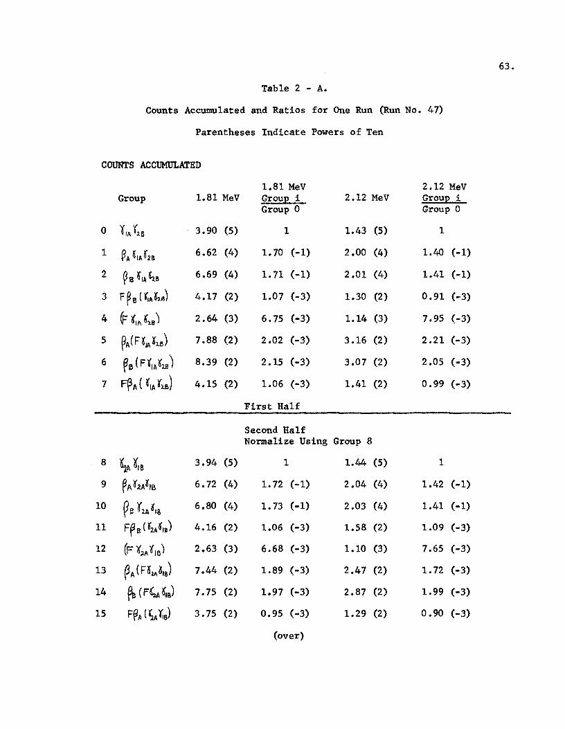
Table 2 - A.
Counts Accumulated and Ratios for One Run (Run No. 47)
Parentheses Indicate Powers of Ten
COUNTS ACCUMULATED
1.81 MeV 2.12 MeV Group 1.81 MeV GrouE i 2.12 MeV GrouE i
Group 0 Group 0
0 ¥,~ r.:ts 3.90 (5) 1 1.43 (5) 1
1 PA~,Ar2s 6.62 (4) 1.70 (-1) 2.00 (4) 1.40 (-1)
2 ~g ~lA ~1.8 6.69 (4) 1.71 (-1) 2.01 (4) 1.41 (-1)
3 F ~B ( f,A~:u~) 4.17 (2) 1.07 (-3) 1.30 (2) 0.91 (-3)
4 f '(If>.. ''l.B) 2.64 (3) 6. 75 (-3) 1.14 (3) 7.95 (-3)
5 ~A ( F t,A l2.6) 7.88 (2) 2.02 (-3) 3.16 (2) 2.21 (-3)
6 ~e ( F(IA ole) 8.39 (2) 2.15 (-3) 3.07 (2) 2.05 (-3)
7 F~A ( (,A rl.e.) 4.15 (2) 1.06 (-3) 1.41 (2) 0.99 (-3)
First Half
Second Half Normalize Using Group 8
8 01A tiB 3.94 (5) 1 1.44 (5) 1
9 ~A t2.A~IB 6. 72 (4) 1. 72 (-1) 2.04 (4) 1.42 (-1)
10 ~ e '( lA K'~~~ 6.80 (4) 1. 73 (-1) 2.03 (4) 1.41 (-1)
11 F~e n2A~IB) 4.16 (2) 1.06 (-3) 1.58 (2) 1.09 (-3)
12 (F ¥'-A (16) 2.63 (3) 6.68 (-3) 1.10 (3) 7.65 (-3)
13 ~A (nlll~ls) 7.44 (2) 1.89 (-3) 2.47 (2) 1.72 (-3)
14 ~ (f~~IQ) 7.75 (2) 1.97 (-3) 2.87 (2) 1.99 (-3)
15 F@A (~A ¥;8) 3.75 (2) 0.95 (-3) 1.29 (2) 0.90 (-3)
(over)
64.
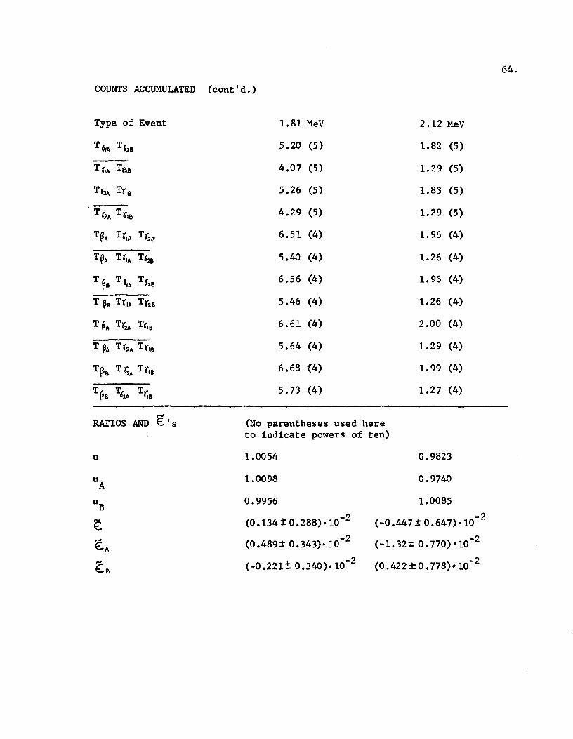
COUNTS ACCUMULATED (cont'd.)
Type of Event 1.81 MeV 2.12 MeV
T 41A Tr.2a 5.20 (5) 1.82 (5)
Tt,, Tr,.a 4.07 (5) 1.29 (5)
Tt2A Tt,s 5.26 (5) 1.83 (5)
TtlA Tr,e 4.29 (5) 1.29 (5)
T~,. Tr,A Tt;B 6.51 (4) 1.96 (4)
T~A Tt1,. Tt28 5.40 (4) 1.26 (4)
T Ty @e ll Tr1.a 6.56 (4) 1.96 (4)
T ~~ T(IA Trn 5.46 (4) 1.26 (4)
T Q,. TrlA Tt18 6.61 (4) 2.00 (4)
T ~A T 't:2.A T t 18 5.64 (4) 1.29 (4)
T~e. T ~ Tr18 6.68 '{4) 1.99 (4)
T T T Pa ~lA r.a 5.73 (4) 1.27 (4)
..... RATIOS AND E. I s (No parentheses used here
to indicate powers of ten)
u 1.0054 0.9823
UA 1.0098 0.9740
u'B 0.9956 1.0085
€ (0.134 ± 0.288)·10-2 (-0.447 ± 0.647)·10 -2
€_A (0.489± 0.343)• 10-2 (-1.32± 0.770)•10-2
.... £~
+ -2 (-0.221- 0.340)· 10 (0.422 ±0. 778)•10-2
65.
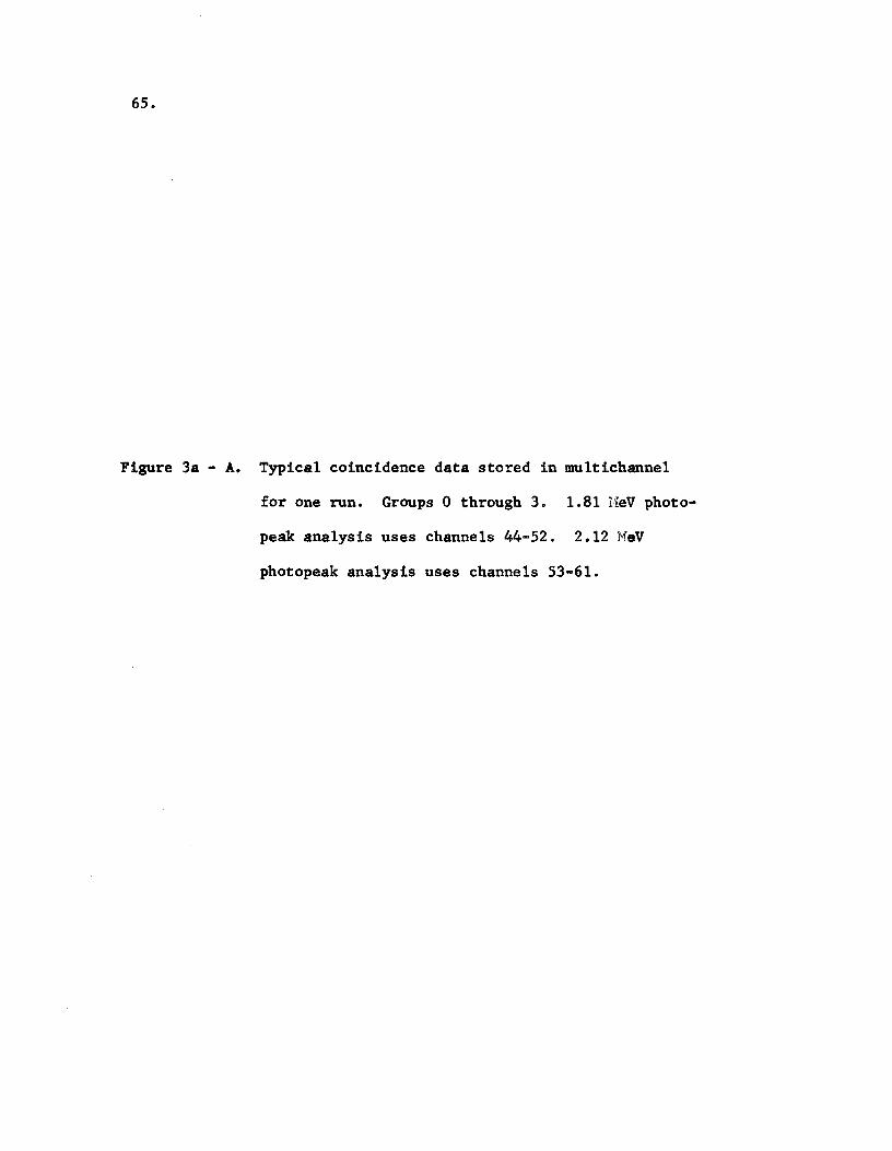
Figure 3a - A. Typical coincidence data stored in multichannel
for one run. Groups 0 through 3. 1.81 !::leV photo-
peak analysis uses channels 44-52. 2.12 !1eV
photopeak analysis uses channels 53-61.
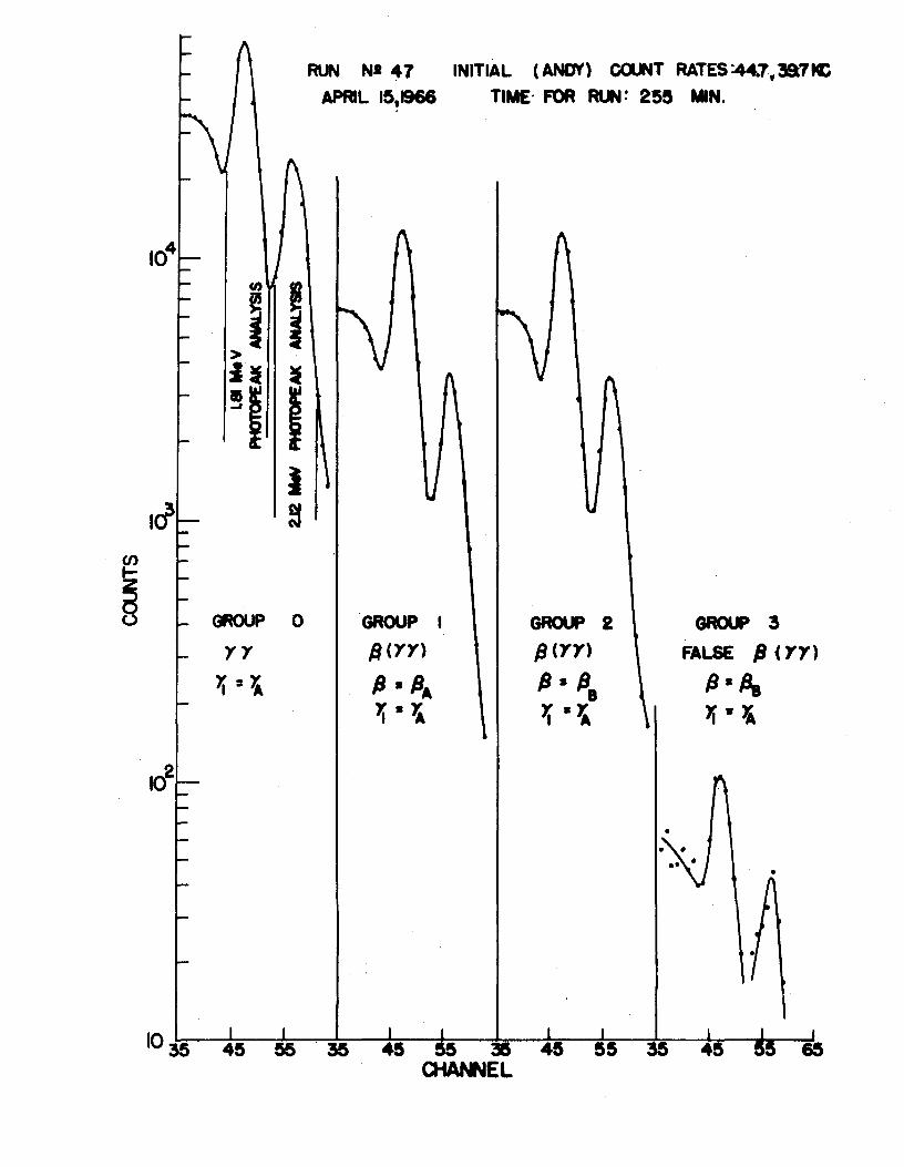
RUN Nl .. 7 INITIAL (ANDY) ca.t4T RATES =44.7 ;!87KC APRIL 15,1966 TIME· FOR ~: 255 MIN.
(I) I ; > :1~ • !I I
j ~
CJ) .... g GROUP 0 GROUP I GROUP 2 GROUP 3 yy /3 (YY) fJ (YY) FALSE fJ ( YY)
'!=l fJ • /JA IJ•IJ. a fJ •!Ja 'i·~ Ji·~ Ji•l
•
•
67.
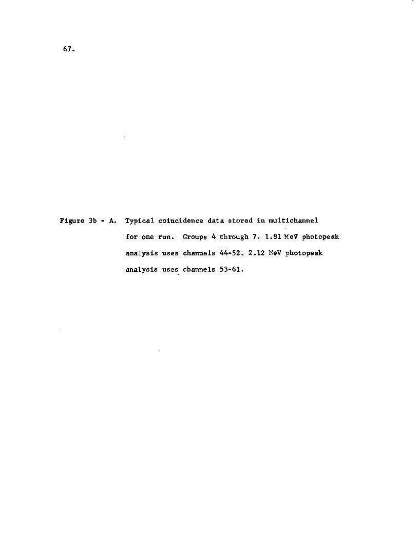
Figure 3b - A. Typical coincidence data stored in multichannel
for one run. Groups 4 through 7. 1.81 MeV photopeak
analysis uses channels 44-52. 2.12 MeV photopeak
analysis uses channels 53-61.
•
GROUP ~•4+1 GROlP 6 • 4+2
S (FaLSE Y S (FaLSE Y Y)
S•ll. l[ •1 S•/Ja ~·~
• •
• • • • •
35 CHANNEL
•
•
GROUP 7
FaLSE S ( Y Y )
S•!J,. >i•'A
• • • 4~ ss. e

69.
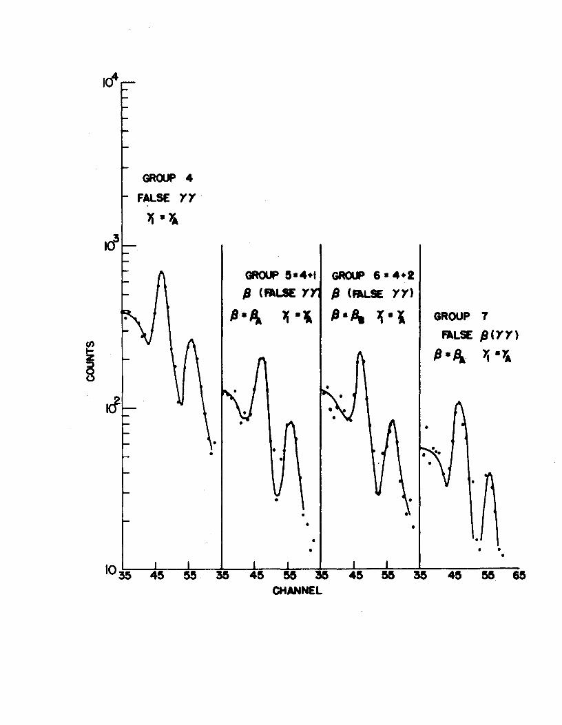
Figure 3c - A. Typical coincidence data stored in multichannel
for one run. Groups 8 through 11. 1.81 MeV
photopeak analysis uses channels 42-50. 2.12 MeV
photopeak analysis uses channels 51-59.
j I !J (\1
'""' 1rf (\1
~ g GROUP 8
yy
)j=>a
lcf
(jR()U) 9•8•1 GROlP 10• 8•2 /3 (YY)
/3. ~ 'i·>a
•
3& a4A*EL
fj(YY)
/3 ·~ 8
'J•Ya
GROUP II• 8+3 FALSE IJ ·( YY)
/3 •f\ )j•Ya
•
•
71.
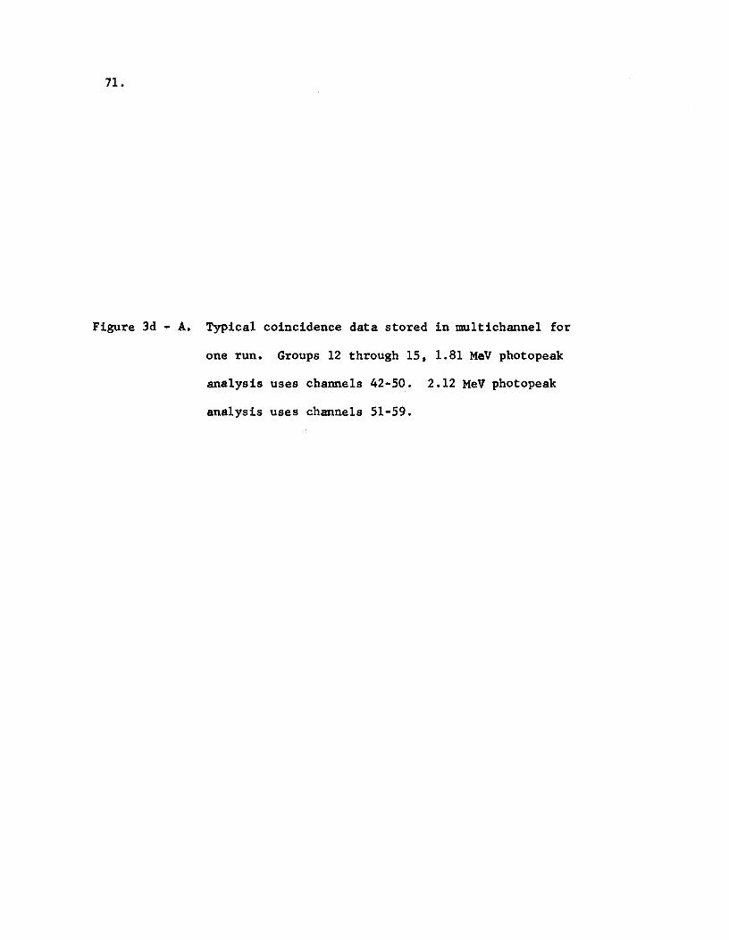
Figure 3d - A. Typical coincidence data stored in multichannel for
one run. Groups 12 through 15, 1.81 MeV photopeak
analysis uses channels 42-50. 2.12 MeV photopeak
analysis uses channels 51-59.
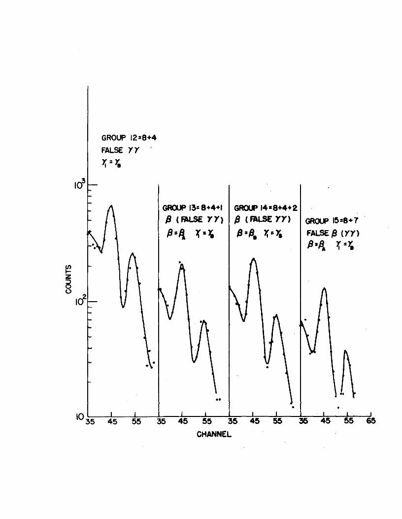
~ z a 0
GROUP 12=8+4
FALSE YY r.=r. I I
•
GRClJP 13= 8+4+1 /l (~ YY)
P•li ~-~
••
GROlF14•8+4+2 fl (~LSE YY)
/J =fl. Yes >I
•
•
GROlP 15 =8+ 7
FALSE /l (YY) D 11 D Y.=Y. ,_, ~ I I
•
35 45 55 35 55 35 CHANNEL
73.
We denote by FFF those accidental events in which all particles
come from different nuclei. ~ecause FFF's are counted twice in each
(false '('( ) ~ group and once in each ~( r r ) group and once in each
( lr) false ~ group, we add 2 X FFF in the expressions above. Accord-
ing to measurements and calculations, the numbers of FFF coincidences of
various types can be calculated for each run by using the stored data.
For example
(A22) @ +0+® +®+®- (® +®+®)
c:f (t) is a slowly varying fUnction of time whose value at the
beginning of each run (t = 0) is 1.0 and whose value at t= oo is ~ 1.33.
Since the number of FFF's was less than 0.01% of the TTT's for most runs,
we used ~ '1- = 1.0 in correcting the data. ~ecause the FFF's were the same ,....
fractions of TTT's, errors in € due to approximations in FFF's were
negligible.
2. Separation of 1.81 and 2.12 MeV Photopeaks.
Nine channels (310 keV) on either side of the valley between the
photopeaks were chosen for data analysis. Peaks and valleys were taken . 56
from inspection of groups @and ~ • We compared the Mn gamma spectra
with superimposed ce144 and Y88 spectra (with prominent ·2.18 and 1.84
MeV transitions) and obtained the following prescriptions for separating
the Mn56 photopeaks:
(T T T} = ((TTT ),-~r - {;•(TTT) P~~~.1)/(l- {1 { 2 ) I·•' ,,e1 (A23)
For the first half of the analyzer f 1 = 0.873, f 2 = 0.129.
For the second half f 1 = 0.751, f2 = 0.126.
f'.J ,...
3. Calculation of E:. and ~E.st from Data. ,...
We found u and E:. for each run according to the equations of
Chapter II. (Eqns. (9) and (10) )
,... r~. The statistical error in e ' denoted ~~ is given by
d(st - * (.t,_ Uucf )~ The ~Ut are the fractional errors in each of the four TTT's.
For example
4. Normalization Using '( '( Coincidences.
74.
(A24)
(A25)
(A26)
For the case in which double coincidences are used for normaliza-
tion (Eqns •. (13) - (16) ) . uA = (•'(lA Trls T~A / T'C'IA Tr.ts) • ( Ta-2A T.,..a / T~~ Ty•s T(3J Ua: (-rrls'TrlATf8 / Tr,e Tr2.J· ( Tr22 Tr,A /Tt"J.aTt,A Tp~)
(A27)
~
€. A (B) '='
75.
Photopeak separation takes the same form as (A23). Error analysis is
complicated by ~0 's. Since some groups enter both doubles and triples
expressions, careful attention must be paid to the analysis. Statistical
r~ and errors (I '"'A st
terms.
~gs are seen to be square roots of sums of thirty-two It
BIBLIOGRAPHY
1. J. H. Christenson, J. W. Cronin, V. L. Fitch, and R. Turlay,
Phys. Rev. Letters 13, 138 (1964).
2. J. Bernstein, G. Feinberg, and T. P. Lee, Phys. Rev. 139, B1650
(1965).
3. s. P. Lloyd, Phys. Rev. 81, 161 (1951).
4. T. D. Lee and C. N. Yang, Brookhaven National Laboratory Report
!NL - 443, 1957 (unpublished)
5. E. M. Henley and B. A. Jacobsohn, Phys. Rev. 111, 225 (1959);
E. M. Henley and B. A. Jacobsohn, Phys. Rev. 111, 234 (1959).
6. P. Stichel, z. Physik, !2Q, 264 (1958).
7. v. DeSabbata, Nuovo Cimento 21, 659 (1961);
V. DeSabbata, Nuovo Cimento 21, 1058 (1961).
8. E. Fuschini, v. Gadjokov, c. Maroni, and P. Veronesi, Nuovo Cimento
33, 709, (1964);
E. Fuschini, V. Gadjokov, C. Maroni, and P. Veronesi, Nuovo Cimento
~' 1309 (1964).
9. P. Dagley, M. A. Grace, J. Gregory, and J. Hill, Proc. Roy. Soc.
(London) 250, 550 (1959).
10. F. R. Metzger and w. B. Todd, Phys. Rev. 92, 904 (1953).
11. N. Levine, H. Frauenfelder, and A. Rossi, Z. Physik 151, 241 (1958).
12. L. Rosenfeld, Oriented Nuclei (Copenhagen,_ 1959).
13. E. M. Henley and B. A. Jacobsohn, Phys. Rev. Letters 16, 706 (1966).
76.
VITA
Martin Henry Garell was born on January 4, 1939 in Brooklvn.
New York. where he attended Brooklyn Technical High School, graduating
in 1956. He then entered Princeton University and received his Bachelor
or Arts degree in Physics in 1960. While attending Princeton, he
wrote his Bachelor's thesis under Professor R. Sherr. He enrolled at
the University of Illinois as a graduate student in the fall of 1960,
having received a National Science Foundation Cooperative Fellowship
for that year. During his stay at Illinois, he served as a teaching
assistant in undergraduate physics courses for two years and as a
research assistant for five years. He received his Master of Sciences
degree in 1962 and is a member of the American Physical Society.
77.