Embed Size (px)
Citation preview
A STEADY STATE AND QUASI-STEADY INTERFACE
BETWEEN THE GENERALIZED FLUID SYSTEM
SIMULATION PROGRAM AND THE SINDA/G
THERMAL ANALYSIS PROGRAM
Paul Schallhorn and Alok Majumdar
Sverdrup Technology, Inc.
Huntsville, Alabama
Bruce Tiller
NASA Marshall Space Flight Center
MSFC, Alabama
ABSTRACT
A general purpose, one dimensional fluid flow code is currently being interfaced with the thermal analysis
program S1NDA/G. The flow code, GFSSP, is capable of analyzing steady state and transient flow in a
complex network. The flow code is capable of modeling several physical phenomena including
compressibility effects, phase changes, body forces (such as gravity and centrifugal) and mixture
thermodynamics for multiple species. The addition of GFSSP to SINDA/G provides a significant
improvement in convective heat transfer modeling for SINDA/G. The interface development is conducted
in multiple phases. This paper describes the first phase of the interface which allows for steady and quasi-
steady (unsteady solid, steady fluid) conjugate heat transfer modeling.
INTRODUCTION
Accurate conjugate heat transfer predictions for complex situations require both proper modeling of the
solid and flow networks and realistically modeling the interaction between these networks. Proper
modeling of the solid network can be easily performed using either classical analytical techniques or with
established numerical model tools, such as SINDA/G. Proper modeling of the flow network, however,
requires a numerical tool that account for multiple different flow paths, a variety of flow geometries, an
ability to predict flow reversal, the ability to account for compressibility effects and ability to predict phase
change.
THERMAL CODE
SINDA/G 1 (S_S_S__stemsImproved Numerical Differencing Analyzer / G__aski) is a code that solves the diffusion
equation using a lumped parameter approach. The code was developed as a general purpose thermal
analysis program which uses a conductor-capacitor network to represent a physical situation; however,
SINDA can solve other diffusion type problems. The code consists of two components: a preprocessor and
a library. The library consists of a series of subroutines necessary to solve a wide variety of problems. The
preprocessor converts the input model deck into a driver FORTRAN source code, complies and links with
the library, then executes the model and generates an output file. One of the main advantages of S1NDA
https://ntrs.nasa.gov/search.jsp?R=20020050398 2018-08-31T04:31:08+00:00Z
overotherthermalcodesis thatit acceptsFORTRANstatements,developedbytheuser,intheinputdeckwhichallowtheusertotailorthecodeto suitaparticularproblem.It is thisabilitytoaddFORTRANcodingtotheS1NDAinputdeckwhicheasilyallowsforaninterfacewithothercodes,specificallyinthecaseathand,ageneralpurposefluidnetworkflowcode.
FLUID CODE
CODE
The Generalized Fluid System Simulation Program 2 (GFSSP) was developed for the Marshall Space Flight
Center's Propulsion Laboratory for the purpose of calculating pressure and flow distribution in a complex
flow network associated with secondary flow in a liquid rocket engine turbopump. The code was developed
to be a general purpose, one-dimensional flow network solver so that generic networks could be modeled.
Capabilities of the GFSSP are summarized below:
Modeling flow distributions in a complex network;
Modeling of compressible and incompressible flows;
Modeling real fluids via embedded thermodynamic and thermophysical properties routines and
tables;
Mixing calculation of real fluids;
Phase change calculation of real fluids;
Axial thrust calculations for turbopumps;
Calculation o f buoyancy driven flows;
Calculation of both steady and unsteady flows (both boundary conditions and geometry can vary
with time);
Choice of first or second law approach to solving the energy equation.
The GFSSP uses a series of nodes and branches to define the flow network. Nodes are positions within the
network where fluid properties (pressure, density, etc.) are either known or calculated. Branches are the
portions of the flow network where flow conditions (geometry, flow rate, etc.) are known or calculated.
The code contains 18 various branch options to model different geometries. These branch options include
classical pipe flow with and without end losses, flow with a loss coefficient, non-circular duct, thick orifice,
thin orifice, square expansion, square reduction, face seal, labyrinth seal, valves and tees, pump using pump
characteristics, pump using horsepower and efficiency, and a Joule-Thompson device.
The GFSSP has additional options including the ability to model gravitational effects, rotation, fluid
mixture, a turbopump assembly, the ability to add mass, momentum and heat sources at any appropriate
point in the model, and the ability to model multidimensional flow (two and three dimensional flow field
calculation).
The GFSSP uses a finite volume approach with a staggered grid. This approach is commonly used in
computational fluid dynamics schemes (Patankar 3, Patankar and Karki4).
OVERVIEW OF SOLID/FLUID INTERFACE
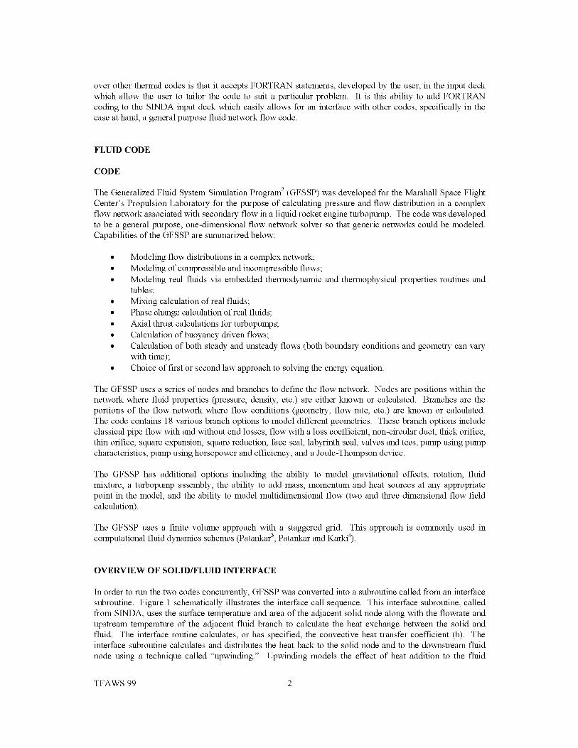
In order to run the two codes concurrently, GFSSP was converted into a subroutine called from an interface
subroutine. Figure 1 schematically illustrates the interface call sequence. This interface subroutine, called
from S1NDA, uses the surface temperature and area of the adjacent solid node along with the flowrate and
upstream temperature of the adjacent fluid branch to calculate the heat exchange between the solid and
fluid. The interface routine calculates, or has specified, the convective heat transfer coefficient (h). The
interface subroutine calculates and distributes the heat back to the solid node and to the downstream fluid
node using a technique called "upwinding." Upwinding models the effect of heat addition to the fluid
TFAWS 99 2
manifesting downstream of the point of the addition, from a bulk flow perspective. This technique is
commonly used in CFD codes to model fluid inertia. Figure 2 illustrates the convective heat transfercalculation scheme.
SINDA/GCalls InterfaceSubroutine InVARIABLES1
Figure 1 S1NDA - GFSSP Interface
........ _ ................ _ ............... / QFi -- -QSi
Legend
--Fluid Internal Node F_ --Solid Internal Node
tin-q--Fluid Boundary Node-- Solid Boundary Node
-- Fluid Branch
Figure 2: Convective Heat Transfer Scheme Within The S1NDA - GFSSP Interface
From the point of view of the two codes involved, therefore, only heat sources/sinks are added at discretenodes and these heat sources/sinks are updated with every S1NDA iteration.
The interface is generalized so that the solid and fluid models can have different levels of discretization,resulting in three different scenarios: multiple solid nodes for a given fluid branch, one solid node for agiven fluid branch, and one solid node for multiple fluid branches. These three scenarios are illustrated in
Figure 3.
TFAWS 99 3
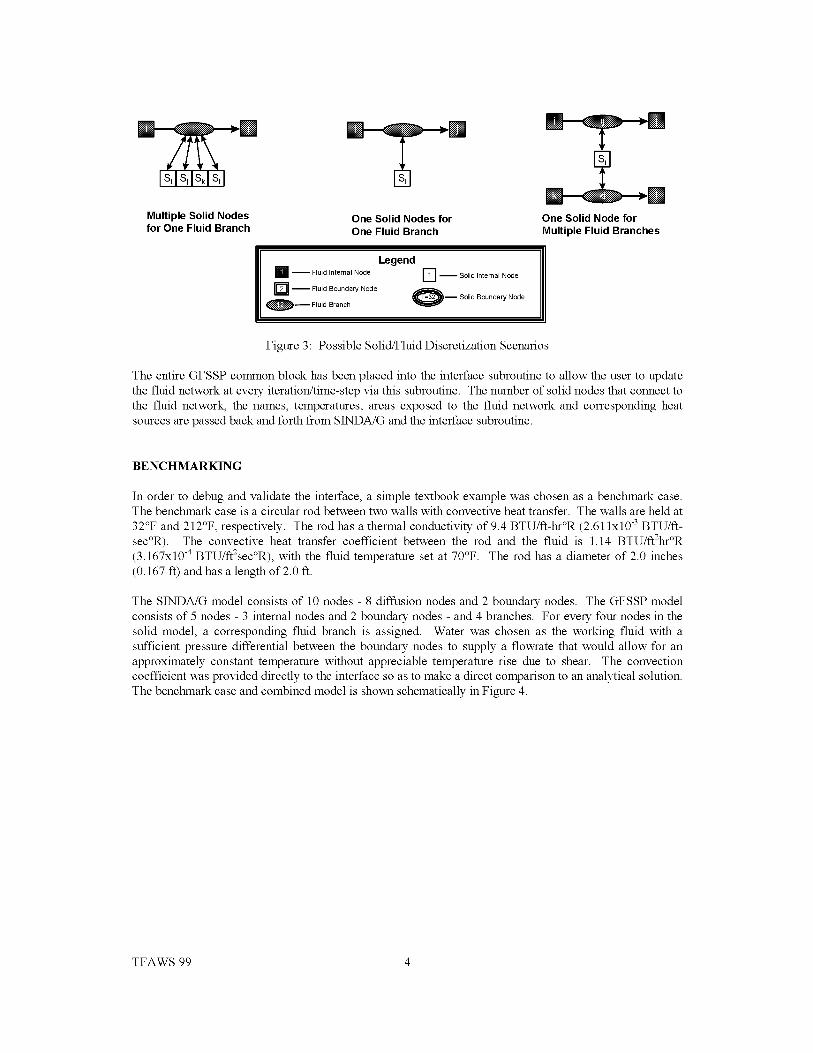
Multiple Solid Nodesfor One Fluid Branch
One Solid Nodes forOne Fluid Branch
Legend
-- Fluid Internal Node [] -- Solid Internal Node
tin-q--Fluid Boundary Node-- Solid Boundary Node
_ Fluid Branch
One Solid Node for
Multiple Fluid Branches
Figure 3: Possible Solid/Fluid Discretization Scenarios
The entire GFSSP common block has been placed into the interface subroutine to allow the user to update
the fluid network at every iteration/time-step via this subroutine. The number of solid nodes that connect to
the fluid network, the names, temperatures, areas exposed to the fluid network and corresponding heat
sources are passed back and forth from S1NDA/G and the interface subroutine.
BENCHMARKING
In order to debug and validate the interface, a simple textbook example was chosen as a benchmark case.The benchmark case is a circular rod between two walls with convective heat transfer. The walls are held at
32°F and 212°F, respectively. The rod has a thermal conductivity of 9.4 BTU/ft-hr°R (2.61 lxl0 -3 BTU/ft-
sec°R). The convective heat transfer coefficient between the rod and the fluid is 1.14 BTU/ft2hr°R
(3.167x10 -4 BTU/ft2sec°R), with the fluid temperature set at 70°F. The rod has a diameter of 2.0 inches
(0.167 ft) and has a length of 2.0 ft.
The SINDA/G model consists of 10 nodes - 8 diffusion nodes and 2 boundary nodes. The GFSSP model
consists of 5 nodes - 3 internal nodes and 2 boundary nodes - and 4 branches. For every four nodes in the
solid model, a corresponding fluid branch is assigned. Water was chosen as the working fluid with a
sufficient pressure differential between the boundary nodes to supply a flowrate that would allow for an
approximately constant temperature without appreciable temperature rise due to shear. The convection
coefficient was provided directly to the interface so as to make a direct comparison to an analytical solution.
The benchmark case and combined model is shown schematically in Figure 4.
TFAWS 99 4
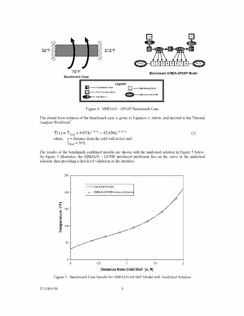
32°F
70°F
Benchmark Case
212°F
1121314151617181-
Benchmark SINDA-GFSSP Model
Legend
I_-- Fluid Internal Node [] -- Solid Internal Node
-- Fluid Boundary Node 1___Solid Boundary Node
I_D_ Fluid Branch
Figure 4: S1NDA/G - GFSSP Benchmark Case
The closed form solution of the benchmark case is given in Equation 1, below, and derived in the ThermalAnalysis Workbook 5.
T(x) = Zfluid -I- 4.653e 1714× - 42.650e 1.714x (1)
where, x = distance from the cold wall in feet and
Tfluid = 70°F.
The results of the benchmark combined models are shown with the analytical solution in Figure 5 below.As Figure 5 illustrates, the S1NDA/G - GFSSP interfaced prediction lies on the curve of the analyticalsolution, thus providing a first level validation of the interface.
25O
o
E
200
150
100
5O
--Analytical Solution
SINDA/G-GFSSP Interfaced Solution
I I I
05 1 15
Distance from Cold Wall (x, ft)
Figure 5: Benchmark Case Results for SINDA/G-GF SSP Model with Analytical Solution
TFAWS 99 5
ADDITIONAL TEST CASES
In order to exercise the interface between S1NDA/G and GFSSP, three additional test cases were identified
which exploit different aspects of the interface.
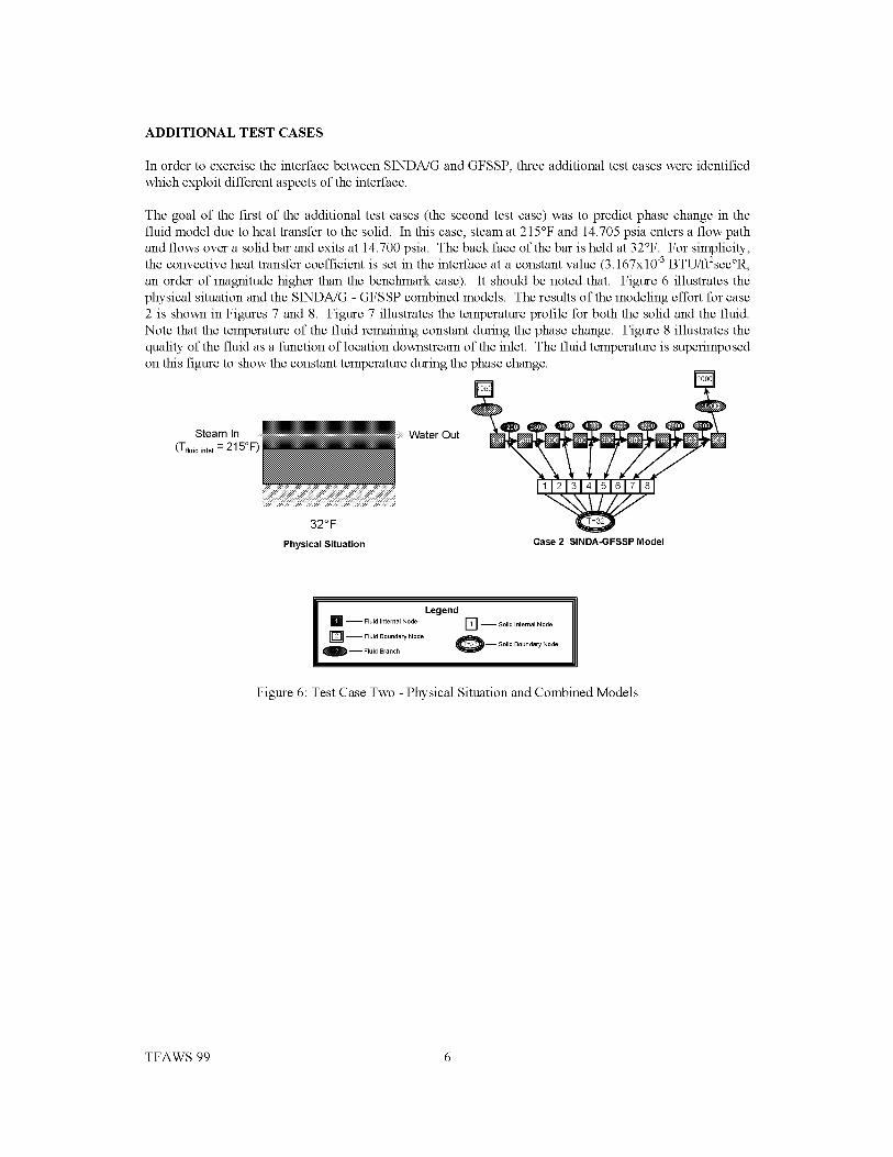
The goal of the first of the additional test cases (the second test case) was to predict phase change in the
fluid model due to heat transfer to the solid. In this case, steam at 215°F and 14.705 psia enters a flow path
and flows over a solid bar and exits at 14.700 psia. The back face of the bar is held at 32°F. For simplicity,
the convective heat transfer coefficient is set in the interface at a constant value (3.167x10 -3 BTU/ft2sec°R,
an order of magnitude higher than the benchmark case). It should be noted that. Figure 6 illustrates the
physical situation and the S1NDA/G - GFSSP combined models. The results of the modeling effort for case
2 is shown in Figures 7 and 8. Figure 7 illustrates the temperature profile for both the solid and the fluid.
Note that the temperature of the fluid remaining constant during the phase change. Figure 8 illustrates the
quality of the fluid as a function of location downstream of the inlet. The fluid temperature is superimposed
on this figure to show the constant temperature during the phase change.
Steam In ..................................... Water Out
(T_u,d inlet 215 F)
32°F
Physical SituationCase 2 SINDA-GFSSP Model
Legend
I_-- Fluid Internal Node [] -- Solid Internal Node
Q_ Fluid Boundary Node
-- Solid Boundary Node
-- Fluid Branch
Figure 6: Test Case Two - Physical Situation and Combined Models
TFAWS 99 6
220
200
A180
o
"_ 160
Q,,E
140I--
120
IO0
Fluid
Solid
i i i i i i i i
1 2 3 4 5 6 7 8
Position (Relative to Solid Node Numbers)
Figure 7: Test Case Two - Temperature vs. Location for both Solid & Fluid Models
1 250
>,
1
O
200
I.I.0.7 o
0.6 150
0.5 _.
E0.4 1001_
"O.1
0.3 '_1I.I.
0.2 _ Quality 50
Temperature0.1
0 ,0
100 200 300 400 500 600 700 800 900
Node Number
Figure 8: Test Case Two - Fluid Quality vs. Location
The goal of the second of the additional test cases (the third test case) was to control the area of an orificeusing a temperature supplied by S1NDA/G. In this case, a metal bar is bounded by two fluid streams (onecold, the other hot) in steady state operation as illustrated in Figure 9, below. The bar is 0.25 feet thick,with a thermal conductivity of 18.8 BTU/ft-hr°R (5.22x10 -3 BTU/ft-sec°R). The bar has been descretized
into 35 solid nodes. The cold fluid stream consists of water entering at boundary node 1 with boundaryconditions of 70°F and 45.5 psia, and exiting at boundary node 8 with a boundary pressure of 45.0 psia.
TFAWS 99 7
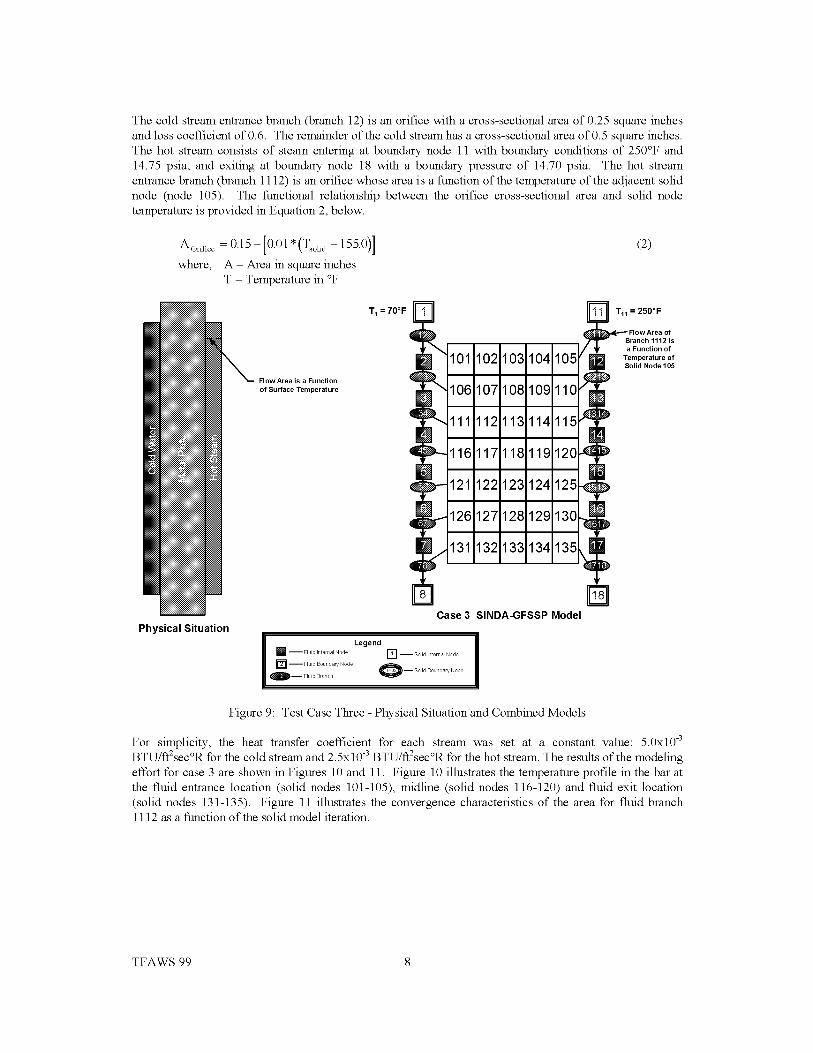
Thecoldstreamentrancebranch(branch12)isanorificewithacross-sectionalareaof0.25squareinchesandlosscoefficientof0.6.Theremainderofthecoldstreamhasacross-sectionalareaof0.5squareinches.Thehotstreamconsistsof steamenteringatboundarynode11withboundaryconditionsof 250°Fand14.75psia,andexitingatboundarynode18withaboundarypressureof 14.70psia.Thehotstreamentrancebranch(branch1112)isanorificewhoseareaisafunctionofthetemperatureoftheadjacentsolidnode(node105).Thefunctionalrelationshipbetweentheorificecross-sectionalareaandsolidnodetemperatureisprovidedinEquation2,below.
Ao_i_ce=0.15+[0.01*(Tsolid155.0)]where,A=Areainsquareinches
T=Temperaturein°F
T1 = 70°F D
FlowArea is a Function
of Surface Temperature
101 102 103 104 105
106 107 108 109 110
(2)
T11 = 250°F
Branch 1112 is
a Function of
Temperature of
Solid Node 105
111 112113114115
116 117 118 119 120
121 122 123 124 125
126127128129130
131 132133134135
Physical SituationCase 3 SINDA-GFSSP Model
Figure 9: Test Case Three - Physical Situation and Combined Models
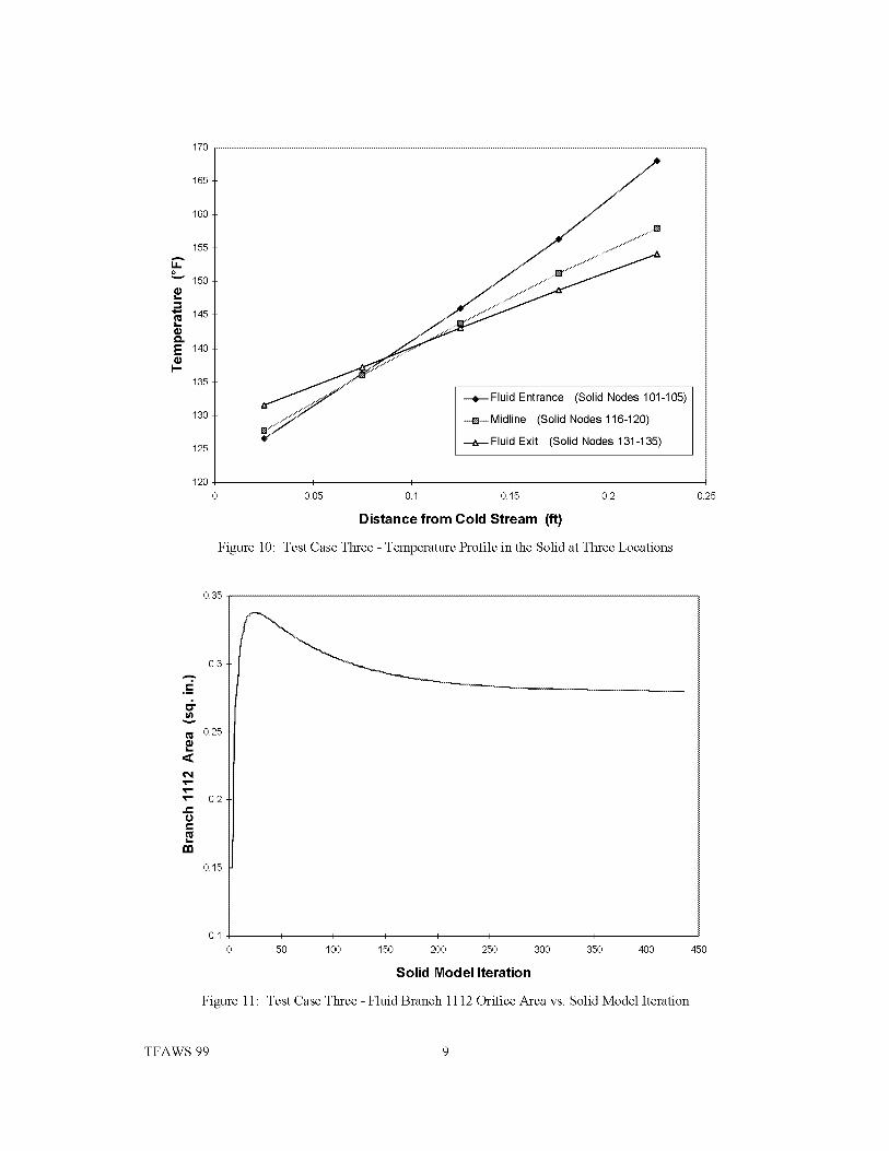
For simplicity, the heat transfer coefficient for each stream was set at a constant value: 5.0x10 -3
BTU/ft2sec°R for the cold stream and 2.5x10 -3 BTU/ft2sec°R for the hot stream. The results of the modelingeffort for case 3 are shown in Figures 10 and 11. Figure 10 illustrates the temperature profile in the bar atthe fluid entrance location (solid nodes 101-105), midline (solid nodes 116-120) and fluid exit location
(solid nodes 131-135). Figure 11 illustrates the convergence characteristics of the area for fluid branch1112 as a function of the solid model iteration.
TFAWS 99 8
o
EI--
17o
165
16o
155
15o
145
14o
135
13o
125
12o
-105)
_ ................... ,...m....Midline (Solid Nodes 116-120)
Fluid Exit (Solid Nodes 131-135)
I I I I
0.05 0.1 0.15 0.2
Distance from Cold Stream (ft)
Figure 10: Test Case Three - Temperature Profile in the Solid at Three Locations
0.25
0.35
,m
6-&
m
0.3
0.25
0.2
o.15
o.1 I I I I I I I I
50 1O0 150 200 250 300 350 400 450
Solid Model Iteration
Figure 11 Test Case Three - Fluid Branch 1112 Orifice Area vs. Solid Model Iteration
TFAWS 99 9
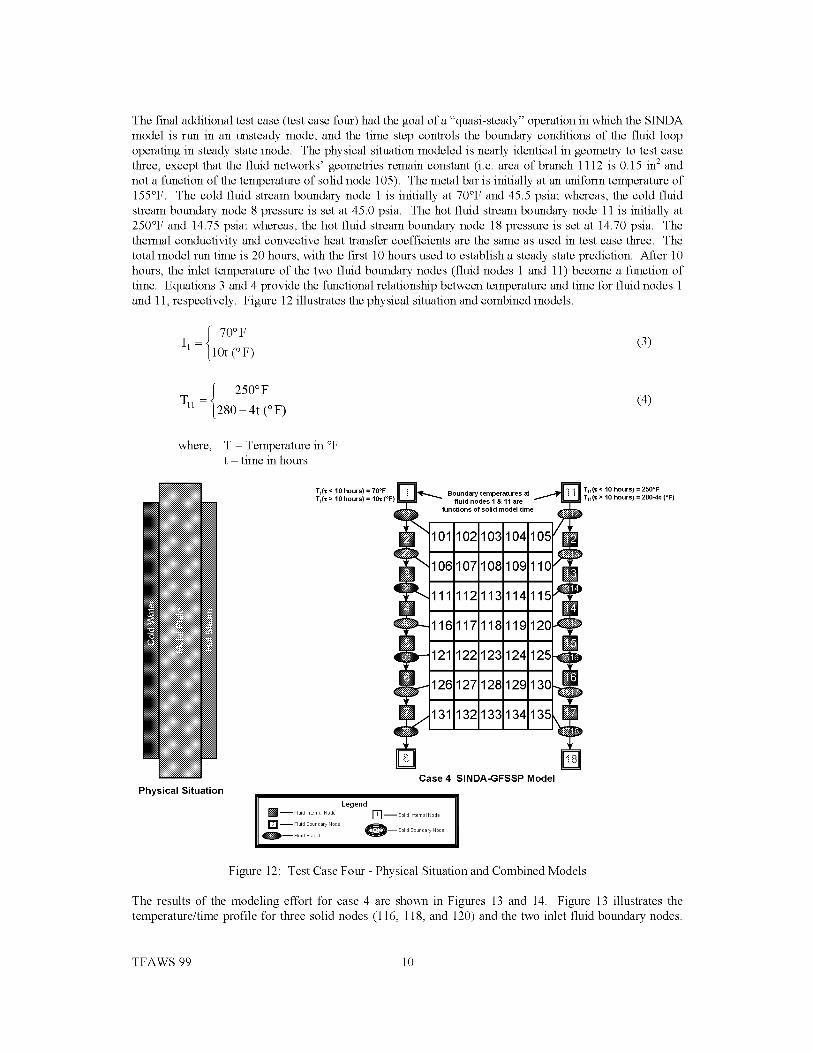
The final additional test case (test case four) had the goal of a "quasi-steady" operation in which the S1NDA
model is run in an unsteady mode, and the time step controls the boundary conditions of the fluid loopoperating in steady state mode. The physical situation modeled is nearly identical in geometry to test casethree, except that the fluid networks' geometries remain constant (i.e. area of branch 1112 is 0.15 in2 andnot a function of the temperature of solid node 105). The metal bar is initially at an uniform temperature of
155°F. The cold fluid stream boundary node 1 is initially at 70°F and 45.5 psia; whereas, the cold fluidstream boundary node 8 pressure is set at 45.0 psia. The hot fluid stream boundary node 11 is initially at250°F and 14.75 psia; whereas, the hot fluid stream boundary node 18 pressure is set at 14.70 psia. The
thermal conductivity and convective heat transfer coefficients are the same as used in test case three. Thetotal model run time is 20 hours, with the first 10 hours used to establish a steady state prediction. After 10hours, the inlet temperature of the two fluid boundary nodes (fluid nodes 1 and 11) become a function oftime. Equations 3 and 4 provide the functional relationship between temperature and time for fluid nodes 1
and 11, respectively. Figure 12 illustrates the physical situation and combined models.
= _ 70 °FT1 _10t (oF)
(3)
Yll =
250°F
280 - 4t (° F) (4)
where, T = Temperature in °Ft = time in hours
TI( < 10 hours) = 70°F
TI( > 10 hours) = 10 (°F)
_J H T11( < 10 hours) = 250°FBoundary temperatures at_ _ TII(E > 10 hours) = 2804 (°F)fluid nodes I & 11 are
/
functions of solid model time--
101 102 103 104 105
106 107 108 109 110
111112113114115
116 117 118 119 120
121 122123124 125
126127128129130
131 132 133 134 135
PhysicalSituationCase4 SINDAGFSSPModel
Figure 12: Test Case Four - Physical Situation and Combined Models
The results of the modeling effort for case 4 are shown in Figures 13 and 14. Figure 13 illustrates thetemperature/time profile for three solid nodes (116, 118, and 120) and the two inlet fluid boundary nodes.
TFAWS 99 10
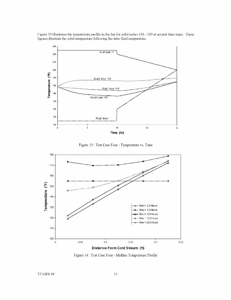
Figure14illustratesthetemperatureprofileinthebarforsolidnodes116- 120atseveraltimesteps.Thesefiguresillustratethesolidtemperaturefollowingtheinletfluidtemperature.
26O
240
220
200
o180
160
Q.
E 140
h-
120
100
"1
Fluid Node 11 _"_
Solid Node 120 __......¢... _
Solid Node 118 _-_
Solid Node 116
Fluid Node 1
5 10 15
Time (hr)
2O
180
Figure 13: Test Case Four - Temperature vs. Time
170
160
o 150
140
(2.E
130t--
120
110
100 I I I I
0.05 0.1 0.15 0.2
Distance From Cold Stream (ft)
Figure 14: Test Case Four - Midline Temperature Profile
0.25
TFAWS 99 11
IMPLEMENTATION STATUS
To date, the interface subroutine has been developed to allow for modeling of steady state flow networks
with steady or unsteady solid modeling. Development is currently underway for fully unsteady modeling in
which the time step for the fluid model may be different than that of the solid model.
CONCLUSIONS
A general purpose fluid network code has successfully been interface with a general purpose thermal
analysis code for steady state flow models and both steady and unsteady thermal models. A benchmark
case was identified, combined models were constructed and executed. The predictions from the combined
benchmark models provided an accurate prediction of the temperature profile in the solid when compared to
the analytical, closed form solution. Three additional cases demonstrated fluid phase prediction and control
of the fluid model by the solid model's information via the interface subroutine. A status of the
implementation was also provided.
ACKNOWLEDGEMENTS
The authors wish to acknowledge the contributions of Mr. Randy Lycans of Sverdrup Technology and Dr.
Barry Battista of Tec-Masters.
This work was performed for the George C. Marshall Space Flight Center under contract NAS8-40386,Task Directive 661-007.
REFERENCES
1. Behee, R.: SINDA/G User's Guide, Version 1.81, Network Analysis, Inc., 1998.
2. Majumdar, A.K.; Bailey, J.W.; Schallhom, P.A.; Steadman, T. :A Generalized Fluid System Simulation
Program to Model Flow Distributions in Fluid Networks, (User's Manual) SvT Report No. 331-201-
97-005, NASA MSFC Contract No. NAS 8-40836, October 1997.
3. Patankar, S., Numerical Heat Transfer and Fluid Flow, Hemisphere Publishing Co., New York, 1980.
4. Patankar, S., Karki, K., Documentation of COMPACT-2D Version 3.1, (User's Manual) Innovative
Research, Inc., 1993.
5. Owen, J.W. (ed.): ThermalAnalysis Workbook, NASA TM-103568, p.1-3-2, January 1992.
TFAWS 99 12


![[2] the Aerodynamics of Hovering Insect Flight I. the Quasi-Steady Analysis](https://img.pdfslide.us/doc/110x75/577d21f01a28ab4e1e963cee/2-the-aerodynamics-of-hovering-insect-flight-i-the-quasi-steady-analysis.jpg)