400 Commonwealth Drive, Warrendale, PA 15096-0001 U.S.A. Tel: (724) 776-4841 Fax: (724) 776-5760

SAE TECHNICALPAPER SERIES 2000-01-3563

Lap Time Simulation: Comparison of SteadyState, Quasi- Static and TransientRacing Car Cornering Strategies

Blake Siegler, Andrew Deakin and David CrollaThe School of Mech. Eng., The University of Leeds

Reprinted From: Proceedings of the 2000 SAE MotorsportsEngineering Conference & Exposition

(P-361)

Motorsports Engineering Conference & ExpositionDearborn, Michigan

November 13-16, 2000

The appearance of this ISSN code at the bottom of this page indicates SAE’s consent that copies of thepaper may be made for personal or internal use of specific clients. This consent is given on the condition,however, that the copier pay a $7.00 per article copy fee through the Copyright Clearance Center, Inc.Operations Center, 222 Rosewood Drive, Danvers, MA 01923 for copying beyond that permitted by Sec-tions 107 or 108 of the U.S. Copyright Law. This consent does not extend to other kinds of copying such ascopying for general distribution, for advertising or promotional purposes, for creating new collective works,or for resale.

SAE routinely stocks printed papers for a period of three years following date of publication. Direct yourorders to SAE Customer Sales and Satisfaction Department.

Quantity reprint rates can be obtained from the Customer Sales and Satisfaction Department.

To request permission to reprint a technical paper or permission to use copyrighted SAE publications inother works, contact the SAE Publications Group.

No part of this publication may be reproduced in any form, in an electronic retrieval system or otherwise, without the prior writtenpermission of the publisher.

ISSN 0148-7191Copyright 2000 Society of Automotive Engineers, Inc.

Positions and opinions advanced in this paper are those of the author(s) and not necessarily those of SAE. The author is solelyresponsible for the content of the paper. A process is available by which discussions will be printed with the paper if it is published inSAE Transactions. For permission to publish this paper in full or in part, contact the SAE Publications Group.

Persons wishing to submit papers to be considered for presentation or publication through SAE should send the manuscript or a 300word abstract of a proposed manuscript to: Secretary, Engineering Meetings Board, SAE.

Printed in USA

All SAE papers, standards, and selectedbooks are abstracted and indexed in theGlobal Mobility Database

2000-01-3563

Lap Time Simulation: Comparison of Steady State,Quasi- Static and Transient Racing Car

Cornering Strategies

Blake Siegler, Andrew Deakin and David CrollaThe School of Mech. Eng., The University of Leeds

Copyright © 2000 Society of Automotive Engineers, Inc.

ABSTRACT

Considerable effort has gone into modelling theperformance of the racing car by engineers inprofessional motorsport teams. The teams are usingprogressively more sophisticated quasi-static simulationsto model vehicle performance. This allows optimisationof vehicle performance to be achieved in a more cost andtime effective manner with a more efficient use ofphysical testing.

Racing cars are driven at the limit of adhesion in the non-linear area of the vehicle’s handling performance.Previous simulations have modelled the transientbehaviour by approximating it with a quasi-static modelwhich ignores dynamic effects, for example yawdamping. This paper describes a comparison betweendifferent cornering modelling strategies, including steadystate, quasi-static and transient. The simulation resultsfrom the three strategies are compared and evaluated fortheir ability to model actual racing car behaviour.

INTRODUCTION

The use of a Lap Time Simulation (LTS) package isbeneficial and complements the numerous tools (CAD,FEA, CFD) available to the teams and designers. LTSpackages allow the team to gain a significant advantageover their competitors. This is achieved by simulating thevehicle negotiating the circuit (which they may havenever visited) in any of its possible setup combinations tooptimise the vehicle’s performance, before they reach thecircuit or even before they build the vehicle. LTSpackages allows an expensive vehicle to be modelled atits limit of adhesion, without risk of the vehicle beingdamaged or injury to the driver, as is the case with tracktesting. Moreover, it has a use during the initial designphase after which parameters, such as the centre ofgravity position, cannot be changed. The vehicle canthen be produced so that the fundamental designparameters are close to the optimum values.

To simulate a full lap the path of the vehicle is normallysplit up into segments (for example every 1m) and ananalysis made of the vehicle at each segment point,using the external forces acting on the vehicle. This isnormally done as a simple quasi-static model, where thecircuit is idealised as a series of straights and constantradius turns. A commonly used method of finding thefastest lap time has been described by Milliken et al. [1].It involves using the corners as limiting factors for thesimulation. The maximum speed at which the vehicle cannegotiate all the corners is found (which is independentof the straight speeds), this gives the speed the vehicleenters and leaves all the straights. From this, thevehicle’s performance along the straights can then befound.

There are several methods by which the vehicle’sperformance in the corners can be modelled. This paperdescribes the construction and use of three vehiclemodelling strategies which are used to simulate a smallformula type racing car in two manoeuvres:

1. The first is a j-turn manoeuvre at constant forwardvelocity.

2. The second is the vehicle in the same j-turnmanoeuvre but where it is braking down from a highforward velocity to allow it to negotiate the corner(i.e. vehicle braking into a hairpin).

The three different vehicle modelling strategies used tofind the performance of the vehicle are as follows:

1. Steady state strategy.2. Quasi-static strategy.3. Transient strategy.

DEFINITIONS

m: Mass, kga: Centre of gravity distance from front axle, mb: Centre of gravity distance from rear axle, mCd: Aerodynamic coefficient of dragCl: Aerodynamic coefficient of liftFA: Frontal area of vehicle, m2

µµµµrr: Rolling resistance coefficientρρρρ: Air mass density, kg/m3

I: Second moment of area of vehicle, kgm2

A: Acceleration, m/s2

u: Forward velocity, m/sv: Lateral velocity, m/sr: Yaw velocity , rad/sF: Force, NM: Moment, NmN: Normal force on axle, ND: Drag force, Nαααα: Tyre slip angle, radδδδδ: Steered angle of tyre, radττττ: Iteration time constant, secondsx: variable of function f{x}g: Gravitational constant, m/s2

l: Wheelbase of car, msr: Longitudinal slip ratio at the tyre contact patch

SUBSCRIPTS - f: At front axler: At rear axlen: Number of iterationsx: In longitudinal directiony: In lateral direction

Axis System - the axis system used is the SAE standardvehicle and tyre axis system [2].

MODELLING RACING CAR BEHAVIOUR

The equations that are used to model the behaviour ofthe vehicle can come in many forms but most methodsare based on Newton’s Laws. These allow prediction ofthe acceleration of the vehicle due to the forces appliedto it. This is an efficient and effective method ofassessing the vehicle performance, as simple equationscan represent the vehicle in three axis and threerotational degrees of freedom.

To simulate the two different j-turn manoeuvres thevehicle’s path is split into two segments. The straightsegment where the vehicle is travelling in a straight lineand the cornering segment. It is modelled decelerating,from the maximum velocity reached on the straight, usinga basic quasi-static braking model, until it is travellingslow enough to allow it to negotiate the corner.

The simulation of the longitudinal acceleration behaviouruses a common method detailed by Gillespie [3]. Hesuggests that the vehicle’s braking behaviour can beidealised using a lumped mass model of the vehicle. Theacceleration of the vehicle can then be used to find thelongitudinal load transfer, using a moment calculation.Also the effect of aerodynamic lift can be calculated.

To accurately predict behaviour of a racing car, you needto be able to replicate the external forces acting on thevehicle. At low speeds the main external forces actingon the vehicle are generated by the tyres. Racing carsoperate at the peak of the tyre force curves, where theforce is greatest. The tyres therefore need to bemodelled as closely as possible, to allow accurateprediction of racing car The model must not onlyaccurately model tyre performance, but also the effect onresultant force, of changing the normal force at the tyrecontact patch.

The most commonly used tyre model for vehiclesimulation is based on an empirical approach, oftenreferred to as the Pacejka Magic Formula method [4].The braking force the tyre produces is a function of thelongitudinal slip ratio at the tyre contact patch (which isassumed to be held at the optimum value by the driver)and the normal force on that axle. Other importanteffects include aerodynamic and tyre drag losses, seeequation (1).

{ } xaerotyrerfx mADDNNsrfF =++= �4

,, (1)

where 2...21 uCFA

lhmA

lmgbN lf

xf ρ++= (2)

and 2...21 uCFA

lhmA

lmgaN lr

xr ρ+−= (3)

The effects of aerodynamic and tyre drag have beenfound by Dixon [5]. Where for each tyre the drag force isgiven in equation (4).

αµα cossin NFD rrytyre += (4)

And the total aerodynamic drag force is given in equation(5).

2...21 uCFAD daero ρ= (5)

In the cornering segment, the lateral accelerationperformance of the vehicle is modelled by assuming themass of the vehicle is concentrated at the vehicle’scentre of gravity, and a suitable value for the secondmoment of area is given to give a realistic yaw inertia andthus yaw response. Crolla [6] has shown that theequations of motion of the vehicle cornering can bederived from first principles, using a simple inertial axissystem, as shown in figure 1.

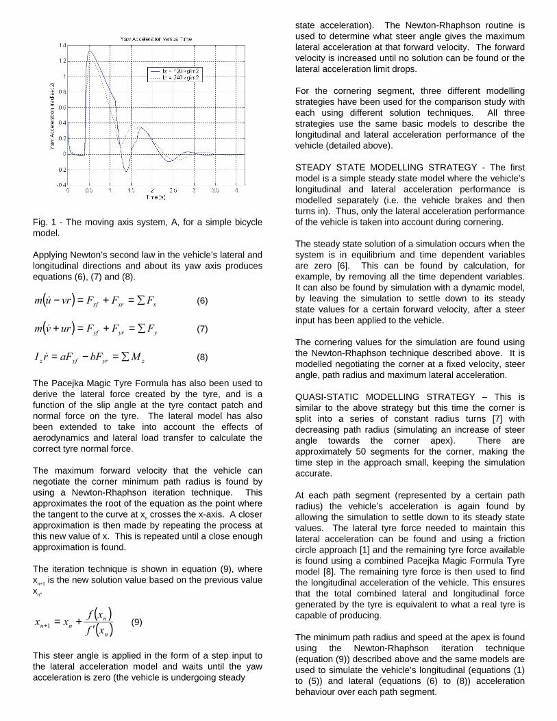
Fig. 1 - The moving axis system, A, for a simple bicyclemodel.

Applying Newton’s second law in the vehicle’s lateral andlongitudinal directions and about its yaw axis producesequations (6), (7) and (8).

( ) xxrxf FFFvrum �=+=−� (6)

( ) yyryf FFFurvm �=+=+� (7)

zyryfz MbFaFrI �=−=� (8)

The Pacejka Magic Tyre Formula has also been used toderive the lateral force created by the tyre, and is afunction of the slip angle at the tyre contact patch andnormal force on the tyre. The lateral model has alsobeen extended to take into account the effects ofaerodynamics and lateral load transfer to calculate thecorrect tyre normal force.

The maximum forward velocity that the vehicle cannegotiate the corner minimum path radius is found byusing a Newton-Rhaphson iteration technique. Thisapproximates the root of the equation as the point wherethe tangent to the curve at xn crosses the x-axis. A closerapproximation is then made by repeating the process atthis new value of x. This is repeated until a close enoughapproximation is found.

The iteration technique is shown in equation (9), wherexn+1 is the new solution value based on the previous valuexn.

( )( )nn

nn xfxf

xx′

+=+1 (9)

This steer angle is applied in the form of a step input tothe lateral acceleration model and waits until the yawacceleration is zero (the vehicle is undergoing steady

state acceleration). The Newton-Rhaphson routine isused to determine what steer angle gives the maximumlateral acceleration at that forward velocity. The forwardvelocity is increased until no solution can be found or thelateral acceleration limit drops.

For the cornering segment, three different modellingstrategies have been used for the comparison study witheach using different solution techniques. All threestrategies use the same basic models to describe thelongitudinal and lateral acceleration performance of thevehicle (detailed above).

STEADY STATE MODELLING STRATEGY - The firstmodel is a simple steady state model where the vehicle’slongitudinal and lateral acceleration performance ismodelled separately (i.e. the vehicle brakes and thenturns in). Thus, only the lateral acceleration performanceof the vehicle is taken into account during cornering.

The steady state solution of a simulation occurs when thesystem is in equilibrium and time dependent variablesare zero [6]. This can be found by calculation, forexample, by removing all the time dependent variables.It can also be found by simulation with a dynamic model,by leaving the simulation to settle down to its steadystate values for a certain forward velocity, after a steerinput has been applied to the vehicle.

The cornering values for the simulation are found usingthe Newton-Rhaphson technique described above. It ismodelled negotiating the corner at a fixed velocity, steerangle, path radius and maximum lateral acceleration.

QUASI-STATIC MODELLING STRATEGY – This issimilar to the above strategy but this time the corner issplit into a series of constant radius turns [7] withdecreasing path radius (simulating an increase of steerangle towards the corner apex). There areapproximately 50 segments for the corner, making thetime step in the approach small, keeping the simulationaccurate.

At each path segment (represented by a certain pathradius) the vehicle’s acceleration is again found byallowing the simulation to settle down to its steady statevalues. The lateral tyre force needed to maintain thislateral acceleration can be found and using a frictioncircle approach [1] and the remaining tyre force availableis found using a combined Pacejka Magic Formula Tyremodel [8]. The remaining tyre force is then used to findthe longitudinal acceleration of the vehicle. This ensuresthat the total combined lateral and longitudinal forcegenerated by the tyre is equivalent to what a real tyre iscapable of producing.

The minimum path radius and speed at the apex is foundusing the Newton-Rhaphson iteration technique(equation (9)) described above and the same models areused to simulate the vehicle’s longitudinal (equations (1)to (5)) and lateral (equations (6) to (8)) accelerationbehaviour over each path segment.

At present LTS packages find the cornering ability of thevehicle by using the quasi-static solution [9]. This allowsthe simulation to run quickly and efficiently, as acomplicated time dependent solution is not sought.

TRANSIENT MODELLING STRATEGY - In this strategya transient solution is sought. This is found when thevehicle is undergoing non-steady linear or rotationalaccelerations [5]. In reality, as the vehicle corners, it isnever in a steady state situation as the vehicle is alwaysaccelerating in a combination of the linear lateral,longitudinal or normal directions and/or the rotationalpitch, roll or yaw directions. The dynamic yaw responseof the vehicle and its effects on the overall results isexamined in the transient modelling strategy.

The transient simulation takes into account the responsetime of the vehicle in changing its attitude and direction oftravel. Consequently, complex transient simulations canbe performed which include the effect of dynamic yaw onthe model. Also the lateral and longitudinal weighttransfer effects (pitch and roll), as well as slip angleinduced tyre drag forces, are passed between thelongitudinal (equations (1) to (5)) and lateral (equations(6) to (8)) models, detailed above. Again a PacejkaMagic Force tyre model [8] is used to ensure that thecorrect combined tyre forces generated are applied.

As the vehicle corners it turns into the corner until itreaches its maximum steer angle and lateral accelerationat the corner apex. The maximum values at the apexwhich is applied to this model is found using the Newton-Rhaphson iteration technique (equation (9)) describedabove.

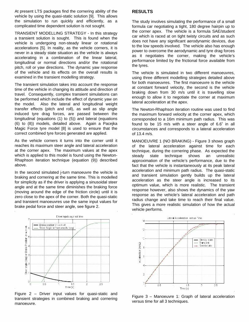
In the second simulated j-turn manoeuvre the vehicle isbraking and cornering at the same time. This is modelledfor simplicity as if the driver is applying a sinusoidal steerangle and at the same time diminishes the braking force(moving around the edge of the friction circle) until it iszero close to the apex of the corner. Both the quasi-staticand transient manoeuvres use the same input values forbrake pedal force and steer angle, see figure 2.

Figure 2 – Driver input values for quasi-static andtransient strategies in combined braking and corneringmanoeuvre.

RESULTS

The study involves simulating the performance of a smallformula car negotiating a tight, 180 degree hairpin up tothe corner apex. The vehicle is a formula SAE/studentcar which is raced at on tight twisty circuits and as suchdoes not have any significant aerodynamic devices, dueto the low speeds involved. The vehicle also has enoughpower to overcome the aerodynamic and tyre drag forcesas it negotiates the corner, making the vehicle’sperformance limited by the frictional force available fromthe tyres.

The vehicle is simulated in two different manoeuvres,using three different modelling strategies detailed abovefor both manoeuvres. The first manoeuvre is the vehicleat constant forward velocity, the second is the vehiclebraking down from 30 m/s until it is travelling slowenough to allow it to negotiate the corner at maximumlateral acceleration at the apex.

The Newton-Rhaphson iteration routine was used to findthe maximum forward velocity at the corner apex, whichcorresponded to a 16m minimum path radius. This wasfound to be 15 m/s with a steer angle of 6.6o in allcircumstances and corresponds to a lateral accelerationof 13.4 m/s.

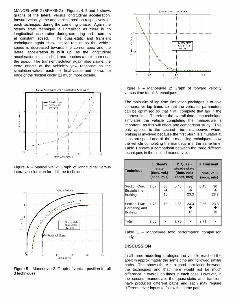
MANOEUVRE 1 (NO BRAKING) - Figure 3 shows graphof the lateral acceleration against time for eachtechnique, during the cornering phase. As expected thesteady state technique shows an unrealisticapproximation of the vehicle’s performance, due to thefact that the vehicle is instantaneously at its peak lateralacceleration and minimum path radius. The quasi-staticand transient simulation gently builds up the lateralacceleration as the steer angle is increased to itsoptimum value, which is more realistic. The transientresponse however, also shows the dynamics of the yawresponse as the vehicle’s lateral acceleration and pathradius change and take time to reach their final value.This gives a more realistic simulation of how the actualvehicle performs.

Figure 3 – Manoeuvre 1: Graph of lateral accelerationversus time for all 3 techniques.

MANOEUVRE 2 (BRAKING) - Figures 4, 5 and 6 showsgraphs of the lateral versus longitudinal acceleration,forward velocity time and vehicle position respectively foreach technique, during the cornering phase. Again thesteady state technique is unrealistic as there is nolongitudinal acceleration during cornering and it cornersat constant speed. The quasi-static and transienttechniques again show similar results as the vehiclespeed is decreased towards the corner apex and thelateral acceleration is built up, as the longitudinalacceleration is diminished, and reaches a maximum nearthe apex. The transient solution again also shows theextra effects of the vehicle’s yaw response as thesimulation values reach their final values and follows theedge of the ‘friction circle’ [1] much more closely.

Figure 4 – Manoeuvre 2: Graph of longitudinal versuslateral acceleration for all three techniques.

Figure 5 – Manoeuvre 2: Graph of vehicle position for all3 techniques.

Figure 6 – Manoeuvre 2: Graph of forward velocityversus time for all 3 techniques

The main aim of lap time simulation packages is to givecomparative lap times so that the vehicle’s parameterscan be optimised so that it will complete that lap in theshortest time. Therefore the overall time each techniquesimulates the vehicle completing the manoeuvre isimportant, as this will effect any comparison study. Thisonly applies to the second j-turn manoeuvre wherebraking is involved because the first j-turn is simulated atconstant speed and all three modelling techniques showthe vehicle completing the manoeuvre in the same time.Table 1 shows a comparison between the three differenttechniques in the second manoeuvre.

Technique

1. Steadystate

(time, vel.)(secs, m/s)

2. Quasi-steady state(time, vel.)(secs, m/s)

3. Transient

(time, vel.)(secs, m/s)

Section One:Straight lineBraking

1.07 30�

15

0.45 30�

23.3

0.45 30�

23.3

Section Two:Cornering andBraking

1.78 15 2.38 23.3�

15

2.36 23.3�

15

Total: 2.85 - 2.73 - 2.71 -

Table 1 – Manoeuvre two: performance comparisonstudy.

DISCUSSION

In all three modelling strategies the vehicle reached theapex in approximately the same time and followed similarpaths. This shows there is a good correlation betweenthe techniques and that there would not be muchdifference in overall lap times in each case. However, inthe second manoeuvre, the quasi-static and transienthave produced different paths and each may requiredifferent driver inputs to follow the same path.

Unfortunately no data logger data is available and adetailed comparison study with each of the differentsolution techniques with the actual vehicle’s performanceis not possible. However the overall performance of theactual vehicle has been measured under steady stateaccelerations. Table 2 shows a good correlation betweenwhat has been observed during vehicle testing andsimulated results.

Value MeasuredValue

SimulatedValue

Maximum Lateral Acc. onconstant radius steer pad test(10m path radius)

12.8 m/s2 13.4 m/s2

Steer Wheel Angle atMaximum Lateral Acc.(10m path radius)

Approx.60o

65o

Average Longitudinal Acc. infull stop from 40 ms-1

14.7 m/s2 14.9 m/s2

Table 2 – Measured and simulated overall performancevalues for 2000 Leeds University Formula SAE car.

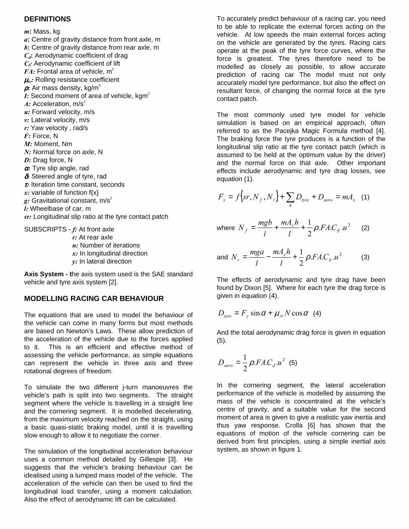
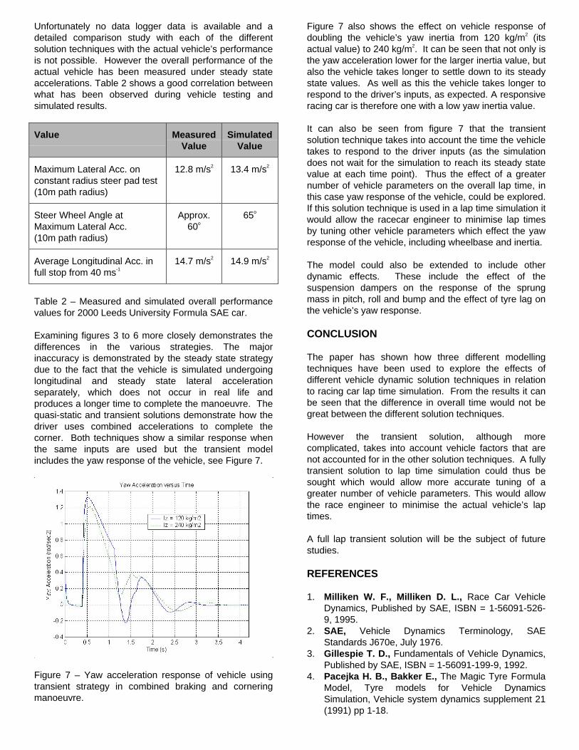
Examining figures 3 to 6 more closely demonstrates thedifferences in the various strategies. The majorinaccuracy is demonstrated by the steady state strategydue to the fact that the vehicle is simulated undergoinglongitudinal and steady state lateral accelerationseparately, which does not occur in real life andproduces a longer time to complete the manoeuvre. Thequasi-static and transient solutions demonstrate how thedriver uses combined accelerations to complete thecorner. Both techniques show a similar response whenthe same inputs are used but the transient modelincludes the yaw response of the vehicle, see Figure 7.

Figure 7 – Yaw acceleration response of vehicle usingtransient strategy in combined braking and corneringmanoeuvre.

Figure 7 also shows the effect on vehicle response ofdoubling the vehicle’s yaw inertia from 120 kg/m2 (itsactual value) to 240 kg/m2. It can be seen that not only isthe yaw acceleration lower for the larger inertia value, butalso the vehicle takes longer to settle down to its steadystate values. As well as this the vehicle takes longer torespond to the driver’s inputs, as expected. A responsiveracing car is therefore one with a low yaw inertia value.

It can also be seen from figure 7 that the transientsolution technique takes into account the time the vehicletakes to respond to the driver inputs (as the simulationdoes not wait for the simulation to reach its steady statevalue at each time point). Thus the effect of a greaternumber of vehicle parameters on the overall lap time, inthis case yaw response of the vehicle, could be explored.If this solution technique is used in a lap time simulation itwould allow the racecar engineer to minimise lap timesby tuning other vehicle parameters which effect the yawresponse of the vehicle, including wheelbase and inertia.

The model could also be extended to include otherdynamic effects. These include the effect of thesuspension dampers on the response of the sprungmass in pitch, roll and bump and the effect of tyre lag onthe vehicle’s yaw response.

CONCLUSION

The paper has shown how three different modellingtechniques have been used to explore the effects ofdifferent vehicle dynamic solution techniques in relationto racing car lap time simulation. From the results it canbe seen that the difference in overall time would not begreat between the different solution techniques.

However the transient solution, although morecomplicated, takes into account vehicle factors that arenot accounted for in the other solution techniques. A fullytransient solution to lap time simulation could thus besought which would allow more accurate tuning of agreater number of vehicle parameters. This would allowthe race engineer to minimise the actual vehicle’s laptimes.

A full lap transient solution will be the subject of futurestudies.

REFERENCES

1. Milliken W. F., Milliken D. L., Race Car VehicleDynamics, Published by SAE, ISBN = 1-56091-526-9, 1995.

2. SAE, Vehicle Dynamics Terminology, SAEStandards J670e, July 1976.

3. Gillespie T. D., Fundamentals of Vehicle Dynamics,Published by SAE, ISBN = 1-56091-199-9, 1992.

4. Pacejka H. B., Bakker E., The Magic Tyre FormulaModel, Tyre models for Vehicle DynamicsSimulation, Vehicle system dynamics supplement 21(1991) pp 1-18.

5. Dixon J. C., Tyres, Suspension and Handling 2nd

edition, Published by SAE, ISBN = 1-56091-831-4,1996.

6. Crolla D.A., An Introduction to Vehicle Dynamics,Vehicle Dynamics Group, Department of MechanicalEngineering, University of Leeds, 1991.

7. Fuller M., Lap time simulation analysis, Final yearengineering thesis, Swinburne University ofTechnology, published on Pressplay internet sight,1999.

8. Pacejka H. B., Besselink I. J. M., Magic FormulaTyre Model with Transient Properties, Tyre modelsfor Vehicle Dynamics Simulation, Vehicle systemdynamics supplement 27 (1997) pp 234-249.

9. Carter D., A track day with a lap time simulator,lecture given to engineering in motorsportconference, Williams Grand Prix November 1999.