Embed Size (px)
Citation preview
HAL Id: inria-00145783https://hal.inria.fr/inria-00145783
Submitted on 11 May 2007
HAL is a multi-disciplinary open accessarchive for the deposit and dissemination of sci-entific research documents, whether they are pub-lished or not. The documents may come fromteaching and research institutions in France orabroad, or from public or private research centers.
L’archive ouverte pluridisciplinaire HAL, estdestinée au dépôt et à la diffusion de documentsscientifiques de niveau recherche, publiés ou non,émanant des établissements d’enseignement et derecherche français ou étrangers, des laboratoirespublics ou privés.
Preconditioned residual methods for solving steady fluidflows
Jean-Paul Chehab, Marcos Raydan
To cite this version:Jean-Paul Chehab, Marcos Raydan. Preconditioned residual methods for solving steady fluid flows.[Research Report] 2007. inria-00145783
Preconditioned residual methods for solving steady fluid flows
Jean-Paul Chehab∗ Marcos Raydan†
Abstract
We develop free-derivative preconditioned residual methods for solving nonlinear steady fluid flows.The new scheme is based on a variable implicit preconditioning technique associated to the globalizedspectral residual method. It is adapted for computing in a numerical way the steady state of thebi-dimensional and incompressible Navier-Stokes equations (NSE). We use finite differences for thediscretization and consider both the primary variables and the stream function-vorticity formulationsof the problem. Our numerical results agree with the ones in the literature and show the robustness ofour method for Reynolds numbers up to Re = 5000.
1 Introduction
The art of preconditioning has become a widely used approach to accelerate numerical methods for solvinglinear as well as non-linear problems. For linear systems, the technique is already widely developed andvery well understood. However, the art of preconditioning nonlinear iterative methods remains a challenge,and it is not so well understood.
The emergence of non-monotone residual methods as the one introduced by Barzilai and Borwein inoptimization [1, 11, 24], and its globalized versions which enhances its robustness [19, 20, 21, 25], givesthe possibility of solving efficiently large scale nonlinear problems, incorporating in a natural way a pre-conditioning strategy. Non-monotone globalization strategies for nonlinear problems have become popularin the last few years. These strategies make it possible to define globally convergent algorithms withoutmonotone decrease requirements. The main idea behind non-monotone strategies is that, frequently, thefirst choice of a trial point, along the search direction hides significant information about the problemstructure and that such knowledge can be destroyed by the decrease imposition.
In this work we adapt and extend, for the steady fluid flow problem, the ideas introduced in [19, 20].In particular, we add a preconditioning strategy fully described in [9]. The so-called lid driven cavity
problem, which corresponds to the computation of the evolutive (or the steady) flow of the bi-dimensionalincompressible Navier-Stokes equations (NSE) on a rectangular cavity, displays classical benchmarks fortesting nonlinear solvers, because of the amount of numerical solutions refereed, and also of the numer-ical difficulty of the problem. To compute steady states, two approaches are commonly considered: onone hand, the time-dependent methods which consist in computing the steady state as the equilibriumsolution of the evolutive NSE (for Reynolds numbers that are lower than that of the bifurcation value)by time marching scheme and, on the other hand, the steady methods which consist in solving the steadyNSE by fixed point or Newton-like schemes. It is a well-known fact that the solution of the steady NSEis more difficult since it requires very robust schemes, especially as the Reynolds number Re increases.The literature on that topic is very rich from, e.g., the relaxation schemes proposed by Crouzeix [10] tothe more recent defect-correction methods, see e.g. [30] and the references therein. However these meth-ods are very closely related to the structure of the NSE and use a linearization of the equation at each step.
∗Laboratoire de Mathematiques Paul Painleve, (CNRS) UMR 8524, Universite de Lille, France, [email protected]
lille1.fr and Laboratoire de Mathematiques, CNRS, UMR 8628, Equipe ANEDP, Universite Paris Sud, Orsay, France†Departamento de Computaciıon, Facultad de Ciencias, Universidad Central de Venezuela, Ap. 47002, Caracas 1041-A,
Venezuela [email protected]
1

Our aim in this article is to compute the solution of the steady NSE by a preconditioned version of thespectral residual method, with globalization. The method we introduce here is general and uses only thesolution of the linear part of the equation that can be obtained efficiently with a fast solver (e.g., FFT,multigrid).
The article is organized as follows: first, in section 2, after recalling the definition of the globalizationstrategy for the spectral gradient scheme, we derive our new algorithm combining the dynamical and theoptimization approaches. Then, in Section 3, we adapt the discretization of the steady bi-dimensionalincompressible Navier-Stokes equations to the framework of the nonlinear scheme. Finally, in section 4,as a numerical illustration, we present the solution of steady NSE for different Reynolds numbers (up toRe = 5000). We solve the problem in primary variable as well as in stream function-vorticity formulation.Our results agree with the ones in the literature and show the robustness of the proposed method.
2 The basic algorithm
In a general framework, let us consider the nonlinear system of equations
F (x) = 0, (1)
where F : <n → <n is a continuously differentiable mapping. This framework generalizes the nonlinearsystems that appear after discretizing the steady state models for fluid flows, to be discussed later in thiswork.
For solving (1), some new iterative schemes have recently been presented that use in a systematic waythe residual vectors as search directions [19, 20]. i. e., the iterations are defined as
xk+1 = xk ± λk F (xk), (2)
where λk > 0 is the step-length and the search direction is either F (xk) or −F (xk) depending on whichone is a descent direction for the merit function
f(x) = ‖F (x)‖22 = F (x)TF (x). (3)
These ideas become effective, and competitive with Newton-Krylov ([2, 3, 18]) schemes for large-scalenonlinear systems, when the step lengths are chosen in a suitable way. The convergence of (2) is attainedwhen it is associated with a free-derivative non-monotone line search, fully described in [20], and that willbe discussed in the forthcoming subsections.
For the choice of the step-length λk > 0, there are many options for which convergence is guaranteed.We propose to use the non-monotone spectral choice that has interesting properties, and is defined as theabsolute value of
λk =sTk−1sk−1
sTk−1yk−1
, (4)
where sk−1 = xk − xk−1, and yk−1 = F (xk) − F (xk−1). Obtaining the step length using (4) requires areduced amount of computational work, accelerates the convergence of the process, and involves the lasttwo iterations in such a way that incorporates first order information into the search direction [1, 11, 24, 15].
2.1 The preconditioned version
In order to present the preconditioned version of (2) we extend the ideas discussed in [21], for unconstrainedminimization, to the solution of (1).
The well-known and somehow ideal Newton’s method for solving (1), from an initial guess x0, can bewritten as
xk+1 = xk − J−1k F (xk), (5)
2
where Jk = J(xk), and J(x) is the Jacobian of f evaluated at x.Recently [21] a preconditioned scheme, associated to the gradient direction, was proposed to solve
unconstrained minimization problems. For solving (1) the iterates associated with the preconditionedversion of (2) are given by
xk+1 = xk + λkdk, (6)
where dk = ±Ck F (xk), Ck is a nonsingular approximation to J−1k , and the scalar λk is given by
λk = (λk−1)dT
k−1F (xk−1)
dTk−1yk−1
. (7)
In (6), if Ck = I (the identity matrix) for all k, then dk = ±F (xk), λk coincides with (4), and so themethod reduces to (2). On the other hand, if the sequence of iterates converges to x∗, and we improve thequality of the preconditioner such that C(xk) converges to J−1(x∗) then, as discussed in [9], λk tends to1 and we recover Newton’s method, which possesses fast local convergence under standard assumptions[12]. In that sense, the iterative scheme (6) is flexible and allows intermediate options, by choosingsuitable approximations Ck, between the identity matrix and the inverse of the Jacobian matrix. Forbuilding suitable approximations to J−1(xk)F (xk) we will test implicit preconditioning schemes that donot require the explicit computation of Ck, and that will be described in Section 2.3.
2.2 Globalization strategy
In order to guarantee convergence of the preconditioned residual algorithm previously described, from anyinitial guess, we need to add a globalization strategy. This is certainly an interesting feature, speciallywhen dealing with highly nonlinear flow problems and high Reynolds numbers. To avoid the derivativesof the merit function, which are not available, we will adapt the recently developed strategy of La Cruzet al [20] to our preconditioned version.
Assume that ηk is a sequence such that ηk > 0 for all k ∈ IN and
∞∑
k=0
ηk = η <∞. (8)
Assume that 0 < γ < 1 and 0 < σmin < σmax < ∞. Let M be a positive integer. Let τmin, τmax besuch that 0 < τmin < τmax < 1.
Given x0 ∈ IRn an arbitrary initial point, the algorithm that allows us to obtain xk+1 starting from xk
is given below.
Global Preconditioned Residual (GPR) Algorithm.
Step 1.
• Choose σk such that |σk| ∈ [σmin, σmax] (e.g., the spectral coefficient)
• Build Ck (an inverse preconditioner)
• Compute fk = maxf(xk), . . . , f(xmax0,k−M+1).
• Set d← −σkCk F (xk).
• Set α+ ← 1, α− ← 1.
Step 2.If f(xk + α+d) ≤ fk + ηk − γα
2+‖d‖
22 then
3

Define dk = d, αk = α+, xk+1 = xk + αkdk
else if f(xk − α−d) ≤ fk + ηk − γα2−‖d‖
22 then
Define dk = −d, αk = α−, xk+1 = xk + αkdk
elsechoose α+new ∈ [τminα+, τmaxα+], α−new ∈ [τminα−, τmaxα−],replace α+ ← α+new, α− ← α−new
and go to Step 2.
Remark 1. As we will see later, the coefficient σk will be intended to be an approximation of the quotient‖F (xk)‖
2/〈J(xk)F (xk), F (xk)〉. This quotient may be positive or negative (or even null).Remark 2. As discussed in [20], the algorithm is well defined, i. e., the backtracking process (choosingα+new and α−new) is guaranteed to terminate successfully in a finite number of trials. A backtrackingscheme is described in [20]. Moreover, global convergence is also established in [20]. Indeed, if the sym-metric part of the Jacobian of F at any xk is positive (or negative) definite for all k, then the sequencef(xk) tends to zero.
2.3 Inverse Preconditioning schemes
We will adapt the recent work by Chehab and Raydan [9] for approximating the Newtons’s direction usingan Ordinary Differential Equation (ODE) model, to the nonlinear system (1) within the framework ofthe iterative global preconditioned residual algorithm of the previous subsection. For that, we develop anautomatic and implicit scheme to approximate directly the preconditioned direction dk at every iteration,without an a priori knowledge of the Jacobian of F , and involving only a reduced and controlled amountof storage and computational cost. As we will discuss later, this new scheme avoids as much as possible thecost of any calculations involving matrices, and will also allow us to obtain asymptotically the Newton’sdirection by improving the accuracy in the ODE solver.
The method we introduce here starts from the numerical integration of the Newton flow aimed atcomputing the root of F as the stable steady state of
dx
dt= −(∇F (x))−1F (x). (9)
The value ‖F (x)‖ is decreasing along the integral curves and converges at an exponential rate to the rootof F . Introducing the decoupling
dx
dt= −z (10)
(∇F (x))z = F (x) (11)
we see that the algebraic condition that links z to x is in fact a preconditioning equation. In order to relaxits resolution, a time derivative in z is added as
dx
dt= −z (12)
εdz
dt= F (x)−∇F (x)z (13)
Here ε > 0 is a given parameter, generally chosen to be equal to 1. This last system allows to computenumerically the root of F by an explicit time marching scheme since the steady state is asymptotically
4

stable, see [9] for more details. Let tk be discrete times, we denote by xk ' x(tk) and by zk ' z(tk). Theapplication of the simple forward Euler method to (12) reads
xk+1 = xk + (tk+1 − tk)zk (14)
zk+1 = zk +(tk+1 − tk)
ε
(
F (xk)−∇F (xk)zk)
. (15)
Remark 1 As stated above, we want to avoid the computation of the Jacobian matrix, so ∇F (x)z is
classically approached by a finite difference scheme
∇F (x)z 'F (x+ τz)− F (x)
τ
for a small given real number τ .
Notice that the dynamics of the differential system (12) can be very slow and, as proposed in [9], a way tospeed-up the convergence to the steady state is to introduce artificially two scales in time by computingfor every discrete time tk an approximation of the steady state of the equation in z. More precisely we write
Step 1- With optimization method 1, compute zk εdzdt
= F (xk)−F (xk + τz)− F (xk)
τas the approximation of the steady state of z(0) = zk−1.
Step 2- With optimization method 2
compute xk+1 from xk by xk+1 = xk + αkzk
The preconditioning lies on the accuracy for solving step 1. As optimization method #1 we proposedin [9] to apply some iteration of Cauchy-like schemes that we describe in the annex. As optimizationscheme # 2, that defines the time step αk = tk+1 − tk, we used the spectral gradient method. Promisingresults were obtained on some classical optimization problems. However, the resolution of steady NSEnecessitates a more robust scheme for the time marching of xk. The globalized scheme GPR describedabove becomes crucial in the practical cases. We now present the general form of the scheme
Implicit GPR Method (IGPR)
Step 1- With Cauchy-like minimization, compute zk εdzdt
= F (xk)−F (xk + τz)− F (xk)
τas the approximation of the steady state of z(0) = zk−1.
Step 2- with GPR compute xk+1 from xk by xk+1 = xk + αkzk
3 IGPR method for solving the Steady 2D lid driven cavity
3.1 The problem
The equilibrium state of a driven square cavity is described by the steady Navier-Stokes which, in primaryvariables, read
−1
Re∆U +∇P + (U · ∇U) = f in Ω =]0, 1[2, (16)
∇ · U = 0, in Ω =]0, 1[2,
U = g, on ∂Ω.
5

Here U = (u, v) is the velocity field, P is the pressure and f is the external force. For our applicationswe will consider the so-called driven cavity case so f = 0 and the fluid is driven by a proper boundarycondition. We denote by Γi i = 1, .., 4 the sides of the unit square Ω as follows: Γ1 is the lower horizontalside, Γ3 is the upper horizontal side, Γ2 is the left vertical side, and Γ4 is the right vertical side.
BR1
BR2
TL1
BL1
Primary (central) vortex
U=g, V=0
U=V=0
U=V=0
U=V=0
Figure 1: The lid driven cavity - Schematic localization of the mean vortex regions
We distinguish two different driven flow, according to the choice of the boundary conditions on thevelocity. More precisely we have
• g(x) = 1 : Cavity A (lid driven cavity)
• g(x) = (1− (1− 2x)2)2 : Cavity B (regularized lid driven cavity)
Anyway, as described bellow, we shall rewrite the driven cavity test problem in terms of stream functionand vorticity.
3.2 Discretization and implementation in primary variable
3.2.1 Discretization
The discretization is performed on staggered grids of MAC type in order to verify a discrete Inf-Sup (orBabushka-Brezzi) condition which guarantees the stability, see [23].Taking N discretization points on each direction of the Pressure grid, we obtain the linear system
νAuU +BxP +NLu(U, V )− F1 = 0νAvV +ByP +NLv(U, V )− F2 = 0Bt
xU +BtvV = 0
(17)
where U, V ∈ IRN(N−1), P ∈ IRN×N . (17) is then a square linear system of 2×N(N −1)+N 2 unknowns.
6

3.2.2 Implementation
The discrete problem reads
νAuU +BxP +NLu(U, V )− F1 = 0νAvV +ByP +NLv(U, V )− F2 = 0Bt
xU +BtvV = 0
(18)
or equivalentlyF(U, V, P ) = 0,
with the obvious notation.
Now, let S be the Stokes solution operator defined by
S(F,G, 0) 7→ (U, V, P )
where (U, V, P ) is solution of the Stokes problem
νAuU +BxP = FνAvV +ByP = GBt
xU +BtvV = 0
(19)
Let us introduce the functional GG((U, V, P ) = S(F(U, V, P ))
The scheme consists in applying the dynamical preconditioned spectral method to the differential system
dXdt
= −Z,
εdZdt
= G(X) −HZ(20)
where X = (U, V, P ) and where H is an approximation of the gradient of G(X).
3.3 The ω − ψ formulation
One of the advantage of the ω − ψ formulation is that the NSE are decoupled into two problems: aconvection diffusion equation and a Poisson problem. In particular we can use the FFT for solving thelinear problems, as pointed out hereafter.
3.3.1 The formulation
The ω−ψ is obtained by taking the curl of the NSE [14, 23]. Letting ω = ∂u∂y− ∂v∂x
and u = ∂ψ∂y
, v = −∂ψ∂x
hence ∆ψ = ω. We have the equations
−1
Re∆ω +
∂φ
∂y
∂ω
∂x−∂φ
∂x
∂ω
∂y= 0 (21)
∆ψ = ω (22)
ω(x, 0) = ω0(x) (23)
The boundary conditions on ω are derived by the discretization of ∆ψ on the boundaries. With theconditions on u and v we have
ω(x, 0, t) =∂2ψ∂y2 (x, 0, t) on Γ1
ω(x, 1, t) = ∂2ψ∂y2 (x, 1, t) on Γ3
ω(0, y, t) =∂2ψ∂x2 (0, y, t) on Γ2
ω(1, y, t) = ∂2ψ∂x2 (1, y, t) on Γ4
7
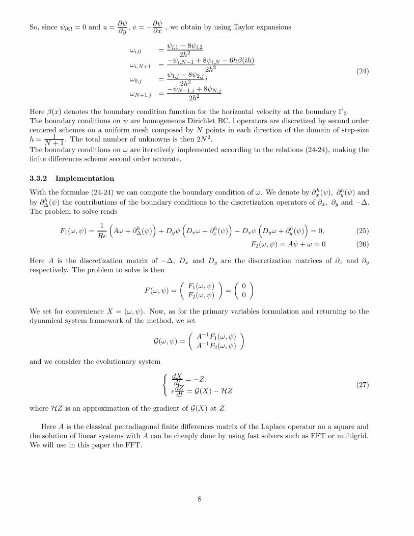
So, since ψ∂Ω = 0 and u =∂ψ∂y
, v = −∂ψ∂x
, we obtain by using Taylor expansions
ωi,0 =ψi,1 − 8ψi,2
2h2
ωi,N+1 =−ψi,N−1 + 8ψi,N − 6hβ(ih)
2h2
ω0,j =ψ1,j − 8ψ2,j
2h2 i
ωN+1,j =−ψN−1,j + 8ψN,j
2h2
(24)
Here β(x) denotes the boundary condition function for the horizontal velocity at the boundary Γ3.The boundary conditions on ψ are homogeneous Dirichlet BC. l operators are discretized by second ordercentered schemes on a uniform mesh composed by N points in each direction of the domain of step-sizeh = 1
N + 1. The total number of unknowns is then 2N 2.
The boundary conditions on ω are iteratively implemented according to the relations (24-24), making thefinite differences scheme second order accurate.
3.3.2 Implementation
With the formulae (24-24) we can compute the boundary condition of ω. We denote by ∂hx (ψ), ∂h
y (ψ) and
by ∂h∆(ψ) the contributions of the boundary conditions to the discretization operators of ∂x, ∂y and −∆.
The problem to solve reads
F1(ω, ψ) =1
Re
(
Aω + ∂h∆(ψ)
)
+Dyψ(
Dxω + ∂hx(ψ)
)
−Dxψ(
Dyω + ∂hy (ψ)
)
= 0, (25)
F2(ω, ψ) = Aψ + ω = 0 (26)
Here A is the discretization matrix of −∆, Dx and Dy are the discretization matrices of ∂x and ∂y
respectively. The problem to solve is then
F (ω, ψ) =
(
F1(ω, ψ)F2(ω, ψ)
)
=
(
00
)
We set for convenience X = (ω, ψ). Now, as for the primary variables formulation and returning to thedynamical system framework of the method, we set
G(ω, ψ) =
(
A−1F1(ω, ψ)A−1F2(ω, ψ)
)
and we consider the evolutionary system
dXdt = −Z,
εdZdt
= G(X) −HZ(27)
where HZ is an approximation of the gradient of G(X) at Z.
Here A is the classical pentadiagonal finite differences matrix of the Laplace operator on a square andthe solution of linear systems with A can be cheaply done by using fast solvers such as FFT or multigrid.We will use in this paper the FFT.
8
4 Numerical results
4.1 General implementation of the algorithm
We now list the information (data) required by the method:
• The number M .
• The parameters γ and ηk (that we will set to 0).
• The initial value of the descent parameter α0.
• The merit function. We use the Euclidian norm of the residual ‖F (X)‖.
• The accuracy of the global method: the solution is considered as accurate enough when ‖F (X)‖ <1.e− 6.
• The accuracy imposed for solving the preconditioning equation
F (xk + τz)− F (xk)
τ− F (xk) = 0,
that is characterized by
– the choice of the optimization method #1. We will use Enhanced Cauchy 2 as presented in theannex
– the number τ . We set τ = 1.e− 8
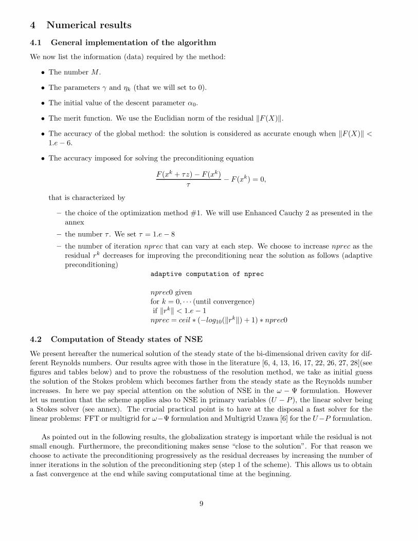
– the number of iteration nprec that can vary at each step. We choose to increase nprec as theresidual rk decreases for improving the preconditioning near the solution as follows (adaptivepreconditioning)
adaptive computation of nprec
nprec0 givenfor k = 0, · · · (until convergence)if ‖rk‖ < 1.e− 1nprec = ceil ∗ (−log10(‖r
k‖) + 1) ∗ nprec0
4.2 Computation of Steady states of NSE
We present hereafter the numerical solution of the steady state of the bi-dimensional driven cavity for dif-ferent Reynolds numbers. Our results agree with those in the literature [6, 4, 13, 16, 17, 22, 26, 27, 28](seefigures and tables below) and to prove the robustness of the resolution method, we take as initial guessthe solution of the Stokes problem which becomes farther from the steady state as the Reynolds numberincreases. In here we pay special attention on the solution of NSE in the ω − Ψ formulation. Howeverlet us mention that the scheme applies also to NSE in primary variables (U − P ), the linear solver beinga Stokes solver (see annex). The crucial practical point is to have at the disposal a fast solver for thelinear problems: FFT or multigrid for ω−Ψ formulation and Multigrid Uzawa [6] for the U−P formulation.
As pointed out in the following results, the globalization strategy is important while the residual is notsmall enough. Furthermore, the preconditioning makes sense “close to the solution”. For that reason wechoose to activate the preconditioning progressively as the residual decreases by increasing the number ofinner iterations in the solution of the preconditioning step (step 1 of the scheme). This allows us to obtaina fast convergence at the end while saving computational time at the beginning.
9
We observe that the number of outer iterations increases with the Reynolds number but not so muchwith the dimension of the problem. In all cases, the first part of the convergence process is devoted to“maintaining” the iterates in a neighborhood of the solution.All the computations have been made using Matlab c© software on a 2Ghz dual core PC with 2 ram’sGbytes.
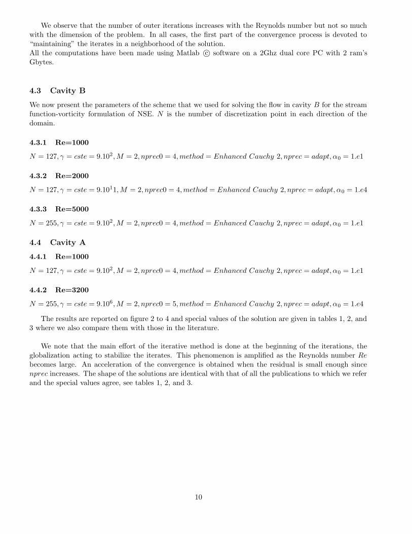
4.3 Cavity B
We now present the parameters of the scheme that we used for solving the flow in cavity B for the streamfunction-vorticity formulation of NSE. N is the number of discretization point in each direction of thedomain.
4.3.1 Re=1000
N = 127, γ = cste = 9.102,M = 2, nprec0 = 4,method = Enhanced Cauchy 2, nprec = adapt, α0 = 1.e1
4.3.2 Re=2000
N = 127, γ = cste = 9.1011,M = 2, nprec0 = 4,method = Enhanced Cauchy 2, nprec = adapt, α0 = 1.e4
4.3.3 Re=5000
N = 255, γ = cste = 9.102,M = 2, nprec0 = 4,method = Enhanced Cauchy 2, nprec = adapt, α0 = 1.e1
4.4 Cavity A
4.4.1 Re=1000
N = 127, γ = cste = 9.102,M = 2, nprec0 = 4,method = Enhanced Cauchy 2, nprec = adapt, α0 = 1.e1
4.4.2 Re=3200
N = 255, γ = cste = 9.106,M = 2, nprec0 = 5,method = Enhanced Cauchy 2, nprec = adapt, α0 = 1.e4
The results are reported on figure 2 to 4 and special values of the solution are given in tables 1, 2, and3 where we also compare them with those in the literature.
We note that the main effort of the iterative method is done at the beginning of the iterations, theglobalization acting to stabilize the iterates. This phenomenon is amplified as the Reynolds number Rebecomes large. An acceleration of the convergence is obtained when the residual is small enough sincenprec increases. The shape of the solutions are identical with that of all the publications to which we referand the special values agree, see tables 1, 2, and 3.
10

0 20 40 60 80 100 120 140 160 18010
−6
10−5
10−4
10−3
10−2
10−1
100
101
vorticite
x axes
y a
xes
0.1 0.2 0.3 0.4 0.5 0.6 0.7 0.8 0.9
0.1
0.2
0.3
0.4
0.5
0.6
0.7
0.8
0.9
x axes
y a
xes
0.1 0.2 0.3 0.4 0.5 0.6 0.7 0.8 0.9
0.1
0.2
0.3
0.4
0.5
0.6
0.7
0.8
0.9
0 0.2 0.4 0.6 0.8 1−0.4
−0.2
0
0.2
0.4
0.6
0.8
1median values of the vertical (*) and horizontal (+) velocity
U ,
V
x
Figure 2: Steady NSE, Re=1000, N=127. Residual vs iterations, median values of the horizontal and ofthe vertical velocity ; Isolines of the kinetic energy and of the vorticity
0.1 0.2 0.3 0.4 0.5 0.6 0.7 0.8 0.9
0.1
0.2
0.3
0.4
0.5
0.6
0.7
0.8
0.9
Figure 3: Steady NSE, Cavity B, Re=1000, N=127. Isolines of the stream function
11

0 100 200 300 400 500 60010
−6
10−5
10−4
10−3
10−2
10−1
100
101
vorticite
x axes
y a
xes
0.1 0.2 0.3 0.4 0.5 0.6 0.7 0.8 0.9
0.1
0.2
0.3
0.4
0.5
0.6
0.7
0.8
0.9
x axes
y a
xes
0.1 0.2 0.3 0.4 0.5 0.6 0.7 0.8 0.9
0.1
0.2
0.3
0.4
0.5
0.6
0.7
0.8
0.9
0 0.2 0.4 0.6 0.8 1−0.4
−0.2
0
0.2
0.4
0.6
0.8
1median values of the vertical (*) and horizontal (+) velocity
U ,
V
x
Figure 4: Steady NSE, Re=2000, N=127. Residual vs iterations, median values of the horizontal and ofthe vertical velocity ; Isolines of the kinetic energy and of the vorticity
0.1 0.2 0.3 0.4 0.5 0.6 0.7 0.8 0.9
0.1
0.2
0.3
0.4
0.5
0.6
0.7
0.8
0.9
Figure 5: Steady NSE, Cavity B, Re=2000, N=127 . Isolines of the stream function
12
0 200 400 600 800 1000 1200 140010
−6
10−5
10−4
10−3
10−2
10−1
100
101
vorticite
x axes
y a
xes
0.1 0.2 0.3 0.4 0.5 0.6 0.7 0.8 0.9
0.1
0.2
0.3
0.4
0.5
0.6
0.7
0.8
0.9
x axes
y a
xes
0.1 0.2 0.3 0.4 0.5 0.6 0.7 0.8 0.9
0.1
0.2
0.3
0.4
0.5
0.6
0.7
0.8
0.9
0 0.2 0.4 0.6 0.8 1−0.4
−0.2
0
0.2
0.4
0.6
0.8
1median values of the vertical (*) and horizontal (+) velocity
U ,
V
x
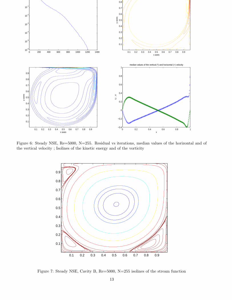
Figure 6: Steady NSE, Re=5000, N=255. Residual vs iterations, median values of the horizontal and ofthe vertical velocity ; Isolines of the kinetic energy and of the vorticity
0.1 0.2 0.3 0.4 0.5 0.6 0.7 0.8 0.9
0.1
0.2
0.3
0.4
0.5
0.6
0.7
0.8
0.9
Figure 7: Steady NSE, Cavity B, Re=5000, N=255 isolines of the stream function
13
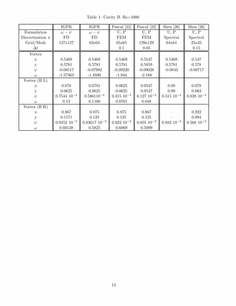
Table 1: Cavity B. Re=1000
IGPR IGPR Pascal [22] Pascal [22] Shen [26] Shen [26]
Formulation ω − ψ ω − ψ U, P U, P U, P U, PDiscretization x FD FD FEM FEM Spectral Spectral
Grid/Mesh 127x127 63x63 65x65 129x129 64x64 25x25∆t 0.1 0.05 0.15
Vortexx 0.5469 0.5469 0.5469 0.5547 0.5469 0.547y 0.5781 0.5781 0.5781 0.5859 0.5781 0.578ψ -0.08517 -0.07982 -0.09220 -0.09028 -0.0843 -0.08717ω -1.57363 -1.4930 -1.944 -2.168
Vortex (B L)x 0.078 0.0781 0.0625 0.0547 0.08 0.078y 0.0625 0.0625 0.0625 0.0547 0.09 0.063ψ 0.7544 10−4 0.586110−4 0.315 10−4 0.127 10−4 0.515 10−4 0.828 10−4
ω 0.13 0.1160 0.0761 0.048
Vortex (B R)x 0.867 0.875 0.875 0.867 – 0.922y 0.1171 0.125 0.125 0.125 – 0.094ψ 0.9452 10−3 0.83617 10−3 0.922 10−3 0.855 10−3 0.882 10−3 0.568 10−3
ω 0.60138 0.5825 0.6069 0.5099
14

Table 2: Cavity B. Re=2000
IGPR Shen [26] Shen [26]
Formulation ω − ψ ω − ψ ω − ψDiscretization x FD Spectral Spectral
Grid / Mesh 127x127 33x33 25x25∆t
Vortexx 0.5312 0.516 0.531y 0.5546 0.547 0.547ψ -0.08361 -0.08776 -0.08762ω -1.4370
Vortex (B L)x 0.08593 0.094 0.078y 0.09375 0.094 0.094ψ 3.1435 10−4 3.5432 10−4 3.1772 10−4
ω 0.3862
Vortex (B R)x 0.8515 0.922 0.922y 0.1015 0.094 0.094ψ 1.495 10−3 0.80841 10−3 0.80667 10−3
ω 0.9448
Vortex (U L)x 0.03125 0.031 0.031y 0.8906 0.92 0.92ψ 5.1499 10−5 1.449710−5 1.714310−5
ω 0.3051
15

Table 3: Cavity B. Re=5000
IGPR IGPR Shen [27] Pascal [22]
Formulation ω − ψ ω − ψ U, P U, PDiscretization x FD FD Spectral FEM
Grid / Mesh 127x127 255x255 33x33 129x129∆t 0.03 0.05
Vortexx 0.5234 0.51953 0.516 0.5390y 0.539 0.539 0.531 0.5313ψ -0.07761 -0.085211 -0.08776 -0.0975ω -1.2687 -1.3866 -2.169
Vortex (B L)x 0.078125 0.78125 0.094 0.0859y 0.125 0.125 0.094 0.1172ψ 6.8393 10−4 7.9510−4 7.5268 10−4 6.72310−4
ω 0.7468 0.844 0.7310
Vortex (B R)x 0.8203 0.8164 0.922 0.8047y 0.08593 0.082 0.094 0.0781ψ 1.8528 10−3 2.04110−3 0.77475 10−3 2.42 10−3
ω 1.42177 1.58687 2.009
Vortex (U L)x 0.07812 0.0859 0.078 0.0781y 0.9062 0.9101 0.92 0.906ψ 5.6645 10−4 7.14910−4 6.77810−4 7.86 10−4
ω 0.88813 1.098 1.159
16

0 50 100 150 200 25010
−6
10−5
10−4
10−3
10−2
10−1
100
101
vorticite
x axes
y a
xes
0.1 0.2 0.3 0.4 0.5 0.6 0.7 0.8 0.9
0.1
0.2
0.3
0.4
0.5
0.6
0.7
0.8
0.9
x axes
y a
xes
0.1 0.2 0.3 0.4 0.5 0.6 0.7 0.8 0.9
0.1
0.2
0.3
0.4
0.5
0.6
0.7
0.8
0.9
0 0.2 0.4 0.6 0.8 1−0.6
−0.4
−0.2
0
0.2
0.4
0.6
0.8
1median values of the vertical (*) and horizontal (+) velocity
U ,
V
x
Figure 8: Steady NSE, Re=1000, N=127. Residual vs iterations, median values of the horizontal and ofthe vertical velocity ; Isolines of the kinetic energy and of the vorticity
0.1 0.2 0.3 0.4 0.5 0.6 0.7 0.8 0.9
0.1
0.2
0.3
0.4
0.5
0.6
0.7
0.8
0.9
Figure 9: Steady NSE, Cavity A, Re=1000, N=127. Isolines of the stream function
17
0 200 400 600 800 100010
−6
10−5
10−4
10−3
10−2
10−1
100
101
vorticite
x axes
y a
xes
0.1 0.2 0.3 0.4 0.5 0.6 0.7 0.8 0.9
0.1
0.2
0.3
0.4
0.5
0.6
0.7
0.8
0.9
x axes
y a
xes
0.1 0.2 0.3 0.4 0.5 0.6 0.7 0.8 0.9
0.1
0.2
0.3
0.4
0.5
0.6
0.7
0.8
0.9
0 0.2 0.4 0.6 0.8 1−0.6
−0.4
−0.2
0
0.2
0.4
0.6
0.8
1median values of the vertical (*) and horizontal (+) velocity
U ,
V
x
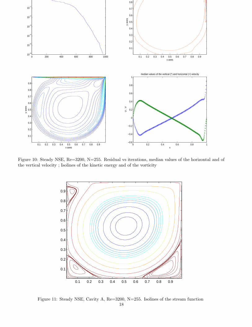
Figure 10: Steady NSE, Re=3200, N=255. Residual vs iterations, median values of the horizontal and ofthe vertical velocity ; Isolines of the kinetic energy and of the vorticity
0.1 0.2 0.3 0.4 0.5 0.6 0.7 0.8 0.9
0.1
0.2
0.3
0.4
0.5
0.6
0.7
0.8
0.9
Figure 11: Steady NSE, Cavity A, Re=3200, N=255. Isolines of the stream function18
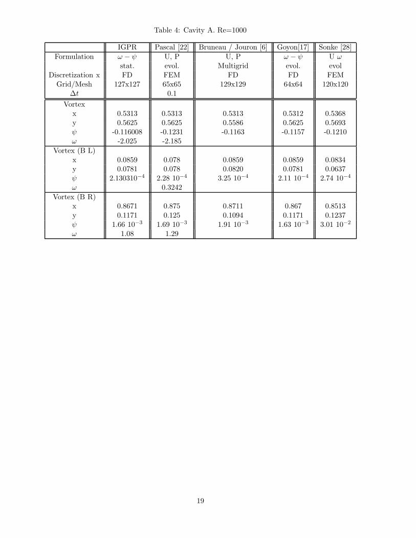
Table 4: Cavity A. Re=1000
IGPR Pascal [22] Bruneau / Jouron [6] Goyon[17] Sonke [28]
Formulation ω − ψ U, P U, P ω − ψ U ωstat. evol. Multigrid evol. evol
Discretization x FD FEM FD FD FEMGrid/Mesh 127x127 65x65 129x129 64x64 120x120
∆t 0.1
Vortexx 0.5313 0.5313 0.5313 0.5312 0.5368y 0.5625 0.5625 0.5586 0.5625 0.5693ψ -0.116008 -0.1231 -0.1163 -0.1157 -0.1210ω -2.025 -2.185
Vortex (B L)x 0.0859 0.078 0.0859 0.0859 0.0834y 0.0781 0.078 0.0820 0.0781 0.0637ψ 2.130310−4 2.28 10−4 3.25 10−4 2.11 10−4 2.74 10−4
ω 0.3242
Vortex (B R)x 0.8671 0.875 0.8711 0.867 0.8513y 0.1171 0.125 0.1094 0.1171 0.1237ψ 1.66 10−3 1.69 10−3 1.91 10−3 1.63 10−3 3.01 10−2
ω 1.08 1.29
19
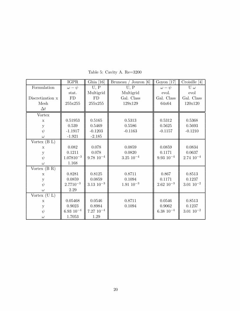
Table 5: Cavity A. Re=3200
IGPR Ghia [16] Bruneau / Jouron [6] Goyon [17] Croisille [4]
Formulation ω − ψ U, P U, P ω − ψ U ωstat. Multigrid Multigrid evol. evol
Discretization x FD FD Gal. Class Gal. Class Gal. ClassMesh 255x255 255x255 129x129 64x64 120x120∆t
Vortexx 0.51953 0.5165 0.5313 0.5312 0.5368y 0.539 0.5469 0.5586 0.5625 0.5693ψ -1.1917 -0.1203 -0.1163 -0.1157 -0.1210ω -1.921 -2.185
Vortex (B L)x 0.082 0.078 0.0859 0.0859 0.0834y 0.1211 0.078 0.0820 0.1171 0.0637ψ 1.07810−3 9.78 10−4 3.25 10−4 9.93 10−4 2.74 10−4
ω 1.168
Vortex (B R)x 0.8281 0.8125 0.8711 0.867 0.8513y 0.0859 0.0859 0.1094 0.1171 0.1237ψ 2.7710−3 3.13 10−3 1.91 10−3 2.62 10−3 3.01 10−2
ω 2.29
Vortex (U L)x 0.05468 0.0546 0.8711 0.0546 0.8513y 0.9023 0.8984 0.1094 0.9062 0.1237ψ 6.93 10−4 7.27 10−4 6.38 10−4 3.01 10−2
ω 1.7053 1.29
20

5 Concluding remarks
We have presented a scheme that takes into account only the linear part of the equation for solving steadyfluid flows, making our method a very general one. The efficiency of the scheme is increased when a fastsolver is used for the linear problem. The results we obtain on the numerical solution of NSE show thatthe proposed method is robust; as it has been already established, it is harder to solve directly the steadyNSE than to compute the steady state by time marching schemes applied to the evolutionary equation.The new method is also flexible since the choice of the preconditioning step is completely free. We wouldlike to stress out that the preconditioned globalized spectral gradient method can be applied in a largenumber of situation and fields, especially when no (simple) preconditioning can be built, such as in CFD,and also in numerical linear algebra when solving Riccati matrix equations or for some other nonlinearmatrix problems. This is a topic that deserves further investigation.
Acknowledgements This work was supported by SIMPAF project from INRIA futurs.
References
[1] J. Barzilai and J. M. Borwein (1988). Two-point step size gradient methods, IMA Journal of Numerical
Analysis, 8, 141–148.
[2] P. Brown, and Y. Saad (1990). Hybrid Krylov methods for nonlinear systems of equations, SIAM
Journal on Scientific Computing 11, 450–481.
[3] P. Brown, and Y. Saad (1994). Convergence theory of nonlinear Newton-Krylov algorithms, SIAM
Journal on Optimization 4, 297–330.
[4] M. Ben-Artzi, J.-P. Croisille, D. Fishelov and S. Trachtenberg (2005). A pure-compact scheme forthe streamfunction formulation of Navier-Stokes equations, Journal Comp. Phys., 205 (2005), no 2,640–664.
[5] C. Brezinski, J.-P. Chehab, Nonlinear hybrid procedures and fixed point iterations, Num. Func. Anal.Opt., 19 (1998), 465-487.
[6] C.-H. Bruneau and C. Jouron (1990). An efficient Scheme for solving Steady incompressible Navier-STokes equations, Journal Comp. Phys. 89, 389–413.
[7] A. Cauchy [1847], Methodes generales pour la resolution des systemes d’equations simultanees, C. R.
Acad. Sci. Par. 25, pp. 536–538.
[8] J.-P. Chehab and J. Laminie, Differential equations and solution of linear systems, Numerical Algo-rithms (2005), 40, 103-124.
[9] J.-P. Chehab and M. Raydan (2005). Inverse and adaptive preconditioned gradient methods for non-linear problems, Num. Math. 55, 32–47
[10] M. Crouzeix, Approximation et methodes iteratives de resolution d’inequations variationelles et de
problemes non lineaires, I.R.I.A., cahier 12, Mai 1974, 139-244.
[11] Y. H. Dai and L. Z. Liao (2002). R-linear convergence of the Barzilai and Borwein gradient method,IMA Journal on Numerical Analysis 22, pp. 1–10.
[12] J.E. Dennis Jr. and R.B. Schnabel (1983), Numerical Methods for Unconstrained Optimization and
Nonlinear Equations, Prentice-Hall, Englewood Cliffs, NJ.
21
[13] E. Erturk, T.C. Corke and C. Gokcol, Numerical Solutions of 2-D Steady Incompressible DrivenCavity Flow at High Reynolds Numbers, Int. J. Numer. Meth. Fluids 2005, Vol 48, pp 747-774.
[14] D. Euvrard, Resolution numerique des equations aux derivees partielles, Dunod, 350 pp, 1994, 3rdEdition.
[15] R. Fletcher (2005). On the Barzilai-Borwein method. In: Optimization and Control with Applications
(L.Qi, K. L. Teo, X. Q. Yang, eds.) Springer, 235–256.
[16] U. Ghia, K.N. Ghia and C.T. Shin (1982). High-Re Solutions of incompressible Flow using the Navier-Stokes equations and the multigrid method, Journal Comp. Phys. 48, 387–411.
[17] O. Goyon (1996). High-Reynolds Number Solutions of Navier-Stokes Equations using IncrementalUnknowns, Comput. Meth. Appl. Mech. and Eng. 130, 319–335.
[18] C. T. Kelley (1995). Iterative Methods for Linear and Nonlinear Equations. SIAM, Philadelphia.
[19] W. La Cruz and M. Raydan (2003). Nonmonotone Spectral Methods for Large-Scale Nonlinear Sys-tems, Optimization Methods and Software, 18, 583–599.
[20] W. La Cruz, J. M. Martınez and M. Raydan (2004). Spectral residual method without gradientinformation for solving large-scale nonlinear systems, Math. of Comp., to appear.
[21] F. Luengo, M. Raydan, W. Glunt, T.L. Hayden, Preconditioned spectral gradient method, Numerical
Algorithms, Vol. 30, pp. 241-258, 2002.
[22] F. Pascal, Methodes de Galerkin non linaires en discretisation par elements finis et pseudo-spectrale.
Application a la mecanique des fluides, These Universite Paris XI, Orsay, janvier 1992.
[23] R. Peyret, R. Taylor, Computational methods for fluid flows, Springer series in Computational Physics,Springer 1983.
[24] M. Raydan (1993). On the Barzilai and Borwein choice of the steplength for the gradient method,IMA Journal on Numerical Analysis 13, 321–326.
[25] M. Raydan (1997). The Barzilai and Borwein gradient method for the large scale unconstrainedminimization problem, SIAM Journal on Optimization, 7, 26–33.
[26] J. Shen (1990). Numerical simulation of the regularized driven cavity flows at high Reynolds numbers,Comput. Meth. in Applied Mech. and Eng. 80, 273–280.
[27] J. Shen (1991). Hopf bifurcation of the Unsteady regularized driven cavity flow, J. Comput. Phys. 95,228–245.
[28] L. Sonke Tabuguia, Etude numerique des equations des Navier-Stokes en milieux multiplement con-
nexes, en formulation vitesse-tourbillon, par une approche multidomaine Paris XI, Orsay, 1989.
[29] R. Temam, Navier Stokes equations, North Holland, 1984.
[30] S. Turek, Efficient dsolvers for incompressible flows problems, Lecture Notes in Computational Scienceand Engineering, Springer, 1999.
[31] L.B. Zhang, Un schema de semi-discretisation en temps pour des systemes differentiels discretises en
espace par la methode de Fourier. Resolution numerique des equations de Navier-Stokes stationnaires
par la methode multigrille. These, Universite Paris–Sud, Orsay, 1987.
22
6 Annex
6.1 Solution of NSE in primary variables
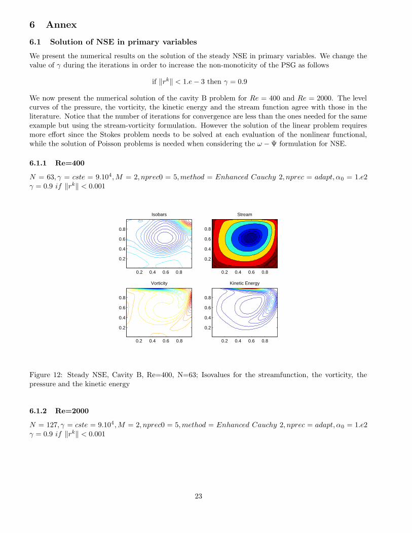
We present the numerical results on the solution of the steady NSE in primary variables. We change thevalue of γ during the iterations in order to increase the non-monoticity of the PSG as follows
if ‖rk‖ < 1.e− 3 then γ = 0.9
We now present the numerical solution of the cavity B problem for Re = 400 and Re = 2000. The levelcurves of the pressure, the vorticity, the kinetic energy and the stream function agree with those in theliterature. Notice that the number of iterations for convergence are less than the ones needed for the sameexample but using the stream-vorticity formulation. However the solution of the linear problem requiresmore effort since the Stokes problem needs to be solved at each evaluation of the nonlinear functional,while the solution of Poisson problems is needed when considering the ω −Ψ formulation for NSE.
6.1.1 Re=400
N = 63, γ = cste = 9.104,M = 2, nprec0 = 5,method = Enhanced Cauchy 2, nprec = adapt, α0 = 1.e2γ = 0.9 if ‖rk‖ < 0.001
Isobars
0.2 0.4 0.6 0.8
0.2
0.4
0.6
0.8
Stream
0.2 0.4 0.6 0.8
0.2
0.4
0.6
0.8
Vorticity
0.2 0.4 0.6 0.8
0.2
0.4
0.6
0.8
Kinetic Energy
0.2 0.4 0.6 0.8
0.2
0.4
0.6
0.8
Figure 12: Steady NSE, Cavity B, Re=400, N=63; Isovalues for the streamfunction, the vorticity, thepressure and the kinetic energy
6.1.2 Re=2000
N = 127, γ = cste = 9.104,M = 2, nprec0 = 5,method = Enhanced Cauchy 2, nprec = adapt, α0 = 1.e2γ = 0.9 if ‖rk‖ < 0.001
23
0 5 10 15 20 2510
−8
10−6
10−4
10−2
100
102
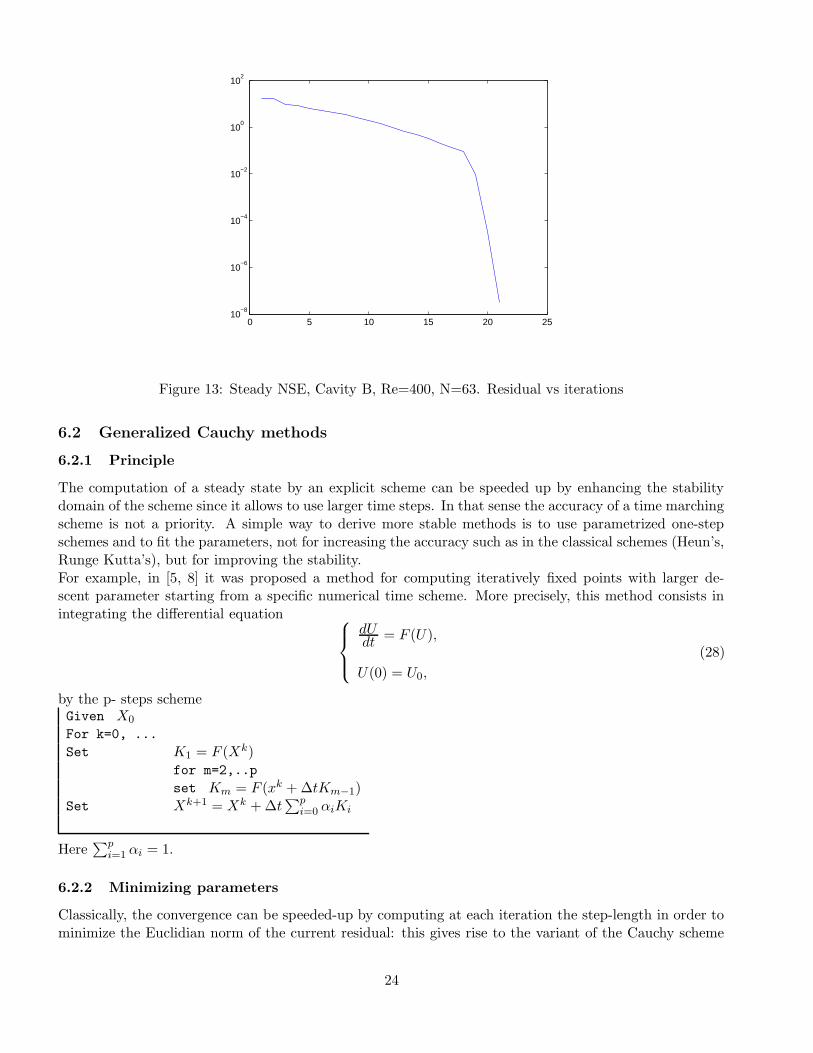
Figure 13: Steady NSE, Cavity B, Re=400, N=63. Residual vs iterations
6.2 Generalized Cauchy methods
6.2.1 Principle
The computation of a steady state by an explicit scheme can be speeded up by enhancing the stabilitydomain of the scheme since it allows to use larger time steps. In that sense the accuracy of a time marchingscheme is not a priority. A simple way to derive more stable methods is to use parametrized one-stepschemes and to fit the parameters, not for increasing the accuracy such as in the classical schemes (Heun’s,Runge Kutta’s), but for improving the stability.For example, in [5, 8] it was proposed a method for computing iteratively fixed points with larger de-scent parameter starting from a specific numerical time scheme. More precisely, this method consists inintegrating the differential equation
dUdt
= F (U),
U(0) = U0,
(28)
by the p- steps schemeGiven X0
For k=0, ...
Set K1 = F (Xk)for m=2,..p
set Km = F (xk + ∆tKm−1)Set Xk+1 = Xk + ∆t
∑pi=0 αiKi
Here∑p
i=1 αi = 1.
6.2.2 Minimizing parameters
Classically, the convergence can be speeded-up by computing at each iteration the step-length in order tominimize the Euclidian norm of the current residual: this gives rise to the variant of the Cauchy scheme
24

0.2 0.4 0.6 0.8
0.2
0.4
0.6
0.8
Isobars
0.2 0.4 0.6 0.8
0.2
0.4
0.6
0.8
Stream
0.2 0.4 0.6 0.8
0.2
0.4
0.6
0.8
Vorticity
0.2 0.4 0.6 0.8
0.2
0.4
0.6
0.8
Kinetic Energy
Figure 14: Steady NSE, Cavity B, Re=2000, N=127; Isovalues for the stream function, the vorticity, thepressure and the kinetic energy
[7]. Of course the minimizing parameter becomes harder to compute as p increases. We list hereafter theoptimal values of the parameters for p = 1, 2, 3
• p = 1 (Cauchy method)
αki = 1,∆tk =
< Ark, rk >
‖Ark‖2
• p = 2 (Enhanced Cauchy 1 (EC1) see [8, 9])We set
a = ‖rk‖2, b =< Ark, rk >, c = ‖Ark‖2, d =< A2rk, rk >, e =< A2rk, Ark >, f =< A2rk, A2rk >,
∆tk =fb− ed
fc− e2, α1 = 1−
∆tke− d
∆t2kf, α2 = 1− α1
• p = 3 (Enhanced Cauchy 2 (EC2))We set
a = ‖Ark‖2, b = ‖A2rk‖2, c = ‖A3rk‖2, d =< Ark, rk >, e =< A2rk, rk >,f =< A3rk, rk >, g =< A2rk, Ark >, hh =< A3rk, Ark >, ii =< A3rk, A2rk >
∆tk =−hh ii e− g ii f + hh f b+ d ii2 − d c b+ g c e
(g2 c+ hh2 b− a c b+ a ii2 − 2 hh ii g)
α1 =(ii f − ii ∆tk hh+ (∆tk)
2 ii2 − (∆tk)2 b c− e c+ ∆tk g c)
((∆tk)2 (−b c+ ii2))
α2 = −(∆tk ii f − hh (∆tk)
2 ii− dt e c+ (∆tk)2 g c− f b+ ∆tk hh b+ ii e− ii ∆tk g)
((∆tk)3 (−b c+ ii2))
α3 = 1− α1 − α2
25
0 10 20 30 40 50 60 70 8010
−6
10−5
10−4
10−3
10−2
10−1
100
101
102
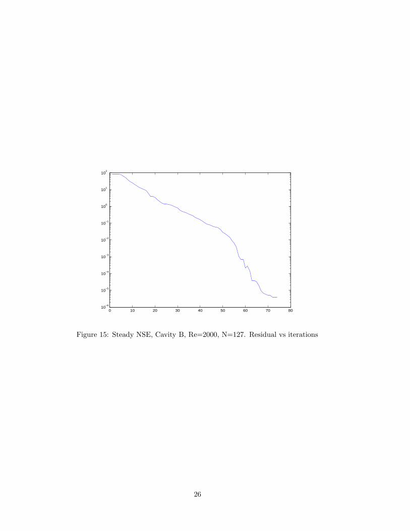
Figure 15: Steady NSE, Cavity B, Re=2000, N=127. Residual vs iterations
26