A Simple Introduction to Embedded Control Systems …s-iihr64.iihr.uiowa.edu/MyWeb/Teaching/ECE3360_2016/Lectures/PID... · A Simple Introduction to Embedded Control ... –F. Vahid

Slide 1 Embedded Systems and Software, ECE:3360. The University of Iowa, 2016 A. Kruger

Embedded Systems and Software

A Simple Introduction to Embedded Control

Systems (PID Control)


Acknowledgements

• The material in this lecture is adapted from:

– F. Vahid and T. Givargis, Embedded System Design—A Unified

Hardware/Software Introduction, John Wiley & Sons, 2002

(Chapter 9)

– T. Wescott, “PID Without a PhD”

http://www.embedded.com/2000/0010/0010feat3.htm


Control System Terminology

• Control physical system (plant) output

– By setting plant’ input

• Examples

– Cruise control, thermostat, disk drive, chemical processes

• Difficulty due to

– Disturbance: wind, road, tire, brake; opening/closing door…

– Human interface: feel good, feel right…


Control System Tracking

Reference Input a.k.a. Set Point

where we want the output to be

For example, here the user turned

up the thermostat

This how the system tracks the

reference input or set point


Control System Tracking

Reference Input a.k.a. Set Point

where we want the output to be

For example, here the user turned

up the thermostat

This how the system tracks the

reference input or set point


• Plant

– Physical system to be controlled: car, plane, disk, heater,…

• Actuator

– Device to control the plant: throttle, wing flap, disk motor,…

• Controller

– Designed product to control the plant

Open-Loop Control Systems


• Output (𝒗𝒕)

– What we are interested in: speed, disk location, temperature

• Reference Input / Set Point (𝒓𝒕)

– Desired output: speed, desired location, desired temperature

• Disturbance (𝒘𝒕)

– Uncontrollable input to the plant imposed by environment

Wind, bumping the disk drive, door opening

Open-Loop Control Systems

7


• Feed-forward control

• Delay in actual change of the output

• Controller doesn’t know how well things are going

• Simple

• Best use for predictable systems

– Examples?

Characteristics of Open Loop Control


Closed Loop Control System

Control Law: 𝑢𝑡 = 𝐹 𝑒𝑡

Plant Model

System Model

𝑣𝑡+1 = 𝐹(𝑣𝑡 , 𝑢𝑡 , 𝑤𝑡)

𝑣𝑡+1 = 𝐹(𝑣𝑡 , 𝑢𝑡 , 𝑤𝑡) Goal: minimize tracking error 𝑒𝑡

Σ −

+

Sensor

Controller Plant

Plant Model Set Point (𝑟𝑡)

Disturbance (𝑤𝑡) Error (𝑒𝑡 = 𝑟𝑡 − 𝑣𝑡)

𝑢𝑡 = 𝐹 𝑒𝑡 𝑣𝑡 𝑢𝑡


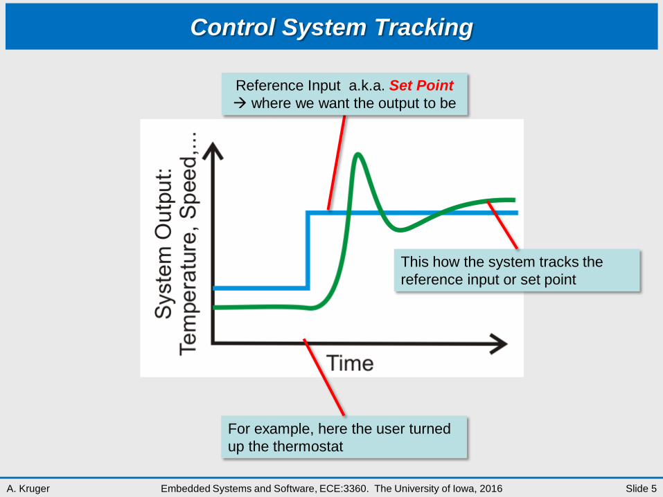
Example Closed Loop Control System

ttt vrPu tttt wu.vv 507.01

ttt

ttttt

wPr.vP..

wvrPvv

505070

)(5.07.01

Plant Model

System Model

Control Law

Σ −

+

Sensor

Controller Plant





Model of the Plant

Counter-intuitively, it may not necessary to (accurately) model the plant

Σ −

+

Sensor

Controller Plant




However, even a simple model can be very helpful


Model the car speed at 𝑡 + 1 as a linear combination of

the speed at t (i.e., 𝑣𝑡) and the throttle at 𝑡 (i.e., 𝑢𝑡) vt+1 = Avt + But

Next, experimentally determine the model parameters A and B. On flat surface at 50 mph,

open the throttle to 40 degrees. Then measure the speed after one time unit. Assume the

speed is 55 mph. Then

55 = 50A + 40B

Repeat the experiment, but now start at 65 mph and with the throttle at 50 degrees.

Assume the resulting speed after one time unit is 70.5 mph. Then

70.5 = 65A + 50B

One can now solve these two equations for the two unknowns 𝐴 and 𝐵, to find 𝐴 = 0.7 and 𝐵 = 0.5.

One can repeat the experiment many times and determine, say, average values for 𝐴 and

𝐵. (There are more optimum techniques for dealing with multiple 𝐴s and 𝐵s). Regardless,

we now have model for the car (plant).

vt+1 = 0.7vt + 0.5ut

Example


Closed-Loop Control

BABBAvABBABvAABvAv 2

0

3

0

2

23

ttt

ttttt

wPr.vP..

wvrPvv

505070

)(5.07.01

ttt vrPu tttt wu.vv 507.01

BvAv tt 1

005.0,5.07.0 wPrBPA

BvAv 01

BABvABBvAABvAv 0

2

012

BAAvAv nnn

n 121

0

Consider fixed set point and fixed disturbance

001 505070 wPr.vP..v tt

00

21

0 5.015.07.05.07.05.07.0 wPrPPvPvnnn

n

Plant model Control Law (feedback)


Tuning Performance: Finding Proper P

00

21

0 5.015.07.05.07.05.07.0 wPrPPvPvnnn

n

To obtain convergence requires 15.07.0 P 4.36.0 P

To avoid oscillation requires 05.07.0 P 4.1 P

Reduce the effect of initial conditions (v0), make (0.7-0.5P) as small as possible 4.1 P

001 505070 wPr.vP..v tt 450 tt vrPu

Σ −

+

Sensor

Controller Plant



𝑢𝑡 = −𝑃 𝑒𝑡 𝑣𝑡 𝑢𝑡


Steady state means vss = vt + 1 = vt 00505070 wPr.vP..v ssss

P

wr

P

Pvss

5.03.05.03.0

5.0 00

To get vss as close as possible to r0, (perfect tracking) let P ∞

00

21

0 5.015.07.05.07.05.07.0 wPrPPvPvnnn

n

001 505070 wPr.vP..v tt 450 tt vrPu

Σ −

+

Sensor

Controller Plant





Tuning Performance: Finding Proper P

To obtain convergence requires 15.07.0 P 4.36.0 P

To avoid oscillation requires 05.07.0 P 4.1 P

Reduce the effect of initial conditions (v0), make (0.7-0.5P) as small as possible 4.1 P

To get vss as close as possible to r0, (perfect tracking) let P ∞

Finally, pick 3.3P stable, fast, good tracking, but some oscillation

Σ −

+

Sensor

Controller Plant





0 10 20 30 40 50 600

10

20

30

40

50

60

70

Control Point (i.e., time)

Sp

ee

d (

mp

h)

Analyze Controller Performance

0 mph,50 mph,20 00 wrv t

01 505070 Pr.vP..v tt

01 )3.3(50)3.3(5070 r.v..v tt

5.8295.01 tt vv

tt vrPu 0 tt vu 503.3

Valid range for controller is 0-45o. Thus, with

this P, the actuator saturates.

Tracking error ~ 8 mph

Significant oscillation

3.3P


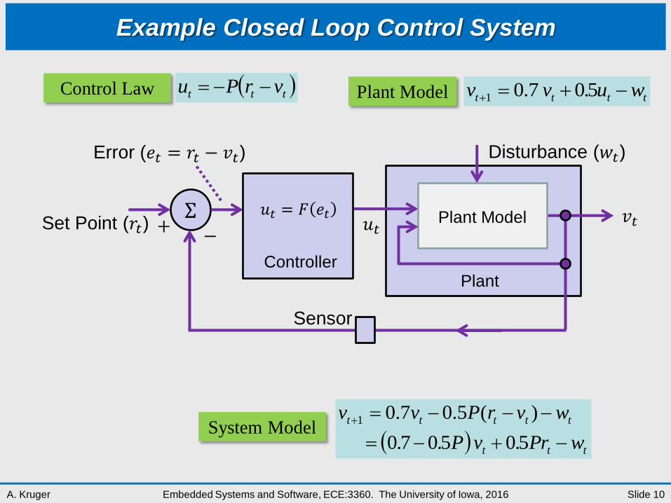
Analyze Controller Performance

0 10 20 30 40 50 600

10

20

30

40

50

60

70


Sp

ee

d (

mp

h)

Tracking error ~ 20 mph

No oscillation

Valid range for controller is 0-45o. Thus, with

this P=1, the actuator does not saturate.

Set P = 1 to avoid oscillation


Analyzing the Controller

0 10 20 30 40 50 600

10

20

30

40

50

60

70


Sp

ee

d (

mp

h)

P = 1.0

P = 3.3 P = 2.5

Set point (where we want to be)


Closed-Loop Performance

0 10 20 30 40 50 600

10

20

30

40

50

60

70


Sp

ee

d (

mp

h)

P = 3.3, W =+5 P = 3.3, W =0

P = 3.3, W = - 5

0 mph,50 mph,20 000 wrv

01 505070 Pr.vP..v tt

01 )3.3(50)3.3(5070 r.v..v tt

01 5.8295.0 wvv tt

Change is 5 mph compared to 66-

33 = 33 mph for open-loop control


• Objective

– Causing output to track a reference even in the presence of

Measurement noise

Model error

Disturbances

• Metrics

– Stability

Output remains bounded

– Performance

How well an output tracks the reference

– Disturbance rejection

– Robustness

Ability to tolerate modeling error of the plant

General Control System


Performance (generally speaking)

• Rise time – Time it takes

from 10% to 90%

• Peak time

• Overshoot – Percentage by

which Peak exceed final value

• Settling time – Time it takes to

reach 1% of final value


• Difficult

• May need to be done first

• Plant is usually on continuous time

– Not discrete time. For example, car speed continuously reacts to

throttle position, not at discrete interval

– Sampling period must be chosen carefully to ensure “nothing

interesting” happens in between sampling intervals

• Plant is usually non-linear

– For example, shock absorber response may need to be 8th order

differential equation

• Iterative development of the plant model and controller

– Have a plant model that is “good enough”

Plant Modeling


Controller Design: “P”

tt vrPu 0Proportional control - multiplies the tracking error with a constant P

P affects

Stability

Tracking

Disturbance rejection

Large P can lead to overshoot and oscillation

Make P large to reduce tracking error

Make P large to improve disturbance rejection

001 505070 wPr.vP..v tt Closed-loop model with linear plant

Σ −

+

Sensor

Controller Plant





Controller Design: “PD”

Proportional and Derivative control - P control, and also consider error over time

Intuitively

Want to “push” more if error is not reducing fast enough

Want to “push” less if error is reducing really fast

11 ttttttt vrvrDvrPu

1 tttt eeDPeu


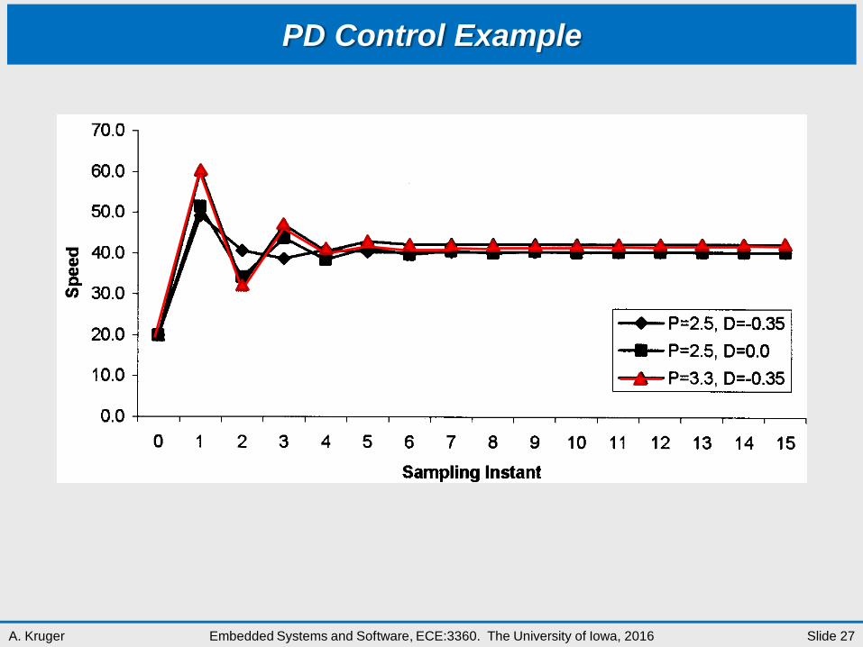
PD Controller

1 tttt eeDPeu

tttt wu.vv 507.01 Plant model

Control Law (feedback)

ttttttttt wvrvrDvrP.vv 111 507.0

ttt vre

ttttttt wDrrDPDvvDP.vv 111 5.05.05.0507.0

05.07.01

5.0r

P

Pvss

Assume reference input and disturbance are constant, then the steady-state speed is

P can be set for best tracking and disturbance control

Then D can be set to control transient behavior

Does not depend on D

Steady state means vss = vt + 1 = vt


PD Control Example


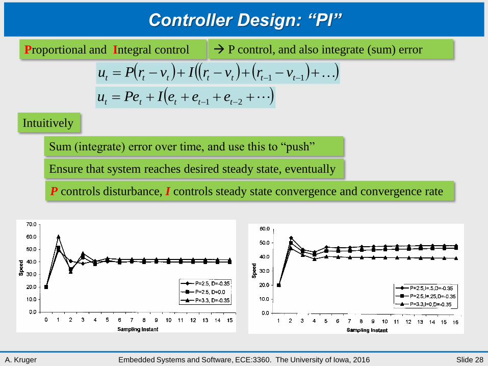
Controller Design: “PI”

Proportional and Integral control P control, and also integrate (sum) error

Intuitively

Sum (integrate) error over time, and use this to “push”

Ensure that system reaches desired steady state, eventually

11 ttttttt vrvrIvrPu

21 ttttt eeeIPeu

P controls disturbance, I controls steady state convergence and convergence rate


Controller Design: “PID”

Proportional , Integral and Derivative control - use all 3 types of control

Intuitively

P considers current error, controls disturbance

I controls long-term error, controls steady state convergence and convergence rate

1111 ttttttttttt vrvrDvrvrIvrPu

121 ttttttt eeDeeeIPeu

D considers how error is changing, controls transient response


Examples


• More than 90% of all controllers

used in process industries are PID

controllers.

• A typical chemical plant has 100s

or more PID controllers.

• PID controllers are widely used in:

– Chemical plants

– Oil refineries

– Pharmaceutical industries

– Food industries

– Paper mills

– Electronic equipments

Application of PID Control

http://upload.wikimedia.org/wikipedia/commons/a/a2/Harddisk-full.jpg


Off-The-Shelf PID Controllers

There are many off-the-shelf PID controllers available


Block Diagram View of PID Controller


Another Block Diagram View of PID Controller

Set desired input



Compare actual output against set point



Use part of the error signal



Use sum of the previous errors



Use rate of change of errors



Update the process, and repeat


Sidebar: Analog PID Controller

Integral

Proportional

Derivative

Summer


PID Pseudo Code

previous_error = 0

integral = 0

start:

get actual_position

error = setpoint - actual_position

integral = integral + error*dt

derivative = (error - previous_error)/dt

output = P*error + I*integral + D*derivative

previous_error = error

wait(dt)

goto start


• Main function loops forever, during each iteration

– Read plant output sensor (may require ADC)

– Read current desired reference input (set point)

– Call a routine PidUpdate, to determine actuator value

– Set actuator value (may require DAC)

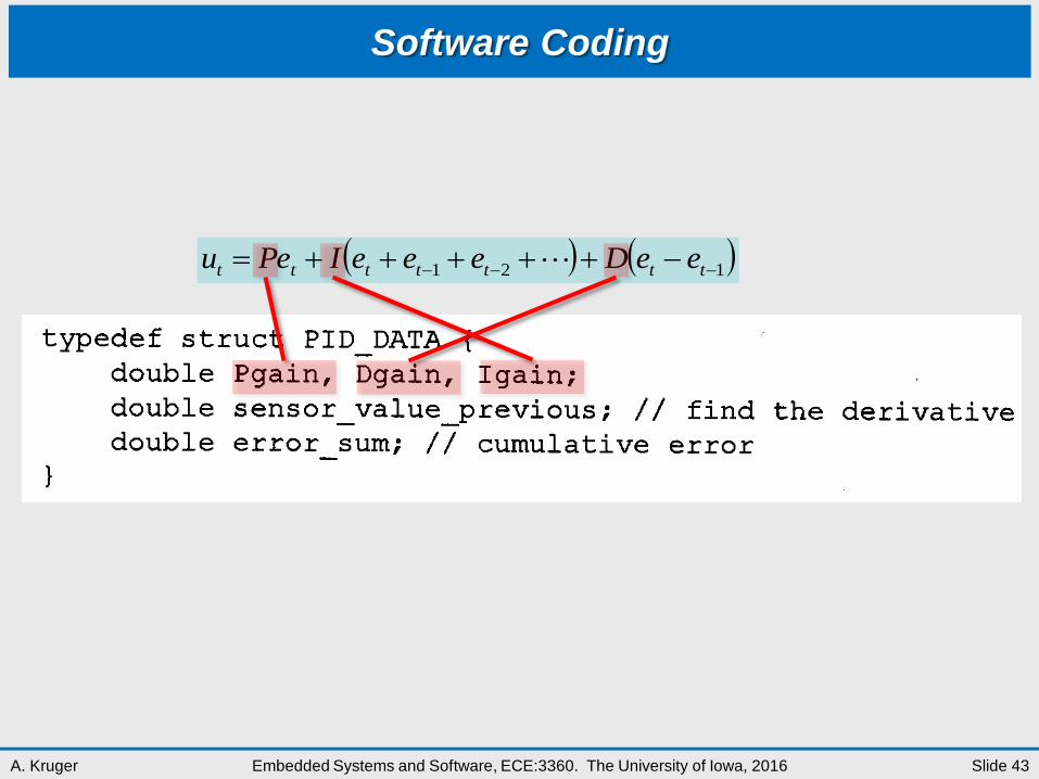
Software Coding


Software Coding



Computation



• Analytically deriving P, I, D may not be possible

– E.g., plant not is not available, or to costly to obtain

• Ad hoc method for getting “reasonable” P, I, D

– Start with a small P, I = D = 0

– Increase D, until seeing oscillation, then reduce D a bit

– Increase P, until seeing oscillation, then D a bit

– Increase I, until seeing oscillation

• Iterate until one can change anything without excessive

oscillation

PID Tuning


• Quantization

• Overflow

• Aliasing

• Computation Delay

Practical Issues with Computer-Based Control


Quantization & Overflow

• Quantization – E.g., can’t store 0.36 as 4-bit fractional number

– Can only store 0.75, 0.59, 0.25, 0.00, -0.25, -050,-0.75, -1.00

– Choose 0.25

– Results in quantization error of 0.11

• Sources of quantization error – Operations, e.g., 0.50*0.25=0.125

Can use more bits until input/output to the environment/memory

– ADC resolution

• Overflow – Can’t store 0.75 + 0.50 = 1.25 as 4-bit fractional number

• Solutions – Use fix-point representation/operations carefully

Time-consuming

– Use floating-point co-processor Costly


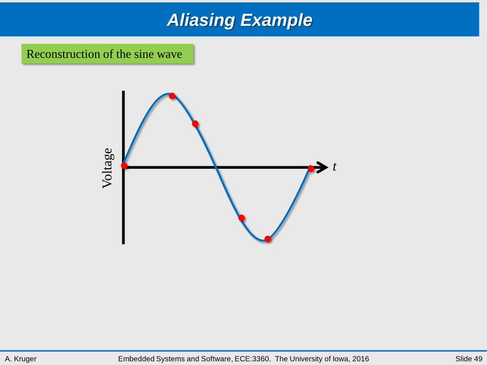
Aliasing Example

The points below are the samples from a sine wave

t

Vo

ltag

e


Aliasing Example

Reconstruction of the sine wave

t

Vo

ltag

e


Aliasing Example

But why not this reconstruction?

t

Vo

ltag

e


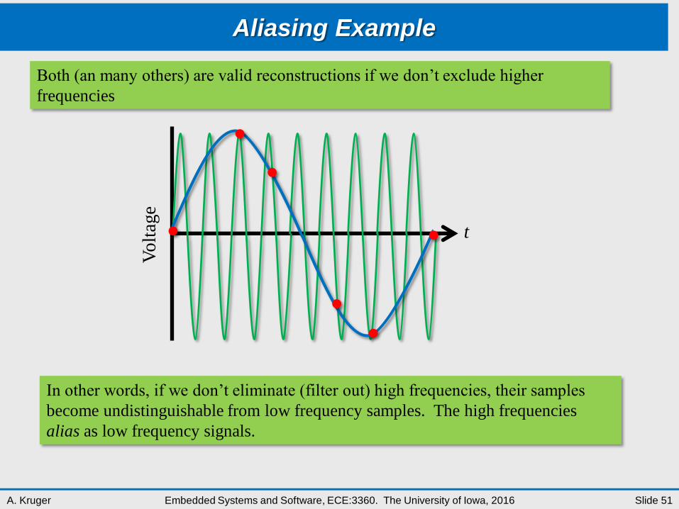
Aliasing Example

Both (an many others) are valid reconstructions if we don’t exclude higher

frequencies

In other words, if we don’t eliminate (filter out) high frequencies, their samples

become undistinguishable from low frequency samples. The high frequencies

alias as low frequency signals.

t

Vo

ltag

e


Aliasing Example

Sampling at 2.5 Hz (period = 0.4 s) the following signals are indistinguishable

tty 6sin)(

tty sin)(

Frequency f = 3 Hz

Frequency f = 0.5 Hz

In fact, with sampling frequency of 2.5 Hz one can only correctly sample signal

below the Nyquist frequency 2.5/2 = 1.25 Hz.


• Inherent delay in processing

– Actuation occurs later than expected

• Need to characterize implementation delay to make sure

it is negligible

• Hardware delay is usually easy to characterize

– Synchronous design

• Software delay is harder to predict

– Should organize code carefully so delay is predictable and

minimized

– Write software with predictable timing behavior (be like hardware)

Time Trigger Architecture

Synchronous Software Language and/or RTOS

Computation Delay

Documents

A Simple Introduction to Embedded Control Systems …s-iihr64.iihr.uiowa.edu/MyWeb/Teaching/ECE3360_2016/Lectures/PID... · A Simple Introduction to Embedded Control ... –F. Vahid