A Recursive Algorithm for Calculating the Relative Convex Hull

Gisela KletteAUT UniversityComputing & Mathematical SciencesAuckland, New Zealand

Motivation

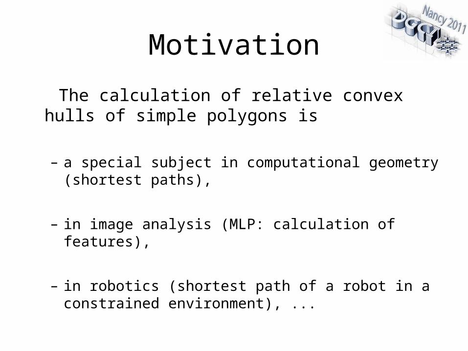
The calculation of relative convex hulls of simple polygons is

– a special subject in computational geometry (shortest paths),

– in image analysis (MLP: calculation of features),

– in robotics (shortest path of a robot in a constrained environment), ...

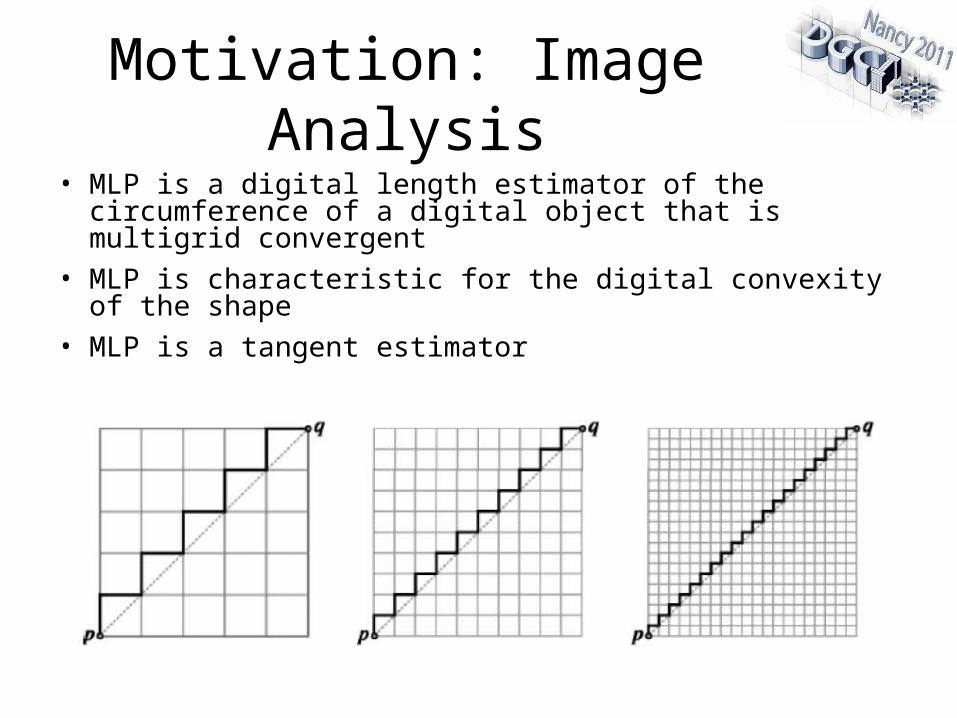
Motivation: Image Analysis• MLP is a digital length estimator of the circumference of

a digital object that is multigrid convergent

• MLP is characteristic for the digital convexity of the shape

• MLP is a tangent estimator

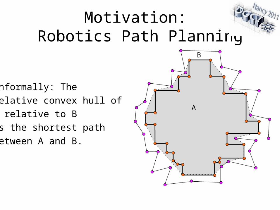
Motivation: Robotics Path Planning

Informally: The

relative convex hull of

A relative to B

is the shortest path

between A and B.

A

B

Definition 1

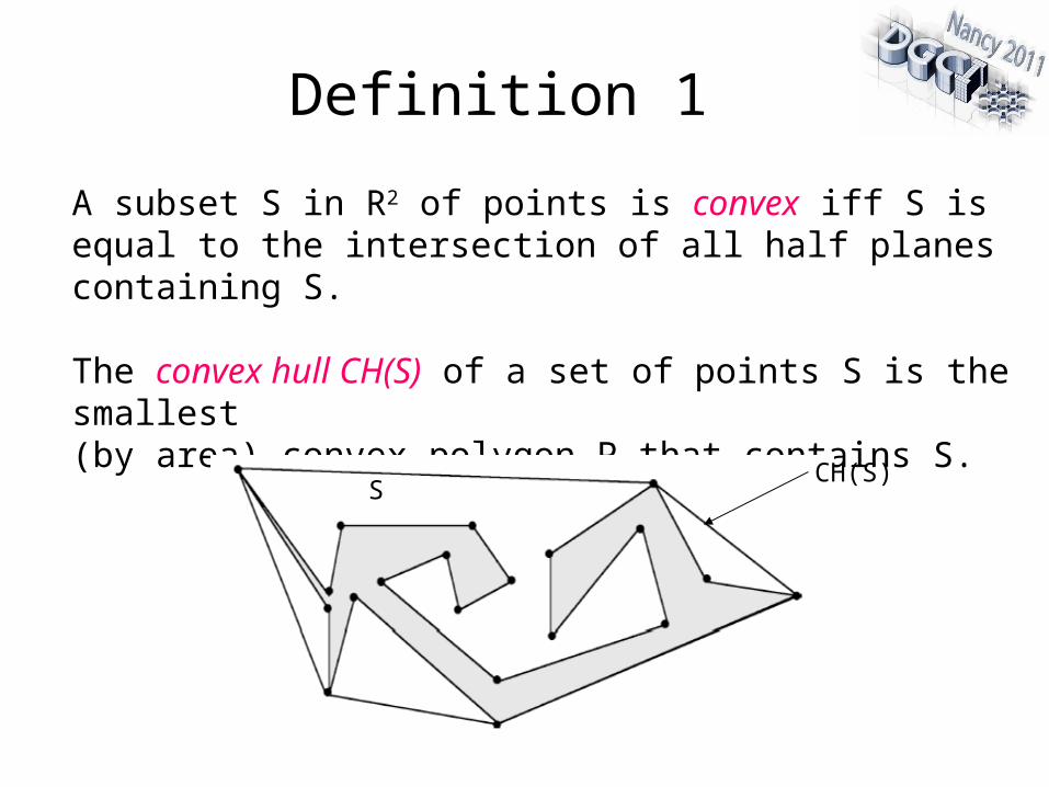
A subset S in R2 of points is convex iff S is equal to the intersection of all half planes containing S.

The convex hull CH(S) of a set of points S is the smallest (by area) convex polygon P that contains S.

SCH(S)

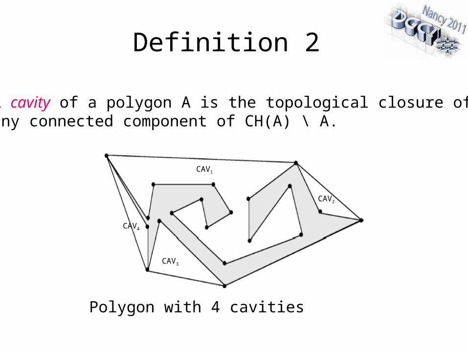
A cavity of a polygon A is the topological closure of any connected component of CH(A) \ A.

Definition 2

Polygon with 4 cavities

CAV1

CAV2

CAV3

CAV4

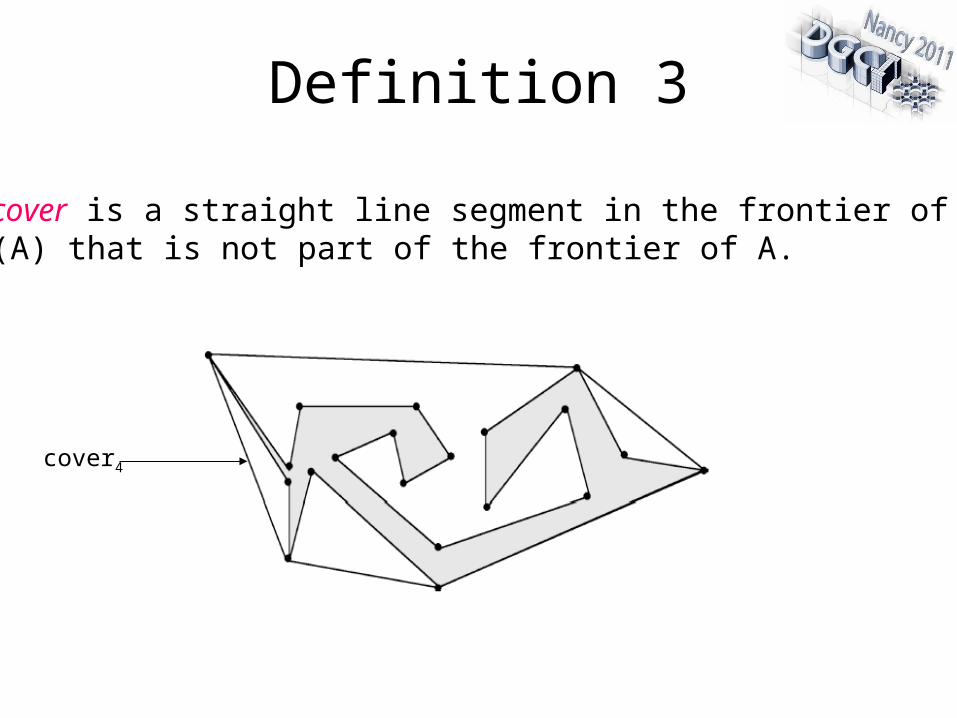
Definition 3

A cover is a straight line segment in the frontier of CH(A) that is not part of the frontier of A.

cover4

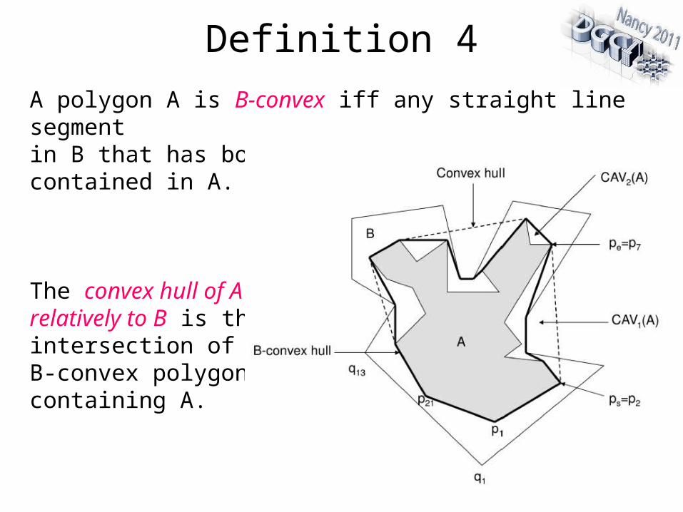
Definition 4

A polygon A is B-convex iff any straight line segmentin B that has both end points in A, is also contained in A.

The convex hull of A relatively to B is the intersection of all B-convex polygons containing A.

Definition 5

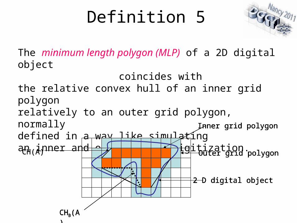
The minimum length polygon (MLP) of a 2D digital object coincides with the relative convex hull of an inner grid polygon relatively to an outer grid polygon, normallydefined in a way like simulating an inner and outer Jordan digitization.

Inner grid polygon

Outer grid polygon

2 D digital object

CH(A)

CHB(A)

Inner grid polygon

Outer grid polygon

2 D digital object

CH(A)

CHB(A)

Inner grid polygon

Outer grid polygon

2 D digital object

CHB(A)

Inner grid polygon

Outer grid polygon

2 D digital object

CHB(A)

Properties of MLP

- The inner and the outer polygon of a Jordan digitization have the constraint that they are at Hausdorff distance 1.

- Mappings exist between vertices and between cavities in A and in B.

- Convex vertices of the inner polygon and concave vertices of the outer polygon are candidates for the MLP.

- MLP is uniquely defined for a given digitized object

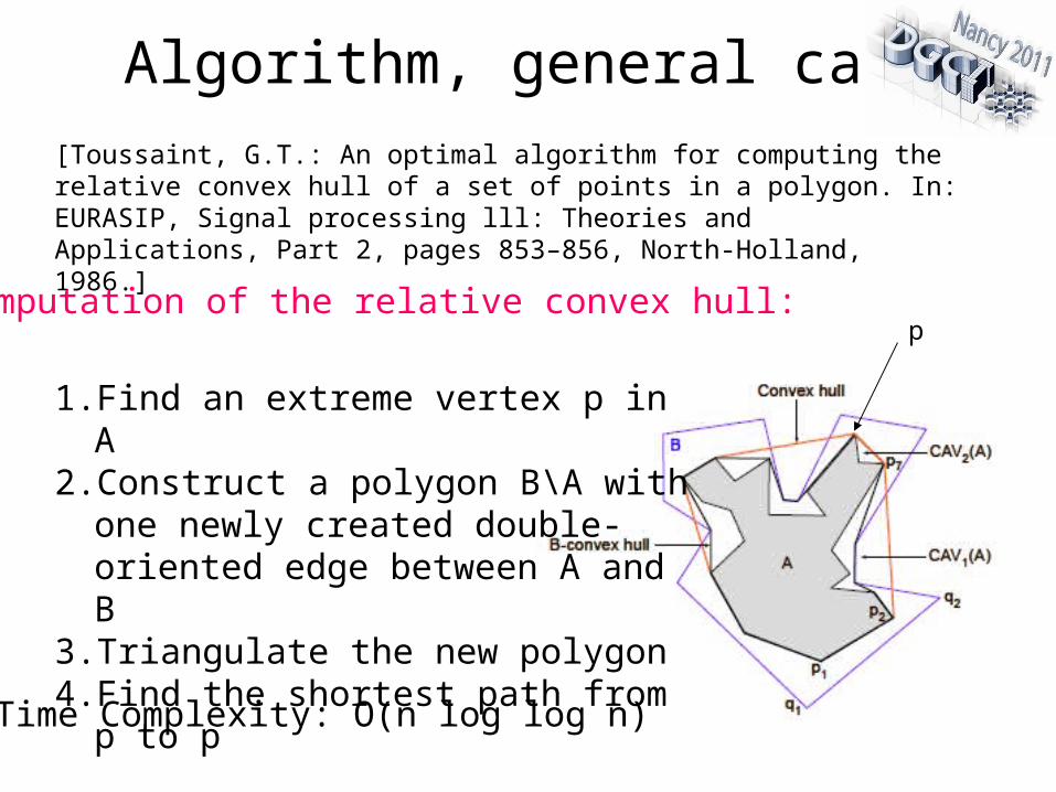
p

Algorithm, general case[Toussaint, G.T.: An optimal algorithm for computing the relative convex hull of a set of points in a polygon. In: EURASIP, Signal processing lll: Theories and Applications, Part 2, pages 853–856, North-Holland, 1986.]

1. Find an extreme vertex p in A 2. Construct a polygon B\A with one

newly created double-oriented edge between A and B

3. Triangulate the new polygon4. Find the shortest path from p to p

Time Complexity: O(n log log n)

Computation of the relative convex hull:

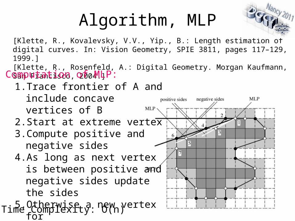
Algorithm, MLP[Klette, R., Kovalevsky, V.V., Yip., B.: Length estimation of digital curves. In: Vision Geometry, SPIE 3811, pages 117–129, 1999.][Klette, R., Rosenfeld, A.: Digital Geometry. Morgan Kaufmann, San Francisco, 2004.]

1. Trace frontier of A and include concave vertices of B

2. Start at extreme vertex3. Compute positive and negative

sides4. As long as next vertex is

between positive and negative sides update the sides

5. Otherwise a new vertex for CHB(A) has been found

Time Complexity: O(n)

Computation of MLP:

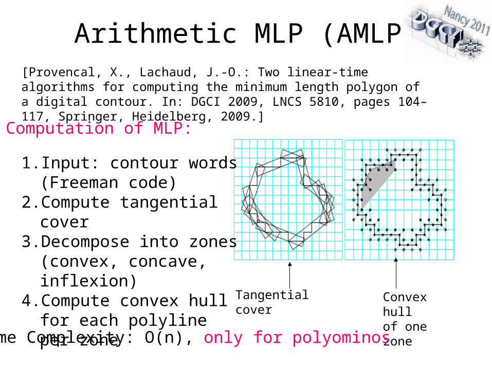
Tangential cover Convex hull of one zone

Arithmetic MLP (AMLP)[Provencal, X., Lachaud, J.-O.: Two linear-time algorithms for computing the minimum length polygon of a digital contour. In: DGCI 2009, LNCS 5810, pages 104–117, Springer, Heidelberg, 2009.]

1. Input: contour words (Freeman code)

2. Compute tangential cover3. Decompose into zones

(convex, concave, inflexion)4. Compute convex hull for

each polyline per zone

Time Complexity: O(n), only for polyominos

Computation of MLP:

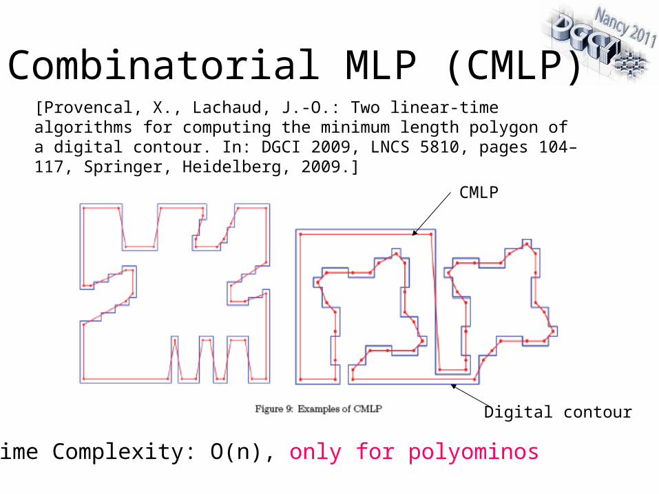
[Provencal, X., Lachaud, J.-O.: Two linear-time algorithms for computing the minimum length polygon of a digital contour. In: DGCI 2009, LNCS 5810, pages 104–117, Springer, Heidelberg, 2009.]

Combinatorial MLP (CMLP)

CMLP

Digital contour

Time Complexity: O(n), only for polyominos

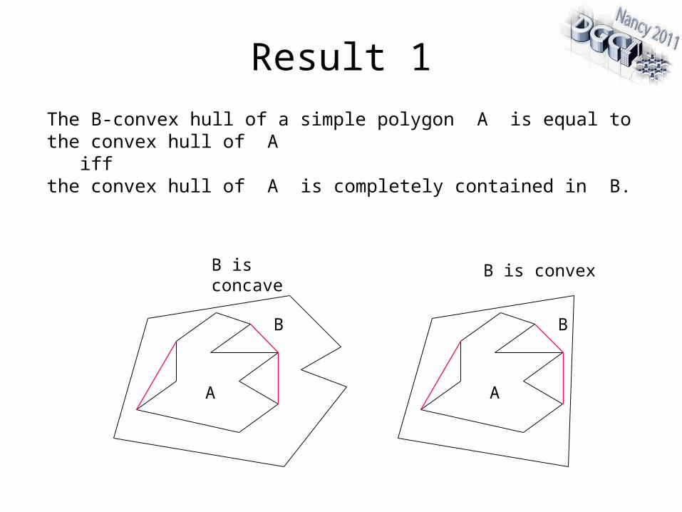
Result 1

The B-convex hull of a simple polygon A is equal to the convex hull of A iff the convex hull of A is completely contained in B.

A

B

A

B

B is concave B is convex

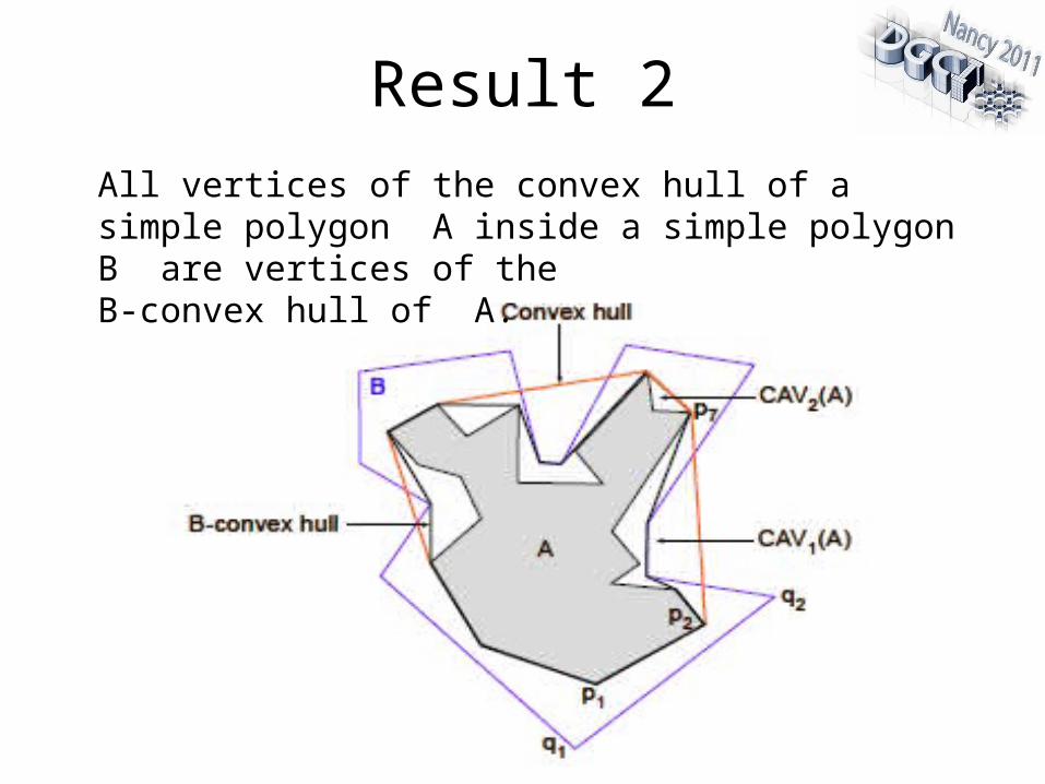
Result 2

All vertices of the convex hull of a simple polygon A inside a simple polygon B are vertices of the B-convex hull of A.

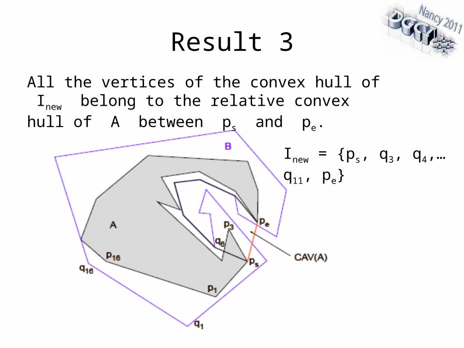
Result 3

All the vertices of the convex hull of Inew belong to the relative convex hull of A between ps and pe.

Inew = {ps, q3, q4,…q11, pe}

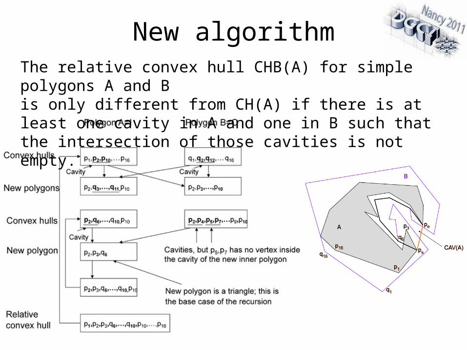
New algorithmThe relative convex hull CHB(A) for simple polygons A and B is only different from CH(A) if there is at least one cavity in A and one in B such that the intersection of those cavities is not empty.

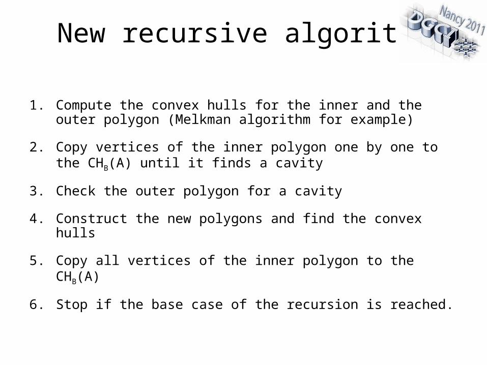
New recursive algorithm

1. Compute the convex hulls for the inner and the outer polygon (Melkman algorithm for example)

2. Copy vertices of the inner polygon one by one to the CHB(A) until it finds a cavity

3. Check the outer polygon for a cavity

4. Construct the new polygons and find the convex hulls

5. Copy all vertices of the inner polygon to the CHB(A)

6. Stop if the base case of the recursion is reached.

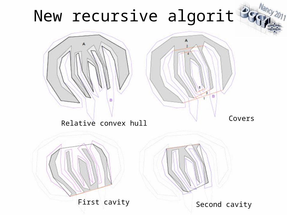
New recursive algorithm

Relative convex hullCovers

First cavity Second cavity

Discussion1. Recursive algorithm works for arbitrary simple polygons A

and B in O(n2), worst case.

2. It is a recursive procedure that is very simple and of low time complexity.

3. The algorithm runs in linear time if the maximum depth of stacked cavities of A is limited by a constant. We continue to study the expected time complexity of the algorithm under some general assumptions of variations (i.e., distribution) for possible input polygons A and B.

4. The depth of stacked cavities could be used as a shape descriptor.