A Physics Informed Neural Network Approach to Solution andIdentification of Biharmonic Equations of Elasticity

M. Vahaba, E. Haghighatb,1, M. Khaleghid, N. Khalilia

aSchool of Civil and Environmental Engineering, The University of New South Wales, Sydney 2052, AustraliabMassachusetts Institute of Technology, Cambridge, MA, USA

cUniversity of British Columbia, Vancouver, BC, CanadadDepartment of Civil Engineering, Center of Excellence in Structures and Earthquake Engineering, Sharif University of

Technology, Tehran, Iran

Abstract

We explore an application of the Physics Informed Neural Networks (PINNs) in conjunction with Airy stress

functions and Fourier series to find optimal solutions to a few reference biharmonic problems of elasticity

and elastic plate theory. Biharmonic relations are fourth-order partial differential equations (PDEs) that are

challenging to solve using classical numerical methods, and have not been addressed using PINNs. Our work

highlights a novel application of classical analytical methods to guide the construction of efficient neural

networks with the minimal number of parameters that are very accurate and fast to evaluate. In particular,

we find that enriching feature space using Airy stress functions can significantly improve the accuracy of

PINN solutions for biharmonic PDEs.

Keywords: Physics-informed neural network; Biharmonic equations; Theory of elasticity; Elastic thinplates

1. Introduction

Deep learning (DL) has become a thriving framework that manifest in various fields including speech/

handwriting recognition [1], image processing/classification [2], medical diagnoses [3], and fundamental

scientific researches [4]. In engineering and science, DL has emerged as a promising alternative to emulate

and capture the patterns, at primitive levels, as well as to predict complicated challenging interactive

scenarios, at best, which is both evenly cumbersome and extremely time consuming to the cutting-edge

simulators. DL is elaborated successfully in an increasing number of areas, including geo/material sciences

[5–7], solid/fluid/thermo mechanics [8–17], and reservoir/electrical/chemical engineering [18–24], to name a

few.

A common difficulty with the state-of-the-art machine learning (ML) techniques has been due to the

extremely complex and expensive data acquisition in a vast majority of complex engineering / scientific

systems [25]. This threatens the feasibility and reliability of machine learning and renders conclusion and

decision making a formidable task, if not impossible. A promising remedy in dealing with such problems

is the prior physical knowledge, typically accessible in forms of Ordinary/Partial Differential Equations

(i.e., ODEs/PDEs), which plays the role of a regularization agent to consolidate the admissibility of the

∗Corresponding author:Email address: ehsanh@mit.edu (E. Haghighat)

Preprint submitted to ASCE August 17, 2021

arX

iv:2

108.

0724

3v1

[cs

.LG

] 1

6 A

ug 2

021

solution, despite access to limited data. The first glimpse of the promising performance of prior information

embedded deep learning in solution and discovery of high-dimensional PDEs has been due to the very

recent contributions by Owhadi [26], Han et al. [27], Bar-Sinai et al. [28], Rudy et al. [29], and Raissi

et al. [30], which is now known as Physics-Informed Neural Networks (PINNs). PINNs are constructed

and trained on the basis of a series of loss functions, endowed with the system of ODEs/PDEs and the

corresponding Dirichlet / Neumann Boundary Conditions (BCs) or Initial Values (IVs), which govern the

problem under consideration. PINNs are privileged in comparison to the preceding endeavors in the inclusion

of the prior information as a result of the appropriate choice of network architecture, algorithmic advances

(e.g., graph-based automated differentiation [31]), and software developments (e.g., TensorFlow [32], Keras

[33]). Recently, PINNs has been successfully applied to the solution and discovery in fluid [34, 35, 35–

37]/solid [38–42]/pore [43–46]/thermo mechanics [10, 47], Eikonal equations [48] (for a detailed review, see

[49]).

In this study, we emphasize the novel elaboration of PINNs to the solution of a range of benchmark

examples from the theory of elasticity and elastic plates, governed by the fourth-order Biharmonic equation.

In the context of PINNs, the space of admissible solutions is approximated by general multi-layer neural

networks, and the solution strategy is to minimize a loss function that includes the Mean-Squared Error

norm (MSE) of the governing differential equations in conjunction with the complementary BCs/IVs, across

randomly selected sampling points. The inherent capabilities of PINNs are explored with the discovery of

parametric solutions based on the analytical closed-form solutions in the theory of elasticity. We examine

the performance of PINNs in the solution and parametric study of elastic thin plates subjected to external

loading. We find that, while setting up PINNs for different problems is relatively straightforward, training

PINNs to reach a desired level of accuracy is an extremely hard problem. There are two reasons for such

a poor performance; first, is associated with the use of first-order optimization methods; and second, with

neural network architecture. However, we find that if we custom-design the network with features leveraged

from the classical analytical solutions of the Biharmonic equation, including Airy functions and Taylor series,

we can improve their performance significantly.

The paper is organized as follows: In section 2, we briefly describe the fundamentals of PINNs. In section

3, we elaborate PINNs in the solution of the Lame problem and semi-infinite foundation, which are two well-

known benchmark problems in the theory of elasticity. Section 4 is dedicated to the application of PINNs

to the study of a selection of problems from the theory of elastic plates. Concluding remarks are presented

in section 5. All examples presented in the current study are open-accessed and can be downloaded from

https://github.com/sciann/sciann-applications.

2. Physics-Informed Neural Networks

Over the past few decades, abundant efforts has been conducted in relation to predictive physical mod-

elling using machine learning approaches (e.g., support vector machines [50], Gaussian processes [51], feed-

forward [52]/convolutional [53]/recurrent neural networks [54]). Most classical approaches employ deep

learning as a black-box data-driven tool and demand a significant amount of data for training. This is com-

monly conceived as a big drawback for engineering applications due to restrictions with data accessibility,

validity, noises, and other uncertainties. A beneficial remedy has been achieved thanks to the pioneering

so-called physics-informed neural networks (PINNs), which embody the prior knowledge – typically in the

forms of ODEs/PDEs – into the training process. By exploiting a feed-forward architecture in conjunction

with Automatic Differentiation [31], the physics-informed neural networks are constructed and trained to

satisfy the underlying governing equations and, therefore, demand fewer data.

2

x u

Hidden layers

Input Output

Flow of data

connections

Figure 1: Standard PINN architecture, defining the mapping u : x 7→ Nu(x;W, b).

Let us consider a steady state partial differential operator P applied on a scalar solution variable u,

i.e., Pu(x) = f(x), subjected to the boundary condition Bu(∂x) = g(∂x), with x ∈ Rd and d as the

spatial dimension of the problem. According to the PINNs, the solution variable u is approximated using

a feed-forward neural network, with inputs x and outputs u. Consider a nonlinear map Σ defined as

Σi(xi) := yi = σi(W i · xi + bi), with W , b as weights and baiases of this transformation, and σ as a

nonlinear transformer. Such a nerual network is then expressed mathematically as

u = ΣL ΣL−1 · · · Σ0(x) (1)

where represents the compositional construction of the network and pictured graphically in Fig.1. Such

a network defines a mapping between input and output variables. W i, bi form parameters of this trans-

formation, equivalent to the degrees of freedom in a finite element discretization, and are all collected in

θ =⋃Li=0(W i, bi). For the internal layers, hyperbolic-tangent is often used as the nonlinear transformer σi,

a.k.a. activation function, and for the last layer, it is often kept linear for regression-type problems, which

we account here.

According to the PINNs, the parameters of this neural network are identified by minimizing a multi-

objective loss function, consisted of the error associated with PDE residual and boundary conditions, and

it is constructed as

L(x;θ) =∑

λiLi = λ1 ‖Pu− 0‖Ω + λ2 ‖Bu− g‖∂Ω + . . . (2)

where L is a loss function. Since we deal with regression type problems, the mean squared error norm is

used as the loss function, i.e., ‖‖ = MSE(). Note λi’s are weights associated with each loss term. The

optimal values of the networks parameters, i.e., θ∗, are then identified by optimizing this loss function as

θ∗ = arg minθ∈RD

L(X;θ) (3)

3

with D as the total number of trainable parameters, and X ∈ RN×d is the set of N collocation points used

to optimize this loss function.

As we find, to evaluate the loss function (2), we need to evaluate derivatives of the u at different training

points. Instead of numerical differentiation used in earlier works, PINNs leverage automatic differentiation

that is readily available in modern deep learning frameworks [33]. This enables the explicit inclusion of any

partial differential operator P or Neumann boundary conditions acting on the field variable u.

In this study, we use the open-source python API SciANN [34], to set up and train the PINN architectures.

SciANN is optimized to perform scientific machine learning with minimal effort. Implemented on the reputed

deep-learning packages Tensorow [32] and Keras [33], it inherits their functionalities in terms of graph-based

automatic differentiation and high-performance computing. For the problems showcased in the following

sections, unless stated otherwise, training is carried out using the Adam optimization scheme [55]. The

network hyperparameters such as the number of nodes per layer or the number of hidden layers are described

separately for each problem.

3. PINN Solution of Elasticity Problems

In this section, PINNs are employed to the solution of problems in the theory of elasticity. The partial

differential equation of the Airy stress function, as a robust solution procedure in the theory of elasticity, is

briefly explained and is applied for the solution of two benchmark examples in the field.

3.1. Theory of Elasticity

In the theory of elasticity, the solution field can be obtained by utilizing a variety of stress functions.

The Airy stress function [56] is a simplified form of the more general Maxwell stress function [57], which

was originally introduced for the solution of two-dimensional elasticity problems. The idea was to develop

a series of scalar representative stress functions, that simultaneously satisfy the equilibrium equation and

compatibility requirements [58, 59]. Neglecting the body forces, for the sake of simplicity in presentation, it

follows that [60]

∇4φ =

(∂2

∂r2+

1

r

∂

∂r+

1

r2

∂2

∂θ2

)(∂2

∂r2+

1

r

∂

∂r+

1

r2

∂2

∂θ2

)φ = 0, (4)

in which φ is the Airy stress function in polar coordinate system, i.e., (r, θ). Alternatively, this equation can

be expressed in the Cartesian coordinate system as

∇4φ =

(∂2

∂x2+

∂2

∂y2

)(∂2

∂x2+

∂2

∂y2

)φ = 0, (5)

where (x, y) = r(sinθ, cosθ). The above relation is called biharmonic equation which describes the in-plane

elasticity problems with a unified expression. Eq. (4) can be solved in conjunction with adequate boundary

conditions over ∂Ω. Using the Airy stress function, the stress components can be determined as

σr =1

r

∂φ

∂r+

1

r2

∂2φ

∂θ2,

σθ =∂2φ

∂r2,

σrθ = − ∂

∂r

(1

r

∂φ

∂θ

).

(6)

4

op

ipir

or

,

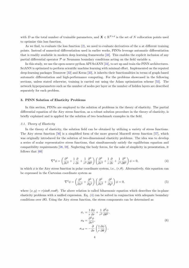
Figure 2: Lame problem setup, subjected to internal and external boundary conditions pi and po, respectively.

Using the Hooke’s law, the strain components are expressed as

εr =1

2µ

(σr −

1

4(3− κ)(σr + σθ)

),

εθ =1

2µ

(σθ −

1

4(3− κ)(σr + σθ)

),

εrθ =1

2µσrθ,

(7)

where κ is 3−4ν or (3−ν)/(1+ν) for plane strain or plane stress state, respectively. In the above relations,

µ is Lame’ second parameter (identical to the shear modulus, i.e., G), and ν is Poisson’s ratio.

3.2. Lame Problem

In this example, the application of PINNs to the solution of circular annulus subjected to uniform

external/internal pressure is illustrated (see Fig. 2), which is known as Lame problem [61]. Considering the

axisymmetry of the problem, the solution is independent of θ. This, in turn, leads to a simplified form of

the biharmonic equation (i.e., Eq. (4)) as

∇4φ =

(∂2

∂r2+

1

r

∂

∂r

)(∂2

∂r2+

1

r

∂

∂r

)φ = 0. (8)

The problem definition is accomplished by the introduction of the boundary conditions as σr(r = ri, θ) = pi

and σr(r = ro, θ) = po, with pi and po being the pressure exerted towards the internal and external faces of

the annulus, respectively.

In the theory of elasticity, it is shown that the solution to biharmonic Eq. (8) on the basis of the

above-mentioned boundary conditions is multi-valued. In order to circumvent this difficulty, the so-called

5

consistency constraints of the displacement field need to be incorporated. A beneficial constraint is imposed

through the definition of strains versus displacement field as [58]

εr =∂ur∂r

,

εθ =urr

+∂uθr∂θ

.

(9)

Due to the axisymmetry of the problem, the tangential displacement uθ must yield the identical values

independent of θ, or simply vanish (i.e., uθ ≡ 0).

Here, the solution to Lame problem is investigated for pi = 1 MPa and po = 2 MPa by means of the

PINNs. Suppose the domain is delimited to ri = 1 m and ro = 2 m, with material properties set to

G = 100 GPa and ν = 0.25. To this end, it is required to define the unknown solutions using the below

1 1.2 1.4 1.6 1.8 20.5

1

1.5

2

2.5

r(m)

σr(M

Pa)

Neural Network Solution

Airy-Network Solution

Reference Solution

(a)

1 1.2 1.4 1.6 1.8 2

10−8

10−6

10−4

10−2

100

r(m)

|σr−σ∗ r|(

MP

a)

Neural Network Solution

Airy-Network Solution

(b)

0 2,000 4,000 6,000 8,000 10,000

10−10

10−8

10−6

10−4

10−2

100

Epoch

L/L0

Neural Network Solution

Airy-Network Solution

(c)

Figure 3: Deep learning solution for Lame problem; a) profile of radial stresses σr, b) error norm of radial stresses, c) networktraining history.

6

neural networks

φ(r) ' Nφ(r),

ur ' Nur(r).

(10)

Notably, the inclusion of the displacement field in the neural network architecture facilitates the imposition

of the boundary conditions related to the consistency constraint in the strain field. The physics-informed

loss terms of the total cost function are defined as

LΩ =

∥∥∥∥( ∂2

∂r2+

1

r

∂

∂r

)(∂2

∂r2+

1

r

∂

∂r

)φ

∥∥∥∥ ,Lε =

∥∥∥∥ 1

2µ

(rσθ −

1

4(3− κ)(σr + σθ)

)− ur

∥∥∥∥ ,L∂Ω1

= λ1 ‖(σr − pi) (r = rmin)‖ ,L∂Ω2 = λ2 ‖(σr − po) (r = rmax)‖ .

(11)

Training is performed over 2000 sampling points (same as batch size) through 10000 epochs. It is noteworthy

that in the above relation λi’s are mini-batch optimization parameters, which are set to relatively large values

to guarantee consistent optimization on the boundaries.

As per the approximation functions for the unknown variables φ and ur, two approaches are taken.

In the first approach, they are approximated using two neural networks, which consists of 5 hidden layers

and 20 neurons per layer, with hyperbolic-tangent utilized as the activation function. In the second ap-

proach, the Airy stress functions are adopted to construct the optimal approximation space. Therefore, the

approximation function takes the form of

φ(r) = a1logr + a2r2logr + a3r

2 + a4,

ur(r) =1

E(−a1

r+ 2a2rlogr + 2a3r)−

ν

Eφ,

(12)

in which ai’s are the only parameters of the optimization problem, identified by minimizing the same

physics-informed loss function.

The results are presented in Fig. 3, where λ1 and λ2 are preset to large numbers λ1 = λ2 = 100 so as

to accurately enforce the boundary conditions. In this regard, the profiles of the radial stress component

σr and its absolute error with respect to the exact values (i.e., σ∗r ) are shown for the PINNs solution and

compared against the analytical solution in the theory of elasticity [58]. Excellent agreement is observed

between the present model and the reference solution, which demonstrates the capabilities of the PINNs in

the solution of higher-order ODEs. In Fig. 3c, the evolution of normalized loss versus epochs is depicted,

which indicates the rapid convergence in the training of PINNs for the Lame problem. It is evident from the

solutions that the Airy-network results in superior convergence and accuracy characteristics, and therefore

is the optimal choice for solving the Lame problem. It should also be noted that due to the small number of

parameters of the Airy-network, the optimization time per epoch is much faster than the case of the neural

network, which is summed up to at least 10 times greater efficiency in total training duration.

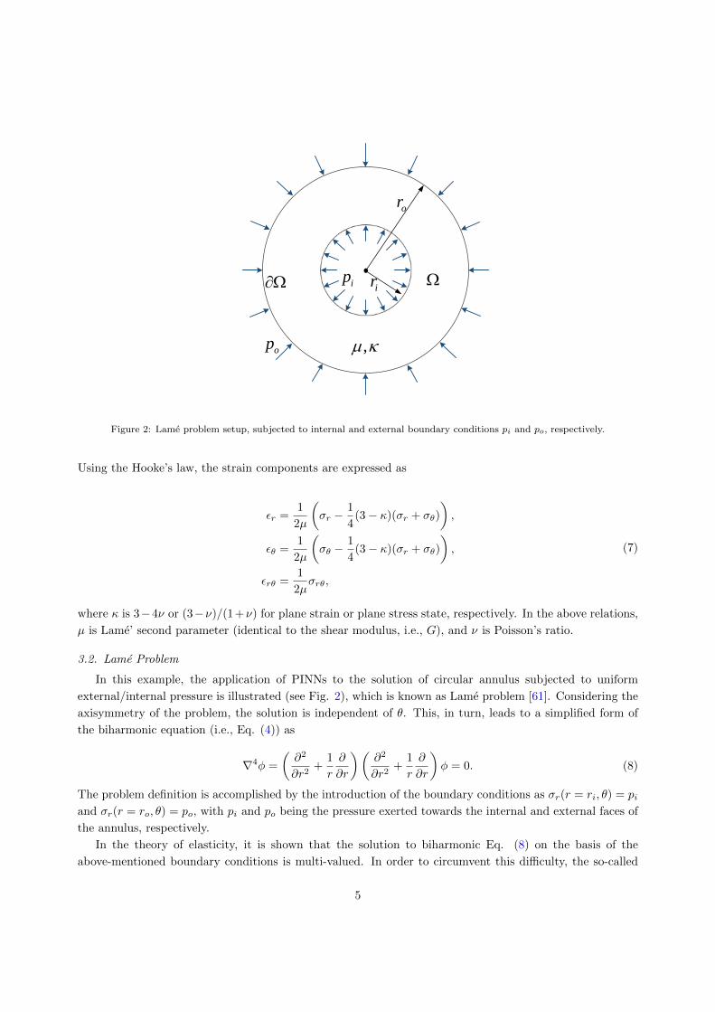
3.3. Foundation

As the second case, we investigate the solution of a half-space subjected to uniform pressure over a finite

interval of its boundary using PINNs, which is representative of a strip foundation. In the theory of elasticity,

7

q

,

Oy

x

l

(a) Finite pressure

r

q

,

Oq

O

r

(b) Infinite pressure

Figure 4: Problem definition for half-space subject to strip footing; a) Geometry and boundary conditions, b) Intermediatesolutions.

this problem is solved through the superposition of two half-spaces subjected to shifted semi-infinite uniform

pressure along one-half of its boundary –in reverse directions –as shown in Fig. 4. Accordingly, the Airy

stress function for the solution to half-space subjected to uniform pressure q is defined as φ = qr2f(θ) [58].

Inserting this definition into the biharmonic Eq. (4) yields

∇4φ =1

r2

∂2

∂θ2

(∂2f(θ)

∂θ2+ 4f(θ)

)= 0. (13)

Here, the PINNs is applied to obtain the solution for q = 1 kPa using the Airy-network architecture

φ(r, θ) ' qr2Nθ(θ). Alternatively, the physics-informed solution to the general form of the biharmonic

equation in the Cartesian coordinate system (i.e., Eq. (5)) is elaborated to construct a more general

neural network to solve this problem. It is noteworthy that the description of the biharmonic Equation

in Cartesian coordinates is preferred over the polar coordinates description (i.e., Eq. (4)) to avoid the

problematic singularity of the equations with respect to r at the origin. As a remedy in this example, the

order of the biharmonic Eq. (5) is reduced through the change of variables as

∇2ψ =

(∂2

∂x2+

∂2

∂y2

)ψ = 0,

ψ =

(∂2

∂x2+

∂2

∂y2

)φ.

(14)

In this fashion, two conjugate neural networks, i.e., φ(x, y) ' Nφ(x, y) and ψ(x, y) ' Nψ(x, y), are employed

to solve the biharmonic equation. For the sake of comparison a solo neural network, i.e., φ(x, y) ' Nφ(x, y),

is also exercised by using the fourth-order form of the biharmonic equation. In all cases, 6 hidden layers

with 20 neurons per layer are supposed for the construction of the neural networks, where the loss terms of

the total cost function are described as

LΩ =∥∥∇4φ

∥∥ ,L∂Ω1

= λ1 ‖(σθ − q) (θ = θmax)‖ ,L∂Ω1

= λ2 ‖σθ (θ = θmin)‖ ,L∂Ω1

= λ3 ‖σrθ (θ = θmax)‖ ,L∂Ω1

= λ4 ‖σrθ (θ = θmin)‖ .

(15)

8

0 200 400 600 800 1,000

10−10

10−8

10−6

10−4

10−2

100

Epoch

L/L0

0 500 1,000 1,500 2,000

10−10

10−8

10−6

10−4

10−2

100

Time (s)

L/L0

Solo Network

Conjugate Networks

Airy Network

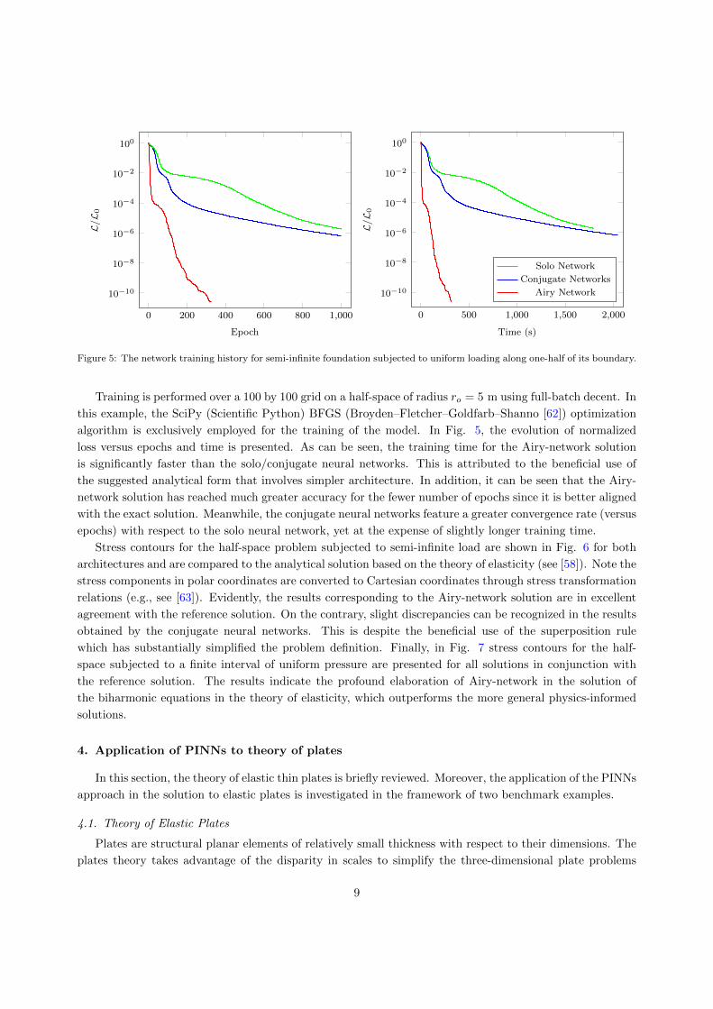
Figure 5: The network training history for semi-infinite foundation subjected to uniform loading along one-half of its boundary.

Training is performed over a 100 by 100 grid on a half-space of radius ro = 5 m using full-batch decent. In

this example, the SciPy (Scientific Python) BFGS (Broyden–Fletcher–Goldfarb–Shanno [62]) optimization

algorithm is exclusively employed for the training of the model. In Fig. 5, the evolution of normalized

loss versus epochs and time is presented. As can be seen, the training time for the Airy-network solution

is significantly faster than the solo/conjugate neural networks. This is attributed to the beneficial use of

the suggested analytical form that involves simpler architecture. In addition, it can be seen that the Airy-

network solution has reached much greater accuracy for the fewer number of epochs since it is better aligned

with the exact solution. Meanwhile, the conjugate neural networks feature a greater convergence rate (versus

epochs) with respect to the solo neural network, yet at the expense of slightly longer training time.

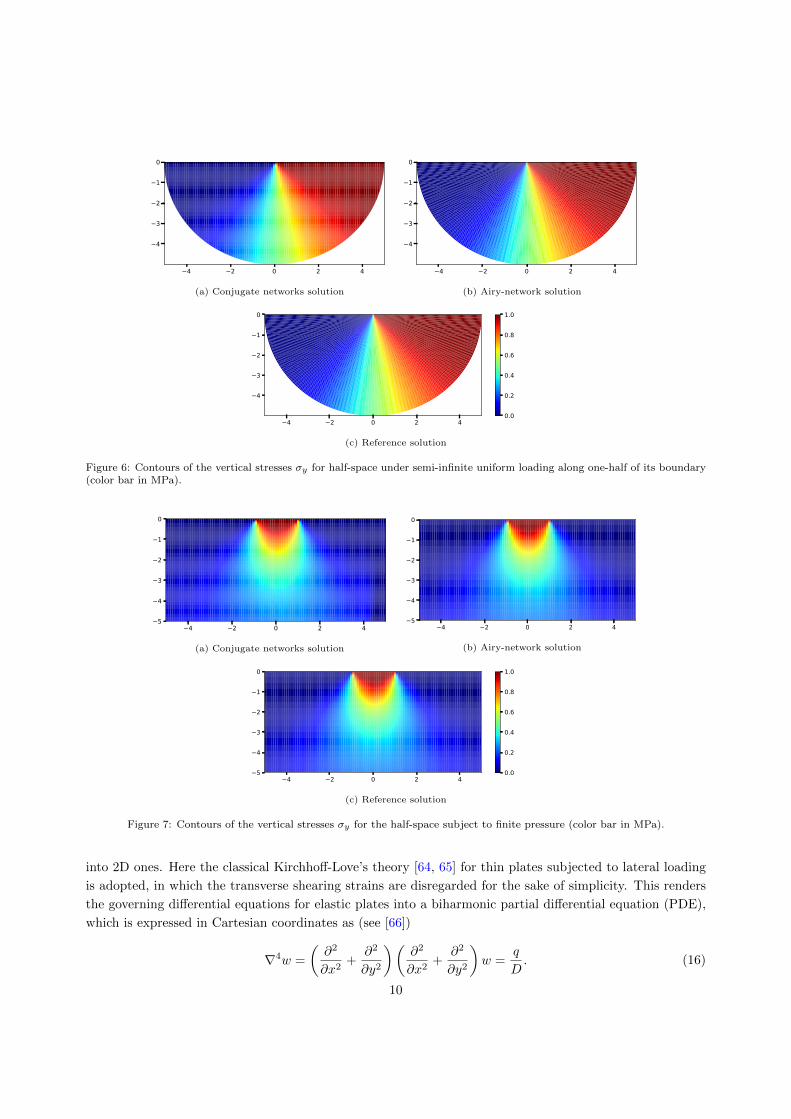
Stress contours for the half-space problem subjected to semi-infinite load are shown in Fig. 6 for both

architectures and are compared to the analytical solution based on the theory of elasticity (see [58]). Note the

stress components in polar coordinates are converted to Cartesian coordinates through stress transformation

relations (e.g., see [63]). Evidently, the results corresponding to the Airy-network solution are in excellent

agreement with the reference solution. On the contrary, slight discrepancies can be recognized in the results

obtained by the conjugate neural networks. This is despite the beneficial use of the superposition rule

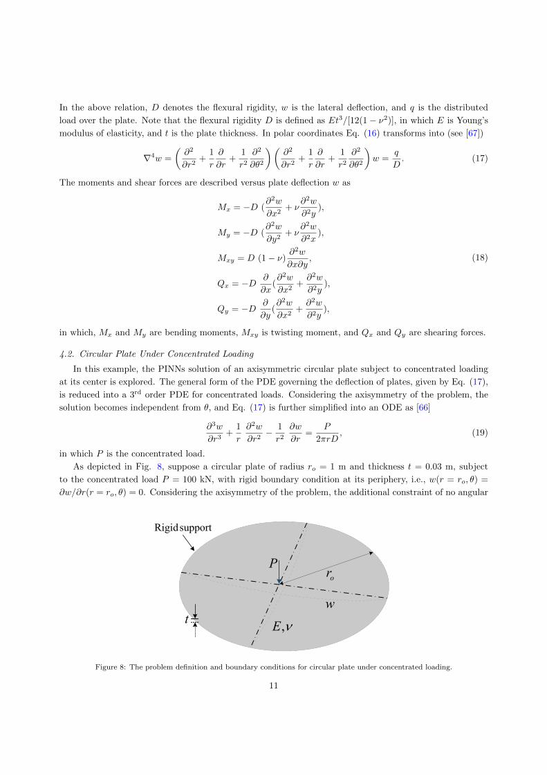
which has substantially simplified the problem definition. Finally, in Fig. 7 stress contours for the half-

space subjected to a finite interval of uniform pressure are presented for all solutions in conjunction with

the reference solution. The results indicate the profound elaboration of Airy-network in the solution of

the biharmonic equations in the theory of elasticity, which outperforms the more general physics-informed

solutions.

4. Application of PINNs to theory of plates

In this section, the theory of elastic thin plates is briefly reviewed. Moreover, the application of the PINNs

approach in the solution to elastic plates is investigated in the framework of two benchmark examples.

4.1. Theory of Elastic Plates

Plates are structural planar elements of relatively small thickness with respect to their dimensions. The

plates theory takes advantage of the disparity in scales to simplify the three-dimensional plate problems

9

4 2 0 2 4

4

3

2

1

0

0.0

0.2

0.4

0.6

0.8

1.0

(a) Conjugate networks solution

4 2 0 2 4

4

3

2

1

0

0.0

0.2

0.4

0.6

0.8

1.0

(b) Airy-network solution

4 2 0 2 4

4

3

2

1

0

0.0

0.2

0.4

0.6

0.8

1.0

(c) Reference solution

Figure 6: Contours of the vertical stresses σy for half-space under semi-infinite uniform loading along one-half of its boundary(color bar in MPa).

4 2 0 2 45

4

3

2

1

0

0.0

0.2

0.4

0.6

0.8

1.0

(a) Conjugate networks solution

4 2 0 2 45

4

3

2

1

0

0.0

0.2

0.4

0.6

0.8

1.0

(b) Airy-network solution

4 2 0 2 45

4

3

2

1

0

0.0

0.2

0.4

0.6

0.8

1.0

(c) Reference solution

Figure 7: Contours of the vertical stresses σy for the half-space subject to finite pressure (color bar in MPa).

into 2D ones. Here the classical Kirchhoff-Love’s theory [64, 65] for thin plates subjected to lateral loading

is adopted, in which the transverse shearing strains are disregarded for the sake of simplicity. This renders

the governing differential equations for elastic plates into a biharmonic partial differential equation (PDE),

which is expressed in Cartesian coordinates as (see [66])

∇4w =

(∂2

∂x2+

∂2

∂y2

)(∂2

∂x2+

∂2

∂y2

)w =

q

D. (16)

10

In the above relation, D denotes the flexural rigidity, w is the lateral deflection, and q is the distributed

load over the plate. Note that the flexural rigidity D is defined as Et3/[12(1− ν2)], in which E is Young’s

modulus of elasticity, and t is the plate thickness. In polar coordinates Eq. (16) transforms into (see [67])

∇4w =

(∂2

∂r2+

1

r

∂

∂r+

1

r2

∂2

∂θ2

)(∂2

∂r2+

1

r

∂

∂r+

1

r2

∂2

∂θ2

)w =

q

D. (17)

The moments and shear forces are described versus plate deflection w as

Mx = −D (∂2w

∂x2+ ν

∂2w

∂2y),

My = −D (∂2w

∂y2+ ν

∂2w

∂2x),

Mxy = D (1− ν)∂2w

∂x∂y,

Qx = −D ∂

∂x(∂2w

∂x2+∂2w

∂2y),

Qy = −D ∂

∂y(∂2w

∂x2+∂2w

∂2y),

(18)

in which, Mx and My are bending moments, Mxy is twisting moment, and Qx and Qy are shearing forces.

4.2. Circular Plate Under Concentrated Loading

In this example, the PINNs solution of an axisymmetric circular plate subject to concentrated loading

at its center is explored. The general form of the PDE governing the deflection of plates, given by Eq. (17),

is reduced into a 3rd order PDE for concentrated loads. Considering the axisymmetry of the problem, the

solution becomes independent from θ, and Eq. (17) is further simplified into an ODE as [66]

∂3w

∂r3+

1

r

∂2w

∂r2− 1

r2

∂w

∂r=

P

2πrD, (19)

in which P is the concentrated load.

As depicted in Fig. 8, suppose a circular plate of radius ro = 1 m and thickness t = 0.03 m, subject

to the concentrated load P = 100 kN, with rigid boundary condition at its periphery, i.e., w(r = ro, θ) =

∂w/∂r(r = ro, θ) = 0. Considering the axisymmetry of the problem, the additional constraint of no angular

Por

Rigidsupport

,E tw

Figure 8: The problem definition and boundary conditions for circular plate under concentrated loading.

11

0 2,000 4,000 6,000 8,000 10,00010−14

10−12

10−10

10−8

10−6

10−4

10−2

100

Epoch

L/L0

0 250 500 750 1,000 1,250

10−14

10−12

10−10

10−8

10−6

10−4

10−2

100

Time (s)

L/L0

Neural Network (Adam)

Neural Network (BFGS)

Parametric Network (Adam)

Parametric Network (BFGS)

Figure 9: Training data history for circular plate under concentrated loading.

deflection needs to be imposed to the problem at center, i.e., ∂w/∂r(r = 0, θ) = 0. The material properties

of the plate are set to: Young’s module of elasticity, E = 20 GPa; and Poisson’s ratio, ν = 0.25.

The solution is constructed by definition of w = Nw(r), using 10 hidden layers with 10 neurons per

layer. The network training is performed by using tanh as the activation function. Four loss functions are

introduced to set up the optimization problem as

LΩ =

∥∥∥∥r2 ∂3w

∂r3+ r

∂2w

∂r2− ∂w

∂r− Pr

2πD

∥∥∥∥ ,L∂Ω1

= λ1 ‖(∂w/∂r) (r = 0)‖ ,L∂Ω2 = λ2 ‖(∂w/∂r) (r = ro)‖ ,L∂Ω3

= λ3 ‖(w) (r = ro)‖ .

(20)

Note in the evaluation of domain losses LΩ, to annihilate singularities with respect to r at the origin, Eq.

(19) is multiplied by r2. As an alternative solution, for the case of uniform loading q, Eq. (17) can be

directly integrated into [68]

w = − qr4

64D+

1

4a1r

2 (ln r − 1) +1

4a2r

2 + a3 ln r + a4, (21)

where for the concentrated loading case considered here the distributed load is vanished (i.e., q = 0).

Note ai’s are the only parameters of the optimization problem identified exclusively by minimizing the loss

functions related to the boundary conditions. The parametric network solution requires the introduction of

an additional boundary condition related to shearing forces (i.e., L∂Ω4) to accommodate the inclusion of the

fourth unknown. Thus, the losses associated with the parametric solution are expressed as

L∂Ω1= λ1 ‖(∂w/∂r) (r = 0)‖ ,

L∂Ω2 = λ2 ‖(∂w/∂r) (r = ro)‖ ,L∂Ω3

= λ3 ‖(w) (r = ro)‖ ,L∂Ω4 = λ4‖Qr − P/(2π r)‖,

(22)

where,

Qr = D(∂3w/∂r3 + (1/r) ∂2w/∂r2 − (1/r2) ∂w/∂r

). (23)

12

Considering the singularity of Eqs. (21) to (23) with respect to r at origin, r = 0 is excluded from the

training of the parametric network.

Training is performed by means of a uniform grid consisting of 100 coalition points and the batch size

of 32. Here, the Adam and BFGS optimisation schemes are elaborated for the training. The convergence

history versus epochs and training time is plotted for the both networks in Fig. 9. Evidently, the BFGS

scheme has outperformed the Adam algorithm in all cases. The convergence profile of the parametric network

represents excellent convergence rate, that has reached at machine precision within relatively lesser epochs.

In contrast, the relative error norm associated with the neural network solution lies in the range of 10−4 to

10−5, even beyond much more epochs (e.g., up to 10,000 epochs in the Adam scheme). This coincides with

the longer training time required in the neural network solution.

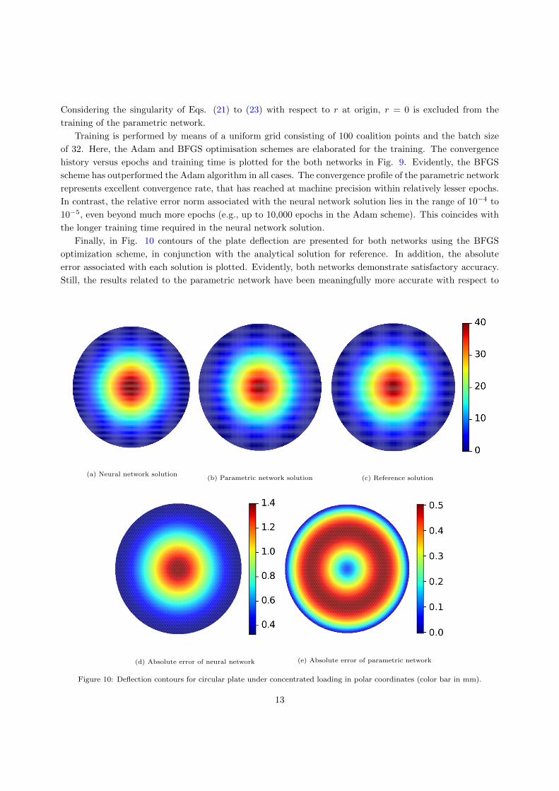
Finally, in Fig. 10 contours of the plate deflection are presented for both networks using the BFGS

optimization scheme, in conjunction with the analytical solution for reference. In addition, the absolute

error associated with each solution is plotted. Evidently, both networks demonstrate satisfactory accuracy.

Still, the results related to the parametric network have been meaningfully more accurate with respect to

(a) Neural network solution(b) Parametric network solution (c) Reference solution

(d) Absolute error of neural network (e) Absolute error of parametric network

Figure 10: Deflection contours for circular plate under concentrated loading in polar coordinates (color bar in mm).

13

Simplesupport

ab

,E t

0q

Figure 11: Problem definition and boundary conditions for simply supported rectangular plate subject to sinusoidal load.

the neural network solution. This further manifests the prominence of the alternative parametric approach

in the solution of plate problems.

4.3. Rectangular Plate Subject to Distributed Loading

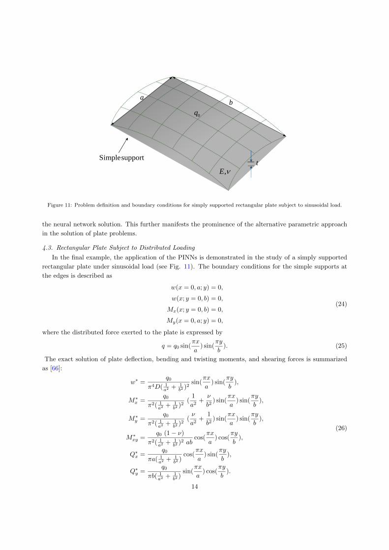
In the final example, the application of the PINNs is demonstrated in the study of a simply supported

rectangular plate under sinusoidal load (see Fig. 11). The boundary conditions for the simple supports at

the edges is described as

w(x = 0, a; y) = 0,

w(x; y = 0, b) = 0,

Mx(x; y = 0, b) = 0,

My(x = 0, a; y) = 0,

(24)

where the distributed force exerted to the plate is expressed by

q = q0 sin(πx

a) sin(

πy

b). (25)

The exact solution of plate deflection, bending and twisting moments, and shearing forces is summarized

as [66]:

w∗ =q0

π4D( 1a2 + 1

b2 )2sin(

πx

a) sin(

πy

b),

M∗x =q0

π2( 1a2 + 1

b2 )2(

1

a2+ν

b2) sin(

πx

a) sin(

πy

b),

M∗y =q0

π2( 1a2 + 1

b2 )2(ν

a2+

1

b2) sin(

πx

a) sin(

πy

b),

M∗xy =q0 (1− ν)

π2( 1a2 + 1

b2 )2 abcos(

πx

a) cos(

πy

b),

Q∗x =q0

πa( 1a2 + 1

b2 )cos(

πx

a) sin(

πy

b),

Q∗y =q0

πb( 1a2 + 1

b2 )sin(

πx

a) cos(

πy

b).

(26)

14

Here, a 200 cm × 300 cm rectangular plate with thickness t = 1 cm is considered, and is subject to a

sinusoidal load with intensity q0 = 0.01 kgf/cm2. The material properties of the plate are: Young’s modulus

of elasticity, E = 2.06× 106 kgf/cm2; Poisson’s ratio, ν = 0.25; and flexural rigidity, D = 183111 kgf.cm .

The solution variable set involves deflection, moments and forces, in Cartesian coordinates, i.e., w, Mx,

My, Mxy, Qx, Qy. These variables are defined as independent neural networks with the architecture of

choice

w(x, y) ' Nw(x, y),

Mx(x, y) ' NMx(x, y),

My(x, y) ' NMy (x, y),

Mxy(x, y) ' NMxy(x, y),

Qx(x, y) ' NQx(x, y),

Qy(x, y) ' NQy(x, y).

(27)

A network architecture of five layers with twenty neurons in each layer is used in this problem. The loss

function is expressed as

LΩ∗ = ‖w − w∗‖+ ‖Mx −M∗x‖+

∥∥My −M∗y∥∥+

∥∥Mxy −M∗xy∥∥

+ ‖Qx −Q∗x‖+∥∥Qy −Q∗y∥∥ ,

LΩ =

∥∥∥∥∂4w

∂x4+ 2

∂4w

∂x2 ∂y2+∂4w

∂y4− q∗

D

∥∥∥∥ ,L∂Ω =

∥∥∥∥Mx +D (∂2w

∂x2+ ν

∂2w

∂y2)

∥∥∥∥+

∥∥∥∥My +D (∂2w

∂y2+ ν

∂2w

∂x2)

∥∥∥∥+

∥∥∥∥Mxy −D (1− ν)∂2w

∂x∂y

∥∥∥∥ .

(28)

In the above relations, the asterisk denotes the given data related to the exact solution (i.e., Eq. (26)). In

contrast, the quantities without asterisk express the approximation functions of the neural network (i.e.,

Eq. (27)). Training is accomplished once the output values of all networks are as close as possible to the

given data. The cost function given by Eq. (28) can either be used for the solution of the plate deflection or

identification of the model parameters. For the case of parameter identification here, ν and D are treated

as unknown network parameters that are attainable by using the deep-learning-based solution. This task

can be easily carried out in SciANN with minimal coding (e.g., see [38]).

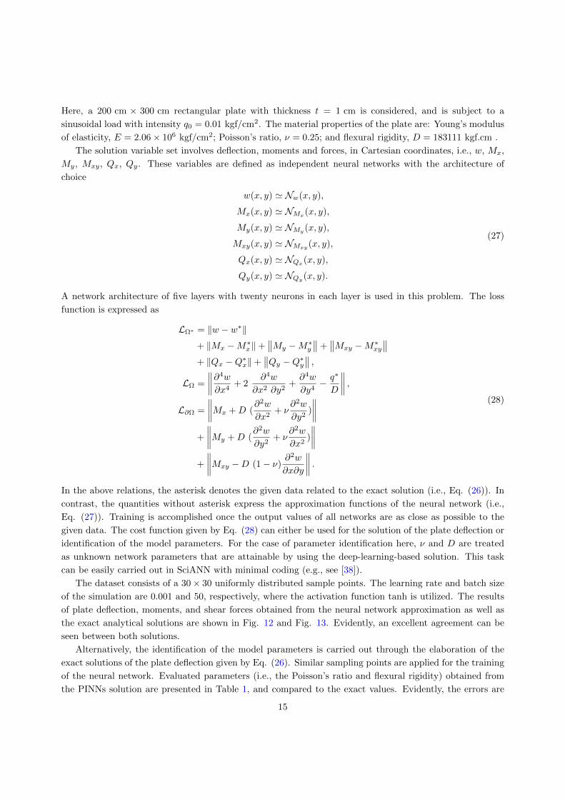
The dataset consists of a 30× 30 uniformly distributed sample points. The learning rate and batch size

of the simulation are 0.001 and 50, respectively, where the activation function tanh is utilized. The results

of plate deflection, moments, and shear forces obtained from the neural network approximation as well as

the exact analytical solutions are shown in Fig. 12 and Fig. 13. Evidently, an excellent agreement can be

seen between both solutions.

Alternatively, the identification of the model parameters is carried out through the elaboration of the

exact solutions of the plate deflection given by Eq. (26). Similar sampling points are applied for the training

of the neural network. Evaluated parameters (i.e., the Poisson’s ratio and flexural rigidity) obtained from

the PINNs solution are presented in Table 1, and compared to the exact values. Evidently, the errors are

15

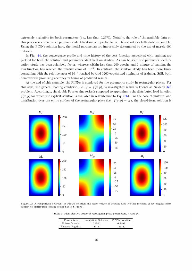
extremely negligible for both parameters (i.e., less than 0.25%). Notably, the role of the available data on

this process is crucial since parameter identification is in particular of interest with as little data as possible.

Using the PINNs solution here, the model parameters are impeccably determined by the use of merely 900

datasets.

In Fig. 14, the convergence profile and time history of the cost function associated with training are

plotted for both the solution and parameter identification studies. As can be seen, the parameter identifi-

cation study has been relatively faster, whereas within less than 200 epochs and 1 minute of training the

loss function has reached the relative error of 10−5. In contrast, the solution study has been more time-

consuming with the relative error of 10−4 reached beyond 1200 epochs and 4 minutes of training. Still, both

demonstrate promising accuracy in terms of predicted results.

At the end of this example, the PINNs is employed for the parametric study in rectangular plates. For

this sake, the general loading condition, i.e., q = f(x, y), is investigated which is known as Navier’s [69]

problem. Accordingly, the double Fourier sine series is supposed to approximate the distributed load function

f(x, y) for which the explicit solution is available in resemblance to Eq. (26). For the case of uniform load

distribution over the entire surface of the rectangular plate (i.e., f(x, y) = q0), the closed-form solution is

0

50

100

150

200

0

50

100

150

200

Mx

Mx* Mxy

* My*

Mxy My

- 75

- 50

- 25

0

25

50

75

- 75

- 50

- 25

0

25

50

75

0

20

40

60

80

100

120

0

20

40

60

80

100

120

Figure 12: A comparison between the PINNs solution and exact values of bending and twisting moment of rectangular platesubject to distributed loading (color bar in SI units).

Table 1: Identification study of rectangular plate parameters, ν and D.

Parameters Analytical Solution PINNs Solution

Poisson’s ratio 0.2500 0.2497Flexural Rigidity 183111 183382

16

described as [66]

w =16 q0

π6 D

k∑m=1

k∑n=1

sin mπxa sin nπy

b

mn (m2

a2 + n2

b2 )2, (29)

in which m and n are odd integers. Note all terms related to either case where m or n is an even number

vanish. It is noteworthy that the Fourier series lose their significance as m and/or n increase. Indeed, the

expansion related to n,m = 1, 3, 5 accommodates a near-exact solution accuracy (i.e., 99.9% precision [66])

to the plate deflection subject to uniform distributed loading q0, which follows

w =16 q0

π6 D(sin πx

a sin πyb

( 1a2 + 1

b2 )2+

sin πxa sin 3π y

b

3 ( 1a2 + 9

b2 )2+

sin πxa sin 5πy

b

5 ( 1a2 + 25

b2 )2+

sin 3πxa sin πy

b

3( 9a2 + 1

b2 )2+

sin 3πxa sin 3πy

b

9( 9a2 + 9

b2 )2+

sin 3πxa sin 5πy

b

15( 9a2 + 25

b2 )2+

sin 5πxa sin πy

b

5( 25a2 + 1

b2 )2+

sin 5πxa sin 3πy

b

15( 25a2 + 9

b2 )2+

sin 5πxa sin 5πy

b

25( 25a2 + 25

b2 )2).

(30)

In order to conduct the parametric study by means of PINNs, this solution is recast into the following format

300

200

100

0

- 100

- 200

- 300

300

200

100

0

- 100

- 200

- 300

Qx*

Qx

Qy*

Qy w

0

100

200

- 100

- 200

0

100

200

- 100

- 200

0.00

0.01

0.02

0.03

0.04

0.00

0.01

0.02

0.03

0.04

w*

Figure 13: A comparison between the PINNs solution and exact values of shearing forces and deflection of rectangular platesubject to distributed loading (color bar in SI units).

17

0 200 400 600 800 1,000 1,20010−5

10−4

10−3

10−2

10−1

100

Epochs

L/L0

0 60 120 180 240 30010−5

10−4

10−3

10−2

10−1

100

Time(s)

L/L0

Solution study

Identification study

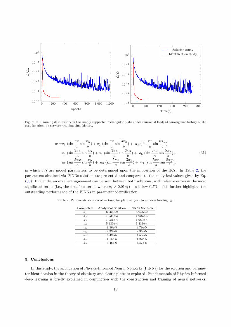
Figure 14: Training data history in the simply supported rectangular plate under sinusoidal load; a) convergence history of thecost function, b) network training time history.

w =a1 (sinπx

asin

πy

b) + a2 (sin

πx

asin

3πy

b) + a3 (sin

πx

asin

5πy

b)+

a4 (sin3πx

asin

πy

b) + a5 (sin

3πx

asin

3πy

b) + a6 (sin

3πx

asin

5πy

b)+

a7 (sin5πx

asin

πy

b) + a8 (sin

5πx

asin

3πy

b) + a9 (sin

5πx

asin

5πy

b),

(31)

in which ai’s are model parameters to be determined upon the imposition of the BCs. In Table 2, the

parameters obtained via PINNs solution are presented and compared to the analytical values given by Eq.

(30). Evidently, an excellent agreement can be seen between both solutions, with relative errors in the most

significant terms (i.e., the first four terms where ai > 0.01a1) lies below 0.5%. This further highlights the

outstanding performance of the PINNs in parameter identification.

Table 2: Parametric solution of rectangular plate subject to uniform loading, q0.

Parameters Analytical Solution PINNs Solution

a1 6.969e-2 6.944e-2a2 1.939e-3 1.927e-3a3 1.981e-4 1.989e-4a4 5.430e-4 5.433e-4a5 9.56e-5 9.79e-5a6 2.39e-5 2.31e-5a7 4.49e-5 4.55e-5a8 1.15e-5 1.22e-5a9 4.46e-6 3.57e-6

5. Conclusions

In this study, the application of Physics-Informed Neural Networks (PINNs) for the solution and parame-

ter identification in the theory of elasticity and elastic plates is explored. Fundamentals of Physics-Informed

deep learning is briefly explained in conjunction with the construction and training of neural networks.

18

Thereafter, the application of PINNs to the theory of elasticity is studied. The Airy stress function and the

biharmonic PDEs governing the elasticity solutions are presented in the general form. The application of

PINNs in the solution of the Lame Problem is demonstrated, as a representative benchmark example involv-

ing a simplified biharmonic ODE formulation in polar coordinates. In addition, an Airy-inspired parametric

solution to the same problem is investigated, which is developed by a manufactured combination of a set

of nonlinear terms based on the theory of elasticity. It is shown that Airy-network results in superior con-

vergence and accuracy characteristics. The next example is dedicated to the foundation problem, in which

the PINNs solution of a simplified PDE in polar coordinates is developed in conjunction with mapping in

Cartesian coordinates. It is shown the alternative use of Airy-inspired neural networks outperforms the

classic PINNs solution by a fair margin. The application of PINNs for solution and discovery in the theory

of elastic plates is implemented next. The fourth-order PDE governing the lateral deflection of thin plates is

explained concisely. A circular plate under concentrated loading is studied, which involves the application

of PINNs to the solution of reduced third order ODE of plate deflection in polar coordinates. The manufac-

tured solution inspired by the analytical approach is exercised and proven to be a promising alternative to

the general PINN approach again. The final example is devoted to a rectangular plate subject to distributed

loading. This example consists of both the solution and parameter identification of the generic fourth-order

PDE of plate deflection. As a remedy, Fourier series are elaborated to investigate the solution of plates

deflection, which demonstrates enormous improvement in terms of training duration and accuracy. In this

fashion, it is shown that the classical analytical methods could contribute significantly to the construction

of neural networks with a minimal number of parameters that are very accurate and fast to evaluate. Thus,

they can be used to guide the construction of more efficient physics-informed neural networks. Considering

that Fourier features are now commonly employed to construct more trainable neural networks, a natural

extension would be to also add Airy features to improve the trainability of neural networks for problems of

continuum mechanics.

Data Availability Statement

All data, models, or source codes that support the findings of this study are available from the corre-

sponding author upon reasonable request.

References

[1] A. Graves, A.-r. Mohamed, G. Hinton, Speech recognition with deep recurrent neural networks, in: 2013 IEEE internationalconference on acoustics, speech and signal processing, Ieee, pp. 6645–6649.

[2] T.-H. Chan, K. Jia, S. Gao, J. Lu, Z. Zeng, Y. Ma, Pcanet: A simple deep learning baseline for image classification, IEEEtransactions on image processing 24 (2015) 5017–5032.

[3] M. I. Razzak, S. Naz, A. Zaib, Deep learning for medical image processing: Overview, challenges and the future, Classi-fication in BioApps (2018) 323–350.

[4] M. Reichstein, G. Camps-Valls, B. Stevens, M. Jung, J. Denzler, N. Carvalhais, et al., Deep learning and processunderstanding for data-driven earth system science, Nature 566 (2019) 195–204.

[5] G. Pilania, C. Wang, X. Jiang, S. Rajasekaran, R. Ramprasad, Accelerating materials property predictions using machinelearning, Scientific reports 3 (2013) 1–6.

[6] K. J. Bergen, P. A. Johnson, V. Maarten, G. C. Beroza, Machine learning for data-driven discovery in solid earthgeoscience, Science 363 (2019).

[7] Z. Shi, E. Tsymbalov, M. Dao, S. Suresh, A. Shapeev, J. Li, Deep elastic strain engineering of bandgap through machinelearning, Proceedings of the National Academy of Sciences 116 (2019) 4117–4122.

[8] M. Brenner, J. Eldredge, J. Freund, Perspective on machine learning for advancing fluid mechanics, Physical ReviewFluids 4 (2019) 100501.

[9] H. Wu, A. Mardt, L. Pasquali, F. Noe, Deep generative markov state models, arXiv preprint arXiv:1805.07601 (2018).[10] Q. Zhu, Z. Liu, J. Yan, Machine learning for metal additive manufacturing: predicting temperature and melt pool fluid

dynamics using physics-informed neural networks, Computational Mechanics 67 (2021) 619–635.

19

[11] S. Im, H. Kim, W. Kim, M. Cho, Neural network constitutive model for crystal structures, Computational Mechanics 67(2021) 185–206.

[12] C. Anitescu, E. Atroshchenko, N. Alajlan, T. Rabczuk, Artificial neural network methods for the solution of second orderboundary value problems, Computers, Materials and Continua 59 (2019) 345–359.

[13] S. Bhatnagar, Y. Afshar, S. Pan, K. Duraisamy, S. Kaushik, Prediction of aerodynamic flow fields using convolutionalneural networks, Computational Mechanics 64 (2019) 525–545.

[14] Y. Yang, P. Perdikaris, Conditional deep surrogate models for stochastic, high-dimensional, and multi-fidelity systems,Computational Mechanics 64 (2019) 417–434.

[15] V. Minh Nguyen-Thanh, L. Trong Khiem Nguyen, T. Rabczuk, X. Zhuang, A surrogate model for computational homog-enization of elastostatics at finite strain using high-dimensional model representation-based neural network, InternationalJournal for Numerical Methods in Engineering 121 (2020) 4811–4842.

[16] D. P. Boso, D. Di Mascolo, R. Santagiuliana, P. Decuzzi, B. A. Schrefler, Drug delivery: Experiments, mathematicalmodelling and machine learning, Computers in Biology and Medicine 123 (2020) 103820.

[17] M. Lefik, D. Boso, B. Schrefler, Artificial neural networks in numerical modelling of composites, Computer Methods inApplied Mechanics and Engineering 198 (2009) 1785–1804.

[18] D. Zhang, J. Lin, Q. Peng, D. Wang, T. Yang, S. Sorooshian, X. Liu, J. Zhuang, Modeling and simulating of reservoiroperation using the artificial neural network, support vector regression, deep learning algorithm, Journal of Hydrology565 (2018) 720–736.

[19] S. Bouktif, A. Fiaz, A. Ouni, M. A. Serhani, Optimal deep learning lstm model for electric load forecasting using featureselection and genetic algorithm: Comparison with machine learning approaches, Energies 11 (2018) 1636.

[20] A. Mayr, G. Klambauer, T. Unterthiner, S. Hochreiter, Deeptox: toxicity prediction using deep learning, Frontiers inEnvironmental Science 3 (2016) 80.

[21] H. Dehghani, A. Zilian, Ann-aided incremental multiscale-remodelling-based finite strain poroelasticity, ComputationalMechanics (2021) 1–24.

[22] X. Lu, D. G. Giovanis, J. Yvonnet, V. Papadopoulos, F. Detrez, J. Bai, A data-driven computational homogenizationmethod based on neural networks for the nonlinear anisotropic electrical response of graphene/polymer nanocomposites,Computational Mechanics 64 (2019) 307–321.

[23] M. Raissi, H. Babaee, G. E. Karniadakis, Parametric gaussian process regression for big data, Computational Mechanics64 (2019) 409–416.

[24] B. Bahmani, W. Sun, A kd-tree-accelerated hybrid data-driven/model-based approach for poroelasticity problems withmulti-fidelity multi-physics data, Computer Methods in Applied Mechanics and Engineering 382 (2021) 113868.

[25] A. Deshpande, C. Guestrin, S. R. Madden, J. M. Hellerstein, W. Hong, Model-driven data acquisition in sensor networks,in: Proceedings of the Thirtieth international conference on Very large data bases-Volume 30, pp. 588–599.

[26] H. Owhadi, Bayesian numerical homogenization, Multiscale Modeling & Simulation 13 (2015) 812–828.[27] J. Han, A. Jentzen, E. Weinan, Solving high-dimensional partial differential equations using deep learning, Proceedings

of the National Academy of Sciences 115 (2018) 8505–8510.[28] Y. Bar-Sinai, S. Hoyer, J. Hickey, M. P. Brenner, Learning data-driven discretizations for partial differential equations,

Proceedings of the National Academy of Sciences 116 (2019) 15344–15349.[29] S. H. Rudy, S. L. Brunton, J. L. Proctor, J. N. Kutz, Data-driven discovery of partial differential equations, Science

Advances 3 (2017) e1602614.[30] M. Raissi, P. Perdikaris, G. E. Karniadakis, Physics-informed neural networks: A deep learning framework for solving

forward and inverse problems involving nonlinear partial differential equations, Journal of Computational Physics 378(2019) 686–707.

[31] A. G. Baydin, B. A. Pearlmutter, A. A. Radul, J. M. Siskind, Automatic differentiation in machine learning: a survey,Journal of machine learning research 18 (2018).

[32] M. Abadi, P. Barham, J. Chen, Z. Chen, A. Davis, J. Dean, M. Devin, S. Ghemawat, G. Irving, M. Isard, et al.,Tensorflow: A system for large-scale machine learning, in: 12th USENIX symposium on operating systems design andimplementation (OSDI 16), pp. 265–283.

[33] F. Chollet, et al., keras, 2015.[34] E. Haghighat, R. Juanes, Sciann: A keras/tensorflow wrapper for scientific computations and physics-informed deep

learning using artificial neural networks, Computer Methods in Applied Mechanics and Engineering 373 (2021) 113552.[35] Z. Mao, A. D. Jagtap, G. E. Karniadakis, Physics-informed neural networks for high-speed flows, Computer Methods in

Applied Mechanics and Engineering 360 (2020) 112789.[36] F. Sahli Costabal, Y. Yang, P. Perdikaris, D. E. Hurtado, E. Kuhl, Physics-informed neural networks for cardiac activation

mapping, Frontiers in Physics 8 (2020) 42.[37] E. Kharazmi, Z. Zhang, G. E. Karniadakis, hp-vpinns: Variational physics-informed neural networks with domain decom-

position, Computer Methods in Applied Mechanics and Engineering 374 (2021) 113547.[38] E. Haghighat, M. Raissi, A. Moure, H. Gomez, R. Juanes, A deep learning framework for solution and discovery in solid

mechanics, arXiv preprint arXiv:2003.02751 (2020).[39] E. Haghighat, A. C. Bekar, E. Madenci, R. Juanes, A nonlocal physics-informed deep learning framework using the

peridynamic differential operator, arXiv preprint arXiv:2006.00446 (2020).[40] M. Guo, E. Haghighat, An energy-based error bound of physics-informed neural network solutions in elasticity, arXiv

preprint arXiv:2010.09088 (2020).[41] L. Zhang, L. Cheng, H. Li, J. Gao, C. Yu, R. Domel, Y. Yang, S. Tang, W. K. Liu, Hierarchical deep-learning neural

networks: finite elements and beyond, Computational Mechanics 67 (2021) 207–230.

20

[42] X. Yang, S. Zafar, J.-X. Wang, H. Xiao, Predictive large-eddy-simulation wall modeling via physics-informed neuralnetworks, Physical Review Fluids 4 (2019) 034602.

[43] Y. Yang, P. Perdikaris, Adversarial uncertainty quantification in physics-informed neural networks, Journal of Computa-tional Physics 394 (2019) 136–152.

[44] Q. He, D. Barajas-Solano, G. Tartakovsky, A. M. Tartakovsky, Physics-informed neural networks for multiphysics dataassimilation with application to subsurface transport, Advances in Water Resources 141 (2020) 103610.

[45] Q. Lou, X. Meng, G. E. Karniadakis, Physics-informed neural networks for solving forward and inverse flow problems viathe boltzmann-bgk formulation, arXiv preprint arXiv:2010.09147 (2020).

[46] C. Rao, H. Sun, Y. Liu, Physics-informed deep learning for computational elastodynamics without labeled data, Journalof Engineering Mechanics 147 (2021) 04021043.

[47] S. Cai, Z. Wang, S. Wang, P. Perdikaris, G. E. Karniadakis, Physics-informed neural networks for heat transfer problems,Journal of Heat Transfer 143 (2021) 060801.

[48] U. b. Waheed, E. Haghighat, T. Alkhalifah, C. Song, Q. Hao, Pinneik: Eikonal solution using physics-informed neuralnetworks, Computers and Geosciences 155 (2021) 104833.

[49] G. E. Karniadakis, I. G. Kevrekidis, L. Lu, P. Perdikaris, S. Wang, L. Yang, Physics-informed machine learning, NatureReviews Physics 3 (2021) 422–440.

[50] M. A. Hearst, S. T. Dumais, E. Osuna, J. Platt, B. Scholkopf, Support vector machines, IEEE Intelligent Systems andtheir applications 13 (1998) 18–28.

[51] C. K. Williams, C. E. Rasmussen, Gaussian processes for machine learning, volume 2, MIT press Cambridge, MA, 2006.[52] D. Svozil, V. Kvasnicka, J. Pospichal, Introduction to multi-layer feed-forward neural networks, Chemometrics and

intelligent laboratory systems 39 (1997) 43–62.[53] J. Gu, Z. Wang, J. Kuen, L. Ma, A. Shahroudy, B. Shuai, T. Liu, X. Wang, G. Wang, J. Cai, et al., Recent advances in

convolutional neural networks, Pattern Recognition 77 (2018) 354–377.[54] L. R. Medsker, L. Jain, Recurrent neural networks, Design and Applications 5 (2001).[55] D. P. Kingma, J. Ba, Adam: A method for stochastic optimization, arXiv preprint arXiv:1412.6980 (2014).[56] G. B. Airy, On the strains in the interior of beams, Report of the British Association for the Advancement of Science 32

(1862) 82–86.[57] J. C. Maxwell, The Scientific Papers of James Clerk Maxwell, volume 2, University Press, 1890.[58] S. P. Timoshenko, J. Goodier, Theory of elasticity, McGraw-hill, 1951.[59] A. P. Boresi, K. Chong, J. D. Lee, Elasticity in engineering mechanics, John Wiley & Sons, 2010.[60] A. A. Katebi, A. Khojasteh, M. Rahimian, R. Y. Pak, Axisymmetric interaction of a rigid disc with a transversely isotropic

half-space, International journal for numerical and analytical methods in geomechanics 34 (2010) 1211–1236.[61] G. Lame, Lessons on the mathematical theory of the elasticity of solid bodies, Bachelier, Paris (1852).[62] P. Virtanen, R. Gommers, T. E. Oliphant, M. Haberland, T. Reddy, D. Cournapeau, E. Burovski, P. Peterson,

W. Weckesser, J. Bright, et al., Scipy 1.0: fundamental algorithms for scientific computing in python, Nature meth-ods 17 (2020) 261–272.

[63] S. Timoshenko, History of strength of materials: with a brief account of the history of theory of elasticity and theory ofstructures, Courier Corporation, 1983.

[64] G. Kirchhoff, Uber das Gleichgewicht und die Bewegung einer elastischen Scheibe, 1850.[65] A. E. H. Love, XVI. the small free vibrations and deformation of a thin elastic shell, Philosophical Transactions of the

Royal Society of London.(A.) (1888) 491–546.[66] S. P. Timoshenko, S. Woinowsky-Krieger, Theory of plates and shells, McGraw-hill, 1959.[67] J. N. Reddy, Theory and analysis of elastic plates and shells, CRC press, 2006.[68] P. Kelly, Solid mechanics part ii: Engineering solid mechanicssmall strain, The University of Auckland (2013).[69] C. L. M. N. Navier, Extrait des recherche sur la flexion des planes elastiques, Bulletin des science de la societe philomartique

de Paris 5 (1823) 95–102.

21