Computer Physics Communications

Computer Physics Communications 104 (1997) 1-14

Artificial neural network methods in quantum mechanics I.E. Lagaris ‘, A. Likas, D.I. Fotiadis

Department of Computer Science, University of loannina, PO. Box 1186, CR 45110 loannina, Greece

Received 17 March 1997; revised 22 April 1997

Abstract

In a previous article we have shown how one can employ Artificial Neural Networks (ANNs) in order to solve non-homogeneous ordinary and partial differential equations. In the present work we consider the solution of eigenvalue problems for differential and integrodifferential operators, using ANNs. We start by considering the Schrodinger equation for the Morse potential that has an analytically known solution, to test the accuracy of the method. We then proceed with the Schr6dinger and the Dirac equations for a muonic atom, as well as with a nonlocal Schrijdinger integrodifferential equation that models the n + a system in the framework of the resonating group method. In two dimensions we consider the well-studied Henon-Heiles Hamiltonian and in three dimensions the model problem of three coupled anharmonic oscillators. The method in all of the treated cases proved to be highly accurate, robust and efficient. Hence it is a promising tool for tackling problems of higher complexity and dimensionality. @ 1997 Elsevier Science B.V.

PACS: 02.6O.Lj; 02.60.Nm; 02.70.Jn; 03.65.Ge Keywords: Neural networks; Eigenvatue problems; Schrodinger; Dirac; Collocation; Optimization

1. Introduction

In a previous work [l] a general method has been presented for solving both ordinary differential equations (ODES) and partial differential equations (PDEs) . This method relies on the function approximation capabilities of feedforward neural networks and leads to the construction of a solution written in a differentiable, closed analytic form. The trial solution is suitably written so as to satisfy the appropriate initial/boundary conditions and employs a feedforward neural network as the main approximation element. The parameters of the network (weights and biases) are then adjusted so as to minimize a suitable error function, which in turn is equivalent to satisfying the differential equation at selected points in the definition domain.

There are many results both theoretical and experimental that testify for the approximation capabilities of neural networks [ 3-51. The most important one is that a feedforward neural network with one hidden layer can approximate any function to arbitrary accuracy by appropriately increasing the number of units in the hidden layer [4]. This fact has led us to consider this type of network architecture as a candidate model for treating

’ E-mail:lagaris@cs.uoi.gr

OOlO-4655/97/$17.00 @ 1997 Elsevier Science B.V. All rights reserved. PllSOOlO-4655(97)00054-4

2 LE. Lagaris et ul./Computer Physics Communications 104 (1997) I-14

differential equations. In fact, the employment of neural networks as a tool for solving differential equations has many attractive features [ I] : l The solution via neural networks is a differentiable, closed analytic form easily used in any subsequent

calculation with superior interpolation capabilities. l Compact solution models are obtained due to the small number of required parameters. This fact also results

in low memory demands. l There is the possibility of direct hardware implementation of the method on specialized VLSI chips called

neuroprocessors. In such a case there will be a tremendous increase in the processing speed that will offer the opportunity to tackle many difficult high-dimensional problems requiring a large number of grid points. Alternatively, it is also possible for the proposed method to be efficiently implemented on parallel architectures. In this paper we present a novel technique for solving eigenvalue problems of differential and integrodifferen-

tial operators in one, two and three dimensions, that is based on the use of MLPs for the parametrization of the solution, on the collocation method for the formulation of the error function and on optimization procedures.

All the problems we tackle come from the field of Quantum Mechanics, i.e. we solve mainly Schriidinger problems and we have applied the same technique to the Dirac equation that is reduced to a system of coupled ODES. In addition, for the Schriidinger equation one can employ the Raleigh-Ritz variational principle, where again the variational trial wavefunction is parametrized using MLPs. For the two-dimensional Hennon-Heiles potential [ 21, we compare the resulting variational and the collocation solutions.

A description of the general formulation of the proposed approach is presented in Section 2. Section 3 illustrates several cases of problems where the proposed technique has been applied along with details concerning the implementation of the method and the accuracy of the obtained solution. In addition, in a two-dimensional problem, we provide a comparison of our results with those obtained by a solution based on finite elements. Finally, Section 4 contains conclusions and directions for future research.

2. The method

Consider the following differential equation:

HP(r) = f(r), in D, (1)

W(r) =O, on aD, (2)

where H is a linear differential operator, f(r) is a known function, D C R3 and c?D is the boundary of D. Moreover, we denote D = D U JD. We assume that f E C(D) and the solution p(r) belongs to Ck(n), the space of continuous functions with continuous partial derivatives up to k order inclusive (k is the higher order derivative appearing in the operator H, HP(r) E C(D) ) . The set of the admissible functions

{P(r) E cm, r E D c R3, P(r) =0 on JD}

forms a linear space. In the present analysis we also assume that the domain under consideration D is bounded and its boundary dD is sufficiently smooth (Lipschitzian) .

In order to solve this problem we have proposed a technique [ l] that considers a trial solution of the form pt;( r) = A(r) + B( r, A) N( r, p) which employs a feedforward neural network with parameter vector p (to be adjusted). The parameter vector h should also be adjusted during minimization. The specification of functions A and B should be done so that p, satisfies the boundary conditions regardless of the values of p and A.

To obtain a solution to the above differential equation, the collocation method has been employed [6] which assumes a discretization of the domain D into a set points ri. The problem is then transformed into a minimization one with respect to the parameter vectors p and A,

I.E. Lagaris et al./Compupurer Physics Communicutiuns 104 (1997) I-14 3

min PA c [H*t(ri) - f(ri) I*. (3)

i

If the obtained minimum has a value close to zero, then we consider that an approximate solution has been recovered.

Consider now the case of the following general eigenvalue problem:

HP(r) = @P(r), in D, (4)

W(r) =O, on iID. (5)

In this case a trial solution may take the form p,(r) = B(r, A)N(r,p), where B(r, h) is zero on dD, for a range of values of A. By discretizing the domain, the problem is transformed to minimizing the following error quantity, with respect to the parameters p and A:

Enor(p ,

Al = Ci[Hpf(ri9P9h) -EWt(ri,PYA)12 .wt12dr ’

where E is computed as

(7)

A method similar in spirit has been proposed long ago by Frost et al. [7] and is known as the “Local Energy Method”. In the proposed approach the trial solution pt employs a feedforward neural network and more specifically a multilayer perceptron (MLP) . The parameter vector p corresponds to the weights and biases of the neural architecture. Although it is possible for the MLP to have many hidden layers we have considered here the simple case of single hidden layer MLPs, which have been proved adequate for our test problems.

Consider a multilayer perceptron with n input units, one hidden layer with m sigmoid units and a linear output unit (Fig. 1) . The extension to the case of more than one hidden layers can be obtained accordingly. For a given input vector r = (II,. _ , r,) the output of the network is N = CE, Uia( zi), where zi = cy=i Wijrj + Ui, wij denotes the weight from the input unit j to the hidden unit i, Ui the weight from the hidden unit i to the output, Ui the bias of hidden unit i and V(Z) the sigmoid transfer function: (T(Z) = l/( 1 + exp( -z)). It is straightforward to show that [ l]

where ci = u(zi) and u(k) denotes the kth order derivative of the sigmoid. Moreover, it is readily verifiable that

(9)

where ”

and A = Cy,i Ai. Once the derivative of the error with respect to the network parameters has been defined, it is then straight-

forward to employ almost any minimization technique. For example it is possible to use either the steepest

I.E. Lagaris et al./Computer Physics Communications 104 (1997) I-14

Input Layer Hidden

I ,aver

Fig. 1. Feedforward neural network with one hidden layer.

descent (i.e., the backpropagation algorithm or any of its variants), or the conjugate gradient method or other techniques proposed in the literature. We used the MERLIN optimization package [8,9] for our experiments, where many algorithms are available. We mention in passing that the BFGS method has demonstrated outstand- ing performance. Note that for a given grid point the calculation of the gradient of each network with respect to the adjustable parameters lends itself to parallel computation.

Using the above approach it is possible to calculate any number of states. This is done by projecting out from the trial wavefunction the already computed levels.

IfI~o)o),l~l),... , IPk) are computed orthonormal states, a trial state ]?P,) orthogonal to all of them can be obtained by projecting out their components from a general function I!@,) that respects the boundary conditions, namely

3. Examples

3.1. Schriidinger equation for the Morse Potential

The Morse Hamiltonian for the Zz-molecule in the atomic units system is given by

H = -f -$ + V(x) ) P

where V(x) = D [ e-2ax - 2eeax + 1 ] and D = 0.0224, CY = 0.9374, ,X = 119406. The energy levels are known analytically [ 131, and are given by E,, = (n + i) ( 1 - (n + $)/c)&, with

5 = 156.047612535 and 5 = 5.741837286 x 10P4. The ground state energy is l a = 0.286171979 x 10d3. We parametrize as

cf+(x) = e -PxZN(X,U,W,V), p > 0,

with N being a feedforward artificial neural network with one hidden layer and m sigmoid hidden units, i.e.

j=l

I.E. Lagaris et al./Computer Physics Communications 104 (1997) I-14 5

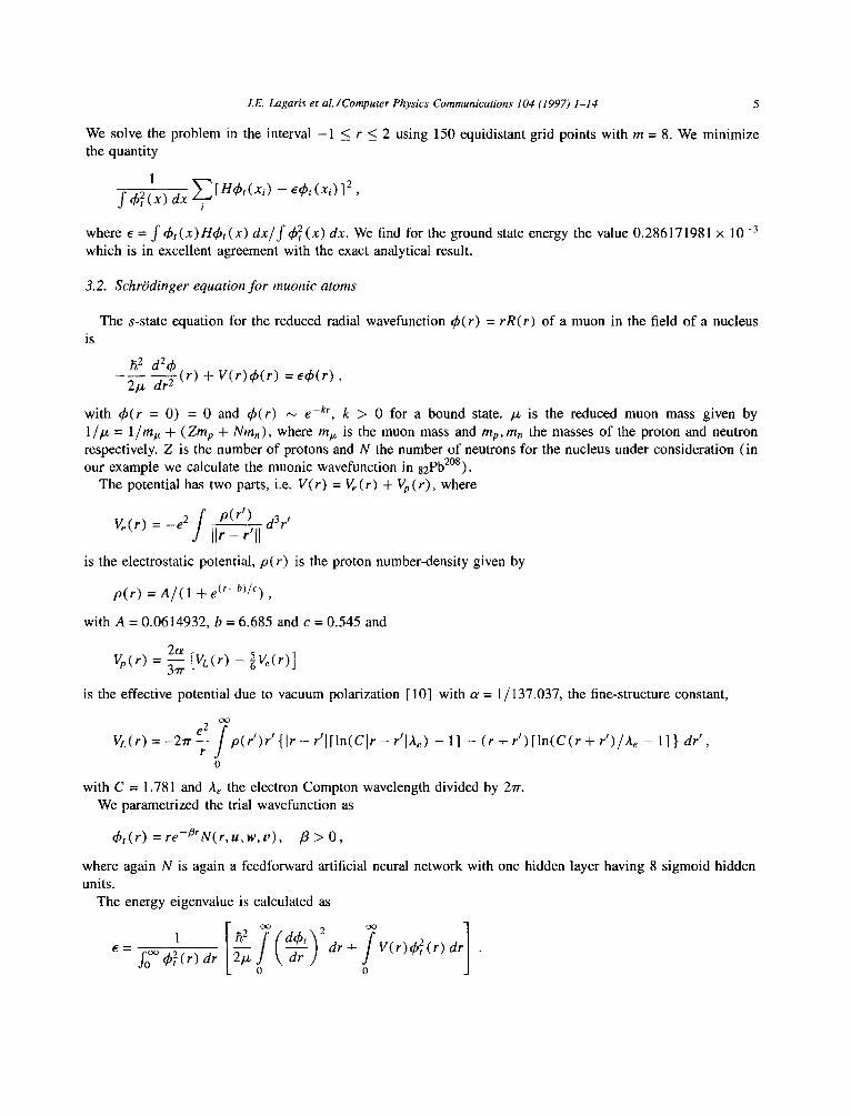
We solve the problem in the interval -1 < r 5 2 using 150 equidistant grid points with m = 8. We minimize the quantity

Id?:x)dx~ [Wt(Xi) - EMXi)12,

where E = J #+(x)H&(x) &/J&(x) dx. We find for the ground state energy the value 0.286171981 x 10e3 which is in excellent agreement with the exact analytical result.

3.2. Schriidinger equation for muonic atoms

The s-state equation for the reduced radial wavefunction 4(r) = rR( r) of a muon in the field of a nucleus is

with 4(r = 0) = 0 and 4(r) N epkr, k > 0 for a bound state. p is the reduced muon mass given by 1 /,u = l/m, + (Zm, + Nm,), where mp is the muon mass and mp, m, the masses of the proton and neutron respectively. Z is the number of protons and N the number of neutrons for the nucleus under consideration (in our example we calculate the muonic wavefunction in s2Pb2’*).

The potential has two parts, i.e. V(r) = V,(r) + V,(r), where

V,(r) = -e2 s

,,r”:,,, d3r’

is the electrostatic potential, p(r) is the proton number-density given by

p(r) = A/( 1 + e(r-b)‘c) ,

with A = 0.0614932, b = 6.685 and c = 0.545 and

is the effective potential due to vacuum polarization [ lo] with cy = l/137.037, the fine-structure constant,

Q(r)=-27rfjp(r’)r’{ir-r’i[ln(C/r-r’jl,) -11 - (r+r’)[ln(C(r+r’)/A, - 11) dr’, 0

with C = 1.781 and A, the electron Compton wavelength divided by 27r. We parametrized the trial wavefunction as

+f(r) = re-@‘N(r,u,w,u), /I > 0,

where again N is again a feedforward artificial neural network with one hidden layer having 8 sigmoid hidden units.

The energy eigenvalue is calculated as

e= Jr$(r)dr [~[(~~dr+~V(r)&(r)dr] .

I.E. Laguris et al. /Computer Physics Communicutions IO4 (1997) I-14

-0.07 - /

-0.06 .r - .i'

:; :',' -0.09

-y -

-0.1 _. 0 0 5 5 10 10 15 15 20 20 25 25 30 30 35 35 40 40

Fig. 2. Ground state of (a),(b) the Dirac and (c) the Schrijdinger equation for muonic atoms. Fig. 2. Ground state of (a),(b) the Dirac and (c) the Schrijdinger equation for muonic atoms.

have been calculated using the Gauss-Legendre rule. We used 80 points in the range have been calculated using the Gauss-Legendre rule. We used 80 points in the range The integrals quantity

[0,40]. The

is being minimized with respect to IL, w, U. We used for pi the same points as in the Gauss-Legendre Integration. We obtained for the energy E =

- 10.47 MeV. The radial wavefunction C#I( r) /r is shown in Fig. 2c.

3.3. Dirac equation for muonic atoms

The relativistic Dirac s-state equations for the small and large parts of the reduced radial wavefunction of a muon bound by a nucleus are [ 1 I]

with ,u and V(r) being as in the previous example. The total energy E is calculated by

m

V(r)b?(r)-f2(r)ldr .

We parametrized the trial solutions f,(r) and gt( r) as

fdr) =re +‘N(r,uf,Wf,vf), P > 0,

g,(r) = reCp’ N(r,u,,w,,u,), P > 0,

I.E. Lqaris et al./Compurer- Physics Conznzunications 104 (1997) l-14

and minimized the following error quantity:

-yi{ [ Ly + Ly - d-yrl) g(ri)]2 + [ 4y - ky _ Pc2+yl) fcr,)]2}

.l,“[g*tr) + f2(r>l dr

The binding energy is given by E = E - ,uc 2. We find E = -10.536 MeV. The small and the large parts of the radial wavefunction f( T)/Y and g(r)/r are shown in Fig. 2a and 2b, along with the Schriidinger radial wavefunction (Fig. 2~). The integrals and the training were performed using the same points as in the previous example.

3.4. Non-local Schriidinger equation for the n + a system

We consider here the nonlocal Schrijdinger equation

co

t; s(r) + V(r)+,(r) + /Ko(r,r’)4(r’) dr’ = e+(r) , --

0

with V(r) = -VOe-Pr2, where Vo = 41.28386, j? = 0.2751965 and i&( r, r’) = -Ae-y(r2+r”)(e2krr’ - e-2krr’) with A = -62.03772 , y = -0.8025, k = 0.46. This describes the n + LY system and is derived in the framework of the Resonating Group Method [ 121, /A is the system’s reduced mass given by 1 /,u = 1 /m, + l/ ( 2m, + 2m,).

We parametrized the trial wavefunction as

q&(r) = re-@N(r,u,w,v), p > 0,

where the neural architecture is the same as in the previous cases and minimized the following error quantity:

Ci {-J$ $&(ri) + V(ri)+,(ri) + sp Ko(ri,r’)$,(r’) dr’ - E&(ri)}*

~,“&tr) dr

where the energy is estimated by

E= ~S,“t~)2dr+SoOOV(r)~:(r)dr+S,“S,”OKotr,r’)~,tr)~,(r’)drdr’ s,“&(r) dr

We have considered 100 equidistant points in [ 0, 121 and the computed ground state is depicted in Fig. 3, while the corresponding eigenvalue was found equal to -24.07644, in agreement with previous calculations [ 21.

3.5. Two-dimensional Schriidinger equation

We consider here the well-studied [2] example of the Henon-Heiles potential. The Hamiltonian is written as

H=-; ($+$) +V(x,y),

with V(n,y) = i(x* +y*) + &(xy2 - i..$). We parametrize the trial solution as

I.E. Lagaris et al./Computer Physics Communicarions 104 (1997) I-14

0.6

0.5

0.4

0.3

0.2

0.1

0 0 2 4 6 a 10 12

Fig. 3. Ground state of the nonlocal SchrCidinger equation for the n + a system (e = -24.07644).

h(-LY) =e- *(xZ+y2)N(X, y, u, w(x), w(y), U)) A>O,

where N is a feedforward neural network with one hidden layer (with m = 8 sigmoid hidden units) and two input nodes (accepting the x and y values),

N(x, ~9 U, w(‘), w(‘), U) = 2 u,~cT(xw~‘) f J’Wj’) + Uj) . j=l

We have considered a grid of 20 x 20 points in [ -6,6] x [ -6,6]. The quantity minimized is

C,j[H$,(xivYj) -E4h(Xi~Yj)l 2

J_“,.f?“~XdY&(X,Y) ’ (11)

where the energy is calculated by

For this problem we calculate not only the ground state but a few more levels. The way we followed is the extraction from the trial wavefunction of the already computed levels as described in Section 2. If for example by C#JO ( X, y) we denote the normalized ground state, the trial wavefunction to be used for the computation of another level would be

where 4, (x, y) is parametrized in the same way as before. Note that +J, (x, y) is orthogonal to &0(x, y) by construction. Following this procedure we calculated the

first four levels for the Henon-Heiles Hamiltonian. Our results are reported in Figs. 4-7.

I.E. Lugaris et al./Cotnputer Physics Communications 104 (1997) I-14 9

0.6 0.5

0.5 0.4 0.3

0.4 0.2

0.3 0.1

0

0.2 -0.1 -0.2

0.1 -0.3 -0.4

0 -0.5

Fig. 4. Fig. 5.

Fig. 4. Ground state of the Henon-Heiles problem (E = 0.99866)

Fig. 5. First excited state of the Henon-Heiles problem (6 = 1.990107)

Fig. 6. Fig. 7

Fig. 6. Second excited state (degenerate) of the Henon-Heiles problem (E = 1.990107).

Fig. 7. Third excited state of the Henon-Heiles problem (E = 2.957225)

We also calculated the variational ground state wave-function for this problem by minimizing the expectation value of the Hamiltonian, using an identical neural form. In Figs. 8, 9, we plot the pointwise error, i.e. the (normalized) summand of I$. ( 11) for the collocation and the variational wavefunctions, respectively.

3.6. Three coupled anharmonic oscillators

As a three-dimensional example we consider the potential for the three coupled sextic anharmonic oscilla- tors [18],

V(x,y,z)=V(x)+Vty)+V(z)+xy+xz+yz,

where

V(x) = $2 + 2x4 + &x6.

The trial solution r$r ( X, y. z ) is parametrized as

r$r(x,y,z) = e-h(X*+v2+z2)N(x,y,z,u,W(*),W(y),~(Z),~), A > 0,

I.E. Lagaris et al. /Computer Physics Communications IO4 (1997) I-14

Fig. 8. Fig. 9

Fig. 8. Pointwise normalized error for the collocation wavefunction.

Fig. 9. Pointwise normalized error for the variational wavefunction.

where N is a feedforward neural network with one hidden layer (with m = 25 hidden units) and three input nodes (accepting the values of x, y and z),

N(X, Y, Z, U, Wcx), IV(‘), IV(‘)* U) = 2 UjCT(XWj’) + YW~“’ + ZWj’) + Uj) . j=l

We have considered a 28x28~28 grid in the [ -4,4] x [ -4,4] x [ -4,4] domain both for computing the integrals and calculating the following error quantity that was minimized:

Ci,j,k[H4t(Xi9YjJk) -E4t(Xi~Yj~Zk)12

s_“,s_“,s_“,~:(x,Y,z)dxdYdz ’

where the energy is calculated by

E= ~~~~_q$~~~~t(x~~~z)H~t(x,y,z)dxdydz ./-?./:mf~&(~,~,z) dxdydz ’

The ground state was computed and the corresponding eigenvalue was found equal to 2.9783, in agreement with the highly accurate result obtained by Kaluza [ 181.

4. Finite element approach

The two-dimensional Schrondiger equation for the Henon-Heiles potential was also solved using the finite element approach in which the solution is expressed in terms of piecewise continuous biquadratic basis functions,

(I/ = C @i@i(S9 n> , (12) i=l

where @i is the biquadratic basis function and +i is the unknown at the ith node of the element. The physical domain (x, y) is mapped on the computational domain (5, n) through the isoparametric mapping

x= c Xi@i(<v n) 9 (13) i=l

I.E. Laguris ei d/Computer Physics Communications 104 (1997) 1-14 11

Y =CYi@i(5,n) 7 (14) i=l

where 5 and n are the local coordinates in the computational domain (0 5 5, n < 1) and xi, yi the ith node coordinates in the physical domain for the mapped element.

The Galerkin Finite Element formulation calls for the weighted residuals Ri to vanish at each nodal point i= l,...,N,

Ri= (H~-e~)~idet(J)d5dn=O, .I

(15) n

where J is the Jacobian of the isoparametric mapping with

(161

These requirements along with the imposed boundary conditions constitute a system of linear equations which can be written in a matrix form as

K@=EM+, (17)

where K is the stiffness and M is the mass matrix. The stiffness matrix in its local element form is

&(x)‘Z - lx3)@i@j (18)

The matrix M obtained above in its local element form is

./ @i@j det(J) d(dn. (19)

R

Due to the Dirichlet boundary conditions zeros appear in the diagonal. Thus the mass matrix is singular and the total number of zeros in the diagonal of the global matrix is equal to the number of nodes on the boundaries and its degree of singularity depends on the size of the mesh.

4.1. Extracting eigenvalues and eigenvectors

For the problem under discussion only the eigenvalues of the generalized eigenvalue problem with the smallest real parts are needed. The eigenvalue problem is a symmetric generalized eigenvalue problem but for generality purposes it is solved as a nonsymmetric one. Due to the size of the problem (from 1000-4000 unknowns in our solution) direct methods are not suitable.

We use Arnoldi’s method as it has been implemented by Saad [ 14-161, which is based on an iterative deflated Arnoldi’s algorithm. Saad proposes an iterative improvement of the eigenvectors as well as a Schur-Wiedland deflation to overcome cancellation errors in the orthonotmalization of the eigenvectors at each step due to the finite arithmetic.

If K is nonsingular, a simple way to handle the generalized eigenvalue problem is to consider the “reciprocal” problem

M@=kW, (20)

where p = l/e. The infinite valued eigenvalues are transformed into zero eigenvalues. However, due to computer round-off errors, the infinite-valued eigenvalues actually correspond to very large values in the calculations, which are turned into very small valued eigenvalues and not to exact zeros in the reciprocal problem.

12

Table 1

I.E. Logaris et al./Computer Physics Communications 104 (1997) 1-14

Computed eigenvalues of the Henon-Heiles Hamiltonian using the FEM approach for various mesh sizes

5x5 7x7 11x11 16x16 21 x21 29x29

1.0075 0.9997 1.0015 0.9994 0.9989 0.9986 2.1988 2.0852 2.0037 1.9930 1.9911 1.9901 2.2001 2.0862 2.0037 1.9930 1.9911 1.9901 3.2495 3.0159 2.9761 2.9648 2.9593 2.9571 3.2878 3.0515 3.0065 2.9943 2.9885 2.9857 4.4347 4.1139 3.9868 3.9433 3.9323 3.9262

“06 3

Fig. 10. Convergence of the first eigenvalue as a function of the mesh size (number of unknowns)

An alternative method would require the elimination of the rows with zero diagonal in the mass matrix, which are the rows corresponding essentialy to the boundary conditions. This scheme requires a number of manipulative operations on K and M which are prohibitive for large systems. The method is called the ‘reduced algorithm’ and requires the storage of the stiffness and the mass matrix. Other techniques have been proposed and mainly are transformations of the generalized eigenvalue problem that map the infinite eigenvalues to one or more specified points in the complex plane [ 171. The Shift-and-Invert transformation maps the infinite eigenvalues to zero. In the problem under discussion we have used the transformation

C=(M-cK)-lK (21)

and problem (20) is transformed to the problem

c+ = p’* , (22)

whose eigenvalues are related to those of Eq. (20) through the relation ,u’ = I/( ,LL - a), where CT is a real number called shift. This transformation favors eigenvalues with real part close to the shift. The eigenvalues E of the original problem are then given by E = p’/ ( 1 + (T,u’) .

The generalized eigenvalue problem was solved on a rectangular domain. Figs. 10 and 11 shows the evolution of the first and second eigenvalues as the number of equidistributed elements of the mesh and consequently the

I.E. Lagaris et al./Computer Physics Communications 104 (1997) I-14 13

1.95 ' 500 1000 1500 2000 2500 2.000

Fig. 11. Convergence of the second eigenvalue as a function of the mesh size (number of unknowns)

number of unknowns increases. Convergence occurs for a grid of equal elements (29 x 29) which results in a system of 3481 unknowns. The convergence of the first six eigenvalues is also shown in Table 1. It is obvious that in order to get accurate eigenvalues, dense PEM meshes must be used and this limits the application of the method.

5. Conclusions

We presented a novel method appropriate for solving eigenvalue problems of ordinary, partial and integrodif- ferential equations. We checked the accuracy of the method by comparing to a result that is analyticaly known, i.e. the ground state energy of the Morse Hamiltonian. We then applied the method to two realistic and interest- ing problems, namely to the Schriidinger and to the Diruc equations for a muonic atom. In these equations we take account of the finite protonic charge distribution as well as of the Vacuum Polarization effective potential. Preliminary calculations using a proton density delivered by Quasi-WA have also been performed [ 191. Since both the Schrijdinger and the Diruc equations can be solved analyticaly in the case of a point charge nucleus (ignoring also the vacuum polarization correction), we conducted calculations (not reported in this article) and determined the energies for the 4f and 5g levels to within 1 ppm [20]. The wide applicability of the method is shown by solving an integrodifferential problem, coming from the field of Nuclear Physics. The two-dimensional benchmark, namely the Henon-Heiles Hamiltonian, that has been considered by many authors and solved by a host of methods, was considered as well. Here we obtained not only the ground state, but also some of the higher states, following a projection technique to supress the already calculated levels. Our results are in excellent agreement with the ones reported in the literature. We solved this problem also by a standard finite element technique and we compared the computational resources and effort. It is clear that the present method is far more economical and efficient. Also, as we have previously shown [ l] for the case of non-homogeneous equations, its interpolation capabilities are superb. Coming to an end, we solved a three- dimensional problem that imposes a heavier load. Again the results for the three-coupled anharmonic sextic oscillators are in agreement with the high precision ones obtained in [ 181 by a semi-analytical method. The examples treated in this article are essentially single particle problems. (In example 3.4 the few-body nature

14 I.E. Laguris et d/Computer Physics Communications 104 (1997) l-14

is embeded in the nonlocal kernel). Many-body problems will impose a much heavier computational load, and hence the fast convergence property of the sigmoidal functions [ 211, as well as the availability of specialized hardware, become very important. Few-body problems may be handled by extending the method in a rather straightforward fashion. However, for many-body problems it is not clear as of yet how to find a tractable neural form for the trial wavefunction. The method is new and of course there is room for further research and development. Issues that will occupy us in the future are optimal selection of the training set, networks with more than one hidden layers, radial basis function networks few-body systems and implementation on specialized neural hardware.

Acknowledgements

We would like to acknowledge the anonymous referee for his useful suggestions that resulted in making the article more valuable.

References

[ 1 ] I.E. Lagaris, A. Likas and D.I. Fotiadis, Preprint 15-96, Department of Computer Science, University of Ioannina ( 1996) (obtainable in Postscript form via anonymous ftp from zeua . cs . uoi . gr, directory /pub/PAPERS/ODEPDE).

[2] I.E. Lagaris, D.G. Papageorgiou, M. Bnun and S.A. Sofianos, J. Comput. Phys. 126 (1996) 229. [ 31 K.I. Funahashi, Neural Networks 2 ( 1989) 183. [4] K. Homik, M. Stinchcombe and H. White, Neural Networks 2 ( 1989) 359. [5] R.C. Williamson and U. Hehnke, IEEE Trans. on Neural Networks 6 (1995) 2. [ 61 D. Kincaid and W. Cheney, Numerical Analysis (Brooks/Cole Publishing Company, 1991). [7] A. Frost, E. Kellogg and E. Curtis, Rev. Mod. Phys 32 (1960) 313-317. [8] G.A. Evangelakis, J.P. Rizos, I.E. lagaris and I.N. Demetropoulos, Comput. Phys. Commun. 46 (1987) 402. [9] D.G. Papageorgiou, C.S. Chassapis and I.E. Lagaris, Comput. Phys. Commun. 52 ( 1989) 241.

[lo] K.W. Ford and J.G. Wills, Nucl. Phys. 35 (1962) 295. [ 111 K.W. Ford, V.W. Hughes and J.G. Wills, Phys. Rev. 129 (1963) 194. [ 121 T. Kaneko, M. LeMere and Y.C. Tang, Phys. Rev. C 44 (1991) 1588. [ 131 S. Fliigge, Practical Quantum Mechanics (Springer, New York, Berlin, 1974). [ 141 Y. Saad, Lin. Alg. Appl. 34 (1980) 269. [ 151 Y. Saad, Comput. Phys. Commun. 53 (1989) 71. ] 161 Y. Saad, SIAM J. Numer. Anal. 19 (1982) 485. [ 171 K.N. Christodoulou and L.E. Striven, J. Scient. Comput. 3 (1988) 355. [ 181 M. Kaluza, Comput. Phys. Commun. 79 (1994) 425. [ 191 T. Kosmas, private communication ( 1996). [ 201 D.F. Anagnostopoulos, private communication ( 1997). [21] A.R. Barron, IEEE Trans. Information Theory 39 ( 1993) 930.