Letter

Physics-informed deep learning for digital materialsZhizhou Zhang1, Grace X. Gu1,* 1 Department of Mechanical Engineering, University of California, Berkeley, CA 94720, USA

H I G H L I G H T S

• A physics-informed neural network framework is proposed to predict the behavior of digital materials.• The proposed method does not require simulation labels and has similar performance as supervised learning models.• Nonlinear strain is well approximated by adding deformation constraints in the loss function.• The energy loss function can be evaluated parallelly over the elements and quadrature points, allowing for efficient model training.

A R T I C L E I N F O A B S T R A C T

Article history:Received 30 October 2020Received in revised form 11 November2020Accepted 12 November 2020Available online 16 November 2020This article belongs to the Solid Mechanics.

Keywords:Physics-informed neural networksMachine learningFinite element analysisDigital materialsComputational mechanics

In this work, a physics-informed neural network (PINN) designed specifically for analyzing digitalmaterials is introduced. This proposed machine learning (ML) model can be trained free of groundtruth data by adopting the minimum energy criteria as its loss function. Results show that ourenergy-based PINN reaches similar accuracy as supervised ML models. Adding a hinge loss on theJacobian can constrain the model to avoid erroneous deformation gradient caused by thenonlinear logarithmic strain. Lastly, we discuss how the strain energy of each material element ateach numerical integration point can be calculated parallelly on a GPU. The algorithm is tested ondifferent mesh densities to evaluate its computational efficiency which scales linearly with respectto the number of nodes in the system. This work provides a foundation for encoding physicalbehaviors of digital materials directly into neural networks, enabling label-free learning for thedesign of next-generation composites.

©2021 The Authors. Published by Elsevier Ltd on behalf of The Chinese Society of Theoretical andApplied Mechanics. This is an open access article under the CC BY-NC-ND license

(http://creativecommons.org/licenses/by-nc-nd/4.0/).

Additive manufacturing (AM), also known as 3D-printing,has been a popular research tool for its ability to accurately fab-ricate structures with complex shapes and material distribution[1–4]. This spatial maneuverability inspires designs of next-gen-eration composites with unprecedented material properties[5–7], and programmable smart composites that are responsiveto external stimulus [8–11]. To characterize this large designspace realized by AM, researchers introduced the concept of di-gital materials (DM). In short, a digital material description con-siders a composite as an assembly of material voxels, which cov-ers the entire domain of 3D-printable materials as long as theDM resolution is high enough [12, 13].

It becomes difficult to explore and understand the material

behaviors of DMs due to the enormous design space. Tradition-al methods such as experiments and numerical simulations areoften hindered by labor or high computational costs. One popu-lar alternative is to use a high capacity machine learning (ML)model (neural network) to interpolate and generalize the entiredesign space from a sample dataset labeled with experiments orsimulations [14–17]. This is also called a supervised ML ap-proach (Fig. 1), and has been proven to yield accurate predic-tions with adequate ground truth data and a properly structuredmodel [18–22]. On the other hand, data is not the only source ofknowledge especially for problems where the well-establishedphysical laws can be encoded as prior knowledge for neural net-work training. As seen in Fig. 1, such a model is named as thephysics-informed neural network (PINN) which directly uses thegoverning equations (typically partial differential equations thatdefine the physical rules) as the training loss rather than learn-

* Corresponding author.E-mail address: ggu@berkeley.edu (G.X. Gu).

Theoretical & Applied Mechanics Letters 11 (2021) 000-6

Contents lists available at ScienceDirect

Theoretical & Applied Mechanics Letters

journal homepage: www.elsevier.com/locate/taml

http://dx.doi.org/10.1016/j.taml.2021.A0012095-0349/© 2021 The Authors. Published by Elsevier Ltd on behalf of The Chinese Society of Theoretical and Applied Mechanics. This is an open access article under theCC BY-NC-ND license (http://creativecommons.org/licenses/by-nc-nd/4.0/).

ing from data [23]. Researchers have been using PINN as a solu-tion approximator or a surrogate model for various physicsproblems with initial and boundary conditions as the onlylabeled data [24–28]. However, unlike the supervised approach,PINN frameworks must be well engineered to fit different prob-lems. For example, Heider et al. [29] successfully represent aframe-invariant constitutive model of anisotropic elasto-plasticmaterial responses as a neural network. Their results show that acombination of spectral tensor representation, the geodesic losson the unit sphere in Lie algebra, and the “informed” direct rela-tion recurrent neural network yields better performance thanother model configurations. Yang et al. [30] build a BayesianPINN to solve partial differential equations with noisy data.Their framework is proved to be more accurate and robustnesswhen the posterior is estimated through the Hamiltonian MontoCarlo method rather than the variational inference. Chen andGu [31] realize fast hidden elastography based on measuredstrain distributions using PINNs. Convolution kernels are intro-duced to examine the conservation of linear momentumthrough the finite difference method. The above-mentionedworks demonstrate the complexity of PINN applications, whichthus require intense research work.

In this paper, we will introduce how PINNs can be extendedinto DM problems by solving the following challenges. First, thematerial property (e.g., modulus, Poisson's ratio) of a DM is de-scribed in a discontinuous manner and thus not differentiableover space. Therefore, the PINN approach must be modified tocompensate for this DM specific feature. Second, nonlinearstrains generated by large deformation on solids should be ap-proximated and constrained properly. Lastly, the proposedPINN should be reasonably accurate and efficient comparedwith numerical simulations and supervised ML models. This ap-proach can offer a label-free training of ML models to more effi-ciently understand and design next-generation composites.

The PINN is first tested on a 1D digital material which issimply a composite beam as seen in Fig. 2a. We would like tomake a note that all quantities presented in this paper are di-mensionless, meaning that one could use any set of SI units aslong as they are consistent (e.g., m for length with Pa for stress,or mm for length with MPa for stress). The beam consists of 10linear elastic segments which all have the same length of 0.1 but

different modulus within a range of 1–5. The beam is fixed at itsleft tip and extended by 20% on its right tip (Dirichlet boundarycondition). The governing equation for this 1D digital materialcan be easily derived as (Eu')' = 0 where E denotes the modulus,u denotes the displacement field, and the material is assumed tobe free of body force. For this problem, only the linear compon-ent of strain is considered, which will be extended into a nonlin-ear strain in a later section. Our goal is to train a neural networkto predict the displacement field under various material config-urations. A normal physics-informed approach would constructa neural net which takes material configuration E and materialcoordinate x as inputs, and outputs a displacement response atthat coordinate. The loss function would simply be the squaredresidual of the governing equation given above. The auto differ-entiation packages of ML frameworks allows straightforwardcomputation of u' by backpropagating the neural network.However, one also needs E' which is not available under a digit-al material configuration where E is basically a combination ofstep functions.

minu

1

2

∫u ′Eu ′dx

E ui

Therefore, instead of the strong governing equation whichrequires spatial differentiation, a weaker expression is adoptedthat takes the integral of the material strain energy over space.For this static problem, the solution for a minimum strain en-

ergy also satisfies the strong form governing

equation. Here, we construct a neural network which takes only as the inputs, and outputs the nodal displacement values .

The total strain energy is evaluated using a first-order interpola-tion function for the displacement field which is then passed asthe loss function for the neural network. The neural networkcontains 3 hidden layers of size 10 and uses tanh() as the activa-tion function. 900 sets of input features are randomly generatedto train the model. 200 sets of features are labeled by numeric-ally solving the governing equation where half is used for valida-tion, and the other half for final testing. The model is trained for50 epochs on the Adam optimizer with a batch size of 10 and alearning rate of 0.001. We stop training at an epoch numberwhere the model performance starts to converge. This stoppingcriterion is implemented for all the models presented in this pa-per. The trained PINN shows an average displacement predictionerror of 0.0038 for each node based on the testing set. Figure 2b

ML prediction for

digital materials

Supervised

Establish

governing PDEs Penalize PDE residual

Fit with MSECollect data

Design

Design

f (u, ut, ux, λ)=0

Per

form

ance

Per

form

ance

Design

Per

form

ance

Physics

informed

Load

Fixed

Fig. 1. A schematic comparing the supervised learning and physics-informed learning for material behavior prediction. A supervised learningapproach fits a model to approximate the ground truth responses of collected data. A physics-informed approach fits a model by directly learn-ing from the governing partial differential equation (PDE).

Z.Z. Zhang and G.X. Gu / Theoretical & Applied Mechanics Letters 11 (2021) 000-6 1

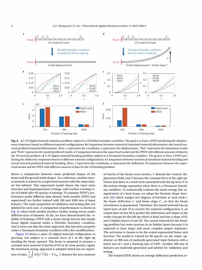
shows a comparison between some predicted shapes of thebeam and the ground truth shapes. As a reference, another neur-al network is trained in a supervised manner with the same data-set but labeled. This supervised model shares the exact samestructure and hyperparameter settings, and reaches a testing er-ror of 0.0036 after 50 epochs of training. To examine PINN's per-formance under different data density, both models (PINN andsupervised) are further trained with 180 and 4500 sets of inputfeatures. The same proportion of validation and testing data arelabeled for each case. A comparison of performance is shown inFig. 2c where both models produce similar testing errors underdifferent sizes of datasets. So far, we have demonstrated the vi-ability of training a PINN with a strain energy loss for this simplelinear digital material under a Dirichlet boundary condition.And it turns out that the same approach also functions properlyunder a Neumann boundary condition with a few modifications.

minv

1

2

∫E I

(v ′′)2

dx −F vtip I

Figure 2d shows a same 1D digital material configuration asprevious, but subject to a constant force of 1 at the right tipbending the beam upward. The beam is assumed to possess aconstant area moment of inertia of 0.6 at its cross section. Again,the minimum energy approach is adopted which has an expres-

sion of . denotes the area moment

v

vi v ′i

of inertia of the beam cross section, denotes the vertical dis-placement field, and F denotes the constant force at the right tip.Notice that there is a work term associated with the tip force F inthe system energy expression when there is a Neumann bound-ary condition. To numerically evaluate the strain energy (the in-tegral term) of a bent beam, we adopt the Hermite shape func-tion [32] which assigns two degrees of freedom at each node i:the beam deflection and beam slope , so that the beamsmoothness is guaranteed. Therefore, the neural network has aninput layer of size 10 to receive the material configuration E, anoutput layer of size 20 to predict the deflections and slopes at thenodes (except for the left tip which is fixed and has a slope of 0),and 3 hidden layers of size 30. The neural network for the bend-ing problem has more neurons in its hidden layers because it isexpected to have larger and more complex output responses.The activation is chosen to be the scaled exponential linear unitfunction. The model is trained for 80 epochs on the Adam op-timizer on 900 sets of randomly generated input features with abatch size of 1 and a learning rate of 0.001. Another 200 sets offeatures are randomly generated and labeled for validation andtesting.

The trained PINN shows an average deflection prediction er-

a d

b e

c f

Fixed

Fixed

Fixed

Fixed

1D composite beam 1D composite beam

Nodal displacements? Nodal displacements? Nodal slopes?

F

uEr

ror

Dirichlet boundary condition:extended by 20% at right tip

Neumann boundary condition:bent by a force at right tip

...E1 E2 E3 E10...E1 E2 E3 E10

0.20

0.15

0.10

0.05

0

6

4

2

0

Erro

r

0.04

0.02

0

0 0.5

180

×10−3

900Number of training data

4500 180 900Number of training data

4500

SupervisedPINN

SupervisedPINN

1.0

u

0.20

0.15

0.10

0.05

00 0.5 1.0

u

0.3

0.2

0.1

00 0.5 1.0

Sim1Sim2Sim3

Sim1Sim2Sim3

Pred1Pred2Pred3

Pred1Pred2Pred3

x x x

u

0.3

0.2

0.1

00 0.5 1.0

x

Fig. 2. a A 1D digital material extension problem subject to a Dirichlet boundary condition. The goal is to have a PINN predicting the displace-ment responses based on different material configurations. b Comparison between numerical simulated material deformation and neural net-work predicted material deformation. Here, x represents the coordinate, u represents the displacement, “Sim” represents the simulation resultsand “Pred” represents the model predicted results. c Comparison between the supervised model and the PINN with different amount of data forthe 1D tension problem. d A 1D digital material bending problem subject to a Neumann boundary condition. The goal is to have a PINN pre-dicting the deflection responses based on different material configurations. e Comparison between numerical simulated material bending andneural network predicted material bending. Here, x represents the coordinate, u represents the deflection. f Comparison between the super-vised model and the PINN with different amount of data for the 1D bending problem.

2 Z.Z. Zhang and G.X. Gu / Theoretical & Applied Mechanics Letters 11 (2021) 000-6

−F vtip

ror of 0.0056 for each node based on the testing set. Figure 2eshows a comparison between some predicted shapes of thebeam and the ground truth shapes. A reference supervised neur-al network with the exact same structure and hyperparametersreaches a testing error of 0.0055 after 80 epochs of training. Theperformance of the PINN and the supervised model is also com-pared under different sizes of datasets as discussed for the ten-sion problem (Fig. 2f). Interestingly, the results of this bendingproblem have two major characteristics. First, the supervisedmodel greatly outperforms the PINN under a low data density(180 sets of training features). Second, using any batch size oth-er than 1 would greatly reduce the training performance. It is be-lieved that these phenomenons are caused by the work term

which assigns a much larger gradient on the right tip de-flection than any other model outputs. This unbalanced gradi-ent can introduce instability during the parameter descent pro-cess which will be explored further in future studies.

The above discussions illustrate the energy-based physics-informed models for intuitive 1D digital materials. However,real-world problems can be more complex in the following as-pects: high order tensor operation for 2D or 3D geometries, non-linear strain as a result of large deformation, computational effi-ciency for evaluating and backpropagating the energy loss,which will be addressed below.

ν

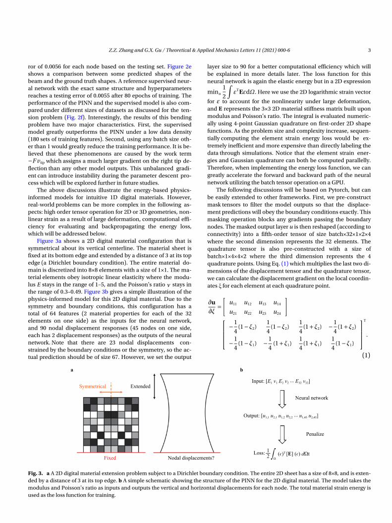
Figure 3a shows a 2D digital material configuration that issymmetrical about its vertical centerline. The material sheet isfixed at its bottom edge and extended by a distance of 3 at its topedge (a Dirichlet boundary condition). The entire material do-main is discretized into 8×8 elements with a size of 1×1. The ma-terial elements obey isotropic linear elasticity where the modu-lus E stays in the range of 1–5, and the Poisson's ratio stays inthe range of 0.3–0.49. Figure 3b gives a simple illustration of thephysics-informed model for this 2D digital material. Due to thesymmetry and boundary conditions, this configuration has atotal of 64 features (2 material properties for each of the 32elements on one side) as the inputs for the neural network,and 90 nodal displacement responses (45 nodes on one side,each has 2 displacement responses) as the outputs of the neuralnetwork. Note that there are 23 nodal displacements con-strained by the boundary conditions or the symmetry, so the ac-tual prediction should be of size 67. However, we set the output

minu

1

2

∫εTEεdΩ

ε

layer size to 90 for a better computational efficiency which willbe explained in more details later. The loss function for thisneural network is again the elastic energy but in a 2D expression

. Here we use the 2D logarithmic strain vector

for to account for the nonlinearity under large deformation,and E represents the 3×3 2D material stiffness matrix built uponmodulus and Poisson's ratio. The integral is evaluated numeric-ally using 4-point Gaussian quadrature on first-order 2D shapefunctions. As the problem size and complexity increase, sequen-tially computing the element strain energy loss would be ex-tremely inefficient and more expensive than directly labeling thedata through simulations. Notice that the element strain ener-gies and Gaussian quadrature can both be computed parallelly.Therefore, when implementing the energy loss function, we cangreatly accelerate the forward and backward path of the neuralnetwork utilizing the batch tensor operation on a GPU.

The following discussions will be based on Pytorch, but canbe easily extended to other frameworks. First, we pre-constructmask tensors to filter the model outputs so that the displace-ment predictions will obey the boundary conditions exactly. Thismasking operation blocks any gradients passing the boundarynodes. The masked output layer u is then reshaped (according toconnectivity) into a fifth-order tensor of size batch×32×1×2×4where the second dimension represents the 32 elements. Thequadrature tensor is also pre-constructed with a size ofbatch×1×4×4×2 where the third dimension represents the 4quadrature points. Using Eq. (1) which multiplies the last two di-mensions of the displacement tensor and the quadrature tensor,we can calculate the displacement gradient on the local coordin-ates ξ for each element at each quadrature point.

∂u

∂ξ=

[u11

u21

u12

u22

u13

u23

u14

u24

] −1

4(1−ξ2)

−1

4(1−ξ1)

1

4(1−ξ2)

−1

4(1+ξ1)

1

4(1+ξ2)

1

4(1+ξ1)

−1

4(1+ξ2)

1

4(1−ξ1)

T

.

(1)

a b

Symmetrical Extended

Fixed Nodal displacements?

Penalize

Neural network

Input: [E1 v1 E2 v2 ... E32 v32]

Output: [u1,1 u2,1 u1,2 u2,2 ... u1,45 u2,45]

Loss: (ϵ)T [E] (ϵ) dΩt∫2 Ω

1

Fig. 3. a A 2D digital material extension problem subject to a Dirichlet boundary condition. The entire 2D sheet has a size of 8×8, and is exten-ded by a distance of 3 at its top edge. b A simple schematic showing the structure of the PINN for the 2D digital material. The model takes themodulus and Poisson's ratio as inputs and outputs the vertical and horizontal displacements for each node. The total material strain energy isused as the loss function for training.

Z.Z. Zhang and G.X. Gu / Theoretical & Applied Mechanics Letters 11 (2021) 000-6 3

∂u/∂x

x

∂u/∂x + I

U2 ε

C

Next, the global displacement gradient (it has a shapeof batch×32×4×2×2) can be obtained by multiplying the localgradient tensor with the mapping tensor from ξ to which is afixed quantity and can be pre-constructed before training. Thedeformation gradient F equals to , where I is a 2×2identity matrix. The Green's deformation tensor C can then becalculated as FTF which further equals to the square of the rightstretch tensor . And the nonlinear logarithmic strain can beobtained by taking the square root and natural log on the eigen-space of (take operations on the eigenvalues of C, then recon-struct the tensor). The strain tensor is then reshaped into a sizeof batch×32×4×3.

νE/(1−ν2) Eν/(1−ν2) E/[2(1+ν)]

ε

For the material stiffness matrix, the input features are aug-mented so that instead of passing E and into the model, wepass , , and for each materialelement (the neural network has an input layer of size 96 in-stead of 64). Thereafter, E (size of batch×32×4×3×3) can be eas-ily constructed by gathering the corresponding input features oneach of its rows without an element-wise value assignment. Thestrain energy of each element at each quadrature point can nowbe parallelly computed on GPU through tensor productsbetween reconstructed and E. The last step is to sum over thesecond (size of 32) and third (size of 4) dimensions of the energytensor to obtain the total strain energy as the prediction loss.

Every step discussed above is a pure tensor operation that isparallelable on a GPU and differentiable. However, the deforma-tion gradient F step may require extra care. Due to the neuralnetwork's ignorance of the physical world, the model is theoret-ically allowed to predict any displacement responses withoutconstraints at the early stages of training. This can produce phys-ically nonexistent F which has a negative determinant. Althoughthe model training can still proceed for such erroneous F, thegradient update for the neural network parameters are likelypointing towards a wrong direction and thus negatively affectthe convergence rate and stability. To overcome this issue, onemethod is to initialize the neural network so that the initialguesses of nodal displacement responses have small mag-nitudes compared to the size of an element (1×1), and the mod-

−min(0, J )el parameters never enter the problematic region. Anothermethod we adopted is adding this extra term to theloss function where J (Jacobian) is the determinant of F. Thisterm has no effect on training when J is positive, but it penalizesand forces the neural network to produce more positive J valueswhenever it predicts an erroneous F.

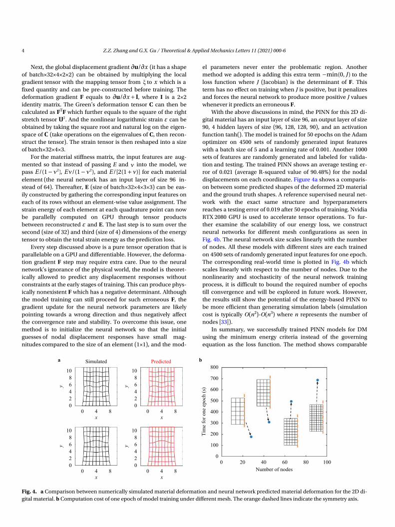
With the above discussions in mind, the PINN for this 2D di-gital material has an input layer of size 96, an output layer of size90, 4 hidden layers of size (96, 128, 128, 90), and an activationfunction tanh(). The model is trained for 50 epochs on the Adamoptimizer on 4500 sets of randomly generated input featureswith a batch size of 5 and a learning rate of 0.001. Another 1000sets of features are randomly generated and labeled for valida-tion and testing. The trained PINN shows an average testing er-ror of 0.021 (average R-squared value of 90.48%) for the nodaldisplacements on each coordinate. Figure 4a shows a comparis-on between some predicted shapes of the deformed 2D materialand the ground truth shapes. A reference supervised neural net-work with the exact same structure and hyperparametersreaches a testing error of 0.019 after 50 epochs of training. NvidiaRTX 2080 GPU is used to accelerate tensor operations. To fur-ther examine the scalability of our energy loss, we constructneural networks for different mesh configurations as seen inFig. 4b. The neural network size scales linearly with the numberof nodes. All these models with different sizes are each trainedon 4500 sets of randomly generated input features for one epoch.The corresponding real-world time is plotted in Fig. 4b whichscales linearly with respect to the number of nodes. Due to thenonlinearity and stochasticity of the neural network trainingprocess, it is difficult to bound the required number of epochstill convergence and will be explored in future work. However,the results still show the potential of the energy-based PINN tobe more efficient than generating simulation labels (simulationcost is typically O(n2)-O(n3) where n represents the number ofnodes [33]).

In summary, we successfully trained PINN models for DMusing the minimum energy criteria instead of the governingequation as the loss function. The method shows comparable

a bSimulated Predicted

y

x

Tim

e fo

r one

epoch

(s)

10

8

6

4

2

00 4 8

y

x

10

8

6

4

2

00 4 8

y

x

10

8

6

4

2

00 4 8

y

x

10

8

6

4

2

00 4 8

800

700

600

500

400

300

200

100

00 20 40 60

Number of nodes

80 100

Fig. 4. a Comparison between numerically simulated material deformation and neural network predicted material deformation for the 2D di-gital material. b Computation cost of one epoch of model training under different mesh. The orange dashed lines indicate the symmetry axis.

4 Z.Z. Zhang and G.X. Gu / Theoretical & Applied Mechanics Letters 11 (2021) 000-6

accuracy to the supervised models on the 1D tension, 1D bend-ing, and 2D tension problems discussed in this paper. Resultsshow that our proposed PINN can properly approximate the log-arithmic strain and fix any erroneous deformation gradient byadding a hinge loss for the Jacobian. Moreover, the loss evalu-ation step can be parallelized over the elements and quadraturepoints on a GPU through proper tensor rearrangements on in-put features and outputs responses. The single epoch computa-tion cost of the optimized algorithm scales linearly with respectto the number of nodes (or elements) in a DM mesh. This workshows the possibility of training PINNs for digital materials ac-curately and efficiently, allowing direct ML exploration of next-generation composite design without the necessity of expensivemulti-physics simulations.

Acknowledgement

The authors acknowledge support from the Extreme Scienceand Engineering Discovery Environment (XSEDE) at the Pitts-burgh Supercomputing Center (PSC) by National ScienceFoundation (Grant ACI-1548562). Additionally, the authors ac-knowledge support from the Chau Hoi Shuen Foundation Wo-men in Science Program and an NVIDIA GPU Seed Grant.

References

I. Gibson, D.W. Rosen, B. Stucker, Additive manufacturingTechnologies, Springer, 2014.

[1]

M. Vaezi, S. Chianrabutra, B. Mellor, et al., Multiple materialadditive manufacturing–Part 1: A review: this review paper cov-ers a decade of research on multiple material additive manu-facturing technologies which can produce complex geometryparts with different materials, Virtual and Physical Prototyping8 (2013) 19–50.

[2]

G.X. Gu, M. Takaffoli, M.J. Buehler, Hierarchically enhancedimpact resistance of bioinspired composites, Advanced Materi-als 29 (2017) 1700060.

[3]

Z. Vangelatos, Z. Zhang, G.X. Gu, et al., Tailoring the dynamicactuation of 3D-printed mechanical metamaterials through in-herent and extrinsic instabilities, Advanced Engineering Mater-ials (2020) 1901586.

[4]

P. Tran, T.D. Ngo, A. Ghazlan, et al., Bimaterial 3D printing andnumerical analysis of bio-inspired composite structures underin-plane and transverse loadings, Composites Part B: Engineer-ing 108 (2017) 210–223.

[5]

J.J. Martin, B.E. Fiore, R.M. Erb, Designing bioinspired compos-ite reinforcement architectures via 3D magnetic printing,Nature Communications 6 (2015) 1–7.

[6]

C.-T. Chen, G.X. Gu, Machine learning for composite materials,MRS Communications 9 (2019) 556–566.

[7]

J.C. Breger, C.K. Yoon, Rui Xiao, et al., Self-folding thermo-magnetically responsive soft microgrippers, ACS Applied Ma-terials & Interfaces 7 (2015) 3398–3405.

[8]

Q. Ge, A.H. Sakhaei, H. Lee, et al., Multimaterial 4D printingwith tailorable shape memory polymers, Scientific Reports 6(2016) 31110.

[9]

R. MacCurdy, R. Katzschmann, Y. Kim, et al., Printable hydraul-ics: A method for fabricating robots by 3D co-printing solidsand liquids, in 2016 IEEE International Conference on Roboticsand Automation (ICRA), (2016) 3878-3885.

[10]

Z. Zhang, K.G. Demir, G.X. Gu, Developments in 4D-printing: areview on current smart materials, technologies, and applica-tions, International Journal of Smart and Nano Materials 10(2019) 205–224.

[11]

Y. Mao, K. Yu, M.S. Isakov, et al., Sequential self-folding struc-tures by 3D printed digital shape memory polymers, ScientificReports 5 (2015) 13616.

[12]

F. Momeni, X. Liu, J. Ni, A review of 4D printing, Materials &Design 122 (2017) 42–79.

[13]

C.T. Chen, G.X. Gu, Generative deep neural networks for in-verse materials design using backpropagation and active learn-ing, Advanced Science (2020) 1902607.

[14]

P.Z. Hanakata, E.D. Cubuk, D.K. Campbell, et al., Acceleratedsearch and design of stretchable graphene kirigami using ma-chine learning,, Physical Review Letters 121 (2018) 255304.

[15]

Z. Zhang, G.X. Gu, Finite-element-based deep-learning modelfor deformation behavior of digital materials, Advanced Theoryand Simulations (2020) 2000031.

[16]

A. Paul, P. Acar, W.-K. Liao, et al., Microstructure optimizationwith constrained design objectives using machine learning-based feedback-aware data-generation, Computational Materi-als Science 160 (2019) 334–351.

[17]

N. Zobeiry, J. Reiner, R. Vaziri, Theory-guided machine learn-ing for damage characterization of composites, CompositeStructures (2020) 112407.

[18]

W. Yan, L. Deng, F. Zhang, et al., Probabilistic machine learn-ing approach to bridge fatigue failure analysis due to vehicularoverloading, Engineering Structures 193 (2019) 91–99.

[19]

Z. Jin, Z. Zhang, G.X. Gu, Autonomous in-situ correction offused deposition modeling printers using computer vision anddeep learning, Manufacturing Letters 22 (2019) 11–15.

[20]

H. Wei, S. Zhao, Q. Rong, et al., Predicting the effective thermalconductivities of composite materials and porous media by ma-chine learning methods, International Journal of Heat andMass Transfer 127 (2018) 908–916.

[21]

B. Zheng, G.X. Gu, Machine learning-based detection ofgraphene defects with atomic precision, Nano-Micro Letters 12(2020) 1–13.

[22]

M. Raissi, P. Perdikaris, G.E. Karniadakis, Physics-informedneural networks: A deep learning framework for solving for-ward and inverse problems involving nonlinear partial differen-tial equations, Journal of Computational Physics 378 (2019)686–707.

[23]

R. Sharma, A.B. Farimani, J. Gomes, et al., Weakly-superviseddeep learning of heat transport via physics informed loss,(2018) arXiv: 1807.11374.

[24]

M. Raissi, A. Yazdani, G.E. Karniadakis, Hidden fluid mechan-ics: Learning velocity and pressure fields from flow visualiza-tions, Science 367 (2020) 1026–1030.

[25]

J.-L. Wu, H. Xiao, E. Paterson, Physics-informed machine learn-ing approach for augmenting turbulence models: A compre-hensive framework, Physical Review Fluids 3 (2018) 074602.

[26]

Y. Yang, P. Perdikaris, Adversarial uncertainty quantification inphysics-informed neural networks, Journal of ComputationalPhysics 394 (2019) 136–152.

[27]

G. Pang, L. Lu, G.E. Karniadakis, fPINNs: Fractional physics-in-formed neural networks, SIAM Journal on Scientific Comput-ing 41 (2019) A2603–A2626.

[28]

Y. Heider, K. Wang, W. Sun, SO(3)-invariance of informed-graph-based deep neural network for anisotropic elastoplastic

[29]

Z.Z. Zhang and G.X. Gu / Theoretical & Applied Mechanics Letters 11 (2021) 000-6 5

materials, Computer Methods in Applied Mechanics and En-

gineering 363 (2020) 112875.

L. Yang, X. Meng, G.E. Karniadakis, B-pinns: Bayesian physics-

informed neural networks for forward and inverse pde prob-

lems with noisy data, arXiv preprint (2020) arXiv: 2003.06097.

[30]

C.-T. Chen, G.X. Gu, Learning hidden elasticity with deep neur-[31]

al networks, arXiv preprint (2020) arXiv: 2010.13534.

W. Weaver Jr, S.P. Timoshenko, D.H. Young, Vibration Prob-

lems in Engineering, John Wiley & Sons, (1990).

[32]

T.I. Zohdi, A Finite Element Primer for Beginners, Springer,

(2018).

[33]

6 Z.Z. Zhang and G.X. Gu / Theoretical & Applied Mechanics Letters 11 (2021) 000-6